Post Syndicated from Navnit Shukla original https://aws.amazon.com/blogs/big-data/accelerate-queries-on-apache-iceberg-tables-through-aws-glue-auto-compaction/
Data lakes were originally designed to store large volumes of raw, unstructured, or semi-structured data at a low cost, primarily serving big data and analytics use cases. Over time, as organizations began to explore broader applications, data lakes have become essential for various data-driven processes beyond just reporting and analytics. Today, they play a critical role in syncing with customer applications, enabling the ability to manage concurrent data operations while maintaining the integrity and consistency of information. This shift includes not only storing batch data but also ingesting and processing near real-time data streams, allowing businesses to merge historical insights with live data to power more responsive and adaptive decision-making. However, this new data lake architecture brings challenges around managing transactional support and handling the influx of small files generated by real-time data streams. Traditionally, customers addressed these challenges by performing complex extract, transform, and load (ETL) processes, which often led to data duplication and increased complexity in data pipelines. Additionally, to cope with the proliferation of small files, organizations had to develop custom mechanisms to compact and merge these files, leading to the creation and maintenance of bespoke solutions that were difficult to scale and manage. As data lakes increasingly handle sensitive business data and transactional workloads, maintaining strong data quality, governance, and compliance becomes vital to maintaining trust and regulatory alignment.
To simplify these challenges, organizations have adopted open table formats (OTFs) like Apache Iceberg, which provide built-in transactional capabilities and mechanisms for compaction. OTFs, such as Iceberg, address key limitations in traditional data lakes by offering features like ACID transactions, which maintain data consistency across concurrent operations, and compaction, which helps manage the issue of small files by merging them efficiently. By using features like Iceberg’s compaction, OTFs streamline maintenance, making it straightforward to manage object and metadata versioning at scale. However, although OTFs reduce the complexity of maintaining efficient tables, they still require some regular maintenance to make sure tables remain in an optimal state.
In this post, we explore new features of the AWS Glue Data Catalog, which now supports improved automatic compaction of Iceberg tables for streaming data, making it straightforward for you to keep your transactional data lakes consistently performant. Enabling automatic compaction on Iceberg tables reduces metadata overhead on your Iceberg tables and improves query performance. Many customers have streaming data continuously ingested in Iceberg tables, resulting in a large number of delete files that track changes in data files. With this new feature, as you enable the Data Catalog optimizer. It constantly monitors table partitions and runs the compaction process for both data and delta or delete files, and it regularly commits partial progress. The Data Catalog also now supports heavily nested complex data and supports schema evolution as you reorder or rename columns.
Automatic compaction with AWS Glue
Automatic compaction in the Data Catalog makes sure your Iceberg tables are always in optimal condition. The data compaction optimizer continuously monitors table partitions and invokes the compaction process when specific thresholds for the number of files and file sizes are met. For example, based on the Iceberg table configuration of the target file size, the compaction process will start and continue if the table or any of the partitions within the table have more than the default configuration (for example 100 files), each smaller than 75% of the target file size.
Iceberg supports two table modes: Merge-on-Read (MoR) and Copy-on-Write (CoW). These table modes provide different approaches for handling data updates and play a critical role in how data lakes manage changes and maintain performance:
- Data compaction on Iceberg CoW – With CoW, any updates or deletes are directly applied to the table files. This means the entire dataset is rewritten when changes are made. Although this provides immediate consistency and simplifies reads (because readers only access the latest snapshot of the data), it can become costly and slow for write-heavy workloads due to the need for frequent rewrites. Announced during AWS re:Invent 2023, this feature focuses on optimizing data storage for Iceberg tables using the CoW mechanism. Compaction in CoW makes sure updates to the data result in new files being created, which are then compacted to improve query performance.
- Data compaction on Iceberg MoR – Unlike CoW, MoR allows updates to be written separately from the existing dataset, and those changes are only merged when the data is read. This approach is beneficial for write-heavy scenarios because it avoids frequent full table rewrites. However, it can introduce complexity during reads because the system has to merge base and delta files as needed to provide a complete view of the data. MoR compaction, now generally available, allows for efficient handling of streaming data. It makes sure that while data is being continuously ingested, it’s also compacted in a way that optimizes read performance without compromising the ingestion speed.
Whether you are using CoW, MoR, or a hybrid of both, one challenge remains consistent: maintenance around the growing number of small files generated by each transaction. AWS Glue automatic compaction addresses this by making sure your Iceberg tables remain efficient and performant across both table modes.
This post provides a detailed comparison of query performance between auto compacted and non-compacted Iceberg tables. By analyzing key metrics such as query latency and storage efficiency, we demonstrate how the automatic compaction feature optimizes data lakes for better performance and cost savings. This comparison will help guide you in making informed decisions on enhancing your data lake environments.
Solution overview
This blog post explores the performance benefits of the newly launched feature in AWS Glue that supports automatic compaction of Iceberg tables with MoR capabilities. We run two versions of the same architecture: one where the tables are auto compacted, and another without compaction. By comparing both scenarios, this post demonstrates the efficiency, query performance, and cost benefits of auto compacted tables vs. non-compacted tables in a simulated Internet of Things (IoT) data pipeline.
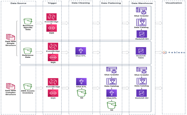
The following diagram illustrates the solution architecture.

The solution consists of the following components:
- Amazon Elastic Compute Cloud (Amazon EC2) simulates continuous IoT data streams, sending them to Amazon MSK for processing
- Amazon Managed Streaming for Apache Kafka (Amazon MSK) ingests and streams data from the IoT simulator for real-time processing
- Amazon EMR Serverless processes streaming data from Amazon MSK without managing clusters, writing results to the Amazon S3 data lake
- Amazon Simple Storage Service (Amazon S3) stores data using Iceberg’s MoR format for efficient querying and analysis
- The Data Catalog manages metadata for the datasets in Amazon S3, enabling organized data discovery and querying through Amazon Athena
- Amazon Athena queries data from the S3 data lake with two table options:
- Non-compacted table – Queries raw data from the Iceberg table
- Compacted table – Queries data optimized by automatic compaction for faster performance.
The data flow consists of the following steps:
- The IoT simulator on Amazon EC2 generates continuous data streams.
- The data is sent to Amazon MSK, which acts as a streaming table.
- EMR Serverless processes streaming data and writes the output to Amazon S3 in Iceberg format.
- The Data Catalog manages the metadata for the datasets.
- Athena is used to query the data, either directly from the non-compacted table or from the compacted table after auto compaction.
In this post, we guide you through setting up an evaluation environment for AWS Glue Iceberg auto compaction performance using the following GitHub repository. The process involves simulating IoT data ingestion, deduplication, and querying performance using Athena.
We simulated IoT data ingestion with over 20 billion events and used MERGE INTO for data deduplication across two time-based partitions, involving heavy partition reads and shuffling. After ingestion, we ran queries in Athena to compare performance between compacted and non-compacted tables using the MoR format. This test aims to have low latency on ingestion but will lead to hundreds of millions of small files.
We use the following table configuration settings:
'write.delete.mode'='merge-on-read'
'write.update.mode'='merge-on-read'
'write.merge.mode'='merge-on-read'
'write.distribution.mode=none'
We use 'write.distribution.mode=none' to lower the latency. However, it will increase the number of Parquet files. For other scenarios, you may want to use hash or range distribution write modes to reduce the file count.
This test makes make append operations because we’re appending new data to the table but we don’t have any delete operations.
The following table shows some metrics of the Athena query performance.
|
Execution Time (sec) |
Performance Improvement (%) |
Data Scanned (GB) |
| Query |
employee (without compaction) |
employeeauto (with compaction) |
– |
employee (without compaction) |
employeeauto (with compaction) |
SELECT count(*) FROM "bigdata"."<tablename>" |
67.5896 |
3.8472 |
94.31% |
0 |
0 |
SELECT team, name, min(age) AS youngest_age
 FROM "bigdata"."<tablename>"
 GROUP BY team, name
ORDER BY youngest_age ASC |
72.0152 |
50.4308 |
29.97% |
33.72 |
32.96 |
SELECT role, team, avg(age) AS average_age
 FROM bigdata."<tablename>"
 GROUP BY role, team
ORDER BY average_age DESC |
74.1430 |
37.7676 |
49.06% |
17.24 |
16.59 |
SELECT name, age, start_date, role, team
FROM bigdata."<tablename>"
WHERE
CAST(start_date as DATE) > CAST('2023-01-02' as DATE) and
age > 40
ORDER BY start_date DESC
limit 100 |
70.3376 |
37.1232 |
47.22% |
105.74 |
110.32 |
Because the previous test didn’t perform any delete operations on the table, we conduct a new test involving hundreds of thousands of such operations. We use the previously auto compacted table (employeeauto) as a base, noting that this table uses MoR for all operations.
We run a query that deletes data from each even second on the table:
DELETE FROM iceberg_catalog.bigdata.employeeauto
WHERE start_date BETWEEN 'start' AND 'end'
AND SECOND(start_date) % 2 = 0;
This query runs with table optimizations enabled, using an Amazon EMR Studio notebook. After running the queries, we roll back the table to its previous state for a performance comparison. Iceberg’s time-traveling capabilities allow us to restore the table. We then disable the table optimizations, rerun the delete query, and follow up with Athena queries to analyze performance differences. The following table summarizes our results.
|
Execution Time (sec) |
Performance Improvement (%) |
Data Scanned (GB) |
| Query |
employee (without compaction) |
employeeauto (with compaction) |
– |
employee (without compaction) |
employeeauto (with compaction) |
SELECT count(*) FROM "bigdata"."<tablename>" |
29.820 |
8.71 |
70.77% |
0 |
0 |
SELECT team, name, min(age) as youngest_age
FROM "bigdata"."<tablename>"
GROUP BY team, name
ORDER BY youngest_age ASC |
58.0600 |
34.1320 |
41.21% |
33.27 |
19.13 |
SELECT role, team, avg(age) AS average_age
FROM bigdata."<tablename>"
GROUP BY role, team
ORDER BY average_age DESC |
59.2100 |
31.8492 |
46.21% |
16.75 |
9.73 |
SELECT name, age, start_date, role, team
FROM bigdata."<tablename>"
WHERE
CAST(start_date as DATE) > CAST('2023-01-02' as DATE) and
age > 40
ORDER BY start_date DESC
limit 100 |
68.4650 |
33.1720 |
51.55% |
112.64 |
61.18 |
We analyze the following key metrics:
- Query runtime – We compared the runtimes between compacted and non-compacted tables using Athena as the query engine and found significant performance improvements with both MoR for ingestion and appends and MoR for delete operations.
- Data scanned evaluation – We compared compacted and non-compacted tables using Athena as the query engine and observed a reduction in data scanned for most queries. This reduction translates directly into cost savings.
Prerequisites
To set up your own evaluation environment and test the feature, you need the following prerequisites:
- A virtual private cloud (VPC) with at least two private subnets. For instructions, see Create a VPC.
- An EC2 instance c5.xlarge using Amazon Linux 2023 running on one of those private subnets where you will launch the data simulator. For the security group, you can use the default for the VPC. For more information, see Get started with Amazon EC2.
- An AWS Identity and Access Management (IAM) user with the correct permissions to create and configure all the required resources.
Set up Amazon S3 storage
Create an S3 bucket with the following structure:
s3bucket/
/jars
/employee.desc
/warehouse
/checkpoint
/checkpointAuto
Download the descriptor file employee.desc from the GitHub repo and place it in the S3 bucket.
Download the application on the releases page
Get the packaged application from the GitHub repo, then upload the JAR file to the jars directory on the S3 bucket. The warehouse will be where the Iceberg data and metadata will live and checkpoint will be used for the Structured Streaming checkpointing mechanism. Because we use two streaming job runs, one for compacted and one for non-compacted data, we also create a checkpointAuto folder.
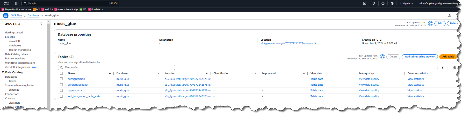
Create a Data Catalog database
Create a database in the Data Catalog (for this post, we name our database bigdata). For instructions, see Getting started with the AWS Glue Data Catalog.
Create an EMR Serverless application
Create an EMR Serverless application with the following settings (for instructions, see Getting started with Amazon EMR Serverless):
- Type: Spark
- Version: 7.1.0
- Architecture: x86_64
- Java Runtime: Java 17
- Metastore Integration: AWS Glue Data Catalog
- Logs: Enable Amazon CloudWatch Logs if desired
Configure the network (VPC, subnets, and default security group) to allow the EMR Serverless application to reach the MSK cluster.
Take note of the application-id to use later for launching the jobs.
Create an MSK cluster
Create an MSK cluster on the Amazon MSK console. For more details, see Get started using Amazon MSK.
You need to use custom create with at least two brokers using 3.5.1, Apache Zookeeper mode version, and instance type kafka.m7g.xlarge. Do not use public access; choose two private subnets to deploy it (one broker per subnet or Availability Zone, for a total of two brokers). For the security group, remember that the EMR cluster and the Amazon EC2 based producer will need to reach the cluster and act accordingly. For security, use PLAINTEXT (in production, you should secure access to the cluster). Choose 200 GB as storage size for each broker and do not enable tiered storage. For network security groups, you can choose the default of the VPC.
For the MSK cluster configuration, use the following settings:
auto.create.topics.enable=true
default.replication.factor=2
min.insync.replicas=2
num.io.threads=8
num.network.threads=5
num.partitions=32
num.replica.fetchers=2
replica.lag.time.max.ms=30000
socket.receive.buffer.bytes=102400
socket.request.max.bytes=104857600
socket.send.buffer.bytes=102400
unclean.leader.election.enable=true
zookeeper.session.timeout.ms=18000
compression.type=zstd
log.retention.hours=2
log.retention.bytes=10073741824
Log in to your EC2 instance. Because it’s running on a private subnet, you can use an instance endpoint to connect. To create one, see Connect to your instances using EC2 Instance Connect Endpoint. After you log in, issue the following commands:
sudo yum install java-17-amazon-corretto-devel
wget https://archive.apache.org/dist/kafka/3.5.1/kafka_2.12-3.5.1.tgz
tar xzvf kafka_2.12-3.5.1.tgz
Create Kafka topics
Create two Kafka topics—remember that you need to change the bootstrap server with the corresponding client information. You can get this data from the Amazon MSK console on the details page for your MSK cluster.

cd kafka_2.12-3.5.1/bin/

./kafka-topics.sh --topic protobuf-demo-topic-pure-auto --bootstrap-server kafkaBoostrapString --create
./kafka-topics.sh --topic protobuf-demo-topic-pure --bootstrap-server kafkaBoostrapString –create
Launch job runs
Issue job runs for the non-compacted and auto compacted tables using the following AWS Command Line Interface (AWS CLI) commands. You can use AWS CloudShell to run the commands.
For the non-compacted table, you need to change the s3bucket value as needed and the application-id. You also need an IAM role (execution-role-arn) with the corresponding permissions to access the S3 bucket and to access and write tables on the Data Catalog.
aws emr-serverless start-job-run --application-id application-identifier --name job-run-name --execution-role-arn arn-of-emrserverless-role --mode 'STREAMING' --job-driver '{
"sparkSubmit": {
"entryPoint": "s3://s3bucket/jars/streaming-iceberg-ingest-1.0-SNAPSHOT.jar",
"entryPointArguments": ["true","s3://s3bucket/warehouse","s3://s3bucket/Employee.desc","s3://s3bucket/checkpoint","kafkaBootstrapString","true"],
"sparkSubmitParameters": "--class com.aws.emr.spark.iot.SparkCustomIcebergIngestMoR --conf spark.executor.cores=16 --conf spark.executor.memory=64g --conf spark.driver.cores=4 --conf spark.driver.memory=16g --conf spark.dynamicAllocation.minExecutors=3 --conf spark.jars=/usr/share/aws/iceberg/lib/iceberg-spark3-runtime.jar --conf spark.dynamicAllocation.maxExecutors=5 --conf spark.sql.catalog.glue_catalog.http-client.apache.max-connections=3000 --conf spark.emr-serverless.executor.disk.type=shuffle_optimized --conf spark.emr-serverless.executor.disk=1000G --files s3://s3bucket/Employee.desc --packages org.apache.spark:spark-sql-kafka-0-10_2.12:3.5.1"
}
}'
For the auto compacted table, you need to change the s3bucket value as needed, the application-id, and the kafkaBootstrapString. You also need an IAM role (execution-role-arn) with the corresponding permissions to access the S3 bucket and to access and write tables on the Data Catalog.
aws emr-serverless start-job-run --application-id application-identifier --name job-run-name --execution-role-arn arn-of-emrserverless-role --mode 'STREAMING' --job-driver '{
"sparkSubmit": {
"entryPoint": "s3://s3bucket/jars/streaming-iceberg-ingest-1.0-SNAPSHOT.jar",
"entryPointArguments": ["true","s3://s3bucket/warehouse","/home/hadoop/Employee.desc","s3://s3bucket/checkpointAuto","kafkaBootstrapString","true"],
"sparkSubmitParameters": "--class com.aws.emr.spark.iot.SparkCustomIcebergIngestMoRAuto --conf spark.executor.cores=16 --conf spark.executor.memory=64g --conf spark.driver.cores=4 --conf spark.driver.memory=16g --conf spark.dynamicAllocation.minExecutors=3 --conf spark.jars=/usr/share/aws/iceberg/lib/iceberg-spark3-runtime.jar --conf spark.dynamicAllocation.maxExecutors=5 --conf spark.sql.catalog.glue_catalog.http-client.apache.max-connections=3000 --conf spark.emr-serverless.executor.disk.type=shuffle_optimized --conf spark.emr-serverless.executor.disk=1000G --files s3://s3bucket/Employee.desc --packages org.apache.spark:spark-sql-kafka-0-10_2.12:3.5.1"
}
}'
Enable auto compaction
Enable auto compaction for the employeeauto table in AWS Glue. For instructions, see Enabling compaction optimizer.
Launch the data simulator
Download the JAR file to the EC2 instance and run the producer:
aws s3 cp s3://s3bucket/jars/streaming-iceberg-ingest-1.0-SNAPSHOT.jar .
Now you can start the protocol buffer producers.
For non-compacted tables, use the following commands:
java -cp streaming-iceberg-ingest-1.0-SNAPSHOT.jar
com.aws.emr.proto.kafka.producer.ProtoProducer kafkaBoostrapString
For auto compacted tables, use the following commands:
java -cp streaming-iceberg-ingest-1.0-SNAPSHOT.jar
com.aws.emr.proto.kafka.producer.ProtoProducerAuto kafkaBoostrapString
Test the solution in EMR Studio
For the delete test, we use an EMR Studio. For setup instructions, see Set up an EMR Studio. Next, you need to create an EMR Serverless interactive application to run the notebook; refer to Run interactive workloads with EMR Serverless through EMR Studio to create a Workspace.
Open the Workspace, select the interactive EMR Serverless application as the compute option, and attach it.

Download the Jupyter notebook, upload it to your environment, and run the cells using a PySpark kernel to run the test.
Clean up
This evaluation is for high-throughput scenarios and can lead to significant costs. Complete the following steps to clean up your resources:
- Stop the Kafka producer EC2 instance.
- Cancel the EMR job runs and delete the EMR Serverless application.
- Delete the MSK cluster.
- Delete the tables and database from the Data Catalog.
- Delete the S3 bucket.
Conclusion
The Data Catalog has improved automatic compaction of Iceberg tables for streaming data, making it straightforward for you to keep your transactional data lakes always performant. Enabling automatic compaction on Iceberg tables reduces metadata overhead on your Iceberg tables and improves query performance.
Many customers have streaming data that is continuously ingested in Iceberg tables, resulting in a large set of delete files that track changes in data files. With this new feature, when you enable the Data Catalog optimizer, it constantly monitors table partitions and runs the compaction process for both data and delta or delete files and regularly commits the partial progress. The Data Catalog also has expanded support for heavily nested complex data and supports schema evolution as you reorder or rename columns.
In this post, we assessed the ingestion and query performance of simulated IoT data using AWS Glue Iceberg with auto compaction enabled. Our setup processed over 20 billion events, managing duplicates and late-arriving events, and employed a MoR approach for both ingestion/appends and deletions to evaluate the performance improvement and efficiency.
Overall, AWS Glue Iceberg with auto compaction proves to be a robust solution for managing high-throughput IoT data streams. These enhancements lead to faster data processing, shorter query times, and more efficient resource utilization, all of which are essential for any large-scale data ingestion and analytics pipeline.
For detailed setup instructions, see the GitHub repo.
About the Authors
 Navnit Shukla serves as an AWS Specialist Solutions Architect with a focus on Analytics. He possesses a strong enthusiasm for assisting clients in discovering valuable insights from their data. Through his expertise, he constructs innovative solutions that empower businesses to arrive at informed, data-driven choices. Notably, Navnit Shukla is the accomplished author of the book titled Data Wrangling on AWS. He can be reached through LinkedIn.
 Angel Conde Manjon is a Sr. PSA Specialist on Data & AI, based in Madrid, and focuses on EMEA South and Israel. He has previously worked on research related to data analytics and artificial intelligence in diverse European research projects. In his current role, Angel helps partners develop businesses centered on data and AI.
Amit Singh currently serves as a Senior Solutions Architect at AWS, specializing in analytics and IoT technologies. With extensive expertise in designing and implementing large-scale distributed systems, Amit is passionate about empowering clients to drive innovation and achieve business transformation through AWS solutions.
Sandeep Adwankar is a Senior Technical Product Manager at AWS. Based in the California Bay Area, he works with customers around the globe to translate business and technical requirements into products that enable customers to improve how they manage, secure, and access data.


 Michael Davies is a Data Engineer at OUA. He has extensive experience within the education industry, with a particular focus on building robust and efficient data architecture and pipelines.
 Emma Arrigo is a Solutions Architect at AWS, focusing on education customers across Australia. She specializes in leveraging cloud technology and machine learning to address complex business challenges in the education sector. Emma’s passion for data extends beyond her professional life, as evidenced by her dog named Data.


 Sean Zou is a Cloud Operations leader with MuleSoft at Salesforce. Sean has been involved in many aspects of MuleSoft’s Cloud Operations, and helped drive MuleSoft’s cloud infrastructure to scale more than tenfold in 7 years. He built the Oversight Engineering function at MuleSoft from scratch.
 Terry Quan focuses on FinOps issues. He works on MuleSoft Engineering on cloud computing budgets and forecasting, cost reduction efforts, costs-to-serve, and coordinates with Salesforce Finance. Terry is a FinOps Practitioner and Professional Certified.
 Audrey Yuan is a Software Engineer with MuleSoft at Salesforce. Audrey works on data lakehouse solutions to help drive cloud maturity across the six pillars of the Well-Architected Framework.
 Rueben Jimenez is a Senior Solutions Architect at AWS, designing and implementing complex data analytics, AI/ML, and cloud infrastructure solutions.
 Avijit Goswami is a Principal Solutions Architect at AWS specialized in data and analytics. He supports AWS strategic customers in building high-performing, secure, and scalable data lake solutions on AWS using AWS managed services and open source solutions. Outside of his work, Avijit likes to travel, hike, watch sports, and listen to music.


 Navnit Shukla serves as an AWS Specialist Solutions Architect with a focus on Analytics. He possesses a strong enthusiasm for assisting clients in discovering valuable insights from their data. Through his expertise, he constructs innovative solutions that empower businesses to arrive at informed, data-driven choices. Notably, Navnit Shukla is the accomplished author of the book titled Data Wrangling on AWS. He can be reached through
  Angel Conde Manjon is a Sr. PSA Specialist on Data & AI, based in Madrid, and focuses on EMEA South and Israel. He has previously worked on research related to data analytics and artificial intelligence in diverse European research projects. In his current role, Angel helps partners develop businesses centered on data and AI.
 Amit Singh currently serves as a Senior Solutions Architect at AWS, specializing in analytics and IoT technologies. With extensive expertise in designing and implementing large-scale distributed systems, Amit is passionate about empowering clients to drive innovation and achieve business transformation through AWS solutions.
 Sandeep Adwankar is a Senior Technical Product Manager at AWS. Based in the California Bay Area, he works with customers around the globe to translate business and technical requirements into products that enable customers to improve how they manage, secure, and access data.


 Xu Feng is a Senior Industry Solution Architect at AWS, responsible for designing, building, and promoting industry solutions for the Media & Entertainment and Advertising sectors, such as intelligent customer service and business intelligence. With 20 years of software industry experience, currently focused on researching and implementing generative AI and AI-powered data solutions.
 Xu Da is a Amazon Web Services (AWS) Partner Solutions Architect based out of Shanghai, China. He has more than 25 years of experience in IT industry, software development and solution architecture. He is passionate about collaborative learning, knowledge sharing, and guiding community in their cloud technologies journey.


 Raj Ramasubbu is a Sr. Analytics Specialist Solutions Architect focused on big data and analytics and AI/ML with Amazon Web Services. He helps customers architect and build highly scalable, performant, and secure cloud-based solutions on AWS. Raj provided technical expertise and leadership in building data engineering, big data analytics, business intelligence, and data science solutions for over 20 years prior to joining AWS. He helped customers in various industry verticals like healthcare, medical devices, life science, retail, asset management, car insurance, residential REIT, agriculture, title insurance, supply chain, document management, and real estate.
 Srividya Parthasarathy is a Senior Big Data Architect on the AWS Lake Formation team. She works with product team and customer to build robust features and solutions for their analytical data platform. She enjoys building data mesh solutions and sharing them with the community.
 Pratik Das is a Senior Product Manager with AWS Lake Formation. He is passionate about all things data and works with customers to understand their requirements and build delightful experiences. He has a background in building data-driven solutions and machine learning systems in production.


 Leo Ramsamy is a Platform Architect specializing in data and analytics for ANZ’s Institutional division. He focuses on modern data practices, including Data Mesh architecture, data governance, quality management, and observability. His work aligns data strategies with business goals, improving accessibility and enabling better decision-making across ANZ.
 Srinivasan Kuppusamy is a Senior Cloud Architect – Data at AWS ProServe, where he helps customers solve their business problems using the power of AWS Cloud technology. His areas of interests are data and analytics, data governance, and AI/ML.
 Rada Stanic is a Chief Technologist at Amazon Web Services, where she helps ANZ customers across different segments solve their business problems using AWS Cloud technologies. Her special areas of interest are data analytics, machine learning/AI, and application modernization.


 AWS customers make use of
 Table buckets are the third type of S3 bucket, taking their place alongside the existing


 Diego Garcia Garcia is a Specialist SA Manager for Analytics at AWS. His expertise spans across Amazon’s analytics services, with a particular focus on real-time data processing and advanced analytics architectures. Diego leads a team of specialist solutions architects across EMEA, collaborating closely with customers spanning across multiple industries and geographies to design and implement solutions to their data analytics challenges.
 Francisco Morillo is a Streaming Solutions Architect at AWS. Francisco works with AWS customers, helping them design real-time analytics architectures using AWS services, supporting Amazon Managed Streaming for Apache Kafka (Amazon MSK) and Amazon Managed Service for Apache Flink.
 Phaneendra Vuliyaragoli is a Product Management Lead for Amazon Data Firehose at AWS. In this role, Phaneendra leads the product and go-to-market strategy for Amazon Data Firehose.


