Post Syndicated from Uday Narayanan original https://aws.amazon.com/blogs/architecture/field-notes-how-to-enable-cross-account-access-for-amazon-kinesis-data-streams-using-kinesis-client-library-2-x/

Businesses today are dealing with vast amounts of real-time data they need to process and analyze to generate insights. Real-time delivery of data and insights enable businesses to quickly make decisions in response to sensor data from devices, clickstream events, user engagement, and infrastructure events, among many others.

Amazon Kinesis Data Streams offers a managed service that lets you focus on building and scaling your streaming applications for near real-time data processing, rather than managing infrastructure. Customers can write Kinesis Data Streams consumer applications to read data from Kinesis Data Streams and process them per their requirements.

Often, the Kinesis Data Streams and consumer applications reside in the same AWS account. However, there are scenarios where customers follow a multi-account approach resulting in Kinesis Data Streams and consumer applications operating in different accounts. Some reasons for using the multi-account approach are to:

• Allocate AWS accounts to different teams, projects, or products for rapid innovation, while still maintaining unique security requirements.
• Simplify AWS billing by mapping AWS costs specific to product or service line.
• Isolate accounts for specific security or compliance requirements.
• Scale resources and mitigate hard AWS service limits constrained to a single account.

The following options allow you to access Kinesis Data Streams across accounts.

• Amazon Kinesis Client Library (KCL) for Java or using the MultiLang Daemon for KCL.
• Amazon Kinesis Data Analytics for Apache Flink – Cross-account access is supported for both Java and Python. For detailed implementation guidance, review the AWS documentation page for Kinesis Data Analytics.
• AWS Glue Streaming – The documentation for AWS Glue describes how to configure AWS Glue streaming ETL jobs to access cross-account Kinesis Data Streams.
• AWS Lambda – Lambda currently does not support cross-account invocations from Amazon Kinesis, but a workaround can be used.

In this blog post, we will walk you through the steps to configure KCL for Java and Python for cross-account access to Kinesis Data Streams.

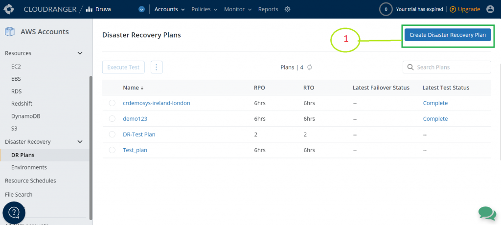
Overview of solution

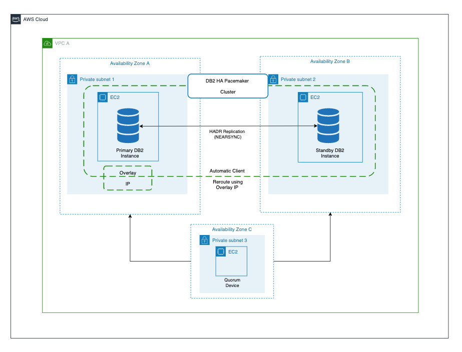
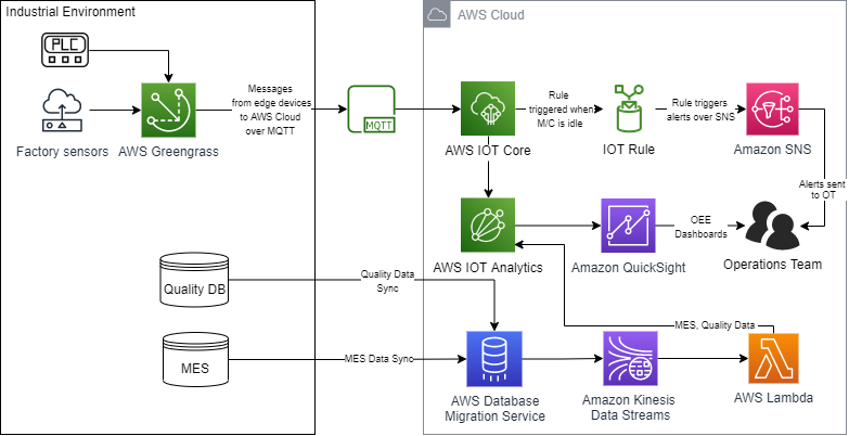
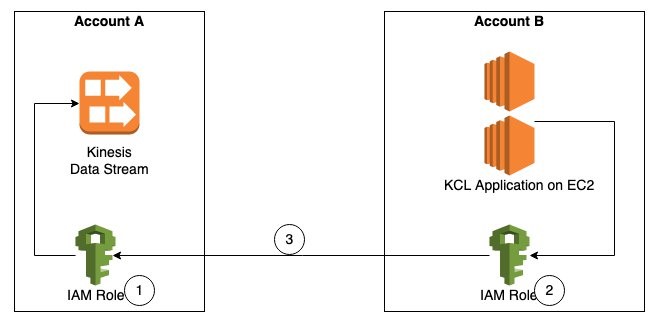
As shown in Figure 1, Account A has the Kinesis data stream and Account B has the KCL instances consuming from the Kinesis data stream in Account A. For the purposes of this blog post the KCL code is running on Amazon Elastic Compute Cloud (Amazon EC2).

The steps to access a Kinesis data stream in one account from a KCL application in another account are:

Step 1 – Create AWS Identity and Access Management (IAM) role in Account A to access the Kinesis data stream with trust relationship with Account B.

Step 2 – Create IAM role in Account B to assume the role in Account A. This role is attached to the EC2 fleet running the KCL application.

Step 3 – Update the KCL application code to assume the role in Account A to read Kinesis data stream in Account A.

Prerequisites

• KCL for Java version 2.3.4 or later.
• AWS Security Token Service (AWS STS) SDK.
• Create a Kinesis data stream named StockTradeStream in Account A and a producer to load data into the stream. If you do not have a producer, you can use the Amazon Kinesis Data Generator to send test data into your Kinesis data stream.

Walkthrough

Step 1 – Create IAM policies and IAM role in Account A

First, we will create an IAM role in Account A, with permissions to access the Kinesis data stream created in the same account. We will also add Account B as a trusted entity to this role.

1. Create IAM policy kds-stock-trade-stream-policy to access Kinesis data stream in Account A using the following policy definition. This policy restricts access to specific Kinesis data stream.

{
    "Version": "2012-10-17",
    "Statement": [
        {
            "Sid": "Stmt123",
            "Effect": "Allow",
            "Action": [
                "kinesis:DescribeStream",
                "kinesis:GetShardIterator",
                "kinesis:GetRecords",
                "kinesis:ListShards",
                "kinesis:DescribeStreamSummary",
                "kinesis:RegisterStreamConsumer"
            ],
            "Resource": [
                "arn:aws:kinesis:us-east-1:Account-A-AccountNumber:stream/StockTradeStream"
            ]
        },
        {
            "Sid": "Stmt234",
            "Effect": "Allow",
            "Action": [
                "kinesis:SubscribeToShard",
                "kinesis:DescribeStreamConsumer"
            ],
            "Resource": [
                "arn:aws:kinesis:us-east-1:Account-A-AccountNumber:stream/StockTradeStream/*"
            ]
        }
    ]
}

Note: The above policy assumes the name of the Kinesis data stream is StockTradeStream.

2. Create IAM role kds-stock-trade-stream-role in Account A.

aws iam create-role --role-name kds-stock-trade-stream-role --assume-role-policy-document "{\"Version\":\"2012-10-17\",\"Statement\":[{\"Effect\":\"Allow\",\"Principal\":{\"AWS\":[\"arn:aws:iam::Account-B-AccountNumber:root\"]},\"Action\":[\"sts:AssumeRole\"]}]}"

3. Attach the kds-stock-trade-stream-policy IAM policy to kds-stock-trade-stream-role role.

aws iam attach-role-policy --policy-arn arn:aws:iam::Account-A-AccountNumber:policy/kds-stock-trade-stream-policy --role-name kds-stock-trade-stream-role

In the above steps, you will have to replace Account-A-AccountNumber with the AWS account number of the account that has the Kinesis data stream and Account-B-AccountNumber will need to be replaced with the AWS account number of the account that has the KCL application

Step 2 – Create IAM policies and IAM role in Account B

We will now create an IAM role in account B to assume the role created in Account A in Step 1. This role will also grant the KCL application access to Amazon DynamoDB and Amazon CloudWatch in Account B. For every KCL application, a DynamoDB table is used to keep track of the shards in a Kinesis data stream that are being leased and processed by the workers of the KCL consumer application. The name of the DynamoDB table is the same as the KCL application name. Similarly, the KCL application needs access to emit metrics to CloudWatch. Because the KCL application is running in Account B, we want to maintain the DynamoDB table and the CloudWatch metrics in the same account as the application code. For this blog post, our KCL application name is StockTradesProcessor.

1. Create IAM policy kcl-stock-trader-app-policy, with permissions access to DynamoDB and CloudWatch in Account B, and to assume the kds-stock-trade-stream-role role created in Account A.

{
    "Version": "2012-10-17",
    "Statement": [
        {
            "Sid": "AssumeRoleInSourceAccount",
            "Effect": "Allow",
            "Action": "sts:AssumeRole",
            "Resource": "arn:aws:iam::Account-A-AccountNumber:role/kds-stock-trade-stream-role"
        },
        {
            "Sid": "Stmt456",
            "Effect": "Allow",
            "Action": [
                "dynamodb:CreateTable",
                "dynamodb:DescribeTable",
                "dynamodb:Scan",
                "dynamodb:PutItem",
                "dynamodb:GetItem",
                "dynamodb:UpdateItem",
                "dynamodb:DeleteItem"
            ],
            "Resource": [
                "arn:aws:dynamodb:us-east-1:Account-B-AccountNumber:table/StockTradesProcessor"
            ]
        },
        {
            "Sid": "Stmt789",
            "Effect": "Allow",
            "Action": [
                "cloudwatch:PutMetricData"
            ],
            "Resource": [
                "*"
            ]
        }
    ]
}

The above policy gives access to a DynamoDB table StockTradesProcessor. If you change you KCL application name, make sure you change the above policy to reflect the corresponding DynamoDB table name.

2. Create role kcl-stock-trader-app-role in Account B to assume role in Account A.

aws iam create-role --role-name kcl-stock-trader-app-role --assume-role-policy-document "{\"Version\":\"2012-10-17\",\"Statement\":[{\"Effect\":\"Allow\",\"Principal\":{\"Service\":[\"ec2.amazonaws.com\"]},\"Action\":[\"sts:AssumeRole\"]}]}"

3. Attach the policy kcl-stock-trader-app-policy to the kcl-stock-trader-app-role.

aws iam attach-role-policy --policy-arn arn:aws:iam::Account-B-AccountNumber:policy/kcl-stock-trader-app-policy --role-name kcl-stock-trader-app-role

4. Create an instance profile with a name as kcl-stock-trader-app-role.

aws iam create-instance-profile --instance-profile-name kcl-stock-trader-app-role

5. Attach the kcl-stock-trader-app-role role to the instance profile.

aws iam add-role-to-instance-profile --instance-profile-name kcl-stock-trader-app-role --role-name kcl-stock-trader-app-role

6. Attach the kcl-stock-trader-app-role to the EC2 instances that are running the KCL code.

aws ec2 associate-iam-instance-profile --iam-instance-profile Name=kcl-stock-trader-app-role --instance-id <your EC2 instance>

In the above steps, you will have to replace Account-A-AccountNumber with the AWS account number of the account that has the Kinesis data stream, Account-B-AccountNumber will need to be replaced with the AWS account number of the account which has the KCL application and <your EC2 instance id> will need to be replaced with the correct EC2 instance id. This instance profile should be added to any new EC2 instances of the KCL application that are started.

Step 3 – Update KCL stock trader application to access cross-account Kinesis data stream

KCL application in java

To demonstrate the setup for cross-account access for KCL using Java, we have used the KCL stock trader application as the starting point and modified it to enable access to a Kinesis data stream in another AWS account.

After the IAM policies and roles have been created and attached to the EC2 instance running the KCL application, we will update the main class of the consumer application to enable cross-account access.

Setting up the integrated development environment (IDE)

To download and build the code for the stock trader application, follow these steps:

1. Clone the source code from the GitHub repository to your computer.

$  git clone https://github.com/aws-samples/amazon-kinesis-learning
Cloning into 'amazon-kinesis-learning'...
remote: Enumerating objects: 169, done.
remote: Counting objects: 100% (77/77), done.
remote: Compressing objects: 100% (37/37), done.
remote: Total 169 (delta 16), reused 56 (delta 8), pack-reused 92
Receiving objects: 100% (169/169), 45.14 KiB | 220.00 KiB/s, done.
Resolving deltas: 100% (29/29), done.

2. Create a project in your integrated development environment (IDE) with the source code you downloaded in the previous step. For this blog post, we are using Eclipse for our IDE, therefore the instructions will be specific to Eclipse project.
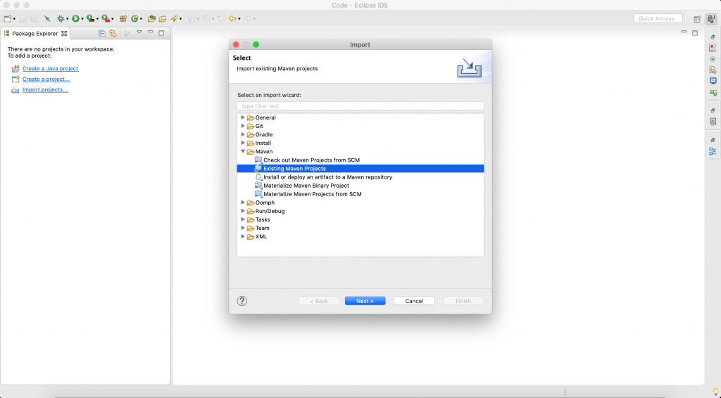
   1. Open Eclipse IDE. Select File -> Import.
      A dialog box will open, as shown in Figure 2.

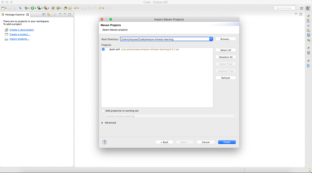
2. Select Maven -> Existing Maven Projects, and select Next. Then you will be prompted to select a folder location for stock trader application.

Select Browse, and navigate to the downloaded source code folder location. The IDE will automatically detect maven pom.xml.

Select Finish to complete the import. IDE will take 2–3 minutes to download all libraries to complete setup stock trader project.

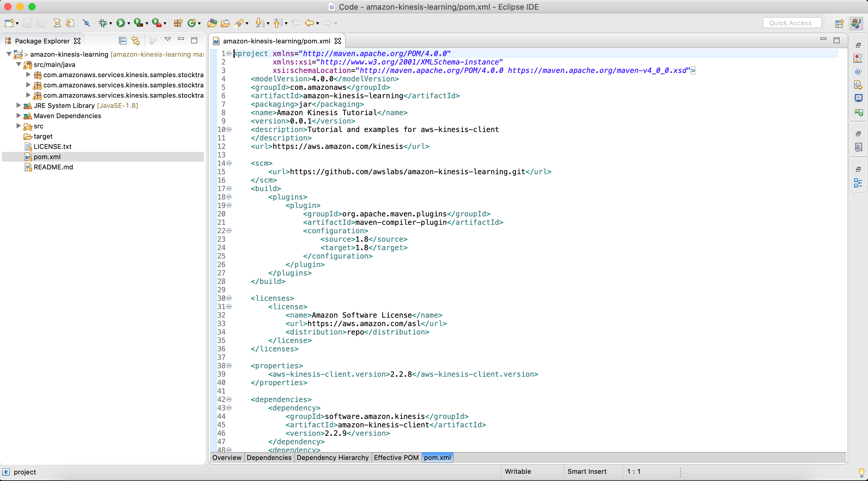
3. After the setup is complete, the IDE will look like similar to Figure 4.

4. Open pom.xml, and replace it with the following content. This will add all the prerequisites and dependencies required to build and package the jar application.

<project xmlns="http://maven.apache.org/POM/4.0.0"
         xmlns:xsi="http://www.w3.org/2001/XMLSchema-instance"
         xsi:schemaLocation="http://maven.apache.org/POM/4.0.0 https://maven.apache.org/maven-v4_0_0.xsd">
    <modelVersion>4.0.0</modelVersion>
    <groupId>com.amazonaws</groupId>
    <artifactId>amazon-kinesis-learning</artifactId>
    <packaging>jar</packaging>
    <name>Amazon Kinesis Tutorial</name>
    <version>0.0.1</version>
    <description>Tutorial and examples for aws-kinesis-client
    </description>
    <url>https://aws.amazon.com/kinesis</url>

    <scm>
        <url>https://github.com/awslabs/amazon-kinesis-learning.git</url>
    </scm>

    <licenses>
        <license>
            <name>Amazon Software License</name>
            <url>https://aws.amazon.com/asl</url>
            <distribution>repo</distribution>
        </license>
    </licenses>

    <properties>
        <aws-kinesis-client.version>2.3.4</aws-kinesis-client.version>
    </properties>

    <dependencies>
        <dependency>
            <groupId>software.amazon.kinesis</groupId>
            <artifactId>amazon-kinesis-client</artifactId>
            <version>2.3.4</version>
        </dependency>
        <dependency>
            <groupId>commons-logging</groupId>
            <artifactId>commons-logging</artifactId>
            <version>1.2</version>
        </dependency>
		<dependency>
		    <groupId>software.amazon.awssdk</groupId>
		    <artifactId>sts</artifactId>
		    <version>2.16.74</version>
		</dependency>
		<dependency>
       <groupId>org.slf4j</groupId>
       <artifactId>slf4j-simple</artifactId>
       <version>1.7.25</version>
   </dependency>
    </dependencies>

 	<build>
        <finalName>amazon-kinesis-learning</finalName>
        <plugins>

            <plugin>
                <groupId>org.apache.maven.plugins</groupId>
                <artifactId>maven-compiler-plugin</artifactId>
                <version>3.6.1</version>
                <configuration>
                    <source>1.8</source>
                    <target>1.8</target>
                </configuration>
            </plugin>

            <plugin>
                <groupId>org.apache.maven.plugins</groupId>
                <artifactId>maven-assembly-plugin</artifactId>
                <version>3.1.1</version>

                <configuration>
                    <descriptorRefs>
                        <descriptorRef>jar-with-dependencies</descriptorRef>
                    </descriptorRefs>
                </configuration>

                <executions>
                    <execution>
                        <id>make-assembly</id>
                        <phase>package</phase>
                        <goals>
                            <goal>single</goal>
                        </goals>
                    </execution>
                </executions>
    
            </plugin>
        </plugins>
    </build>


</project>

Update the main class of consumer application

The updated code for the StockTradesProcessor.java class is shown as follows. The changes made to the class to enable cross-account access are highlighted in bold.

package com.amazonaws.services.kinesis.samples.stocktrades.processor;

import java.util.UUID;
import java.util.logging.Level;
import java.util.logging.Logger;

import org.apache.commons.logging.Log;
import org.apache.commons.logging.LogFactory;

import software.amazon.awssdk.auth.credentials.AwsCredentialsProvider;
import software.amazon.awssdk.regions.Region;
import software.amazon.awssdk.services.dynamodb.DynamoDbAsyncClient;
import software.amazon.awssdk.services.cloudwatch.CloudWatchAsyncClient;
import software.amazon.awssdk.services.kinesis.KinesisAsyncClient;
import software.amazon.awssdk.services.sts.StsClient; import software.amazon.awssdk.services.sts.auth.StsAssumeRoleCredentialsProvider; import software.amazon.awssdk.services.sts.model.AssumeRoleRequest;
import software.amazon.kinesis.common.ConfigsBuilder;
import software.amazon.kinesis.common.KinesisClientUtil;
import software.amazon.kinesis.coordinator.Scheduler;

/**
 * Uses the Kinesis Client Library (KCL) 2.2.9 to continuously consume and process stock trade
 * records from the stock trades stream. KCL monitors the number of shards and creates
 * record processor instances to read and process records from each shard. KCL also
 * load balances shards across all the instances of this processor.
 *
 */
public class StockTradesProcessor {

    private static final Log LOG = LogFactory.getLog(StockTradesProcessor.class);

    private static final Logger ROOT_LOGGER = Logger.getLogger("");
    private static final Logger PROCESSOR_LOGGER =
            Logger.getLogger("com.amazonaws.services.kinesis.samples.stocktrades.processor.StockTradeRecordProcessor");

    private static void checkUsage(String[] args) {
        if (args.length != 5) {
            System.err.println("Usage: " + StockTradesProcessor.class.getSimpleName()
                    + " <application name> <stream name> <region> <role arn> <role session name>");
            System.exit(1);
        }
    }

    /**
     * Sets the global log level to WARNING and the log level for this package to INFO,
     * so that we only see INFO messages for this processor. This is just for the purpose
     * of this tutorial, and should not be considered as best practice.
     *
     */
    private static void setLogLevels() {
        ROOT_LOGGER.setLevel(Level.WARNING);
        // Set this to INFO for logging at INFO level. Suppressed for this example as it can be noisy.
        PROCESSOR_LOGGER.setLevel(Level.WARNING);
    }
    
    private static AwsCredentialsProvider roleCredentialsProvider(String roleArn, String roleSessionName, Region region) { AssumeRoleRequest assumeRoleRequest = AssumeRoleRequest.builder() .roleArn(roleArn) .roleSessionName(roleSessionName) .durationSeconds(900) .build(); LOG.warn("Initializing assume role request session: " + assumeRoleRequest.roleSessionName()); StsClient stsClient = StsClient.builder().region(region).build(); StsAssumeRoleCredentialsProvider stsAssumeRoleCredentialsProvider = StsAssumeRoleCredentialsProvider .builder() .stsClient(stsClient) .refreshRequest(assumeRoleRequest) .asyncCredentialUpdateEnabled(true) .build(); LOG.warn("Initializing sts role credential provider: " + stsAssumeRoleCredentialsProvider.prefetchTime().toString()); return stsAssumeRoleCredentialsProvider; }

    public static void main(String[] args) throws Exception {
        checkUsage(args);

        setLogLevels();

        String applicationName = args[0];
        String streamName = args[1];
        Region region = Region.of(args[2]);
        String roleArn = args[3]; String roleSessionName = args[4]; 
        
        if (region == null) {
            System.err.println(args[2] + " is not a valid AWS region.");
            System.exit(1);
        }
        
        AwsCredentialsProvider awsCredentialsProvider = roleCredentialsProvider(roleArn,roleSessionName, region); KinesisAsyncClient kinesisClient = KinesisClientUtil.createKinesisAsyncClient(KinesisAsyncClient.builder().region(region).credentialsProvider(awsCredentialsProvider));
        DynamoDbAsyncClient dynamoClient = DynamoDbAsyncClient.builder().region(region).build();
        CloudWatchAsyncClient cloudWatchClient = CloudWatchAsyncClient.builder().region(region).build();
        StockTradeRecordProcessorFactory shardRecordProcessor = new StockTradeRecordProcessorFactory();
        ConfigsBuilder configsBuilder = new ConfigsBuilder(streamName, applicationName, kinesisClient, dynamoClient, cloudWatchClient, UUID.randomUUID().toString(), shardRecordProcessor);

        Scheduler scheduler = new Scheduler(
                configsBuilder.checkpointConfig(),
                configsBuilder.coordinatorConfig(),
                configsBuilder.leaseManagementConfig(),
                configsBuilder.lifecycleConfig(),
                configsBuilder.metricsConfig(),
                configsBuilder.processorConfig(),
                configsBuilder.retrievalConfig()
        );
        int exitCode = 0;
        try {
            scheduler.run();
        } catch (Throwable t) {
            LOG.error("Caught throwable while processing data.", t);
            exitCode = 1;
        }
        System.exit(exitCode);

    }

}

Let’s review the changes made to the code to understand the key parts of how the cross-account access works.

AssumeRoleRequest assumeRoleRequest = AssumeRoleRequest.builder() .roleArn(roleArn) .roleSessionName(roleSessionName) .durationSeconds(900) .build();

AssumeRoleRequest class is used to get the credentials to access the Kinesis data stream in Account A using the role that was created. The value of the variable assumeRoleRequest is passed to the StsAssumeRoleCredentialsProvider.

StsClient stsClient = StsClient.builder().region(region).build();

StsAssumeRoleCredentialsProvider stsAssumeRoleCredentialsProvider = StsAssumeRoleCredentialsProvider .builder() .stsClient(stsClient) .refreshRequest(assumeRoleRequest) .asyncCredentialUpdateEnabled(true) .build();

StsAssumeRoleCredentialsProvider periodically sends an AssumeRoleRequest to the AWS STS to maintain short-lived sessions to use for authentication. Using refreshRequest, these sessions are updated asynchronously in the background as they get close to expiring. As asynchronous refresh is not set by default, we explicitly set it to true using asyncCredentialUpdateEnabled.

AwsCredentialsProvider awsCredentialsProvider = roleCredentialsProvider(roleArn,roleSessionName, region);

KinesisAsyncClient kinesisClient = KinesisClientUtil.createKinesisAsyncClient(KinesisAsyncClient.builder().region(region).credentialsProvider(awsCredentialsProvider));

• KinesisAsyncClient is the client for accessing Kinesis asynchronously. We can create an instance of KinesisAsyncClient by passing to it the credentials to access the Kinesis data stream in Account A through the assume role. The values of Kinesis, DynamoDB, and the CloudWatch client along with the stream name, application name is used to create a ConfigsBuilder instance.
• The ConfigsBuilder instance is used to create the KCL scheduler (also known as KCL worker in KCL versions 1.x).
• The scheduler creates a new thread for each shard (assigned to this consumer instance), which continuously loops to read records from the data stream. It then invokes the record processor instance (StockTradeRecordProcessor in this example) to process each batch of records received. This is the class which will contain your record processing logic. The Developing Custom Consumers with Shared Throughput Using KCL section of the documentation will provide more details on the working of KCL.

KCL application in python

In this section we will show you how to configure a KCL application written in Python to access a cross-account Kinesis data stream.

A.      Steps 1 and 2 from earlier remain the same and will need to be completed before moving ahead. After the IAM roles and policies have been created, log into the EC2 instance and clone the amazon-kinesis-client-python repository using the following command.

git clone https://github.com/awslabs/amazon-kinesis-client-python.git

B.      Navigate to the amazon-kinesis-client-python directory and run the following commands.

sudo yum install python-pip
sudo pip install virtualenv
virtualenv /tmp/kclpy-sample-env
source /tmp/kclpy-sample/env/bin/activate
pip install amazon_kclpy

C.      Next, navigate to amazon-kinesis-client-python/samples and open the sample.properties file. The properties file has properties such as streamName, application name, and credential information that lets you customize the configuration for your use case.

D.      We will modify the properties file to change the stream name and application name, and to add the credentials to enable access to a Kinesis data stream in a different account. You can replace the sample.properties file and replace with the following snippet. The bolded sections show the changes we have made.

# The script that abides by the multi-language protocol. This script will

# be executed by the MultiLangDaemon, which will communicate with this script

# over STDIN and STDOUT according to the multi-language protocol.

executableName = sample_kclpy_app.py

# The name of an Amazon Kinesis stream to process.

streamName = StockTradeStream

# Used by the KCL as the name of this application. Will be used as the name

# of an Amazon DynamoDB table which will store the lease and checkpoint

# information for workers with this application name

applicationName = StockTradesProcessor

# Users can change the credentials provider the KCL will use to retrieve credentials.

# The DefaultAWSCredentialsProviderChain checks several other providers, which is

# described here:

# http://docs.aws.amazon.com/AWSJavaSDK/latest/javadoc/com/amazonaws/auth/DefaultAWSCredentialsProviderChain.html

#AWSCredentialsProvider = DefaultAWSCredentialsProviderChain

AWSCredentialsProvider = STSAssumeRoleSessionCredentialsProvider|arn:aws:iam::Account-A-AccountNumber:role/kds-stock-trade-stream-role|kinesiscrossaccount

AWSCredentialsProviderDynamoDB = DefaultAWSCredentialsProviderChain

AWSCredentialsProviderCloudWatch = DefaultAWSCredentialsProviderChain

# Appended to the user agent of the KCL. Does not impact the functionality of the

# KCL in any other way.

processingLanguage = python/2.7

# Valid options at TRIM_HORIZON or LATEST.

# See http://docs.aws.amazon.com/kinesis/latest/APIReference/API_GetShardIterator.html#API_GetShardIterator_RequestSyntax

initialPositionInStream = LATEST

# The following properties are also available for configuring the KCL Worker that is created

# by the MultiLangDaemon.

# The KCL defaults to us-east-1

#regionName = us-east-1

In the above step, you will have to replace Account-A-AccountNumber with the AWS account number of the account that has the kinesis stream.

We use the STSAssumeRoleSessionCredentialsProvider class and pass to it the role created in Account A which have permissions to access the Kinesis data stream. This gives the KCL application in Account B permissions to read the Kinesis data stream in Account A. The DynamoDB lease table and the CloudWatch metrics are in Account B. Hence, we can use the DefaultAWSCredentialsProviderChain for AWSCredentialsProviderDynamoDB and AWSCredentialsProviderCloudWatch in the properties file. You can now save the sample.properties file.

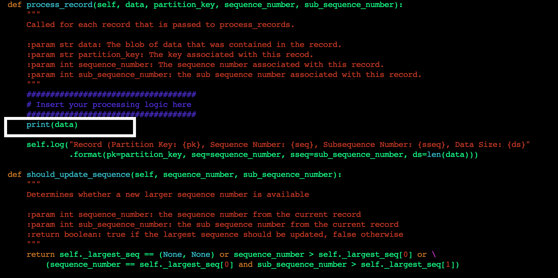
E.      Next, we will change the application code to print the data read from the Kinesis data stream to standard output (STDOUT). Edit the sample_kclpy_app.py under the samples directory. You will add all your application code logic in the process_record method. This method is called for every record in the Kinesis data stream. For this blog post, we will add a single line to the method to print the records to STDOUT, as shown in Figure 5.

F.       Save the file, and run the following command to build the project with the changes you just made.

cd amazon-kinesis-client-python/
python setup.py install

G.     Now you are ready to run the application. To start the KCL application, run the following command from the amazon-kinesis-client-python directory.

`amazon_kclpy_helper.py --print_command --java /usr/bin/java --properties samples/sample.properties`

This will start the application. Your application is now ready to read the data from the Kinesis data stream in another account and display the contents of the stream on STDOUT. When the producer starts writing data to the Kinesis data stream in Account A, you will start seeing those results being printed.

Clean Up

Once you are done testing the cross-account access make sure you clean up your environment to avoid incurring cost. As part of the cleanup we recommend you delete the Kinesis data stream, StockTradeStream, the EC2 instances that the KCL application is running on, and the DynamoDB table that was created by the KCL application.

Conclusion

In this blog post, we discussed the techniques to configure your KCL applications written in Java and Python to access a Kinesis data stream in a different AWS account. We also provided sample code and configurations which you can modify and use in your application code to set up the cross-account access. Now you can continue to build a multi-account strategy on AWS, while being able to easily access your Kinesis data streams from applications in multiple AWS accounts.