Tag Archives: Customer Solutions

Analyze logs with Dynatrace Davis AI Engine using Amazon Kinesis Data Firehose HTTP endpoint delivery

Post Syndicated from Erick Leon original https://aws.amazon.com/blogs/big-data/analyze-logs-with-dynatrace-davis-ai-engine-using-amazon-kinesis-data-firehose-http-endpoint-delivery/

This blog post is co-authored with Erick Leon, Sr. Technical Alliance Manager from Dynatrace.

Amazon Kinesis Data Firehose is the easiest way to reliably load streaming data into data lakes, data stores, and analytics services. With just a few clicks, you can create fully-managed delivery streams that auto scale on demand to match the throughput of your data. Customers already use Kinesis Data Firehose to ingest raw data from various data sources, including logs from AWS services. Kinesis Data Firehose now supports delivering streaming data to Dynatrace. Dynatrace begins analyzing incoming data within minutes of Amazon CloudWatch data generation.

Starting today, you can use Kinesis Data Firehose to send CloudWatch Metrics and Logs directly to the Dynatrace observability platform to perform your explorations and analysis. Dynatrace, an AWS Partner Network (APN) has provided full observability into AWS Services by ingesting CloudWatch metrics that are published by AWS services. Dynatrace ingests this data to perform root-cause analysis using the Dynatrace Davis AI engine.

In this post, we describe the Kinesis Data Firehose and related Dynatrace integration.

Prerequisites

For this walkthrough, you should have the following prerequisites:

  • AWS account.
  • Access to the CloudWatch and Kinesis Data Firehose with permissions to manage HTTP endpoints.
  • Dynatrace Intelligent Observability Platform account, or get a free 15 day trial here.
  • Dynatrace version 1.182+.
  • An updated AWS monitoring policy to include the additional AWS services.
    To update the AWS Identity and Access Management (IAM) policy, use the JSON in the link above, containing the monitoring policy (permissions) for all supporting services.
  • Dynatrace API token: create token with the following permission and keep readily available in a notepad.
Dynatrace API Token

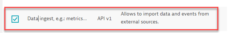
Figure 1 – Dynatrace API Token

How it works

Amazon Kinesis Data Firehose HTTP endpoint delivery

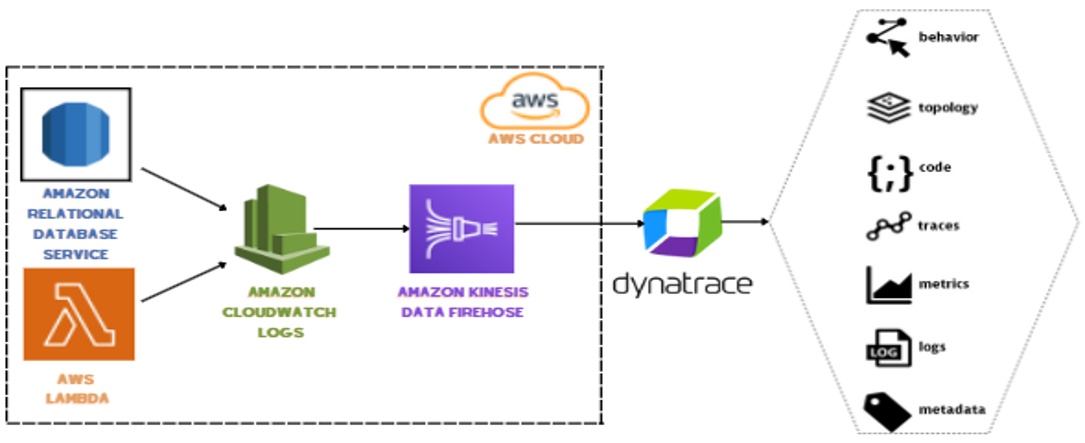
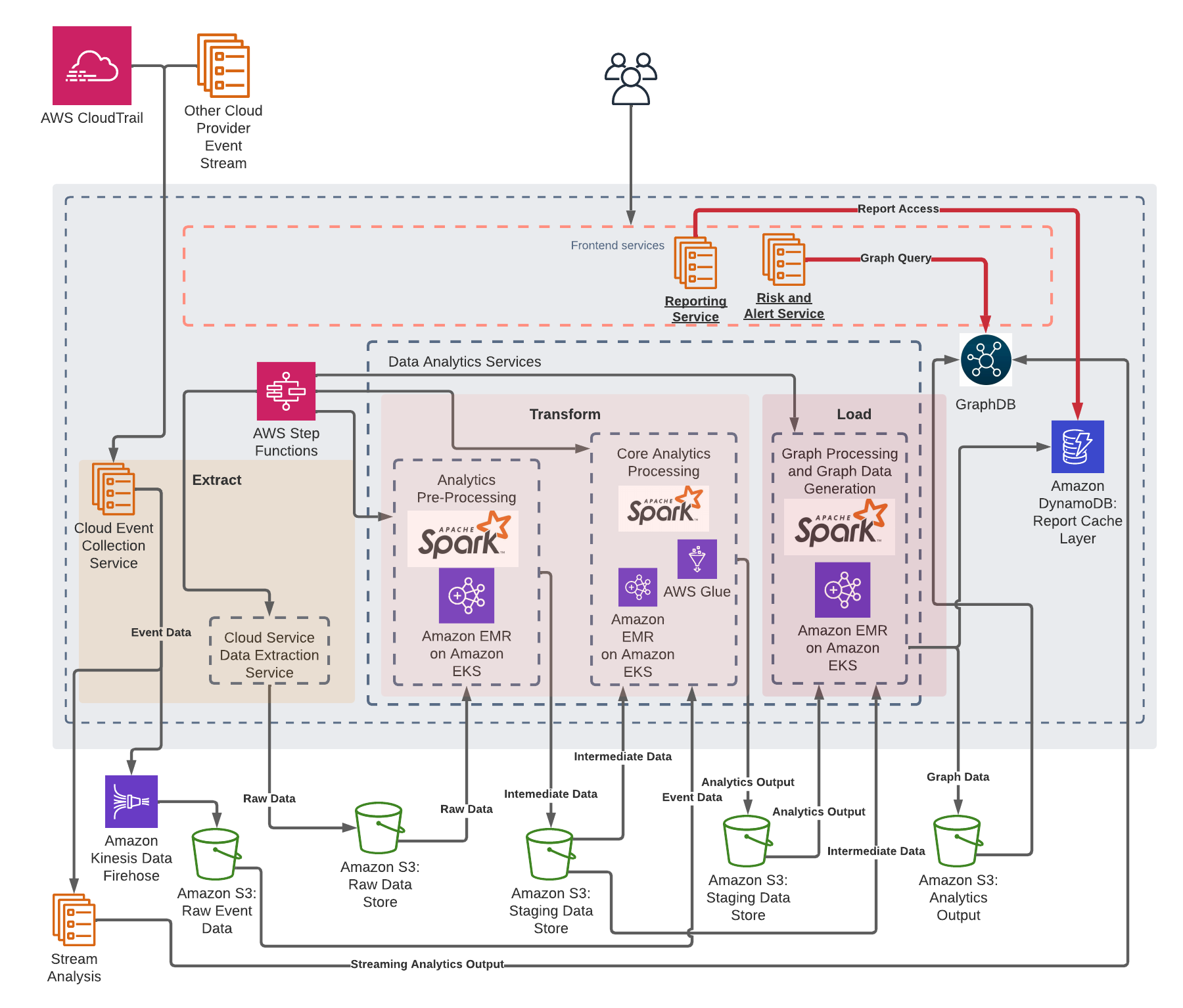
Figure 2 – Amazon Kinesis Data Firehose HTTP endpoint delivery

Simply create a log stream for your Amazon services to deliver your context rich logs to the Amazon CloudWatch Logs service. Next, select your Dynatrace HTTP endpoint to enhance your logs streams with the power of the Dynatrace Intelligence Platform. Finally, you can also back up your logs to an Amazon Simple Storage Service (Amazon S3) bucket.

Setup instructions

To add a service to monitoring, follow these steps:

  1. In the Dynatrace menu, go to Settings > Cloud and virtualization, and select AWS.
  2. On the AWS overview page, scroll down and select the desired AWS instance. Select the Edit button.
  3. Scroll down and select Add service. Choose the service name from the drop-down, and select Add service.
  4. Select Save changes.

To process and deliver AWS CloudWatch Metrics to Dynatrace, follow these steps.

  1. Log in to the AWS console and type “Kinesis” in the text search bar. Select Kinesis
AWS Console

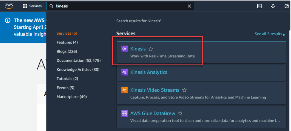
Figure 3 – AWS Console

  1. On the Amazon Kinesis services page, select the radio button for Kinesis Data Firehose and select the Create delivery stream button.
Amazon Kinesis

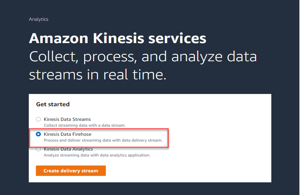
Figure 4 – Amazon Kinesis

  1. Choose the “Direct PUT” from the drop down, and from Destination drop down, choose “Dynatrace”.
Amazon Kinesis Data Firehose

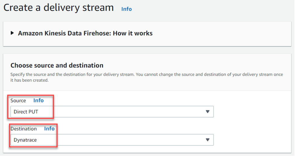
Figure 5 – Amazon Kinesis Data Firehose

  1. Delivery stream name – Give your stream a new name, for example: – “KFH-StreamToDynatrace”

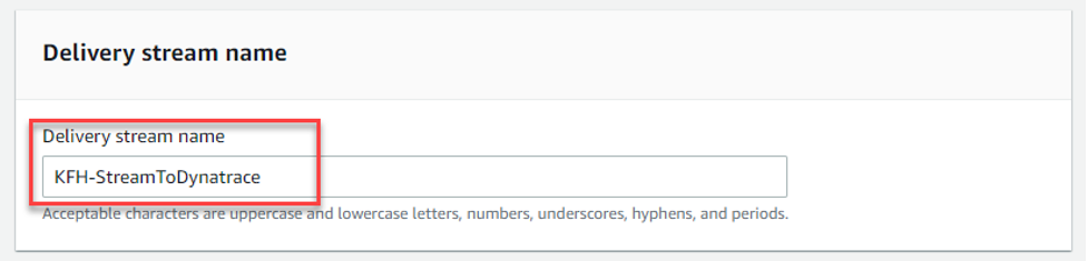
Figure 6 – Delivery stream name

  1. In the section “Destination settings”:
Destination settings

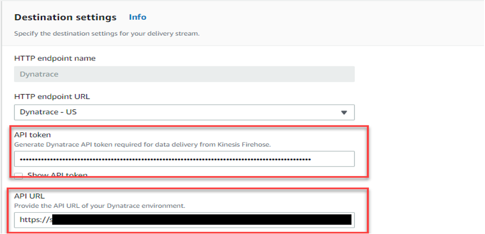
Figure 7 – Destination settings

  1. HTTP endpoint name – “Dynatrace”.
  2. HTTP endpoint URL – From the drop down, select “Dynatrace – US”.
  3. API token – Enter Dynatrace API TOKEN created in the prerequisite section.
  4. API URL – enter the Dynatrace URL for your tenant, for example: https://xxxxx.live.dynatrace.com
  5. Back Up Settings – Either select an existing S3 bucket or create a new one and add details and select the Create delivery stream button.
Backup settings

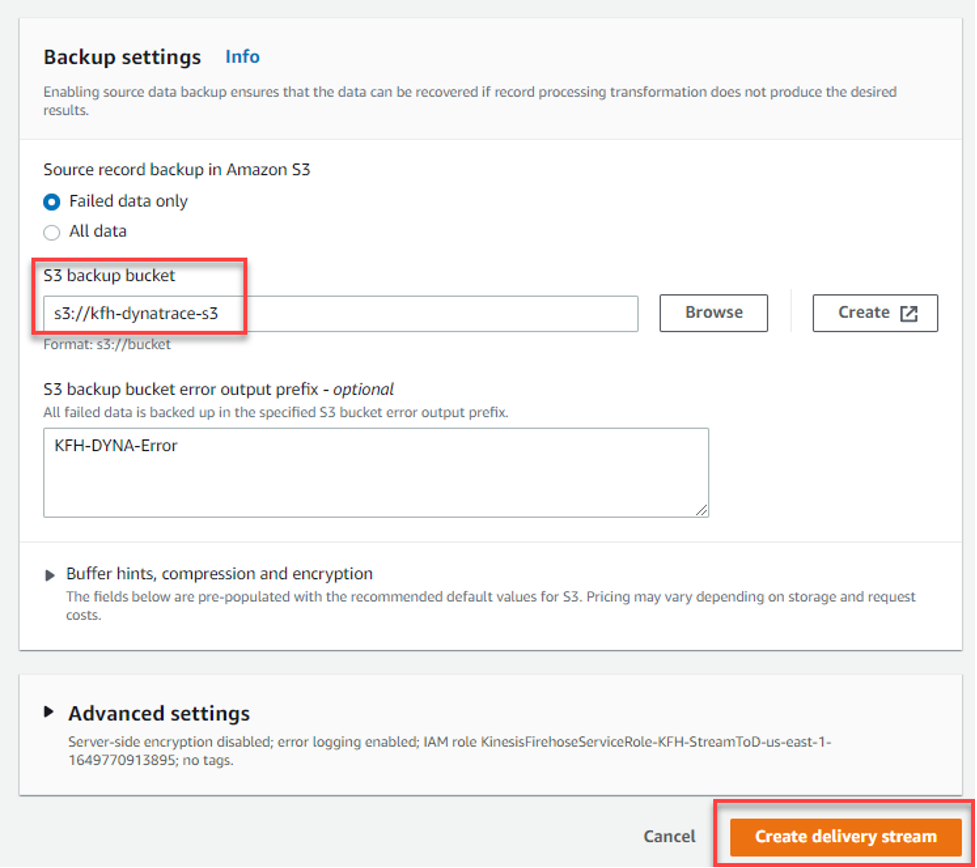
Figure 8 – Backup settings

Once successful, your AWS Console will look like the following:

Amazon Kinesis Data Firehose

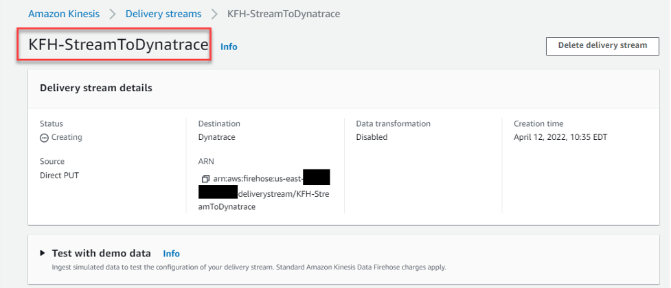
Figure 9 – Amazon Kinesis Data Firehose

The Dynatrace Experience

Once the initial setups are completed in both Dynatrace and the AWS Console, follow these steps to visualize your new KHF stream data in the Dynatrace console.

  1. Log in to the Dynatrace Console, and on the left side menu expand the “infrastructure” section, and select “AWS
  2. From the screen, select the AWS account that you want to add the KFH stream to.
  3. Next, you’ll see a virtualization of your AWS assets for the account selected. Select the box marked “Supporting Services”.
  4. Next, press the “Configure services” button.
  5. Next, select “Add service”.
  6. From the drop down, select “Kinesis Data Firehose”.
  7. Next, select the “Add metric” button, and select the metrics that you want to see for this stream. Dynatrace has a comprehensive list of metrics that can be selected from the UI. The list can be found in this link.

Troubleshooting

  1. After configuration, load to the new KFH stream no data in the Dynatrace Console.
    1. Check the Error Logs tab check to make sure that the Destination URL is correct for the Dynatrace Tenant.
Destination error logs

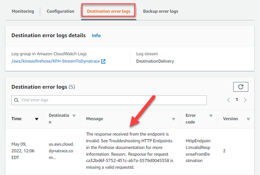
Figure 10 – Destination error logs

  1. Invalid or misconfigured Dynatrace API token or scope isn’t properly set.
Destination error logs

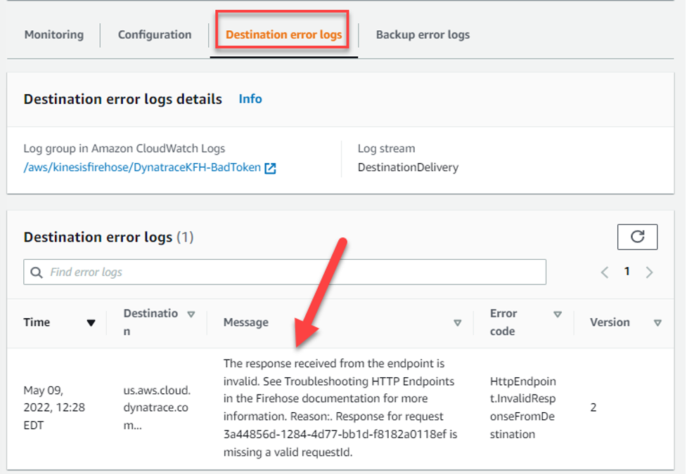
Figure 11 – Destination error logs

Conclusion

In this post, we demonstrate the Kinesis Data Firehose and related Dynatrace integration. In addition, engineers can use CloudWatch Metrics to explore their production systems alongside events in Dynatrace. This provides a seamless, current view of your system (from logs to events and traces) in a single data store.

To learn more about CloudWatch Service, see the Amazon CloudWatch home page. If you have any questions, post them on the AWS CloudWatch service forum.

If you haven’t yet signed up for Dynatrace, then you can try out Kinesis Data Firehose with Dynatrace with a free Dynatrace trial.


About the Authors

Erick Leon is a Technical Alliances Sr. Manager at Dynatrace, Observability Practice Architect, and Customer Advocate. He promotes strong technical integrations with a focus on AWS. With over 15 years as a Dynatrace customer, his real-world experiences and lessons learned bring valuable insights into the Dynatrace Intelligent Observability Platform.

Shashiraj Jeripotula (Raj) is a San Francisco-based Sr. Partner Solutions Architect at AWS. He works with various independent software vendors (ISVs), and partners who specialize in cloud management tools and DevOps to develop joint solutions and accelerate cloud adoption on AWS.

How William Hill migrated NoSQL workloads at scale to Amazon Keyspaces

Post Syndicated from Kunal Gautam original https://aws.amazon.com/blogs/big-data/how-william-hill-migrated-nosql-workloads-at-scale-to-amazon-keyspaces/

Social gaming and online sports betting are competitive environments. The game must be able to handle large volumes of unpredictable traffic while simultaneously promising zero downtime. In this domain, user retention is no longer just desirable, it’s critical. William Hill is a global online gambling company based in London, England, and it is the founding member of the UK Betting and Gaming Council. They share the mission to champion the betting and gaming industry and set world-class standards to make sure of an enjoyable, fair, and safe betting and gambling experience for all of their customers. In sports betting, William Hill is an industry-leading brand, awarded with prestigious industry titles like the IGA Awards Sports Betting Operator of the year in 2019, 2020, and 2022, and the SBC Awards Racing Sportsbook of the Year in 2019. William Hill has been acquired by Caesars Entertainment, Inc (NASDAQ: CZR) in April 2021, and it’s the largest casino-entertainment company in the US and one of the world’s most diversified casino-entertainment providers. At the heart of William Hill gaming platform is a NoSQL database that maintains 100% uptime, scales in real-time to handle millions of users or more, and provides users with a responsive and personalized experience across all of their devices.

In this post, we’ll discuss how William Hill moved their workload from Apache Cassandra to Amazon Keyspaces (for Apache Cassandra) with zero downtime using AWS Glue ETL.

William Hill was facing challenges regarding scalability, cluster instability, high operational costs, and manual patching and server maintenance. They were looking for a NoSQL solution which was scalable, highly-available, and completely managed. This let them focus on providing better user experience rather than maintaining infrastructure. William Hill Limited decided to move forward with Amazon Keyspaces, since it can run Apache Cassandra workloads on AWS using the same Cassandra application code and developer tools used today, without the need to provision, patch, manage servers, install, maintain, or operate software.

Solution overview

William Hill Limited wanted to migrate their existing Apache Cassandra workloads to Amazon Keyspaces with a replication lag of minutes, with minimum migration costs and development efforts. Therefore, AWS Glue ETL was leveraged to deliver the desired outcome.

AWS Glue is a serverless data integration service that provides multiple benefits for migration:

  • No infrastructure to maintain; allocates the necessary computing power and runs multiple migration jobs simultaneously.
  • All-in-one pricing model that includes infrastructure and is 55% cheaper than other cloud data integration options.
  • No lock in with the service; possible to develop data migration pipelines in open-source Apache Spark (Spark SQL, PySpark, and Scala).
  • Migration pipeline can be scaled fearlessly with Amazon Keyspaces and AWS Glue.
  • Built-in pipeline monitoring to make sure of in-migration continuity.
  • AWS Glue ETL jobs make it possible to perform bulk data extraction from Apache Cassandra and ingest to Amazon Keyspaces.

In this post, we’ll take you through William Hill’s journey of building the migration pipeline from scratch to migrate the Apache Cassandra workload to Amazon Keyspaces by leveraging AWS Glue ETL with DataStax Spark Cassandra connector.

For the purpose of this post, let’s look at a typical Cassandra Network setup on AWS and the mechanism used to establish the connection with AWS Glue ETL. The migration solution described also works for Apache Cassandra hosted on on-premises clusters.

Architecture overview

The architecture demonstrates the migration environment that requires Amazon Keyspaces, AWS Glue, Amazon Simple Storage Service (Amazon S3), and the Apache Cassandra cluster. To avoid a high CPU utilization/saturation on the Apache Cassandra cluster during the migration process, you might want to deploy another Cassandra datacenter to isolate your production from the migration workload to make the migration process seamless for your customers.

Amazon S3 has been used for staging while migrating data from Apache Cassandra to Amazon Keyspaces to make sure that the IO load on Cassandra serving live traffic on production is minimized, in case the data upload to Amazon Keyspaces fails and a retry must be done.

Prerequisites

The Apache Cassandra cluster is hosted on Amazon Elastic Compute Cloud (Amazon EC2) instances, spread across three availability zones, and hosted in private subnets. AWS Glue ETL is hosted on Amazon Virtual Private Cloud (Amazon VPC) and thus needs a AWS Glue Studio custom Connectors and Connections to be setup to communicate with the Apache Cassandra nodes hosted on the private subnets in the customer VPC. Thereby, this enables the connection to the Cassandra cluster hosted in the VPC. The DataStax Spark Cassandra Connector must be downloaded and saved onto an Amazon S3 bucket: s3://$MIGRATION_BUCKET/jars/spark-cassandra-connector-assembly_2.12-3.2.0.jar.

Let’s create an AWS Glue Studio custom connector named cassandra_connection and its corresponding connection named conn-cassandra-custom for AWS region us-east-1.

For the connector created, create an AWS Glue Studio connection and populate it with network information VPC, and a Subnet allowing for AWS Glue ETL to establish a connection with Apache Casandra.

  • Name: conn-cassandra-custom
  • Network Options

Let’s begin by creating a keyspace and table in Amazon Keyspaces using Amazon Keyspaces Console or CQLSH, and then create a target keyspace named target_keyspace and a target table named target_table.

CREATE KEYSPACE target_keyspace WITH replication = {'class': 'SingleRegionStrategy'};

CREATE TABLE target_keyspace.target_table (
    userid      uuid,
    level       text,
    gameid      int,
    description text,
    nickname    text,
    zip         text,
    email       text,
    updatetime  text,
    PRIMARY KEY (userid, level, gameid)
) WITH default_time_to_live = 0 AND CUSTOM_PROPERTIES = {
	'capacity_mode':{
		'throughput_mode':'PROVISIONED',
		'write_capacity_units':76388,
		'read_capacity_units':3612
	}
} AND CLUSTERING ORDER BY (level ASC, gameid ASC);

After the table has been created, switch the table to on-demand mode to pre-warm the table and avoid AWS Glue ETL job throttling failures. The following script will update the throughput mode.

ALTER TABLE target_keyspace.target_table 
WITH CUSTOM_PROPERTIES = {
	'capacity_mode':{
		'throughput_mode':'PAY_PER_REQUEST'
	}
} 

Let’s go ahead and create two Amazon S3 buckets to support the migration process. The first bucket (s3://your-spark-cassandra-connector-bucket-name)should store the spark Cassandra connector assembly jar file, Cassandra, and Keyspaces configuration YAML files.

The second bucket (s3://your-migration-stage-bucket-name) will be used to store intermediate parquet files to identify the delta between the Cassandra cluster and the Amazon Keyspaces table to track changes between subsequent executions of the AWS Glue ETL jobs.

In the following KeyspacesConnector.conf, set your contact points to connect to Amazon Keyspaces, and replace the username and the password to the AWS credentials.

Using the RateLimitingRequestThrottler we can make sure that requests don’t exceed the configured Keyspaces capacity. The G1.X DPU creates one executor per worker. The RateLimitingRequestThrottler in this example is set for 1000 requests per second. With this configuration, and G.1X DPU, you’ll achieve 1000 request per AWS Glue worker. Adjust the max-requests-per-second accordingly to fit your workload. Increase the number of workers to scale throughput to a table.

datastax-java-driver {
  basic.request.consistency = "LOCAL_QUORUM"
  basic.contact-points = ["cassandra.us-east-1.amazonaws.com:9142"]
   advanced.reconnect-on-init = true
   basic.load-balancing-policy {
        local-datacenter = "us-east-1"
    }
    advanced.auth-provider = {
       class = PlainTextAuthProvider
       username = "user-at-sample"
       password = "S@MPLE=PASSWORD="
    }
    advanced.throttler = {
       class = RateLimitingRequestThrottler
       max-requests-per-second = 1000
       max-queue-size = 50000
       drain-interval = 1 millisecond
    }
    advanced.ssl-engine-factory {
      class = DefaultSslEngineFactory
      hostname-validation = false
    }
    advanced.connection.pool.local.size = 1
}

Similarly, create a CassandraConnector.conf file, set the contact points to connect to the Cassandra cluster, and replace the username and the password respectively.

datastax-java-driver {
  basic.request.consistency = "LOCAL_QUORUM"
  basic.contact-points = ["127.0.0.1:9042"]
   advanced.reconnect-on-init = true
   basic.load-balancing-policy {
        local-datacenter = "datacenter1"
    }
    advanced.auth-provider = {
       class = PlainTextAuthProvider
       username = "user-at-sample"
       password = "S@MPLE=PASSWORD="
    }
}

Build AWS Glue ETL migration pipeline with Amazon Keyspaces

To build reliable, consistent delta upload Glue ETL pipeline, let’s decouple the migration process into two AWS Glue ETLs.

  • CassandraToS3 Glue ETL: Read data from the Apache Cassandra cluster and transfer the migration workload to Amazon S3 in the Apache Parquet format. To identify incremental changes in the Cassandra tables, the job stores separate parquet files with primary keys with an updated timestamp.
  • S3toKeyspaces Glue ETL: Uploads the migration workload from Amazon S3 to Amazon Keyspaces. During the first run, the ETL uploads the complete data set from Amazon S3 to Amazon Keyspaces, and for the subsequent run calculates the incremental changes by comparing the updated timestamp across two subsequent runs and calculating the incremental difference. The job also takes care of inserting new records, updating existing records, and deleting records based on the incremental difference.

In this example, we’ll use Scala to write the AWS Glue ETL, but you can also use PySpark.

Let’s go ahead and create an AWS Glue ETL job named CassandraToS3 with the following job parameters:

aws glue create-job \
    --name "CassandraToS3" \
    --role "GlueKeyspacesMigration" \
    --description "Offload data from the Cassandra to S3" \
    --glue-version "3.0" \
    --number-of-workers 2 \
    --worker-type "G.1X" \
    --connections "conn-cassandra-custom" \
    --command "Name=glueetl,ScriptLocation=s3://$MIGRATION_BUCKET/scripts/CassandraToS3.scala" \
    --max-retries 0 \
    --default-arguments '{
        "--job-language":"scala",
        "--KEYSPACE_NAME":"source_keyspace",
        "--TABLE_NAME":"source_table",
        "--S3_URI_FULL_CHANGE":"s3://$MIGRATION_BUCKET/full-dataset/",
        "--S3_URI_CURRENT_CHANGE":"s3://$MIGRATION_BUCKET/incremental-dataset/current/",
        "--S3_URI_NEW_CHANGE":"s3://$MIGRATION_BUCKET/incremental-dataset/new/",
        "--extra-files":"s3://$MIGRATION_BUCKET/conf/CassandraConnector.conf",
        "--conf":"spark.cassandra.connection.config.profile.path=CassandraConnector.conf",
        "--class":"GlueApp"
    }'

The CassandraToS3 Glue ETL job reads data from the Apache Cassandra table source_keyspace.source_table and writes it to the S3 bucket in the Apache Parquet format. The job rotates the parquet files to help identify delta changes in the data between consecutive job executions. To identify inserts, updates, and deletes, you must know primary key and columns write times (updated timestamp) in the Cassandra cluster up front. Our primary key consists of several columns userid, level, gameid, and a write time column updatetime. If you have multiple updated columns, then you must use more than one write time columns with an aggregation function. For example, for email and updatetime, take the maximum value between write times for email and updatetime.

The following AWS Glue spark code offloads data to Amazon S3 using the spark-cassandra-connector. The script takes four parameters KEYSPACE_NAME, KEYSPACE_TABLE, S3_URI_CURRENT_CHANGE, S3_URI_CURRENT_CHANGE, and S3_URI_NEW_CHANGE.

To upload the data from Amazon S3 to Amazon Keyspaces, you must create a S3toKeyspaces Glue ETL job using the Glue spark code to read the parquet files from the Amazon S3 bucket created as an output of CassandraToS3 Glue job and identify inserts, updates, deletes, and execute requests against the target table in Amazon Keyspaces. The code sample provided takes four parameters: KEYSPACE_NAME, KEYSPACE_TABLE, S3_URI_CURRENT_CHANGE, S3_URI_CURRENT_CHANGE, and S3_URI_NEW_CHANGE.

Let’s go ahead and create our second AWS Glue ETL job S3toKeyspaces with the following job parameters:

aws glue create-job \
    --name "S3toKeyspaces" \
    --role "GlueKeyspacesMigration" \
    --description "Push data to Amazon Keyspaces" \
    --glue-version "3.0" \
    --number-of-workers 2 \
    --worker-type "G.1X" \
    --command "Name=glueetl,ScriptLocation=s3://amazon-keyspaces-backups/scripts/S3toKeyspaces.scala" \
    --default-arguments '{
        "--job-language":"scala",
        "--KEYSPACE_NAME":"target_keyspace",
        "--TABLE_NAME":"target_table",
        "--S3_URI_FULL_CHANGE":"s3://$MIGRATION_BUCKET/full-dataset/",
        "--S3_URI_CURRENT_CHANGE":"s3://$MIGRATION_BUCKET/incremental-dataset/current/",
        "--S3_URI_NEW_CHANGE":"s3://$MIGRATION_BUCKET/incremental-dataset/new/",
        "--extra-files":"s3://$MIGRATION_BUCKET/conf/KeyspacesConnector.conf",
        "--conf":"spark.cassandra.connection.config.profile.path=KeyspacesConnector.conf",
        "--class":"GlueApp"
    }'

Job scheduling

The final step is to configure AWS Glue Triggers or Amazon EventBridge depending on your scheduling needs to trigger S3toKeyspaces Glue ETL when the job CassandraToS3 has succeeded. If you want to run the CassandraToS3 based on the schedule and configure the schedule option, then the following example showcases how to schedule cassandraToS3 to run every 15 minutes.

Job tuning

There are Spark settings recommended to begin with Amazon Keyspaces, which can then be increased later as appropriate for your workload.

  • Use a Spark partition size (groups multiple Cassandra rows) smaller than 8 MBs to avoid replaying large Spark tasks during a task failure.
  • Use a low concurrent number of writes per DPU with a large number of retries. Add the following options to the job parameters: --conf spark.cassandra.query.retry.count=500 --conf spark.cassandra.output.concurrent.writes=3.
  • Set spark.task.maxFailures to a bounded value. For example, you can start from 32 and increase as needed. This option can help you increase a number of tasks reties during a table pre-warm stage. Add the following option to the job parameters: --conf spark.task.maxFailures=32
  • Another recommendation is to turn off batching to improve random access patterns. Add the following options to the job parameters:
    spark.cassandra.output.batch.size.rows=1
    spark.cassandra.output.batch.grouping.key=none spark.cassandra.output.batch.grouping.buffer.size=100
  • Randomize your workload. Amazon Keyspaces partitions data using partition keys. Although Amazon Keyspaces has built-in logic to help load balance requests for the same partition key, loading the data is faster and more efficient if you randomize the order because you can take advantage of the built-in load balancing of writing to different partitions. To spread the writes across the partitions evenly, you must randomize the data in the dataframe. You might use a rand function to shuffle rows in the dataframe.

Summary

William Hill was able to migrate their workload from Apache Cassandra to Amazon Keyspaces at scale using AWS Glue, without the needs to make any changes on their application tech stack. The adoption of Amazon Keyspaces has provided them with the headroom to focus on their Application and customer experience, as with Amazon Keyspaces there’s no need to manage servers, get performance at scale, highly-scalable, and secure solution with the ability to handle the sudden spike in demand.

In this post, you saw how to use AWS Glue to migrate the Cassandra workload to Amazon Keyspaces, and simultaneously keep your Cassandra source databases completely functional during the migration process. When your applications are ready, you can choose to cut over your applications to Amazon Keyspaces with minimal replication lag in sub minutes between the Cassandra cluster and Amazon Keyspaces. You can also use a similar pipeline to replicate the data back to the Cassandra cluster from Amazon Keyspaces to maintain data consistency, if needed. Here you can find the documents and code to help accelerate your migration to Amazon Keyspaces.


About the Authors

Nikolai Kolesnikov is a Senior Data Architect and helps AWS Professional Services customers build highly-scalable applications using Amazon Keyspaces. He also leads Amazon Keyspaces ProServe customer engagements.

Kunal Gautam is a Senior Big Data Architect at Amazon Web Services. Having experience in building his own Startup and working along with enterprises, he brings a unique perspective to get people, business and technology work in tandem for customers. He is passionate about helping customers in their digital transformation journey and enables them to build scalable data and advance analytics solutions to gain timely insights and make critical business decisions. In his spare time, Kunal enjoys Marathons, Tech Meetups and Meditation retreats.

Understanding the lifecycle of Amazon EC2 Dedicated Hosts

Post Syndicated from Sheila Busser original https://aws.amazon.com/blogs/compute/understanding-the-lifecycle-of-amazon-ec2-dedicated-hosts/

This post is written by Benjamin Meyer, Sr. Solutions Architect, and Pascal Vogel, Associate Solutions Architect.

Amazon Elastic Compute Cloud (Amazon EC2) Dedicated Hosts enable you to run software on dedicated physical servers. This lets you comply with corporate compliance requirements or per-socket, per-core, or per-VM licensing agreements by vendors, such as Microsoft, Oracle, and Red Hat. Dedicated Hosts are also required to run Amazon EC2 Mac Instances.

The lifecycles and states of Amazon EC2 Dedicated Hosts and Amazon EC2 instances are closely connected and dependent on each other. To operate Dedicated Hosts correctly and consistently, it is critical to understand the interplay between Dedicated Hosts and EC2 Instances. In this post, you’ll learn how EC2 instances are reliant on their (dedicated) hosts. We’ll also dive deep into their respective lifecycles, the connection points of these lifecycles, and the resulting considerations.

What is an EC2 instance?

An EC2 instance is a virtual server running on top of a physical Amazon EC2 host. EC2 instances are launched using a preconfigured template called Amazon Machine Image (AMI), which packages the information required to launch an instance. EC2 instances come in various CPU, memory, storage and GPU configurations, known as instance types, to enable you to choose the right instance for your workload. The process of finding the right instance size is known as right sizing. Amazon EC2 builds on the AWS Nitro System, which is a combination of dedicated hardware and the lightweight Nitro hypervisor. The EC2 instances that you launch in your AWS Management Console via Launch Instances are launched on AWS-controlled physical hosts.

What is an Amazon EC2 Bare Metal instance?

Bare Metal instances are instances that aren’t using the Nitro hypervisor. Bare Metal instances provide direct access to physical server hardware. Therefore, they let you run legacy workloads that don’t support a virtual environment, license-restricted business-critical applications, or even your own hypervisor. Workloads on Bare Metal instances continue to utilize AWS Cloud features, such as Amazon Elastic Block Store (Amazon EBS), Elastic Load Balancing (ELB), and Amazon Virtual Private Cloud (Amazon VPC).

What is an Amazon EC2 Dedicated Host?

An Amazon EC2 Dedicated Host is a physical server fully dedicated to a single customer. With visibility of sockets and physical cores of the Dedicated Host, you can address corporate compliance requirements, such as per-socket, per-core, or per-VM software licensing agreements.

You can launch EC2 instances onto a Dedicated Host. Instance families such as M5, C5, R5, M5n, C5n, and R5n allow for the launching of different instance sizes, such as4xlarge and 8xlarge, to the same host. Other instance families only support a homogenous launching of a single instance size. For more details, see Dedicated Host instance capacity.

As an example, let’s look at an M6i Dedicated Host. M6i Dedicated Hosts have 2 sockets and 64 physical cores. If you allocate a M6i Dedicated Host, then you can specify what instance type you’d like to support for allocation. In this case, possible instance sizes are:

  • large
  • xlarge
  • 2xlarge
  • 4xlarge
  • 8xlarge
  • 12xlarge
  • 16xlarge
  • 24xlarge
  • 32xlarge
  • metal

The number of instances that you can launch on a single M6i Dedicated Host depends on the selected instance size. For example:

  • In the case of xlarge (4 vCPUs), a maximum of 32 m6i.xlarge instances can be scheduled on this Dedicated Host.
  • In the case of 8xlarge (32 vCPUs), a maximum of 4 m6i.8xlarge instances can be scheduled on this Dedicated Host.
  • In the case of metal (128 vCPUs), a maximum of 1 m6i.metal instance can be scheduled on this Dedicated Host.

When launching an EC2 instance on a Dedicated Host, you’re billed for the Dedicated Host but not for the instance. The cost for Amazon EBS volumes is the same as in the case of regular EC2 instances.

Exemplary homogenious M6i Dedicated Host shown with 32 m6i.xlarge, four m6i.8xlarge and one m6i.metal each.

Exemplary M6i Dedicated Host instance selections: m6i.xlarge, m6i.8xlarge and m6i.metal

Understanding the EC2 instance lifecycle

Amazon EC2 instance lifecycle states and transitions

Throughout its lifecycle, an EC2 instance transitions through different states, starting with its launch and ending with its termination. Upon Launch, an EC2 instance enters the pending state. You can only launch EC2 instances on Dedicated Hosts in the available state. You aren’t billed for the time that the EC2 instance is in any state other than running. When launching an EC2 instance on a Dedicated Host, you’re billed for the Dedicated Host but not for the instance. Depending on the user action, the instance can transition into three different states from the running state:

  1. Via Reboot from the running state, the instance enters the rebooting state. Once the reboot is complete, it reenters the running state.
  2. In the case of an Amazon EBS-backed instance, a Stop or Stop-Hibernate transitions the running instance into the stopping state. After reaching the stopped state, it remains there until further action is taken. Via Start, the instance will reenter the pending and subsequently the running state. Via Terminate from the stopped state, the instance will enter the terminated state. As part of a Stop or Stop-Hibernate and subsequent Start, the EC2 instance may move to a different AWS-managed host. On Reboot, it remains on the same AWS-managed host.
  3. Via Terminate from the running state, the instance will enter the shutting-down state, and finally the terminated state. An instance can’t be started from the terminated state.

Understanding the Amazon EC2 Dedicated Host lifecycle

A diagram of the the Amazon EC2 Dedicated Host lifecycle states and transitions between them.

Amazon EC2 Dedicated Host lifecycle states and transitions

An Amazon EC2 Dedicated Host enters the available state as soon as you allocate it in your AWS account. Only if the Dedicated Host is in the available state, you can launch EC2 instances on it. You aren’t billed for the time that your Dedicated Host is in any state other than available. From the available state, the following states and state transitions can be reached:

  1. You can Release the Dedicated Host, transitioning it into the released state. Amazon EC2 Mac Instances Dedicated Hosts have a minimum allocation time of 24h. They can’t be released within the 24h. You can’t release a Dedicated Host that contains instances in one of the following states: pending, running, rebooting, stopping, or shutting down. Consequently, you must Stop or Terminate any EC2 instances on the Dedicated Host and wait until it’s in the available state before being able to release it. Once an instance is in the stopped state, you can move it to a different Dedicated Host by modifying its Instance placement configuration.
  2. The Dedicated Host may enter the pending state due to a number of reasons. In case of an EC2 Mac instance, stopping or terminating a Mac instance initiates a scrubbing workflow of the underlying Dedicated Host, during which it enters the pending state. This scrubbing workflow includes tasks such as erasing the internal SSD, resetting NVRAM, and more, and it can take up to 50 minutes to complete. Additionally, adding or removing a Dedicated Host to or from a Resource Group can cause the Dedicated Host to go into the pending state. From the pending state, the Dedicated Host will reenter the available state.
  3. The Dedicated Host may enter the under-assessment state if AWS is investigating a possible issue with the underlying infrastructure, such as a hardware defect or network connectivity event. While the host is in the under-assessment state, all of the EC2 instances running on it will have the impaired status. Depending on the nature of the underlying issue and if it’s configured, the Dedicated Host will initiate host auto recovery.

If Dedicated Host Auto Recovery is enabled for your host, then AWS attempts to restart the instances currently running on a defect Dedicated Host on an automatically allocated replacement Dedicated Host without requiring your manual intervention. When host recovery is initiated, the AWS account owner is notified by email and by an AWS Health Dashboard event. A second notification is sent after the host recovery has been successfully completed. Initially, the replacement Dedicated Host is in the pending state. EC2 instances running on the defect dedicated Host remain in the impaired status throughout this process. For more information, see the Host Recovery documentation.

Once all of the EC2 instances have been successfully relaunched on the replacement Dedicated Host, it enters the available state. Recovered instances reenter the running state. The original Dedicated Host enters the released-permanent-failure state. However, if the EC2 instances running on the Dedicated Host don’t support host recovery, then the original Dedicated Host enters the permanent-failure state instead.

Conclusion

In this post, we’ve explored the lifecycles of Amazon EC2 instances and Amazon EC2 Dedicated Hosts. We took a close look at the individual lifecycle states and how both lifecycles must be considered in unison to operate EC2 Instances on EC2 Dedicated Hosts correctly and consistently. To learn more about operating Amazon EC2 Dedicated Hosts, visit the EC2 Dedicated Hosts User Guide.

Use AWS Nitro Enclaves to perform computation of multiple sensitive datasets

Post Syndicated from Sheila Busser original https://aws.amazon.com/blogs/compute/leveraging-aws-nitro-enclaves-to-perform-computation-of-multiple-sensitive-datasets/

This blog post is written by, Jeff Wisman, Principal Solutions Architect and Andrew Lee, Solutions Architect.

Introduction

Many organizations have sensitive datasets that they do not want to share with others because of stringent security and compliance requirements. However, they would still like to use each other’s data to perform processing and aggregation. For example, B2B (business to business) companies often want to augment their customer information dataset with additional demographic or psychographic signals. This enrichment of data is often done by one party sending customer information to be matched against another party’s data universe. Naturally, privacy and the revealing of business-critical customer information to an external entity is a major concern here. In this blog, we present a solution where multiple parties can choose to give an isolated compute environment access to their encrypted data to be decrypted and processed in a secure way using AWS Nitro Enclaves.

Designing and building your own secure private computing solution can be challenging, with few out-of-the-box solutions. Our sample application uses Nitro Enclaves, which support the creation of an isolated execution environment called an enclave and a cryptographic attestation process for generating and validating the enclave’s identity. The attestation process makes it possible to ensure only authorized code is running, as well as integration with the AWS Key Management Service (AWS KMS), so that only enclaves that you choose can access sensitive data. Nitro Enlaves enables customers to focus more on their application instead of worrying about integration with external services. While many enterprise use cases involve complex datasets, we’ll use a hypothetical scenario to learn the fundamentals of how this works. The example proof of concept (POC) application will be centered around a third-party bidding service for real estate transactions. Buyers will submit encrypted bids to the application. Once all the bids have been entered, the application will decrypt the bids, determine the highest bidder, and return a result without disclosing the actual bid amounts to any party.

How it works

The POC will be deployed across three AWS accounts, one each for buyer-1, buyer-2, and the bidding service. The bidding service will be run in an enclave on the bidding service’s account.

  1. The bidding service will generate a set of measurements called platform configuration registers (PCRs) from the application code that uses the attestation process. PCRs are cryptographic measurements that are unique to an enclave. An attestation document can be used to verify the identity of the enclave and establish trust.
  2. The buyers will each generate their own AWS KMS key and use AWS KMS to authorize cryptographic requests from the bidding service enclave based on PCR values in the attestation document.
  3. The buyers will place their bids into a file, encrypt the file using AWS KMS, and store them in their own Amazon Simple Storage Service (Amazon S3)
  4. The bidding service will run the application, which will retrieve the encrypted bids from each buyer’s S3 bucket, decrypt the bids, calculate the highest bidder, and store the result in an S3 bucket.

Overall workflow of POC

Implementation

Let’s take a deeper dive into the steps involved in implementing this POC. To deploy the POC to your environment, follow the instructions in the AWS Nitro Enclaves Bidding Service GitHub project.

Enclave image generation

The first step is for the bidding service to launch the parent instance that will host the enclave. Refer to Launch the parent instance for more information about this process. The two real estate buyers, which we will call buyer-1 and buyer-2, will need to review the application code of the enclave application and agree that their data will not be exposed outside the enclave. Once they agree on the code, the bidding service generates the enclave image and a set of measurements as part of the attestation process. The buyers should also perform this process to ensure that the enclave image was generated and its measurements are from the agreed-upon application code. During the generation process, a unique set of measurements is taken of the application, which will make up its identity. When the enclave makes a request to decrypt data with AWS KMS, those measurements will be included in an attestation document to prove the enclave’s identity. Access policies in AWS KMS can then grant access to that identity. An example of a set of measurements is shown here:

Enclave Image successfully created.
{ "Measurements": { "HashAlgorithm": "Sha384 { ... }",
"PCR0":"287b24930a9f0fe14b01a71ecdc00d8be8fad90f9834d547158854b8279c74095c43f8d7f047714e98deb7903f20e3dd",
"PCR1":"aca6e62ffbf5f7deccac452d7f8cee1b94048faf62afc16c8ab68c9fed8c38010c73a669f9a36e596032f0b973d21895",
"PCR2":"0315f483ae1220b5e023d8c80ff1e135edcca277e70860c31f3003b36e3b2aaec5d043c9ce3a679e3bbd5b3b93b61d6f"
} }

Preparing encrypted data

Each buyer will create an AWS KMS key and use that key to encrypt their bids. The encrypted bids will be stored in their respective S3 buckets. Because AWS KMS integrates with Nitro Enclaves to provide built-in attestation support, each buyer can add the PCR values generated earlier as a condition to their respective AWS KMS key policies. This will ensure that only the enclave application code agreed upon by both buyers will have access to utilize the keys for decryption. The following is an example of a KMS key policy with PCR values as a condition:

{
  "Version": "2012-10-17",
  "Id": "key-default-1",
  "Statement": [{
    "Sid": "Enable decrypt from enclave",
    "Effect": "Allow",
    "Principal": < PARENT INSTANCE ROLE ARN > ,
    "Action": "kms:Decrypt",
    "Resource": "",
    "Condition": {
      "StringEqualsIgnoreCase": {
        "kms:RecipientAttestation:ImageSha384": "<PCR0 VALUE FROM BUILDING ENCLAVE IMAGE>",
        "kms:RecipientAttestation:PCR1":"<PCR1 VALUE FROM BUILDING ENCLAVE IMAGE>",
        "kms:RecipientAttestation:PCR2":"<PCR2 VALUE FROM BUILDING ENCLAVE IMAGE>"
      }
    }
  }]
}

The previous example only shows a key policy that uses PCR0, PCR1, and PCR2. You can further scope down the permissions by adding additional PCR values, for instance, role, parent instance ID, and a signing certificate for the enclave image. Refer to the AWS Nitro Enclaves User Guide for more details about PCR values.

Running the POC

The bidding service will run the enclave image generated earlier on the parent instance. The application runs as two parts, one part on the parent instance and another in the enclave. Communication between the parent and the enclave is done through a vsock connection. An AWS KMS proxy is also used on the parent to allow communication between the enclave and AWS KMS for decrypting data. The parent application will retrieve the encrypted bids from each buyer’s S3 bucket and send them to the enclave. The enclave will decrypt the data using both buyers’ AWS KMS keys and present attestation documents signed by the Nitro Hypervisor. AWS KMS will validate that the PCR values in the attestation documents match the key policy before performing the decryption. The decryption event will be logged in AWS CloudTrail for auditing purposes. Once the encrypted bids are decrypted, the values are compared, and the winning buyer is recorded in the result. The unencrypted result is then returned to the parent and written to an S3 bucket in the bidding service’s account. A diagram of this process is shown in Figure 2.

Cleanup

Be sure you delete all the resources that were created when following the included Github project:

  • Bidding service EC2 instance EC2 instance IAM role and policy
  • AWS KMS Customer managed keys
  • S3 Buckets for storing encrypted files

Conclusion

In this blog post, we introduced a sample POC utilizing Nitro Enclaves to allow a bidding service to process two parties’ encrypted data without revealing their data to any party. We did this by ensuring access to sensitive data is only allowed from an application running within an enclave. With the straightforward integration of AWS KMS and the attestation process, customers can quickly develop applications on Nitro Enclaves that can enable computing on encrypted datasets from multiple accounts. For more information on AWS Nitro Enclaves, see the official product documentation or the introductory videos on YouTube.

Jenkins high availability and disaster recovery on AWS

Post Syndicated from James Bland original https://aws.amazon.com/blogs/devops/jenkins-high-availability-and-disaster-recovery-on-aws/

We often hear from customers about their challenges architecting Jenkins for scale and high availability (HA). Jenkins was originally built as a continuous integration (CI) system to test software before it was committed to a repository. Since its beginning, Jenkins has grown out of necessity versus grand master plan. Developers who extended Jenkins favored speed of creating functionality over performance or scalability of the entire system. This is not to say that it’s impossible to scale Jenkins, it’s only mentioned here to highlight the challenges and technical debt that has accumulated because of the prioritization of features versus developing towards a specific architecture. In this post, we discuss these challenges and our proposed solution.

Challenges with Jenkins at scale and HA

Business and customer demand are forcing organizations to increase the speed and agility at which they release features and functionality. As organizations make this transition, the usage of continuous integration and continuous delivery (CI/CD) increases, which drives the need to scale Jenkins. Overlay this with an organization that commits hundreds of changes per day and works around the clock, with developers dispersed globally, and you end up with an operational situation where there is no room for downtime. To mitigate the risk of impacting an organization’s ability to release when they need it, developers require a system that not only scales but is also highly available.

The ability to scale Jenkins and provide HA comes down to two problems. One is the ability to scale compute to handle additional jobs, and the second is storage. To scale compute, we typically do it in one of two ways, horizontally or vertically. Horizontally means we scale Jenkins to add additional compute nodes. Scaling vertically means we scale Jenkins by adding more resources to the compute node.

Let’s start with the storage problem. Jenkins is designed around the local file system. Anyone who has spent time around Jenkins is aware that logs, cloned repos, plugins, and build artifacts are stored into JENKINS_HOME. Local file systems, while good for single-server designs, tend to be a challenge when HA comes into the picture. In on-premises designs, administrators have often used Network File System (NFS) and Storage Area Networks (SAN) to achieve some scale and resiliency. This type of design comes with a trade-off of performance and doesn’t provide the true HA and inherent disaster recovery (DR) required to meet the demands of the business.

Because of the local file system constraint, there are two native families of storage available in AWS: Amazon Elastic Block Store (Amazon EBS) and Amazon Elastic File System (Amazon EFS). Amazon EBS is great for a single-server design in a single Availability Zone. The challenge is trying to scale a single-server design to support HA. Because of the requirement to assign an EBS volume to a specific Availability Zone, you can’t automatically transition the EBS volume to another Availability Zone and attach it to a Jenkins instance. If you don’t mind having an impact on Recovery Time Objective (RTO) and Recovery Point Objective (RPO), a solution using Amazon EBS snapshots copied to additional Availability Zones might work. Although EBS snapshot copy is possible, it’s not a recommended solution because it doesn’t scale and has complexities in building and maintaining this type of solution.

Amazon EFS as an alternative has worked well for customers that don’t have high usage patterns of Jenkins. All Jenkins instances within the Region can access the Amazon EFS file system and data durably stored in multiple Availability Zones. If a single Availability Zone experiences an outage, the Jenkins file system is still accessible from other Availability Zones providing HA for the storage layer. This solution is not recommended for high-usage systems due to the way that Jenkins reads and writes data. Jenkins’s access pattern is skewed towards writing data such as logs, cloned repos, and building artifacts versus reading data. Amazon EFS, on the other hand, is designed for workloads that read more than they write. On high-usage workloads, customers have experienced Jenkins build slowness and Jenkins page load latency. This is why Amazon EFS isn’t recommended for high-usage Jenkins systems.

Solution for Jenkins at scale and HA

Solving the compute problem is relatively straightforward by using Amazon Elastic Kubernetes Service (Amazon EKS). In the context of Jenkins, an organization would run Jenkins in an Amazon EKS cluster that spans multiple Availability Zones, as shown in the following diagram.

Diagram showing Jenkins deployment in Amazon EKS with three availability zones inside a VPC

Figure 1 –Jenkins deployment in Amazon EKS with multiple availability zones.

Jenkins Controller and Agent would run in an Availability Zone as a Kubernetes pod. Amazon EKS is designed around Desired State Configuration (DSC), which means that it continuously make sure that the running environment matches the configuration that has been applied to Amazon EKS. In practice, when Amazon EKS is told that you want a single pod of Jenkins running, it monitors and makes sure that pod is always running. If an Availability Zone is unavailable, Amazon EKS launches a new node in another Availability Zone and deploys all pods to meet any necessary constraints defined in Amazon EKS. With this option, we still need to have the data in other Availability Zones, which we cover later in this post.

The only option of scaling Jenkins controllers is vertical. Scaling Jenkins horizontally could lead to an undesirable state because the system wasn’t designed to have multiple instances of Jenkins attached to the same storage layer. There is no exclusive file locking mechanism to ensure data consistency. For organizations that have exhausted the limits with vertical scaling, the recommendation is to run multiple independent Jenkins controllers and separate them per team or group. Vertical scaling of Jenkins is simpler in Amazon EKS. Node sizes and container memory are controlled by configuration. Increasing memory size is as simple as changing a container’s memory setting. Due to the ease of changing configuration, it’s best to start with a lower memory setting, monitor performance, and increase as necessary. You want to find a good balance between price and performance.

For Jenkins agents, there are many options to scale the compute. In the context of scale and HA, the best options are to use AWS CodeBuild, AWS Fargate for Amazon EKS, or Amazon EKS managed node groups. With CodeBuild, you don’t need to provision, manage, or scale your build servers. CodeBuild scales continuously and processes multiple builds concurrently. You can use the Jenkins plugin for CodeBuild to integrate CodeBuild with Jenkins. Fargate is a good option but has some challenges if you’re trying to build container images within a container due to permissions necessary that aren’t exposed in Fargate. For additional information on how to overcome this challenge with Jenkins, refer to How to build container images with Amazon EKS on Fargate.

Now let’s look at the storage layer and see how LINBIT is helping organizations solve this problem with LINSTOR. LINBIT’s LINSTOR is an open-source management tool designed to manage block storage devices. Its primary use case is to provide Linux block storage for Kubernetes and other public and private cloud platforms. LINBIT also provides enterprise subscription for LINSTOR, which include technical support with SLA.

The following diagram illustrates a LINSTOR storage solution running on Amazon EKS using multiple Availability Zones and Amazon Simple Storage Service (Amazon S3) for snapshots.

Diagram showing LINSTOR storage solution running on Amazon EKS across three availability zone with snapshot stored in Amazon S3.

Figure 2. LINSTOR storage solution running on Amazon EKS using multiple availability zones and S3 for snapshot.

LINSTOR is composed of a control plane and a data plane. The control plane consists of a set of containers deployed into Amazon EKS and is responsible for managing the data plane. The data plane consists of a collection of open-source block storage software, most importantly LINBIT’s Distributed Replicated Storage System (DRBD) software. DRBD is responsible for provisioning and synchronously replicating storage between Amazon EKS worker instances in different Availability Zones.

LINSTOR is deployed via Helm into Amazon EKS, and the LINSTOR cluster is initialized by the LINSTOR Operator. Once deployed, LINSTOR volumes and volume snapshots are managed via Kubernetes Storage Classes and Snapshot Classes in a Kubernetes native fashion. LINSTOR volumes are backed by LINSTOR objects known as storage pools, which are composed of one or more EBS volumes attached to each Amazon EKS worker instance.

LINSTOR volumes layer DRBD on top of the worker’s attached EBS volume to enable synchronous replication between peers in the Amazon EKS cluster. This ensures that you have an identical copy of your persistent volume on the EBS volumes in each Availability Zone. In the event of an Availability Zone outage or planned migration, Amazon EKS moves the Jenkins deployment to another Availability Zone where the persistent volume copy is available. In terms of scaling, LINBIT DRDB supports up to 32 replicas per volume, with a maximum size of 1 PiB per volume. LINSTOR node itself can scale beyond hundreds of nodes, as shown in this case study.

LINSTOR also provides an HA Controller component in its control plane to speed up failover times during outages. LINSTOR’s HA Controller looks for pods with a specific label, and if LINSTOR’s persistent volumes replication network becomes interrupted (like during an Availability Zone outage), LINSTOR reschedules the pod sooner than the default Kubernetes pod-eviction-timeout.

LINBIT provides a detailed full installation for Jenkins HA in AWS. A sample of LINSTOR’s helm values supporting these features is as follows:

operator:
  satelliteSet:
    storagePools:
      lvmThinPools:
      - name: lvm-thin
        thinVolume: thinpool
        volumeGroup: ""
        devicePaths:
        - /dev/nvme1n1
    kernelModuleInjectionMode: Compile
stork:
  enabled: false
csi:
  enableTopology: true
etcd:
  replicas: 3
haController:
  replicas: 3

After LINSTOR is deployed, you create a Kubernetes StorageClass supporting persistent volumes with three replicas using the following example:

apiVersion: storage.k8s.io/v1
kind: StorageClass
metadata:
  name: "linstor-csi-lvm-thin-r3"
provisioner: linstor.csi.linbit.com
parameters:
  allowRemoteVolumeAccess: "false"
  autoPlace: "3"
  storagePool: "lvm-thin"
  DrbdOptions/Disk/disk-flushes: "no"
  DrbdOptions/Disk/md-flushes: "no"
  DrbdOptions/Net/max-buffers: "10000"
reclaimPolicy: Retain
allowVolumeExpansion: true
volumeBindingMode: WaitForFirstConsumer

Finally, Jenkins helm charts are deployed into Amazon EKS with the following Helm values to request a PV from the LINSTOR StorageClass:

persistence:
  storageClass: linstor-csi-lvm-thin-r3
  size: "200Gi"
controller:
  serviceType: LoadBalancer
  podLabels:
    linstor.csi.linbit.com/on-storage-lost: remove

To protect against entire AWS Region outages and provide disaster recovery, LINSTOR takes volume snapshots and replicates it cross-Region using Amazon S3. LINSTOR requires read and write access to the target S3 bucket using AWS credentials provided as Kubernetes secrets:

kind: Secret
apiVersion: v1
metadata:
  name: linstor-csi-s3-access
  namespace: default
type: linstor.csi.linbit.com/s3-credentials.v1
immutable: true
stringData:
  access-key: REDACTED
  secret-key: REDACTED

The target S3 bucket is referenced as a snapshot shipping target using a LINSTOR S3 VolumeSnapshotClass. The following example shows a VolumeSnapshotClass referencing the S3 bucket’s secret and additional configuration for the target S3 bucket:

kind: VolumeSnapshotClass
apiVersion: snapshot.storage.k8s.io/v1
metadata:
  name: linstor-csi-snapshot-class-s3
driver: linstor.csi.linbit.com
deletionPolicy: Delete
parameters:
  snap.linstor.csi.linbit.com/type: S3
  snap.linstor.csi.linbit.com/remote-name: s3-us-west-2
  snap.linstor.csi.linbit.com/allow-incremental: "false"
  snap.linstor.csi.linbit.com/s3-bucket: name-of-bucket-123
  snap.linstor.csi.linbit.com/s3-endpoint: http://s3.us-west-2.amazonaws.com
  snap.linstor.csi.linbit.com/s3-signing-region: us-west-2
  snap.linstor.csi.linbit.com/s3-use-path-style: "false"
  # Secret to store access credentials
  csi.storage.k8s.io/snapshotter-secret-name: linstor-csi-s3-access
  csi.storage.k8s.io/snapshotter-secret-namespace: default

Jenkins deployment persistent volume claim (PVC) is stored as a snapshot in Amazon S3 by using a standard Kubernetes volumeSnapshot definition with LINSTOR’s snapshot class for Amazon S3:

apiVersion: snapshot.storage.k8s.io/v1
kind: VolumeSnapshot
metadata:
  name: jenkins-dr-snapshot-0
spec:
  volumeSnapshotClassName: linstor-csi-snapshot-class-s3
  source:
    persistentVolumeClaimName: <jenkins-pvc-name>

Conclusion

In this post, we explained  the challenges to scale Jenkins for HA and DR. We also reviewed Jenkins storage architecture with Amazon EBS and Amazon EFS and where to apply these. We demonstrated how you can use Amazon EKS to scale Jenkins compute for HA and how AWS partner solutions such as LINBIT LINSTOR can help scale Jenkins storage for HA and DR. Combining both solutions can help organizations maintain their ability to deploy software with speed and agility. We hope you found this post useful as you think through building your CI/CD infrastructure in AWS. To learn more about running Jenkins in Amazon EKS, check out Orchestrate Jenkins Workloads using Dynamic Pod Autoscaling with Amazon EKS. To find out more information about LINBIT’s LINSTOR, check the Jenkins technical guide.

Authors:

James Bland

James is a 25+ year veteran in the IT industry helping organizations from startups to ultra large enterprises achieve their business objectives. He has held various leadership roles in software development, worldwide infrastructure automation, and enterprise architecture. James has been
practicing DevOps long before the term became popularized. He holds a doctorate in computer science with a focus on leveraging machine learning algorithms for scaling systems. In his current role at AWS as the APN Global Tech Lead for DevOps, he works with partners to help shape the future of technology.

Welly Siauw

Welly Siauw is a Sr. Partner Solution Architect at Amazon Web Services (AWS). He spends his day working with customers and partners, solving architectural challenges. He is passionate about service integration and orchestration, serverless and artificial intelligence (AI) and machine learning (ML). He authored several AWS blogs and actively leading AWS Immersion Days and Activation Days. Welly spends his free time tinkering with espresso machine and outdoor hiking.

Matt Kereczman

Matt Kereczman is a Solutions Architect at LINBIT with a long history of Linux System Administration and Linux System Engineering. Matt is a cornerstone in LINBIT’s technical team, and plays an important role in making LINBIT and LINBIT’s customer’s solutions great. Matt was President of the GNU/Linux Club at Northampton Area Community College prior to graduating with Honors from Pennsylvania College of Technology with a BS in Information Security. Open Source Software and Hardware are at the core of most of Matt’s hobbies.

Multi-Region Terraform Deployments with AWS CodePipeline using Terraform Built CI/CD

Post Syndicated from Lerna Ekmekcioglu original https://aws.amazon.com/blogs/devops/multi-region-terraform-deployments-with-aws-codepipeline-using-terraform-built-ci-cd/

As of February 2022, the AWS Cloud spans 84 Availability Zones within 26 geographic Regions, with announced plans for more Availability Zones and Regions. Customers can leverage this global infrastructure to expand their presence to their primary target of users, satisfying data residency requirements, and implementing disaster recovery strategy to make sure of business continuity. Although leveraging multi-Region architecture would address these requirements, deploying and configuring consistent infrastructure stacks across multi-Regions could be challenging, as AWS Regions are designed to be autonomous in nature. Multi-region deployments with Terraform and AWS CodePipeline can help customers with these challenges.

In this post, we’ll demonstrate the best practice for multi-Region deployments using HashiCorp Terraform as infrastructure as code (IaC), and AWS CodeBuild , CodePipeline as continuous integration and continuous delivery (CI/CD) for consistency and repeatability of deployments into multiple AWS Regions and AWS Accounts. We’ll dive deep on the IaC deployment pipeline architecture and the best practices for structuring the Terraform project and configuration for multi-Region deployment of multiple AWS target accounts.

You can find the sample code for this solution here

Solutions Overview

Architecture

The following architecture diagram illustrates the main components of the multi-Region Terraform deployment pipeline with all of the resources built using IaC.

DevOps engineer initially works against the infrastructure repo in a short-lived branch. Once changes in the short-lived branch are ready, DevOps engineer gets them reviewed and merged into the main branch. Then, DevOps engineer git tags the repo. For any future changes in the infra repo, DevOps engineer repeats this same process.

Git tags named “dev_us-east-1/research/1.0”, “dev_eu-central-1/research/1.0”, “dev_ap-southeast-1/research/1.0”, “dev_us-east-1/risk/1.0”, “dev_eu-central-1/risk/1.0”, “dev_ap-southeast-1/risk/1.0” corresponding to the version 1.0 of the code to release from the main branch using git tagging. Short-lived branch in between each version of the code, followed by git tags corresponding to each subsequent version of the code such as version 1.1 and version 2.0.”

Fig 1. Tagging to release from the main branch.

  1. The deployment is triggered from DevOps engineer git tagging the repo, which contains the Terraform code to be deployed. This action starts the deployment pipeline execution.
    Tagging with ‘dev_us-east-1/research/1.0’ triggers a pipeline to deploy the research dev account to us-east-1. In our example git tag ‘dev_us-east-1/research/1.0’ contains the target environment (i.e., dev), AWS Region (i.e. us-east-1), team (i.e., research), and a version number (i.e., 1.0) that maps to an annotated tag on a commit ID. The target workload account aliases (i.e., research dev, risk qa) are mapped to AWS account numbers in the environment configuration files of the infra repo in AWS CodeCommit.
The central tooling account contains the CodeCommit Terraform infra repo, where DevOps engineer has git access, along with the pipeline trigger, the CodePipeline dev pipeline consisting of the S3 bucket with Terraform infra repo and git tag, CodeBuild terraform tflint scan, checkov scan, plan and apply. Terraform apply points using the cross account role to VPC containing an Application Load Balancer (ALB) in eu-central-1 in the dev target workload account. A qa pipeline, a staging pipeline, a prod pipeline are included along with a qa target workload account, a staging target workload account, a prod target workload account. EventBridge, Key Management Service, CloudTrail, CloudWatch in us-east-1 Region are in the central tooling account along with Identity Access Management service. In addition, the dev target workload account contains us-east-1 and ap-southeast-1 VPC’s each with an ALB as well as Identity Access Management.

Fig 2. Multi-Region AWS deployment with IaC and CI/CD pipelines.

  1. To capture the exact git tag that starts a pipeline, we use an Amazon EventBridge rule. The rule is triggered when the tag is created with an environment prefix for deploying to a respective environment (i.e., dev). The rule kicks off an AWS CodeBuild project that takes the git tag from the AWS CodeCommit event and stores it with a full clone of the repo into a versioned Amazon Simple Storage Service (Amazon S3) bucket for the corresponding environment.
  2. We have a continuous delivery pipeline defined in AWS CodePipeline. To make sure that the pipelines for each environment run independent of each other, we use a separate pipeline per environment. Each pipeline consists of three stages in addition to the Source stage:
    1. IaC linting stage – A stage for linting Terraform code. For illustration purposes, we’ll use the open source tool tflint.
    2. IaC security scanning stage – A stage for static security scanning of Terraform code. There are many tooling choices when it comes to the security scanning of Terraform code. Checkov, TFSec, and Terrascan are the commonly used tools. For illustration purposes, we’ll use the open source tool Checkov.
    3. IaC build stage – A stage for Terraform build. This includes an action for the Terraform execution plan followed by an action to apply the plan to deploy the stack to a specific Region in the target workload account.
  1. Once the Terraform apply is triggered, it deploys the infrastructure components in the target workload account to the AWS Region based on the git tag. In turn, you have the flexibility to point the deployment to any AWS Region or account configured in the repo.
  2. The sample infrastructure in the target workload account consists of an AWS Identity and Access Management (IAM) role, an external facing Application Load Balancer (ALB), as well as all of the required resources down to the Amazon Virtual Private Cloud (Amazon VPC). Upon successful deployment, browsing to the external facing ALB DNS Name URL displays a very simple message including the location of the Region.

Architectural considerations

Multi-account strategy

Leveraging well-architected multi-account strategy, we have a separate central tooling account for housing the code repository and infrastructure pipeline, and a separate target workload account to house our sample workload infra-architecture. The clean account separation lets us easily control the IAM permission for granular access and have different guardrails and security controls applied. Ultimately, this enforces the separation of concerns as well as minimizes the blast radius.

A dev pipeline, a qa pipeline, a staging pipeline and, a prod pipeline in the central tooling account, each targeting the workload account for the respective environment pointing to the Regional resources containing a VPC and an ALB.

Fig 3. A separate pipeline per environment.

The sample architecture shown above contained a pipeline per environment (DEV, QA, STAGING, PROD) in the tooling account deploying to the target workload account for the respective environment. At scale, you can consider having multiple infrastructure deployment pipelines for multiple business units in the central tooling account, thereby targeting workload accounts per environment and business unit. If your organization has a complex business unit structure and is bound to have different levels of compliance and security controls, then the central tooling account can be further divided into the central tooling accounts per business unit.

Pipeline considerations

The infrastructure deployment pipeline is hosted in a central tooling account and targets workload accounts. The pipeline is the authoritative source managing the full lifecycle of resources. The goal is to decrease the risk of ad hoc changes (e.g., manual changes made directly via the console) that can’t be easily reproduced at a future date. The pipeline and the build step each run as their own IAM role that adheres to the principle of least privilege. The pipeline is configured with a stage to lint the Terraform code, as well as a static security scan of the Terraform resources following the principle of shifting security left in the SDLC.

As a further improvement for resiliency and applying the cell architecture principle to the CI/CD deployment, we can consider having multi-Region deployment of the AWS CodePipeline pipeline and AWS CodeBuild build resources, in addition to a clone of the AWS CodeCommit repository. We can use the approach detailed in this post to sync the repo across multiple regions. This means that both the workload architecture and the deployment infrastructure are multi-Region. However, it’s important to note that the business continuity requirements of the infrastructure deployment pipeline are most likely different than the requirements of the workloads themselves.

A dev pipeline in us-east-1, a dev pipeline in eu-central-1, a dev pipeline in ap-southeast-1, all in the central tooling account, each pointing respectively to the regional resources containing a VPC and an ALB for the respective Region in the dev target workload account.

Fig 4. Multi-Region CI/CD dev pipelines targeting the dev workload account resources in the respective Region.

Deeper dive into Terraform code

Backend configuration and state

As a prerequisite, we created Amazon S3 buckets to store the Terraform state files and Amazon DynamoDB tables for the state file locks. The latter is a best practice to prevent concurrent operations on the same state file. For naming the buckets and tables, our code expects the use of the same prefix (i.e., <tf_backend_config_prefix>-<env> for buckets and <tf_backend_config_prefix>-lock-<env> for tables). The value of this prefix must be passed in as an input param (i.e., “tf_backend_config_prefix”). Then, it’s fed into AWS CodeBuild actions for Terraform as an environment variable. Separation of remote state management resources (Amazon S3 bucket and Amazon DynamoDB table) across environments makes sure that we’re minimizing the blast radius.


-backend-config="bucket=${TF_BACKEND_CONFIG_PREFIX}-${ENV}" 
-backend-config="dynamodb_table=${TF_BACKEND_CONFIG_PREFIX}-lock-${ENV}"
A dev Terraform state files bucket named 

<prefix>-dev, a dev Terraform state locks DynamoDB table named <prefix>-lock-dev, a qa Terraform state files bucket named <prefix>-qa, a qa Terraform state locks DynamoDB table named <prefix>-lock-qa, a staging Terraform state files bucket named <prefix>-staging, a staging Terraform state locks DynamoDB table named <prefix>-lock-staging, a prod Terraform state files bucket named <prefix>-prod, a prod Terraform state locks DynamoDB table named <prefix>-lock-prod, in us-east-1 in the central tooling account” width=”600″ height=”456″>
 <p id=Fig 5. Terraform state file buckets and state lock tables per environment in the central tooling account.

The git tag that kicks off the pipeline is named with the following convention of “<env>_<region>/<team>/<version>” for regional deployments and “<env>_global/<team>/<version>” for global resource deployments. The stage following the source stage in our pipeline, tflint stage, is where we parse the git tag. From the tag, we derive the values of environment, deployment scope (i.e., Region or global), and team to determine the Terraform state Amazon S3 object key uniquely identifying the Terraform state file for the deployment. The values of environment, deployment scope, and team are passed as environment variables to the subsequent AWS CodeBuild Terraform plan and apply actions.

-backend-config="key=${TEAM}/${ENV}-${TARGET_DEPLOYMENT_SCOPE}/terraform.tfstate"

We set the Region to the value of AWS_REGION env variable that is made available by AWS CodeBuild, and it’s the Region in which our build is running.

-backend-config="region=$AWS_REGION"

The following is how the Terraform backend config initialization looks in our AWS CodeBuild buildspec files for Terraform actions, such as tflint, plan, and apply.

terraform init -backend-config="key=${TEAM}/${ENV}-
${TARGET_DEPLOYMENT_SCOPE}/terraform.tfstate" -backend-config="region=$AWS_REGION"
-backend-config="bucket=${TF_BACKEND_CONFIG_PREFIX}-${ENV}" 
-backend-config="dynamodb_table=${TF_BACKEND_CONFIG_PREFIX}-lock-${ENV}"
-backend-config="encrypt=true"

Using this approach, the Terraform states for each combination of account and Region are kept in their own distinct state file. This means that if there is an issue with one Terraform state file, then the rest of the state files aren’t impacted.

In the central tooling account us-east-1 Region, Terraform state files named “research/dev-us-east-1/terraform.tfstate”, “risk/dev-ap-southeast-1/terraform.tfstate”, “research/dev-eu-central-1/terraform.tfstate”, “research/dev-global/terraform.tfstate” are in S3 bucket named 

<prefix>-dev along with DynamoDB table for Terraform state locks named <prefix>-lock-dev. The Terraform state files named “research/qa-us-east-1/terraform.tfstate”, “risk/qa-ap-southeast-1/terraform.tfstate”, “research/qa-eu-central-1/terraform.tfstate” are in S3 bucket named <prefix>-qa along with DynamoDB table for Terraform state locks named <prefix>-lock-qa. Similarly for staging and prod.” width=”600″ height=”677″>
 <p id=Fig 6. Terraform state files per account and Region for each environment in the central tooling account

Following the example, a git tag of the form “dev_us-east-1/research/1.0” that kicks off the dev pipeline works against the research team’s dev account’s state file containing us-east-1 Regional resources (i.e., Amazon S3 object key “research/dev-us-east-1/terraform.tfstate” in the S3 bucket <tf_backend_config_prefix>-dev), and a git tag of the form “dev_ap-southeast-1/risk/1.0” that kicks off the dev pipeline works against the risk team’s dev account’s Terraform state file containing ap-southeast-1 Regional resources (i.e., Amazon S3 object key “risk/dev-ap-southeast-1/terraform.tfstate”). For global resources, we use a git tag of the form “dev_global/research/1.0” that kicks off a dev pipeline and works against the research team’s dev account’s global resources as they are at account level (i.e., “research/dev-global/terraform.tfstate).

Git tag “dev_us-east-1/research/1.0” pointing to the Terraform state file named “research/dev-us-east-1/terraform.tfstate”, git tag “dev_ap-southeast-1/risk/1.0 pointing to “risk/dev-ap-southeast-1/terraform.tfstate”, git tag “dev_eu-central-1/research/1.0” pointing to ”research/dev-eu-central-1/terraform.tfstate”, git tag “dev_global/research/1.0” pointing to “research/dev-global/terraform.tfstate”, in dev Terraform state files S3 bucket named <prefix>-dev along with <prefix>-lock-dev DynamoDB dev Terraform state locks table.” width=”600″ height=”318″>
 <p id=Fig 7. Git tags and the respective Terraform state files.

This backend configuration makes sure that the state file for one account and Region is independent of the state file for the same account but different Region. Adding or expanding the workload to additional Regions would have no impact on the state files of existing Regions.

If we look at the further improvement where we make our deployment infrastructure also multi-Region, then we can consider each Region’s CI/CD deployment to be the authoritative source for its local Region’s deployments and Terraform state files. In this case, tagging against the repo triggers a pipeline within the local CI/CD Region to deploy resources in the Region. The Terraform state files in the local Region are used for keeping track of state for the account’s deployment within the Region. This further decreases cross-regional dependencies.

A dev pipeline in the central tooling account in us-east-1, pointing to the VPC containing ALB in us-east-1 in dev target workload account, along with a dev Terraform state files S3 bucket named <prefix>-use1-dev containing us-east-1 Regional resources “research/dev/terraform.tfstate” and “risk/dev/terraform.tfstate” Terraform state files along with DynamoDB dev Terraform state locks table named <prefix>-use1-lock-dev. A dev pipeline in the central tooling account in eu-central-1, pointing to the VPC containing ALB in eu-central-1 in dev target workload account, along with a dev Terraform state files S3 bucket named <prefix>-euc1-dev containing eu-central-1 Regional resources “research/dev/terraform.tfstate” and “risk/dev/terraform.tfstate” Terraform state files along with DynamoDB dev Terraform state locks table named <prefix>-euc1-lock-dev. A dev pipeline in the central tooling account in ap-southeast-1, pointing to the VPC containing ALB in ap-southeast-1 in dev target workload account, along with a dev Terraform state files S3 bucket named <prefix>-apse1-dev containing ap-southeast-1 Regional resources “research/dev/terraform.tfstate” and “risk/dev/terraform.tfstate” Terraform state files along with DynamoDB dev Terraform state locks table named <prefix>-apse1-lock-dev” width=”700″ height=”603″>
 <p id=Fig 8. Multi-Region CI/CD with Terraform state resources stored in the same Region as the workload account resources for the respective Region

Provider

For deployments, we use the default Terraform AWS provider. The provider is parametrized with the value of the region passed in as an input parameter.

provider "aws" {
  region = var.region
   ...
}

Once the provider knows which Region to target, we can refer to the current AWS Region in the rest of the code.

# The value of the current AWS region is the name of the AWS region configured on the provider
# https://registry.terraform.io/providers/hashicorp/aws/latest/docs/data-sources/region
data "aws_region" "current" {} 

locals {
    region = data.aws_region.current.name # then use local.region where region is needed
}

Provider is configured to assume a cross account IAM role defined in the workload account. The value of the account ID is fed as an input parameter.

provider "aws" {
  region = var.region
  assume_role {
    role_arn     = "arn:aws:iam::${var.account}:role/InfraBuildRole"
    session_name = "INFRA_BUILD"
  }
}

This InfraBuildRole IAM role could be created as part of the account creation process. The AWS Control Tower Terraform Account Factory could be used to automate this.

Code

Minimize cross-regional dependencies

We keep the Regional resources and the global resources (e.g., IAM role or policy) in distinct namespaces following the cell architecture principle. We treat each Region as one cell, with the goal of decreasing cross-regional dependencies. Regional resources are created once in each Region. On the other hand, global resources are created once globally and may have cross-regional dependencies (e.g., DynamoDB global table with a replica table in multiple Regions). There’s no “global” Terraform AWS provider since the AWS provider requires a Region. This means that we pick a specific Region from which to deploy our global resources (i.e., global_resource_deploy_from_region input param). By creating a distinct Terraform namespace for Regional resources (e.g., module.regional) and a distinct namespace for global resources (e.g., module.global), we can target a deployment for each using pipelines scoped to the respective namespace (e.g., module.global or module.regional).

Deploying Regional resources: A dev pipeline in the central tooling account triggered via git tag “dev_eu-central-1/research/1.0” pointing to the eu-central-1 VPC containing ALB in the research dev target workload account corresponding to the module.regional Terraform namespace. Deploying global resources: a dev pipeline in the central tooling account triggered via git tag “dev_global/research/1.0” pointing to the IAM resource corresponding to the module.global Terraform namespace.

Fig 9. Deploying regional and global resources scoped to the Terraform namespace

As global resources have a scope of the whole account regardless of Region while Regional resources are scoped for the respective Region in the account, one point of consideration and a trade-off with having to pick a Region to deploy global resources is that this introduces a dependency on that region for the deployment of the global resources. In addition, in the case of a misconfiguration of a global resource, there may be an impact to each Region in which we deployed our workloads. Let’s consider a scenario where an IAM role has access to an S3 bucket. If the IAM role is misconfigured as a result of one of the deployments, then this may impact access to the S3 bucket in each Region.

There are alternate approaches, such as creating an IAM role per Region (myrole-use1 with access to the S3 bucket in us-east-1, myrole-apse1 with access to the S3 bucket in ap-southeast-1, etc.). This would make sure that if the respective IAM role is misconfigured, then the impact is scoped to the Region. Another approach is versioning our global resources (e.g., myrole-v1, myrole-v2) with the ability to move to a new version and roll back to a previous version if needed. Each of these approaches has different drawbacks, such as the duplication of global resources that may make auditing more cumbersome with the tradeoff of minimizing cross Regional dependencies.

We recommend looking at the pros and cons of each approach and selecting the approach that best suits the requirements for your workloads regarding the flexibility to deploy to multiple Regions.

Consistency

We keep one copy of the infrastructure code and deploy the resources targeted for each Region using this same copy. Our code is built using versioned module composition as the “lego blocks”. This follows the DRY (Don’t Repeat Yourself) principle and decreases the risk of code drift per Region. We may deploy to any Region independently, including any Regions added at a future date with zero code changes and minimal additional configuration for that Region. We can see three advantages with this approach.

  1. The total deployment time per Region remains the same regardless of the addition of Regions. This helps for restrictions, such as tight release windows due to business requirements.
  2. If there’s an issue with one of the regional deployments, then the remaining Regions and their deployment pipelines aren’t affected.
  3. It allows the ability to stagger deployments or the possibility of not deploying to every region in non-critical environments (e.g., dev) to minimize costs and remain in line with the Well Architected Sustainability pillar.

Conclusion

In this post, we demonstrated a multi-account, multi-region deployment approach, along with sample code, with a focus on architecture using IaC tool Terraform and CI/CD services AWS CodeBuild and AWS CodePipeline to help customers in their journey through multi-Region deployments.

Thanks to Welly Siauw, Kenneth Jackson, Andy Taylor, Rodney Bozo, Craig Edwards and Curtis Rissi for their contributions reviewing this post and its artifacts.

Author:

Lerna Ekmekcioglu

Lerna Ekmekcioglu is a Senior Solutions Architect with AWS where she helps Global Financial Services customers build secure, scalable and highly available workloads.
She brings over 17 years of platform engineering experience including authentication systems, distributed caching, and multi region deployments using IaC and CI/CD to name a few.
In her spare time, she enjoys hiking, sight seeing and backyard astronomy.

Jack Iu

Jack is a Global Solutions Architect at AWS Financial Services. Jack is based in New York City, where he works with Financial Services customers to help them design, deploy, and scale applications to achieve their business goals. In his spare time, he enjoys badminton and loves to spend time with his wife and Shiba Inu.

Build Health Aware CI/CD Pipelines

Post Syndicated from sangusah original https://aws.amazon.com/blogs/devops/build-health-aware-ci-cd-pipelines/

Everything fails all the time — Werner Vogels, AWS CTO

At the moment of imminent failure, you want to avoid an unlucky deployment. I’ll start here with a short story that demonstrates the purpose of this post.

The DevOps team has just started a database upgrade with a planned outage of 30 minutes. The team automated the entire upgrade flow, triggered a CI/CD pipeline with no human intervention, and the upgrade is progressing smoothly. Then, 20 minutes in, the pipeline is stuck, and your upgrade isn’t progressing. The maintenance window has expired and customers can’t transact. You’ve created a support case, and the AWS engineer confirmed that the upgrade is failing because of a running AWS Health incident in the us-west-2 Region. The engineer has directed the DevOps team to continue monitoring the status.aws.amazon.com page for updates regarding incident resolution. The event continued running for three hours, during which time customers couldn’t transact. Once resolved, the DevOps team retried the failed pipeline, and it completed successfully.

After the incident, the DevOps team explored the possibilities for avoiding these types of incidents in the future. The team was made aware of AWS Health API that provides programmatic access to AWS Health information. In this post, we’ll help the DevOps team make the most of the AWS Health API to proactively prevent unintended outages.

AWS provides Business and Enterprise Support customers with access to the AWS Health API. Customers can have access to running events in the AWS infrastructure that may impact their service usage. Incidents could be Regional, AZ-specific, or even account specific. During these incidents, it isn’t recommended to deploy or change services that are impacted by the event.

In this post, I will walk you through how to embed AWS Health API insights into your CI/CD pipelines to automatically stop deployments whenever an AWS Health event is reported in a Region that you’re operating in. Furthermore, I will demonstrate how you can automate detection and remediation.

The Demo

In this demo, I will use AWS CodePipeline to demonstrate the idea. I will build a simple pipeline that demonstrates the concept without going into the build, test, and deployment specifics.

CodePipeline Flow

The CodePipeline flow consists of three steps:

  1. Source stage that downloads a CloudFormation template from AWS CodeCommit. The template will be deployed in the last stage.
  2. Custom stage that invokes the AWS Lambda function to evaluate the AWS Health. The Lambda function calls the AWS Health API, evaluates the health risk, and calls back CodePipeline with the assessment result.
  3. Deploy stage that deploys the CloudFormation templates downloaded from CodeCommit in the first stage.
The CodePipeline flow consists of 3 steps. First, "source stage" that downloads a CloudFormation template from CodeCommit. The template will be deployed in the last stage. Step 2 is a "custom stage" that invokes the Lambda function to evaluate AWS Health. The Lambda function calls the AWS Health API, evaluates the health risk and calls back CodePipeline with the assessment result. Finally, step 3 is a "deploy stage" that deploys the CloudFormation template downloaded from CodeCommit in the first stage. If a health is detected in step 2, the workflow will retry after a predefined timeout.

Figure 1. CodePipeline workflow.

Lambda evaluation logic

The Lambda function evaluates whether or not a running AWS Health event may be impacted by the deployment. In this case, the following criteria must be met to consider it as safe to deploy:

  • Deployment will take place in the North Virginia Region and accordingly the Lambda function will filter on the us-east-1 Region.
  • A closed event is irrelevant. The Lambda function will filter events with only the open status.
  • AWS Health API can return different event types that may not be relevant, such as: Scheduled Maintenance, and Account and Billing notifications. The Lambda function will filter only “Issue” type events.

The AWS Health API follows a multi-Region application architecture and has two regional endpoints in an active-passive configuration. To support active-passive DNS failover, AWS Health provides a global endpoint. The Python code is available on GitHub with more information in the README on how to build the Lambda code package.

The Lambda function requires the following AWS Identity and Access Management (IAM) permissions to access AWS Health API, CodePipeline, and publish logs to CloudWatch:

{
  "Version": "2012-10-17", 
  "Statement": [
    {
      "Action": [ 
        "logs:CreateLogStream",
        "logs:CreateLogGroup",
        "logs:PutLogEvents"
      ],
      "Effect": "Allow", 
      "Resource": "arn:aws:logs:us-east-1:replaceWithAccountNumber:*"
    },
    {
      "Action": [
        "codepipeline:PutJobSuccessResult",
        "codepipeline:PutJobFailureResult"
        ],
        "Effect": "Allow",
        "Resource": "*"
     },
     {
        "Effect": "Allow",
        "Action": "health:DescribeEvents",
        "Resource": "*"
    }
  ]
}

Solution architecture

This is the solution architecture diagram. It involved three entities: AWS Code Pipeline, AWS Lambda and the AWS Health API. First, AWS Code Pipeline invoke the Lambda function asynchronously. Second, the Lambda function call the AWS Health API, DescribeEvents. Third, the DescribeEvents API will respond back with a list of health events. Finally, the Lambda function will respond with either a success response or a failed one through calling PutJobSuccessResult and PutJobFailureResults consecutively.

Figure 2. Solution architecture diagram.

In CodePipeline, create a new stage with a single action to asynchronously invoke a Lambda function. The function will call AWS Health DescribeEvents API to retrieve the list of active health incidents. Then, the function will complete the event analysis and decide whether or not it may impact the running deployment. Finally, the function will call back CodePipeline with the evaluation results through either PutJobSuccessResult or PutJobFailureResult API operations.

If the Lambda evaluation succeeds, then it will call back the pipeline with a PutJobSuccessResult API. In turn, the pipeline will mark the step as successful and complete the execution.

AWS Code Pipeline workflow execution snapshot from the AWS Console. The first step, Source is a success after completing source code download from AWS CodeCommit service. The second step, check the AWS service health is a success as well.

Figure 3. AWS Code Pipeline workflow successful execution.

If the Lambda evaluation fails, then it will call back the pipeline with a PutJobFailureResult API specifying a failure message. Once the DevOps team is made aware that the event has been resolved, select the Retry button to re-evaluate the health status.

AWS CodePipeline workflow execution snapshot from the AWS Console. The first step, Source is a success after completing source code download from AWS CodeCommit service. The second step, check the AWS service health has failed after detecting a running health event/incident in the operating AWS region.

Figure 4. AWS CodePipeline workflow failed execution.

Your DevOps team must be aware of failed deployments. Therefore, it’s a good idea to configure alerts to notify concerned stakeholders with failed stage executions. Create a notification rule that posts a Slack message if a stage fails. For detailed steps, see Create a notification rule – AWS CodePipeline. In case of failure, a Slack notification will be sent through AWS Chatbot.

A Slack UI snapshot showing the notification to be sent if a deployment fails to execute. The notification shows a title of "AWS CodePipeline Notification". The notification indicates that one action has failed in the stage aws-health-check. The notification also shows that the failure reason is that there is an Incident In Progress. The notification also mentions the Pipeline name as well as the failed stage name.

Figure 5. Slack UI snapshot notification for a failed deployment.

A more elegant solution involves pushing the notification to an SNS topic that in turns calls a Lambda function to retry the failed stage. The Lambda function extracts the pipeline failed stage identifier, and then calls the RetryStageExecution CodePipeline API.

Conclusion

We’ve learned how to create an automation that evaluates the risk associated with proceeding with a deployment in conjunction with a running AWS Health event. Then, the automation decides whether to proceed with the deployment or block the progress to avoid unintended downtime. Accordingly, this results in the improved availability of your application.

This solution isn’t exclusive to CodePipeline. However, the pattern can be applied to other CI/CD tools that your DevOps team uses.

Author:

Islam Ghanim

Islam Ghanim is a Senior Technical Account Manager at Amazon Web Services in Melbourne, Australia. He enjoys helping customers build resilient and cost-efficient architectures. Outside work, he plays squash, tennis and almost any other racket sport.

Adding approval notifications to EC2 Image Builder before sharing AMIs

Post Syndicated from Sheila Busser original https://aws.amazon.com/blogs/compute/adding-approval-notifications-to-ec2-image-builder-before-sharing-amis/

This blog post was written by, Glenn Chia Jin Wee, Associate Cloud Architect at AWS and Randall Han, Associate Professional Services Consultant at AWS.

In some situations, you may be required to manually validate the Amazon Machine Image (AMI) built from an Amazon Elastic Compute Cloud (Amazon EC2) Image Builder pipeline before sharing this AMI to other AWS accounts or to an AWS Organization. Currently, Image Builder provides an end-to-end pipeline that automatically shares AMIs after they’ve been built.

In this post, we will walk through the steps to enable approval notifications before AMIs are shared with other AWS accounts. Having a manual approval step could be useful if you would like to verify the AMI configurations before it is shared to other AWS accounts or an AWS Organization. This reduces the possibility of incorrectly configured AMIs being shared to other teams which in turn could lead to downstream issues if applications are installed using this AMI. This solution uses serverless resources to send an email with a link that automatically shares the AMI with the specified AWS accounts. Users select this link after they’ve verified that the AMI is built according to specifications.

Overview

Architecture Diagram

  1. In this solution, an Image Builder Pipeline is run that builds a Golden AMI in Account A. After the AMI is built, Image Builder publishes data about the AMI to an Amazon Simple Notification Service (Amazon SNS) topic.
  2. This SNS Topic passes the data to an AWS Lambda function that subscribes to it.
  3. The Lambda function that subscribes to this topic retrieves the data, formats it, and sends a customized email to another SNS Topic.
  4. The second SNS Topic has an email subscription with the Approver’s email. The approver will receive the customized email with a URL that interacts with the next set of Serverless resources.
  5. Selecting the URL makes a GET request to Amazon API Gateway, thereby passing the AMI ID in the query string.
  6. API Gateway then triggers another Lambda function and passes the AMI ID to it.
  7. The Lambda function obtains the AMI ID from the query string parameter of the API Gateway request, and then shares it with the provided target account.

Prerequisites

For this walkthrough, you will need the following:

Walkthrough

In this section, we will guide you through the steps required to deploy the Image Builder solution that utilizes Serverless resources. The solution is deployed with AWS SAM.

In this scenario, we deploy the solution within the approver’s account. The approval email will be sent to a predefined email address for manual approval, before the newly created AMI is shared to target accounts.

Once the approver selects the approval link, an email notification will be sent to the predefined target account email address, notifying that the AMI has been successfully shared.

The high-level steps we will follow are:

  1. In Account A, deploy the provided AWS SAM template. This includes an example Image Builder Pipeline, Amazon SNS topics, API Gateway, and Lambda functions.
  2. Approve the SNS subscription from your supplied email address.
  3. Run the pipeline from the Amazon EC2 Image Builder Console.
  4. [Optional] After the pipeline runs, launch an Amazon EC2 instance from the built AMI to conduct manual tests
  5. An Amazon SNS email will be sent to you with an API Gateway URL. When clicked, an AWS Lambda function shares the AMI to the Account B.
  6. Log in to Account B and verify that the AMI has been shared.

Step 1: Launch the AWS SAM template

  1. Clone the SAM templates from this GitHub repository.
  2. Run the following command to deploy the templates via SAM. Replace <approver email> with the Approver’s email and <AWS Account B ID> with the AWS Account ID of your second AWS Account.

sam deploy \

–template-file template.yaml \

–stack-name ec2-image-builder-approver-notifications \

–capabilities CAPABILITY_IAM \

–resolve-s3 \

–parameter-overrides \

ApproverEmail=<approver email> \

TargetAccountEmail=<target account email> \

TargetAccountlds=<AWS Account B ID>

Step 2: Verify your email address

  1. After running the deployment, you will receive an email prompting you to confirm the Subscription at the approver email address. Choose Confirm subscription.

Email to confirm SNS topic subscription

  1. This leads to the following screen, which shows that your subscription is confirmed.

SNS topic subscription confirmation

  1. Repeat the previous 2 steps for the target email address.

Step 3: Run the pipeline from the Image Builder console

  1. In the Image Builder console, under Image pipelines, select the checkbox next to the Pipeline created, choose Actions, and select Run pipeline.

Run the Image Builder Pipeline

Note that the pipeline takes approximately 20 to 30 minutes to complete.

Step 4: [Optional] Launch an Amazon EC2 instance from the built AMI

There could be a requirement to manually validate the AMI before sharing it to other AWS accounts or to the AWS organization. With this requirement, approvers will launch an Amazon EC2 instance from the built AMI and conduct manual tests on the EC2 instance to make sure that it is functional.

  1. In the Amazon EC2 console, under Images, choose AMIs. Validate that the AMI is created.

Validate the AMI has been built

  1. Follow AWS docs: Launching an EC2 instances from a custom AMI for steps on how to launch an Amazon EC2 instance from the AMI.

Step 5: Select the approval URL in the email sent

  1. When the pipeline is run successfully, you will receive another email with a URL to share the AMI.

Approval link to share the AMI to Account B

2. Selecting this URL results in the following screen which shows that the AMI share is successful.

Result showing the AMI was successfully shared after selecting the approval link

Step 6: Verify that the AMI is shared to Account B

  1. Log in to Account B.
  2. In the Amazon EC2 console, under Images, choose AMIs. Then, in the dropdown, choose Private images. Validate that the AMI is shared.

AMI is shared when Private images are selected from the dropdown

3. Verify that a success email notification was sent to the target account email address provided.

Successful AMI share email notification sent to Target Account Email Address

Clean up

This section provides the necessary information for deleting various resources created as part of this post.

1. Deregister the AMIs created and shared.

a. Log in to Account A and follow the steps at AWS documentation: Deregister your Linux AMI.

2. Delete the SAM stack with the following command. Replace <region> with the Region of choice.

sam delete –stack-name ec2-image-builder-approver-notifications –no-prompts –region <region>

3. Delete the CloudWatch log groups for the Lambda functions. You’ll identify it with the name `/aws/lambda/ec2-image-builder-approve*`.

4. Consider deleting the Amazon S3 bucket used to store the packaged Lambda artifact.

Conclusion

In this post, we explained how to use Serverless resources to enable approval notifications for an Image Builder pipeline before AMIs are shared to other accounts. This solution can be extended to share to more than one AWS account or even to an AWS organization. With this solution, you will be notified when new golden images are created, allowing you to verify the correctness of their configuration before sharing them to for wider use. This reduces the possibility of sharing AMIs with misconfigurations that the written tests may not have identified.

We invite you to experiment with different AMIs created using Image Builder, and with different Image Builder components. Check out this GitHub repository for various examples that use Image Builder. Also check out this blog on Image builder integrations with EC2 Auto Scaling Instance Refresh. Let us know your questions and findings in the comments, and have fun!

How GE Proficy Manufacturing Data Cloud replatformed to improve TCO, data SLA, and performance

Post Syndicated from Jyothin Madari original https://aws.amazon.com/blogs/big-data/how-ge-proficy-manufacturing-data-cloud-replatformed-to-improve-tco-data-sla-and-performance/

This is post is co-authored by Jyothin Madari, Madhusudhan Muppagowni and Ayush Srivastava from GE.

GE Proficy Manufacturing Data Cloud (MDC), part of the GE Digital’s Manufacturing Execution Systems (MES) suite of solutions, allows GED’s customers to increase the derived value easily and quickly from the MES by reliably bringing enterprise-wide manufacturing data into the cloud and transforming it into a structured dataset for advanced analytics and deeper insights into the manufacturing processes.

In this post, we share how MDC modernized the hybrid cloud strategy by replatforming. This solution improved scalability, their data availability Service Level Agreement (SLA), and performance.

Challenge

MDC v1 was built on Predix services using industrial use case-optimized Predix services such as Predix Columnar Store (Cassandra) and Predix Insights (Amazon EMR). MDC evolved in both features and the underlying platform over the past year with a goal to improve TCO, data SLA, and performance. MDC’s customer base grew and the number of sites from customers grew to over 100 in the past couple of years. The increased number of sites needed more compute and storage capacity. This increased infrastructure and operational cost significantly, while introducing increased data latency and lowering the data freshness interval from the cloud.

How we started

MDC evaluated several vendors for their storage and compute capabilities using various measurements: security, performance, scalability, ease of management and operation, reduction of overall cost and increase in ROI, partnership, and migration help (technology assistance). The MDC team saw opportunities to improve the product by using native AWS services such as Amazon Redshift, AWS Glue, and Amazon Managed Workflows for Apache Airflow (Amazon MWAA), which made the product more performant and scalable while reducing operation costs and making it future-ready for advanced analytics and new customer use cases.

The GE Digital team, comprised of domain experts, developers, and QA, worked shoulder to shoulder with the AWS ProServe team, comprised of Solution Architects, Data Architects, and Big Data Experts, in determining the key architectural changes required and solutions to implementation challenges.

Overview of solution

The following diagram illustrates the high-level architecture of the solution.

This is a broad overview, and the specifics of networking and security between components are out of scope for this post.

The solution includes the following main steps and components:

  1. CDC and log collector – Compressed CSV data is collected from over 100 Manufacturing Data Sources Proficy Plant Applications and sinked into an Amazon Simple Storage Service (Amazon S3) bucket.
  2. S3 raw bucket – Our data lands in Amazon S3 without any transformation, but appropriately partitioned (tenant, site, date, and so on) for the ease of future processing.
  3. AWS Lambda – When the file lands in the S3 raw bucket, it triggers an S3 event notification, which invokes AWS Lambda. Lambda extracts metadata (bucket name, key name, date, and so on) from the event and saves it in Amazon DynamoDB.
  4. AWS Glue – Our goal is now to take CSV files, with varying schemas, and convert them into Apache Parquet format. An AWS Glue extract, transform, and load (ETL) job reads a list of files to be processed from the DynamoDB table and fetches them from the S3 raw bucket. We have preconfigured unified AVRO schemas in the AWS Glue Schema Registry for schema conversion. Converted data lands in the S3 raw Parquet bucket.
  5. S3 raw Parquet bucket – Data in this bucket is still raw and unmodified; only the format was changed. This intermediary storage is required due to schema and column order mismatch in CSV files.
  6. Amazon Redshift – The majority of transformations and data enrichment happens in this step. Amazon Redshift Spectrum consumes data from the S3 raw Parquet bucket and external PostgreSQL dimension tables (through a federated query). Transformations are performed via stored procedures, where we encapsulate logic for data transformation, data validation, and business-specific logic. The Amazon Redshift cluster is configured with concurrency scaling, auto workload management (WLM) with caching, and the latest RA3 instance types.
  7. MDC API – These custom-built, web-based, REST API microservices talk on the backend with Amazon Redshift and expose data to external users, business intelligence (BI) tools, and partners.
  8. Amazon Redshift data export and archival – On a scheduled basis, Amazon Redshift exports (UNLOAD command) contextualized and business-defined aggregated data. Exports are landed in the S3 bucket as Apache Parquet files.
  9. S3 Parquet export bucket – This bucket stores the exported data (hundreds of TBs) used by external users who need to run extensive, heavy analytics and AI or machine learning (ML) with various tools (such as Amazon EMR, Amazon Athena, Apache Spark, and Dremio).
  10. End-users – External users consume data from the API. The main use case here is reporting and visual analytics.
  11. Amazon MWAA – The orchestrator of the solution, Amazon MWAA is used for scheduling Amazon Redshift stored procedures, AWS Glue ETL jobs, and Amazon Redshift exports at regular intervals with error handling and retries built in.

Bringing it all together

MDC replaced both Predix Columnar Store (Cassandra) and Predix Insights (Amazon EMR) with Amazon Redshift for both storage of the MDC data models and compute (ELT). Amazon MWAA is used to schedule the workloads that do the bulk of the ELT. Lambda, AWS Glue, and DynamoDB are used to normalize the schema differences between sites. It was important not to disrupt MDC customers while replatforming. To achieve this, MDC used a phased approach to migrate the data models to Amazon Redshift. They used federated queries to query existing PostgreSQL for dimensional data, which facilitated having some of the data models in Amazon Redshift, while the others were in Cassandra with no interruption to MDC customers. Redshift Spectrum facilitated querying the raw data in Amazon S3 directly both for ETL and data validation.

75% of the MDC team along with the AWS ProServe team and AWS Solution Architects collaborated with the GE Digital Security Team and Platform Team to implement the architecture with AWS native services. It took approximately 9 months to implement, secure, and performance tune the architecture and migrate data models in three phases. Each phase has gone through a GE Digital internal security review. Amazon Redshift Auto WLM, short query acceleration, and tuning the sort keys to optimize querying patterns improved the Proficy MDC API performance. Because the unload of the data from Amazon Redshift was fast, Proficy MDC is now able to export the data much more frequently to our end customers.

Conclusion

With replatforming, Proficy MDC was able to improve ETL performance by approximately 75%. Data latency and freshness improved by approximately 87%. The solution reduced TCO of the platform by approximately 50%. Proficy MDC was also able reduce the infrastructure and operational cost. Improved performance and reduced latency has allowed us to speed up the next steps in our journey to modernize the enterprise data architecture and hybrid cloud data platform.


About the Authors

Jyothin Madari leads the Manufacturing Data Cloud (MDC) engineering team; part of the manufacturing suite of products at GE Digital. He has 18 years of experience, 4 of which is with GE Digital. Most recently he has been working on data migration projects with an aim to reduce costs and improve performance. He is an AWS Certified Cloud Practitioner, a keen learner and loves solving interesting problems. Connect with him on LinkedIn.

Madhusudhan (Madhu) Muppagowni is a Technical Architect and Principal Software Developer based in Silicon Valley, Bay Area, California.  He is passionate about Software Development and Architecture. He thrives on producing Well-Architected and Secure SaaS Products, Data Pipelines that can make a real impact.  He loves outdoors and an avid hiker and backpacker. Connect with him on LinkedIn.

Ayush Srivastava is a Senior Staff Engineer and Technical Anchor based in Hyderabad, India. He is passionate about Software Development and Architecture. He has Demonstrated track record of successfully technical anchoring small to large Secure SaaS Products, Data Pipelines from start to finish. He loves exploring different places and he says “I’m in love with cities I have never been to and people I have never met.” Connect with him on LinkedIn.

Karen Grygoryan is Data Architect with AWS ProServe. Connect with him on LinkedIn.

Gnanasekaran Kailasam is a Data Architect at AWS. He has worked with building data warehouses and big data solutions for over 16 years. He loves to learn new technologies and solving, automating, and simplifying customer problems with easy-to-use cloud data solutions on AWS. Connect with him on LinkedIn.

Capturing GPU Telemetry on the Amazon EC2 Accelerated Computing Instances

Post Syndicated from Sheila Busser original https://aws.amazon.com/blogs/compute/capturing-gpu-telemetry-on-the-amazon-ec2-accelerated-computing-instances/

This post is written by Amr Ragab, Principal Solutions Architect EC2.

AWS is excited to announce the native integration of monitoring GPU metrics through the CloudWatch Agent. Customers can now easily monitor GPU utilization and its memory to scale their workloads more effectively without custom scripts. In this post, we’ll describe how to allow GPU monitoring and integrate it into your Amazon Machine Images (AMI). Furthermore, we’ll extend this to include the monitoring of GPU hardware events utilizing CloudWatch Log Streams. By combining this telemetry into the Amazon CloudWatch Console, customers can have a complete picture of GPU activity across their fleets.

Capturing GPU metrics

There is an extensive list of NVIDIA accelerator metrics that can be captured. Depending on the workload type, it may be unnecessary to capture all of the metrics at all times. The following table breaks down the suggested metrics to collect by workload type. This considers a balance of cost and impactful metrics at scale.

Compute (Machine Learning (ML), High Performance Computing (HPC)) Graphics/Gaming
utilization_gpu
power_draw
utilization_memory
memory_total
memory_used
memory_free
pcie_link_gen_current
pcie_link_width_current
clocks_current_smclocks_current_memory
utilization_gpu
utilization_memory
memory_total
memory_usedmemory_free
pcie_link_gen_current
pcie_link_width_current
encoder_stats_session_count
encoder_stats_average_fps
encoder_stats_average_latency
clocks_current_graphics
clocks_current_memory
clocks_current_video

Moreover, this is supported through custom AMIs that are deployed with managed service offerings, including Amazon Elastic Kubernetes Service (Amazon EKS), Amazon Elastic Container Services (Amazon ECS), and AWS ParallelCluster w/ SLURM for HPC clusters.

The following is an example screenshot from the CloudWatch Console showcasing the telemetry captured for a P4d instance. You can see that we captured the preceding metrics on a per-GPU index. Each Amazon Elastic Compute Cloud (Amazon EC2) P4d instance has 8x A100 GPUs.

Cloudwatch Console

Capturing GPU Xid events

Xid events are a reporting mechanism from GPU hardware vendors that emit notable events from the device to the OS in this case we are capturing the events through the NVRM kernel module. Current GPU architecture requires that the full GPU with protections are passed into the running instance. Thus, most errors that manifest inside of the customer instance aren’t directly visible to the Amazon EC2 virtualization stack. Although some of these errors are benign, others indicate problems with the customer application, the NVIDIA driver, and under rare circumstances a defect in the GPU hardware.

For NVIDIA-based Amazon EC2 instances, these errors will be logged in the system journal with an “NVRM:” regular expression.

These events can be collected and pushed to Amazon CloudWatch Logs as a stream. When an Xid event occurs on the GPU, it will parse the event and push it the log stream for that instance ID in the Region in which the instance is running. The following steps are required to get started capturing those events.

Deployment

We’ll cover the deployment in two different use-cases: 1. You have an existing instance running and you want to start to capture metrics and XID events. 2. You want to build and an AMI and use it within Amazon EC2 or additional services.

I. On a running Amazon EC2 instance

Step 1. Attach an IAM Role to the EC2 instance that has permission to CloudWatch Metrics/Logs. The following is an IAM policy that you can attach to your IAM Role.

{
    "Version": "2012-10-17",
    "Statement": [
        {
            "Sid": "1",
            "Effect": "Allow",
            "Action": [
                "cloudwatch:PutMetricStream",
                "logs:CreateLogDelivery",
                "logs:CreateLogStream",
                "cloudwatch:PutMetricData",
                "logs:UpdateLogDelivery",
                "logs:CreateLogGroup",
                "logs:PutLogEvents",
                "cloudwatch:ListMetrics"
            ],
            "Resource": "*"
        }
    ]
}

Step 2. Connect to a shell on the EC2 instance (through SSM or SSH). Install the CloudWatch Agent following the instructions here. There is support across architectures and distributions.

Step 3. Next, we can create our CloudWatch Agent JSON configuration file. The following JSON snippet will capture the logs from gpuerrors.log and push to CloudWatch Logs. Save the contents of the following JSON snippet to a file on the instance at /opt/aws/amazon-cloudwatch-agent/etc/amazon-cloudwatch-agent.json.

{
     "agent": {
         "run_as_user": "root"
     },
     "metrics": {
         "append_dimensions": {
             "AutoScalingGroupName": "${aws:AutoScalingGroupName}",
             "ImageId": "${aws:ImageId}",
             "InstanceId": "${aws:InstanceId}",
             "InstanceType": "${aws:InstanceType}"
         },
         "aggregation_dimensions": [["InstanceId"]],
         "metrics_collected": {
            "nvidia_gpu": {
                "measurement": [
                    "utilization_gpu",
                    "utilization_memory",
                    "memory_total",
                    "memory_used",
                    "memory_free",
                    "clocks_current_graphics",
                    "clocks_current_sm",
                    "clocks_current_memory"
                ]
            }
         }
     },
     "logs": {
         "logs_collected": {
             "files": {
                 "collect_list": [
                     {
                         "file_path": "/var/log/gpuevent.log",
                         "log_group_name": "/ec2/accelerated/accel-event-log",
                         "log_stream_name": "{instance_id}"
                     }
                 ]
             }
         }
     }
 }

Step 4. To start capturing the logs, restart the aws cloudwatch systemd service.

sudo systemctl restart amazon-cloudwatch-agent.service

At this point, if you navigate to the CloudWatch Console in the Region that the instance is running, – All metrics – CWAgent, you should see a table of metrics similar to the following screenshot.

Cloudwatch Agent Metrics

Step 5. To capture the XID events it’s possible to use the same CloudWatch Log directive used in the preceding image were set the GPU metrics to capture. The JSON following snippet defines that we will stream the log in /var/log/gpuevent.log to CloudWatch.

"logs": {
         "logs_collected": {
             "files": {
                 "collect_list": [
                     {
                         "file_path": "/var/log/gpuevent.log",
                         "log_group_name": "/ec2/accelerated/accel-event-log",
                         "log_stream_name": "{instance_id}"
                     }
                 ]
             }
         }
     }

The GitHub project is an open source reference design for capturing these errors in the CloudWatch agent.

https://github.com/aws-samples/aws-efa-nccl-baseami-pipeline

Step 6. Save the following file as /opt/aws/aws-hwaccel-event-parser.py|.go with the following contents, which will write the Xid errors parsed to /var/log/gpuevent.log:

The code is available in either Python3 or Go (> 1.16).

Golang code of the hwaccel-event-parser: https://github.com/aws-samples/aws-efa-nccl-baseami-pipeline/blob/master/nvidia-efa-ami_base/cloudwatch/nvidia/aws-hwaccel-event-parser.go

Python3 code: https://github.com/aws-samples/aws-efa-nccl-baseami-pipeline/blob/master/nvidia-efa-ami_base/cloudwatch/nvidia/aws-hwaccel-event-parser.py

As you can see from the code, this is a blocking thread, and it will be running during the lifetime of the instance or container.

Step 7. For ease of deployment, you can also create a systemd service (aws-hw-monitor.service), which will run at startup before the CloudWatch agent.

[Unit]
Description=HW Error Monitor
Before=amazon-cloudwatch-agent.service
After=syslog.target network-online.target

[Service]
Type=simple
ExecStart=/opt/aws/cloudwatch/aws-cloudwatch-wrapper.sh
RemainAfterExit=1
TimeoutStartSec=0

[Install]
WantedBy=multi-user.target

Where /opt/aws/cloudwatch/aws-cloudwatch-wrapper.sh is a script which contains:

#!/bin/bash
python3 /opt/aws/aws-hwaccel-event-parser.py &

Finally, enable and start the hw monitor service

sudo systemctl enable aws-hw-monitor.service –now

II. Building an AMI

For convenience, the following repo has what is needed to build the AMI for Amazon EC2, Amazon EKS, Amazon ECS, Amazon Linux 2, and Ubuntu 18.04/20.04 distributions. You must have Packer installed on your machine, and it must be authenticated to make API calls on your behalf to AWS. Generally you need to modify the variables:{} json and execute the packer build.

"variables": {
    "region": "us-east-1",
    "flag": "<flag>",
    "subnet_id": "<subnetid>",
    "security_groupids": "<security_group_id,security_group_id",
    "build_ami": "<buildami>",
    "efa_pkg": "aws-efa-installer-latest.tar.gz",
    "intel_mkl_version": "intel-mkl-2020.0-088",
    "nvidia_version": "510.47.03",
    "cuda_version": "cuda-toolkit-11-6 nvidia-gds-11-6",
    "cudnn_version": "libcudnn8",
    "nccl_version": "v2.12.7-1"
  },

After filling in the variables, check that the packer script is validated.

packer validate nvidia-efa-ml-al2.yml
packer build nvidia-efa-ml-al2.yml

The log group namespace is /ec2/accelerated/accel-event-log. However, you may change this to the namespace of your preference in the CloudWatch Agent config file created earlier.

Navigate to the CloudWatch Console – Logs – Log groups – /ec2/accelerated/accel-event-log. It’s sorted by instance ID, where the instance ID of the latest stream is on top.

CloudWatch Log-events

We can see in the preceding screenshot that an example workload ran on instance i-03a7b66de3198977e, which was a p4d.24xlarge triggered a Xid 63 event. Capturing these events is the first step. Next, we must interpret what these events mean. With each Xid error, there is a number associated with each event. As previously mentioned, these can be hardware errors, driver, and/or application errors. If you’re running on an Amazon EC2 accelerated instance, and after code execution run into one of these errors, contact AWS Support with the instance ID and Xid error. The following is a list of the more common Xid errors that you may encounter.

Xid Error Name Description Action
48 Double Bit ECC error Hardware memory error Contact AWS Support with Xid error and instance ID
74 GPU NVLink error Further SXid errors should also be populated which will inform on the error seen with the NVLink fabric Get information on which links are causing the issue by running nvidia-smi nvlink -e
63 GPU Row Remapping Event Specific to Ampere architecture –- a row bank is pending a memory remap Stop all CUDA processes, and reset the GPU (nvidia-smi -r), and make sure thatensure the remap is cleared in nvidia-smi -q
13 Graphics Engine Exception User application fault , illegal instruction or register Rerun the application with CUDA_LAUNCH_BLOCKING=1 enabled which should determine if it’s a NVIDIA driver or hardware issue
31 GPU memory page fault Illegal memory address access error Rerun the application with CUDA_LAUNCH_BLOCKING=1 enabled which should determine if it’s a NVIDIA driver or hardware issue

A quick way to check for row remapping failures is to run the below command on the instance.

nvidia-smi --query-remapped-
rows=gpu_name,gpu_bus_id,remapped_rows.failure,remapped_rows.pending,remapped_rows.correctable,remapped_rows.uncorrectable --format=csv
gpu_name, gpu_bus_id, remapped_rows.failure, remapped_rows.pending, remapped_rows.correctable, remapped_rows.uncorrectable
NVIDIA A100-SXM4-40GB, 00000000:10:1C.0, 0, 0, 0, 0
NVIDIA A100-SXM4-40GB, 00000000:10:1D.0, 0, 0, 0, 0
NVIDIA A100-SXM4-40GB, 00000000:20:1C.0, 0, 0, 0, 0
NVIDIA A100-SXM4-40GB, 00000000:20:1D.0, 0, 0, 0, 0
NVIDIA A100-SXM4-40GB, 00000000:90:1C.0, 0, 0, 0, 0
NVIDIA A100-SXM4-40GB, 00000000:90:1D.0, 0, 0, 0, 0
NVIDIA A100-SXM4-40GB, 00000000:A0:1C.0, 0, 0, 0, 0
NVIDIA A100-SXM4-40GB, 00000000:A0:1D.0, 0, 0, 0, 0

This isn’t an exhaustive list of Xid events, but it provides some of the more common ones that you may come across as you develop your accelerated workload. You can find a more complete table of events here. Furthermore, if you have questions, you can reach out to AWS Support with the output of the tar ball created by executing the nvidia-bug-report.sh script included with the NVIDIA driver.

Conclusion

Get started with integrating this monitoring into your AMIs if you use custom AMIs specifically for key services, such as Amazon EKS, Amazon ECS, or Amazon EC2 with AWS ParallelCluster. This will help you discover utilization metrics for your accelerated computing workloads. If you have any questions about this post, then reach out to your account team.

Supercharging Dream11’s Data Highway with Amazon Redshift RA3 clusters

Post Syndicated from Dhanraj Gaikwad original https://aws.amazon.com/blogs/big-data/supercharging-dream11s-data-highway-with-amazon-redshift-ra3-clusters/

This is a guest post by Dhanraj Gaikwad, Principal Engineer on Dream11 Data Engineering team.

Dream11 is the world’s largest fantasy sports platform, with over 120 million users playing fantasy cricket, football, kabaddi, basketball, hockey, volleyball, handball, rugby, futsal, American football, and baseball. Dream11 is the flagship brand of Dream Sports, India’s leading Sports Technology company, and has partnerships with several national and international sports bodies and cricketers.

In this post, we look at how we supercharged our data highway, the backbone of our major analytics pipeline, by migrating our Amazon Redshift clusters to RA3 nodes. We also look at why we were excited about this migration, the challenges we faced during the migration and how we overcame them, as well as the benefits accrued from the migration.

Background

The Dream11 Data Engineering team runs the analytics pipelines (what we call our Data Highway) across Dream Sports. In near-real time, we analyze various aspects that directly impact the end-user experience, which can have a profound business impact for Dream11.

Initially, we were analyzing upwards of terabytes of data per day with Amazon Redshift clusters that ran mainly on dc2.8xlarge nodes. However, due to a rapid increase in our user participation over the last few years, we observed that our data volumes increased multi-fold. Because we were using dc2.8xlarge clusters, this meant adding more nodes of dc2.8xlarge instance types to the Amazon Redshift clusters. Not only was this increasing our costs, it also meant that we were adding additional compute power when what we really needed was more storage. Because we anticipated significant growth during the Indian Premier League (IPL) 2021, we actively explored various options using our AWS Enterprise Support team. Additionally, we were expecting more data volume over the next few years.

The solution

After discussions with AWS experts and the Amazon Redshift product team, we at Dream11 were recommended the most viable option of migrating our Amazon Redshift clusters from dc2.8xlarge to the newer RA3 nodes. The most obvious reason for this was the decoupled storage from compute. As a result, we could use lesser nodes and move our storage to Amazon Redshift managed storage. This allowed us to respond to data volume growth in the coming years as well as reduce our costs.

To start off, we conducted a few elementary tests using an Amazon Redshift RA3 test cluster. After we were convinced that this wouldn’t require many changes in our Amazon Redshift queries, we decided to carry out a complete head-to-head performance test between the two clusters.

Validating the solution

Because the user traffic on the Dream11 app tends to spike during big ticket tournaments like the IPL, we wanted to ensure that the RA3 clusters could handle the same traffic that we usually experience during our peak. The AWS Enterprise Support team suggested using the Simple Replay tool, an open-sourced tool released by AWS that you can use to record and replay the queries from one Amazon Redshift cluster to another. This tool allows you to capture queries on a source Amazon Redshift cluster, and then replay the same queries on a destination Amazon Redshift cluster (or clusters). We decided to use this tool to capture our performance test queries on the existing dc2.8xlarge clusters and replay them on a test Amazon Redshift cluster composed of RA3 nodes. During this time of our experimentation, the newer version of the automated AWS CloudFormation-based toolset (now on GitHub), was not available.

Challenges faced

The first challenge came up when using the Simple Replay tool because there was no easy way to compare the performance of like-to-like queries on the two types of clusters. Although Amazon Redshift provides various statistics using meta-tables about individual queries and their performance, the Simple Replay tool adds additional comments in each Amazon Redshift query on the target cluster to make it easier to know if these queries were run by the Simple Replay tool. In addition, the Simple Replay tool drops comments from the queries on the source cluster.

Comparing each query performance with the Amazon Redshift performance test suite would mean writing additional scripts for easy performance comparison. An alternative would have been to modify the Simple Replay tool code, because it’s open source on GitHub. However, with the IPL 2022 beginning in just a few days, we had to explore another option urgently.

After further discussions with the AWS Enterprise Support team, we decided to use two test clusters: one with the old dc2.8xlarge nodes, and another with the newer RA3 nodes. The idea was to use the Simple Replay tool to run the captured queries from our original cluster on both test clusters. This meant that the queries would be identical on both test clusters, making it easier to compare. Although this meant running an additional test cluster for a few days, we went ahead with this option. As a side note, the newer automated AWS CloudFormation-based toolset does exactly the same in an automated way.

After we were convinced that most of our Amazon Redshift queries performed satisfactorily, we noticed that certain queries were performing slower on the RA3-based cluster than the dc2.8xlarge cluster. We narrowed down the problem to SQL queries with full table scans. We rectified it by following proper data modelling practices in the ETL workflow. Then we were ready to migrate to the newer RA3 nodes.

The migration to RA3

The migration from the old cluster to the new cluster was smoother than we thought. We used the elastic resize approach, which meant we only had a few minutes of Amazon Redshift downtime. We completed the migration successfully with a sufficient buffer timeline for more tests. Additional tests indicated that the new cluster performed how we wanted it to.

The trial by fire

The new cluster performed satisfactorily during our peak performance loads in the IPL as well as the following ICC T20 Cricket World Cup. We’re excited that the new RA3 node-based Amazon Redshift cluster can support our data volume growth needs without needing to increase the number of instance nodes.

We migrated from dc2 to RA3 in April 2021. The data volume has grown by 50% since then. If we had continued with dc2 instances, the cluster cost would have increased by 50%. However, because of the migration to RA3 instances, even with an increase in data volume by 50% since April 2021, the cluster cost has increased by 0.7%, which is attributed to an increase in storage cost.

Conclusion

Migrating to the newer RA3-based Amazon Redshift cluster helped us decouple our computing needs from our storage needs, and now we’re prepared for our expected data volume growth for the next few years. Moreover, we don’t need to add compute nodes if we only need storage, which is expected to bring down our costs in the long run. We did need to fine-tune some of our queries on the newer cluster. With the Simple Replay tool, we could do a direct comparison between the older and the newer cluster. You can also use the newer automated AWS CloudFormation-based toolset if you want to follow a similar approach.

We highly recommend RA3 instances. They give you the flexibility to size your RA3 cluster based on the
amount of data stored without increasing your compute costs.


About the Authors

Dhanraj Gaikwad is a Principal Data Engineer at Dream11. Dhanraj has more than 15 years of experience in the field of data and analytics. In his current role, Dhanraj is responsible for building the data platform for Dream Sports and is specialized in data warehousing, including data modeling, building data pipelines, and query optimizations. He is passionate about solving large-scale data problems and taking unique approaches to deal with them.

Sanket Raut is a Principal Technical Account Manager at AWS based in Vasai ,India. Sanket has more than 16 years of industry experience, including roles in cloud architecture, systems engineering, and software design. He currently focuses on enabling large startups to streamline their cloud operations and optimize their cloud spend. His area of interest is in serverless technologies.

Making your Go workloads up to 20% faster with Go 1.18 and AWS Graviton

Post Syndicated from Sheila Busser original https://aws.amazon.com/blogs/compute/making-your-go-workloads-up-to-20-faster-with-go-1-18-and-aws-graviton/

This blog post was written by Syl Taylor, Professional Services Consultant.

In March 2022, the highly anticipated Go 1.18 was released. Go 1.18 brings to the language some long-awaited features and additions, such as generics. It also brings significant performance improvements for Arm’s 64-bit architecture used in AWS Graviton server processors. In this post, we show how migrating Go workloads from Go 1.17.8 to Go 1.18 can help you run your applications up to 20% faster and more cost-effectively. To achieve this goal, we selected a series of realistic and relatable workloads to showcase how they perform when compiled with Go 1.18.

Overview

Go is an open-source programming language which can be used to create a wide range of applications. It’s developer-friendly and suitable for designing production-grade workloads in areas such as web development, distributed systems, and cloud-native software.

AWS Graviton2 processors are custom-built by AWS using 64-bit Arm Neoverse cores to deliver the best price-performance for your cloud workloads running in Amazon Elastic Compute Cloud (Amazon EC2). They provide up to 40% better price/performance over comparable x86-based instances for a wide variety of workloads and they can run numerous applications, including those written in Go.

Web service throughput

For web applications, the number of HTTP requests that a server can process in a window of time is an important measurement to determine scalability needs and reduce costs.

To demonstrate the performance improvements for a Go-based web service, we selected the popular Caddy web server. To perform the load testing, we selected the hey application, which was also written in Go. We deployed these packages in a client/server scenario on m6g Graviton instances.

Relative performance comparison for requesting a static webpage

The Caddy web server compiled with Go 1.18 brings a 7-8% throughput improvement as compared with the variant compiled with Go 1.17.8.

We conducted a second test where the client downloads a dynamic page on which the request handler performs some additional processing to write the HTTP response content. The performance gains were also noticeable at 10-11%.

Relative performance comparison for requesting a dynamic webpage

Regular expression searches

Searching through large amounts of text is where regular expression patterns excel. They can be used for many use cases, such as:

  • Checking if a string has a valid format (e.g., email address, domain name, IP address),
  • Finding all of the occurrences of a string (e.g., date) in a text document,
  • Identifying a string and replacing it with another.

However, despite their efficiency in search engines, text editors, or log parsers, regular expression evaluation is an expensive operation to run. We recommend identifying optimizations to reduce search time and compute costs.

The following example uses the Go regexp package to compile a pattern and search for the presence of a standard date format in a large generated string. We observed a 13.5% increase in completed executions with a 12% reduction in execution time.

Relative performance comparison for using regular expressions to check that a pattern exists

In a second example, we used the Go regexp package to find all of the occurrences of a pattern for character sequences in a string, and then replace them with a single character. We observed a 12% increase in evaluation rate with an 11% reduction in execution time.

Relative performance comparison for using regular expressions to find and replace all of the occurrences of a pattern

As with most workloads, the improvements will vary depending on the input data, the hardware selected, and the software stack installed. Furthermore, with this use case, the regular expression usage will have an impact on the overall performance. Given the importance of regex patterns in modern applications, as well as the scale at which they’re used, we recommend upgrading to Go 1.18 for any software that relies heavily on regular expression operations.

Database storage engines

Many database storage engines use a key-value store design to benefit from simplicity of use, faster speed, and improved horizontal scalability. Two implementations commonly used are B-trees and LSM (log-structured merge) trees. In the age of cloud technology, building distributed applications that leverage a suitable database service is important to make sure that you maximize your business outcomes.

B-trees are seen in many database management systems (DBMS), and they’re used to efficiently perform queries using indexes. When we tested a sample program for inserting and deleting in a large B-tree structure, we observed a 10.5% throughput increase with a 10% reduction in execution time.

Relative performance comparison for inserting and deleting in a B-Tree structure

On the other hand, LSM trees can achieve high rates of write throughput, thus making them useful for big data or time series events, such as metrics and real-time analytics. They’re used in modern applications due to their ability to handle large write workloads in a time of rapid data growth. The following are examples of databases that use LSM trees:

  • InfluxDB is a powerful database used for high-speed read and writes on time series data. It’s written in Go and its storage engine uses a variation of LSM called the Time-Structured Merge Tree (TSM).
  • CockroachDB is a popular distributed SQL database written in Go with its own LSM tree implementation.
  • Badger is written in Go and is the engine behind Dgraph, a graph database. Its design leverages LSM trees.

When we tested an LSM tree sample program, we observed a 13.5% throughput increase with a 9.5% reduction in execution time.

We also tested InfluxDB using comparison benchmarks to analyze writes and reads to the database server. On the load stress test, we saw a 10% increase of insertion throughput and a 14.5% faster rate when querying at a large scale.

Relative performance comparison for inserting to and querying from an InfluxDB database

In summary, for databases with an engine written in Go, you’ll likely observe better performance when upgrading to a version that has been compiled with Go 1.18.

Machine learning training

A popular unsupervised machine learning (ML) algorithm is K-Means clustering. It aims to group similar data points into k clusters. We used a dataset of 2D coordinates to train K-Means and obtain the cluster distribution in a deterministic manner. The example program uses an OOP design. We noticed an 18% improvement in execution throughput and a 15% reduction in execution time.

Relative performance comparison for training a K-means model

A widely-used and supervised ML algorithm for both classification and regression is Random Forest. It’s composed of numerous individual decision trees, and it uses a voting mechanism to determine which prediction to use. It’s a powerful method for optimizing ML models.

We ran a deterministic example to train a dense Random Forest. The program uses an OOP design and we noted a 20% improvement in execution throughput and a 15% reduction in execution time.

Relative performance comparison for training a Random Forest model

Recursion

An efficient, general-purpose method for sorting data is the merge sort algorithm. It works by repeatedly breaking down the data into parts until it can compare single units to each other. Then, it decides their order in the intermediary steps that will merge repeatedly until the final sorted result. To implement this divide-and-conquer approach, merge sort must use recursion. We ran the program using a large dataset of numbers and observed a 7% improvement in execution throughput and a 4.5% reduction in execution time.

Relative performance comparison for running a merge sort algorithm

Depth-first search (DFS) is a fundamental recursive algorithm for traversing tree or graph data structures. Many complex applications rely on DFS variants to solve or optimize hard problems in various areas, such as path finding, scheduling, or circuit design. We implemented a standard DFS traversal in a fully-connected graph. Then we observed a 14.5% improvement in execution throughput and a 13% reduction in execution time.

Relative performance comparison for running a DFS algorithm

Conclusion

In this post, we’ve shown that a variety of applications, not just those primarily compute-bound, can benefit from the 64-bit Arm CPU performance improvements released in Go 1.18. Programs with an object-oriented design, recursion, or that have many function calls in their implementation will likely benefit more from the new register ABI calling convention.

By using AWS Graviton EC2 instances, you can benefit from up to a 40% price/performance improvement over other instance types. Furthermore, you can save even more with Graviton through the additional performance improvements by simply recompiling your Go applications with Go 1.18.

To learn more about Graviton, see the Getting started with AWS Graviton guide.

How Paytm modernized their data pipeline using Amazon EMR

Post Syndicated from Rajat Bhardwaj original https://aws.amazon.com/blogs/big-data/how-paytm-modernized-their-data-pipeline-using-amazon-emr/

This post was co-written by Rajat Bhardwaj, Senior Technical Account Manager at AWS and Kunal Upadhyay, General Manager at Paytm.

Paytm is India’s leading payment platform, pioneering the digital payment era in India with 130 million active users. Paytm operates multiple lines of business, including banking, digital payments, bill recharges, e-wallet, stocks, insurance, lending and mobile gaming. At Paytm, the Central Data Platform team is responsible for turning disparate data from multiple business units into insights and actions for their executive management and merchants, who are small, medium or large business entities accepting payments from the Paytm platforms.

The Data Platform team modernized their legacy data pipeline with AWS services. The data pipeline collects data from different sources and runs analytical jobs, generating approximately 250K reports per day, which are consumed by Paytm executives and merchants. The legacy data pipeline was set up on premises using a proprietary solution and didn’t utilize the open-source Hadoop stack components such as Spark or Hive. This legacy setup was resource-intensive, having high CPU and I/O requirements. Analytical jobs took approximately 8–10 hours to complete, which often led to Service Level Agreements (SLA) breaches. The legacy solution was also prone to outages due to higher than expected hardware resource consumption. Its hardware and software limitations impacted the ability of the system to scale during peak load. Data models used in the legacy setup processed the entire data every time, which led to an increased processing time.

In this post, we demonstrate how the Paytm Central Data Platform team migrated their data pipeline to AWS and modernized it using Amazon EMR, Amazon Simple Storage Service (Amazon S3) and underlying AWS Cloud infrastructure along with Apache Spark. We optimized the hardware usage and reduced the data analytical processing, resulting in shorter turnaround time to generate insightful reports, all while maintaining operational stability and scale irrespective of the size of daily ingested data.

Overview of solution

The key to modernizing a data pipeline is to adopt an optimal incremental approach, which helps reduce the end-to-end cycle to analyze the data and get meaningful insights from it. To achieve this state, it’s vital to ingest incremental data in the pipeline, process delta records and reduce the analytical processing time. We configured the data sources to inherit the unchanged records and tuned the Spark jobs to only analyze the newly inserted or updated records. We used temporal data columns to store the incremental datasets until they’re processed. Data intensive Spark jobs are configured in incremental on-demand deduplicating mode to process the data. This helps to eliminate redundant data tuples from the data lake and reduces the total data volume, which saves compute and storage capacity. We also optimized the scanning of raw tables to restrict the scans to only the changed record set which reduced scanning time by approximately 90%. Incremental data processing also helps to reduce the total processing time.

At the time of this writing, the existing data pipeline has been operationally stable for 2 years. Although this modernization was vital, there is a risk of an operational outage while the changes are being implemented. Data skewing needs to be handled in the new system by an appropriate scaling strategy. Zero downtime is expected from the stakeholders because the reports generated from this system are vital for Paytm’s CXO, executive management and merchants on a daily basis.

The following diagram illustrates the data pipeline architecture.

Benefits of the solution

The Paytm Central Data Office team, comprised of 10 engineers, worked with the AWS team to modernize the data pipeline. The team worked for approximately 4 months to complete this modernization and migration project.

Modernizing the data pipeline with Amazon EMR 6.3 helped efficiently scale the system at a lower cost. Amazon EMR managed scaling helped reduce the scale-in and scale-out time and increase the usage of Amazon Elastic Compute Cloud (Amazon EC2) Spot Instances for running the Spark jobs. Paytm is now able to utilize a Spot to On-Demand ratio of 80:20, resulting in higher cost savings. Amazon EMR managed scaling also helped automatically scale the EMR cluster based on YARN memory usage with the desired type of EC2 instances. This approach eliminates the need to configure multiple Amazon EMR scaling policies tied to specific types of EC2 instances as per the compute requirements for running the Spark jobs.

In the following sections, we walk through the key tasks to modernize the data pipeline.

Migrate over 400 TB of data from the legacy storage to Amazon S3

Paytm team built a proprietary data migration application with the open-source AWS SDK for Java for Amazon S3 using the Scala programming language. This application can connect with multiple cloud providers , on-premises data centers and migrate the data to a central data lake built on Amazon S3.

Modernize the transformation jobs for over 40 data flows

Data flows are defined in the system for ingesting raw data, preprocessing the data and aggregating the data that is used by the analytical jobs for report generation. Data flows are developed using Scala programming language on Apache Spark. We use an Azkaban batch workflow job scheduler for ordering and tracking the Spark job runs. Workflows are created on Amazon EMR to schedule these Spark jobs multiple times during a day. We also implemented Spark optimizations to improve the operational efficiency for these jobs. We use Spark broadcast joins to handle the data skewness, which can otherwise lead to data spillage, resulting in extra storage needs. We also tuned the Spark jobs to avoid a  large number of small files, which is a known problem with Spark if not handled effectively. This is mainly because Spark is a parallel processing system and data loading is done through multiple tasks where each task can load into multiple partition. Data-intensive jobs are run using Spark stages.

The following is the code snippet for the Scala jobs:

nodes:
  - name: jobC
    type: noop
    # jobC depends on jobA and jobB
    dependsOn:
      - jobA
      - jobB

  - name: jobA
    type: command
    config:
      command: echo "This is an echoed text."

  - name: jobB
    type: command
    config:
      command: pwd

Validate the data

Accuracy of the data reports is vital for the modern data pipeline. The modernized pipeline has additional data reconciliation steps to improve the correctness of data across the platform. This is achieved by having greater programmatic control over the processed data. We could only reconcile data for the legacy pipeline after the entire data processing was complete. However, the modern data pipeline enables all the transactions to be reconciled at every step of the transaction, which gives granular control for data validation. It also helps isolate the cause of any data processing errors. Automated tests were done before go-live to compare the data records generated by the legacy vs. the modern system to ensure data sanity. These steps helped ensure the overall sanity of the processed data by the new system. Deduplication of data is done frequently via on-demand queries to eliminate redundant data, thereby reducing the processing time. As an example, if there are transactions which are already consumed by the end clients but still a part of the data-set, these can be eliminated by the deduplication, resulting in processing of only the newer transactions for the end client consumption.

The following sample query uses Spark SQL for on-demand deduplication of raw data at the reporting layer:

Insert over table  <<table>>
select col1,col2,col3 ---...coln 
from (select t.*
            ,row_number() over(order by col) as rn 
      from <<table>>
     ) t
where rn = 1

What we achieved as part of the modernization

With the new data pipeline, we reduced the compute infrastructure by 400% which helps to save  compute cost. The earlier legacy stack was running on over 6,000 virtual cores. Optimization techniques helped to run the same system at an improved scale, with approximately 1,500 virtual cores. We are able to reduce the compute and storage capacity for 400 TB of data and 40 data flows after migrating to Amazon EMR. We also achieved Spark optimizations, which helped to reduce the runtime of the jobs by 95% (from 8–10 hours to 20–30 minutes), CPU consumption by 95%, I/O by 98% and overall computation time by 80%. The incremental data processing approach helped to scale the system despite data skewness, which wasn’t the case with the legacy solution.

Conclusion

In this post, we showed how Paytm modernized their data lake and data pipeline using Amazon EMR, Amazon S3, underlying AWS Cloud infrastructure and Apache Spark. Choice of these cloud & big-data technologies helped to address the challenges for operating a big data pipeline because the type and volume of data from disparate sources adds complexity to the analytical processing.

By partnering with AWS, the Paytm Central Data Platform team created a modern data pipeline in a short amount of time. It provides reduced data analytical times with astute scaling capabilities, generating high-quality reports for the executive management and merchants on a daily basis.

As next steps, do a deep dive bifurcating the data collection and data processing stages for your data pipeline system. Each stage of the data pipeline should be appropriately designed and scaled to reduce the processing time while maintaining integrity of the reports generated as an output.

If you have feedback about this post, submit comments in the Comments section below.


About the Authors

Rajat Bhardwaj is a Senior Technical Manager with Amazon Web Services based in India, having 23 years of work experience with multiple roles in software development, telecom, and cloud technologies. He works along with AWS Enterprise customers, providing advocacy and strategic technical guidance to help plan and build solutions using AWS services and best practices. Rajat is an avid runner, having competed several half and full marathons in recent years.

Kunal Upadhyay is a General Manager with Paytm Central Data Platform team based out of Bengaluru, India. Kunal has 16 years of experience in big data, distributed computing, and data intelligence. When not building software, Kunal enjoys travel and exploring the world, spending time with friends and family.

Amazon EC2 DL1 instances Deep Dive

Post Syndicated from Sheila Busser original https://aws.amazon.com/blogs/compute/amazon-ec2-dl1-instances-deep-dive/

This post is written by Amr Ragab, Principal Solutions Architect, Amazon EC2.

AWS is excited to announce that the new Amazon Elastic Compute Cloud (Amazon EC2) DL1 instances are now generally available in US-East (N. Virginia) and US-West (Oregon). DL1 provides up to 40% better price performance for training deep learning models as compared to current generation GPU-based EC2 instances. The dl1.24xlarge instance type features eight Intel-Habana Gaudi accelerators, which are custom-built to train deep learning models. Each Gaudi accelerator has 32 GB of high bandwidth memory (HBM2) and a peer-to-peer bidirectional bandwidth of 100 Gbps RoCE, for a total bidirectional interconnect bandwidth of 700 Gbps per card. Further instance specifications are as follows:

Instance Size vCPU Instance Memory (GiB) Gaudi Accelerators Network Bandwidth (Gbps) Total Accelerator Interconnect (Gbs) Local Instance Storage EBS Bandwidth (Gbps)
d1.24xlarge 96 768 8 4×100 Gbps 700 4x1TB NVMe 19

Instance Architecture

System architecture of the amazon ec2 dl1 instances.

As the preceding instance architecture indicates, pairs of Gaudi accelerators (e.g., Gaudi0 and Gaudi1) are attached directly through a PCIe Gen3x16 link. Additionally, peer-to-peer networking via 100 Gbps RoCEv2 links – with seven active links per card – provides a torus configuration with a total of 700 Gbps of interconnect bandwidth per card. This topology is a separate interconnect outside of the two NUMA domains. Furthermore, the instance supports four EFA ENIs and 4x1TB of local NVMe SSD storage. We will provide a peer-direct driver over EFA, which will let you utilize high throughput, low latency peer-direct networking between accelerators across multiple instances to efficiently scale multi-node distributed training workloads.

Quick Start

Quickly get started with DL1 and SynapseAI SDK through with the following options:

1) Habana Deep Learning AMIs provided by AWS.

2) AWS Marketplace AMIs provided by Habana.

3) Using Packer to build a custom Amazon Machine Images (AMI) provided by this GitHub repo. This repo also provides build scripts to create Amazon Elastic Container Service (Amazon ECS) and Amazon Elastic Kubernetes Service (Amazon EKS) AMIs.

After selecting an AMI, launch a dl1.24xlarge instance in either us-east-1 or us-west-2. To help identify in which availability zone(s) dl1.24xlarge is available, run the following command:

aws ec2 describe-instance-type-offerings \
--location-type availability-zone \
--filters Name=instance-type,Values=dl1.24xlarge \
--region us-west-2 \
--output table

Once launched, you can connect to the instance over SSH (with the correct security group attached).

Habana Collectives Communication Library (HCL/HCCL)

As part of the Habana SynapseAI SDK, Habana Gaudi’s use the HCCL library for handling the collectives between HPUs. Get more information on HCCL here. On DL1 through the HCL-tests, we can confirm close to 700 Gbps (689 Gbps) per card for the collectives tested as follows.

You can confirm these tests by cloning the github repo here.

Habana DL1 HCCL tests.

Amazon EKS Quick Start

Support for DL1 on Amazon EKS is available today with Amazon EKS versions > 1.19. The following is a quick start to get up and running quickly with DL1.

The following dependencies will be needed:

eksctl – You need version 0.70.0+ of eksctl.
kubectl – You use Kubernetes version 1.20 in this post.

Create EKS cluster:

eksctl create cluster --region us-east-1 --without-nodegroup \
--vpc-public-subnets subnet-037d8e430963c2d3e,subnet-0abe898359a7d43e9

Nodegroup configuration – save the following codeblock to a file called dl1-managed-ng.yaml. Replace the AMI ID in the code block with the AMI created earlier.

apiVersion: eksctl.io/v1alpha5
kind: ClusterConfig

metadata:
  name: fabulous-rainbow-1635807811
  region: us-west-2

vpc:
  id: vpc-34f1894c
  subnets:
    public:
      endpoint-one:
        id: subnet-4532e73d
      endpoint-two:
        id: subnet-8f8b7dc5

managedNodeGroups:
  - name: dl1-ng-1d
    instanceType: dl1.24xlarge
    volumeSize: 200
    instancePrefix: dl1-ng-1d-worker
    ami: ami-072c632cbbc2255b3
    iam:
      withAddonPolicies:
        imageBuilder: true
        autoScaler: true
        ebs: true
        fsx: true
        cloudWatch: true
    ssh:
      allow: true
      publicKeyName: amrragab-aws
    subnets:
    - endpoint-one
    minSize: 1
    desiredCapacity: 1
    maxSize: 4
    overrideBootstrapCommand: |
      #!/bin/bash
      /etc/eks/bootstrap.sh fabulous-rainbow-1635807811

Create the managed nodegroup with the following command:

eksctl create nodegroup -f dl1-managed-ng.yaml

Once the nodegroup has been completed, you must apply the habana-k8s-device-plugin

kubectl create -f https://vault.habana.ai/artifactory/docker-k8s-device-plugin/habana-k8s-device-plugin.yaml

Once completed, you should see the Gaudi devices as an allocatable resource in your EKS
cluster, presenting 8 Gaudi accelerators per DL1 node in the cluster.

Allocatable:

attachable-volumes-aws-ebs: 39
cpu:                        95690m
ephemeral-storage:          192188443124
habana.ai/gaudi:            8
hugepages-1Gi:              0
hugepages-2Mi:              30000Mi
memory:                     753055132Ki
pods:                       15

Example Distributed Machine Learning (ML) Workloads

The following tables are examples of Mixed Precision/FP32 training results comparing DL1 to the common GPU instances used for ML training.

Model: ResNet50
Framework: TensorFlow 2
Dataset: Imagenet2012
GitHub: https://github.com/HabanaAI/Model-
References/tree/master/TensorFlow/computer_vision/Resnets/resnet_keras

Instance Type Batch Size
Mixed Precision Training Throughput (images/sec)
8x Gaudi – 32 GB (dl1.24xlarge) 256 13036
8x A100 – 40 GB (p4d.24xlarge) 256 17921
8x V100 – 32 GB (p3dn.24xlarge) 256 9685
8x V100 – 16GB (p3.16xlarge) 256 8945

Model: Bert Large – Pretraining
Framework: Pytorch 1.9
Dataset: Wikipedia/BooksCorpus
GitHub: https://github.com/HabanaAI/Model-References/tree/master/PyTorch/nlp/bert

Instance Type Batch Size
@128 Sequence
Length
Mixed Precision Training Throughput (seq/sec)
8x Gaudi – 32 GB (dl1.24xlarge) 256 1318
8x A100 – 40 GB (p4d.24xlarge) 8192 2979
8x V100 – 32 GB (p3dn.24xlarge) 8192 1458
8x V100 – 16GB (p3.16xlarge) 8192 1013

You can find a more comprehensive list of ML models supported with performance data here. Support for containers with TensorFlow and Pytorch are also available. Furthermore, you can stay up-to-date with the operator support for TensorFlow and Pytorch.

CONCLUSION

We are excited to innovate on behalf of our customers and provide a diverse choice in ML accelerators with DL1 instances. The DL1 instances powered by Gaudi accelerators can provide up to 40% better price performance for training deep learning models as compared to current generation GPU-based EC2 instances. DL1 instances use the Habana SynapseAI SDK with framework support in Pytorch and TensorFlow. Additional future support for EFA with peer direct HPUs across nodes will also be supported. Now it’s time to go power up your ML workloads with Amazon EC2 DL1 instances.

Use Amazon Kinesis Data Firehose to extract data insights with Coralogix

Post Syndicated from Tal Knopf original https://aws.amazon.com/blogs/big-data/use-amazon-kinesis-data-firehose-to-extract-data-insights-with-coralogix/

This is a guest blog post co-written by Tal Knopf at Coralogix.

Digital data is expanding exponentially, and the existing limitations to store and analyze it are constantly being challenged and overcome. According to Moore’s Law, digital storage becomes larger, cheaper, and faster with each successive year. The advent of cloud databases is just one example of how this is happening. Previous hard limits on storage size have become obsolete since their introduction.

In recent years, the amount of available data storage in the world has increased rapidly, reflecting this new reality. If you took all the information just from US academic research libraries and lumped it together, it would add up to 2 petabytes.

Coralogix has worked with AWS to bring you a solution to allow for the flawless integration of high volumes of data with the Coralogix platform for analysis, using Amazon Kinesis Data Firehose.

Kinesis Data Firehose and Coralogix

Kinesis Data Firehose delivers real-time streaming data to destinations like Amazon Simple Storage Service (Amazon S3), Amazon Redshift, or Amazon OpenSearch Service (successor to Amazon Elasticsearch Service), and now supports delivering streaming data to Coralogix. There is no limit on the number of delivery streams, so you can use it to get data from multiple AWS services.

Kinesis Data Firehose provides built-in, fully managed error handling, transformation, conversion, aggregation, and compression functionality, so you don’t need to write applications to handle these complexities.

Coralogix is an AWS Partner Network (APN) Advanced Technology Partner with AWS DevOps Competency. The platform enables you to easily explore and analyze logs to gain deeper insights into the state of your applications and AWS infrastructure. You can analyze all your AWS service logs while storing only the ones you need, and generate metrics from aggregated logs to uncover and alert on trends in your AWS services.

Solution overview

Imagine a pipe flowing with data—messages, to be more specific. These messages can contain log lines, metrics, or any other type of data you want to collect.

Clearly, there must be something pushing data into the pipe; this is the provider. There must also be a mechanism for pulling data out of the pipe; this is the consumer.

Kinesis Data Firehose makes it easy to collect, process, and analyze real-time, streaming data by grouping the pipes together in the most efficient way to help with management and scaling.

It offers a few significant benefits compared to other solutions:

  • Keeps monitoring simple – With this solution, you can configure AWS Web Application Firewall (AWS WAF), Amazon Route 53 Resolver Query Logs, or Amazon API Gateway to deliver log events directly to Kinesis Data Firehose.
  • Integrates flawlessly – Most AWS services use Amazon CloudWatch by default to collect logs, metrics, and additional events data. CloudWatch logs can easily be sent using the Firehose delivery stream.
  • Flexible with minimum maintenance – To configure Kinesis Data Firehose with the Coralogix API as a destination, you only need to set up the authentication in one place, regardless of the amount of services or integrations providing the actual data. You can also configure an S3 bucket as a backup plan. You can back up all log events or only those exceeding a specified retry duration.
  • Scale, scale, scale – Kinesis Data Firehose scales up to meet your needs with no need for you to maintain it. The Coralogix platform is also built for scale and can meet all your monitoring needs as your system grows.

Prerequisites

To get started, you must have the following:

  • A Coralogix account. If you don’t already have an account, you can sign up for one.
  • A Coralogix private key.

To find your key, in your Coralogix account, choose API Keys on the Data Flow menu.

Locate the key for Send Your Data.

Set up your delivery stream

To configure your deliver stream, complete the following steps:

  1. On the Kinesis Data Firehose console, choose Create delivery stream.
  2. Under Choose source and destination, for Source, choose Direct PUT.
  3. For Destination, choose Coralogix.
  4. For Delivery stream name¸ enter a name for your stream.
  5. Under Destination settings, for HTTP endpoint name, enter a name for your endpoint.
  6. For HTTP endpoint URL, enter your endpoint URL based on your Region and Coralogix account configuration.
  7. For Access key, enter your Coralogix private key.
  8. For Content encoding¸ select GZIP.
  9. For Retry duration, enter 60.

To override the logs applicationName, subsystemName, or computerName, complete the optional steps under Parameters.

  1. For Key, enter the log name.
  2. For Value, enter a new value to override the default.
  3. For this post, leave the configuration under Buffer hints as is.
  4. In the Backup settings section, for Source record in Amazon S3, select Failed data only (recommended).
  5. For S3 backup bucket, choose an existing bucket or create a new one.
  6. Leave the settings under Advanced settings as is.
  7. Review your settings and choose Create delivery stream.

Logs subscribed to your delivery stream are immediately sent and available for analysis within Coralogix.

Conclusion

Coralogix provides you with full visibility into your logs, metrics, tracing, and security data without relying on indexing to provide analysis and insights. When you use Kinesis Data Firehose to send data to Coralogix, you can easily centralize all your AWS service data for streamlined analysis and troubleshooting.

To get the most out of the platform, check out Getting Started with Coralogix, which provides information on everything from parsing and enrichment to alerting and data clustering.


About the Authors

Tal Knopf is the Head of Customer DevOps at Coralogix. He uses his vast experience in designing and building customer-focused solutions to help users extract the full value from their observability data. Previously, he was a DevOps engineer in Akamai and other companies, where he specialized in large-scale systems and CDN solutions.

Ilya Rabinov is a Solutions Architect at AWS. He works with ISVs at late stages of their journey to help build new products, migrate existing applications, or optimize workloads on AWS. His ares of interest include machine learning, artificial intelligence, security, DevOps culture, CI/CD, and containers.

How SailPoint solved scaling issues by migrating legacy big data applications to Amazon EMR on Amazon EKS

Post Syndicated from Richard Li original https://aws.amazon.com/blogs/big-data/how-sailpoint-solved-scaling-issues-by-migrating-legacy-big-data-applications-to-amazon-emr-on-amazon-eks/

This post is co-written with Richard Li from SailPoint.

SailPoint Technologies is an identity security company based in Austin, TX. Its software as a service (SaaS) solutions support identity governance operations in regulated industries such as healthcare, government, and higher education. SailPoint distinguishes multiple aspects of identity as individual identity security services, including cloud governance, SaaS management, access risk governance, file access management, password management, provisioning, recommendations, and separation of duties, as well as access certification, access insights, access modeling, and access requests.

In this post, we share how SailPoint updated its platform for big data operations, and solved scaling issues by migrating legacy big data applications to Amazon EMR on Amazon EKS.

The challenge with the legacy data environment

SailPoint acquired a SaaS software platform that processes and analyzes identity, resource, and usage data from multiple cloud providers, and provides access insights, usage analysis, and access risk analysis. The original design criteria of the platform was focused on serving small to medium-sized companies. To quickly process these analytics insights, many of these processing workloads were done inside many microservices through streaming connections.

After acquisition, we set a goal to expand the platform’s capability to handle customers with large cloud footprints over multiple cloud providers, sometime over hundreds or even thousands of accounts producing large amount of cloud event data.

The legacy architecture has a simplistic approach for data processing, as shown in the following diagram. We were processing the vast majority of event data in-service and directly ingested into Amazon Relational Database Service (Amazon RDS), which we then merged with a graph database to form the final view..

We needed to convert this into a scalable process that could handle customers of any size. To address this challenge, we had to quickly introduce a big data processing engine in the platform.

How migrating to Amazon EMR on EKS helped solve this challenge

When evaluating the platform for our big data operations, several factors made Amazon EMR on EKS a top choice.

The amount of event data we receive at any given time is generally unpredictable. To stay cost-effective and efficient, we need a platform that is capable of scaling up automatically when the workload increases to reduce wait time, and can scale down when the capacity is no longer needed to save cost. Because our existing application workloads are already running on an Amazon Elastic Kubernetes Service (Amazon EKS) cluster with the cluster autoscaler enabled, running Amazon EMR on EKS on top of our existing EKS cluster fits this need.

Amazon EMR on EKS can safely coexist on an EKS cluster that is already hosting other workloads, be contained within a specified namespace, and have controlled access through use of Kubernetes role-based access control and AWS Identity and Access Management (IAM) roles for service accounts. Therefore, we didn’t have to build new infrastructures just for Amazon EMR. We simply linked up Amazon EMR on EKS with our existing EKS cluster running our application workloads. This reduced the amount of DevOps support needed, and significantly sped up our implementation and deployment timeline.

Unlike Amazon EMR on Amazon Elastic Compute Cloud (Amazon EC2), because our EKS cluster spans over multiple Availability Zones, we can control Spark pods placements using Kubernetes’s pod scheduling and placement strategy to achieve higher fault tolerance.

With the ability to create and use custom images in Amazon EMR on EKS, we could also utilize our existing container-based application build and deployment pipeline for our Amazon EMR on EKS workload without any modifications. This also gave us additional benefit in reducing job startup time because we package all job scripts as well as all dependencies with the image, without having to fetch them at runtime.

We also utilize AWS Step Functions as our core workflow engine. The native integration of Amazon EMR on EKS with Step Functions is another bonus where we didn’t have to build custom code for job dispatch. Instead, we could utilize the Step Functions native integration to seamlessly integrate Amazon EMR jobs with our existing workflow, with very little effort.

In merely 5 months, we were able to go from design, to proof of concept, to rolling out phase 1 of the event analytics processing. This vastly improved our event analytics processing capability by extending horizontal scalability, which gave us the ability to take customers with significantly larger cloud footprints than the legacy platform was designed for.

During the development and rollout of the platform, we also found that the Spark History Server provided by Amazon EMR on EKS was very useful in terms of helping us identify performance issues and tune the performance of our jobs.

As of this writing, the phase 1 rollout, which includes the event processing component of the core analytics processing, is complete. We’re now expanding the platform to migrate additional components onto Amazon EMR on EKS. The following diagram depicts our future architecture with Amazon EMR on EKS when all phases are complete.

In addition, to improve performances and reduce costs, we’re currently testing the Spark dynamic resource allocation support of Amazon EMR on EKS. This would automatically scale up and down the job executors based on load, and therefore boost performance when needed and reduce cost when the workload is low. Furthermore, we’re investigating the possibility to reduce the overall cost and increase performance by utilizing the pod template feature that would allow us to seamlessly transition our Amazon EMR job workload to AWS Graviton based instances.

Conclusion

With Amazon EMR on EKS, we can now onboard new customers and process vast amounts of data in a cost-effective manner, which we couldn’t do with our legacy environment. We plan to expand our Amazon EMR on EKS footprint to handle all our transform and load data analytics processes.


About the Authors

Richard Li is a senior staff software engineer on the SailPoint Technologies Cloud Access Management team.

Janak Agarwal is a product manager for Amazon EMR on Amazon EKS at AWS.

Kiran Guduguntla is a WW Go-to-Market Specialist for Amazon EMR at AWS. He works with AWS customers across the globe to strategize, build, develop, and deploy modern data analytics solutions.

How MarketAxess® uses AWS Developer Tools to create scalable and secure CI/CD pipelines

Post Syndicated from Aaron Lima original https://aws.amazon.com/blogs/devops/how-marketaxess-uses-aws-developer-tools-to-create-scalable-and-secure-ci-cd-pipelines/

Very often,  enterprise organizations strive to adopt modern DevOps practices, tofocus on governance and security without sacrificing development velocity. In this guest post, Prashant Joshi, Senior Cloud Engineer at MarketAxess, explains how they use the AWS Cloud Development Kit (AWS CDK), AWS CodePipeline, and AWS CodeBuild to simplify the developer experience by dynamically provisioning pipelines and maintaining governance at MarketAxess.

Problem Statement

MarketAxess is a financial technology company that operates an e-trading platform, for institutional credit markets. As MarketAxess adopted DevOps firm-wide, we struggled to ensure pipeline consistency. We had developers using static code analysis and linting, but it wasn’t enforced. As more teams began to adopt DevOps practices, the importance of providing consistency over code quality, security scanning, and artifact management grew. However, we were challenged with increasing our engineering workforce and implementing best practices in the various pipelines. As a small team, we needed a way to reliably manage and scale pipelines while reducing engineering overhead. We thought about the DevOps tenets, as well as the importance of automation, and we decided to build automation that would provision pipelines for development teams.  These pipelines included best practices for Continuous Integration and Continuous Deployment (CI/CD). We wanted to build this automation with self-service, so that teams can get started developing a solution to a business problem, without having to spend too much time around the CI/CD aspects of their projects.

We chose the AWS CDK to deploy AWS CodePipeline, AWS CodeBuild, and AWS Identity and Access Management (IAM) resources, and used an API webhook using AWS Lambda and Amazon API Gateway for integration. In this post, we provide an example of how these services can be used to create dynamic cross account CI/CD pipelines.

Solution

In developing our solution, we wanted to accomplish three main goals:

  1. Standardization and Governance of Pipelines – We wanted to ensure consistent practices in each team’s pipeline to make sure of code quality and security.
  2. Simplified Developer Interaction – We wanted developers to focus mainly on interacting with the code repository for their project.
  3. Improve Management of Dynamically Provisioned Pipelines – Knowing that we would need to make changes, improvements, and enhancements, we wanted tools and a process that was flexible.

We achieved these goals using AWS CDK to automate the creation of CodePipeline and define mandatory actions in the pipeline. We also created a webhook using API Gateway to integrate with our Bitbucket repositories to automatically trigger the automation. The pipelines can dynamically be provisioned or updated based on the YAML manifest file submitted to the repository. We process the manifest file with Amazon Elastic Container Service (Amazon ECS) Fargate tasks, because we had containerized the processing components using Docker. However, with the release of container support in Lambda, we are now considering this as a potential replacement. These pipelines run CI stages based on the programing language defined by development teams in the manifest file, and they deploy a tested versioned artifact to the corresponding environments via standard Software Defined Lifecycle (SDLC) practices. As a part of CI stages, we semantically version our code and tag our commits accordingly. This lets us trace commit to pipeline execution. The following architecture diagram shows a CloudFormation pipeline generated via AWS CDK.

CloudFormation Pipeline Architecture Diagram

The process flow is as follows:

  1. Developer pushes a change to the repository.
  2. A webhook is triggered when the Pull Request is merged that creates or modifies the pipeline based on the manifest file submitted to the repository.
  3. This triggers a Lambda function that performs the following:
    1. Clones the repository from Internally hosted BitBucket repos.
    2. Uploads the repository to the source Amazon Simple Storage Service (Amazon S3) bucket, which is encrypted using Customer Managed Keys (CMK) with the AWS Key Management Service (KMS).
    3. An ECS Task is run, and a manifest file is passed which gives the project parameters. Pipelines are built according to these project parameters.
  4. An ECS Task processes the metadata file and runs cdk Logic, finally it triggers the pipeline.
    1. As source code is progressed through the pipeline, the build stage output to the artifact bucket. Pipeline artifacts are encrypted with a CMK. The IAM roles in the target account only have access to this bucket.

Additionally, through the power of the IAM integration with CodePipeline, the team could implement session tags with IAM roles and Okta to make sure that independent teams only approve pipelines, which are owned by respective teams. Furthermore, we use attribute-based tags to protect the production environment from unauthorized actions, so that deployment to production can only come through the pipeline.

The AWS CDK-based pipelines let MarketAxess enable teams to independently build and obtain immediate feedback, while still centrally governing CI and CD patterns. The solution took six months of two DevOps engineers working full time to build the cdk structure and support for the core languages and their corresponding CI and CD stages. We continue to iterate on the cdk code base and pipelines, incorporating feedback from our development community to ensure developer satisfaction.

Simplified Developer Interaction

Although we were enforcing standards via the automation, we still wanted to give development teams autonomy through a simple mechanism. We wanted developers to interact with our pipeline creation process through a pipeline manifest file that they submitted to their repository. An example of the manifest file schema is in the following screenshot:

Manifest File Schema

As shown above, the manifest lets developers define custom application configurations, while preserving consistent quality gates. This manifest is checked in to source control, and upon a commit to the code repository it triggers our automation. This lets our pipelines mutate on manifest file changes, and it makes sure that the latest commit goes through the latest quality gates. Each repository gets its own pipeline, and, to maintain the security of the pipeline, we used IAM Session Tags with Okta. We tag each pipeline and its associated resources with a unique attribute that is mapped to the development team so that they only have access to their pipelines, and only authorized individuals may approve production deployments.

Using AWS CDK, AWS CodePipeline, and other AWS Services, we have been able to improve the stability and quality of the code being delivered. CodePipeline and AWS CDK have helped us develop a cloud native pipeline solution that meets our governance best practices and compliance requirements. We met our three goals, and we can iterate and change easily moving forward.

Conclusion

Organizations that achieve the automation and self-service ideals of DevOps can build, release, and deploy features and apps to users faster and at higher levels of quality. In this post, we saw a real-life example of using Infrastructure as Code with AWS CDK to build a service that helps maintain governance and helps developers get work done. Here are two other posts that demonstrate using AWS Service Catalog to create secure DevOps pipelines or DevOps pipelines that deploy containerized applications.


Prashant Joshi

Prashant Joshi

Prashant Joshi is a Senior Cloud Engineer working in the Cloud Foundation team at MarketAxess. MarketAxess is a registered trademark of MarketAxess Holdings Inc.

Using AWS Step Functions and Amazon DynamoDB for business rules orchestration

Post Syndicated from James Beswick original https://aws.amazon.com/blogs/compute/using-aws-step-functions-and-amazon-dynamodb-for-business-rules-orchestration/

This post is written by Vijaykumar Pannirselvam, Cloud Consultant, Sushant Patil, Cloud Consultant, and Kishore Dhamodaran, Senior Solution Architect.

A Business Rules Engine (BRE) is used in enterprises to manage business-critical decisions. The logic or rules used to make such decisions can vary in complexity. A finance department may have a basic rule to get any purchase over a certain dollar amount to get director approval. A mortgage company may need to run complex rules based on inputs (for example, credit score, debt-to-income ratio, down payment) to make an approval decision for a loan.

Decoupling these rules from application logic provides agility to your rules management, since business rules may often change while your application may not. It can also provide standardization across your enterprise, so every department can communicate with the same taxonomy.

As part of migrating their workloads, some enterprises consider replacing their commercial rules engine with cloud native and open-source alternatives. The motivation for such a move stem from several factors, such as simplifying the architecture, cost, security considerations, or vendor support.

Many of these commercial rules engines come as part of a BPMS offering that provides orchestration capabilities for rules execution. For a successful migration to cloud using an open-source rules engine management system, you need an orchestration capability to manage incoming rule requests, auditing the rules, and tracking exceptions.

This post showcases an orchestration framework that allows you to use an open-source rules engine. It uses Drools rules engine to build a set of rules for calculating insurance premiums based on the properties of Car and Person objects. This uses AWS Step Functions, AWS Lambda, Amazon API Gateway, Amazon DynamoDB, and open-source Drools rules engine to show this. You can swap the rules engine provided you can manage it in the AWS Cloud environment and expose it as an API.

Solution overview

The following diagram shows the solution architecture.

Solution architecture

The solution comprises:

  1. API Gateway – a fully managed service that makes it easier to create, publish, maintain, monitor, and secure APIs at any scale for API consumers. API Gateway helps you manage traffic to backend systems, in this case Step Functions, which orchestrates the execution of tasks. For the REST API use-case, you can also set up a cache with customizable keys and time-to-live in seconds for your API data to avoid hitting your backend services for each request.
  2. Step Functions – a low code service to orchestrate multiple steps involved to accomplish tasks. Step Functions uses the finite-state machine (FSM) model, which uses given states and transitions to complete the tasks. The diagram depicts three states: Audit Request, Execute Ruleset and Audit Response. We execute them sequentially. You can add additional states and transitions, such as validating incoming payloads, and branching out parallel execution of the states.
  3. Drools rules engine Spring Boot application – runtime component of the rule execution. You set the Drools rule engine Spring Boot application as an Apache Maven Docker project with Drools Maven dependencies. You then deploy the Drools rule engine Docker image to an Amazon Elastic Container Registry (Amazon ECR), create an AWS Fargate cluster, and an Amazon Elastic Container Service (Amazon ECS) service. The service launches Amazon ECS tasks and maintains the desired count. An Application Load Balancer distributes the traffic evenly to all running containers.
  4. Lambda – a serverless execution environment giving you an ability to interact with the Drools Engine and a persistence layer for rule execution audit functions. The Lambda component provides the audit function required to persist the incoming requests and outgoing responses in DynamoDB. Apart from the audit function, Lambda is also used to invoke the service exposed by the Drools Spring Boot application.
  5. DynamoDB – a fully managed and highly scalable key/value store, to persist the rule execution information, such as request and response payload information. DynamoDB provides the persistence layer for the incoming request JSON payload and for the outgoing response JSON payload. The audit Lambda function invokes the DynamoDB put_item() method when it receives the request or response event from Step Functions. The DynamoDB table rule_execution_audit has an entry for every request and response associated with the incoming request-id originated by the application (upstream).

Drools rules engine implementation

The Drools rules engine separates the business rules from the business processes. You use DRL (Drools Rule Language) by defining business rules as .drl text files. You define model objects to build the rules.

The model objects are POJO (Plain Old Java Objects) defined using Eclipse, with the Drools plugin installed. You should have some level of knowledge about building rules and executing them using the Drools rules engine. The below diagram describes the functions of this component.

Drools process

You define the following rules in the .drl file as part of the GitHub repo. The purpose of these rules is to evaluate the driver premium based on the input model objects provided as input. The inputs are Car and Driver objects and output is the Policy object, which has the premium calculated based on the certain criteria defined in the rule:

rule "High Risk"
     when     
         $car : Car(style == "SPORTS", color == "RED") 
         $policy : Policy() 
         and $driver : Driver ( age < 21 )                             
     then
         System.out.println(drools.getRule().getName() +": rule fired");          
         modify ($policy) { setPremium(increasePremiumRate($policy, 20)) };
 end
 
 rule "Med Risk"
     when     
         $car : Car(style == "SPORTS", color == "RED") 
         $policy : Policy() 
         and $driver : Driver ( age > 21 )                             
     then
         System.out.println(drools.getRule().getName() +": rule fired");          
         modify ($policy) { setPremium(increasePremiumRate($policy, 10)) };
 end
 
 
 function double increasePremiumRate(Policy pol, double percentage) {
     return (pol.getPremium() + pol.getPremium() * percentage / 100);
 }
 

Once the rules are defined, you define a RestController that takes input parameters and evaluates the above rules. The below code snippet is a POST method defined in the controller, which handles the requests and sends the response to the caller.

@PostMapping(value ="/policy/premium", consumes = {MediaType.APPLICATION_JSON_VALUE, MediaType.APPLICATION_XML_VALUE }, produces = {MediaType.APPLICATION_JSON_VALUE, MediaType.APPLICATION_XML_VALUE})
    public ResponseEntity<Policy> getPremium(@RequestBody InsuranceRequest requestObj) {
        
        System.out.println("handling request...");
        
        Car carObj = requestObj.getCar();        
        Car carObj1 = new Car(carObj.getMake(),carObj.getModel(),carObj.getYear(), carObj.getStyle(), carObj.getColor());
        System.out.println("###########CAR##########");
        System.out.println(carObj1.toString());
        
        System.out.println("###########POLICY##########");        
        Policy policyObj = requestObj.getPolicy();
        Policy policyObj1 = new Policy(policyObj.getId(), policyObj.getPremium());
        System.out.println(policyObj1.toString());
            
        System.out.println("###########DRIVER##########");    
        Driver driverObj = requestObj.getDriver();
        Driver driverObj1 = new Driver( driverObj.getAge(), driverObj.getName());
        System.out.println(driverObj1.toString());
        
        KieSession kieSession = kieContainer.newKieSession();
        kieSession.insert(carObj1);      
        kieSession.insert(policyObj1); 
        kieSession.insert(driverObj1);         
        kieSession.fireAllRules(); 
        printFactsMessage(kieSession);
        kieSession.dispose();
    
        
        return ResponseEntity.ok(policyObj1);
    }    

Prerequisites

Solution walkthrough

  1. Clone the project GitHub repository to your local machine, do a Maven build, and create a Docker image. The project contains Drools related folders needed to build the Java application.
    git clone https://github.com/aws-samples/aws-step-functions-business-rules-orchestration
    cd drools-spring-boot
    mvn clean install
    mvn docker:build
    
  2. Create an Amazon ECR private repository to host your Docker image.
    aws ecr create-repository —repository-name drools_private_repo —image-tag-mutability MUTABLE —image-scanning-configuration scanOnPush=false
  3. Tag the Docker image and push it to the Amazon ECR repository.
    aws ecr get-login-password --region us-east-1 | docker login --username AWS --password-stdin <<INSERT ACCOUNT NUMBER>>.dkr.ecr.us-east-1.amazonaws.com
    docker tag drools-rule-app:latest <<INSERT ACCOUNT NUMBER>>.dkr.ecr.us-east-1.amazonaws.com/drools_private_repo:latest
    docker push <<INSERT ACCOUNT NUMBER>>.dkr.ecr.us-east-1.amazonaws.com/drools_private_repo:latest
    
  4. Deploy resources using AWS SAM:
    cd ..
    sam build
    sam deploy --guided

    SAM deployment output

Verifying the deployment

Verify the business rules execution and the orchestration components:

  1. Navigate to the API Gateway console, and choose the rules-stack API.
    API Gateway console
  2. Under Resources, choose POST, followed by TEST.
    Resource configuration
  3. Enter the following JSON under the Request Body section, and choose Test.

    {
      "context": {
        "request_id": "REQ-99999",
        "timestamp": "2021-03-17 03:31:51:40"
      },
      "request": {
        "driver": {
          "age": "18",
          "name": "Brian"
        },
        "car": {
          "make": "honda",
          "model": "civic",
          "year": "2015",
          "style": "SPORTS",
          "color": "RED"
        },
        "policy": {
          "id": "1231231",
          "premium": "300"
        }
      }
    }
    
  4. The response received shows results from the evaluation of the business rule “High Risk“, with the premium representing the percentage calculation in the rule definition. Try changing the request input to evaluate a “Medium Risk” rule by modifying the age of the driver to 22 or higher:
    Sample response
  5. Optionally, you can verify the API using Postman. Get the endpoint information by navigating to the rule-stack API, followed by Stages in the navigation pane, then choosing either Dev or Stage.
  6. Enter the payload in the request body and choose Send:
    Postman UI
  7. The response received is results from the evaluation of business rule “High Risk“, with the premium representing the percentage calculation in the rule definition. Try changing the request input to evaluate a “Medium Risk” rule by modifying the age of the driver to 22 or higher.
    Body JSON
  8. Observe the request and response audit logs. Navigate to the DynamoDB console. Under the navigation pane, choose Tables, then choose rule_execution_audit.
    DynamoDB console
  9. Under the Tables section in the navigation pane, choose Explore Items. Observe the individual audit logs by choosing the audit_id.
    Table audit item

Cleaning up

To avoid incurring ongoing charges, clean up the infrastructure by deleting the stack using the following command:

sam delete SAM confirmations

Delete the Amazon ECR repository, and any other resources you created as a prerequisite for this exercise.

Conclusion

In this post, you learned how to leverage an orchestration framework using Step Functions, Lambda, DynamoDB, and API Gateway to build an API backed by an open-source Drools rules engine, running on a container. Try this solution for your cloud native business rules orchestration use-case.

For more serverless learning resources, visit Serverless Land.

Insights for CTOs: Part 3 – Growing your business with modern data capabilities

Post Syndicated from Syed Jaffry original https://aws.amazon.com/blogs/architecture/insights-for-ctos-part-3-growing-your-business-with-modern-data-capabilities/

This post was co-wrtiten with Jonathan Hwang, head of Foundation Data Analytics at Zendesk.


In my role as a Senior Solutions Architect, I have spoken to chief technology officers (CTOs) and executive leadership of large enterprises like big banks, software as a service (SaaS) businesses, mid-sized enterprises, and startups.

In this 6-part series, I share insights gained from various CTOs and engineering leaders during their cloud adoption journeys at their respective organizations. I have taken these lessons and summarized architecture best practices to help you build and operate applications successfully in the cloud. This series also covers building and operating cloud applications, security, cloud financial management, modern data and artificial intelligence (AI), cloud operating models, and strategies for cloud migration.

In Part 3, I’ve collaborated with the head of Foundation Analytics at Zendesk, Jonathan Hwang, to show how Zendesk incrementally scaled their data and analytics capabilities to effectively use the insights they collect from customer interactions. Read how Zendesk built a modern data architecture using Amazon Simple Storage Service (Amazon S3) for storage, Apache Hudi for row-level data processing, and AWS Lake Formation for fine-grained access control.

Why Zendesk needed to build and scale their data platform

Zendesk is a customer service platform that connects over 100,000 brands with hundreds of millions of customers via telephone, chat, email, messaging, social channels, communities, review sites, and help centers. They use data from these channels to make informed business decisions and create new and updated products.

In 2014, Zendesk’s data team built the first version of their big data platform in their own data center using Apache Hadoop for incubating their machine learning (ML) initiative. With that, they launched Answer Bot and Zendesk Benchmark report. These products were so successful they soon overwhelmed the limited compute resources available in the data center. By the end of 2017, it was clear Zendesk needed to move to the cloud to modernize and scale their data capabilities.

Incrementally modernizing data capabilities

Zendesk built and scaled their workload to use data lakes on AWS, but soon encountered new architecture challenges:

  • The General Data Protection Regulation (GDPR) “right to be forgotten” rule made it difficult and costly to maintain data lakes, because deleting a small piece of data required reprocessing large datasets.
  • Security and governance was harder to manage when data lake scaled to a larger number of users.

The following sections show you how Zendesk is addressing GDPR rules by evolving from plain Apache Parquet files on Amazon S3 to Hudi datasets on Amazon S3 to enable row level inserts/updates/deletes. To address security and governance, Zendesk is migrating to AWS Lake Formation centralized security for fine-grained access control at scale.

Zendesk’s data platform

Figure 1 shows Zendesk’s current data platform. It consists of three data pipelines: “Data Hub,” “Data Lake,” and “Self Service.”

Zendesk data pipelines

Figure 1. Zendesk data pipelines

Data Lake pipelines

The Data Lake and Data Hub pipelines cover the entire lifecycle of the data from ingestion to consumption.

The Data Lake pipelines consolidate the data from Zendesk’s highly distributed databases into a data lake for analysis.

Zendesk uses Amazon Database Migration Service (AWS DMS) for change data capture (CDC) from over 1,800 Amazon Aurora MySQL databases in eight AWS Regions. It detects transaction changes and applies them to the data lake using Amazon EMR and Hudi.

Zendesk ticket data consists of over 10 billion events and petabytes of data. The data lake files in Amazon S3 are transformed and stored in Apache Hudi format and registered on the AWS Glue catalog to be available as data lake tables for analytics querying and consumption via Amazon Athena.

Data Hub pipelines

The Data Hub pipelines focus on real-time events and streaming analytics use cases with Apache Kafka. Any application at Zendesk can publish events to a global Kafka message bus. Apache Flink ingests these events into Amazon S3.

The Data Hub provides high-quality business data that is highly available and scalable.

Self-managed pipeline

The self-managed pipelines empower product engineering teams to use the data lake for those use cases that don’t fit into our standard integration patterns. All internal Zendesk product engineering teams can use standard tools such as Amazon EMR, Amazon S3, Athena, and AWS Glue to publish their own analytics dataset and share them with other teams.

A notable example of this is Zendesk’s fraud detection engineering team. They publish their fraud detection data and findings through our self-manage data lake platform and use Amazon QuickSight for visualization.

You need fine-grained security and compliance

Data lakes can accelerate growth through faster decision making and product innovation. However, they can also bring new security and compliance challenges:

  • Visibility and auditability. Who has access to what data? What level of access do people have and how/when and who is accessing it?
  • Fine-grained access control. How do you define and enforce least privilege access to subsets of data at scale without creating bottlenecks or key person/team dependencies?

Lake Formation helps address these concerns by auditing data access and offering row- and column-level security and a delegated access control model to create data stewards for self-managed security and governance.

Zendesk used Lake Formation to build a fine-grained access control model that uses row-level security. It detects personally identifiable information (PII) while scaling the data lake for self-managed consumption.

Some Zendesk customers opt out of having their data included in ML or market research. Zendesk uses Lake Formation to apply row-level security to filter out records associated with a list of customer accounts who have opted out of queries. They also help data lake users understand which data lake tables contain PII by automatically detecting and tagging columns in the data catalog using AWS Glue’s PII detection algorithm.

The value of real-time data processing

When you process and consume data closer to the time of its creation, you can make faster decisions. Streaming analytics design patterns, implemented using services like Amazon Managed Streaming for Apache Kafka (Amazon MSK) or Amazon Kinesis, create an enterprise event bus to exchange data between heterogeneous applications in near real time.

For example, it is common to use streaming to augment the traditional database CDC ingestion into the data lake with additional streaming ingestion of application events. CDC is a common data ingestion pattern, but the information can be too low level. This requires application context to be reconstructed in the data lake and business logic to be duplicated in two places, inside the application and in the data lake processing layer. This creates a risk of semantic misrepresentation of the application context.

Zendesk faced this challenge with their CDC data lake ingestion from their Aurora clusters. They created an enterprise event bus built with Apache Kafka to augment their CDC with higher-level application domain events to be exchanged directly between heterogeneous applications.

Zendesk’s streaming architecture

A CDC database ticket table schema can sometimes contain unnecessary and complex attributes that are application specific and do not capture the domain model of the ticket. This makes it hard for downstream consumers to understand and use the data. A ticket domain object may span several database tables when modeled in third normal form, which makes querying for analysts difficult downstream. This is also a brittle integration method because downstream data consumers can easily be impacted when the application logic changes, which makes it hard to derive a common data view.

To move towards event-based communication between microservices, Zendesk created the Platform Data Architecture (PDA) project, which uses a standard object model to represent a higher level, semantic view of their application data. Standard objects are domain objects designed for cross-domain communication and do not suffer from the lower level fragmented scope of database CDC. Ultimately, Zendesk aims to transition their data architecture from a collection of isolated products and data silos into a cohesive unified data platform.

An application view of Zendesk’s streaming architecture

Figure 2. An application view of Zendesk’s streaming architecture

Figure 3 shows how all Zendesk products and users integrate through common standard objects and standard events within the Data Hub. Applications publish and consume standard objects and events to/from the event bus.

For example, a complete ticket standard object will be published to the message bus whenever it is created, updated, or changed. On the consumption side, these events get used by product teams to enable platform capabilities such as search, data export, analytics, and reporting dashboards.

Summary

As Zendesk’s business grew, their data lake evolved from simple Parquet files on Amazon S3 to a modern Hudi-based incrementally updateable data lake. Now, their original coarse-grained IAM security policies use fine-grained access control with Lake Formation.

We have repeatedly seen this incremental architecture evolution achieve success because it reduces the business risk associated with the change and provides sufficient time for your team to learn and evaluate cloud operations and managed services.

Looking for more architecture content? AWS Architecture Center provides reference architecture diagrams, vetted architecture solutions, Well-Architected best practices, patterns, icons, and more!

Other posts in this series

Women write blogs: a selection of posts from AWS Solutions Architects

Post Syndicated from Bonnie McClure original https://aws.amazon.com/blogs/architecture/women-write-blogs/

This International Women’s Day, we’re featuring more than a week’s worth of posts that highlight female builders and leaders. We’re showcasing women in the industry who are building, creating, and, above all, inspiring, empowering, and encouraging everyone—especially women and girls—in tech.


A blog can be a great starting point for you in finding and implementing a particular solution; learning about new features, services, and products; keeping up with the latest trends and ideas; or even understanding and resolving a tricky problem. Today, as part of our International Women’s Day celebration, we’re showcasing blogs written by women that do just that and more.

We’ve included all kinds of posts for you to peruse:

  • Architecture overview posts
  • Best practices posts
  • Customer/partner (co-written/sponsored/partnered) posts that highlight architectural solutions built with AWS services
  • How-to tutorials that explain the steps the reader needs to take to complete a task

Architecture overviews

How a Grocer Can Deliver Personalized Experiences with Recipes

by Chara Gravani and Stefano Vozza

Chara and Stefano bring us a way to differentiate and reinvent the customer journey for a grocery retailer. Their solution uses Amazon Personalize to deliver personalized recipe recommendations to increase customer satisfaction and loyalty, and in turn, increase revenue. They consider a customer who is shopping for groceries online. As they place products in their basket, they are presented with a list of recipes that contain the same ingredients as those products added to the basket. The suggested recipes are then personalized based on the customer’s profile and historical product preferences.

Best practices posts

Best practices for migrating self-hosted Prometheus on Amazon EKS to Amazon Managed Service for Prometheus

by Elamaran Shanmugam, Deval Parikh, and Ramesh Kumar Venkatraman

With a focus on the five pillars of the AWS Well-Architected Framework, Elamaran, Deval, and Ramesh examine some of the best practices to follow if you’re moving a self-managed Prometheus workload on Amazon Elastic Kubernetes Service (Amazon EKS) to Amazon Managed Service for Prometheus.

Optimizing your AWS Infrastructure for Sustainability Series

by Katja Philipp, Aleena Yunus, Otis Antoniou, and Ceren Tahtasiz

As organizations align their business with sustainable practices, it is important to review every functional area. If you’re building, deploying, and maintaining an IT stack, improving its environmental impact requires informed decision making. In this three-part blog series, Katja, Aleena, Otis, and Cern provide strategies to optimize your AWS architecture within compute, storage, and networking.

Customer/partner posts

Scaling DLT to 1M TPS on AWS: Optimizing a Regulated Liabilities Network

by Erica Salinas and Jack Iu

Erica and Jack discuss how they partnered with SETL to jointly stand up a basic Regulated Liabilities Network (RLN) and refine the scalability of the environment to at least 1 million transactions per second. They show you how scaling characteristics were achieved while maintaining the business requirements of atomicity and finality and discuss how each RLN component was optimized for high performance.

How-to tutorials

Monitor and visualise building occupancy with AWS IoT Core, Amazon QuickSight and Raspberry Pi

by Jamila Jamilova

Occupancy monitoring in buildings is a valuable tool across different industries. For example, museums can analyze occupancy data in near real-time to understand the popularity and number of visitors to decide where a particular gallery should be located. To help with cases like this, Jamila brings you a solution that monitors how building space is being utilized. It shows how busy each area of a building gets during different times of the day based on a motion sensor’s location. This device, a Raspberry Pi with a passive infrared (PIR) sensor, senses motion in direct proximity (in other words, if a human has moved in or out of the sensor’s range) and will generate data that is stored, analyzed, and visualized to help you understand how best to use your space.

Create an iOS tracker application with Amazon Location Service and AWS Amplify

by Panna Shetty and Fernando Rocha

Emergency management teams venture into dangerous situations to rescue those in need, potentially risking their own lives. To keep themselves safe during an event where they cannot easily track each other by line of sight, a muster point is established as a designated safety zone, or a geofence. This geofence may change in response to evolving conditions. One way to improve this process is automating member tracking and response activity, so that emergency managers can quickly account for all members and ensure they are safe. Panna and Fernando bring you a solution to apply to this situation and others like it. It uses Amazon Location Service to create a serverless architecture that is capable of tracking the user’s current location and identify if they are in a safe area or not.

Optimize workforce in your store using Amazon Rekognition

by Laura Reith and Kayla Jing

Retailers often need to make decisions to improve the in-store customer experience through personnel management. Having too few or too many employees working can be detrimental to the business. When store traffic outpaces staffing, it can result in long checkout lines and limited customer interface, creating a poor customer experience. The opposite can be true as well by having too many employees during periods of low traffic, which generates wasted operating costs. In this post, Laura and Kayla show you how to use Amazon Rekognition and AWS DeepLens to detect and analyze occupancy in a retail business to optimize workforce utilization.

Adding Build MLOps workflows with Amazon SageMaker projects, GitLab, and GitLab pipelines

by Lauren Mullennex, Indrajit Ghosalkar, and Kirit Thadaka

In this post, Lauren, Indrajit, and Kirit walk you through using a custom Amazon SageMaker machine learning operations project template to automatically build and configure a continuous integration/continuous delivery (CI/CD) pipeline. This pipeline incorporates your existing CI/CD tooling with SageMaker features for data preparation, model training, model evaluation, and model deployment. In their use case, they focus on using GitLab and GitLab pipelines with SageMaker projects and pipelines.

Deploying Sample UI Forms using React, Formik, and AWS CDK

by Kevin Rivera, Mark Carlson, Shruti Arora, and Britney Tong

Many companies use UI forms to collect customer data for account registrations, online shopping, and surveys. These forms can be difficult to write, maintain, and test. To help with this, Kevin, Mark, Shruti, and Britney show you how to use the JavaScript libraries React and Formik. These third-party libraries provide front-end developers with tools to implement simple forms for a user interface.

Multi-Region Migration using AWS Application Migration Service

by Shreya Pathak and Medha Shree

Shreya and Medha demonstrate how AWS Application Migration Service simplifies, expedites, and reduces the cost of migrating Amazon Elastic Compute Cloud (Amazon EC2)-hosted workloads from one AWS Region to another. It integrates with AWS Migration Hub, which allows you to organize your servers into applications. With the migration services they discuss, you can track the progress of your migration at the server and application level, even as you move servers into multiple Regions.

Tracking Overall Equipment Effectiveness with AWS IoT Analytics and Amazon QuickSight

by Shailaja Suresh and Michael Brown

To drive process efficiencies and optimize costs, manufacturing organizations need a scalable approach to access data across disparate silos across their organization. In this post, Shailaja and Michael demonstrate how overall equipment effectiveness can be calculated, monitored, and scaled out using two key services: AWS IoT Analytics and Amazon QuickSight.

Use AnalyticsIQ with Amazon QuickSight to gain insights for your business

by Sumitha AP

Sumitha shows you how to use the AnalyticsIQ Social Determinants of Health Sample Data dataset to gain insights into society’s health and wellness and how to generate easy-to-understand visualizations using QuickSight that could improve healthcare professionals’ decision making.

We’ve got more content for International Women’s Day!

For more than a week we’re sharing content created by women. Check it out!

Other ways to participate