Tag Archives: Customer Solutions

Amazon migrates financial reporting to Amazon QuickSight

Post Syndicated from Chitradeep Barman original https://aws.amazon.com/blogs/big-data/amazon-migrates-financial-reporting-to-amazon-quicksight/

This is a guest post by from Chitradeep Barman and Yaniv Ackerman  from Amazon Finance Technology (FinTech).

Amazon Finance Technology (FinTech) is responsible for financial reporting on Earth’s largest transaction dataset, as the central organization supporting accounting and tax operations across Amazon. Amazon FinTech’s accounting, tax, and business finance teams close books and file taxes in different regions.

Amazon FinTech had been using a legacy business intelligence (BI) tool for over 10 years, and with its dataset growing at 20% year over year, it was beginning to face operational and performance challenges.

In 2019, Amazon FinTech decided to migrate its data visualization and BI layer to AWS to improve data analysis capabilities, reduce costs, and improve its use of AWS Cloud–native services, which reduces risk and technical complexity. By the end of 2021, Amazon FinTech had migrated to Amazon QuickSight, which organizations use to understand data by asking questions in natural language, exploring through interactive dashboards, or automatically looking for patterns and outliers powered by machine learning (ML).

In this post, we share the challenges and benefits of this migration.

Improving reporting and BI capabilities on AWS

Amazon FinTech’s customers are in accounting, tax, and business finance teams across Amazon Finance and Global Business Services, AWS, and Amazon subsidiaries. It provides these teams with authoritative data to do financial reporting and close Amazon’s books, as well as file taxes in jurisdictions and countries around the world. Amazon FinTech also provides data and tools for analysis and BI.

“Over time, with data growth, we started facing operational and maintenance challenges with the legacy BI tool, resulting in a multifold increase in engineering overhead,” said Chitradeep Barman, a senior technical program manager with Amazon FinTech who drove the technical implementation of the migration to QuickSight.

To improve security, increase scalability, and reduce costs, Amazon FinTech decided to migrate to QuickSight on AWS. This transition aligned with the organization’s goal to rely on native AWS technology and reduce dependency on other third-party tools.

Amazon FinTech was already using Amazon Redshift, which can analyze exabytes of data and run complex analytical queries. It can run and scale analytics on data in seconds without the need to manage the data warehouse infrastructure for its cloud data warehouse. As an AWS-native data visualization and BI tool, QuickSight seamlessly connects with AWS services, including Amazon Redshift. The migration was sizable: after consolidating existing reports, there were about 2,000 financial reports in the legacy tool that were used by over 2,500 users. The reports pulled data from millions of records.

Innovating while migrating

Amazon FinTech migrated complex reports and simultaneously started multiple training sessions. Additional training modules were built to complement existing QuickSight trainings and calibrated to meet the specific needs of Amazon FinTech’s customers.

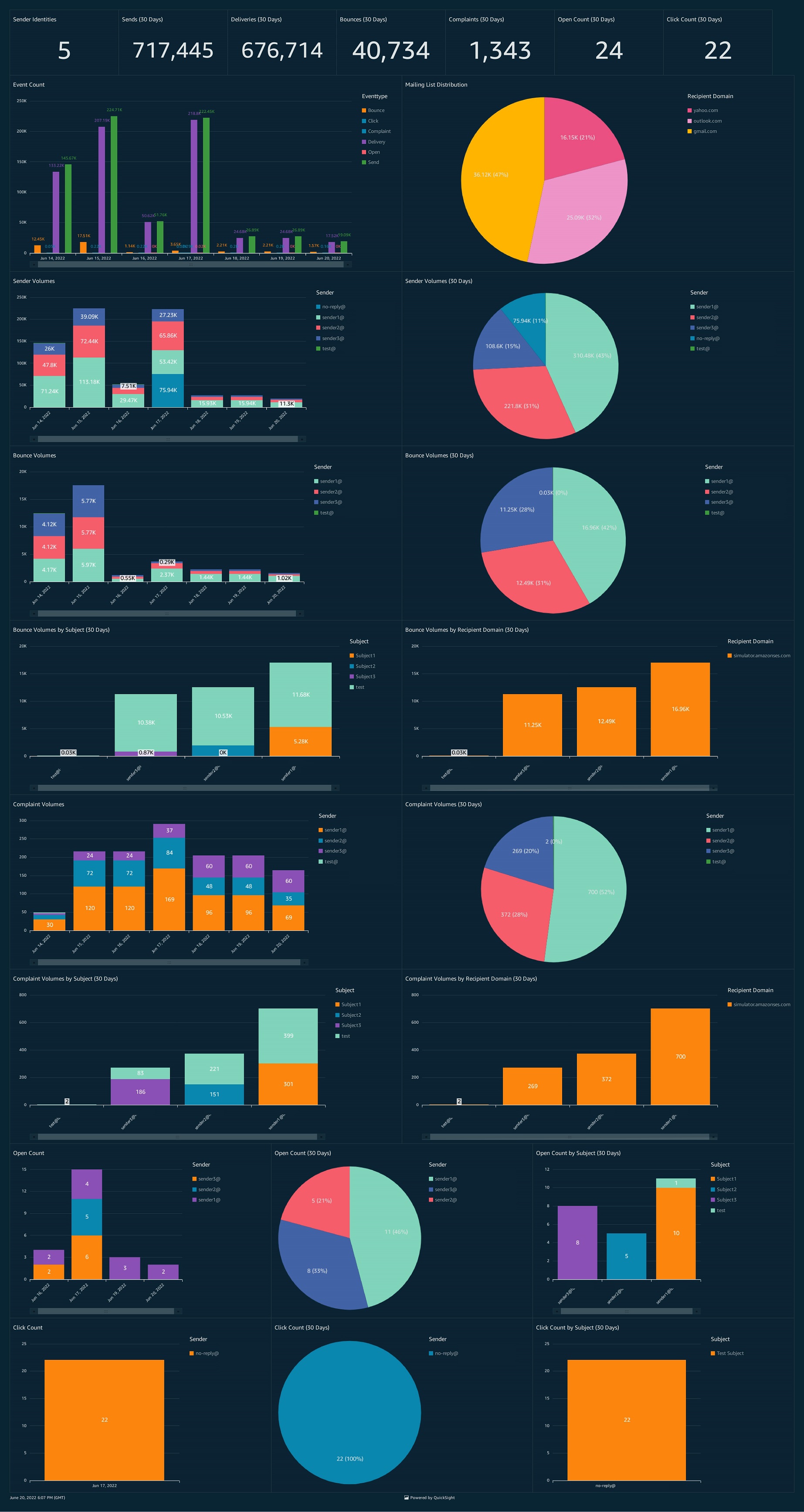
Amazon FinTech deals with petabytes of data and had built up a repository of 10,000 reports used by 2,500 employees across Amazon. Collaborating with the QuickSight team, they consolidated their reports to reduce redundancy and focus on what their finance customers needed. Amazon FinTech built 450 canned and over 1,800 ad hoc reports in QuickSight, developing a reusable solution with the QuickSight API. As shown in the following figure, on average per month, Amazon FinTech has over 1,300 unique QuickSight users run almost 2,500 unique QuickSight reports, with more than 4,600 total runs.

Amazon FinTech has been able to scale to meet customer requirements using QuickSight.

“AWS services come along with scalability. The whole point of migrating to AWS is that we do not need to think about scaling our infrastructure, and we can focus on the functional part of it,” says Barman.

QuickSight is cloud based, fully managed, and serverless, meaning you don’t have to build your own infrastructure to handle peak usage. It auto scales across tens of thousands of users who work independently and simultaneously.

As of May 2022, more than 2,500 Amazon Finance employees are using QuickSight for financial and operational reporting and to prepare Amazon’s tax statements.

“The advantage of Amazon QuickSight is that it empowers nontechnical users, including accountants and tax and financial analysts. It gives them more capability to run their reporting and build their own analyses,” says Keith Weiss, principal program manager at Amazon FinTech. According to Weiss, “QuickSight has much richer data visualization than competing BI tools.”

QuickSight is constantly innovating for customers, adding new features, and recently released the AI/ML service Amazon QuickSight Q, which lets users ask questions in natural language and receive accurate answers with relevant visualizations to help gain insights from the underlying data. Barman, Weiss, and the rest of the Amazon FinTech team are excited to implement Q in the near future.

By switching to QuickSight, which uses pay-as-you-go pricing, Amazon FinTech saved 40% without sacrificing the security, governance, and compliance requirements their account needed to comply with internal and external auditors. The AWS pricing structure makes QuickSight much more cost-effective than other BI tools on the market.

Overall, Amazon FinTech saw the following benefits:

  • Performance improvements – Latency of consumer-facing reports was reduced by 30%
  • Cost reduction – FinTech reduced licensing, database, and support costs by over 40%, and with the AWS pay-as-you-go model, it’s much more cost-effective to be on QuickSight
  • Controllership – FinTech reports are global, and controlled accessibility to reporting data is a key aspect to ensure only relevant data is visible to specific teams
  • Improved governance – QuickSight APIs to track and promote changes within different environments reduced manual overhead and improved change trackability

Seamless and reliable

At the end of each month, Amazon FinTech teams must close books in 5 days, and since implementing QuickSight for this purpose, Barman says that “reports have run seamlessly, and there have been no critical situations.”

Amazon FinTech’s account on QuickSight is now the source of truth for Amazon’s financial reporting, including tax filings and preparing financial statements. It enables Amazon’s own finance team to close its books and file taxes at the unparalleled scale at which Amazon operates, with all its complexity. Most importantly, despite initial skepticism, according to Weiss, “Our finance users love it.”

Learn more about Amazon QuickSight and get started diving deeper into your data today!


About the authors

Chitradeep Barman is a Sr. Technical Program Manager at Amazon Finance Technology (FinTech). He led the Amazon wide migration of BI reporting from Oracle BI (OBIEE) to AWS QuickSight. Chitradeep started his career as a data engineer and over time grew as a data architect. Before joining Amazon, he lead the design and implementation to launch the BI analytics and reporting platform for Cisco Capital (a fully owned subsidiary of Cisco Systems).

Yaniv Ackerman is a senior software development manager in Fintech org. He has over 20 years of experience building business critical, scalable and high-performance software. Yaniv’s team build data lakes, analytics and automation solutions for financial usage.

Amazon DevOps Guru increases Operational Efficiency for 605

Post Syndicated from Mohit Gadkari original https://aws.amazon.com/blogs/devops/amazon-devops-guru-increases-operational-efficiency-for-605/

605 is an independent TV measurement firm that offers advertising and content measurement, full-funnel attribution, media planning, optimization, and analytical solutions, all on top of their multi-source viewership data set covering over 21 million U.S. households. 605 has built their technology solutions on AWS with dozens of accounts and tens of thousands of resources to monitor.

As 605 continues to innovate and build new solutions, the size and complexity of their AWS deployment has also grown proportionally. Over time, managing their deployment has become an operational challenge for their current team. 605 has deployed different application performance monitoring (APM) tools and notification systems to help their observability staff scale and support their growing cloud environment. However, 605 realized that their continued growth on the cloud would necessitate either increasing their observability staff or assuming some risk of potential application performance issues or even outages.

Amazon DevOps Guru allowed 605 to find a third path forward. Rather than accepting the trade-off of hiring more staff or assuming more risk, 605 discovered that DevOps Guru provides an increase in operational efficiency using their existing staff resources by applying artificial intelligence (AI) to supplement their existing APM and notification platform. Layering DevOps Guru into their DevOps environment , 605 realized a 4-fold decrease in the number of alerts and notifications that proved to be false positives. In fact, 605 went from an environment where 76.2% of their alerts and notifications were false positives, to one with only 18.9% false positives simply by adding Amazon DevOps Guru. In the end, 605 can more effectively and efficiently manage their environment with existing resources and actually freeing-up DevOps brainpower to work on more strategically important initiatives than application management.

“Amazon DevOps Guru has provided insights that help us focus our infrastructure roadmap. Our current SIEM tools require building out alerting ahead of time, while DevOps Guru is constantly evolving, which prevents becoming stagnant in our monitoring. Reducing the risk of false positive alerts has saved countless engineering hours.”

Jared Williams, VP of Infrastructure and Architecture, 605

605 without DevOps Guru had their Amazon CloudWatch and Amazon Elastic Container Service for Kubernetes ( Amazon EKS) configured with different application performance monitoring and notification systems. They saw only 23.8 % legitimate alerts and notifications, where as with the integration with DevOps Guru the legitimate alerts and notifications went up to 81% for a 6-month time period.
605 are monitoring over 13+ AWS Accounts, 20+ Amazon EKS Clusters, 500+ Pods ,15000+ EC2 Instances, 500+ S3 Buckets and 55+ Application Load Balancers with DevOps Guru

605 without DevOps Guru had their Amazon CloudWatch and Amazon Elastic Container Service for Kubernetes ( Amazon EKS) configured with different application performance monitoring and notification systems. They saw only 23.8 % legitimate alerts and notifications, where as with the integration with DevOps Guru the legitimate alerts and notifications went up to 81% for a 6-month time period.

Figure 1. 605 are monitoring over 13+ AWS Accounts, 20+ Amazon EKS Clusters, 500+ Pods ,15000+ EC2 Instances, 500+ S3 Buckets and 55+ Application Load Balancers with DevOps Guru.

Amazon DevOps Guru is a service powered by applying artificial intelligence (AI) that’s designed to make it easy to improve an application’s operational performance and availability. DevOps Guru helps detect behaviors that deviate from normal operating patterns so that you can identify operational issues long before they impact your applications. DevOps Guru utilizes ML models informed by years of Amazon.com and AWS operational excellence to identify anomalous application behavior (for example, increased latency, error rates, resource constraints, and others). Furthermore, it helps surface critical issues that could cause potential outages or service disruptions. When DevOps Guru identifies a critical issue, it automatically sends an alert and provides a summary of related anomalies, the likely root cause, and context for when and where the issue occurred. When possible, DevOps Guru also helps provide recommendations regarding how to remediate the issue. DevOps Guru ingests operational data from your AWS applications and provides a single dashboard to visualize issues in your operational data. DevOps Guru can be enabled for all of the resources in your AWS account, resources in your AWS CloudFormation Stacks, or resources grouped together by AWS Tags, with no manual setup or ML expertise required.

The value of DevOps Guru for 605 goes beyond providing operational efficiency and avoiding the choice of adding DevOps resources or assuming more risk. DevOps Guru also discovered issues with application performance that their existing solutions weren’t trained to inspect.

This new data allowed 605 to avoid a potential problem that they didn’t otherwise know would occur. As DevOps Guru doesn’t require any set-up beyond enabling the service and choosing resources to monitor (it’s a managed service), the service can surface issues without any prior configuration.

In the end, the value of DevOps Guru for 605 surfaces in three ways. First, it increases operational efficiency by allowing their existing DevOps team to more effectively manage its AWS applications and resources, as well as the room to grow along with their business needs. Second, DevOps Guru reduces operational fatigue and allows their DevOps teams to focus on more strategic issues by significantly reducing false positives. Lastly, DevOps Guru can find operational issues to which existing APM tools may not be configured or able to detect.

Start monitoring your AWS applications with AWS DevOps Guru today using this link

About the authors:

Mohit Gadkari

Mohit Gadkari is a Solutions Architect at Amazon Web Services (AWS) supporting SMB customers. He has been professionally using AWS since 2015 specializing in DevOps and Cloud Security and currently he is using this experience to help customers navigate the cloud.

Pauly Longani

Pauly is an Enterprise Support Lead at AWS, USA. He is a customer advocate and supports his customers in their cloud journey. He is passionate about the cloud and how it can be leveraged to overcome challenges across industry verticals.

Jared Williams

Jared, VP of Infrastructure and Architecture at 605, is in his 15th year managing or working on teams with DevOps type focuses. He has been involved with AWS since 2009. He manages the multi-team DevOps department at 605 where he has been for more than three years. Jared also co-founded a 24,000+ person DevOps community.

Easily protect your AWS CDK-defined infrastructure with AWS WAFv2

Post Syndicated from Ramon Lopez Narvaez original https://aws.amazon.com/blogs/devops/easily-protect-your-aws-cdk-defined-infrastructure-with-aws-wafv2/

Security is a shared responsibility between AWS and the customer. When we use infrastructure as code (IaC) we want to describe workloads wholistically, and that includes the configuration of firewalls alongside the entrypoints to web applications. As we evolve the infrastructure that our application is built upon, we can adjust firewall rules in the same place.

In this post, you’ll learn how you can easily add a layer of protection to your web application that is defined in AWS Cloud Development Kit (AWS CDK) and built using Amazon CloudFront, Amazon API Gateway, Application Load Balancer, or AWS AppSync.

To accomplish this, we’ll use AWS WAFv2. Although it’s usually complex to write your own firewall rules, we can simply use AWS Managed Rules. No tedious setup required!

What is AWS WAFv2?

AWS WAFv2 is a managed web application firewall. It can be natively enabled on CloudFront, API Gateway, Application Load Balancer, or AWS AppSync and is deployed alongside these services. AWS services terminate the TCP/TLS connection, process incoming HTTP requests, and then pass the request to AWS WAF for inspection and filtering.

For example, you can use AWS WAFv2 to protect against attacks, such as cross-site request forgery (CSRF), cross-site scripting (XSS), and SQL injection (SQLi) among other threats in the OWASP Top 10.

AWS Managed Rules for AWS WAF is a set of AWS WAF rules curated and maintained by the AWS Threat Research Team that provides protection against common application vulnerabilities or other unwanted traffic, without having to write your own rules.

Prerequisites

For this walkthrough, you should have the following prerequisites:

  • An AWS account
  • An application fronted by one or more of the following services: Amazon Cloudfront, Amazon API Gateway, Application Load Balancer or AWS AppSync. From here on these are called ‘entrypoint’.
  • At least the above mentioned ‘entrypoint’ defined in AWS CDK.

Solution overview

When AWS WAF is applied to Amazon CloudFront, Amazon API Gateway, Application Load Balancer, or AWS AppSync, it inspects and filters requests before they’re forwarded to your compute infrastructure.

Figure 1. AWS WAFv2 can protect endpoints built by Amazon CloudFront, Amazon API Gateway, Application Load Balancer and AWS AppSync

Given that you have an existing web application defined in AWS CDK, we want to add a WAFv2 web ACL to its entrypoint. Instead of writing our own firewall rules to inspect and filter requests, we want to leverage an AWS Managed Rules rule group. Simultaneously, we must be able to disable or reconfigure some of the rules in the case that they cause undesirable behavior in the application.

A good first rule group to use is the core rule set (CRS) managed rule group, also named AWSManagedRulesCommonRuleSet. It contains rules that are generally applicable to web applications and provides protection against exploitation of various vulnerabilities, such as the ones described in the OWASP Top 10. You can later add more managed rule groups or write your own rules, which are specific to your application (e.g., for Windows, Linux, or WordPress).

Define the AWS WAFv2 web ACL

First, let’s give the AWS WAF module a nicely readable name:

import { aws_wafv2 as wafv2 } from 'aws-cdk-lib';

Then, we define the AWS WAFv2 web ACL in AWS CDK:

const cfnWebACL = new wafv2.CfnWebACL(this,'MyCDKWebAcl'
      defaultAction: {
        allow: {}
      },
      scope: 'REGIONAL',
      visibilityConfig: {
        cloudWatchMetricsEnabled: true,
        metricName:'MetricForWebACLCDK',
        sampledRequestsEnabled: true,
      },
      name:‘MyCDKWebAcl’,
      rules: [{
        name: 'CRSRule',
        priority: 0,
        statement: {
          managedRuleGroupStatement: {
            name:'AWSManagedRulesCommonRuleSet',
            vendorName:'AWS'
          }
        },
        visibilityConfig: {
          cloudWatchMetricsEnabled: true,
          metricName:'MetricForWebACLCDK-CRS',
          sampledRequestsEnabled: true,
        },
        overrideAction: {
          none: {}
        },
      }]
    });

The highlighted line references the CRS managed rule group as one Rule in the list. You could add more Rule elements, either referencing the managed rule groups or custom rules.

Note the scope attribute. If you want to attach this web ACL to an API Gateway, AWS AppSync API, or Application Load Balancer, then it will be REGIONAL. If you want to attach it to a CloudFront distribution, then make sure that your AWS WAFv2 web ACL is defined in the US East (N. Virginia) Region and the scope is CLOUDFRONT.

Attach the AWS WAFv2 web ACL to an Application Load Balancer, AWS AppSync API, or API Gateway

Now that we have a web ACL defined, we must attach it to a resource. This works exactly the same across API Gateway API’s, an AWS AppSync API, or an Application Load Balancer. We must create a CfnWebACLAssociation and point it to the previously created web ACL and the resource to protect:

const cfnWebACLAssociation = new wafv2.CfnWebACLAssociation(this,'MyCDKWebACLAssociation', {
      resourceArn:<ARN of resource to protect>,
      webAclArn:cfnWebACL.attrArn,
    });

Amazon Resource Names (ARNs) uniquely identify AWS resources. The highlighted line shows how AWS CDK lets you get the ARN of the previously defined CfnWebAcl.

Depending on what type of service you’re using, jump to one of the three following sections to learn how to retrieve the resourceArn of API Gateway, AWS AppSync, or Application Load Balancers.

Retrieving ARN for AWS AppSync API’s

To retrieve the ARN of an AWS AppSync API, call the .arn property:

const api = new appsync.GraphqlApi(…)
const cfnWebACLAssociation = new wafv2.CfnWebACLAssociation(this,'MyCDKWebACLAssociation', {
      resourceArn:api.arn,
      webAclArn: cfnWebACL.attrArn,
    });

Retrieving ARN for Amazon API Gateway REST API’s

In this case, we must specify which stage of the REST API we want to protect with the web ACL. Then, we reference the ARN of the stage:

const api = new apigateway.RestApi(…)
const deployment = new apigateway.Deployment(…)
const stage = apigateway.Stage(…)
const cfnWebACLAssociation = new wafv2.CfnWebACLAssociation(this,'MyCDKWebACLAssociation', {
      resourceArn:stage.stageArn,
      webAclArn: cfnWebACL.attrArn,
    });

Retrieving ARN for Application Load Balancers

If you’re dealing with an Application Load Balancer, then this is how you can retrieve its ARN:

const lb = new elbv2.ApplicationLoadBalancer(…)

const cfnWebACLAssociation = new wafv2.CfnWebACLAssociation(this,'MyCDKWebACLAssociation', {
      resourceArn:lb.loadBalancerArn,
      webAclArn: cfnWebACL.attrArn,
    });

Attach the AWS WAFv2 web ACL to a CloudFront distribution

Attaching a web ACL to CloudFront follows a different approach. Instead of defining a cfnWebACLAssociation, we reference the web ACL inside of the Distribution definition:

const distribution = new cloudfront.Distribution(this,'distro', {
      defaultBehavior: {
        origin: new origins.S3Origin(s3Bucket)
      },
     webAclId:cfnWebACL.attrArn
    });

Note that even though the property is called webAclId, because we’re using AWS WAFv2, we must supply the ARN of the web ACL.

Exclude rules from the web ACL

Lastly, let’s understand how we can customize the web ACL further. If a rule of the managed rule group causes undesired behavior in the application, then we can exclude it from the webACL. Assume that we want to exclude the SizeRestrictions_BODY rule, which limits the request body size to 8 KB.

Go back to the definition of the web ACL, and add the highlighted lines:

const cfnWebACL = new wafv2.CfnWebACL(this, 'MyCDKWebAcl', {
      defaultAction: {
        allow: {}
      },
      scope:'REGIONAL',
      visibilityConfig: {
        cloudWatchMetricsEnabled: true,
        metricName:'MetricForWebACLCDK',
        sampledRequestsEnabled: true,
      },
      name:'MyCDKWebAcl',
      rules: [{
        name:'CRSRule',
        priority: 0,
        statement: {
          managedRuleGroupStatement: {
            name: 'AWSManagedRulesCommonRuleSet',
            vendorName: 'AWS',
            excludedRules: [{
             ‘SizeRestrictions_BODY’ }]
          }
        },
        visibilityConfig: {
          cloudWatchMetricsEnabled: true,
          metricName:'MetricForWebACLCDK-CRS',
          sampledRequestsEnabled: true,
        },
        overrideAction: {
          none: {}
        },
      }]

    });

Other customizations you can do include pinning the version of the rule group and narrowing the scope of the request that the rule evaluates, using Scope-down statements.

Conclusion

In this post, you’ve seen how an AWS WAFv2 web ACL can be added to your existing infrastructure defined in AWS CDK. By using Managed Rules, your application benefits from a layer of protection that is curated and maintained by AWS security experts.

As a next step, you can learn how to include AWS WAFv2 metrics from Amazon CloudWatch into your application dashboards. This will give you perspective on how your web application is performing in conjunction with the AWS WAFv2 web ACL.

To learn more about AWS WAFv2 and how to manage web ACL’s, check out the official developer guide.

About the author:

Ramon Lopez

Ramon is a Senior Solutions Architect at AWS, where he guides, educates, and empowers customers of all sizes and industries to build successful businesses in the AWS cloud. He also built web services for 150+ million Amazon Prime customers and led a team of software engineers in a fast-paced global environment. After being immersed in one of the largest micro-service environments, he is a believer in the DevOps mantra of “You build it, you run it”.

Diving Deep into EC2 Spot Instance Cost and Operational Practices

Post Syndicated from Sheila Busser original https://aws.amazon.com/blogs/compute/diving-deep-into-ec2-spot-instance-cost-and-operational-practices/

This blog post is written by, Sudhi Bhat, Senior Specialist SA, Flexible Compute.

Amazon EC2 Spot Instances are one of the popular choices among customers looking to cost optimize their workload running on AWS. Spot Instances let you take advantage of unused Amazon Elastic Compute Cloud (Amazon EC2) capacity in the AWS cloud and are available at up to a 90% discount compared to On-Demand EC2 instance prices. The key difference between On-Demand Instances and Spot Instances is that Spot Instances can be interrupted by Amazon EC2, with two minutes of notification, when Amazon EC2 needs the capacity back. Spot Instances are recommended for various stateless, fault-tolerant, or flexible applications, such as big data, containerized workloads, continuous integration/continuous development (CI/CD), web servers, high-performance computing (HPC), and test and development workloads.

Customers asked us for fast and easy ways to track and optimize usage for different services. In this post, we’ll focus on tools and techniques that can provide useful insights into the usages and behavior of workloads using Spot Instances, as well as how we can leverage those techniques for troubleshooting and cost tracking purposes.

Operational tools

Instance selection

One of the best practices while using Spot Instances is to be flexible about instance types, Regions, and Availability Zones, as this gives Spot a better cross-section of compute pools to select and allocate your desired capacity. AWS makes it easier to diversify your instance selection in Auto Scaling groups and EC2 Fleet through features like Attribute-Based Instance Type Selection, where you can select the instance requirements as a set of attributes like vCPU, memory, storage, etc. These requirements are translated into matching instance types automatically.

Instance Selection using Attribute Based Instance Selection feature available during Auto Scaling Group creation

Considering that AWS Cloud spans across 25+ Regions and 80+ Availability Zones, finding the optimal location (either a Region or Availability Zone) to fulfil Spot capacity needs without launching a Spot can be very handy. This is especially true when AWS customers have the flexibility to run their workloads across multiple Regions or Availability Zones. This functionality can be achieved with one of the newer features called Amazon EC2 Spot placement score. Spot placement score provides a list of Regions or Availability Zones, each scored from 1 to 10, based on factors such as the requested instance types, target capacity, historical and current Spot usage trends, and the time of the request. The score reflects the likelihood of success when provisioning Spot capacity, with a 10 meaning that the request is highly likely to succeed.

Spot Placement Score feature is available in EC2 Dashboard

If you wish to specifically select and match your instances to your workloads to leverage them, then refer to Spot Instance Advisor to determine Spot Instances that meet your computing requirements with their relative discounts and associated interruption rates. Spot Instance Advisor populates the frequency of interruption and average savings over On-Demand instances based on the last 30 days of historical data. However, note that the past interruption behavior doesn’t predict the future availability of these instances. Therefore, as a part of instance diversity, try to leverage as many instances as possible regardless of whether or not an instance has a high level of interruptions.

Spot Instance pricing history

Understanding the price history for a specific Amazon EC2 Spot Instance can be useful during instance selection. However, tracking these pricing changes can be complex. Since November 2017, AWS launched a new pricing model that simplified the Spot purchasing experience. The new model gives AWS Customers predictable prices that adjust slowly over days and weeks, as Spot Instance prices are now determined based on long-term trends in supply and demand for Spot Instance capacity. The current Spot Instance prices can be viewed on AWS website, and the Spot Instance pricing history can be viewed on the Amazon EC2 console or accessed via AWS Command Line Interface (AWS CLI). Customers can continue to access the Spot price history for the last 90 days, filtering by instance type, operating system, and Availability Zone to understand how the Spot pricing has changed.

Spot Pricing History is available in EC2 DashboardAccessing Pricing history via AWS CLI using describe-spot-price-history or Get-EC2SpotPriceHistory (AWS Tools for Windows PowerShell).

aws ec2 describe-spot-price-history --start-time 2018-05-06T07:08:09 --end-time 2018-05-06T08:08:09 --instance-types c4.2xlarge --availability-zone eu-west-1a --product-description "Linux/UNIX (Amazon VPC)“
{
    "SpotPriceHistory": [
        {
            "Timestamp": "2018-05-06T06:30:30.000Z",
            "AvailabilityZone": "eu-west-1a",
            "InstanceType": "c4.2xlarge",
            "ProductDescription": "Linux/UNIX (Amazon VPC)",
            "SpotPrice": "0.122300"
        }
    ]
}

Spot Instance data feed

EC2 offers a mechanism to describe Spot Instance usage and pricing by providing a data feed that can be subscribed to. Therefore, the data feed is sent to an Amazon Simple Storage Service (Amazon S3) bucket on an hourly basis. Learn more about setting up the Spot Data feed and configuring the S3 bucket options in the documentation. A sample data feed would look like the following:

Sample Spot Instance data feed dataThe above example provides more information about Spot Instance in use, like m4.large Instance being used at the time as specified by Timestamp and MyBidID=sir-11wsgc6k representing the request that generated this instance usage, Charge=0.045 USD indicating the discounted price charged compared to the MyMaxPrice, which was set to On-Demand cost. This information can be useful during troubleshooting, as you can refer to the information about Spot Instances even if that specific instance has been terminated. Moreover, you could choose to extend the use of this data for simple querying and visualization/analytics purposes using Amazon Athena.

Amazon EC2 Spot Instance Interruption dashboard

Spot Instance interruptions are an inherent part of the Spot Instance lifecycle. For example, it’s always possible that your Spot Instance might be interrupted depending on how many unused EC2 instances are available. Therefore, you must make sure that your application is prepared for a Spot Instance interruption.

There are several best practices regarding handling Spot interruptions as described in the blog “Best practices for handling EC2 Spot Instance interruptions. Tracking Spot Instance interruptions can be useful in some scenarios, such as evaluating your workload for the tolerance for interruptions of a specific instance type, or to simply learn more about frequency of interruptions in your test environment so that you can fine-tune your instance selection. In these scenarios, you can use the EC2 Spot interruption dashboard, which is an opensource sample reference solution for logging Spot Instance interruptions. Spot Instance interruptions can fluctuate dynamically based on overall Spot Instance availability and demand for On-Demand Instances. However, it is important to note that tracking interruptions may not always represent the true Spot experience. Therefore, it’s recommended that this solution be used for those situations where Spot Instance interruptions inform a specific outcome, as it doesn’t accurately reflect system health or availability. It’s recommended to use this solution in dev/test environments to provide an educated view of how to use Spot Instances in production systems.

Open Source Solution available in github called Spot Interruption Dashboard for tracking Spot Interruption termination notices.

Cost management tools

AWS Pricing Calculator

AWS Pricing Calculator is a free tool that lets you create cost estimates for workloads that you run on AWS Services, including EC2 and Spot Instances. This calculator can greatly assist in calculating the cost of compute instances and estimating the future costs so that customers can compare the cost savings to be achieved before they even launch a Spot Instance as part of their solution. The AWS Pricing Calculator advanced estimate path offers six pricing strategies for Amazon EC2 instances. The pricing models include On-Demand, Reserved, Savings Plans, and Spot Instances. The estimates generated can also be exported to a CSV or PDF file format for quick sharing and additional analysis of the proposed architecture spend.

AWS Pricing Calculator support different types of workloadsFor Spot Instances, the calculator shows the historical average discount percentage for the instance chosen, and lets you enter a percentage discount for creating forecasts. We recommend choosing an instance type that best represents your target compute, memory, and network requirements for running your workload and generating an approximate estimate.

AWS Pricing Calculator Supports different type of EC2 Purchasing options, including EC2 Spot instances

AWS Cost Management

One of the popular reporting tools offered by AWS is AWS Cost Explorer, which has an easy-to-use interface that lets you visualize, understand, and manage your AWS costs and usage over time, including Spot Instances. You can view data up to the last 12 months, and forecast the next three months. You can use Cost Explorer filtered by “Purchase Options” to see patterns in how much you spend on Spot Instances over time, and see trends that you can use to understand your costs. Furthermore, you can specify time ranges for the data, and view time data by day or by month. Moreover, you can leverage the Amazon EC2 Instance Usage reports to gain insights into your instance usage and patterns, along with information that you need to optimize the overall EC2 use.

AWS Cost Explores shows cost incurred in multiple different compute purchasing options

AWS Billing and Cost Management offers a way to organize your resource costs on your cost allocation report by leveraging cost allocation tags, so that it’s easier to categorize and track your AWS costs using cost allocation reports, which includes all of your AWS costs for each billing period. The report includes both tagged and untagged resources, so that you can clearly organize the charges for resources. For example, if you tag resources with an application name that is deployed on Spot Instances, you can track the total cost of that single application that runs on those resources. The AWS generated tags “createdBy” is a tag that AWS defines and applies to supported AWS resources for cost allocation purposes and if opted, this tag is applied to “Spot-instance-request” resource type whenever the RequestSpotInstances API is invoked. This can be a great way to track the Spot Instance creation activities in your billing reports.

Cost and Usage Reports

AWS Customers have access to raw cost and usage data through the AWS Cost and Usage (AWS CUR) reports. These reports contain the most comprehensive information about your AWS usage and costs. Financial teams need this data so that they have an overview of their monthly, quarterly, and yearly AWS spend. But this data is equally valuable for technical teams who need detailed resource-level granularity to understand which resources are contributing to the spend, and what parts of the system to optimize. If you’re using Spot Instances for your compute needs, then AWS CUR populates the Amazon EC2 Spot usage pricing/* columns and the product/* columns. With this data, you can calculate the past savings achieved with Spot through the AWS CUR. Note that this feature was enabled in July 2021 and the AWS CUR data for Spot Usage is available only since then. The Cloud Intelligence Dashboards provide prebuilt visualizations that can help you get a detailed view of your AWS usage and costs. You can learn more about deploying Cloud Intelligence Dashboards by referring to the detailed blog “Visualize and gain insight into you AWS cost and usage with Cloud Intelligence Dashboard and CUDOS using Amazon QuickSite”Compute summary can be viewed in Cloud Intelligent Dashboards

Conclusion

It’s always recommended to follow Spot Instance best practices while using Amazon EC2 Spot Instances for suitable workloads, so that you can have the best experience. In this post, we explored a few tools and techniques that can further guide you toward much deeper insights into your workloads that are using Spot Instances. This can assist you with understanding cost savings and help you with troubleshooting so that you can use Spot Instances more easily.

How Fresenius Medical Care aims to save dialysis patient lives using real-time predictive analytics on AWS

Post Syndicated from Kanti Singh original https://aws.amazon.com/blogs/big-data/how-fresenius-medical-care-aims-to-save-dialysis-patient-lives-using-real-time-predictive-analytics-on-aws/

This post is co-written by Kanti Singh, Director of Data & Analytics at Fresenius Medical Care.

Fresenius Medical Care is the world’s leading provider of kidney care products and services, and operates more than 2,600 dialysis centers in the US alone. The company provides comprehensive solutions for people living with chronic kidney disease and related conditions, with a mission to improve the quality of life of every patient, every day, by transforming healthcare through research, innovation, and compassion. Data analysis that leads to timely interventions is critical to this mission, and essential to reduce hospitalizations and prevent adverse events.

In this post, we walk you through the solution architecture, performance considerations, and how a research partnership with AWS around medical complexity led to an automated solution that helped deliver alerts for potential adverse events.

Why Fresenius Medical Care chose AWS

The Fresenius Medical Care technical team chose AWS as their preferred cloud platform for two key reasons.

First, we determined that AWS IoT Core was more mature than other solutions and would likely face fewer issues with deployment and certificates. As an organization, we wanted to go with a cloud platform that had a proven track record and established technical solutions and services in the IoT and data analytics space. This included Amazon Athena, which is an easy-to-use serverless service that you can use to run queries on data stored in Amazon Simple Storage Service (Amazon S3) for analysis.

Another factor that played a major role in our decision was the fact that AWS offered the largest set of serverless services for analytics than any other cloud provider. We ultimately determined that AWS innovations met the company’s current needs as well as positioned the company for the future as we worked to expand our predictive capabilities.

Solution overview

We needed to develop a near-real-time analytics solution that would collect dynamic dialysis machine data every 10 seconds during hemodialysis treatment in near-real time and personalize it to predict every 30 minutes if a patient is at a health risk for intradialytic hypotension (IDH) within the next 15–75 minutes. This solution needed to scale to all our dialysis centers nationwide, with each location sending 10 MBps of treatment data at peak times.

The complexities that needed to be managed in the solution included handling high throughput data, a low-latency time-sensitive solution of 10 seconds from data origination to reporting and notification, a highly available solution, and a cost-effective solution with on-demand scaling up or down based on data volume.

Fresenius Medical Care partnered with AWS on this mission and developed an architecture that met our technical and business requirements. Core components in the architecture included Amazon Kinesis Data Streams, Amazon Kinesis Data Analytics, and Amazon SageMaker. We chose Kinesis Data Streams and Kinesis Data Analytics primarily because they’re serverless and highly available (99.9%), offer very high throughput, and are easy to scale. We chose SageMaker due to its unique capability that allows ease of building, training, and running machine learning (ML) models at scale.

The following diagram illustrates the architecture.

The solution consists of the following key components:

  1. Data collection
  2. Data ingestion and aggregation
  3. Data lake storage
  4. ML Inference and operational analytics

Let’s discuss each stage in the workflow in more detail.

Data collection

Dialysis machines located in Fresenius Medical Care centers help patients in the treatment of end-stage renal disease by performing hemodialysis. The dialysis machines provide immediate access to all treatment and clinical trending data across the fleet of hemodialysis machines in all centers in the US.

These machines transmit a data payload every 10 seconds to Kafka brokers located in Fresenius Medical Care’s on-premises data center for use by several applications.

Data ingestion and aggregation

We use a Kinesis-Kafka connector hosted on self-managed Amazon Elastic Compute Cloud (Amazon EC2) instances to ingest data from a Kafka topic in near-real time into Kinesis Data Streams.

We use AWS Lambda to read the data points and filter the datasets accordingly to Kinesis Data Analytics. Upon reaching the batch size threshold, Lambda sends the data to Kinesis Data Analytics for instream analytics.

We chose Kinesis Data Analytics due to the ease-of-use it provides for SQL-based stream analytics. By using SQL with KDA (KDA Studio/Flink SQL), we can create dynamic features based on machine interval data arriving in real time. This data is joined with the patient demographic, historical clinical, treatment, and laboratory data (enriched with Amazon S3 data) to create the complete set of features required for a downstream ML model.

Data lake storage

Amazon Kinesis Data Firehose was the simplest way to consistently load streaming data to build a raw data lake in Amazon S3. Kinesis Data Firehose micro-batches data into 128 MB file sizes and delivers streaming data to Amazon S3.

Clinical datasets are required to enrich stream data sourced from on-premises data warehouses via AWS Glue Spark jobs on a nightly basis. The AWS Glue jobs extract patient demographic, historical clinical, treatment, and laboratory data from the data warehouse to Amazon S3 and transform machine data from JSON to Parquet format for better storage and retrieval costs in Amazon S3. AWS Glue also helps build the static features for the intradialytic hypotension (IDH) ML model, which are required for downstream ML inference.

ML Inference and Operational analytics

Lambda batches the stream data from Kinesis Data Analytics that has all the features required for IDH ML model inference.

SageMaker, a fully managed service, trains and deploys the IDH predictive model. The deployed ML model provides a SageMaker endpoint that is used by Lambda for ML inference.

Amazon OpenSearch Service helps store the IDH inference results it received from Lambda. The results are then used for visualization through Kibana, which displays a personalized health prediction dashboard visual for each patient undergoing treatment and is available in near-real time for the care team to provide intervention proactively.

Observability and traceability for failures

Because this solution offers the potential for life-saving interventions, it’s considered business critical. The following key measures are taken to proactively monitor the AWS jobs in Fresenius Medical Care’s VPC account:

  • For AWS Glue jobs that have failures and errors in Lambda functions, an immediate email and Amazon CloudWatch alert is sent to the Data Ops team for resolution.
  • CloudWatch alarms are also generated for Amazon OpenSearch Service whenever there are blocks on writes or the cluster is overloaded with shard capacity, CPU utilization, or other issues, as recommended by AWS.
  • Kinesis Data Analytics and Kinesis Data Streams generate data quality alerts on data rejections or empty results.
  • Data quality alerts are also generated whenever data quality rules on data points are mismatched. To check mismatched data, we use quality rule comparison and sanity checks between message payloads in the stream with data loaded in the data lake.

These systematic and automated monitoring and alerting mechanisms help our team stay one step ahead to ensure that systems are running smoothly and successfully, and any unforeseen problems can be resolved as quickly as possible before it causes any adverse impact on users of the system.

AWS partnership

After Fresenius Medical Care took advantage of the AWS Data Lab to create a working prototype within one week, expert Solutions Architects from AWS became trusted advisors, helping our team with prescriptive guidance from ideation to production. The AWS team helped with both solution-based and service-specific best practices, helped resolve key blockers in every phase from development through production, and performed architecture reviews to ensure the solution was robust and resilient to business needs.

Solution results

This solution allows Fresenius Medical Care to better personalize care to patients undergoing dialysis treatment with a proactive intervention by clinicians at the point of care that has the potential to save patient lives. The following are some of the key benefits due to this solution:

  • Cloud computing resources enable the development, analysis, and integration of real-time predictive IDH that can be easily and seamlessly scaled as needed to reach additional clinics.
  • The use of our tool may be particularly useful in institutions facing staff shortages and, possibly, during home dialysis. Additionally, it may provide insights on strategies to prevent and manage IDH.
  • The solution enables modern and innovative solutions that improve patient care by providing world-class research and data-driven insights.

This solution has been proven to scale to an acceptable performance level of 6,000 messages per second, translating to 19 MB/sec with 60,000/sec concurrent Lambda invocations. The ability to adapt by scaling up and down every component in the architecture with ease kept costs very low, which wouldn’t have been possible elsewhere.

Conclusion

Successful implementation of this solution led to a think big approach in modernizing several legacy data assets and has set Fresenius Medical Care on the path of building an enterprise unified data analytics platform on AWS using Amazon S3, AWS Glue, Amazon EMR, and AWS Lake Formation. The unified data analytics platform offers robust data security and data sharing for multi-tenants in various geographies across the US. Similar to Fresenius, you can accelerate time to market by using the right tool for the job, using the broad and deep variety of AWS analytic native services.


About the authors

Kanti Singh is a Director of Data & Analytics at Fresenius Medical Care, leading the big data platform, architecture, and the engineering team. She loves to explore new technologies and how to leverage them to solve complex business problems. In her free time, she loves traveling, dancing, and spending time with family.

Harsha Tadiparthi is a Specialist Principal Solutions Architect specialized in analytics at Amazon Web Services. He enjoys solving complex customer problems in databases and analytics, and delivering successful outcomes. Outside of work, he loves to spend time with his family, watch movies, and travel whenever possible.

Removing complexity to improve business performance: How Bridgewater Associates built a scalable, secure, Spark-based research service on AWS

Post Syndicated from Sergei Dubinin original https://aws.amazon.com/blogs/big-data/removing-complexity-to-improve-business-performance-how-bridgewater-associates-built-a-scalable-secure-spark-based-research-service-on-aws/

This is a guest post co-written by Sergei Dubinin, Oleksandr Ierenkov, Illia Popov and Joel Thompson, from Bridgewater.

Bridgewater’s core mission is to understand how the world works by analyzing the drivers of markets and turning that understanding into high-quality portfolios and investment advice for our clients. Within Bridgewater Technology, we strive to make our researchers as productive as possible at what they do best: building the fundamental understanding of global markets. This means eliminating the need to deal with underlying IT infrastructure, and focusing on building and improving their investment ideas.

In this post, we examine our proprietary service in four dimensions. We talk about our business challenges, how we met our high security bar, how we can scale to meet the demands of the business, and how we do all of this in a cost-effective manner.

Challenge

Our researchers’ demand for compute required to develop and test their investment logic is constantly growing. This consistent and aggressive growth in compute capacity was a driving force behind our initial decision to move to the public cloud.

Utilizing the scale of the AWS Cloud has allowed us to generate investment signals and views of the world that would have been impossible to do on premises. When we first moved this analytical workload to AWS, we built on Amazon Elastic Compute Cloud (Amazon EC2) along with other services such as Elastic Load Balancing, AWS Auto Scaling, and Amazon Simple Storage Service (Amazon S3) to provide core functionality. A short time later, we moved to the AWS Nitro System, completing jobs 20% faster—allowing our research teams to iterate more quickly on their investment ideas.

The next step in our evolution started 2 years ago when we adopted Apache Spark as the underlying compute engine for our investment logic execution service. This helped streamline our analytics pipeline, removing duplication and decoupling many of the plugins we were developing for our researchers. Rather than run Apache Spark ourselves, we chose Amazon EMR as a hosted Spark platform. However, we soon discovered that Amazon EMR on EC2 wasn’t a good fit for the way we wanted to use it. For example, we can’t predict when a researcher will submit a job, so to avoid having our researchers wait for a brand new EMR cluster to be created and bootstrapped, we used long-lived EMR clusters, which forced many different jobs to run on the same cluster. However, because a single EMR cluster can only exist in a single Availability Zone, our cluster was limited to only being able to launch instances in that Availability Zone. At the significant scale that we were operating at, individual Availability Zones started running out of our desired instance capacity to meet our needs. Although we could launch many different clusters across different Availability Zones, that would leave us handling job scheduling at a high level, which was the whole point of using Amazon EMR and Spark. Furthermore, to be as cost-efficient as possible, we wanted to continuously scale the number of nodes in the cluster based on demand, and as a result, we would churn through thousands of nodes a day. This constant churning of nodes caused job failures and additional operational overhead for our teams.

We brought these concerns to AWS, who took the lead in pushing these issues to resolution. AWS partnered closely with us to understand our use cases and the impact of job failures, and tirelessly worked with us to solve these challenges. Working with the Amazon EMR team, we narrowed down the problem to our aggressive scaling patterns, which the service could not handle at that time. Over the course of just a few months, the Amazon EMR team made several service improvements in the scaling mechanism to meet our needs and the needs of many other AWS customers.

While working closely with the Amazon EMR team on these issues, the AWS team informed us of the development of Amazon EMR on EKS, a managed service that would enable us to run Spark workloads on Amazon Elastic Kubernetes Service (Amazon EKS). Amazon EKS is a strategic platform for us across various business units at Bridgewater, and after doing a proof of concept of our workload using EMR on EKS, it became clear that this was a better fit for our use case and more aligned with our strategic direction. After migrating to EMR on EKS, we can now take advantage of capacity in multiple Availability Zones and improve our resiliency to EMR cluster issues or broader service events, while still meeting our high security bar.

Security

Another important aspect of our service is ensuring it maintains the appropriate security posture. Among other concerns, Bridgewater strictly compartmentalizes access to different investment ideas, and we must defend against the possibility of a malicious insider attempting to steal our intellectual property or otherwise harm Bridgewater. To balance the trade-offs between speed and security, we designed security controls to defend against potentially malicious jobs, while enabling our researchers to quickly iterate on their code. This is made more complicated by the design of Spark’s Kubernetes backend. The Spark driver, which in our case is running arbitrary and untrusted code, has to be given Kubernetes role-based access control (RBAC) permissions to create Kubernetes Pods. The ability to create Pods is very powerful and can lead to privilege escalation.

Our first layer of isolation is to run each job in its own Kubernetes namespace (and, therefore, in its own EMR on EKS virtual cluster). A namespace and virtual cluster are created when the job is ready to be submitted, and they’re deleted when that job is finished. This prevents one job from interfering directly with another job, but there are still other vectors to defend against. For example, Spark drivers should not be creating Pods with containers that run as root or source their images from unapproved repositories. We first investigated PodSecurityPolicies for this purpose. However, they couldn’t solve all of our use cases (such as restricting where container images can be pulled from), and they are currently being deprecated and will eventually be removed. Instead, we turned to Open Policy Agent (OPA) Gatekeeper, which provides a flexible approach for writing policies in code that can do more complex authorization decisions and allows us to implement our desired suite of controls. We also worked with the AWS Service Team to add further defense in depth, such as ensuring that all Pods created by EMR on EKS dropped all Linux capabilities, which we could then enforce with Gatekeeper.

The following diagram illustrates how we can maintain the required job separation within our research service.

Scaling

One of the largest motivations of our evolution to Spark on Amazon EMR and then on EMR on EKS was improving the efficiency of our resource utilization by aggressively scaling based on demand. Our fundamental cause-and-effect understanding of markets and economies is powered by our systematic, high-performance compute Spark grid. We run simulations at a constantly increasing scale and need an architecture that can scale up and meet our foreseeable business needs for the next several years.

Our platform runs two types of jobs: ad hoc interactive and scheduled batch. Each type of job brings its own scaling complexities, and both benefited from the evolution to EMR on EKS. Ad hoc jobs can be submitted at any time throughout business hours, and the simulation determines how much compute capacity is needed. For example, a particular job may need one EC2 instance or 100 EC2 instances. This can translate to hundreds of EC2 instances needing to be spun up or down within a few minutes. The scheduled batch jobs run periodically throughout the day with predetermined simulations and similarly translates to hundreds of EC2 instances spinning up or down. In total, scaling up and down by many hundreds of EC2 instances in a few minutes is common, and we needed a solution that could meet those business requirements.

For this specific problem, we needed a solution that was able to handle aggressive scaling events on the order of hundreds of EC2 instances per minute. Additionally, when operating at this scale, it’s important to both diversify instance types and spread jobs across Availability Zones. EMR on EKS empowers us to run fully-managed Spark jobs on an EKS cluster that spans multiple Availability Zones and provides the option to choose a heterogeneous set of instance types for Amazon EKS. Spanning a single EKS cluster across Availability Zones enables us to utilize compute capacity across the entire Region, thereby increasing instance diversity and availability for this workload. Because Spark jobs are running within containers on Amazon EKS, we can easily swap out instance types within the EKS cluster or run different instance types within the same cluster. As a result of these capabilities, we’re able to regularly scale our production service to approximately 1,600 EC2 instances totaling 25,000 cores at peak, running 3,000 jobs per day.

Finally, in late 2021, we conducted some scaling tests to see what the realistic limits of our service are. We are happy to share that we were able to scale our service to three times our normal daily size in terms of compute and simulations run. This exercise has validated that we will be able to meet the increase in business demand without committing additional engineering resources to do so.

Cost management

In addition to significantly increasing our ability to scale, we also were able to design the solution to be extremely cost effective. Prior to EMR on EKS, we had two options for Spark jobs: either self-managed on Amazon EC2 or using Amazon EMR on EC2. Self-managing on Amazon EC2 meant that we needed to manage the complexities of scheduling jobs on nodes, manage the Spark clusters themselves, and develop a separate application to provision and stop EC2 instances as Spark jobs ran to scale the workloads. Amazon EMR on EC2 provides a managed service to run Spark workloads on Amazon EC2. However, for customers like us who need to operate in multiple Availability Zones and already have a technology footprint on Kubernetes, EMR on EKS made more sense.

Moving to EMR on EKS enables us to scale dynamically as jobs are submitted, generating huge cost savings. Simulation capacity is right-sized within the range of a few minutes; something that is not possible with another solution. Additionally, our investment in Amazon EC2 Compute Savings Plans provides us with the savings and flexibility to meet our needs; we just need to specify how many compute hours we’re committed to in a particular Region and AWS handles the rest. You can read more about the cost benefits of EMR on EKS in Amazon EMR on Amazon EKS provides up to 61% lower costs and up to 68% performance improvement for Spark workloads.

The future

Although we’re currently meeting our key users’ needs, we have prioritized several improvements to our service for the future. First, we plan on replacing the Kubernetes Cluster Autoscaler with Karpenter. Given our aggressive and frequent compute scaling, we have found that some jobs can be unexpectedly stopped using the Cluster Autoscaler. We experience this about six times a day. We expect Karpenter will greatly diminish the occurrence of this failure mode. To learn more about Karpenter, check out Introducing Karpenter – An Open-Source High-Performance Kubernetes Cluster Autoscaler.

Second, we’re moving several complementary services that are currently running on EC2 to EKS. This will increase our ability to deploy meaningful improvements for our business and increase resiliency to service events.

Finally, we are making longer term efforts to improve our resiliency to regional service events. We are exploring broadening our operations to other AWS Regions, which would allow us to increase our service availability as well as maintain our burst capacity.

Conclusion

Working closely with AWS teams, we were able to develop a scalable, secure, and cost-optimized service on AWS that allows our researchers to generate larger and more complex investment ideas without worrying about IT infrastructure. Our service runs our Spark-based simulations across multiple Availability Zones at near-full utilization without having to worry about building or maintaining a scheduling platform. Finally, we are able to meet and surpass our security benchmarks by creating job separation using native AWS constructs at scale. This has given us tremendous confidence that our mission-critical data is safe in the AWS Cloud.

Through this close partnership with AWS, Bridgewater is poised to anticipate and meet the rigorous demands of our researchers for years to come; something that was not possible in our old data centers or with our prior architecture. Our President and CTO, Igor Tsyganskiy, recently spoke with AWS at length on this partnership. For the video of this discussion, check out Merging Business and Tech – Bridgewater’s Guide to Drive Agility.

Acknowledgements

  • Igor Tsyganskiy, President and Chief Technology Officer, Bridgewater
  • Aaron Linsky, Sr. Product Manager, Bridgewater
  • Gopinathan Kannan, Sr. Mgr. Engineering, Amazon Web Services
  • Vaibhav Sabharwal, Sr. Customer Solutions Manager, Amazon Web Services
  • Joseph Marques, Senior Principal Engineer, Amazon Web Services
  • David Brown, VP EC2, Amazon Web Services

About the authors

Sergei Dubinin is an Engineering Manager with Bridgewater. He is passionate about building big data processing systems that are suitable for a secure, stable, and performant use in production.

Oleksandr Ierenkov is a Solution Architect for EPAM Systems. He has focused on helping Bridgewater migrate in-house distributed systems to microservices on Kubernetes and various AWS-managed services with a focus on operational efficiency. Oleksandr is basically the same name as Alexander, only Ukrainian.

Anthony Pasquariello is a Senior Solutions Architect at AWS based in New York City. He specializes in modernization and security for our advanced enterprise customers. Anthony enjoys writing and speaking about all things cloud. He’s pursuing an MBA, and received his MS and BS in Electrical & Computer Engineering.

Illia Popov is a Tech Lead for EPAM Systems. Illia has been working with Bridgewater since 2018 and was active in planning and implementing the migration to EMR on EKS. He is excited to continue delivering value to Bridgewater by adapting managed services in close cooperation with AWS.

Peter Sideris is a Sr. Technical Account Manager at AWS. He works with some of our largest and most complex customers to ensure their success in the AWS Cloud. Peter enjoys his family, marine reef keeping, and volunteers his time to the Boy Scouts of America in several capacities.

Joel Thompson is an Architect at Bridgewater Associates, where he has worked in a variety of technology roles over the past 13 years, including building some of the earliest foundations of AWS adoption at Bridgewater. He is passionate about solving complicated problems to securely deliver value to the business. Outside of work, Joel is an avid skier, helped co-found the fwd:cloudsec cloud security conference, and enjoys traveling to spend time with friends and family.

Deploy and manage OpenAPI/Swagger RESTful APIs with the AWS Cloud Development Kit

Post Syndicated from Luke Popplewell original https://aws.amazon.com/blogs/devops/deploy-and-manage-openapi-swagger-restful-apis-with-the-aws-cloud-development-kit/

This post demonstrates how AWS Cloud Development Kit (AWS CDK) Infrastructure as Code (IaC) constructs and AWS serverless technology can be used to build and deploy a RESTful Application Programming Interface (API) defined in the OpenAPI specification. This post uses an example API that describes  Widget resources and demonstrates how to use an AWS CDK Pipeline to:

  • Deploy a RESTful API stage to Amazon API Gateway from an OpenAPI specification.
  • Build and deploy an AWS Lambda function that contains the API functionality.
  • Auto-generate API documentation and publish it to an Amazon Simple Storage Service (Amazon S3)-hosted website served by the Amazon CloudFront content delivery network (CDN) service. This provides technical and non-technical stakeholders with versioned, current, and accessible API documentation.
  • Auto-generate client libraries for invoking the API and deploy them to AWS CodeArtifact, which is a fully-managed artifact repository service. This allows API client development teams to integrate with different versions of the API in different environments.

The diagram shown in the following figure depicts the architecture of the AWS services and resources described in this post.

 The architecture described in this post consists of an AWS CodePipeline pipeline, provisioned using the AWS CDK, that deploys the Widget API to AWS Lambda and API Gateway. The pipeline then auto-generates the API’s documentation as a website served by CloudFront and deployed to S3. Finally, the pipeline auto-generates a client library for the API and deploys this to CodeArtifact.

Figure 1 – Architecture

The code that accompanies this post, written in Java, is available here.

Background

APIs must be understood by all stakeholders and parties within an enterprise including business areas, management, enterprise architecture, and other teams wishing to consume the API. Unfortunately, API definitions are often hidden in code and lack up-to-date documentation. Therefore, they remain inaccessible for the majority of the API’s stakeholders. Furthermore, it’s often challenging to determine what version of an API is present in different environments at any one time.

This post describes some solutions to these issues by demonstrating how to continuously deliver up-to-date and accessible API documentation, API client libraries, and API deployments.

AWS CDK

The AWS CDK is a software development framework for defining cloud IaC and is available in multiple languages including TypeScript, JavaScript, Python, Java, C#/.Net, and Go. The AWS CDK Developer Guide provides best practices for using the CDK.

This post uses the CDK to define IaC in Java which is synthesized to a cloud assembly. The cloud assembly includes one to many templates and assets that are deployed via an AWS CodePipeline pipeline. A unit of deployment in the CDK is called a Stack.

OpenAPI specification (formerly Swagger specification)

OpenAPI specifications describe the capabilities of an API and are both human and machine-readable. They consist of definitions of API components which include resources, endpoints, operation parameters, authentication methods, and contact information.

Project composition

The API project that accompanies this post consists of three directories:

  • app
  • api
  • cdk

app directory

This directory contains the code for the Lambda function which is invoked when the Widget API is invoked via API Gateway. The code has been developed in Java as an Apache Maven project.

The Quarkus framework has been used to define a WidgetResource class (see src/main/java/aws/sample/blog/cdkopenapi/app/WidgetResources.java ) that contains the methods that align with HTTP Methods of the Widget API.
api directory

The api directory contains the OpenAPI specification file ( openapi.yaml ). This file is used as the source for:

  • Defining the REST API using API Gateway’s support for OpenApi.
  • Auto-generating the API documentation.
  • Auto-generating the API client artifact.

The api directory also contains the following files:

  • openapi-generator-config.yaml : This file contains configuration settings for the OpenAPI Generator framework, which is described in the section CI/CD Pipeline.
  • maven-settings.xml: This file is used support the deployment of the generated SDKs or libraries (Apache Maven artifacts) for the API and is described in the CI/CD Pipeline section of this post.

This directory contains a sub directory called docker . The docker directory contains a Dockerfile which defines the commands for building a Docker image:

FROM ruby:2.6.5-alpine
 
RUN apk update \
 && apk upgrade --no-cache \
 && apk add --no-cache --repository http://dl-cdn.alpinelinux.org/alpine/v3.14/main/ nodejs=14.20.0-r0 npm \
 && apk add git \
 && apk add --no-cache build-base
 
# Install Widdershins node packages and ruby gem bundler 
RUN npm install -g widdershins \
 && gem install bundler 
 
# working directory
WORKDIR /openapi
 
# Clone and install the Slate framework
RUN git clone https://github.com/slatedocs/slate
RUN cd slate \
 && bundle install

The Docker image incorporates two open source projects, the NodeJS Widdershins library and the Ruby Slate-framework. These are used together to auto-generate the documentation for the API from the OpenAPI specification.  This Dockerfile is referenced and built by the  ApiStack class, which is described in the CDK Stacks section of this post.

cdk directory

This directory contains an Apache Maven Project developed in Java for provisioning the CDK stacks for the  Widget API.

Under the  src/main/java  folder, the package  aws.sample.blog.cdkopenapi.cdk  contains the files and classes that define the application’s CDK stacks and also the entry point (main method) for invoking the stacks from the CDK Toolkit CLI:

  • CdkApp.java: This file contains the  CdkApp class which provides the main method that is invoked from the AWS CDK Toolkit to build and deploy the  application stacks.
  • ApiStack.java: This file contains the   ApiStack class which defines the  OpenApiBlogAPI   stack and is described in the CDK Stacks section of this post.
  • PipelineStack.java: This file contains the   PipelineStack class which defines the OpenAPIBlogPipeline  stack and is described in the CDK Stacks section of this post.
  • ApiStackStage.java: This file contains the  ApiStackStage class which defines a CDK stage. As detailed in the CI/CD Pipeline section of this post, a DEV stage, containing the  OpenApiBlogAPI stack resources for a DEV environment, is deployed from the  OpenApiBlogPipeline pipeline.

CDK stacks

ApiStack

Note that the CDK bundling functionality is used at multiple points in the  ApiStack  class to produce CDK Assets. The post, Building, bundling, and deploying applications with the AWS CDK, provides more details regarding using CDK bundling mechanisms.

The  ApiStack  class defines multiple resources including:

  • Widget API Lambda function: This is bundled by the CDK in a Docker container using the Java 11 runtime image.
  • Widget  REST API on API Gateway: The REST API is created from an Inline API Definition which is passed as an S3 CDK Asset. This asset includes a reference to the  Widget API OpenAPI specification located under the  api folder (see  api/openapi.yaml ) and builds upon the SpecRestApi construct and API Gateway’s support for OpenApi.
  • API documentation Docker Image Asset: This is the Docker image that contains the open source frameworks (Widdershins and Slate) that are leveraged to generate the API documentation.
  • CDK Asset bundling functionality that leverages the API documentation Docker image to auto-generate documentation for the API.
  • An S3 Bucket for holding the API documentation website.
  • An origin access identity (OAI) which allows CloudFront to securely serve the S3 Bucket API documentation content.
  • A CloudFront distribution which provides CDN functionality for the S3 Bucket website.

Note that the  ApiStack class features the following code which is executed on the  Widget API Lambda construct:

CfnFunction apiCfnFunction = (CfnFunction)apiLambda.getNode().getDefaultChild();
apiCfnFunction.overrideLogicalId("APILambda");

The CDK, by default, auto-assigns an ID for each defined resource but in this case the generated ID is being overridden with “APILambda”. The reason for this is that inside of the  Widget API OpenAPI specification (see  api/openapi.yaml ), there is a reference to the Lambda function by name (“APILambda”) so that the function can be integrated as a proxy for each listed API path and method combination. The OpenAPI specification includes this name as a variable to derive the Amazon Resource Name (ARN) for the Lambda function:

uri:
	Fn::Sub: "arn:aws:apigateway:${AWS::Region}:lambda:path/2015-03-31/functions/${APILambda.Arn}/invocations"

PipelineStack

The  PipelineStack class defines a CDK CodePipline construct which is a higher level construct and pattern. Therefore, the construct doesn’t just map directly to a single CloudFormation resource, but provisions multiple resources to fulfil the requirements of the pattern. The post, CDK Pipelines: Continuous delivery for AWS CDK applications, provides more detail on creating pipelines with the CDK.

final CodePipeline pipeline = CodePipeline.Builder.create(this, "OpenAPIBlogPipeline")
.pipelineName("OpenAPIBlogPipeline")
.selfMutation(true)
      .dockerEnabledForSynth(true)
      .synth(synthStep)
      .build();

CI/CD pipeline

The diagram in the following figure shows the multiple CodePipeline stages and actions created by the CDK CodePipeline construct that is defined in the PipelineStack class.

The CI/CD pipeline’s stages include the Source stage, the Synth stage, the Update pipeline, the Assets stage, and the DEV stage.

Figure 2 – CI/CD Pipeline

The stages defined include the following:

  • Source stage: The pipeline is passed the source code contents from this stage.
  • Synth stage: This stage consists of a Synth Action that synthesizes the CloudFormation templates for the application’s CDK stacks and compiles and builds the project Lambda API function.
  • Update Pipeline stage: This stage checks the OpenAPIBlogPipeline stack and reinitiates the pipeline when changes to its definition have been deployed.
  • Assets stage: The application’s CDK stacks produce multiple file assets (for example, zipped Lambda code) which are published to Amazon S3. Docker image assets are published to a managed CDK framework Amazon Elastic Container Registry (Amazon ECR) repository.
  • DEV stage: The API’s CDK stack ( OpenApiBlogAPI ) is deployed to a hypothetical development environment in this stage. A post stage deployment action is also defined in this stage. Through the use of a CDK ShellStep construct, a Bash script is executed that deploys a generated client Java Archive (JAR) for the Widget API to CodeArtifact. The script employs the OpenAPI Generator project for this purpose:
CodeBuildStep codeArtifactStep = CodeBuildStep.Builder.create("CodeArtifactDeploy")
    .input(pipelineSource)
    .commands(Arrays.asList(
           	"echo $REPOSITORY_DOMAIN",
           	"echo $REPOSITORY_NAME",
           	"export CODEARTIFACT_TOKEN=`aws codeartifact get-authorization-token --domain $REPOSITORY_DOMAIN --query authorizationToken --output text`",
           	"export REPOSITORY_ENDPOINT=$(aws codeartifact get-repository-endpoint --domain $REPOSITORY_DOMAIN --repository $REPOSITORY_NAME --format maven | jq .repositoryEndpoint | sed 's/\\\"//g')",
           	"echo $REPOSITORY_ENDPOINT",
           	"cd api",
           	"wget -q https://repo1.maven.org/maven2/org/openapitools/openapi-generator-cli/5.4.0/openapi-generator-cli-5.4.0.jar -O openapi-generator-cli.jar",
     	          "cp ./maven-settings.xml /root/.m2/settings.xml",
        	          "java -jar openapi-generator-cli.jar batch openapi-generator-config.yaml",
                    "cd client",
                    "mvn --no-transfer-progress deploy -DaltDeploymentRepository=openapi--prod::default::$REPOSITORY_ENDPOINT"
))
      .rolePolicyStatements(Arrays.asList(codeArtifactStatement, codeArtifactStsStatement))
.env(new HashMap<String, String>() {{
      		put("REPOSITORY_DOMAIN", codeArtifactDomainName);
            	put("REPOSITORY_NAME", codeArtifactRepositoryName);
       }})
      .build();

Running the project

To run this project, you must install the AWS CLI v2, the AWS CDK Toolkit CLI, a Java/JDK 11 runtime, Apache Maven, Docker, and a Git client. Furthermore, the AWS CLI must be configured for a user who has administrator access to an AWS Account. This is required to bootstrap the CDK in your AWS account (if not already completed) and provision the required AWS resources.

To build and run the project, perform the following steps:

  1. Fork the OpenAPI blog project in GitHub.
  2. Open the AWS Console and create a connection to GitHub. Note the connection’s ARN.
  3. In the Console, navigate to AWS CodeArtifact and create a domain and repository.  Note the names used.
  4. From the command line, clone your forked project and change into the project’s directory:
git clone https://github.com/<your-repository-path>
cd <your-repository-path>
  1. Edit the CDK JSON file at  cdk/cdk.json  and enter the details:
"RepositoryString": "<your-github-repository-path>",
"RepositoryBranch": "<your-github-repository-branch-name>",
"CodestarConnectionArn": "<connection-arn>",
"CodeArtifactDomain": "<code-artifact-domain-name>",
"CodeArtifactRepository": "<code-artifact-repository-name>"

Please note that for setting configuration values in CDK applications, it is recommend to use environment variables or AWS Systems Manager parameters.

  1. Commit and push your changes back to your GitHub repository:
git push origin main
  1. Change into the  cdk directory and bootstrap the CDK in your AWS account if you haven’t already done so (enter “Y” when prompted):
cd cdk
cdk bootstrap
  1. Deploy the CDK pipeline stack (enter “Y” when prompted):
cdk deploy OpenAPIBlogPipeline

Once the stack deployment completes successfully, the pipeline  OpenAPIBlogPipeline will start running. This will build and deploy the API and its associated resources. If you open the Console and navigate to AWS CodePipeline, then you’ll see a pipeline in progress for the API.

Once the pipeline has completed executing, navigate to AWS CloudFormation to get the output values for the  DEV-OpenAPIBlog  stack deployment:

  1. Select the  DEV-OpenAPIBlog  stack entry and then select the Outputs column. Record the REST_URL value for the key that begins with   OpenAPIBlogRestAPIEndpoint .
  2. Record the CLOUDFRONT_URL value for the key  OpenAPIBlogCloudFrontURL .

The API ping method at https://<REST_URL>/ping can now be invoked using your browser or an API development tool like Postman. Other API other methods, as defined by the OpenApi specification, are also available for invocation (For example, GET https://<REST_URL>/widgets).

To view the generated API documentation, open a browser at https://< CLOUDFRONT_URL>.

The following figure shows the API documentation website that has been auto-generated from the API’s OpenAPI specification. The documentation includes code snippets for using the API from multiple programming languages.

The API’s auto-generated documentation website provides descriptions of the API’s methods and resources as well as code snippets in multiple languages including JavaScript, Python, and Java.

Figure 3 – Auto-generated API documentation

To view the generated API client code artifact, open the Console and navigate to AWS CodeArtifact. The following figure shows the generated API client artifact that has been published to CodeArtifact.

The CodeArtifact service user interface in the Console shows the different versions of the API’s auto-generated client libraries.

Figure 4 – API client artifact in CodeArtifact

Cleaning up

  1. From the command change to the  cdk directory and remove the API stack in the DEV stage (enter “Y” when prompted):
cd cdk
cdk destroy OpenAPIBlogPipeline/DEV/OpenAPIBlogAPI
  1. Once this has completed, delete the pipeline stack:
cdk destroy OpenAPIBlogPipeline
  1. Delete the S3 bucket created to support pipeline operations. Open the Console and navigate to Amazon S3. Delete buckets with the prefix  openapiblogpipeline .

Conclusion

This post demonstrates the use of the AWS CDK to deploy a RESTful API defined by the OpenAPI/Swagger specification. Furthermore, this post describes how to use the AWS CDK to auto-generate API documentation, publish this documentation to a web site hosted on Amazon S3, auto-generate API client libraries or SDKs, and publish these artifacts to an Apache Maven repository hosted on CodeArtifact.

The solution described in this post can be improved by:

  • Building and pushing the API documentation Docker image to Amazon ECR, and then using this image in CodePipeline API pipelines.
  • Creating stages for different environments such as TEST, PREPROD, and PROD.
  • Adding integration testing actions to make sure that the API Deployment is working correctly.
  • Adding Manual approval actions for that are executed before deploying the API to PROD.
  • Using CodeBuild caching of artifacts including Docker images and libraries.

About the author:

Luke Popplewell

Luke Popplewell works primarily with federal entities in the Australian Government. In his role as an architect, Luke uses his knowledge and experience to help organisations reach their goals on the AWS cloud. Luke has a keen interest in serverless technology, modernization, DevOps and event-driven architectures.

How Fannie Mae built a data mesh architecture to enable self-service using Amazon Redshift data sharing

Post Syndicated from Kiran Ramineni original https://aws.amazon.com/blogs/big-data/how-fannie-mae-built-a-data-mesh-architecture-to-enable-self-service-using-amazon-redshift-data-sharing/

This post is co-written by Kiran Ramineni and Basava Hubli, from Fannie Mae.

Amazon Redshift data sharing enables instant, granular, and fast data access across Amazon Redshift clusters without the need to copy or move data around. Data sharing provides live access to data so that users always see the most up-to-date and transactionally consistent views of data across all consumers as data is updated in the producer. You can share live data securely with Amazon Redshift clusters in the same or different AWS accounts, and across Regions. Data sharing enables secure and governed collaboration within and across organizations as well as external parties.

In this post, we see how Fannie Mae implemented a data mesh architecture using Amazon Redshift cross-account data sharing to break down the silos in data warehouses across business units.

About Fannie Mae

Chartered by U.S. Congress in 1938, Fannie Mae advances equitable and sustainable access to homeownership and quality, affordable rental housing for millions of people across America. Fannie Mae enables the 30-year fixed-rate mortgage and drives responsible innovation to make homebuying and renting easier, fairer, and more accessible. We are focused on increasing operational agility and efficiency, accelerating the digital transformation of the company to deliver more value and reliable, modern platforms in support of the broader housing finance system.

Background

To fulfill the mission of facilitating equitable and sustainable access to homeownership and quality, affordable rental housing across America, Fannie Mae embraced a modern cloud-based architecture which leverages data to drive actionable insights and business decisions. As part of the modernization strategy, we embarked on a journey to migrate our legacy on-premises workloads to AWS cloud including managed services such as Amazon Redshift and Amazon S3. The modern data platform on AWS cloud serves as the central data store for analytics, research, and data science. In addition, this platform also serves for governance, regulatory and financial reports.

To address capacity, scalability and elasticity needs of a large data footprint of over 4PB, we decentralized and delegated ownership of the data stores and associated management functions to their respective business units. To enable decentralization, and efficient data access and management, we adopted a data mesh architecture.

Data mesh solution architecture

To enable a seamless access to data across accounts and business units, we looked at various options to build an architecture that is sustainable and scalable. The data mesh architecture allowed us to keep data of the respective business units in their own accounts, but yet enable a seamless access across the business unit accounts in a secure manner.  We reorganized the AWS account structure to have separate accounts for each of the business units wherein, business data and dependent applications were collocated in their respective AWS Accounts.

With this decentralized model, the business units independently manage the responsibility of hydration, curation and security of their data.  However, there is a critical need to enable seamless and efficient access to data across business units and an ability to govern the data usage. Amazon Redshift cross-account data sharing meets this need and enables us with business continuity.

To facilitate the self-serve capability on the data mesh, we built a web portal that allows for data discovery and ability to subscribe to data in the Amazon Redshift data warehouse and Amazon Simple Storage Service (Amazon S3) data lake (lake house). Once a consumer initiates a request on the web portal, an approval workflow is triggered with notification to the governance and business data owner. Upon successful completion of the request workflow, an automation process is triggered to grant access to the consumer, and a notification is sent to the consumer. Subsequently, the consumer is able to access the requested datasets. The workflow process of request, approval, and subsequent provisioning of access was automated using APIs and AWS Command Line Interface (AWS CLI) commands, and entire process is designed to complete within a few minutes.

With this new architecture using Amazon Redshift cross-account data sharing, we were able implement and benefit from the following key principles of a data mesh architecture that fit very well for our use case:

  • A data as a product approach
  • A federated model of data ownership
  • The ability for consumers to subscribe using self-service data access
  • Federated data governance with the ability to grant and revoke access

The following architecture diagram shows the high-level data mesh architecture we implemented at Fannie Mae. Data from each of the operational systems is collected and stored in individual lake houses and subscriptions are managed through a data mesh catalog in a centralized control plane account.

Fig 1. High level Data Mesh catalog architecture

Fig 1. High level Data Mesh catalog architecture

Control plane for data mesh

With a redesigned account structure, data are spread out across separate accounts for each business application area in S3 data lake or in Amazon Redshift cluster. We designed a hub and spoke point-to-point data distribution scheme with a centralized semantic search to enhance the data relevance. We use a centralized control plane account to store the catalog information, contract detail, approval workflow policies, and access management details for the data mesh. With a policy driven access paradigm, we enable fine-grained access management to the data, where we automated Data as a Service enablement with an optimized approach. It has three modules to store and manage catalog, contracts, and access management.

Data catalog

The data catalog provides the data glossary and catalog information, and helps fully satisfy governance and security standards. With AWS Glue crawlers, we create the catalog for the lake house in a centralized control plane account, and then we automate the sharing process in a secure manner. This enables a query-based framework to pinpoint the exact location of the data. The data catalog collects the runtime information about the datasets for indexing purposes, and provides runtime metrics for analytics on dataset usage and access patterns. The catalog also provides a mechanism to update the catalog through automation as new datasets become available.

Contract registry

The contract registry hosts the policy engine, and uses Amazon DynamoDB to store the registry policies. This has the details on entitlements to physical mapping of data, and workflows for the access management process. We also use this to store and maintain the registry of existing data contracts and enable audit capability to determine and monitor the access patterns. In addition, the contract registry serves as the store for state management functionality.

Access management automation

Controlling and managing access to the dataset is done through access management. This provides a just-in-time data access through IAM session policies using a persona-driven approach. The access management module also hosts event notification for data, such as frequency of access or number of reads, and we then harness this information for data access lifecycle management. This module plays a critical role in the state management and provides extensive logging and monitoring capabilities on the state of the data.

Process flow of data mesh using Amazon Redshift cross-account data sharing

The process flow starts with creating a catalog of all datasets available in the control plane account. Consumers can request access to the data through a web front-end catalog, and the approval process is triggered through the central control plane account. The following architecture diagram represents the high-level implementation of Amazon Redshift data sharing via the data mesh architecture. The steps of the process flow are as follows:

  1. All the data products, Amazon Redshift tables, and S3 buckets are registered in a centralized AWS Glue Data Catalog.
  2. Data scientists and LOB users can browse the Data Catalog to find the data products available across all lake houses in Fannie Mae.
  3. Business applications can consume the data in other lake houses by registering a consumer contract. For example, LOB1-Lakehouse can register the contract to utilize data from LOB3-Lakehouse.
  4. The contract is reviewed and approved by the data producer, which subsequently triggers a technical event via Amazon Simple Service Notification (Amazon SNS).
  5. The subscribing AWS Lambda function runs AWS CLI commands, ACLs, and IAM policies to set up Amazon Redshift data sharing and make data available for consumers.
  6. Consumers can access the subscribed Amazon Redshift cluster data using their own cluster.
Fig 2. Data Mesh architecture using Amazon Redshift data sharing

Fig 2. Data Mesh architecture using Amazon Redshift data sharing

The intention of this post is not to provide detailed steps for every aspect of creating the data mesh, but to provide a high-level overview of the architecture implemented, and how you can use various analytics services and third-party tools to create a scalable data mesh with Amazon Redshift and Amazon S3. If you want to try out creating this architecture, you can use these steps and automate the process using your tool of choice for the front-end user interface to enable users to subscribe to the dataset.

The steps we describe here are a simplified version of the actual implementation, so it doesn’t involve all the tools and accounts. To set up this scaled-down data mesh architecture, we demonstrate using cross-account data sharing using one control plane account and two consumer accounts. For this, you should have the following prerequisites:

  • Three AWS accounts, one for the producer <ProducerAWSAccount1>, and two consumer accounts: <ConsumerAWSAccount1> and <ConsumerAWSAccount2>
  • AWS permissions to provision Amazon Redshift and create an IAM role and policy
  • The required Amazon Redshift clusters: one for the producer in the producer AWS account, a cluster in ConsumerCluster1, and optionally a cluster in ConsumerCluster2
  • Two users in the producer account, and two users in consumer account 1:
    • ProducerClusterAdmin – The Amazon Redshift user with admin access on the producer cluster
    • ProducerCloudAdmin – The IAM user or role with rights to run authorize-data-share and deauthorize-data-share AWS CLI commands in the producer account
    • Consumer1ClusterAdmin – The Amazon Redshift user with admin access on the consumer cluster
    • Consumer1CloudAdmin – The IAM user or role with rights to run associate-data-share-consumer and disassociate-data-share-consumer AWS CLI commands in the consumer account

Implement the solution

On the Amazon Redshift console, log in to the producer cluster and run the following statements using the query editor:

CREATE DATASHARE ds;

ALTER DATASHARE ds ADD SCHEMA PUBLIC;
ALTER DATASHARE ds ADD TABLE table1;
ALTER DATASHARE ds ADD ALL TABLES IN SCHEMA sf_schema;

For sharing data across AWS accounts, you can use the following GRANT USAGE command. For authorizing the data share, typically it will be done by a manager or approver. In this case, we show how you can automate this process using the AWS CLI command authorize-data-share.

GRANT USAGE ON DATASHARE ds TO ACCOUNT <CONSUMER ACCOUNT>;

aws redshift authorize-data-share --data-share-arn <DATASHARE ARN> --consumer-identifier <CONSUMER ACCOUNT>

For the consumer to access the shared data from producer, an administrator on the consumer account needs to associate the data share with one or more clusters. This can be done using the Amazon Redshift console or AWS CLI commands. We provide the following AWS CLI command because this is how you can automate the process from the central control plane account:

aws redshift associate-data-share-consumer --no-associate-entire-account --data-share-arn <DATASHARE ARN> --consumer-arn <CONSUMER CLUSTER ARN>

/* Create Database in Consumer Account */
CREATE DATABASE ds_db FROM DATASHARE ds OF ACCOUNT <PRODUCER ACCOUNT> NAMESPACE <PRODUCER CLUSTER NAMESPACE>;

Optional:
CREATE EXTERNAL SCHEMA Schema_from_datashare FROM REDSHIFT DATABASE 'ds_db' SCHEMA 'public';

GRANT USAGE ON DATABASE ds_db TO user/group;

/* Optional:Grant usage on database to users or groups */
GRANT USAGE ON SCHEMA Schema_from_datashare TO GROUP Analyst_group;

To enable Amazon Redshift Spectrum cross-account access to AWS Glue and Amazon S3, and the IAM roles required, refer to How can I create Amazon Redshift Spectrum cross-account access to AWS Glue and Amazon S3.

Conclusion

Amazon Redshift data sharing provides a simple, seamless, and secure platform for sharing data in a domain-oriented distributed data mesh architecture. Fannie Mae deployed the Amazon Redshift data sharing capability across the data lake and data mesh platforms, which currently hosts over 4 petabytes worth of business data. The capability has been seamlessly integrated with their Just-In-Time (JIT) data provisioning framework enabling a single-click, persona-driven access to data. Further, Amazon Redshift data sharing coupled with Fannie Mae’s centralized, policy-driven data governance framework greatly simplified access to data in the lake ecosystem while fully conforming to the stringent data governance policies and standards. This demonstrates that Amazon Redshift users can create data share as product to distribute across many data domains.

In summary, Fannie Mae was able to successfully integrate the data sharing capability in their data ecosystem to bring efficiencies in data democratization and introduce a higher velocity, near real-time access to data across various business units. We encourage you to explore the data sharing feature of Amazon Redshift to build your own data mesh architecture and improve access to data for your business users.


About the authors

Kiran Ramineni is Fannie Mae’s Vice President Head of Single Family, Cloud, Data, ML/AI & Infrastructure Architecture, reporting to the CTO and Chief Architect. Kiran and team spear headed cloud scalable Enterprise Data Mesh (Data Lake) with support for Just-In-Time (JIT), and Zero Trust as it applies to Citizen Data Scientist and Citizen Data Engineers. In the past Kiran built/lead several internet scalable always-on platforms.

Basava Hubli is a Director & Lead Data/ML Architect at Enterprise Architecture. He oversees the Strategy and Architecture of Enterprise Data, Analytics and Data Science platforms at Fannie Mae. His primary focus is on Architecture Oversight and Delivery of Innovative technical capabilities that solve for critical Enterprise business needs. He leads a passionate and motivated team of architects who are driving the modernization and adoption of the Data, Analytics and ML platforms on Cloud. Under his leadership, Enterprise Architecture has successfully deployed several scalable, innovative platforms & capabilities that includes, a fully-governed Data Mesh which hosts peta-byte scale business data and a persona-driven, zero-trust based data access management framework which solves for the organization’s data democratization needs.

Rajesh Francis is a Senior Analytics Customer Experience Specialist at AWS. He specializes in Amazon Redshift and focuses on helping to drive AWS market and technical strategy for data warehousing and analytics. Rajesh works closely with large strategic customers to help them adopt our new services and features, develop long-term partnerships, and feed customer requirements back to our product development teams to guide the direction of our product offerings.

Kiran Sharma is a Senior Data Architect in AWS Professional Services. Kiran helps customers architecting, implementing and optimizing peta-byte scale Big Data Solutions on AWS.

How NerdWallet uses AWS and Apache Hudi to build a serverless, real-time analytics platform

Post Syndicated from Kevin Chun original https://aws.amazon.com/blogs/big-data/how-nerdwallet-uses-aws-and-apache-hudi-to-build-a-serverless-real-time-analytics-platform/

This is a guest post by Kevin Chun, Staff Software Engineer in Core Engineering at NerdWallet.

NerdWallet’s mission is to provide clarity for all of life’s financial decisions. This covers a diverse set of topics: from choosing the right credit card, to managing your spending, to finding the best personal loan, to refinancing your mortgage. As a result, NerdWallet offers powerful capabilities that span across numerous domains, such as credit monitoring and alerting, dashboards for tracking net worth and cash flow, machine learning (ML)-driven recommendations, and many more for millions of users.

To build a cohesive and performant experience for our users, we need to be able to use large volumes of varying user data sourced by multiple independent teams. This requires a strong data culture along with a set of data infrastructure and self-serve tooling that enables creativity and collaboration.

In this post, we outline a use case that demonstrates how NerdWallet is scaling its data ecosystem by building a serverless pipeline that enables streaming data from across the company. We iterated on two different architectures. We explain the challenges we ran into with the initial design and the benefits we achieved by using Apache Hudi and additional AWS services in the second design.

Problem statement

NerdWallet captures a sizable amount of spending data. This data is used to build helpful dashboards and actionable insights for users. The data is stored in an Amazon Aurora cluster. Even though the Aurora cluster works well as an Online Transaction Processing (OLTP) engine, it’s not suitable for large, complex Online Analytical Processing (OLAP) queries. As a result, we can’t expose direct database access to analysts and data engineers. The data owners have to solve requests with new data derivations on read replicas. As the data volume and the diversity of data consumers and requests grow, this process gets more difficult to maintain. In addition, data scientists mostly require data files access from an object store like Amazon Simple Storage Service (Amazon S3).

We decided to explore alternatives where all consumers can independently fulfill their own data requests safely and scalably using open-standard tooling and protocols. Drawing inspiration from the data mesh paradigm, we designed a data lake based on Amazon S3 that decouples data producers from consumers while providing a self-serve, security-compliant, and scalable set of tooling that is easy to provision.

Initial design

The following diagram illustrates the architecture of the initial design.

The design included the following key components:

  1. We chose AWS Data Migration Service (AWS DMS) because it’s a managed service that facilitates the movement of data from various data stores such as relational and NoSQL databases into Amazon S3. AWS DMS allows one-time migration and ongoing replication with change data capture (CDC) to keep the source and target data stores in sync.
  2. We chose Amazon S3 as the foundation for our data lake because of its scalability, durability, and flexibility. You can seamlessly increase storage from gigabytes to petabytes, paying only for what you use. It’s designed to provide 11 9s of durability. It supports structured, semi-structured, and unstructured data, and has native integration with a broad portfolio of AWS services.
  3. AWS Glue is a fully managed data integration service. AWS Glue makes it easier to categorize, clean, transform, and reliably transfer data between different data stores.
  4. Amazon Athena is a serverless interactive query engine that makes it easy to analyze data directly in Amazon S3 using standard SQL. Athena scales automatically—running queries in parallel—so results are fast, even with large datasets, high concurrency, and complex queries.

This architecture works fine with small testing datasets. However, the team quickly ran into complications with the production datasets at scale.

Challenges

The team encountered the following challenges:

  • Long batch processing time and complexed transformation logic – A single run of the Spark batch job took 2–3 hours to complete, and we ended up getting a fairly large AWS bill when testing against billions of records. The core problem was that we had to reconstruct the latest state and rewrite the entire set of records per partition for every job run, even if the incremental changes were a single record of the partition. When we scaled that to thousands of unique transactions per second, we quickly saw the degradation in transformation performance.
  • Increased complexity with a large number of clients – This workload contained millions of clients, and one common query pattern was to filter by single client ID. There were numerous optimizations that we were forced to tack on, such as predicate pushdowns, tuning the Parquet file size, using a bucketed partition scheme, and more. As more data owners adopted this architecture, we would have to customize each of these optimizations for their data models and consumer query patterns.
  • Limited extendibility for real-time use cases – This batch extract, transform, and load (ETL) architecture wasn’t going to scale to handle hourly updates of thousands of records upserts per second. In addition, it would be challenging for the data platform team to keep up with the diverse real-time analytical needs. Incremental queries, time-travel queries, improved latency, and so on would require heavy investment over a long period of time. Improving on this issue would open up possibilities like near-real-time ML inference and event-based alerting.

With all these limitations of the initial design, we decided to go all-in on a real incremental processing framework.

Solution

The following diagram illustrates our updated design. To support real-time use cases, we added Amazon Kinesis Data Streams, AWS Lambda, Amazon Kinesis Data Firehose and Amazon Simple Notification Service (Amazon SNS) into the architecture.

The updated components are as follows:

  1. Amazon Kinesis Data Streams is a serverless streaming data service that makes it easy to capture, process, and store data streams. We set up a Kinesis data stream as a target for AWS DMS. The data stream collects the CDC logs.
  2. We use a Lambda function to transform the CDC records. We apply schema validation and data enrichment at the record level in the Lambda function. The transformed results are published to a second Kinesis data stream for the data lake consumption and an Amazon SNS topic so that changes can be fanned out to various downstream systems.
  3. Downstream systems can subscribe to the Amazon SNS topic and take real-time actions (within seconds) based on the CDC logs. This can support use cases like anomaly detection and event-based alerting.
  4. To solve the problem of long batch processing time, we use Apache Hudi file format to store the data and perform streaming ETL using AWS Glue streaming jobs. Apache Hudi is an open-source transactional data lake framework that greatly simplifies incremental data processing and data pipeline development. Hudi allows you to build streaming data lakes with incremental data pipelines, with support for transactions, record-level updates, and deletes on data stored in data lakes. Hudi integrates well with various AWS analytics services such as AWS Glue, Amazon EMR, and Athena, which makes it a straightforward extension of our previous architecture. While Apache Hudi solves the record-level update and delete challenges, AWS Glue streaming jobs convert the long-running batch transformations into low-latency micro-batch transformations. We use the AWS Glue Connector for Apache Hudi to import the Apache Hudi dependencies in the AWS Glue streaming job and write transformed data to Amazon S3 continuously. Hudi does all the heavy lifting of record-level upserts, while we simply configure the writer and transform the data into Hudi Copy-on-Write table type. With Hudi on AWS Glue streaming jobs, we reduce the data freshness latency for our core datasets from hours to under 15 minutes.
  5. To solve the partition challenges for high cardinality UUIDs, we use the bucketing technique. Bucketing groups data based on specific columns together within a single partition. These columns are known as bucket keys. When you group related data together into a single bucket (a file within a partition), you significantly reduce the amount of data scanned by Athena, thereby improving query performance and reducing cost. Our existing queries are filtered on the user ID already, so we significantly improve the performance of our Athena usage without having to rewrite queries by using bucketed user IDs as the partition scheme. For example, the following code shows total spending per user in specific categories:
    SELECT ID, SUM(AMOUNT) SPENDING
    FROM "{{DATABASE}}"."{{TABLE}}"
    WHERE CATEGORY IN (
    'ENTERTAINMENT',
    'SOME_OTHER_CATEGORY')
    AND ID_BUCKET ='{{ID_BUCKET}}'
    GROUP BY ID;

  1. Our data scientist team can access the dataset and perform ML model training using Amazon SageMaker.
  2. We maintain a copy of the raw CDC logs in Amazon S3 via Amazon Kinesis Data Firehose.

Conclusion

In the end, we landed on a serverless stream processing architecture that can scale to thousands of writes per second within minutes of freshness on our data lakes. We’ve rolled out to our first high-volume team! At our current scale, the Hudi job is processing roughly 1.75 MiB per second per AWS Glue worker, which can automatically scale up and down (thanks to AWS Glue auto scaling). We’ve also observed an outstanding improvement of end-to-end freshness at less than 5 minutes due to Hudi’s incremental upserts vs. our first attempt.

With Hudi on Amazon S3, we’ve built a high-leverage foundation to personalize our users’ experiences. Teams that own data can now share their data across the organization with reliability and performance characteristics built into a cookie-cutter solution. This enables our data consumers to build more sophisticated signals to provide clarity for all of life’s financial decisions.

We hope that this post will inspire your organization to build a real-time analytics platform using serverless technologies to accelerate your business goals.


About the authors

Kevin Chun is a Staff Software Engineer in Core Engineering at NerdWallet. He builds data infrastructure and tooling to help NerdWallet provide clarity for all of life’s financial decisions.

Dylan Qu is a Specialist Solutions Architect focused on big data and analytics with Amazon Web Services. He helps customers architect and build highly scalable, performant, and secure cloud-based solutions on AWS.

Forwood Safety uses Amazon QuickSight Q to extend life-saving safety analytics to larger audiences

Post Syndicated from Faye Crompton original https://aws.amazon.com/blogs/big-data/forwood-safety-uses-amazon-quicksight-q-to-extend-life-saving-safety-analytics-to-larger-audiences/

This is a guest post by Faye Crompton from Forwood Safety. Forwood provides fatality prevention solutions to organizations across the globe.

At Forwood Safety, we have a laser focus on saving lives. Our solutions, which provide full content and proven methodology via verification tools and analytical capabilities, have one purpose: eliminating fatalities in the workplace. We recently realized an ambition to provide interactive, dynamic data visualization tools that enable our end users to access safety data in the field, regardless of their experience with analytics and data reporting.

In this post, I’ll talk about how Amazon QuickSight Q solved these challenges by giving users fast data insights through natural language querying capabilities.

Driving data insights with QuickSight

Forwood’s Critical Risk Management (CRM) solution provides organizations with globally benchmarked and comprehensive critical control checklists and verification controls that are proven to prevent fatalities in the workplace. CRM protects frontline workers from serious harm by helping change the culture of risk management for companies. In addition, our Forwood Analytical Self-Service Tool (FAST) enables our customers to use self-service reporting to get updated dashboards that display key safety and fatality prevention metrics.

For several years, we used AWS QuickSight to provide data visualization for our CRM and FAST reporting products, with great success. Most of our technology stack was already based on AWS, so we knew QuickSight would be easy to integrate. QuickSight is agnostic in terms of data sources and types, and it’s a very flexible tool. It’s also an open data technology, so it can accept most of the data sources that we throw at it. Most importantly, it ties in seamlessly with our own architecture and data pipelines in a way that our previous BI tools couldn’t. After we implemented QuickSight, we started using it to power both CRM and FAST, visualizing risk data and serving it back to our customers.

Using QuickSight Q to help site supervisors get answers quickly

Furthering our focus on innovation and usability; we identified a common challenge that we believed QuickSight could solve through our FAST application on behalf of our clients — we needed to make risk data more accessible for those of our clients who aren’t data analysts. We recognize that not everyone is an analyst. We also have mining industry customers who are not frequently accessing our applications via desktop. For example, mining site Supervisors and Operators working deep underground typically have access only via their mobile devices. For these users, it’s easier for them to ask the questions relevant to their specific use cases as needed at point of use, rather than filter and search through a dashboard to find the answers ahead of time.

QuickSight Q was the perfect solution to this challenge. QuickSight Q is a feature within QuickSight that uses machine learning to understand questions and how they relate to business data. The feature provides data insights and visualizations within seconds. With this capability, users can simply type in questions in natural language to access data insights about risk and compliance. Mining site workers, for example, can ask if the site is safe or if the right verification processes are in place. Health and safety teams and mining site supervisors can ask questions such as “Which sites should I verify today?” or “Which risk will be highest next week?” and receive a chart with the relevant data.

Making data more accessible to everyone

QuickSight Q gives our on-site customers near-real-time risk and compliance data from their mobile devices in a way they couldn’t before. With QuickSight Q, we can give our FAST users the opportunity to quickly visualize any fatality risks at their sites based on updated fatality prevention data. All users, not just analysts, can identify worksites that have a higher fatality risk because the data can show trends in non-compliance with safety standards. Our clients no longer have to look in a dashboard for the answers to their questions; those looking at a dashboard can go beyond the dashboard and ask deeper questions.

QuickSight Q solved one of our main BI challenges: how to make risk data more accessible to more people without extensive user training and technical understanding. Soon, we hope to use QuickSight Q as part of a multidimensional predictive dataset using deep learning models to deliver even more insights to our customers.

We look forward to extending our use of QuickSight. When we first started using it, it was strictly for analytics on our existing data. More recently, we started using API deployments for QuickSight. We have many different clients, and we use the API feature to maintain master versions of all 30+ standard reports, and then deploy those dashboards to as many clients as we need to via code. Previously, we saw QuickSight as a function of our analytics products; now we see it as a powerful and flexible toolkit of analytics features that our developers can build with.

Additionally, we look forward to relying on QuickSight Q to bring life-saving safety analytics to more people. QuickSight Q bridges the gap between the data a company has and the decisions that company needs to make, and that’s very powerful for our clients. Forwood Safety is driven to eradicate workplace fatalities, and by getting data to more people and making it easy to access, we can make our solutions more effective, saving more lives.


About the author

Faye Crompton is Head of Analytics, Safety Applications and Computer Vision at Forwood Safety. She leads work on analytics and safety products that reduce fatality risk in mining and other high-risk industries.

How to prepare your application to scale reliably with Amazon EC2

Post Syndicated from Sheila Busser original https://aws.amazon.com/blogs/compute/how-to-prepare-your-application-to-scale-reliably-with-amazon-ec2/

This blog post is written by, Gabriele Postorino, Senior Technical Account Manager, and Giorgio Bonfiglio, Principal Technical Account Manager

In this post, we’ll discuss how you can prepare for planned and unplanned scaling events with

Most of the challenges related to horizontal scaling can be mitigated by optimizing the architectural implementation and applying improvements in operational processes.

In the following sections, we’ll explore this in depth. Recommendations can be applied partially or fully – they come with different complexities, and each one will help you reduce the risk of facing insufficient capacity errors or scaling delays, as well as deliver enhancements in areas such as fault tolerance, elasticity, and cost optimization.

Architectural best practices

Instance capacity can be regarded as being divided into “pools” defined by AZ (such as us-east-1a), instance type (for example m5.xlarge), and tenancy. Combining the following two guidelines will widen the capacity pools available to scale out your fleets of instances. This will help you reduce costs, transparently recover from failures, and increase your application scalability.

Instance flexibility

Whether you’re migrating a new workload to the cloud, or tuning an existing workload, you’ll likely evaluate which compute configuration options are available and determine the right configuration for your application.

If your workload is already running on EC2 instances, you might already be aware of the instance type that it runs best on. Let’s say that your application is RAM intensive, and you found that r6i.4xlarge instances are best suited for it.

However, relying on a single instance type might result in artificially limiting your ability to scale compute resources for your workload when needed. It’s always a good idea to explore how your workload behaves when running on other instance types: you might find that your application can serve double the number of requests served by one r6i.4xlarge instance when using one r6i.8xlarge instance or four r6i.2xlarge instances.

Furthermore, there’s no reason to limit your options to a single instance family, generation, or processor type. For example, m6a.8xlarge instances offer the same amount of RAM of r6i.4xlarge and might be used to run your application if needed.

Amazon EC2 Auto Scaling helps you make sure that you have the right number of EC2 instances available to handle the load for your application.

Auto Scaling groups can be configured to respond to scaling events by selecting the type of instance to launch among a list of instance types. You can statically populate the list in advance, as in the following screenshot,

The Instance type requirements section of the Auto Scaling Wizard instance launch options step is shown with the option “Manually add instance types” selected.

or dynamically define it by a set of instance attributes as shown in the subsequent screenshot:

The Instance type requirements section of the Auto Scaling Wizard instance launch options step is shown with the option “Specify instance attribute” selected.

For example, by setting the requirements to a minimum of 8 vCPUs, 64GiB of Memory, and a RAM/CPU ratio of 8 (just like r6i.2xlarge instances), up to 73 instance types can be included in the list of suitable instances. They will be selected for launch starting from the lowest priced instance types. If the request can’t be fulfilled in full by the lowest priced instance type, then additional instances will be launched from the second lowest instance type pool, and so on.

Instance distribution

Each AWS Region consists of multiple, isolated Availability Zones (AZ), interconnected with high-bandwidth, low-latency networking. Spreading a workload across AZs is a well-established resiliency best practice. It will make sure that your end users aren’t impacted in the case of a single AZ, data center, or rack failures, as each AZ has its own distinct instance capacity pools that you can leverage to scale your application fleets.

EC2 Auto Scaling can manage the optimal distribution of EC2 instances in a group across all AZs in a Region automatically, as well as deal with temporary failures transparently. To do so, it must be configured to use at least one subnet in each AZ. Then, it will attempt to distribute instances evenly across AZs and automatically cycle through AZs in case of temporary launch failures.

Diagram showing a VPC with subnets in 2 Availability Zones and an Autoscaling group managing groups of instances of different types

Operational best practices

The way that your workload is operated also impacts your ability to scale it when needed. Failure management and appropriate scaling techniques will help you maximize the availability of your environment.

Failure management

On-Demand capacity isn’t guaranteed to always be available. There might be short windows of time when AWS doesn’t have enough available On-Demand capacity to fulfill your specific request: as the availability of On-Demand capacity changes frequently, it’s important that your launch processes implement retry mechanisms.

Retries and fallbacks are managed automatically by EC2 Auto Scaling. But if you have a custom workflow to launch instances, it should be able to work with server error codes, in particular InsufficientInstanceCapacity or InternalError, by retrying the launch request. For a complete list of error codes for the EC2 API, please refer to our documentation.

Another option provided by EC2 is represented by EC2 Fleets. EC2 Fleet is a feature that helps to implement instance flexibility best practices. Instead of calling RunInstances with one instance type and retrying, EC2 Fleet in Instant mode considers all provided instance types, using a list of instances or Attribute Based Instance selection, and provisions capacity from the pools configured by the EC2 Fleet call where capacity was available.

Scaling technique

Launching EC2 instances as soon as you have an initial indication of increased load, in smaller batches and over a longer time span, helps increase your application performance and reliability while reducing costs and minimizing disruptions.

Two different scaling techniques that follow the increase in load are depicted. One scaling approach adds a large number of instances less frequently, while the second approach launches a smaller batch of instances more frequently. In the graph above, two different scaling techniques are depicted. Scaling approach #1 adds a large number of instances less frequently, while approach #2 launches a smaller batch of instances more frequently. Adopting the first approach risks your application not being able to sustain the increase in load in a timely manner. This will potentially cause an impact on end users and leave the operations team with little time to resolve.

Effective capacity planning

On-Demand Instances are best suited for applications with irregular, uninterruptible workloads. Interruptible workloads can avail of Spot Instances that pick from spare EC2 capacity. They cost less than On-Demand Instances but can be interrupted with a two-minute warning.

If your workload has a stable baseline utilization that hardly changes over time, then you can reserve capacity for your baseline usage of EC2 instances using open On-Demand Capacity Reservations and cover them with Savings Plans to get discounted rates with a one-year or three-year commitment, with the latter offering the bigger discounts.

Open On-Demand Capacity Reservations and Savings Plans aren’t tightly related to the EC2 instances that they cover at a certain point in time. Rather they shift to other usage, matching all of the parameters of the respective On-Demand Capacity Reservation or Savings Plan (e.g., Instance Type, Operating System, AZ, tenancy) in your account or across accounts for which you have sharing enabled. This lets you be dynamic even with your stable baseline. For example, during a rolling update or a blue/green deployment, On-Demand Capacity Reservations and Savings Plans will automatically cover any instances that match the respective criteria.

ODCR Fleets

There are times when you can’t apply all of the recommended mitigating actions in anticipation of a planned event. In those cases, you might want to use On-Demand Capacity Reservation Fleets to reserve capacity in advance for additional peace of mind. Capacity reservation fleets let you define capacity requests across multiple instance types, up to a target capacity that you specify. They can be created and managed using the AWS Command Line Interface (AWS CLI) and the AWS APIs.

Key concepts of Capacity Reservation Fleets are the total target capacity and the instance type weight. The instance type weight expresses the number of capacity units that each instance of a specific instance type counts toward the total target capacity.

Let’s say your workload is memory-bound, you expect to need 1,6TiB of RAM, and you want to use r6i instances. You can create a Capacity Reservation Fleet for r6i instances defining weights for each instance type in the family based on the relative amount of memory that they have in an instance type specification json file.

instanceTypeSpecification.json:
[
    {             
        "InstanceType": "r6i.2xlarge",                       
        "InstancePlatform":"Linux/UNIX",            
        "Weight": 1,
        "AvailabilityZone":"eu-west-1a",        
        "EbsOptimized": true,           
        "Priority" : 3
    },
    { 
        "InstanceType": "r6i.4xlarge",                        
        "InstancePlatform":"Linux/UNIX",            
        "Weight": 2,
        "AvailabilityZone":"eu-west-1a",        
        "EbsOptimized": true,            
        "Priority" : 2
    },
    {             
        "InstanceType": "r6i.8xlarge",                        
        "InstancePlatform":"Linux/UNIX",           
        "Weight": 4,
        "AvailabilityZone":"eu-west-1a",       
        "EbsOptimized": true,            
        "Priority" : 1
    }
]

Then, you want to use this specification to create a Capacity Reservation Fleet that takes care of the underlying Capacity Reservations needed to fulfill your request:

$ aws ec2 create-capacity-reservation-fleet \
--total-target-capacity 25 \
--allocation-strategy prioritized \
--instance-match-criteria open \
--tenancy default \
--end-date 2022-05-31T00:00:00.000Z \
--instance-type-specifications file://instanceTypeSpecification.json

In this example, I set the target capacity to 25, which is the number of r6i.2xlarge needed to get 1,6TiB of total memory across the fleet. As you might have noticed, Capacity Reservation Fleets can be created with an end date. They will automatically cancel themselves and the Capacity Reservations that they created when the end date is reached, so that you don’t need to.

AWS Infrastructure Event Management

Last but not least, our teams can offer the AWS Infrastructure Event Management (IEM) program. Part of select AWS Support offerings, the IEM program has been designed to help you with planning and executing events that impact your infrastructure on AWS. By requesting an IEM engagement, you will be supported by AWS experts during all of the phases of your event.Flow chart showing the steps and IEM is usually made of: 1. Event is planned 2. IEM is initiated 6-8 weeks in advance of the event 3. Infrastructure readiness is assessed and mitigations are applied 4. The event 5. Post-event reviewStarting from your business outcomes and success criteria, we’ll assess your infrastructure readiness for the event, evaluate risks, and recommend specific actions to mitigate them. The AWS experts will focus on your application architecture as a whole and dive deep into each of its components with your respective teams. They might also engage with other AWS teams to notify them of the upcoming event, and get specific prescriptive guidance when needed. During the event, AWS experts will have the context needed to help you resolve any issue that might arise as quickly as possible. The program is included in the Enterprise and Enterprise On-Ramp Support plans and is available to Business Support customers for an additional fee.

Conclusion

Whether you’re planning for a big future event, or you want to make sure that your application can withstand unexpected increases in traffic, it’s important that you consider what we discussed in this article:

  • Use as many instance types as you can, don’t limit your workload to use a single instance type when it could also use a lot more types
  • Distribute your EC2 instances across all AZs in the Region
  • Expect failures: manage retries and fallback options
  • Make use of EC2 Autoscaling and EC2 Fleet whenever possible
  • Avoid scaling spikes: start scaling earlier, in smaller chunks, and more frequently
  • Reserve capacity only when you really need to

For further study, we recommend the Well-Architected Framework Reliability and Operational Excellence pillars as starting points. Moreover, if you have an event coming up, talk to your Technical Account Manager, your Account Team, or contact us to find out how we can help!

How Epos Now modernized their data platform by building an end-to-end data lake with the AWS Data Lab

Post Syndicated from Debadatta Mohapatra original https://aws.amazon.com/blogs/big-data/how-epos-now-modernized-their-data-platform-by-building-an-end-to-end-data-lake-with-the-aws-data-lab/

Epos Now provides point of sale and payment solutions to over 40,000 hospitality and retailers across 71 countries. Their mission is to help businesses of all sizes reach their full potential through the power of cloud technology, with solutions that are affordable, efficient, and accessible. Their solutions allow businesses to leverage actionable insights, manage their business from anywhere, and reach customers both in-store and online.

Epos Now currently provides real-time and near-real-time reports and dashboards to their merchants on top of their operational database (Microsoft SQL Server). With a growing customer base and new data needs, the team started to see some issues in the current platform.

First, they observed performance degradation for serving the reporting requirements from the same OLTP database with the current data model. A few metrics that needed to be delivered in real time (seconds after a transaction was complete) and a few metrics that needed to be reflected in the dashboard in near-real-time (minutes) took several attempts to load in the dashboard.

This started to cause operational issues for their merchants. The end consumers of reports couldn’t access the dashboard in a timely manner.

Cost and scalability also became a major problem because one single database instance was trying to serve many different use cases.

Epos Now needed a strategic solution to address these issues. Additionally, they didn’t have a dedicated data platform for doing machine learning and advanced analytics use cases, so they decided on two parallel strategies to resolve their data problems and better serve merchants:

  • The first was to rearchitect the near-real-time reporting feature by moving it to a dedicated Amazon Aurora PostgreSQL-Compatible Edition database, with a specific reporting data model to serve to end consumers. This will improve performance, uptime, and cost.
  • The second was to build out a new data platform for reporting, dashboards, and advanced analytics. This will enable use cases for internal data analysts and data scientists to experiment and create multiple data products, ultimately exposing these insights to end customers.

In this post, we discuss how Epos Now designed the overall solution with support from the AWS Data Lab. Having developed a strong strategic relationship with AWS over the last 3 years, Epos Now opted to take advantage of the AWS Data lab program to speed up the process of building a reliable, performant, and cost-effective data platform. The AWS Data Lab program offers accelerated, joint-engineering engagements between customers and AWS technical resources to create tangible deliverables that accelerate data and analytics modernization initiatives.

Working with an AWS Data Lab Architect, Epos Now commenced weekly cadence calls to come up with a high-level architecture. After the objective, success criteria, and stretch goals were clearly defined, the final step was to draft a detailed task list for the upcoming 3-day build phase.

Overview of solution

As part of the 3-day build exercise, Epos Now built the following solution with the ongoing support of their AWS Data Lab Architect.

Epos Now Arch Image

The platform consists of an end-to-end data pipeline with three main components:

  • Data lake – As a central source of truth
  • Data warehouse – For analytics and reporting needs
  • Fast access layer – To serve near-real-time reports to merchants

We chose three different storage solutions:

  • Amazon Simple Storage Service (Amazon S3) for raw data landing and a curated data layer to build the foundation of the data lake
  • Amazon Redshift to create a federated data warehouse with conformed dimensions and star schemas for consumption by Microsoft Power BI, running on AWS
  • Aurora PostgreSQL to store all the data for near-real-time reporting as a fast access layer

In the following sections, we go into each component and supporting services in more detail.

Data lake

The first component of the data pipeline involved ingesting the data from an Amazon Managed Streaming for Apache Kafka (Amazon MSK) topic using Amazon MSK Connect to land the data into an S3 bucket (landing zone). The Epos Now team used the Confluent Amazon S3 sink connector to sink the data to Amazon S3. To make the sink process more resilient, Epos Now added the required configuration for dead-letter queues to redirect the bad messages to another topic. The following code is a sample configuration for a dead-letter queue in Amazon MSK Connect:

Because Epos Now was ingesting from multiple data sources, they used Airbyte to transfer the data to a landing zone in batches. A subsequent AWS Glue job reads the data from the landing bucket , performs data transformation, and moves the data to a curated zone of Amazon S3 in optimal format and layout. This curated layer then became the source of truth for all other use cases. Then Epos Now used an AWS Glue crawler to update the AWS Glue Data Catalog. This was augmented by the use of Amazon Athena for doing data analysis. To optimize for cost, Epos Now defined an optimal data retention policy on different layers of the data lake to save money as well as keep the dataset relevant.

Data warehouse

After the data lake foundation was established, Epos Now used a subsequent AWS Glue job to load the data from the S3 curated layer to Amazon Redshift. We used Amazon Redshift to make the data queryable in both Amazon Redshift (internal tables) and Amazon Redshift Spectrum. The team then used dbt as an extract, load, and transform (ELT) engine to create the target data model and store it in target tables and views for internal business intelligence reporting. The Epos Now team wanted to use their SQL knowledge to do all ELT operations in Amazon Redshift, so they chose dbt to perform all the joins, aggregations, and other transformations after the data was loaded into the staging tables in Amazon Redshift. Epos Now is currently using Power BI for reporting, which was migrated to the AWS Cloud and connected to Amazon Redshift clusters running inside Epos Now’s VPC.

Fast access layer

To build the fast access layer to deliver the metrics to Epos Now’s retail and hospitality merchants in near-real time, we decided to create a separate pipeline. This required developing a microservice running a Kafka consumer job to subscribe to the same Kafka topic in an Amazon Elastic Kubernetes Service (Amazon EKS) cluster. The microservice received the messages, conducted the transformations, and wrote the data to a target data model hosted on Aurora PostgreSQL. This data was delivered to the UI layer through an API also hosted on Amazon EKS, exposed through Amazon API Gateway.

Outcome

The Epos Now team is currently building both the fast access layer and a centralized lakehouse architecture-based data platform on Amazon S3 and Amazon Redshift for advanced analytics use cases. The new data platform is best positioned to address scalability issues and support new use cases. The Epos Now team has also started offloading some of the real-time reporting requirements to the new target data model hosted in Aurora. The team has a clear strategy around the choice of different storage solutions for the right access patterns: Amazon S3 stores all the raw data, and Aurora hosts all the metrics to serve real-time and near-real-time reporting requirements. The Epos Now team will also enhance the overall solution by applying data retention policies in different layers of the data platform. This will address the platform cost without losing any historical datasets. The data model and structure (data partitioning, columnar file format) we designed greatly improved query performance and overall platform stability.

Conclusion

Epos Now revolutionized their data analytics capabilities, taking advantage of the breadth and depth of the AWS Cloud. They’re now able to serve insights to internal business users, and scale their data platform in a reliable, performant, and cost-effective manner.

The AWS Data Lab engagement enabled Epos Now to move from idea to proof of concept in 3 days using several previously unfamiliar AWS analytics services, including AWS Glue, Amazon MSK, Amazon Redshift, and Amazon API Gateway.

Epos Now is currently in the process of implementing the full data lake architecture, with a rollout to customers planned for late 2022. Once live, they will deliver on their strategic goal to provide real-time transactional data and put insights directly in the hands of their merchants.


About the Authors

Jason Downing is VP of Data and Insights at Epos Now. He is responsible for the Epos Now data platform and product direction. He specializes in product management across a range of industries, including POS systems, mobile money, payments, and eWallets.

Debadatta Mohapatra is an AWS Data Lab Architect. He has extensive experience across big data, data science, and IoT, across consulting and industrials. He is an advocate of cloud-native data platforms and the value they can drive for customers across industries.

How SumUp built a low-latency feature store using Amazon EMR and Amazon Keyspaces

Post Syndicated from Shaheer Masoor original https://aws.amazon.com/blogs/big-data/how-sumup-built-a-low-latency-feature-store-using-amazon-emr-and-amazon-keyspaces/

This post was co-authored by Vadym Dolin, Data Architect at SumUp. In their own words, SumUp is a leading financial technology company, operating across 35 markets on three continents. SumUp helps small businesses be successful by enabling them to accept card payments in-store, in-app, and online, in a simple, secure, and cost-effective way. Today, SumUp card readers and other financial products are used by more than 4 million merchants around the world.

The SumUp Engineering team is committed to developing convenient, impactful, and secure financial products for merchants. To fulfill this vision, SumUp is increasingly investing in artificial intelligence and machine learning (ML). The internal ML platform in SumUp enables teams to seamlessly build, deploy, and operate ML solutions at scale.

One of the central elements of SumUp’s ML platform is the online feature store. It allows multiple ML models to retrieve feature vectors with single-digit millisecond latency, and enables application of AI for latency-critical use cases. The platform processes hundreds of transactions every second, with volume spikes during peak hours, and has steady growth that doubles the number of transactions every year. Because of this, the ML platform requires its low-latency feature store to be also highly reliable and scalable.

In this post, we show how SumUp built a millisecond-latency feature store. We also discuss the architectural considerations when setting up this solution so it can scale to serve multiple use cases, and present results showcasing the setups performance.

Overview of solution

To train ML models, we need historical data. During this phase, data scientists experiment with different features to test which ones produce the best model. From a platform perspective, we need to support bulk read and write operations. Read latency isn’t critical at this stage because the data is read into training jobs. After the models are trained and moved to production for real-time inference, we have the following requirements for the platform change: we need to support low-latency reads and use only the latest features data.

To fulfill these needs, SumUp built a feature store consisting of offline and online data stores. These were optimized for the requirements as described in the following table.

Data Store History Requirements ML Workflow Requirements Latency Requirements Storage Requirements Throughput Requirements Storage Medium
Offline Entire History Training Not important Cost-effective for large volumes Bulk read and writes Amazon S3
Online Only the latest Features Inference Single-digit millisecond Not important Read optimized Amazon Keyspaces

Amazon Keyspaces (for Apache Cassandra) is a serverless, scalable, and managed Apache Cassandra–compatible database service. It is built for consistent, single-digit-millisecond response times at scale. SumUp uses Amazon Keyspaces as a key-value pair store, and these features make it suitable for their online feature store. Delta Lake is an open-source storage layer that supports ACID transactions and is fully compatible with Apache Spark, making it highly performant at bulk read and write operations. You can store Delta Lake tables on Amazon Simple Storage Service (Amazon S3), which makes it a good fit for the offline feature store. Data scientists can use this stack to train models against the offline feature store (Delta Lake). When the trained models are moved to production, we switch to using the online feature store (Amazon Keyspaces), which offers the latest features set, scalable reads, and much lower latency.

Another important consideration is that we write a single feature job to populate both feature stores. Otherwise, SumUp would have to maintain two sets of code or pipelines for each feature creation job. We use Amazon EMR and create the features using PySpark DataFrames. The same DataFrame is written to both Delta Lake and Amazon Keyspaces, which eliminates the hurdle of having separate pipelines.

Finally, SumUp wanted to utilize managed services. It was important to SumUp that data scientists and data engineers focus their efforts on building and deploying ML models. SumUp had experimented with managing their own Cassandra cluster, and found it difficult to scale because it required specialized expertise. Amazon Keyspaces offered scalability without management and maintenance overhead. For running Spark workloads, we decided to use Amazon EMR. Amazon EMR makes it easy to provision new clusters and automatically or manually add and remove capacity as needed. You can also define a custom policy for auto scaling the cluster to suit your needs. Amazon EMR version 6.0.0 and above supports Spark version 3.0.0, which is compatible with Delta Lake.

It took SumUp 3 months from testing out AWS services to building a production-grade feature store capable of serving ML models. In this post we share a simplified version of the stack, consisting of the following components:

  • S3 bucket A – Stores the raw data
  • EMR cluster – For running PySpark jobs for populating the feature store
  • Amazon Keyspaces feature_store – Stores the online features table
  • S3 Bucket B – Stores the Delta Lake table for offline features
  • IAM role feature_creator – For running the feature job with the appropriate permissions
  • Notebook instance – For running the feature engineering code

We use a simplified version of the setup to make it easy to follow the code examples. SumUp data scientists use Jupyter notebooks for exploratory analysis of the data. Feature engineering jobs are deployed using an AWS Step Functions state machine, which consists of an AWS Lambda function that submits a PySpark job to the EMR cluster.

The following diagram illustrates our simplified architecture.

Prerequisites

To follow the solution, you need certain access rights and AWS Identity and Access Management (IAM) privileges:

  • An IAM user with AWS Command Line Interface (AWS CLI) access to an AWS account
  • IAM privileges to do the following:
    • Generate Amazon Keyspaces credentials
    • Create a keyspace and table
    • Create an S3 bucket
    • Create an EMR cluster
    • IAM Get Role

Set up the dataset

We start by cloning the project git repository, which contains the dataset we need to place in bucket A. We use a synthetic dataset, under Data/daily_dataset.csv. This dataset consists of energy meter readings for households. The file contains information like the number of measures, minimum, maximum, mean, median, sum, and std for each household on a daily basis. To create an S3 bucket (if you don’t already have one) and upload the data file, follow these steps:

  1. Clone the project repository locally by running the shell command:
    git clone https://github.com/aws-samples/amazon-keyspaces-emr-featurestore-kit.git

  2. On the Amazon S3 console, choose Create bucket.
  3. Give the bucket a name. For this post, we use featurestore-blogpost-bucket-xxxxxxxxxx (it’s helpful to append the account number to the bucket name to ensure the name is unique for common prefixes).
  4. Choose the Region you’re working in.
    It’s important that you create all resources in the same Region for this post.
  5. Public access is blocked by default, and we recommend that you keep it that way.
  6. Disable bucket versioning and encryption (we don’t need it for this post).
  7. Choose Create bucket.
  8. After the bucket is created, choose the bucket name and drag the folders Dataset and EMR into the bucket.

Set up Amazon Keyspaces

We need to generate credentials for Amazon Keyspaces, which we use to connect with the service. The steps for generating the credentials are as follows:

  1. On the IAM console, choose Users in the navigation pane.
  2. Choose an IAM user you want to generate credentials for.
  3. On the Security credentials tab, under Credentials for Amazon Keyspaces (for Apache Cassandra), choose Generate Credentials.
    A pop-up appears with the credentials, and an option to download the credentials. We recommend downloading a copy because you won’t be able to view the credentials again.We also need to create a table in Amazon Keyspaces to store our feature data. We have shared the schema for the keyspace and table in the GitHub project files Keyspaces/keyspace.cql and Keyspaces/Table_Schema.cql.
  4. On the Amazon Keyspaces console, choose CQL editor in the navigation pane.
  5. Enter the contents of the file Keyspaces/Keyspace.cql in the editor and choose Run command.
  6. Clear the contents of the editor, enter the contents of Keyspaces/Table_Schema.cql, and choose Run command.

Table creation is an asynchronous process, and you’re notified if the table is successfully created. You can also view it by choosing Tables in the navigation pane.

Set up an EMR cluster

Next, we set up an EMR cluster so we can run PySpark code to generate features. First, we need to set up a trust store password. A truststore file contains the Application Server’s trusted certificates, including public keys for other entities, this file is generated by the provided script and we need to provide a password for protecting this file. Amazon Keyspaces provides encryption in transit and at rest to protect and secure data transmission and storage, and uses Transport Layer Security (TLS) to help secure connections with clients. To connect to Amazon Keyspaces using TLS, we need to download an Amazon digital certificate and configure the Python driver to use TLS. This certificate is stored in a trust store; when we retrieve it, we need to provide the correct password.

  1. In the file EMR/emr_bootstrap_script.sh, update the following line to a password you want to use:
    # Create a JKS keystore from the certificate
    PASS={your_truststore_password_here}

  2. To point the bootstrap script to the one we uploaded to Amazon S3, update the following line to reflect the S3 bucket we created earlier:
    # Copy the Cassandra Connector config
    aws s3 cp s3://{your-s3-bucket}/EMR/app.config /home/hadoop/app.config

  3. To update the app.config file to reflect the correct trust store password, in the file EMR/app.config, update the value for truststore-password to the value you set earlier:
    {
        ssl-engine-factory {
          class = DefaultSslEngineFactory
          truststore-path = "/home/hadoop/.certs/cassandra_keystore.jks"
          truststore-password = "{your_password_here}"
        }
    }

  4. In the file EMR/app.config, update the following lines to reflect the Region and the user name and password generated earlier:
    contact-points = ["cassandra.<your-region>.amazonaws.com:9142"]
    load-balancing-policy.local-datacenter = <your-region>
    ..
    auth-provider {
        class = PlainTextAuthProvider
        username = "{your-keyspace-username}"
        password = "{your-keyspace-password}"
    }

    We need to create default instance roles, which are needed to run the EMR cluster.

  5. Update the contents S3 bucket created in the pre-requisite section by dragging the EMR folder into the bucket again.
  6. To create the default roles, run the create-default-roles command:
    aws emr create-default-roles

    Next, we create an EMR cluster. The following code snippet is an AWS CLI command that has Hadoop, Spark 3.0, Livy and JupyterHub installed. This also runs the bootstrapping script on the cluster to set up the connection to Amazon Keyspaces.

  7. Create the cluster with the following code. Provide the subnet ID to start a Jupyter notebook instance associated with this cluster, the S3 bucket you created earlier, and the Region you’re working in. You can provide the default Subnet, and to find this navigate to VPC>Subnets and copy the default subnet id.
    aws emr create-cluster --termination-protected --applications Name=Hadoop Name=Spark Name=Livy Name=Hive Name=JupyterHub --tags 'creator=feature-store-blogpost' --ec2-attributes '{"InstanceProfile":"EMR_EC2_DefaultRole","SubnetId":"your-subnet-id"}' --service-role EMR_DefaultRole --release-label emr-6.1.0 --log-uri 's3n://{your-s3-bucket}/elasticmapreduce/' --name 'emr_feature_store' --instance-groups '[{"InstanceCount":1,"EbsConfiguration":{"EbsBlockDeviceConfigs":[{"VolumeSpecification":{"SizeInGB":32,"VolumeType":"gp2"},"VolumesPerInstance":2}]},"InstanceGroupType":"CORE","InstanceType":"m5.xlarge","Name":"Core - 2"},{"InstanceCount":1,"EbsConfiguration":{"EbsBlockDeviceConfigs":[{"VolumeSpecification":{"SizeInGB":32,"VolumeType":"gp2"},"VolumesPerInstance":2}]},"InstanceGroupType":"MASTER","InstanceType":"m5.xlarge","Name":"Master - 1"}]' --bootstrap-actions '[{"Path":"s3://{your-s3-bucket HERE}/EMR/emr_bootstrap_script.sh","Name":"Execute_bootstarp_script"}]' --scale-down-behavior TERMINATE_AT_TASK_COMPLETION --region your-region

    Lastly, we create an EMR notebook instance to run the PySpark notebook Feature Creation and loading-notebook.ipynb (included in the repo).

  8. On the Amazon EMR console, choose Notebooks in the navigation pane.
  9. Choose Create notebook.
  10. Give the notebook a name and choose the cluster emr_feature_store.
  11. Optionally, configure the additional settings.
  12. Choose Create notebook.It can take a few minutes before the notebook instance is up and running.
  13. When the notebook is ready, select the notebook and choose either Open JupyterLab or Open Jupyter.
  14. In the notebook instance import, open the notebook Feature Creation and loading-notebook.ipynb (included in the repo) and change the kernel to PySpark.
  15. Follow the instructions in the notebook and run the cells one by one to read the data from Amazon S3, create features, and write these to Delta Lake and Amazon Keyspaces.

Performance testing

To test throughput for our online feature store, we run a simulation on the features we created. We simulate approximately 40,000 requests per second. Each request queries data for a specific key (an ID in our feature table). The process tasks do the following:

  • Initialize a connection to Amazon Keyspaces
  • Generate a random ID to query the data
  • Generate a CQL statement:
    SELECT * FROM feature_store.energy_data_features WHERE id=[list_of_ids[random_index between 0-5559]];

  • Start a timer
  • Send the request to Amazon Keyspaces
  • Stop the timer when the response from Amazon Keyspaces is received

To run the simulation, we start 245 parallel AWS Fargate tasks running on Amazon Elastic Container Service (Amazon ECS). Each task runs a Python script that makes 1 million requests to Amazon Keyspaces. Because our dataset only contains 5,560 unique IDs, we generate 1 million random numbers between 0–5560 at the start of the simulation and query the ID for each request. To run the simulation, we included the code in the folder Simulation. You can run the simulation in a SageMaker notebook instance by completing the following steps:

  1. On the Amazon SageMaker console, create a SageMaker notebook instance (or use an existing one).You can choose an ml.t3.large instance.
  2. Let SageMaker create an execution role for you if you don’t have one.
  3. Open the SageMaker notebook and choose Upload.
  4. Upload the Simulation folder from the repository. Alternatively, open a terminal window on the notebook instance and clone the repository https://github.com/aws-samples/amazon-keyspaces-emr-featurestore-kit.git.
  5. Follow the instructions and run the steps and cells in the Simulation/ECS_Simulation.ipynb notebook.
  6. On the Amazon ECS console, choose the cluster you provisioned with the notebook and choose the Tasks tab to monitor the tasks.

Each task writes the latency figures to a file and moves this to an S3 location. When the simulation ends, we collect all the data to get aggregated stats and plot charts.

In our setup, we set the capacity mode for Amazon Keyspaces to Provisioned RCU (read capacity units) at 40000 (fixed). After we start the simulation, the RCU rise close to 40000. After we start the simulation, the RCU (read capacity units) rise close to 40000, and the simulation takes around an hour to finish, as illustrated in the following visualization.

The first analysis we present is the latency distribution for the 245 million requests made during the simulation. Here the 99% percentile falls inside single-digit millisecond latency, as we would expect.

Quantile Latency (ms)
50% 3.11
90% 3.61
99% 5.56
99.90% 25.63

For the second analysis, we present the following time series charts for latency. The chart at the bottom shows the raw latency figures from all the 245 workers. The chart above that plots the average and minimum latency across all workers grouped over 1-second intervals. Here we can see both the minimum and the average latency throughout the simulation stays below 10 milliseconds. The third chart from the bottom plots maximum latency across all workers grouped over 1-second intervals. This chart shows occasional spikes in latency but nothing consistent we need to worry about. The top two charts are latency distributions; the one on the left plots all the data, and the one on the right plots the 99.9% percentile. Due to the presence of some outliers, the chart on the left shows a peak close to zero and a very tailed distribution. After we remove these outliers, we can see in the chart on the right that 99.9% of requests are completed in less than 5.5 milliseconds. This is a great result, considering we sent 245 million requests.

Cleanup

Some of the resources we created in this blogpost would incur costs if left running. Remember to terminate the EMR cluster, empty the S3 bucket and delete it, delete the Amazon KeySpaces table. Also delete the SageMaker and Amazon EMR notebooks. The Amazon ECS cluster is billed on tasks and would not incur any additional costs.

Conclusion

Amazon EMR, Amazon S3, and Amazon Keyspaces provide a flexible and scalable development experience for feature engineering. EMR clusters are easy to manage, and teams can share environments without compromising compute and storage capabilities. EMR bootstrapping makes it easy to install and test out new tools and quickly spin up environments to test out new ideas. Having the feature store split into offline and online store simplifies model training and deployment, and provides performance benefits.

In our testing, Amazon Keyspaces was able to handle peak throughput read requests within our desired requirement of single digit latency. It’s also worth mentioning that we found the on-demand mode to adapt to the usage pattern and an improvement in read/write latency a couple of days from when it was switched on.

Another important consideration to make for latency-sensitive queries is row length. In our testing, tables with lower row length had lower read latency. Therefore, it’s more efficient to split the data into multiple tables and make asynchronous calls to retrieve it from multiple tables.

We encourage you to explore adding security features and adopting security best practices according to your needs and potential company standards.

If you found this post useful, check out Loading data into Amazon Keyspaces with cqlsh for tips on how to tune Amazon Keyspaces, and Orchestrate Apache Spark applications using AWS Step Functions and Apache Livy on how to build and deploy PySpark jobs.


About the authors

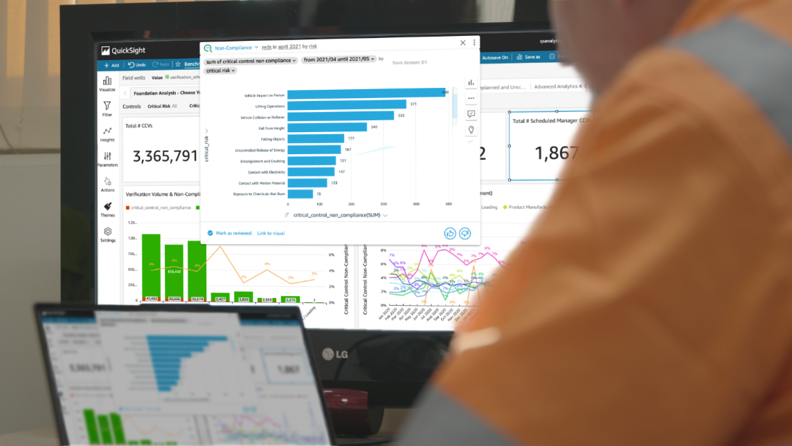
Shaheer Mansoor is a Data Scientist at AWS. His focus is on building machine learning platforms that can host AI solutions at scale. His interest areas are ML Ops, Feature Stores, Model Hosting and Model Monitoring.

Vadym Dolinin is a Machine Learning Architect in SumUp. He works with several teams on crafting the ML platform, which enables data scientists to build, deploy, and operate machine learning solutions in SumUp. Vadym has 13 years of experience in the domains of data engineering, analytics, BI, and ML.

Oliver Zollikofer is a Data Scientist at AWS. He enables global enterprise customers to build and deploy machine learning models, as well as architect related cloud solutions.

Leverage L2 constructs to reduce the complexity of your AWS CDK application

Post Syndicated from David Boldt original https://aws.amazon.com/blogs/devops/leverage-l2-constructs-to-reduce-the-complexity-of-your-aws-cdk-application/

The AWS Cloud Development Kit (AWS CDK) is an open-source software development framework to define your cloud application resources using familiar programming languages. AWS CDK uses the familiarity and expressive power of programming languages for modeling your applications. Constructs are the basic building blocks of AWS CDK apps. A construct represents a “cloud component” and encapsulates everything that AWS CloudFormation needs to create the component. Furthermore, AWS Construct Library lets you ease the process of building your application using predefined templates and logic. Three levels of constructs exist:

  • L1 – These are low-level constructs called Cfn (short for CloudFormation) resources. They’re periodically generated from the AWS CloudFormation Resource Specification. The name pattern is CfnXyz, where Xyz is name of the resource. When using these constructs, you must configure all of the resource properties. This requires a full understanding of the underlying CloudFormation resource model and its corresponding attributes.
  • L2 – These represent AWS resources with a higher-level, intent-based API. They provide additional functionality with defaults, boilerplate, and glue logic that you’d be writing yourself with L1 constructs. AWS constructs offer convenient defaults and reduce the need to know all of the details about the AWS resources that they represent. This is done while providing convenience methods that make it simpler to work with the resources and as a result creating your application.
  • L3 – These constructs are called patterns. They’re designed to complete common tasks in AWS, often involving multiple types of resources.

In this post, I show a sample architecture and how the complexity of an AWS CDK application is reduced by using L2 constructs.

Overview of the sample architecture

This solution uses Amazon API Gateway, AWS Lambda, and Amazon DynamoDB. I implement a simple serverless web application. The application receives a POST request from a user via API Gateway and forwards it to a Lambda function using proxy integration. The Lambda function writes the request body to a DynamoDB table.

The sample code can be found on GitHub.

The sample code can be found on GitHub.

Walkthrough

You can follow the instructions in the README file of the GitHub repository to deploy the stack. In the following walkthrough, I explain each logical unit and the differences when implementing it using L1 and L2 constructs. Before each code sample, I’ll show the path in the GitHub repository where you can find its source.

Create the DynamoDB table

First, I create a DynamoDB table to store the request content.

L1 construct

With L1 constructs, I must define each attribute of a table separately. For the DynamoDB table, these are keySchemaattributeDefinitions, and provisionedThroughput. They all require detailed CloudFormation knowledge, for example, how a keyType is defined.

lib/level1/database/infrastructure.ts

this.cfnDynamoDbTable = new dynamodb.CfnTable(
   this, 
   "CfnDynamoDbTable", 
   {
      keySchema: [
         {
            attributeName: props.attributeName,
            keyType: "HASH",
         },
      ],
      attributeDefinitions: [
         {
            attributeName: props.attributeName,
            attributeType: "S",
         },
      ],
      provisionedThroughput: {
         readCapacityUnits: 5,
         writeCapacityUnits: 5,
      },
   },
);

L2 construct

The corresponding L2 construct lets me use the default values for readCapacity (5) and writeCapacity (5). To further reduce the complexity, I define the attributes and the partition key simultaneously. In addition, I utilize the dynamodb.AttributeType.STRING enum.

lib/level2/database/infrastructure.ts

this.dynamoDbTable = new dynamodb.Table(
   this, 
   "DynamoDbTable", 
   {
      partitionKey: {
         name: props.attributeName,
         type: dynamodb.AttributeType.STRING,
      },
   },
);

Create the Lambda function

Next, I create a Lambda function which receives the request and stores the content in the DynamoDB table. The runtime code uses Node.js.

L1 construct

When creating a Lambda function using L1 construct, I must specify all of the properties at creation time – the business logic code location, runtime, and the function handler. This includes the role for the Lambda function to assume. As a result, I must provide the Attribute Resource Name (ARN) of the role. In the “Granting permissions” sections later in this post, I show how to create this role.

lib/level1/api/infrastructure.ts

const cfnLambdaFunction = new lambda.CfnFunction(
   this, 
   "CfnLambdaFunction", 
   {
      code: {
         zipFile: fs.readFileSync(
            path.resolve(__dirname, "runtime/index.js"),
            "utf8"
         ),
      },
      role: this.cfnIamLambdaRole.attrArn,
      runtime: "nodejs16.x",
      handler: "index.handler",
      environment: {
         variables: {
            TABLE_NAME: props.dynamoDbTableArn,
         },
      },
   },
);

L2 construct

I can achieve the same result with less complexity by leveraging the NodejsFunction L2 construct for Lambda function. It sets a default version for Node.js runtime unless another one is explicitly specified. The construct creates a Lambda function with automatic transpiling and bundling of TypeScript or Javascript code. This results in smaller Lambda packages that contain only the code and dependencies needed to run the function, and it uses esbuild under the hood. The Lambda function handler code is located in the runtime directory of the API logical unit. I provide the path to the Lambda handler file in the entry property. I don’t have to specify the handler function name, because the NodejsFunction construct uses the handler name by default. Moreover, a Lambda execution role isn’t required to be provided during L2 Lambda construct creation. If no role is specified, then a default one is generated which has permissions for Lambda execution. In the section ‘Granting Permissions’, I describe how to customize the role after creating the construct.

lib/level2/api/infrastructure.ts

this.lambdaFunction = new lambda_nodejs.NodejsFunction(
   this, 
   "LambdaFunction", 
   {
      entry: path.resolve(__dirname, "runtime/index.ts"),
      runtime: lambda.Runtime.NODEJS_16_X,
      environment: {
         TABLE_NAME: props.dynamoDbTableName,
      },
   },
);

Create API Gateway REST API

Next, I define the API Gateway REST API to receive POST requests with Cross-origin resource sharing (CORS) enabled.

L1 construct

Every step, from creating a new API Gateway REST API, to the deployment process, must be configured individually. With an L1 construct, I must have a good understanding of CORS and the exact configuration of headers and methods.

Furthermore, I must know all of the specifics, such as for the Lambda integration type I must know how to construct the URI.

lib/level1/api/infrastructure.ts

const cfnApiGatewayRestApi = new apigateway.CfnRestApi(
   this, 
   "CfnApiGatewayRestApi", 
   {
      name: props.apiName,
   },
);

const cfnApiGatewayPostMethod = new apigateway.CfnMethod(
   this, 
   "CfnApiGatewayPostMethod", 
   {
      httpMethod: "POST",
      resourceId: cfnApiGatewayRestApi.attrRootResourceId,
      restApiId: cfnApiGatewayRestApi.ref,
      authorizationType: "NONE",
      integration: {
         credentials: cfnIamApiGatewayRole.attrArn,
         type: "AWS_PROXY",
         integrationHttpMethod: "ANY",
         uri:
            "arn:aws:apigateway:" +
            Stack.of(this).region +
            ":lambda:path/2015-03-31/functions/" +
            cfnLambdaFunction.attrArn +
            "/invocations",
            passthroughBehavior: "WHEN_NO_MATCH",
      },
   },
);

const CfnApiGatewayOptionsMethod = new apigateway.CfnMethod(
    this,
    "CfnApiGatewayOptionsMethod",
   {    
      // fields omitted
   },
);

const cfnApiGatewayDeployment = new apigateway.CfnDeployment(
    this,
    "cfnApiGatewayDeployment",
    {
      restApiId: cfnApiGatewayRestApi.ref,
      stageName: "prod",
    },
);

L2 construct

Creating an API Gateway REST API with CORS enabled is simpler with L2 constructs. I can leverage the defaultCorsPreflightOptions property and the construct builds the required options method. To set origins and methods, I can use the apigateway.Cors enum. To configure the Lambda proxy option, all I need to do is to set the proxy variable in the method to true. A default deployment is created automatically.

lib/level2/api/infrastructure.ts

this.api = new apigateway.RestApi(
   this, 
   "ApiGatewayRestApi", 
   {
      defaultCorsPreflightOptions: {
         allowOrigins: apigateway.Cors.ALL_ORIGINS,
         allowMethods: apigateway.Cors.ALL_METHODS,
      },
   },
);

this.api.root.addMethod(
    "POST",
    new apigateway.LambdaIntegration(this.lambdaFunction, {
      proxy: true,
    })
);

Granting permissions

In the sample application, I must give permissions to two different resources:

  1.  API Gateway REST API to invoke the Lambda function.
  2. Lambda function to write data to the DynamoDB table.

L1 construct

For both resources, I must define AWS Identity and Access Management (IAM) roles. This requires in-depth knowledge of IAM, how policies are structured, and which actions are required. In the following code snippet, I start by creating the policy documents. Afterward, I create a role for each resource. These are provided at creation time to the corresponding constructs as shown earlier.

lib/level1/api/infrastructure.ts

const cfnLambdaAssumeIamPolicyDocument = {
    // fields omitted
};

this.cfnLambdaIamRole = new iam.CfnRole(
   this, 
   "cfnLambdaIamRole", 
   {
      assumeRolePolicyDocument: cfnLambdaAssumeIamPolicyDocument,
      managedPolicyArns: [
        "arn:aws:iam::aws:policy/service-role/AWSLambdaBasicExecutionRole",
      ],
   },
);
    
const cfnApiGatewayAssumeIamPolicyDocument = {
   // fields omitted
};

const cfnApiGatewayInvokeLambdaIamPolicyDocument = {
   Version: "2012-10-17",
   Statement: [
      {
         Action: ["lambda:InvokeFunction"],
         Resource: [cfnLambdaFunction.attrArn],
         Effect: "Allow",
      },
   ],
};

const cfnApiGatewayIamRole = new iam.CfnRole(
   this, 
   "cfnApiGatewayIamRole", 
   {
      assumeRolePolicyDocument: cfnApiGatewayAssumeIamPolicyDocument,
      policies: [{
         policyDocument: cfnApiGatewayInvokeLambdaIamPolicyDocument,
         policyName: "ApiGatewayInvokeLambdaIamPolicy",
      }],
   },
);

The database construct exposes a function to grant write access to any IAM role. The function creates a policy, which allows dynamodb:PutItem on the database table and adds it as an additional policy to the role.

lib/level1/database/infrastructure.ts

grantWriteData(cfnIamRole: iam.CfnRole) {
   const cfnPutDynamoDbIamPolicyDocument = {
      Version: "2012-10-17",
      Statement: [
         {
            Action: ["dynamodb:PutItem"],
            Resource: [this.cfnDynamoDbTable.attrArn],
            Effect: "Allow",
         },
      ],
   };

    cfnIamRole.policies = [{
        policyDocument: cfnPutDynamoDbIamPolicyDocument,
        policyName: "PutDynamoDbIamPolicy",
    }];
}

At this point, all permissions are in place, except that Lambda function doesn’t have permissions to write data to the DynamoDB table yet. To grant write access, I call the grantWriteData function of the Database construct with the IAM role of the Lambda function.

lib/deployment.ts

database.grantWriteData(api.cfnLambdaIamRole)

L2 construct

Creating an API Gateway REST API with the LambdaIntegration construct generates the IAM role and attaches the role to the API Gateway REST API method. Giving the Lambda function permission to write to the DynamoDB table can be achieved with the following single line:

lib/deployment.ts

database.dynamoDbTable.grantWriteData(api.lambdaFunction);

Using L3 constructs

To reduce complexity even further, I can leverage L3 constructs. In the case of this sample architecture, I can utilize the LambdaRestApi construct. This construct uses a default Lambda proxy integration. It automatically generates a method and a deployment, and grants permissions. As a result, I can achieve the same with even less code.

const restApi = new apigateway.LambdaRestApi(
   this, 
   "restApiLevel3", 
   {
      handler: this.lambdaFunction,
      defaultCorsPreflightOptions: {
         allowOrigins: apigateway.Cors.ALL_ORIGINS,
         allowMethods: apigateway.Cors.ALL_METHODS
      },
   },
);

Cleanup

Many services in this post are available in the AWS Free Tier. However, using this solution may incur costs, and you should tear down the stack if you don’t need it anymore. Cleanup steps are included in the RADME file of the GitHub repository.

Conclusion

In this post, I highlight the difference between using L1 and L2 AWS CDK constructs with an example architecture. Leveraging L2 constructs reduces the complexity of your application by using predefined patterns, boiler plate, and glue logic. They offer convenient defaults and reduce the need to know all of the details about the AWS resources they represent, while providing convenient methods that make it simpler to work with the resource. Additionally, I showed how to reduce complexity for common tasks even further by using an L3 construct.

Visit the AWS CDK documentation to learn more about building resilient, scalable, and cost-efficient architectures with the expressive power of a programming language.

Author:

David Boldt

David Boldt is a Solutions Architect at AWS, based in Hamburg, Germany. David works with customers to enable them with best practices in their cloud journey. He is passionate about the internet of Things and how it can be leveraged to solve different challenges across industries.

Tighten your package security with CodeArtifact Package Origin Control toolkit

Post Syndicated from Davide Semenzin original https://aws.amazon.com/blogs/devops/tighten-your-package-security-with-codeartifact-package-origin-control-toolkit/

Introduction

AWS CodeArtifact is a fully managed artifact repository service that makes it easy for organizations to securely store and share software packages used for application development. On Jul14 2022 we introduced a new feature called Package Origin Controls which allows customers to protect themselves against “dependency substitution“ or “dependency confusion” attacks.

This class of supply chain attacks can be carried out when an attacker with knowledge of an organization’s internally published package names (for example: Sample-Package=1.0.0) is able to publish such name(s) in a public repository. Package managers contain dependency resolution logic that pulls the latest version of a package. The attacker abuses this logic by publishing a high version number of a package with the same name as the organization’s package (for example: Sample-Package=99.0.0). The package manager then would resolve any requests for that package by pulling the attacker’s package version with malicious code instead of the internally published dependency.

In order for this type of attack to be successful, the organization must source their package versions from both internal and remote repositories at the same time. For example, your pip installation could be configured with multiple package indexes, both internal and external; or, as a CodeArtifact user you may have both the repository containing your private packages as well as an external connection to PyPI in the upstream graph of your current repository. In either case, the package manager is able to obtain package versions from more than one source. This causes the package manager to resolve the higher version number from the remote repository, instead of the trusted internal version.

A few strategies can be used to mitigate this kind of mixing: a simple one is to instruct the package manager to only source from an internal repository. While effective, this is often not practical, because it either significantly degrades developer experience or requires a lot of effort in order to set up, maintain, and vet external dependencies. Another mitigation consists in using explicit version pinning, which is also effective, though it might re-introduce the dependency substitution risk upon dependency upgrade without manual vetting. Some package managers also support namespaces or other types of dependency scoping, which are also helpful in preventing this class of attacks, but when available may not always actionable for existing packages due to the large amount of work required to do the renaming.

CodeArtifact is adding another tool to strengthen your software supply chain by introducing per-package per-repository controls which allow you to more precisely configure and control how package versions are sourced. For each package in your repository, you are now able to decide whether to allow or block sourcing versions from both upstream sources and direct publishing. These flags enable you to prevent mixed versions scenarios for all the types of packages supported by CodeArtifact without the need for additional package manager configuration.

While packages retained or published after the launch of this feature come with tighter-by-default origin configurations, in keeping with the principle of least astonishment we decided not to apply any of these policies retroactively. Therefore, your existing packages in CodeArtifact will not have their origin configuration changed and your setup will continue to work continue to work as it did before the feature was released.

Should you want to leverage this feature to tighten the security posture of your existing packages, we are releasing a toolkit to make it easier to bulk-set policy values in your repositories. This blog post describes how to use it.

Solution overview

The purpose of the Package Origin Control toolkit is to provide repository administrators with an easy way to set Origin Control policies in bulk on packages that have not received the default protection because they pre-date feature release. This can be achieved by blocking upstream versions for internal packages. In this blog post we will focus on this use-case, though the toolkit does support blocking publishing package versions to avoid a potentially vulnerable mixed state for external packages as well.

The toolkit is comprised of two scripts: a first one called generate_package_configurations.py for creating a manifest file listing the packages in a domain alongside their proposed origin configuration to apply, and a second one named apply_package_configurations.py, that reads the manifest file and applies the configuration within.

generate_package_configurations.py can operate on a whole repository, or on a subset of packages (specified either via filters, or though a list) and supports two origin control resolution modes:

  • A manual one where you supply the origin configuration you would like to set for all packages in scope. This is a good option if, for instance, you already maintain a list of internal packages, or if they are published in a consistent internal namespace which allows for them to be easily selected.
  • An automated one, which tries to identify what packages should have their upstreams blocked by analyzing the upstream repository graph and external connections, looking for evidence that package versions are only available from the repository at hand- in which case it determines it can disable sourcing of upstream versions can be done without risk of breaking builds. This is a good option if you want a quick way to tighten your security posture without having to manually analyze your whole repository.

With the manifest created, apply_package_configurations.py takes it as an input and effects the changes specified in it by calling the new PutPackageOriginConfiguration API (link). Precisely because it is meant to set these values in bulk, this script supports backup and revert operations by default, as well as dry-run and step-by-step confirmation options. If you identify an issue after applying origin control changes, you will be able to safely revert to the original, working configuration before trying again.

In this blog post we will cover how to use these tools:

  • To block package versions from upstream sources for all recommended packages in a repository
  • To block upstreams for a list of packages you already have
  • To revert to the original state in case of an incorrect configuration push

Prerequisites

The following prerequisites are required before you begin:

  1. Set up the Package Origin Control toolkit as described in the README on GitHub. You will need a working installation of Python 3.6 or later as well as the ability to install dependencies like the Python AWS SDK. The AWS CLI is not required.
  2. Write permissions on the CodeArtifact repository where you want to add package origin controls (see this link for additional info.)

Procedures

To block package versions from upstream sources for all recommended packages in a repository

Introduction

This procedure should be considered if you have a CodeArtifact repository with a variety of package formats and upstreams, and you want to have the toolkit automatically resolve what packages are safe to block upstreams for. It will block acquisition of new versions from upstreams only if two conditions are met:

  • the target repository doesn’t have access to an external connection
  • no versions of the package are available via any of its upstream repositories (either because the target repository itself doesn’t have any upstreams or because none of the upstreams have the package).

Therefore, we assume there isn’t an immediate External Connection attached to the target repository for the package format(s) you are trying to run this script against (because in that case the script would fall back on leaving things as-is for all packages).

Steps

  1. Make sure you have completed the required prerequisites described above
  2. Identify the target repository in your domain you want to automatically apply origin controls for, e.g. myrepo
  3. Identify the query parameters that define the list of packages you want to target. The script supports the same filters as the ListPackagesAPI.
    1. To match all packages in a repo, run :  python generate_package_configurations.py --region us-west-2 --domain mydomain --repository myrepo
      Please note that you always need to specify the AWS region and CodeArtifact domain alongside the repository.
    2. To match only some packages in a repo, for example only Python packages whose name begins with “internal_software_”:  python generate_package_configurations.py --region us-west-2 --domain mydomain --repository myrepo --format pypi --prefix internal_software_*
  4. If necessary, you can review the produced manifest file, which you will be able to find in the same folder under the name origin-configuration_mydomain_myrepo.csv (unless you have specified a different filename and path via the --output-file option)
  5. If the manifest file looks correct, you can apply the changes by calling the second stage: python apply_package_configurations.py --region us-west-2 --domain mydomain --repository myrepo --input origin-configuration_mydomain_myrepo.csv

To block package versions from upstream sources for all packages in a repository matching a list you maintain

Introduction

This procedure should be considered if you have a set of packages within your repository you know you want to apply origin control restrictions to. Rather than relying on a query, you can use such a list as an input to create a manifest.

Steps

Create a file containing a list of package names (and package names only). Multiple namespaces and formats are not supported and you will need to re-run this procedure for each. The expected file format is one package name per line. In this example we will want to block upstreams for three packages of the npm format (format is always mandatory when specifying a list of packages). As an example, a small input file is going to look something like this:

requests
numpy
django

(more information about this option can be found in the README)

Generate the manifest by supplying this file to the first stage, alongside the desired origin control configuration. In this case, we want to block upstreams for all packages in the supplied list (for more information about the origin control configuration string, consult the documentation): python generate_package_configurations.py --region us-west-2 --domain mydomain --repository myrepo --format npm --from-list inputfile.csv --set-restrictions publish=ALLOW,upstream=BLOCK

If necessary, you can review the produced manifest file, which you will be able to find in the same folder under the name origin-configuration_mydomain_myrepo.csv (unless you have specified a different filename and path via the –output-file option)

Run the apply_package_configurations.py script to update the package origin controls in your repository: apply_package_configurations.py --region us-west-2 --domain mydomain --repository myrepo --input origin-configuration_mydomain_myrepo.csv

To revert to the original state in case of an incorrect configuration push

Introduction

Erroneously bulk-changing your origin configuration can lead to broken builds and confusing failure modes for developers. To mitigate this risk, the toolkit backs up the existing configuration before making any changes and lets you easily revert them if need be.

Steps

Identify the manifest containing the configuration you want to revert. The toolkit automatically creates a backup file t for every input manifest you provide. This is the file produced by the first stage, which by default takes a name like origin-configuration_[domain]_[repository], for example origin-configuration_mydomain_myrepo.csv
Run the second stage script in restore mode:  python apply_package_configurations.py --region us-west-2 --domain mydomain --repository myrepo --input origin-configuration_mydomain_myrepo.csv --restore

Conclusion

In this blog post we have explained how to use the Origin Control toolkit to improve package security, focusing on restricting upstream package versions. We have demonstrated both an automated repository-wide application of the toolkit, which tries to minimize the amount of repository administrator work by applying a restriction heuristic, as well as a manual mode where a repository administrator can effect fine-grained origin control changes. Finally, we showed how these changes can be reverted using the built-in backup feature.

Author:

Davide Semenzin

Davide is a Software Development Engineer on the CodeArtifact team at Amazon Web Services (AWS). Previously he has worked at the Internet Archive building the infrastructure to digitize a million books per year. His interests are distributed systems, platform engineering and mission-critical high availability software. In his free time he likes to read books, fly airplanes, fly on airplanes, think about rockets and play with lasers.

Automating Amazon EC2-Windows EBS Volumes monitoring and creating alarms

Post Syndicated from Sheila Busser original https://aws.amazon.com/blogs/compute/automating-amazon-ec2-windows-ebs-volumes-monitoring-and-creating-alarms/

This blog post is written by, Santhosh Kumar Adapa, Database Consultant,  AWS WWCO ProServe,  Jeevan Shetty, Database Consultant, AWS WWCO ProServe, and Bhanu Ganesh Gudivada, Consultant  Databases, AWS WWCO ProServe.

Customers who are running fleets of Amazon Elastic Compute Cloud (Amazon EC2) instances use advanced monitoring techniques to observe their operational performance. Capabilities like aggregated and custom dimensions help customers categorize and customize their metrics across server fleets for fast and efficient decision making. Customers require visibility into not only infrastructure metrics (such as CPU and memory), but also disk usage metrics.

Monitoring Amazon EC2-Windows Amazon Elastic Block Store (Amazon EBS) Volumes usage is critical, especially when customers have a large fleet of Amazon EC2 Windows servers running to host their databases and applications in AWS. Generally, we see issues with EC2 instances running out of disk space, and free disk space isn’t a metric that is directly available with Amazon CloudWatch. Amazon CloudWatch agent helps solve this problem. After installing and configuring the CloudWatch agent on your EC2 instance, the agent will send metric data with the disk utilization to CloudWatch. The next step is to create a CloudWatch alarm to monitor the disk utilization metric.

In this post, we showcase the steps to automate the monitoring and creating alarms for EBS volumes attached to Amazon EC2 Windows instances. Alarms are created using AWS Lambda that monitors the free disk space and alerts whenever thresholds are crossed using Amazon Simple Notification Service (Amazon SNS).

Solution overview

To demonstrate the solution we first install and configure the CloudWatch agent in your Amazon EC2 Windows instance, and then the agent will send metric data with the disk utilization to CloudWatch. To monitor the disk on each Amazon EC2 Windows instance, we’ll use two custom Metrics, “FreeStorageSpaceInMB” and “FreeStorageSpaceInPercent”, that are collected by CloudWatch agent and pushed to CloudWatch.

The following diagram illustrates the architecture used in this post:

architecture used in this post

  1. Amazon EC2 Windows instance with attached Amazon EBS Volumes to be monitored for free disk usage. The EC2 instance is configured with Amazon CloudWatch Agent.
  2. CloudWatch agent is configured to monitor the “FreeStorageSpaceInMB” and “FreeStorageSpaceInPercent” metrics, and pushed to AWS CloudWatch.
  3. Lambda function that can be invoked to create CloudWatch alarms for each disk attached to the EC2 instance.
  4. CloudWatch Alarms are created with warnings and critical thresholds based on storage size.
  5. Amazon SNS is used to send alerts when the CloudWatch Alarms crosses the threshold.
  6. AWS Identity and Access Management (IAM) to provide permission to the Lambda function to get Amazon EBS metrics and to create CloudWatch Alarms.

Prerequisites

You will need the following prerequisites:

  • To implement this solution, you must have an Amazon EC2 Windows instance configured with Amazon CloudWatch Agent by following the steps documented in the article – How to monitor Windows and Linux servers and get internal performance metrics.
  • To monitor the “FreeStorageSpaceInMB” and “FreeStorageSpaceInPercent” metrics for Amazon EBS volumes attached to the EC2 instance, the CloudWatch agent configuration JSON should have the following section:
"LogicalDisk": {
	"measurement": [
	{
		"name":"% Free Space",
		"rename":"FreeStorageSpaceInPercent",
		"unit":"Percent"
	},
	{
		"name":"Free Megabytes",
		"rename":"FreeStorageSpaceInMB",
		"unit":"Megabytes"
	}
	],
	"metrics_collection_interval": 10,
	"resources": [
		"*"
	]
},
  1. Amazon EC2 host or bastion host with an IAM role attached that has permissions to create an IAM role, Lambda function, and run Amazon Relational Database Service (Amazon RDS) CLI commands. A Lambda function and an IAM role are created using AWS Serverless Application Model (SAM).

AWS SAM

In this section, we provide the steps to create an IAM role and deploy a Lambda function using AWS SAM.

  1. Log in to the Amazon EC2 host and install the AWS SAM CLI.
  2. Download the source code and deploy it by running the following command:
git clone https://github.com/aws-samples/aws-ec2-windows-ebs-volumes-monitoring

cd aws-ec2-windows-ebs-volumes-monitoring/ebs_volumes_monitoring
sam deploy --guided

3. Provide the following parameters:

    1. Stack Name – Name for the AWS CloudFormation stack.
    2. AWS Region – AWS Region where the stack is being deployed.

The following is the sample output when you run sam deploy –guided with default arguments:

=========================================
Stack Name [ebs-volumes-monitoring]: ebs-volumes-monitoring
AWS Region [us-west-2]:
#Shows you resources changes to be deployed and require a 'Y' to initiate deploy
Confirm changes before deploy [y/N]:
#SAM needs permission to be able to create roles to connect to the resources in your template
Allow SAM CLI IAM role creation [Y/n]:
#Preserves the state of previously provisioned resources when an operation fails
Disable rollback [y/N]:
Save arguments to configuration file [Y/n]:
SAM configuration file [samconfig.toml]:
SAM configuration environment [default]:

In the following sections, we describe the AWS services deployed with AWS SAM.

IAM role

AWS SAM creates an IAM role with policies to describe EC2 instances, as well as List, Get, and Put CloudWatch metrics. Furthermore, it attaches an AWS managed IAM policy called AWSLambdaBasicExecutionRole to the IAM role. This role is attached to the Lambda functions to create Amazon EBS volume alarms for EC2 instances.

Lambda function

AWS SAM also deploys the Lambda function. It uses Python 3.8 and accepts two parameters:

  1. Hostname: Amazon EC2 Windows instance name, or, if we must configure alarms for multiple servers, then you can use a wild card character, such as Instance_name* or Instance_name?
  2. sns_topic_name: ARN of the SNS topic that is used to configure CloudWatch Alarms. Notification is sent to the SNS topic when the Amazon EBS Volume metric crosses the threshold.

Invoking Lambda function

After the SAM deployment is successful, we can invoke the Lambda function with the instance name and the SNS Topic ARN. The Lambda function creates two alarms (Warning and Critical) for every Amazon EBS volume attached to the instance. The Warning and Critical values can be changed in the Lambda code so that there are two different values depending on the size of the disk drive. Furthermore, the alarms are configured to send notifications to the SNS Topic. The following is the sample command to invoke the Lambda function:

aws lambda invoke --function-name ec2-ebs-metric --cli-binary-format raw-in-base64-out \
--payload '{"hostname": "Windows*", "sns_topic_name": "arn:aws:sns:us-west-2:123456789:notify_dba" }' response.json

Verifying CloudWatch Alarms:

Verify the CloudWatch Alarms that are created in the CloudWatch console. The following screenshot shows the CloudWatch alarms created for an EC2 instance with four disks. There are two alarms (Warning and Critical) created for every disk (four disks in total). Therefore, we see eight CloudWatch alarms.

CloudWatch console alarms

Checking CloudWatch Logs:

After running the Lambda function, to verify the log, go to Lambda Service page, select the Lambda function created, navigate to the Monitor tab, and then select “View logs in CloudWatch”. Then, go to the latest log file to check the CloudWatch log files for any errors.

Checking CloudWatch LogsSelect the latest Log Steam to check the details of the last Lambda function execution.

Log Steam detailsThe log file shows the full details of the Lambda function execution. Furthermore, it shows the CloudWatch alarms configured for each disk, as well as if there are any errors generated during execution.

Log file detailsCleanup

To clean up the resources used in this post, complete the following steps:

  1. Delete the CloudFormation stack by running below command and replacing STACK_NAME with stack name provided in step 3a above, under section “AWS SAM”
sam delete --stack-name STACK_NAME
  1. Confirm the stack has been deleted by running below command. Replace STACK_NAME as mentioned in previous step.
aws cloudformation list-stacks --query "StackSummaries[?contains(StackName,' STACK_NAME ')].StackStatus"
  1. Delete any CloudWatch alarms created by the Lambda function by following the document – Editing or deleting a CloudWatch alarm.

Conclusion

In this post, we demonstrated how the requirement of monitoring Amazon EC2 Windows EBS Volumes usage is critical. In particular, this is essential when customers have a large fleet of Amazon EC2 Windows servers running to host their databases and applications in the cloud. We showcased the process of automating the free disk monitoring using Lambda and notifying through Amazon SNS when disks cross the storage threshold. By implementing such monitoring, customers can prevent issues with EC2 instances running out of disk space thus preventing critical production outages.

Provide any thoughts or questions in the comments section. We also encourage you to explore CloudWatch monitoring and try out additional use cases mentioned in the documentation.

How to Mitigate Docker Hub’s pull rate limit error through AWS Code build and ECR

Post Syndicated from Bijith Nair original https://aws.amazon.com/blogs/devops/how-to-mitigate-docker-hubs-pull-rate-limit-error-through-aws-code-build-and-ecr/

How to mitigate Docker Hub’s pull rate limit errors

Docker, Inc. has announced that its hosted repository service, Docker Hub, will begin limiting the rate at which the Docker images are being pulled. The pull rate limit will purely be based on the individual IP Address. The anonymous user can do 100 pulls per 6 hours per IP Address, while the authenticated user can do 200 pulls per 6 hours.

This post shows how you can overcome those errors while you’re working with AWS Developer Tools, such as AWS CodeCommit, AWS CodeBuild, and Amazon Elastic Container Registry (Amazon ECR).

Solution overview

The workflow and architecture of the solution work as follows:

  1. The developer will push the code, in this case (buildspec, Dockerfile, README.md) to CodeCommit by using Git client installed locally.
  2. CodeBuild will pull the latest commit id from CodeCommit.
  3. CodeBuild will build the base Docker image by going through the build steps listed in buildspec and Dockerfile.

Finally, Docker image will be pushed to Amazon ECR, and it can be used for future deployments.

AWS Services Overview:

Architectural Overview - Leverage AWS Developer tools to mitigate Docker hub's pull rate limit error

Figure 1. Architectural Overview – Leverage AWS Developer tools to mitigate Docker hub’s pull rate limit error.

For this post, we’ll be using the following AWS services

  • AWS CodeCommit – a fully-managed source control service that hosts secure Git-based repositories.
  • AWS CodeBuild – a fully managed continuous integration service that compiles source code, runs tests, and produces software packages that are ready to deploy.
  • Amazon ECR – an AWS managed container image registry service that is secure, scalable, and reliable.

Prerequisites

The prerequisites, before we build the pipeline, are as follows:

Setup Amazon ECR repositories

We’ll be setting up two Amazon ECR repositories. The first repository, “golang”, will hold the base image which we will be migrating from Docker hub. And the second repository, “mydemorepo”, will hold the final image for your sample application.

ECR Repositories with Source and Target image

Figure 2. ECR Repositories with Source and Target image.

Migrate your existing Docker image from Docker Hub to Amazon ECR

Note that for this post, I’ll be using golang:1.12-alpine as the base Docker image to be migrated to Amazon ECR.

Once you have your base repository setup, the next step is to pull the golang:1.12-alpine public image from docker hub to you laptop/Server.

To do that, log in to your local server where you have deployed all of the prerequisites. This includes the Docker engine, Git Client, AWS CLI, etc., and run the following command:

docker pull golang:1.12-alpine

Authenticate to your Amazon ECR private registry, and click here to learn more about private registry authentication.

aws ecr get-login-password --region us-east-1 | docker login --username AWS --password-stdin 12345678910.dkr.ecr.us-east-1.amazonaws.com

Apply the appropriate Tag to your image.

docker tag golang:1.12-alpine 12345678910.dkr.ecr.us-east-1.amazonaws.com/golang:1.12-alpine

Push your image to the Amazon ECR repository.

docker push 150359982618.dkr.ecr.us-east-1.amazonaws.com/golang:1.12-alpine

The Source Image

Figure 3. The Source Image.

Once your image gets pushed to Amazon ECR with all of the required tags, the next step is to use this base image as the source image to build our sample application. Furthermore, while going through the “Overview of the Solution” section, you might have noticed that we must have a source code repository for CodeBuild to fetch the latest code from, and to build a sample application. Let’s go through how to set up your source code repository.

Set up a source code repository using CodeCommit

Let’s start by setting up the repository name. In this case, let’s call it “mysampleapp”. Keep rest of the settings as is, and then select create.

Screenshot for creating a repository under AWS Code Commit

Figure 4. Screenshot for creating a repository under AWS Code Commit.

Once the repository gets created, go to the top-right corner. Under Clone URL, select Clone HTTPS.

Clone URL to copy the code Locally on your desktop or server

Figure 5. Clone URL to copy the code Locally on your desktop or server.

Go back to your local server or laptop where you want to clone the repo, and authenticate your repository. Learn more about how to HTTPS connections to AWS Codecommit repositories.

git clone https://git-codecommit.us-east-1.amazonaws.com/v1/repos/mysampleapp mysampleapp

Note that you have your empty repository cloned locally with a folder name “mysampleapp”. The next step is to set up Dockerfile and buildspec.

Set up a Dockerfile and buildspec for building the base image of your Sample Application

To build a Docker image, we’ll set up three files under the “mysampleapp” folder.

Buildspec.yml
Dockerfile
README.md

List out the base code pushed to AWS Code commit

Figure 6. List out the base code pushed to AWS Code commit.

Note that I have also listed the content inside of buildspec.yml, Dockerfile, and ReadME.md in case you want a sample code to test the scenario.

buildspec.yml

version: 0.2
phases:
pre_build:
commands:
- echo Logging in to Amazon ECR...
- REPOSITORY_URI=12345678910.dkr.ecr.us-east-1.amazonaws.com/mydemorepo
- AWS_DEFAULT_REGION=us-east-1
- AWS_ACCOUNT_ID=12345678910
- aws ecr get-login-password --region $AWS_DEFAULT_REGION | docker login --username AWS --password-stdin $AWS_ACCOUNT_ID.dkr.ecr.$AWS_DEFAULT_REGION.amazonaws.com
- IMAGE_REPO_NAME=mydemorepo
- COMMIT_HASH=$(echo $CODEBUILD_RESOLVED_SOURCE_VERSION | cut -c 1-7)
- IMAGE_TAG=build-$(echo $CODEBUILD_BUILD_ID | awk -F":" '{print $2}')
build:
commands:
- echo Build started on `date`
- echo Building the Docker image...
- docker build -t $REPOSITORY_URI:latest .
- docker images
- docker tag $REPOSITORY_URI:latest $REPOSITORY_URI:$IMAGE_TAG
post_build:
commands:
- echo Build completed on `date`
- echo Pushing the Docker image...
- docker push $REPOSITORY_URI:latest
- docker push $REPOSITORY_URI:$IMAGE_TAG

Dockerfile

Point your Dockfile to use Amazon ECR repository instead of Docker hub.

FROM golang:1.12-alpine AS build << Replace the public Image with ECR private image

FROM 150359982618.dkr.ecr.us-east-1.amazonaws.com/golang: 1.12-alpine

AS build

#Install git

RUN apk add --no-cache git

#Get the hello world package from a GitHub repository

RUN go get github.com/golang/example/hello

WORKDIR /go/src/github.com/golang/example/hello

#Build the project and send the output to /bin/HelloWorld

RUN go build -o /bin/HelloWorld

README.md

> Demo Repository has files related to CodeBuild spec and Dockerfile

* buildspec.yaml
* Dockerfile

Now, commit your changes locally, and push them to Amazon ECR. Note that to learn more about how to set up HTTPS users using Git Credentials, click here.

git add .
git commit -m "My First Commit - Sample App"
git push -u origin master

Now, go back to your AWS Management Console, and Under Developer Tools, select CodeCommit. Go to mysampleapp, and you should see three files with the latest commits.

Screenshot with buildspec, Dockerfile and README.

Figure 7. Screenshot with buildspec, Dockerfile and README

That concludes our setup to CodeCommit. Next, we’ll set up a build project.

Set up a CodeBuild project

Enter the project name, in this case let’s use “mysamplbuild”.

Setting up a Build Project.

Figure 8. Setting up a Build Project.

Select the provider as CodeCommit, followed by the repository and the branch that contains the latest commit.

Selecting the source code provider which is Code Commit and the source repository.

Figure 9.  Selecting the source code provider which is Code Commit and the source repository.

Select the runtime as standard, and then choose the latest Amazon Linux image. Make sure that the environment type is set to Linux. Privileged option should be checked. For the rest of the options, go with the defaults.

Required environment variables and attributes.

Figure 10.  Required environment variables and attributes.

Choose the buildspec.

Figure 11.  Choose the buildspec.

Once the project gets created, select the project, and select start Build.

Screenshot of the build project along with details.

Figure 12. Screenshot of the build project along with details.

Once you trigger the build, you will notice that CodeBuild is pulling the image from Amazon ECR instead of Docker hub.

The log file for the build.

Figure 13. The log file for the build.

Clean up

To avoid incurring future charges, delete the resources.

Conclusion

Developers can use AWS to host both their private and public container images. This decreases the need to use different public websites and registries. Public images will be geo-replicated for reliable availability around the world, and they’ll offer fast downloads to quickly serve up images on-demand. Anyone (with or without an AWS account) will be able to browse and pull containerized software for use in their own applications.

Author:

Bijith Nair

Bijith Nair is a Solutions Architect at Amazon Web Services, Based out of Dallas, Texas. He helps customers architect, develop, scalable and highly available solutions to support their business innovation.

Accelerate machine learning with AWS Data Exchange and Amazon Redshift ML

Post Syndicated from Yadgiri Pottabhathini original https://aws.amazon.com/blogs/big-data/accelerate-machine-learning-with-aws-data-exchange-and-amazon-redshift-ml/

Amazon Redshift ML makes it easy for SQL users to create, train, and deploy ML models using familiar SQL commands. Redshift ML allows you to use your data in Amazon Redshift with Amazon SageMaker, a fully managed ML service, without requiring you to become an expert in ML.

AWS Data Exchange makes it easy to find, subscribe to, and use third-party data in the cloud. AWS Data Exchange for Amazon Redshift enables you to access and query tables in Amazon Redshift without extracting, transforming, and loading files (ETL).

As a subscriber, you can browse through the AWS Data Exchange catalog and find data products that are relevant to your business with data stored in Amazon Redshift, and subscribe to the data from the providers without any further processing, and no need for an ETL process.

If the provider data is not already available in Amazon Redshift, many providers will add the data to Amazon Redshift upon request.

In this post, we show you the process of subscribing to datasets through AWS Data Exchange without ETL, running ML algorithms on an Amazon Redshift cluster, and performing local inference and production.

Solution overview

The use case for the solution in this post is to predict ticket sales for worldwide events based on historical ticket sales data using a regression model. The data or ETL engineer can build the data pipeline by subscribing to the Worldwide Event Attendance product on AWS Data Exchange without ETL. You can then create the ML model in Redshift ML using the time series ticket sales data and predict future ticket sales.

To implement this solution, you complete the following high-level steps:

  1. Subscribe to datasets using AWS Data Exchange for Amazon Redshift.
  2. Connect to the datashare in Amazon Redshift.
  3. Create the ML model using the SQL notebook feature of the Amazon Redshift query editor V2.

The following diagram illustrates the solution architecture.

Prerequisites

Before starting this walkthrough, you must complete the following prerequisites:

  1. Make sure you have an existing Amazon Redshift cluster with RA3 node type. If not, you can create a provisioned Amazon Redshift cluster.
  2. Make sure the Amazon Redshift cluster is encrypted, because the data provider is encrypted and Amazon Redshift data sharing requires homogeneous encryption configurations. For more details on homogeneous encryption, refer to Data sharing considerations in Amazon Redshift.
  3. Create an AWS Identity Access and Management (IAM) role with access to SageMaker and Amazon Simple Storage Service (Amazon S3) and attach it to the Amazon Redshift cluster. Refer to Cluster setup for using Amazon Redshift ML for more details.
  4. Create an S3 bucket for storing the training data and model output.

Please note that some of the above AWS resources in this walkthrough will incur charges. Please remember to delete the resources when you’re finished.

Subscribe to an AWS Data Exchange product with Amazon Redshift data

To subscribe to an AWS Data Exchange public dataset, complete the following steps:

  1. On the AWS Data Exchange console, choose Explore available data products.
  2. In the navigation pane, under Data available through, select Amazon Redshift to filter products with Amazon Redshift data.
  3. Choose Worldwide Event Attendance (Test Product).
  4. Choose Continue to subscribe.
  5. Confirm the catalog is subscribed by checking that it’s listed on the Subscriptions page.

Predict tickets sold using Redshift ML

To set up prediction using Redshift ML, complete the following steps:

  1. On the Amazon Redshift console, choose Datashares in the navigation pane.
  2. On the Subscriptions tab, confirm that the AWS Data Exchange datashare is available.
  3. In the navigation pane, choose Query editor v2.
  4. Connect to your Amazon Redshift cluster in the navigation pane.

Amazon Redshift provides a feature to create notebooks and run your queries; the notebook feature is currently in preview and available in all Regions. For the remaining part of this tutorial, we run queries in the notebook and create comments in the markdown cell for each step.

  1. Choose the plus sign and choose Notebook.
  2. Choose Add markdown.
  3. Enter Show available data share in the cell.
  4. Choose Add SQL.
  5. Enter and run the following command to see the available datashares for the cluster:
    SHOW datashares;

You should be able to see worldwide_event_test_data, as shown in the following screenshot.

  1. Note the producer_namespace and producer_account values from the output, which we use in the next step.
  2. Choose Add markdown and enter Create database from datashare with producer_namespace and procedure_account.
  3. Choose Add SQL and enter the following code to create a database to access the datashare. Use the producer_namespace and producer_account values you copied earlier.
    CREATE DATABASE ml_blog_db FROM DATASHARE worldwide_event_test_data OF ACCOUNT 'producer_account' NAMESPACE 'producer_namespace';

  4. Choose Add markdown and enter Create new table to consolidate features.
  5. Choose Add SQL and enter the following code to create a new table called event consisting of the event sales by date and assign a running serial number to split into training and validation datasets:
    CREATE TABLE event AS
    	SELECT eventname, qtysold, saletime, day, week, month, qtr, year, holiday, ROW_NUMBER() OVER (ORDER BY RANDOM()) r
    	FROM "ml_blog_db"."public"."sales" s
    	INNER JOIN "ml_blog_db"."public"."event" e
    	ON s.eventid = e.eventid
    	INNER JOIN "ml_blog_db"."public"."date" d
    	ON s.dateid = d.dateid;

Event name, quantity sold, sale time, day, week, month, quarter, year, and holiday are columns in the dataset from AWS Data Exchange that are used as features in the ML model creation.

  1. Choose Add markdown and enter Split the dataset into training dataset and validation dataset.
  2. Choose Add SQL and enter the following code to split the dataset into training and validation datasets:
    CREATE TABLE training_data AS 
    	SELECT eventname, qtysold, saletime, day, week, month, qtr, year, holiday
    	FROM event
    	WHERE r >
    	(SELECT COUNT(1) * 0.2 FROM event);
    
    	CREATE TABLE validation_data AS 
    	SELECT eventname, qtysold, saletime, day, week, month, qtr, year, holiday
    	FROM event
    	WHERE r <=
    	(SELECT COUNT(1) * 0.2 FROM event);

  3. Choose Add markdown and enter Create ML model.
  4. Choose Add SQL and enter the following command to create the model. Replace the your_s3_bucket parameter with your bucket name.
    CREATE MODEL predict_ticket_sold
    	FROM training_data
    	TARGET qtysold
    	FUNCTION predict_ticket_sold
    	IAM_ROLE 'default'
    	PROBLEM_TYPE regression
    	OBJECTIVE 'mse'
    	SETTINGS (s3_bucket 'your_s3_bucket',
    	s3_garbage_collect off,
    	max_runtime 5000);

Note: It can take up to two hours to create and train the model.
The following screenshot shows the example output from adding our markdown and SQL.

  1. Choose Add markdown and enter Show model creation status. Continue to next step once the Model State has changed to Ready.
  2. Choose Add SQL and enter the following command to get the status of the model creation:
    SHOW MODEL predict_ticket_sold;

Move to the next step after the Model State has changed to READY.

  1. Choose Add markdown and enter Run the inference for eventname Jason Mraz.
  2. When the model is ready, you can use the SQL function to apply the ML model to your data. The following is sample SQL code to predict the tickets sold for a particular event using the predict_ticket_sold function created in the previous step:
    SELECT eventname,
    	predict_ticket_sold(
    	eventname, saletime, day, week, month, qtr, year, holiday ) AS predicted_qty_sold,
    	day, week, month
    	FROM event
    	Where eventname = 'Jason Mraz';

The following is the output received by applying the ML function predict_ticket_sold on the original dataset. The output of the ML function is captured in the field predicted_qty_sold, which is the predicted ticket sold quantity.

Share notebooks

To share the notebooks, complete the following steps:

  1. Create an IAM role with the managed policy AmazonRedshiftQueryEditorV2FullAccess attached to the role.
  2. Add a principal tag to the role with the tag name sqlworkbench-team.
  3. Set the value of this tag to the principal (user, group, or role) you’re granting access to.
  4. After you configure these permissions, navigate to the Amazon Redshift console and choose Query editor v2 in the navigation pane. If you haven’t used the query editor v2 before, please configure your account to use query editor v2.
  5. Choose Notebooks in the left pane and navigate to My notebooks.
  6. Right-click on the notebook you want to share and choose Share with my team.
  7. You can confirm that the notebook is shared by choosing Shared to my team and checking that the notebook is listed.

Summary

In this post, we showed you how to build an end-to-end pipeline by subscribing to a public dataset through AWS Data Exchange, simplifying data integration and processing, and then running prediction using Redshift ML on the data.

We look forward to hearing from you about your experience. If you have questions or suggestions, please leave a comment.


About the Authors

Yadgiri Pottabhathini is a Sr. Analytics Specialist Solutions Architect. His role is to assist customers in their cloud data warehouse journey and help them evaluate and align their data analytics business objectives with Amazon Redshift capabilities.

Ekta Ahuja is an Analytics Specialist Solutions Architect at AWS. She is passionate about helping customers build scalable and robust data and analytics solutions. Before AWS, she worked in several different data engineering and analytics roles. Outside of work, she enjoys baking, traveling, and board games.

BP Yau is a Sr Product Manager at AWS. He is passionate about helping customers architect big data solutions to process data at scale. Before AWS, he helped Amazon.com Supply Chain Optimization Technologies migrate its Oracle data warehouse to Amazon Redshift and build its next generation big data analytics platform using AWS technologies.

Srikanth Sopirala is a Principal Analytics Specialist Solutions Architect at AWS. He is a seasoned leader with over 20 years of experience, who is passionate about helping customers build scalable data and analytics solutions to gain timely insights and make critical business decisions. In his spare time, he enjoys reading, spending time with his family, and road cycling.

Configuring low latency connectivity between AWS Outposts rack and on-premises data using CoIP

Post Syndicated from Sheila Busser original https://aws.amazon.com/blogs/compute/configuring-low-latency-connectivity-between-aws-outposts-rack-using-coip-and-on-premises-data/

This blog post is written by, Leonardo Azize Martins, Cloud Infrastructure Architect, Professional Services.

AWS Outposts rack enables applications that need to run on-premises due to low latency, local data processing, or local data storage needs by connecting Outposts rack to your on-premises network via the local gateway (LGW).

Each Outpost rack includes a local gateway to provide low latency connectivity between the Outpost and any local data sources, end users, local machinery and equipment, or local databases. If you have an Outpost rack, you can include a local gateway as the target in your VPC subnet route table where the destination is your on-premises network. Local gateways are only available for Outposts rack and can only be used in route tables where the VPC has been associated with an LGW.

In a previous blog post on connecting AWS Outposts to on-premises data sources, you learned the different use cases to use AWS Outposts connected with your local network. In this post, you will dive deep into local gateway usage and specific details about it. You will learn how to use Outpost local gateway when it is configured as Customer-owned IP addresses (CoIP) mode. You will also learn how to integrate it with your Amazon Virtual Private Cloud (Amazon VPC) and how different routes work regarding Amazon Elastic Compute Cloud (Amazon EC2) instances running on Outposts.

Overview of solution

The primary role of a local gateway is to provide connectivity from an Outpost to your local on-premises LAN. It also provides AWS Outposts connectivity to the internet through your on-premises network via the LGW, so you don’t need to rely on an internet gateway (IGW). The local gateway can also provide a data plane path back to the AWS Region. If you already have connectivity between your LAN and the Region through AWS Site-to-Site VPN or AWS Direct Connect, you can use the same path to connect from the Outpost to the AWS Region privately.

Outpost subnet

Public subnets and private subnets are important concepts to understand for Outposts networking. A public subnet has a route to an internet gateway. The same concept applies to Outpost subnets, when a public subnet exists on Outposts, it will have a route to an internet gateway, which will use a service link as a communication path between an Outpost and the internet gateway in the parent AWS Region.

Outpost public route via internet gateway

A private subnet does not have a direct route to the internet gateway. It will only be local inside the VPC, or it could have a route to a Network Address Translation (NAT) gateway. In both cases, the communication between Outpost subnets and AWS Region subnets will be done via the service link.

Outpost private route via NAT gateway

Your subnet can be private and only be allowed to communicate with your on-premises network. You just need a route pointing to the LGW.

Outpost private route via LGW

You can also provide internet connectivity to your Outpost subnets via LGW. In this case, it will not use the service link. As soon as it traverses the LGW and goes to your next hop, it will follow your routing flow to the internet.

Outpost public route via LGW

Routing

By default, every Outpost subnet inherits the main route table from its VPC. You can create a custom route table and associate it with an Outpost subnet. You can include a local gateway as the target when the destination is your on-premises network. A local gateway can only be used in VPC and subnet route tables that are exclusively associated with an Outpost subnet. If the route table is associated with an Outpost subnet and a Region subnet, it will not allow you to add a local gateway as the target.

Error message: addition of a local gateway as the target is denied

Local gateways are also not supported in the main route table.

Error message: routes that target local gateways not supported in main route table

The local gateway advertises Outpost IP address ranges to your on-premises network via BGP. In the other direction, from an on-premises network to the Outpost, it doesn’t use BGP, which means there is no propagation. You need to configure your VPC route table with static routes.

As of this writing, the LGW does not support jumbo frame.

Outposts IP addresses

Outposts can be configured in customer-owned IP (CoIP) mode.

Customer-owned IP

During the installation process, uses information that you provide about your on-premises network to create an address pool, which is known as a customer-owned IP address pool (CoIP pool). AWS then assigns it to the local gateway for use and advertises back to your on-premises network through BGP.

CoIP addresses provide local or external connectivity to resources in your Outpost subnets through your on-premises network. You can assign these IP addresses to resources on your Outpost, such as an EC2 instance, by allocating a new Elastic IP address from the customer-owned IP pool and then assigning this new Elastic IP address to your EC2 instance.

A local gateway serves as NAT for EC2 instances that have been assigned addresses from your customer-owned IP pool.

You can optionally share your customer-owned pool with multiple AWS accounts in your AWS Organizations using the AWS Resource Access Manager (RAM). After you share the pool, participants can allocate and associate Elastic IP addresses from the customer-owned IP pool.

Communication between your Outpost and on-premises network will use the CoIP Elastic IP addresses to address instances in the Outpost; the VPC CIDR range is not used.

Walkthrough

You will follow the steps required to configure your VPC to use LGW configured as CoIP, including:

  • Associate your VPC with the LGW route table.
  • Create an Outposts subnet.
  • Create and associate the VPC route table with the subnet.
  • Add a route to on-premises network with LGW as the target.

Prerequisites

For this walkthrough, you should have the following prerequisites:

  • An AWS account.
  • An Outpost that consists of one or more Outposts racks configured in CoIP mode.

Associate VPC with LGW route table

Use the following procedure to associate a VPC with the LGW route table. You can’t associate VPCs that have a CIDR block conflict.

  1. Open the AWS Outposts console.
  2. In the navigation pane, choose Local gateway route tables.
  3. Select the route table and then choose Actions, Associate VPC.
  4. For VPC ID, select the VPC to associate with the local gateway route table.
  5. Choose Associate VPC.

Create an Outpost subnet

You can add Outpost subnets to any VPC in the parent AWS Region for the Outpost. When you do so, the VPC also spans the Outpost.

  1. Open the AWS Outposts console.
  2. On the navigation pane, choose Outposts.
  3. Select the Outpost, and then choose Actions, Create subnet.
  4. Select the VPC and specify an IP address range for the subnet.
  5. Choose Create.

Create and associate VPC route table with the Outpost subnet

You can create a custom route table for your VPC using the Amazon VPC console. It is a best practice to have one specific route table for each subnet.

  1. Open the Amazon VPC console.
  2. In the navigation pane, choose Route Tables.
  3. Choose Create route table.
  4. For VPC, choose your VPC.
  5. Choose Create.
  6. On the Subnet associations tab, choose Edit subnet associations.
  7. Select the check box for the subnet to associate with the route table and then choose Save associations.

Add a route to on-premises network with LGW as the target

You can add a route to a route table using the Amazon VPC console.

  1. Open the Amazon VPC console.
  2. In the navigation pane, choose Route Tables and select
  3. Choose Actions, Edit routes.
  4. Choose Add route. For Destination, enter the destination CIDR block, a single IP address, or the ID of a prefix list.
  5. Choose Save routes.

Allocate and associate a customer-owned IP address

  1. Open the Amazon EC2 console.
  2. In the navigation pane, choose Elastic IPs.
  3. Choose Allocate new address.
  4. For Network Border Group, select the location from which the IP address is advertised.
  5. For Public IPv4 address pool, choose Customer owned IPv4 address pool.
  6. For Customer owned IPv4 address pool, select the pool that you configured.
  7. Choose Allocate and close the confirmation screen.
  8. In the navigation pane, choose Elastic IPs.
  9. Select an Elastic IP address and choose Actions, Associate address.
  10. Select the instance from Instance and then choose Associate.

For more information about Launch an instance on your Outpost, refer to the AWS Outposts User Guide.

Allocate Elastic IP address

Cleaning up

To avoid incurring future charges, delete the resources, like EC2 instances.

Conclusion

In this post, I covered how to use the Outposts rack local gateway to communicate with your on-premises network. You learned how a subnet route table can influence the connectivity of public or private Outpost instances.

To learn more, check out our Outposts local gateway documentation and the networking reference architecture.