Real-time anomaly detection describes a use case to detect and flag unexpected behavior in streaming data as it occurs. Online machine learning (ML) algorithms are popular for this use case because they don’t require any explicit rules and are able to adapt to a changing baseline, which is particularly useful for continuous streams of data where incoming data changes continuously over time.
Random Cut Forest (RCF) is one such algorithm widely used for anomaly detection use cases. In typical setups, we want to be able to run the RCF algorithm on input data with large throughput, and streaming data processing frameworks can help with that. We are excited to share that RCF is possible with Amazon Kinesis Data Analytics for Apache Flink. Apache Flink is a popular open-source framework for real-time, stateful computations over data streams, and can be used to run RCF on input streams with large throughput.
This post demonstrates how we can use Kinesis Data Analytics for Apache Flink to run an online RCF algorithm for anomaly detection.
Solution overview
The following diagram illustrates our architecture, which consists of three components: an input data stream using Amazon Kinesis Data Streams, a Flink job, and an output Kinesis data stream. In terms of data flow, we use a Python script to generate anomalous sine wave data into the input data stream, the data is then processed by RCF in a Flink job, and the resultant anomaly score is delivered to the output data stream.
The following graph shows an example of our expected result, which indicates that the anomaly score peaked when the sine wave data source anomalously dropped to constant -17.
We can implement this solution in three simple steps:
Set up a data generator to produce data into the source data stream.
Run the RCF Flink Java code on Kinesis Data Analytics.
Set up AWS resources via AWS CloudFormation
The following CloudFormation stack will create all the AWS resources we need for this tutorial, including two Kinesis data streams, a Kinesis Data Analytics app, and an Amazon Simple Storage Service (Amazon S3) bucket.
Sign in to your AWS account, then choose Launch Stack:
Follow the steps on the AWS CloudFormation console to create the stack.
Set up a data generator
Run the following Python script to populate the input data stream with the anomalous sine wave data:
import json
import boto3
import math

STREAM_NAME = "ExampleInputStream-RCF"


def get_data(time):
    rad = (time/100)%360
    val = math.sin(rad)*10 + 10

    if rad > 2.4 and rad < 2.6:
        val = -17

    return {'time': time, 'value': val}

def generate(stream_name, kinesis_client):
    time = 0

    while True:
        data = get_data(time)
        kinesis_client.put_record(
            StreamName=stream_name,
            Data=json.dumps(data),
            PartitionKey="partitionkey")

        time += 1


if __name__ == '__main__':
    generate(STREAM_NAME, boto3.client('kinesis', region_name='us-west-2'))
Run the RCF Flink Java code on Kinesis Data Analytics
The CloudFormation stack automatically downloaded and packaged the RCF Flink job JAR file for you. Therefore, you can simply go to the Kinesis Data Analytics console to run your application.
That’s it! We now have a running Flink job that continuously reads in data from an input Kinesis data stream and calculates the anomaly score for each new data point given the previous data points it has seen.
The following sections explain the RCF implementation and Flink job code in more detail.
RCF implementation
Numerous RCF implementations are publicly available. For this tutorial, we use the AWS implementation by wrapping it around a custom wrapper (RandomCutForestOperator) to be used in our Flink job.
RandomCutForestOperator is implemented as an Apache Flink ProcessFunction, which is a function that allows us to write custom logic to process every element in the stream. Our custom logic starts with a data transformation via inputDataMapper.apply, followed by getting the anomaly score by calling the AWS RCF library via rcf.getAnomalyScore. The code implementation of RandomCutForestOperator can be found on GitHub.
RandomCutForestOperatorBuilder requires two main types of parameters:
RandomCutForestOperatorhyperparameters – We use the following:
Dimensions – We set this to 1 because our input data is a 1-dimensional sine wave consisting of the float data type.
ShingleSize – We set this to 1, which means our RCF algorithm will take into account the previous and current data points in anomaly score deduction. Note that this can be increased to account for seasonality in data.
SampleSize – We set this to 628, which means a maximum of 628 data points is kept in the data sample for each tree.
DataMapper parameters for input and output processing – We use the following:
InputDataMapper – We use RandomCutForestOperator.SIMPLE_FLOAT_INPUT_DATA_MAPPER to map input data from float to float[].
ResultMapper – We use RandomCutForestOperator.SIMPLE_TUPLE_RESULT_DATA_MAPPER, which is a BiFunction that joins the anomaly score with the corresponding sine wave data point into a tuple.
Flink job code
The following code snippet illustrates the core streaming structure of our Apache Flink streaming Java code. It first reads in data from the source Kinesis data stream, then processes it using the RCF algorithm. The computed anomaly score is then written to an output Kinesis data stream.
In this example, our baseline input data is a sine wave. As shown in the following screenshot, a low anomaly score is returned when the data is regular. However, when there is an anomaly in the data (when the sine wave input data drops to a constant), a high anomaly score is returned. The anomaly score is delivered into an output Kinesis data stream. You can visualize this result by creating a Kinesis Data Analytics Studio app; for instructions, refer to Interactive analysis of streaming data.
Because this is an unsupervised algorithm, you don’t need to provide any explicit rules or labeled datasets for this operator. In short, only the input data stream, data conversions, and some hyperparameters were provided. The RCF algorithm itself determined the expected baseline based on the input data and identified any unexpected behavior.
Furthermore, this means the model will continuously adapt even if the baseline changes over time. As such, minimal retraining cadence is required. This is powerful for anomaly detection on streaming data because the data will often drift slowly over time due seasonal trends, inflation, equipment calibration drift, and so on.
Clean up
To avoid incurring future charges, complete the following steps:
On the Amazon S3 console, empty the S3 bucket created by the CloudFormation stack.
On the AWS CloudFormation console, delete the CloudFormation stack.
Conclusion
This post demonstrated how to perform anomaly detection on input streaming data with RCF, an online unsupervised ML algorithm using Kinesis Data Analytics. We also showed how this algorithm learns the data baseline on its own, and can adapt to changes in the baseline over time. We hope you consider this solution for your real-time anomaly detection use cases.
About the Authors
Daren Wong is a Software Development Engineer in AWS. He works on Amazon Kinesis Data Analytics, the managed offering for running Apache Flink applications on AWS.
Aleksandr Pilipenko is a Software Development Engineer in AWS. He works on Amazon Kinesis Data Analytics, the managed offering for running Apache Flink applications on AWS.
Hong Liang Teoh is a Software Development Engineer in AWS. He works on Amazon Kinesis Data Analytics, the managed offering for running Apache Flink applications on AWS.
AWS Glue is a serverless data integration service that makes it simple to discover, prepare, and combine data for analytics, machine learning (ML), and application development. You can use AWS Glue to create, run, and monitor data integration and ETL (extract, transform, and load) pipelines and catalog your assets across multiple data stores.
One of the most common questions we get from customers is how to effectively monitor and optimize costs on AWS Glue for Spark. The diversity of features and pricing options for AWS Glue offers the flexibility to effectively manage the cost of your data workloads and still keep the performance and capacity as per your business needs. Although the fundamental process of cost optimization for AWS Glue workloads remains the same, you can monitor job runs and analyze the costs and usage to find savings and take action to implement improvements to the code or configurations.
In this post, we demonstrate a tactical approach to help you manage and reduce cost through monitoring and optimization techniques on top of your AWS Glue workloads.
Monitor overall costs on AWS Glue for Apache Spark
AWS Glue for Apache Spark charges an hourly rate in 1-second increments with a minimum of 1 minute based on the number of data processing units (DPUs). Learn more in AWS Glue Pricing. This section describes a way to monitor overall costs on AWS Glue for Apache Spark.
AWS Cost Explorer
In AWS Cost Explorer, you can see overall trends of DPU hours. Complete the following steps:
On the Cost Explorer console, create a new cost and usage report.
For Service, choose Glue.
For Usage type, choose the following options:
Choose <Region>-ETL-DPU-Hour (DPU-Hour) for standard jobs.
Choose <Region>-ETL-Flex-DPU-Hour (DPU-Hour) for Flex jobs.
Choose <Region>-GlueInteractiveSession-DPU-Hour (DPU-Hour) for interactive sessions.
This section describes a way to monitor individual job run costs on AWS Glue for Apache Spark. There are two options to achieve this.
AWS Glue Studio Monitoring page
On the Monitoring page in AWS Glue Studio, you can monitor the DPU hours you spent on a specific job run. The following screenshot shows three job runs that processed the same dataset; the first job run spent 0.66 DPU hours, and the second spent 0.44 DPU hours. The third one with Flex spent only 0.33 DPU hours.
GetJobRun and GetJobRuns APIs
The DPU hour values per job run can be retrieved through AWS APIs.
For auto scaling jobs and Flex jobs, the field DPUSeconds is available in GetJobRun and GetJobRuns API responses:
For these jobs, you can calculate DPU hours by ExecutionTime*MaxCapacity/(60*60). Then you get 0.44 DPU hour by 157*10/(60*60)=0.44. Note that AWS Glue versions 2.0 and later have a 1-minute minimum billing.
AWS CloudFormation template
Because DPU hours can be retrieved through the GetJobRun and GetJobRuns APIs, you can integrate this with other services like Amazon CloudWatch to monitor trends of consumed DPU hours over time. For example, you can configure an Amazon EventBridge rule to invoke an AWS Lambda function to publish CloudWatch metrics every time AWS Glue jobs finish.
To help you configure that quickly, we provide an AWS CloudFormation template. You can review and customize it to suit your needs. Some of the resources this stack deploys incur costs when in use.
The CloudFormation template generates the following resources:
Per-job run metrics – Dimension=[JobName, JobRunId]
Aggregated metrics and per-job metrics are shown as in the following screenshot.
Each datapoint represents DPUHours per individual job run, so valid statistics for the CloudWatch metrics is SUM. With the CloudWatch metrics, you can have a granular view on DPU hours.
Options to optimize cost
This section describes key options to optimize costs on AWS Glue for Apache Spark:
Upgrade to the latest version
Auto scaling
Flex
Set the job’s timeout period appropriately
Interactive sessions
Smaller worker type for streaming jobs
We dive deep to the individual options.
Upgrade to the latest version
Having AWS Glue jobs running on the latest version enables you to take advantage of the latest functionalities and improvements offered by AWS Glue and the upgraded version of the supported engines such as Apache Spark. For example, AWS Glue 4.0 includes the new optimized Apache Spark 3.3.0 runtime and adds support for built-in pandas APIs as well as native support for Apache Hudi, Apache Iceberg, and Delta Lake formats, giving you more options for analyzing and storing your data. It also includes a new highly performant Amazon Redshift connector that is 10 times faster on TPC-DS benchmarking.
Auto scaling
One of the most common challenges to reduce cost is to identify the right amount of resources to run jobs. Users tend to overprovision workers in order to avoid resource-related problems, but part of those DPUs are not used, which increases costs unnecessarily. Starting with AWS Glue version 3.0, AWS Glue auto scaling helps you dynamically scale resources up and down based on the workload, for both batch and streaming jobs. Auto scaling reduces the need to optimize the number of workers to avoid over-provisioning resources for jobs, or paying for idle workers.
To enable auto scaling on AWS Glue Studio, go to the Job Details tab of your AWS Glue job and select Automatically scale number of workers.
For non-urgent data integration workloads that don’t require fast job start times or can afford to rerun the jobs in case of a failure, Flex could be a good option. The start times and runtimes of jobs using Flex vary because spare compute resources aren’t always available instantly and may be reclaimed during the run of a job. Flex-based jobs offer the same capabilities, including access to custom connectors, a visual job authoring experience, and a job scheduling system. With the Flex option, you can optimize the costs of your data integration workloads by up to 34%.
To enable Flex on AWS Glue Studio, go to the Job Details tab of your job and select Flex execution.
One common practice among developers that create AWS Glue jobs is to run the same job several times every time a modification is made to the code. However, this may not be cost-effective depending of the number of workers assigned to the job and the number of times that it’s run. Also, this approach may slow down the development time because you have to wait until every job run is complete. To address this issue, in 2022 we released AWS Glue interactive sessions. This feature let developers process data interactively using a Jupyter-based notebook or IDE of their choice. Sessions start in seconds and have built-in cost management. As with AWS Glue jobs, you pay for only the resources you use. Interactive sessions allow developers to test their code line by line without needing to run the entire job to test any changes made to the code.
Set the job’s timeout period appropriately
Due to configuration issues, script coding errors, or data anomalies, sometimes AWS Glue jobs can take an exceptionally long time or struggle to process the data, and it can cause unexpected charges. AWS Glue gives you the ability to set a timeout value on any jobs. By default, an AWS Glue job is configured with 48 hours as the timeout value, but you can specify any timeout. We recommend identifying the average runtime of your job, and based on that, set an appropriate timeout period. This way, you can control cost per job run, prevent unexpected charges, and detect any problems related to the job earlier.
To change the timeout value on AWS Glue Studio, go to the Job Details tab of your job and enter a value for Job timeout.
Interactive sessions also have the same ability to set an idle timeout value on sessions. The default idle timeout value for Spark ETL sessions is 2880 minutes (48 hours). To change the timeout value, you can use %idle_timeout magic.
Smaller worker type for streaming jobs
Processing data in real time is a common use case for customers, but sometimes these streams have sporadic and low data volumes. G.1X and G.2X worker types could be too big for these workloads, especially if we consider streaming jobs may need to run 24/7. To help you reduce costs, in 2022 we released G.025X, a new quarter DPU worker type for streaming ETL jobs. With this new worker type, you can process low data volume streams at one-fourth of the cost.
To select the G.025X worker type on AWS Glue Studio, go to the Job Details tab of your job. For Type, choose Spark Streaming, then choose G 0.25X for Worker type.
Performance tuning plays an important role in reducing cost. The first action for performance tuning is to identify the bottlenecks. Without measuring the performance and identifying bottlenecks, it’s not realistic to optimize cost-effectively. CloudWatch metrics provide a simple view for quick analysis, and the Spark UI provides deeper view for performance tuning. It’s highly recommended to enable Spark UI for your jobs and then view the UI to identify the bottleneck.
The following are high-level strategies to optimize costs:
Scale cluster capacity
Reduce the amount of data scanned
Parallelize tasks
Optimize shuffles
Overcome data skew
Accelerate query planning
For this post, we discuss the techniques for reducing the amount of data scanned and parallelizing tasks.
Reduce the amount of data scanned: Enable job bookmarks
AWS Glue job bookmarks are a capability to process data incrementally when running a job multiple times on a scheduled interval. If your use case is an incremental data load, you can enable job bookmarks to avoid a full scan for all job runs and process only the delta from the last job run. This reduces the amount of data scanned and accelerates individual job runs.
Reduce the amount of data scanned: Partition pruning
If your input data is partitioned in advance, you can reduce the amount of data scan by pruning partitions.
For Spark DataFrame (or Spark SQL), set a where or filter clause to prune partitions:
# DataFrame
df = spark.read.format("json").load("s3://<YourBucket>/year=2023/month=03/*/*.gz")

# SparkSQL
df = spark.sql("SELECT * FROM <Table> WHERE year= '2023' and month = '03'")
Parallelize tasks: Parallelize JDBC reads
The number of concurrent reads from the JDBC source is determined by configuration. Note that by default, a single JDBC connection will read all the data from the source through a SELECT query.
Both AWS Glue DynamicFrame and Spark DataFrame support parallelize data scans across multiple tasks by splitting the dataset.
For Spark DataFrame, set numPartitions, partitionColumn, lowerBound, and upperBound. Learn more in JDBC To Other Databases.
Conclusion
In this post, we discussed methodologies for monitoring and optimizing cost on AWS Glue for Apache Spark. With these techniques, you can effectively monitor and optimize costs on AWS Glue for Spark.
If you have comments or feedback, please leave them in the comments.
About the Authors
Leonardo Gómez is a Principal Analytics Specialist Solutions Architect at AWS. He has over a decade of experience in data management, helping customers around the globe address their business and technical needs. Connect with him on LinkedIn
Noritaka Sekiyama is a Principal Big Data Architect on the AWS Glue team. He is responsible for building software artifacts to help customers. In his spare time, he enjoys cycling with his new road bike.
This is a guest post by Valdiney Gomes, Hélio Leal, and Flávia Lima from Dafiti.
Data and its various uses is increasingly evident in companies, and each professional has their preferences about which technologies to use to visualize data, which isn’t necessarily in line with the technological needs and infrastructure of a company. At Dafiti, a Brazilian fashion and style e-commerce retailer, it was no different. Five tools were used by different sectors of the company, which caused misalignment and management overhead, spreading our resources thin to support them. Looking for a tool that would enable us to democratize our data, we chose Amazon QuickSight, a cloud-native, serverless business intelligence (BI) service that powers interactive dashboards that lets us make better data-driven decisions, as a corporate solution for data visualization.
In this post, we discuss why we chose QuickSight and how we implemented it.
Why we chose QuickSight
We had specific requirements for our BI solution and looked at many different options. The following factors guided our decision:
Tool close to data – It was important to have the data visualization tool as close to the data as possible. At Dafiti, the entire infrastructure is on AWS, and we use Amazon Redshift as our Data Warehouse. QuickSight, when using SPICE (Super-fast, Parallel, In-memory Calculation Engine), extracts data from Amazon Redshift as efficiently as possible using UNLOAD, which optimizes the use of Amazon Redshift.
Highly available and accessible solution – We wanted to be able to be access the tool by web or mobile interface, in addition to being able to do almost anything through API calls.
Serverless solution – All the other data visualization solutions that were used at Dafiti were on premises, which created unnecessary cost and effort to maintain these services, taking the focus away from what was most important to us: data.
Flexible pricing model – We needed a pricing model that would allow us to provide access to everyone in the company and at a price defined by usage and not by license. Thanks to AWS pay-as-you-go pricing, with more than double the number of users we had on our previous main data visualization solution, our cost with QuickSight is about 10 times lower.
Robust documentation – The material provided by AWS proved to be helpful, allowing our team to put the project into production.
Unifying our solution
We were previously using Qlikview, Sisense, Tableau, SAP, and Excel to analyze our data across different teams. We were already using other AWS services and learning about QuickSight when we hosted a Data Battle with AWS, a hybrid event for more than 230 Dafiti employees. This event had a hands-on approach with a workshop followed by a friendly QuickSight competition. Participants had to get information in their own dashboard to answer correctly. This 5-hour event flew by, accelerated the learning path of technical and business teams, and proved that QuickSight was the right tool for us.
QuickSight has brought all of our teams into one tool, while lowering costs by 80% and enabling us to do so much more together. Currently, over 400 employees, including our CEO, across nine different business units are using QuickSight as their sole source of truth on a daily basis. This includes human resources, auditing, and customer service, which previously had their analyses spread across several sources.
Data democratization
Data democratization is one of Dafiti’s main objectives. We believe that allowing everyone to analyze the data, following Brazilian, Argentinean, and Colombian privacy laws, unlocks potential for improving decision-making processes by extracting value from the data generated by the company. However, the democratization of data comes with the responsible use of resources. Yes, we want all users to be able to access and extract value from the data, but the cost can never be greater than the value that this generates.
How we organized the project
Data democratization drives Dafiti’s strategy. When implementing QuickSight, the obsession of becoming an even more data-driven company (we talk about this at the AWS Summit SP 2022) and having data increasingly accessible was what guided the project.
We organized QuickSight by folders, as can be seen in the following figure, and each folder represents a business area. This makes it easier to grant access and ensures that all people from the same area have access to exactly the same set of data and reports.
In this model, people from the corporate data area can view and edit any resource from any area, while customer service users can view and edit resources only for customer service.
Expanding the model a bit, the reports created by one area can be shared with others, as can be seen in the following figure, in which the SAC report was shared with Support, creating what we call a reporting portfolio.
In this way, all users who join any of the groups will have exactly the same view as any of their peers, eliminating privileges in accessing data. In addition, the portfolio is enriched every day with reports that are created and maintained by other areas, but which may be of interest to areas other than the one responsible for creating it.
For this to work correctly, a certain rigidity is necessary in relation to the few naming and documentation standards that have been defined. On the other hand, designers have complete freedom to define the characteristics of their reports.
Another highlight in this model is that no report can be shared directly with a specific user; this restriction was defined using custom permissions in QuickSight. Therefore, the reports are always shared only through the folders. After all, we want the data to be accessible equally to everyone in the company.
Technical configurations
QuickSight offers a comprehensive API, and all the activities we carry out on a daily basis take place through these APIs. Among these activities, we highlight the granting of access and the monitoring of various aspects of the tool.
The QuickSight visual interface allows most of the tool’s maintenance activities to be performed and integration with Active Directory or the use of AWS Identity and Access Management (IAM) users is possible, but we understand that it wouldn’t be the ideal choice to grant access. Therefore, we defined an access grant flow for users and groups based on the QuickSight API, as can be seen in the following figure. In this model, the creation and removal of users is done through a JSON file with the following structure:
Whenever a user needs to be added or changed, the file is edited and a pull request is submitted to GitHub. If the request is approved, an action is triggered to send the file to an Amazon Simple Storage Service (Amazon S3) bucket. From this, an AWS Lambda function is triggered that performs two activities: the first is the maintenance of users and groups, and the second is the sending of an invitation through Amazon Simple Email Service (Amazon SES) for users to join QuickSight. In our case, we opted for a personalized invitation model that would emphasize the data democratization initiative that is being conducted.
To monitor the tool, we implemented the architecture shown in the following figure, in which we used AWS CloudTrail to pull out the QuickSight logs and the QuickSight API to extract information from the tool’s resources, such as reports, users, datasets, data sources, and more. All of this data is processed by Glove, our data integration tool, stored in Amazon Redshift, and analyzed in QuickSight itself. This allows us to understand the behavior of our users and concentrate efforts on the most-used resources, in addition to allowing optimal cost control and the use of SPICE.
To update the datasets, we don’t use the QuickSight internal scheduler, due to the large volume of data and the complexity of the DAGs. We prefer updating the datasets within our ETL (extract, transform, and load) and ELT process orchestration flow. For this purpose, we use Hanger, our orchestration tool. This approach allows the datasets to be updated only when the data source is changed and the data quality processes are executed. This model is represented by the following figure.
Conclusion
Choosing a data visualization tool is not a simple task. It involves many considerations, and several aspects must be analyzed in order for the choice to fit the characteristics of the company and to be consistent with the profile of business users.
For Dafiti, QuickSight was a natural choice from the moment we learned about its features. We needed a service that was in the same cloud as our main data sources, extremely fast using SPICE, and solved the maintenance and cost problem of on-premises applications. In terms of functionalities that are necessary for our business, it met our needs perfectly.
Do you want to know more about what we are doing in the data area here at Dafiti? Check out the following videos:
Valdiney Gomes is Data Engineering Coordinator at Dafiti. He worked for many years in software engineering, migrated to data engineering, and currently leads an amazing team responsible for the data platform for Dafiti in Latin America.
Hélio Leal is a Data Engineering Specialist at Dafiti, responsible for maintaining and evolving the entire data platform at Dafiti using AWS solutions.
Flávia Lima is a Data Engineer at Dafiti, responsible for sustaining the data platform and providing the data from many sources to internal customers.
Implementing an effective data sharing strategy that satisfies compliance and regulatory requirements is complex. Customers often need to share data between disparate software as a service (SaaS) platforms within their organization or across organizations. On many occasions, they need to apply business logic to the data received from the source SaaS platform before pushing it to the target SaaS platform.
Let’s take an example. AnyCompany’s marketing team hosted an event at the Anaheim Convention Center, CA. The marketing team created leads based on the event in Adobe Marketo. An automated process downloaded the leads from Marketo in the marketing AWS account. These leads are then pushed to the sales AWS account. A business process picks up those leads, filters them based on a “Do Not Call” criteria, and creates entries in the Salesforce system. Now, the sales team can pursue those leads and continue to track the opportunities in Salesforce.
Considering our example of AnyCompany, let’s look at the data flow. AnyCompany’s Marketo instance is integrated with the producer AWS account. As the leads from Marketo land in the producer AWS account, they’re pushed to the consumer AWS account, which is integrated to Salesforce. Business logic is applied to the leads data in the consumer AWS account, and then the curated data is loaded into Salesforce.
We have used a serverless architecture to implement this use case. The following AWS services are used for data ingestion, processing, and load:
Amazon AppFlow is a fully managed integration service that enables you to securely transfer data between SaaS applications like Salesforce, SAP, Marketo, Slack, and ServiceNow, and AWS services like Amazon S3 and Amazon Redshift, in just a few clicks. With AppFlow, you can run data flows at nearly any scale at the frequency you choose—on a schedule, in response to a business event, or on demand. You can configure data transformation capabilities like filtering and validation to generate rich, ready-to-use data as part of the flow itself, without additional steps. Amazon AppFlow is used to download leads data from Marketo and upload the curated leads data into Salesforce.
Amazon EventBridge is a serverless event bus that lets you receive, filter, transform, route, and deliver events. EventBridge is used to track the events like receiving the leads data in the producer or consumer AWS accounts and then triggering a workflow.
AWS Step Functions is a visual workflow service that helps developers use AWS services to build distributed applications, automate processes, orchestrate microservices, and create data and machine learning (ML) pipelines. Step Functions is used to orchestrate the data processing.
AWS Glue is a serverless data preparation service that makes it easy to run extract, transform, and load (ETL) jobs. An AWS Glue job encapsulates a script that reads, processes, and then writes data to a new schema. This solution uses Python 3.6 AWS Glue jobs for data filtration and processing.
Amazon Simple Storage Service (Amazon S3) is an object storage service offering industry-leading scalability, data availability, security, and performance. Amazon S3 is used to store the leads data.
Let’s review the architecture in detail. The following diagram shows a visual representation of how this integration works.
The following steps outline the process for transferring and processing leads data using Amazon AppFlow, Amazon S3, EventBridge, Step Functions, AWS Glue, and Salesforce:
Amazon AppFlow runs on a daily schedule and retrieves any new leads created within the last 24 hours (incremental changes) from Marketo.
The leads are saved as Parquet format files in an S3 bucket in the producer account.
When the daily flow is complete, Amazon AppFlow emits events to EventBridge.
EventBridge triggers Step Functions.
Step Functions copies the Parquet format files containing the leads from the producer account’s S3 bucket to the consumer account’s S3 bucket.
Upon a successful file transfer, Step Functions publishes an event in the consumer account’s EventBridge.
An EventBridge rule intercepts this event and triggers Step Functions in the consumer account.
Step Functions calls an AWS Glue crawler, which scans the leads Parquet files and creates a table in the AWS Glue Data Catalog.
The AWS Glue job is called, which selects records with the Do Not Call field set to false from the leads files, and creates a new set of curated Parquet files. We have used an AWS Glue job for the ETL pipeline to showcase how you can use purpose-built analytics service for complex ETL needs. However, for simple filtering requirements like Do Not Call, you can use the existing filtering feature of Amazon AppFlow.
Step Functions then calls Amazon AppFlow.
Finally, Amazon AppFlow populates the Salesforce leads based on the data in the curated Parquet files.
We have provided artifacts in this post to deploy the AWS services in your account and try out the solution.
Prerequisites
To follow the deployment walkthrough, you need two AWS accounts, one for the producer and other for the consumer. Use us-east-1 or us-west-2 as your AWS Region.
Consumer account setup:
Stage the data
To prepare the data, complete the following steps:
Download the zipped archive file to use for this solution and unzip the files locally.
The AWS Glue job uses the glue-job.py script to perform ETL and populates the curated table in the Data Catalog.
Create an S3 bucket called consumer-configbucket-<ACCOUNT_ID> via the Amazon S3 console in the consumer account, where ACCOUNT_ID is your AWS account ID.
Upload the script to this location.
Create a connection to Salesforce
Follow the connection setup steps outlined in here. Please make a note of the Salesforce connector name.
Create a connection to Salesforce in the consumer account
We provided two AWS CloudFormation templates to create resources: one for the producer account, and one for the consumer account.
Amazon S3 now applies server-side encryption with Amazon S3 managed keys (SSE-S3) as the base level of encryption for every bucket in Amazon S3. Starting January 5, 2023, all new object uploads to Amazon S3 are automatically encrypted at no additional cost and with no impact on performance. We use this default encryption for both producer and consumer S3 buckets. If you choose to bring your own keys with AWS Key Management Service (AWS KMS), we recommend referring to Replicating objects created with server-side encryption (SSE-C, SSE-S3, SSE-KMS) for cross-account replication.
Launch the CloudFormation stack in the consumer account
Let’s start with creating resources in the consumer account. There are a few dependencies on the consumer account resources from the producer account. To launch the CloudFormation stack in the consumer account, complete the following steps:
Sign in to the consumer account’s AWS CloudFormation console in the target Region.
Choose Launch Stack.
Choose Next.
For Stack name, enter a stack name, such as stack-appflow-consumer.
Enter the parameters for the connector name, object, and producer (source) account ID.
Choose Next.
On the next page, choose Next.
Review the details on the final page and select I acknowledge that AWS CloudFormation might create IAM resources.
Choose Create stack.
Stack creation takes approximately 5 minutes to complete. It will create the following resources. You can find them on the Outputs tab of the CloudFormation stack.
Review the details on the final page and select I acknowledge that AWS CloudFormation might create IAM resources.
Choose Create stack.
Stack creation takes approximately 5 minutes to complete. It will create the following resources. You can find them on the Outputs tab of the CloudFormation stack.
Producer Step Function – arn:aws:states:<region>:<producer account id>:stateMachine:ProducerStateMachine-xxxx
Producer Step Function Role – arn:aws:iam::<producer account id>:role/service-role/producer-stepfunction-role
After successful creation of the resources, go to the consumer account S3 bucket, consumer-databucket-<consumer account id>, and update the bucket policy as follows:
Review the Marketo and Salesforce connection setup in the producer and consumer account respectively.
In the architecture section, we suggested scheduling the AppFlow (producer-flow) in the producer account. However, for quick testing purposes, we demonstrate how to manually run the flow on demand.
Go to the AppFlow (producer-flow) in the producer account. On the Filters tab of the flow, choose Edit filters.
Choose the Created At date range for which you have data.
Save the range and choose Run flow.
Review the producer S3 bucket.
AppFlow generates the files in the producer-flow prefix within this bucket. The files are temporarily located in the producer S3 bucket under s3://<producer-bucket>.<region>.<account-id>/producer-flow.
Review the EventBridge rule and Step Functions state machine in the producer account.
The Amazon AppFlow job completion triggers an EventBridge rule (arn:aws:events:<region>:<producer account id>:rule/producer-appflow-completion-event, as noted in the Outputs tab of the CloudFromation stack in the Producer Account), which triggers the Step Functions state machine (arn:aws:states:<region>:<producer account id>:stateMachine:ProducerStateMachine-xxxx) in the producer account. The state machine copies the files to the consumer S3 bucket from the producer-flow prefix in the producer S3 bucket. Once file copy is complete, the state machine moves the files from the producer-flow prefix to the archive prefix in the producer S3 bucket. You can find the files in s3://<producer-bucket>.<region>.<account-id>/archive.
Review the consumer S3 bucket.
The Step Functions state machine in the producer account copies the files to the consumer S3 bucket and sends an event to EventBridge in the consumer account. The files are located in the consumer S3 bucket under s3://consumer-databucket-<account-id>/marketo-leads-source/.
Review the EventBridge rule (arn:aws:events:<region>:<consumer account id>:rule/consumer-custom-event-bus/consumer-custom-event-bus-rule) in the consumer account, which should have triggered the Step Function workflow (arn:aws:states:<region>:<consumer account id>:stateMachine:consumer-state-machine).
The AWS Glue crawler (consumer-glue-crawler) runs to update the metadata followed by the AWS Glue job (consumer-glue-job), which curates the data by applying the Do not call filter. The curated files are placed in s3://consumer-databucket-<account-id>/marketo-leads-curated/. After data curation, the flow is started as part of the state machine.
Review the Amazon AppFlow job (arn:aws:appflow:<region>:<consumer account id>:flow/consumer-appflow) run status in the consumer account.
Upon a successful run of the Amazon AppFlow job, the curated data files are moved to the s3://consumer-databucket-<account-id>/marketo-leads-processed/ folder and Salesforce is updated with the leads. Additionally, all the original source files are moved from s3://consumer-databucket-<account-id>/marketo-leads-source/ to s3://consumer-databucket-<account-id>/marketo-leads-archive/.
Review the updated data in Salesforce.
You will see newly created or updated leads created by Amazon AppFlow.
Clean up
To clean up the resources created as part of this post, delete the following resources:
Delete the resources in the producer account:
Delete the producer S3 bucket content.
Delete the CloudFormation stack.
Delete the resources in the consumer account:
Delete the consumer S3 bucket content.
Delete the CloudFormation stack.
Summary
In this post, we showed how you can support a cross-account model to exchange data between different partners with different SaaS integrations using Amazon AppFlow. You can expand this idea to support multiple target accounts.
Ramakant Joshi is an AWS Solutions Architect, specializing in the analytics and serverless domain. He has a background in software development and hybrid architectures, and is passionate about helping customers modernize their cloud architecture.
Debaprasun Chakraborty is an AWS Solutions Architect, specializing in the analytics domain. He has around 20 years of software development and architecture experience. He is passionate about helping customers in cloud adoption, migration and strategy.
Suraj Subramani Vineet is a Senior Cloud Architect at Amazon Web Services (AWS) Professional Services in Sydney, Australia. He specializes in designing and building scalable and cost-effective data platforms and AI/ML solutions in the cloud. Outside of work, he enjoys playing soccer on weekends.
Many of our customers use Amazon Cognito user pools to add authentication, authorization, and user management capabilities to their web and mobile applications. You can enable the built-in advanced security in Amazon Cognito to detect and block the use of credentials that have been compromised elsewhere, and to detect unusual sign-in activity and then prompt users for additional verification or block sign-ins. Additionally, you can associate an AWS WAF web access control list (web ACL) with your user pool to allow or block requests to Amazon Cognito user pools, based on security rules.
In this post, we’ll show how you can use AWS WAF with Amazon Cognito user pools and provide a sample set of rate-based rules and advanced AWS WAF rule groups. We’ll also show you how to test and tune the rules to help protect your user pools from common threats.
Rate-based rules for Amazon Cognito user pool endpoints
The following are endpoints exposed publicly by an Amazon Cognito user pool that you can protect with AWS WAF:
Public API operations — These generate a request to Cognito API actions that are either unauthenticated or authenticated with a session string or access token, but not with AWS credentials.
A good way to protect these endpoints is to deploy rate-based AWS WAF rules. These rules will detect and block requests with high rates that could indicate an attempt to exceed your Amazon Cognito API request rate quotas and that could subsequently impact requests from legitimate users.
When you apply rate limits, it helps to group Amazon Cognito API actions into four action categories. You can set specific rate limits per action category giving you traffic visibility for each category.
User Creation — This category includes operations that create new users in Cognito. Setting a rate limit for this category provides visibility for traffic of these operations and threats such as fake users being created in Cognito, which drives up your Monthly Active User (MAU) costs for Cognito.
Sign-in — This category includes operations to initiate a sign-in operation. Setting a rate limit for this category can provide visibility into the abuse of these operations. This could indicate high frequency, automated attempts to guess user credentials, sometimes referred to as credential stuffing.
Account Recovery — This category includes operations to recover accounts, including “forgot password” flows. Setting a rate limit for this category can provide visibility into the abuse of these operations, malicious activity can include: sending fake reset attempts, which might result in emails and SMS messages being sent to users.
Default — This is a catch-all rate limit that applies to an operation that is not in one of the prior categories. Setting a default rate limit can provide visibility and mitigation from request flooding attacks.
Table 1 below shows selected Hosted UI endpoint paths (the equivalent of individual API actions) and the recommended rate-based rule limit category for each.
Additionally, the rate-based rules we provide in this post include the following:
Two IP sets that represent allow lists for IPv4 and IPv6. You can add IPs that represent your trusted source IP addresses to these IP sets so that other AWS WAF rules don’t apply to requests that originate from these IP addresses.
Two IP sets that represent deny lists for IPv4 and IPv6. Add IPs to these IP sets that you want to block in all cases, regardless of the result of other rules.
An AWS managed IP reputation rule group: The AWS managed IP reputation list rule group contains rules that are based on Amazon internal threat intelligence, to identify IP addresses typically associated with bots or other threats. You can limit requests that match rules in this rule group to a specific rate limit.
Deploy rate-based rules
You can deploy the rate-based rules described in the previous section by using the AWS CloudFormation template that we provide here.
To deploy rate-based rules using the template
(Optional but recommended) If you want to enable AWS WAF logging and resources to analyze request rates, create an Amazon Simple Storage Service (Amazon S3) bucket in the same AWS Region as your Amazon Cognito user pool, with a bucket name starting with the prefix aws-waf-logs-. If you previously created an S3 bucket for AWS WAF logs, you can choose to reuse it, or you can create a new bucket to store AWS WAF logs for Amazon Cognito.
Choose the following Launch Stack button to launch a CloudFormation stack in your account.
Note: The stack will launch in the N. Virginia (us-east-1) Region. To deploy this solution into other AWS Regions, download the solution’s CloudFormation template and deploy it to the selected Region.
This template creates the following resources in your AWS account:
A rule group for the rate-based rules, according to the limits shown in Tables 1 and 2.
Four IP sets for an allow list and deny list for IPv4 and IPv6 addresses.
A web ACL that includes the rule group that is created, IP set based rules, and the AWS managed IP reputation rule group.
(Optional) The template enables AWS WAF logging for the web ACL to an S3 bucket that you specify.
(Optional) The template creates resources to help you analyze AWS WAF logs in S3 to calculate peak request rates that you can use to set rate limits for the rate-based rules.
Set the template parameters as needed. The following table shows the default values for the parameters. We recommend that you deploy the template with the default values and with TestMode set to Yes so that all rules are set to Count. This allows all requests but emits Amazon CloudWatch metrics and AWS WAF log events for each rule that matches. You can then follow the guidance in the next section to analyze the logs and tune the rate limits to match the traffic patterns to your user pool. When you are satisfied with the unique rate limits for each parameter, you can update the stack and set TestMode to No to start blocking requests that exceed the rate limits.
The rate limits for AWS WAF rate-based rules are configured as the number of requests per 5-minute period per unique source IP. The value of the rate limit can be between 100 and 2,000,000,000 (2 billion).
Table 3: Default values for template parameters
Parameter name
Description
Default value
Allowed values
Request rate limits by action category
UserCreationRateLimit
Rate limit applied to User Creation actions
2000
100–2,000,000,000
SignInRateLimit
Rate limit applied to Sign-in actions
4000
100–2,000,000,000
AccountRecoveryRateLimit
Rate limit applied to Account Recovery actions
1000
100–2,000,000,000
IPReputationRateLimit
Rate limit applied to requests that match the AWS Managed IP reputation list
1000
100–2,000,000,000
DefaultRateLimit
Default rate limit applied to actions that are not in any of the prior categories
6000
100–2,000,000,000
Test mode
TestMode
Set to Yes to test rules by overriding rule actions to Count. Set to No to apply the default actions for rules after you’ve tested the impact of these rules.
Yes
Yes or No
AWS WAF logging and rate analysis
EnableWAFLogsAndRateAnalysis
Set to Yes to enable logging for the AWS WAF web ACL to an S3 bucket and create resources for request rate analysis. Set to No to disable AWS WAF logging and skip creating resources for rate analysis. If No, the rest of the parameter values in this section are ignored. If Yes, choose values for the rest of the parameters in this section.
Yes
Yes or No
WAFLogsS3Bucket
The name of an existing S3 bucket where AWS WAF logs are delivered. The bucket name must start with aws-waf-logs- and can end with any suffix. Only used if the parameter EnableWAFLogsAndRateAnalysis is set to Yes.
None
Name of an existing S3 bucket that starts with the prefix aws-waf-logs-
DatabaseName
The name of the AWS Glue database to create, which will contain the request rate analysis tables created by this template. (Important: The name cannot contain hyphens.) Only used if the parameter EnableWAFLogsAndRateAnalysis is set to Yes.
rate_analysis
WorkgroupName
The name of the Amazon Athena workgroup to create for rate analysis. Only used if the parameter EnableWAFLogsAndRateAnalysis is set to Yes.
rate_analysis
WAFLogsTableName
The name of the AWS Glue table for AWS WAF logs. Only used if the parameter EnableWAFLogsAndRateAnalysis is set to Yes.
waf_logs
WAFLogsProjectionStartDate
The earliest date to analyze AWS WAF logs, in the format YYYY/MM/DD (example: 2023/02/28). Only used if the parameter EnableWAFLogsAndRateAnalysis is set to Yes.
None
Set this to the current date, in the format YYYY/MM/DD
Wait for the CloudFormation template to be created successfully.
Go to the AWS WAF console and choose the web ACL created by the template. It will have a name ending with CognitoWebACL.
Choose the Associated AWS resources tab, and then choose Add AWS resource.
For Resource type, choose Amazon Cognito user pool, and then select the Amazon Cognito user pools that you want to protect with this web ACL.
Choose Add.
Now that your user pool is being protected by the rate-based rules in the web ACL you created, you can proceed to tune the rate-based rule limits by analyzing AWS WAF logs.
Tune AWS WAF rate-based rule limits
As described in the previous section, the rate-based rules give you the ability to set separate rate limit values for each category of Amazon Cognito API actions.
Although the CloudFormation template has default starting values for these rate limits, it is important that you tune these values to match the traffic patterns for your user pool. To begin the tuning process, deploy the template with default values for all parameters, including Yes for TestMode. This overrides all rule actions to Count, allowing all requests but emitting CloudWatch metrics and AWS WAF log events for each rule that matches.
After you collect AWS WAF logs for a period of time (this period can vary depending on your traffic, from a couple of hours to a couple of days), you can analyze them, as shown in the next section, to get peak request rates to tune the rate limits to match observed traffic patterns for your user pool.
Query AWS WAF logs to calculate peak request rates by request type
You can calculate peak request rates by analyzing information that is present in AWS WAF logs. One way to analyze these is to send AWS WAF logs to S3 and to analyze the logs by using SQL queries in Amazon Athena. If you deploy the template in this post with default values, it creates the resources you need to analyze AWS WAF logs in S3 to calculate peak requests rates by request type.
If you are instead ingesting AWS WAF logs into your security information and event management (SIEM) system or a different analytics environment, you can create equivalent queries by using the query language for your SIEM or analytics environment to get similar results.
To access and edit the queries built by the CloudFormation template for use
Open the Athena console and switch to the Athena workgroup that was created by the template (the default name is rate_analysis).
On the Saved queries tab, choose the query named Peak request rate per 5-minute period by source IP and request category. The following SQL query will be loaded into the edit panel.
-- Gets the top 5 source IPs sending the most requests in a 5-minute period per request category
‐‐ NOTE: change the start and end timestamps to match the duration of interest
SELECT request_category, from_unixtime(time_bin*60*5) AS date_time, client_ip, request_count FROM (
  SELECT *, row_number() OVER (PARTITION BY request_category ORDER BY request_count DESC, time_bin DESC) AS row_num FROM (
    SELECT
      CASE
        WHEN ip_reputation_labels.name IN (
          'awswaf:managed:aws:amazon-ip-list:AWSManagedIPReputationList',
          'awswaf:managed:aws:amazon-ip-list:AWSManagedReconnaissanceList',
          'awswaf:managed:aws:amazon-ip-list:AWSManagedIPDDoSList'
        ) THEN 'IPReputation'
        WHEN target.value IN (
          'AWSCognitoIdentityProviderService.InitiateAuth',
          'AWSCognitoIdentityProviderService.RespondToAuthChallenge'
        ) THEN 'SignIn'
        WHEN target.value IN (
          'AWSCognitoIdentityProviderService.ResendConfirmationCode',
          'AWSCognitoIdentityProviderService.SignUp',
          'AWSCognitoIdentityProviderService.ConfirmSignUp'
        ) THEN 'UserCreation'
        WHEN target.value IN (
          'AWSCognitoIdentityProviderService.ForgotPassword',
          'AWSCognitoIdentityProviderService.ConfirmForgotPassword'
        ) THEN 'AccountRecovery'
        WHEN httprequest.uri IN (
          '/login',
          '/oauth2/authorize'
        ) THEN 'SignIn'
        WHEN httprequest.uri IN (
          '/signup',
          '/confirmUser',
          '/resendcode'
        ) THEN 'UserCreation'
        WHEN  httprequest.uri IN (
          '/forgotPassword',
          '/confirmForgotPassword'
        ) THEN 'AccountRecovery'
        ELSE 'Default'
      END AS request_category,
      httprequest.clientip AS client_ip,
      FLOOR("timestamp"/(1000*60*5)) AS time_bin,
      COUNT(*) AS request_count
    FROM waf_logs
      LEFT OUTER JOIN UNNEST(FILTER(httprequest.headers, h -> h.name = 'x-amz-target')) AS t(target) ON TRUE
      LEFT OUTER JOIN UNNEST(FILTER(labels, l -> l.name like 'awswaf:managed:aws:amazon-ip-list:%')) AS t(ip_reputation_labels) ON TRUE
    WHERE
      from_unixtime("timestamp"/1000) BETWEEN TIMESTAMP '2022-01-01 00:00:00' AND TIMESTAMP '2023-01-01 00:00:00'
    GROUP BY 1, 2, 3
    ORDER BY 1, 4 DESC
  )
) WHERE row_num <= 5 ORDER BY request_category ASC, row_num ASC
Scroll down to Line 48 in the Query Editor and edit the timestamps to match the start and end time of the time window of interest.
Run the query to calculate the top 5 peak request rates per 5-minute period by source IP and by action category.
The results show the action category, source IP, time, and count of requests. You can use the request count to tune the rate limits for each action category.
The lowest rate limit you can set for AWS WAF rate-based rules is 100 requests per 5-minute period. If your query results show that the peak request count is less than 100, set the rate limit as 100 or higher.
After you have tuned the rate limits, you can apply the changes to your web ACL by updating the CloudFormation stack.
To update the CloudFormation stack
On the CloudFormation console, choose the stack you created earlier.
Choose Update. For Prepare template, choose Use current template, and then choose Next.
Update the values of the parameters with rate limits to match the tuned values from your analysis.
You can choose to enable blocking of requests by setting TestMode to No. This will set the action to Block for the rate-based rules in the web ACL and start blocking traffic that exceeds the rate limits you have chosen.
Choose Next and then Next again to update the stack.
Now the rate-based rules are updated with your tuned limits, and requests will be blocked if you set TestMode to No.
Protect endpoints with user interaction
Now that we’ve covered the bases with rate-based rules, we’ll show you some more advanced AWS WAF rules that further help protect your user pool. We’ll explore two sample scenarios in detail, and provide AWS WAF rules for each. You can use the rules provided as a guideline to build others that can help with similar use cases.
Rules to verify human activity
The first scenario is protecting endpoints where users have interaction with the page. This will be a browser-based interaction, and a human is expected to be behind the keyboard. This scenario applies to the Hosted UI endpoints such as /login, /signup, and /forgotPassword, where a CAPTCHA can be rendered on the user’s browser for the user to solve. Let’s take the login (sign-in) endpoint as an example, and imagine you want to make sure that only actual human users are attempting to sign in and you want to block bots that might try to guess passwords.
To illustrate how to protect this endpoint with AWS WAF, we’re sharing a sample rule, shown in Figure 1. In this rule, you can take input from prior rules like the Amazon IP reputation list or the Anonymous IP list (which are configured to Count requests and add labels) and combine that with a CAPTCHA action. The logic of the rule says that if the request matches the reputation rules (and has received the corresponding labels) and is going to the /login endpoint, then the AWS WAF action should be to respond with a CAPTCHA challenge. This will present a challenge that increases the confidence that a human is performing the action, and it also adds a custom label so you can efficiently identify and have metrics on how many requests were matched by this rule. The rule is provided in the CloudFormation template and is in JSON format, because it has advanced logic that cannot be displayed by the console. Learn more about labels and CAPTCHA actions in the AWS WAF documentation.
Figure 1: Login sample rule flow
Note that the rate-based rules you created in the previous section are evaluated before the advanced rules. The rate-based rules will block requests to the /login endpoint that exceed the rate limit you have configured, while this advanced rule will match requests that are below the rate limit but match the other conditions in the rule.
Rules for specific activity
The second scenario explores activity on specific application clients within the user pool. You can spot this activity by monitoring the logs provided by AWS WAF, or other traffic logs like Application Load Balancer (ALB) logs. The application client information is provided in the call to the service.
In the Amazon Cognito user pool in this scenario, we have different application clients and they’re constrained by geography. For example, for one of the application clients, requests are expected to come from the United States at or below a certain rate. We can create a rule that combines the rate and geographical criteria to block requests that don’t meet the conditions defined.
The flow of this rule is shown in Figure 2. The logic of the rule will evaluate the application client information provided in the request and the geographic information identified by the service, and apply the selected rate limit. If blocked, the rule will provide a custom response code by using HTTP code 429 Too Many Requests, which can help the sender understand the reason for the block. For requests that you make with the Amazon Cognito API, you could also customize the response body of a request that receives a Block response. Adding a custom response helps provide the sender context and adjust the rate or information that is sent.
Figure 2: AppClientId sample rule flow
AWS WAF can detect geo location with Region accuracy and add specific labels for the location. These can then be used in other rule evaluations. This rule is also provided as a sample in the CloudFormation template.
Advanced protections
To build on the rules we’ve shared so far, you can consider using some of the other intelligent threat mitigation rules that are available as managed rules—namely, bot control for common or targeted bots. These rules offer advanced capabilities to detect bots in sensitive endpoints where automation or non-browser user agents are not expected or allowed. If you receive machine traffic to the endpoint, these rules will result in false positives that would need to be tuned. For more information, see Options for intelligent threat mitigation.
The sample rule flow in Figure 3 shows an example for our Hosted UI, which builds on the first rule we built for specific activity and adds signals coming from the Bot Control common bots managed rule, in this case the non-browser-user-agent label.
Figure 3: Login sample rule with advanced protections
Adding the bot detection label will also add accuracy to the evaluation, because AWS WAF will consider multiple different sources of information when analyzing the request. This can also block attacks that come from a small set of IPs or easily recognizable bots.
We’ve shared this rule in the CloudFormation template sample. The rule requires you to add AWS WAF Bot Control (ABC) before the custom rule evaluation. ABC has additional costs associated with it and should only be used for specific use cases. For more information on ABC and how to enable it, see this blog post.
After adding these protections, we have a complete set of rules for our Hosted UI–specific needs; consider that your traffic and needs might be different. Figure 4 shows you what the rule priority looks like. All rules except the last are included in the provided CloudFormation template. Managed rule evaluations need to have higher priority and be in Count mode; this way, a matching request can get labels that can be evaluated further down the priority list by using the custom rules that were created. For more information, see How labeling works.
Figure 4: Summary of the rules discussed in this post
Conclusion
In this post, we examined the different protections provided by the integration between AWS WAF and Amazon Cognito. This integration makes it simpler for you to view and monitor the activity in the different Amazon Cognito endpoints and APIs, while also adding rate-based rules and IP reputation evaluations. For more specific use cases and advanced protections, we provided sample custom rules that use labels, as well as an advanced rule that uses bot control for common bots. You can use these advanced rules as examples to create similar rules that apply to your use cases.
If you have feedback about this post, submit comments in the Comments section below. If you have questions about this post, start a new thread on the re:Post with tag AWS WAF or contact AWS Support.
Want more AWS Security news? Follow us on Twitter.
Have you ever wanted to initiate change in an Amazon Web Services (AWS) account after you update a GitHub repository, or deploy updates in an AWS application after you merge a commit, without the use of AWS Identity and Access Management (IAM) user access keys? If you configure an OpenID Connect (OIDC) identity provider (IdP) inside an AWS account, you can use IAM roles and short-term credentials, which removes the need for IAM user access keys.
In this blog post, we will walk you through the steps needed to configure a specific GitHub repo to assume an individual role in an AWS account to preform changes. You will learn how to create an OIDC-trusted connection that is scoped to an individual GitHub repository, and how to map the repository to an IAM role in your account. You will create the OIDC connection, IAM role, and trust relationship two ways: with the AWS Management Console and with the AWS Command Line Interface (AWS CLI).
This post focuses on creating an IAM OIDC identity provider for GitHub and demonstrates how to authorize access into an AWS account from a specific branch and repository. You can use OIDC IdPs for workflows that support the OpenID Connect standard, such as Google or Salesforce.
Prerequisites
To follow along with this blog post, you should have the following prerequisites in place:
GitHub is an external provider that is independent from AWS. To use GitHub as an OIDC IdP, you will need to complete four steps to access AWS resources from your GitHub repository. Then, for the fifth and final step, you will use AWS CloudTrail to audit the role that you created and used in steps 1–4.
Create an OIDC provider in your AWS account. This is a trust relationship that allows GitHub to authenticate and be authorized to perform actions in your account.
Create an IAM role in your account. You will then scope the IAM role’s trust relationship to the intended parts of your GitHub organization, repository, and branch for GitHub to assume and perform specific actions.
Assign a minimum level of permissions to the role.
Create a GitHub Actions workflow file in your repository that can invoke actions in your account.
Audit the role’s use with Amazon CloudTrail logs.
Step 1: Create an OIDC provider in your account
The first step in this process is to create an OIDC provider which you will use in the trust policy for the IAM role used in this action.
(Optional) For Add tags, you can add key–value pairs to help you identify and organize your IdPs. To learn more about tagging IAM OIDC IdPs, see Tagging OpenID Connect (OIDC) IdPs.
Verify the information that you entered. Your console should match the screenshot in Figure 1. After verification, choose Add provider.
Note: Each provider is a one-to-one relationship to an external IdP. If you want to add more IdPs to your account, you can repeat this process.
Figure 1: Steps to configure the identity provider
Once you are taken back to the Identity providers page, you will see your new IdP as shown in Figure 2. Select your provider to view its properties, and make note of the Amazon Resource Name (ARN). You will use the ARN later in this post. The ARN will look similar to the following:
You can add GitHub as an IdP in your account with a single AWS CLI command. The following code will perform the previous steps outlined for the console, with the same results. For the value —thumbprint-list, you will use the GitHub OIDC thumbprint 938fd4d98bab03faadb97b34396831e3780aea1.
aws iam create-open-id-connect-provider --url
"https://token.actions.GitHubusercontent.com" --thumbprint-list
"6938fd4d98bab03faadb97b34396831e3780aea1" --client-id-list
'sts.amazonaws.com'
Both of the preceding methods will add an IdP in your account. You can view the provider on the Identity providers page in the IAM console.
Step 2: Create an IAM role and scope the trust policy
You can create an IAM role with either the IAM console or the AWS CLI. If you choose to create the IAM role with the AWS CLI, you will scope the Trust Relationship Policy before you create the role.
In the IAM console, on the Identity providers screen, choose the Assign role button for the newly created IdP.
Figure 3: Assign a role to the identity provider
In the Assign role for box, choose Create a new role, and then choose Next, as shown in the following figure.
Figure 4: Create a role from the Identity provider page
The Create role page presents you with a few options. Web identity is already selected as the trusted entity, and the Identity provider field is populated with your IdP. In the Audience list, select sts.amazonaws.com, and then choose Next.
On the Permissions page, choose Next. For this demo, you won’t add permissions to the role.
(Optional) On the Tags page, add tags to this new role, and then choose Next: Review.
On the Create role page, add a role name. For this demo, enter GitHubAction-AssumeRoleWithAction. Optionally add a description.
To create the role, choose Create role.
Next, you’ll scope the IAM role’s trust policy to a single GitHub organization, repository, and branch.
To scope the trust policy (IAM console)
In the IAM console, open the newly created role and choose Edit trust relationship.
On the Edit trust policy page, modify the trust policy to allow your unique GitHub organization, repository, and branch to assume the role. This example trusts the GitHub organization <aws-samples>, the repository named <EXAMPLEREPO>, and the branch named <ExampleBranch>. Update the Federated ARN with the GitHub IdP ARN that you copied previously.
In the AWS CLI, use the example trust policy shown above for the console. This policy is designed to limit access to a defined GitHub organization, repository, and branch.
Create and save a JSON file with the example policy to your local computer with the file name trustpolicyforGitHubOIDC.json.
Run the following command to create the role.
aws iam create-role --role-name GitHubAction-AssumeRoleWithAction --assume-role-policy-document file://C:\policies\trustpolicyforGitHubOIDC.json
Step 3: Assign a minimum level of permissions to the role
For this example, you won’t add permissions to the IAM role, but will assume the role and call STS GetCallerIdentity to demonstrate a GitHub action that assumes the AWS role.
If you’re interested in performing additional actions in your account, you can add permissions to the role you created, GitHubAction-AssumeRoleWithAction. Common actions for workflows include calling AWS Lambda functions or pushing files to an Amazon Simple Storage Service (Amazon S3) bucket. For more information about using IAM to apply permissions, see Policies and permissions in IAM.
Step 4: Create a GitHub action to invoke the AWS CLI
GitHub actions are defined as methods that you can use to automate, customize, and run your software development workflows in GitHub. The GitHub action that you create will authenticate into your account as the role that was created in Step 2: Create the IAM role and scope the trust policy.
To create a GitHub action to invoke the AWS CLI:
Create a basic workflow file, such as main.yml, in the .github/workflows directory of your repository. This sample workflow will assume the GitHubAction-AssumeRoleWithAction role, to perform the action aws sts get-caller-identity. Your repository can have multiple workflows, each performing different sets of tasks. After GitHub is authenticated to the role with the workflow, you can use AWS CLI commands in your account.
Paste the following example workflow into the file.
# This is a basic workflow to help you get started with Actions
name:Connect to an AWS role from a GitHub repository

# Controls when the action will run. Invokes the workflow on push events but only for the main branch
on:
  push:
    branches: [ main ]
  pull_request:
    branches: [ main ]

env:

  AWS_REGION : <"us-east-1"> #Change to reflect your Region

# Permission can be added at job level or workflow level
permissions:
      id-token: write   # This is required for requesting the JWT
      contents: read    # This is required for actions/checkout
jobs:
  AssumeRoleAndCallIdentity:
    runs-on: ubuntu-latest
    steps:
      - name: Git clone the repository
        uses: actions/checkout@v3
      - name: configure aws credentials
        uses: aws-actions/[email protected]
        with:
          role-to-assume: <arn:aws:iam::111122223333:role/GitHubAction-AssumeRoleWithAction> #change to reflect your IAM role’s ARN
          role-session-name: GitHub_to_AWS_via_FederatedOIDC
          aws-region: ${{ env.AWS_REGION }}
      # Hello from AWS: WhoAmI
      - name: Sts GetCallerIdentity
        run: |
          aws sts get-caller-identity
Modify the workflow to reflect your AWS account information:
AWS_REGION: Enter the AWS Region for your AWS resources.
role-to-assume: Replace the ARN with the ARN of the AWS GitHubAction role that you created previously.
In the example workflow, if there is a push or pull on the repository’s “main” branch, the action that you just created will be invoked.
Figure 5 shows the workflow steps in which GitHub does the following:
Authenticates to the IAM role with the OIDC IdP in the Region that was defined in the workflow file in the step configure aws credentials.
Calls aws sts get-caller-identity in the step Hello from AWS. WhoAmI… Run AWS CLI sts GetCallerIdentity.
Figure 5: Results of GitHub action
Step 5: Audit the role usage: Query CloudTrail logs
The final step is to view the AWS CloudTrail logs in your account to audit the use of this role.
To view the event logs for the GitHub action:
In the AWS Management Console, open CloudTrail and choose Event History.
In the Lookup attributes list, choose Event source.
In the search bar, enter sts.amazonaws.com.
Figure 6: Find event history in CloudTrail
You should see the GetCallerIdentity and AssumeRoleWithWebIdentity events, as shown in Figure 6. The GetCallerIdentity event is the Hello from AWS. step in the GitHub workflow file. This event shows the workflow as it calls aws sts get-caller-identity. The AssumeRoleWithWebIdentity event shows GitHub authenticating and assuming your IAM role GitHubAction-AssumeRoleWithAction.
You can also view one event at a time.
To view the AWS CLI GetCallerIdentity event:
In the Lookup attributes list, choose User name.
In the search bar, enter the role-session-name, defined in the workflow file in your repository. This is not the IAM role name, because this role-session-name is defined in line 30 of the workflow example. In the workflow example for this blog post, the role-session-name is GitHub_to_AWS_via_FederatedOIDC.
You can now see the first event in the CloudTrail history.
Figure 7: View the get caller identity in CloudTrail
To view the AssumeRoleWithWebIdentity event
In the Lookup attributes list, choose User name.
In the search bar, enter the GitHub organization, repository, and branch that is defined in the IAM role’s trust policy. In the example outlined earlier, the user name is repo:aws-samples/EXAMPLE:ref:refs/heads/main.
You can now see the individual event in the CloudTrail history.
Figure 8: View the assume role call in CloudTrail
Conclusion
When you use IAM roles with OIDC identity providers, you have a trusted way to provide access to your AWS resources. GitHub and other OIDC providers can generate temporary security credentials to update resources and infrastructure inside your accounts.
In this post, you learned how to use the federated access to assume a role inside AWS directly from a workflow action file in a GitHub repository. With this new IdP in place, you can begin to delete AWS access keys from your IAM users and use short-term credentials.
After you read this post, we recommend that you follow the AWS Well Architected Security Pillar IAM directive to use programmatic access to AWS services using temporary and limited-privilege credentials. If you deploy IAM federated roles instead of AWS user access keys, you follow this guideline and issue tokens by the AWS Security Token Service. If you have feedback on this post, leave a comment below and let us know how you would like to see OIDC workflows expanded to help your IAM needs.
If you have feedback about this post, submit comments in the Comments section below. If you have questions about this post, contact AWS Support.
Want more AWS Security news? Follow us on Twitter.
In a modern data architecture, unified analytics enable you to access the data you need, whether it’s stored in a data lake or a data warehouse. In particular, we have observed an increasing number of customers who combine and integrate their data into an Amazon Redshift data warehouse to analyze huge data at scale and run complex queries to achieve their business goals.
One of the most common use cases for data preparation on Amazon Redshift is to ingest and transform data from different data stores into an Amazon Redshift data warehouse. This is commonly achieved via AWS Glue, which is a serverless, scalable data integration service that makes it easier to discover, prepare, move, and integrate data from multiple sources. AWS Glue provides an extensible architecture that enables users with different data processing use cases, and works well with Amazon Redshift. At AWS re:Invent 2022, we announced support for the new Amazon Redshift integration with Apache Spark available in AWS Glue 4.0, which provides enhanced ETL (extract, transform, and load) and ELT capabilities with improved performance.
Today, we are pleased to announce a new and enhanced visual job authoring capabilities for Amazon Redshift ETL and ELT workflows on the AWS Glue Studio visual editor. The new authoring experience gives you the ability to:
Get started faster with Amazon Redshift by directly browsing Amazon Redshift schemas and tables from the AWS Glue Studio visual interface
Flexible authoring through native Amazon Redshift SQL support as a source or custom preactions and postactions
Simplify common data loading operations into Amazon Redshift through new support for INSERT, TRUNCATE, DROP, and MERGE commands
With these enhancements, you can use existing transforms and connectors in AWS Glue Studio to quickly create data pipelines for Amazon Redshift. No-code users can complete end-to-end tasks using only the visual interface, SQL users can reuse their existing Amazon Redshift SQL within AWS Glue, and all users can tune their logic with custom actions on the visual editor.
In this post, we explore the new streamlined user interface and dive deeper into how to use these capabilities. To demonstrate these new capabilities, we showcase the following:
Passing a custom SQL JOIN statement to Amazon Redshift
Using the results to apply an AWS Glue Studio visual transform
Performing an APPEND on the results to load them into a destination table
Set up resources with AWS CloudFormation
To demonstrate the AWS Glue Studio visual editor experience with Amazon Redshift, we provide an AWS CloudFormation template for you to set up baseline resources quickly. The template creates the following resources for you:
An Amazon VPC, subnets, route tables, an internet gateway, and NAT gateways
In this section, we go over the new read functionality in the AWS Glue Studio visual editor and demonstrate how we can run a custom SQL statement via the new UI.
On the AWS Glue console, choose ETL jobs in the navigation pane.
Select the Visual with a blank canvas, because we’re authoring a job from scratch, then choose Create.
In the blank canvas, choose the plus sign to add an Amazon Redshift node of type Source.
When you close the node selector, and you should see an Amazon Redshift source node on the canvas along with the data source properties.
You can choose from two methods of accessing your Amazon Redshift data:
Direct data connection – This new method allows you to establish a connection to your Amazon Redshift sources without the need to catalog them
Glue Data Catalog tables – This method requires you to have already crawled or generated your Amazon Redshift tables in the AWS Glue Data Catalog
For this post, we use the Direct data connection option.
For Redshift access type, select the Direct data connection.
For Redshift connection, choose your AWS Glue Connection redshift-demo-blog-connection created in the CloudFormation stack.
Specifying the connection automatically configures all the network related details along with the name of the database you wish to connect to.
The UI then presents a choice on how you’d like to access the data from within your selected Amazon Redshift cluster’s database:
Choose a single table – This option lets you select a single schema, and a single table from your database. You can browse through all of your available schemas and tables right from the AWS Glue Studio visual editor itself, which makes choosing your source table much easier.
Enter a custom query– If you’re looking to perform your ETL on a subset of data from your Amazon Redshift tables, you can author an Amazon Redshift query from the AWS Glue Studio UI. This query will be passed to the connected Amazon Redshift cluster, and the returned query result will be available in downstream transformations on AWS Glue Studio.
For the purposes of this post, we write our own custom query that joins data from the preloaded event table and venue table.
Select Enter a custom query and enter the following query into the query editor:
select venue.venueid from event, venue where event.venueid = venue.venueid and event.starttime between '2008-01-01 14:00:00' and '2008-01-01 15:00:00' and venue.venueseats = 0
The intent of this query is to gather the venueid of locations that have had an event between 2008-01-01 14:00:00 and 2008-01-01 15:00:00 and have had venueseats = 0. If we run a similar query from the Amazon Redshift Query Editor, we can see that there are actually five such venues within that time frame. We wish to merge this data back into Amazon Redshift without including these rows.
Choose Infer schema, which allows the AWS Glue Studio visual editor to understand the schema from the returned columns from your query.
You can see the schema on the Output schema tab.
Under Performance and security, for S3 staging directory, choose the S3 temporary directory location created by the CloudFormation stack ( RedshiftS3TempPath ).
For IAM role, choose the IAM role specified by RedshiftIamRoleARN in the CloudFormation stack.
Now we’re going to add a transform to drop duplicate rows from our join result. This will ensure that the MERGE operation in the following steps won’t have conflicting keys when performing the operation.
Choose the Drop Duplicates node to view the node properties.
On the Transform tab, for Drop duplicates, select Match specific keys.
For Keys to match rows, choose venueid.
In this section, we defined the steps to read the output of a custom JOIN query. We then dropped the duplicate records from the returned value. In the next section, we explore the write path on the same job.
Exploring Amazon Redshift writes
Now we go over the enhancements for writing to Amazon Redshift as a destination. This section goes over all the simplified options for writing to Amazon Redshift, but highlights the new Amazon Redshift MERGE capabilities for the purposes of this post.
The MERGE operator offers great flexibility for conditionally merging rows from a source into a destination table. MERGE is powerful because it simplifies operations that traditionally were only achievable by using multiple insert, update, or delete statements separately. Within AWS Glue Studio, particularly with the custom MERGE option, you can define a more complex matching condition to handle finding the records to update.
From the canvas page of the job used in the previous section, select Amazon Redshift to add an Amazon Redshift node of type Target.
When you close the selector, you should see your Amazon Redshift target node added on the Amazon Glue Studio canvas, along with possible options.
For Redshift access type,select Direct data connection.
Similar to the Amazon Redshift source node, the Direct data connection method allows you to write directly to your Amazon Redshift tables without needing to have them cataloged within the AWS Glue Data Catalog.
For Redshift connection, choose your AWS Glue connection redshift-demo-blog-connection created in the CloudFormation stack.
For Schema, choose public.
For Table, choose the venue table as the destination Amazon Redshift table where we will store the merged data.
Choose MERGE data into target table.
This selection provides the user with two options:
Choose keys and simple actions – This is a user-friendly version of the MERGE operation. You simply specify the matching keys, and choose what happens to the rows that match the key (update them or delete them) or don’t have any matches (insert them).
Enter custom MERGE statement – This option provides the most flexibility. You can enter your own custom logic for MERGE.
For this post, we use the simple actions method for performing a MERGE operation.
For Handling of data and target table, select MERGE data into target table, and then select Choose keys and simple actions.
For Matching Keys, select venueid .
This field will become our MERGE condition for checking keys
For When matched, select the Delete record in the table
For When not matched, select Insert source data as a new row into the table
With these selections, we’ve configured the AWS Glue job to run a MERGE statement on Amazon Redshift while inserting our data. Moreover, for performing this MERGE operation, we use the as the key (you can select multiple keys). If there is a key match with the destination table’s record, we delete that record. Otherwise, we insert the record into the destination table.
Navigate to the Job details tab.
For Name, enter a name for the job.
For the IAM Role drop down, select the RedshiftIamRole role that was created via the CloudFormation template.
Choose Save.
Choose Run and wait for the job to finish.
You can track its progress on the Runs tab.
After the run reaches a successful state, navigate back to the Amazon Redshift Query Editor.
Run the same query again to discover that those rows have been deleted in accordance to our MERGE specifications.
In this section, we configured an Amazon Redshift target node to write a MERGE statement to conditionally update records in our destination Amazon Redshift table. We then saved and ran the AWS Glue job, and saw the effect of the MERGE statement on our destination Amazon Redshift table.
Other available write options
In addition to MERGE, the AWS Glue Studio visual editor’s Amazon Redshift destination node also supports a number of other common operations:
APPEND – Appending to your target table performs an insert into the selected table without updating any of the existing records (if there are duplicates, both records will be retained). In cases where you want to update existing rows in addition to adding new rows (often referred to an UPSERT operation), you can select the Also update existing records in target table option. Note that both APPEND only and UPSERT (APPEND with UPDATE) are a simpler subset of the MERGE functionality discussed earlier.
TRUNCATE – The TRUNCATE option clears all the data in the existing table but retains all the existing table schema, followed by an APPEND of all new data to the empty table. This option is often used when the full dataset needs to be refreshed and downstream services or tools depend on the table schema being consistent. For example, every night an Amazon Redshift table needs to be fully updated with the latest customer information that will be consumed by an Amazon QuickSight dashboard. In this case, the ETL developer would choose TRUNCATE to ensure the data is fully refreshed but the table schema is guaranteed not to change.
DROP – This option is used when the full dataset needs to be refreshed and the downstream services or tools that depend on the schema or systems can handle possible schema changes without breaking.
How write operations are being handled on the backend
The Amazon Redshift connector supports two parameters called preactions and postactions. These parameters allow you to run SQL statements that will be passed on to the Amazon Redshift data warehouse before and after the actual write operation is carried out by Spark.
On the Script tab on the AWS Glue Studio page, we can see what SQL statements are being run.
Use a custom implementation for writing data into Amazon Redshift
In the event that the provided presets require more customization, or your use case requires more advanced implementations for writing to Amazon Redshift, AWS Glue Studio also allows you to freely select which preactions and postactions can be run when writing to Amazon Redshift.
To show an example, we create an Amazon Redshift datashare as a preaction, then perform the cleaning up of the same datashare as a postaction via AWS Glue Studio.
NOTE: This section is not executed as part of the above blog and is provided as an example.
Choose the Amazon Redshift data target node.
On the Data target properties tab, expand the Custom Redshift parameters section.
For the parameters, add the following:
Parameter: preactions with Value BEGIN; CREATE DATASHARE ds1; END
Parameter: postactions with Value BEGIN; DROP DATASHARE ds1; END
As you can see, we can specify multiple Amazon Redshift statements as a part of both the preactions and postactions parameters. Remember that these statements will override any existing preactions or postactions with your specified actions (as you can see in the following generated code).
Cleanup
To avoid additional costs, make sure to delete any unnecessary resources and files:
Empty and delete the contents from the S3 temporary bucket
If you deployed the sample CloudFormation stack, delete the CloudFormation stack via the AWS CloudFormation console. Make sure to empty the S3 bucket before you delete the bucket.
Conclusion
In this post, we went over the new AWS Glue Studio visual options for performing reads and writes from Amazon Redshift. We also saw the simplicity with which you can browse your Amazon Redshift tables right from the AWS Glue Studio visual editor UI, and how to run your own custom SQL statements against your Amazon Redshift sources. We then explored how to perform simple ETL loading tasks against Amazon Redshift with just a few clicks, and showcased the new Amazon Redshift MERGE statement.
Aniket Jiddigoudar is a Big Data Architect on the AWS Glue team. He works with customers to help improve their big data workloads. In his spare time, he enjoys trying out new food, playing video games, and kickboxing.
Sean Ma is a Principal Product Manager on the AWS Glue team. He has an 18+ year track record of innovating and delivering enterprise products that unlock the power of data for users. Outside of work, Sean enjoys scuba diving and college football.
For the permissions already in place, one of IAM Access Analyzer’s capabilities is that it helps you identify resources in your AWS Organizations organization and AWS accounts that are shared with an external entity.
For each external entity that has access to a resource in your account, IAM Access Analyzer generates a finding. Findings display information about the resource and the policy statement that generated the finding, with details such as the list of actions in the policy granting access, level of access, and conditions that allow the access. You can review the findings to determine if the access is intended or unintended.
As your use of AWS services grows and the number of accounts in your organization increases, the number of findings that you have might also increase. To help reduce noise and allow you to focus on unintended access findings, you can filter findings and create archive rules for intended access.
This blog post provides step-by-step guidance on how to get started with IAM Access Analyzer findings by using different filtering techniques that can help you filter approved use cases that result in access findings. For example, you might see a finding generated for an S3 bucket that hosts images for your website and thus allows public access, as approved by your organization, apply a filter so that you can concentrate on unintended access. IAM Access Analyzer offers a wide range of filters; for a complete list, see the IAM documentation.
In this post, we also share example archive rules for approved use cases that result in access findings. Archive rules automatically archive new findings that meet the criteria you define when you create the rule. You can also apply archive rules retroactively to archive existing findings that meet the archive rule criteria. Finally, we have included an example implementation of archive rules using an AWS CloudFormation template.
IAM Access Analyzer findings overview
To get started, create an analyzer for your entire organization or your account. The organization or account that you choose is known as the zone of trust for the analyzer. The zone of trust determines the type of access that IAM Access Analyzer considers to be trusted. IAM Access Analyzer continuously monitors to identify resource policies, access control lists, and other access controls that grant public or cross-account access from outside the zone of trust, and generates findings. For this blog post, we’ll demonstrate an organization as the zone of trust, showcasing findings from a large-scale, multi-account AWS deployment.
Prerequisites
This blog post assumes that you have the following in place:
IAM Access Analyzer is enabled in your organization or account in the AWS Regions where you operate. For more details on how to enable IAM Access Analyzer, see Enabling IAM Access Analyzer.
Access to the AWS Organizations management account or to a member account in the organization with delegated administrator access for creating and updating IAM Access Analyzer resources.
How to filter the findings
To start filtering your findings and create archive rules, you should complete the following steps:
Review public access findings
Filter by removing permissions errors
Filter for known identity providers
Filter cross-account access from trusted external accounts
We’ll walk you through each step.
1. Review public access findings
Some AWS resources allow public access on the resource by means of a resource-based policy—for example, an Amazon Simple Storage Service (Amazon S3) bucket policy that has the “Principal:*” permission added to its bucket policy. For resources such as Amazon Elastic Block Store (Amazon EBS) snapshots, you can share these by using a flag on the resource permission. IAM Access Analyzer looks for such sharing and reports it in the findings.
From the global report, you can generate a list of resources that allow public access by using the Public access: true query in the IAM console.
If the access is intended, you can archive the findings by creating an archive rule using the AWS Management Console, AWS CLI, or API. When you archive a security finding, IAM Access Analyzer removes it from the Active findings list and changes its status to Archived. For instructions on how to automatically archive expected findings, see How to automatically archive expected IAM Access Analyzer findings.
Example: Known S3 bucket that hosts public website images
If you have resources for which public access is expected, such as an S3 bucket that hosts images for your website, you can add an archive rule with Resource criteria equal to the bucket name, as shown in Figure 1.
Figure 1: Create IAM Access Analyzer archive rule using the console
Is the public access unintended?
If the finding results from policies that were misconfigured to allow unintended public access, you can constrain the access by using AWS global condition context keys or a specific IAM principal ARN. The findings show the account and resource that contain the policy.
For example, if the finding shows a misconfigured S3 bucket, the following policy shows how you can modify the S3 bucket policy to only allow IAM principals from your organization to access the bucket by using the PrincipalOrgID condition key. Replace <DOC-EXAMPLE-BUCKET> with the name of your S3 bucket, and <ORGANIZATION_ID> with your organization ID.
Before you further investigate the IAM Access Analyzer findings, you should make sure that IAM Access Analyzer has enough permissions to access the resources in your accounts to be able to provide the analysis.
IAM Access Analyzer uses an AWS service-linked role to call other AWS services on your behalf. When IAM Access Analyzer analyzes a resource, it reads resource metadata, such as a resource-based policy, access control lists, and other access controls that grant public or cross-account access. If the policies don’t allow an IAM Access Analyzer role to read the resource metadata, it generates an Access Denied error finding, as shown in Figure 2.
Figure 2: IAM Access Analyzer access denied error example
To view these error findings from the IAM Access Analyzer console, filter the findings by using the Error: Access Denied property.
Resolution
To resolve the access issue, make sure that the IAM Access Analyzer service-linked role is not denied access. Review the resource-based policy attached to the resource that IAM Access Analyzer isn’t able to access. For a list of services that support resource-based policies, see the IAM documentation.
For example, if the analyzer can’t access an AWS Key Management Service (AWS KMS) key because of an explicit deny, add an exception for the IAM Access Analyzer service-linked role to the policy statement, similar to the following. Make sure that you change the <ACCOUNT_ID> to your account id.
With SAML 2.0 or Open ID Connect (OIDC)—which are open federation standards that many identity providers (IdPs) use—users can log in to the console or call the AWS API operations without you having to create an IAM user for everyone in your organization.
To set up federation, you must perform a one-time configuration so that your organization’s IdP and your account trust each other. To configure this trust, you must register AWS as a service provider (SP) with the IdP of your organization and set up metadata and key exchange.
The role or roles that you create in IAM define what the federated users from your organization are allowed to use on AWS. When you create the trust policy for the role, you specify the SAML or OIDC provider as the Principal. To only allow users that match certain attributes to access the role, you can scope the trust policy with a Condition.
Example 1: Federation with Okta
Let’s walk through an example that uses Okta as the IdP. Although access to a trusted IdP is intended, IAM Access Analyzer creates a finding for an IAM role that has trust policy granting access to a SAML provider because the trust policy allows access outside of the known zone of trust for the analyzer. You will see findings created for the IAM role granting access to Okta using the IAM trust policy, as shown in Figure 3.
Figure 3: IAM Access Analyzer identity provider finding example
Resolution
Setting access through SAML providers is a privileged operation, so we recommend that you analyze each finding to decide if an exception is acceptable. If you approve of the SAML-provided access setup, you can implement an archive rule to archive such findings with conditions for federation used in combination with your SAML provider. The filter for the Federated User rule depends on the name that you gave to the SAML IdP in your federation setup. For example, if your SAML IdP name is Okta, the rule should have a filter for arn:aws:iam::<ACCOUNT_ID>:saml-provider/Okta, where <ACCOUNT_ID> is your account number, as shown in Figure 4.
Figure 4: Archive rule example for using an IdP-related finding
Note: To include additional values for a multi-account setup, use the Add another value filter.
Example 2: IAM Identity Center
With AWS IAM Identity Center (successor to AWS Single Sign-On), you can manage sign-in security for your workforce. IAM Identity Center provides a central place to define your permission sets, assign them to your users and groups, and give your users a portal where they can access their assigned accounts.
With IAM Identity Center, you manage access to accounts by creating and assigning permission sets. These are IAM role templates that define (among other things) which policies to include in a role. When you create a permission set in IAM Identity Center and associate it to an account, IAM Identity Center creates a role in that account with a trust policy that allows a federated IdP as a principal — in this case, IAM Identity Center.
IAM Access Analyzer generates a finding for this setup because the allowed access is outside of the known zone of trust for the analyzer, as shown in Figure 5.
Figure 5: IAM Access Analyzer finding example for IAM Identity Center
To filter this finding, you need to implement an archive rule.
Resolution
You can implement an archive rule with conditions for federation used in combination with IAM Identity Center as the SAML provider. The roles created by IAM Identity Center in member accounts use a reserved path on AWS: arn:aws:iam::<ACCOUNT_ID>:role/aws-reserved/sso.amazonaws.com/. Hence, you can create an archive rule with a filter that contains :saml-provider/AWSSSO in the Federated User name and aws-reserved/sso.amazonaws.com/ in the Resource, as shown in Figure 6.
Figure 6: Archive rule example for IAM Identity Center generated findings
4. Filter cross-account access findings from trusted external accounts
We recommend that you identify and document accounts and principals that should be allowed access outside of the zone of trust for IAM Access Analyzer.
When a resource-based policy attached to a resource allows cross-account access from outside the zone of trust, IAM Access Analyzer generates cross-account access findings.
Is the cross-account access intended?
When you review cross-account access findings, you need to determine whether the access is intended or not. For example, you might have access provided to your auditor’s account or a partner account for visibility and monitoring of your AWS applications.
For trusted external accounts, you can create an archive rule that includes the AWS account in the criteria for the rule. Figure 7 shows an example of how to create the archive rule for a trusted external account (EXTERNAL_ACCOUNT_ID). In your own rule, replace EXTERNAL_ACCOUNT_ID with the trusted account id.
Figure 7: Archive rule example for trusted account findings
Is the cross-account access unintended?
After you have archived the intended access findings, you can start analyzing the findings initiated from unintended access. When you confirm that the findings show unintended access, you should take steps to remove the access by altering or deleting the policy or access control that granted access. You can expand the solution outlined in the blog post Automate resolution for IAM Access Analyzer cross-account access findings on IAM roles by adding an explicit deny statement.
You can also use AWS CloudTrail to track API calls that could have changed access configuration on your AWS resources.
Deploy IAM Access Analyzer and archive rules with a CloudFormation template
In this section, we demonstrate a sample CloudFormation template that creates an IAM access analyzer and archive rules for findings that are created for identified intended access to resources.
Important: When you create an archive rule using the AWS console, the existing findings and new findings that match criteria mentioned in the rules will be archived. However, archive rules created through CloudFormation or the AWS CLI will only archive the new findings that meet the criteria defined. You need to perform the access-analyzer:ApplyArchiveRule API after you create the archive rule to archive existing findings as well.
The sample CloudFormation template takes the following values as inputs and creates archive rules for findings that are created for identified intended access to resources shared outside of your zone of trust for the specified analyzer:
Analyzer name
Zone of trust
Known public S3 buckets, if you have any (for example, a bucket that hosts public website images).
Note: We use S3 buckets as an example. You can edit the rule to include resource types that are supported by IAM Access Analyzer, if public access is intended.
Trusted accounts — AWS accounts that don’t belong to your organization, but you trust them to have access to resources in your organization
SAML provider — The SAML provider approved to have access to your resources
Note: If you don’t use federation, you can remove the rule SAMLFederatedUsers.
AWSTemplateFormatVersion: 2010-09-09
Description: >+
  Sample CloudFormation template creates archive rules for findings
  created for resources shared outside of your zone of trust for specified
  analyzer.

Metadata:
  AWS::CloudFormation::Interface:
    ParameterGroups:
      - Label:
          default: Define Configuration
        Parameters:
          - AccessAnalyzerName
          - ZoneOfTrust
          - KnownPublicS3Buckets
          - TrustedAccounts
          - SAMLProvider
Parameters:
  AccessAnalyzerName:
    Description: Provide name of the analyzer you would like to create archive rules for.
    Type: String
  ZoneOfTrust:
    Description: Select the zone of trust of AccessAnalyzer
    AllowedValues:
      - ACCOUNT
      - ORGANIZATION
    Type: String
  KnownPublicS3Buckets:
    Description: List of comma-separated known S3 bucket arns, that should allow
      public access Example -
      arn:aws:s3:::DOC-EXAMPLE-BUCKET,arn:aws:s3:::DOC-EXAMPLE-BUCKET2
    Type: CommaDelimitedList
  TrustedAccounts:
    Description: List of comma-separated account IDs, that do not belong to your
      organization but you trust them to have access to resources in your
      organization. [Example - Your auditor’s AWS account]
    Type: List<Number>
  TrustedFederationPrincipals:
    Description: List of comma-separated trusted federated principals that are able
      to assume roles in your accounts. [Example -
      arn:aws:iam::012345678901:saml-provider/Okta,
      arn:aws:iam::1111222233334444:saml-provider/Okta]
    Type: CommaDelimitedList
Resources:
  AccessAnalyzer:
    Type: AWS::AccessAnalyzer::Analyzer
    Properties:
      AnalyzerName: ${AccessAnalyzerName}-${AWS::Region}
      Type: ZoneOfTrust
      ArchiveRules:
        - RuleName: ArchivePublicS3BucketsAccess
          Filter:
            - Property: resource
              Eq: KnownPublicS3Buckets
        - RuleName: AccountAccessNecessaryForBusinessProcesses
          Filter:
            - Property: principal.AWS
              Eq: TrustedAccounts
            - Property: isPublic
              Eq:
                - "false"
        - RuleName: SAMLFederatedUsers
          Filter:
            - Property: principal.Federated
              Eq: TrustedFederationPrincipals
To download this sample template, download the file IAMAccessAnalyzer.yaml from Amazon S3.
Conclusion
In this blog post, you learned how to start with IAM Access Analyzer findings, filter them based on the level of access given outside of your zone of trust, and create archive rules for intended access findings. By using different filtering techniques to remediate intended access findings, you can concentrate on unintended access.
Amazon OpenSearch Serverless is a serverless option of Amazon OpenSearch Service that makes it easy for you to run large-scale search and analytics workloads without having to configure, manage, or scale OpenSearch clusters. It automatically provisions and scales the underlying resources to deliver fast data ingestion and query responses for even the most demanding and unpredictable workloads. With OpenSearch Serverless, you can configure SAML to enable users to access data through OpenSearch Dashboards using an external SAML identity provider (IdP).
AWS IAM Identity Center (Successor to AWS Single Sign-On) helps you securely create or connect your workforce identities and manage their access centrally across AWS accounts and applications, OpenSearch Dashboards being one of them.
In this post, we show you how to configure SAML authentication for OpenSearch Dashboards using IAM Identity Center as its IdP.
Solution overview
The following diagram illustrates how the solution allows users or groups to authenticate into OpenSearch Dashboards using single sign-on (SSO) with IAM Identity Center using its built-in directory as the identity source.
The workflow steps are as follows:
A user accesses the OpenSearch Dashboard URL in their browser and chooses the SAML provider.
OpenSearch Serverless redirects the login to the specified IdP.
The IdP provides a login form for the user to specify the credentials for authentication.
After the user is authenticated successfully, a SAML assertion is sent back to OpenSearch Serverless.
OpenSearch Serverless validates the SAML assertion, and the user logs in to OpenSearch Dashboards.
IAM Identity Center should be enabled, and you should have the relevant IAM permissions to create an application in IAM Identity Center and create and manage users and groups.
Create and configure the application in IAM Identity Center
To set up your application in IAM Identity Center, complete the following steps:
On the IAM Identity Center dashboard, choose Applications in the navigation pane.
Choose Add application
For Custom application, select Add custom SAML 2.0 application.
Choose Next.
Under Configure application, enter a name and description for the application.
Under IAM Identity Center metadata, choose Download under IAM Identity Center SAML metadata file.
We use this metadata file to create a SAML provider under OpenSearch Serverless. It contains the public certificate used to verify the signature of the IAM Identity Center SAML assertions.
Under Application properties, leave Application start URL and Relay state blank.
For Session duration, choose 1 hour (the default value).
Note that the session duration you configure in this step takes precedence over the OpenSearch Dashboards timeout setting specified in the configuration of the SAML provider details on the OpenSearch Serverless end.
Under Application metadata, select Manually type your metadata values.
For Application ACS URL, enter your URL using the format https://collection.<REGION>.aoss.amazonaws.com/_saml/acs. For example, we enter https://collection.us-east-1.aoss.amazonaws.com/_saml/acs for this post.
For Application SAML audience, enter your service provider in the format aws:opensearch:<aws account id>.
Choose Submit.
Now you modify the attribute settings. The attribute mappings you configure here become part of the SAML assertion that is sent to the application.
On the Actions menu, choose Edit attribute mappings.
Configure Subject to map to ${user:email}, with the format unspecified.
Using ${user:email} here ensures that the email address for the user in IAM Identity Center is passed in the <NameId> tag of the SAML response.
Choose Save changes.
Now we assign a user to the application.
Create a user in IAM Identity Center to use to log in to OpenSearch Dashboards.
Alternatively, you can use an existing user.
On the IAM Identity Center console, navigate to your application and choose Assign Users and select the user(s) you would like to assign.
You have now created a custom SAML application. Next, you will configure the SAML provider in OpenSearch Serverless.
Create a SAML provider
The SAML provider you create in this step can be assigned to any collection in the same Region. Complete the following steps:
On the OpenSearch Service console, under Serverless in the navigation pane, choose SAML authentication under Security.
Choose Create SAML provider.
Enter a name and description for your SAML provider.
Enter the metadata from your IdP that you downloaded earlier.
Under Additional settings, you can optionally add custom user ID and group attributes. We leave these settings blank for now.
Choose Create a SAML provider.
You have now configured a SAML provider for OpenSearch Serverless. Next, we walk you through configuring the data access policy for accessing collections.
Create the data access policy
In this section, you set up data access policies for OpenSearch Serverless and allow access to the users. Complete the following steps:
On the OpenSearch Service console, under Serverless in the navigation pane, choose Data access policies under Security.
Choose Create access policy.
Enter a name and description for your access policy.
For Policy definition method, select Visual Editor.
In the Rules section, enter a rule name.
Under Select principals, for Add principals, choose SAML users and groups.
For SAML provider name, choose the SAML provider you created earlier.
Specify the user in the format user/<email> (for example, user/[email protected]).
The value of the email address should match the email address in IAM Identity Center.
Choose Save.
Choose Grant and specify the permissions.
You can configure what access you want to provide for the specific user at the collection level and specific indexes at the index pattern level.
Choose Save and configure any additional rules, if required.
You can now review and edit your configuration if needed.
Choose Create to create the data access policy.
Now you have the data access policy that will allow the users to perform the allowed actions on OpenSearch Dashboards.
Access OpenSearch Dashboards
To sign in to OpenSearch Dashboards, complete the following steps:
On the OpenSearch Service dashboard, under Serverless in the navigation pane, choose Dashboard.
Locate your dashboard and copy the OpenSearch Dashboards URL (in the format <collection-endpoint>/_dashboards).
Enter this URL into a new browser tab.
On the OpenSearch login page, choose your IdP and specify your SSO credentials.
Choose Login.
Configure SAML authentication using groups in IAM Identity Center
Groups can help you organize your users and permissions in a coherent way. With groups, you can add multiple users from the IdP, and then use groupid as the identifier in the data access policy. For more information, refer to Add groups and Add users to groups.
To configure group access to OpenSearch Dashboards, complete the following steps:
On the IAM Identity Center console, navigate to your application.
In the Attribute mappings section, add an additional user as group and map it to ${user:groups}, with the format unspecified.
Choose Save changes.
For the SAML provider in OpenSearch Serverless, under Additional settings, for Group attribute, enter group.
For the data access policy, create a new rule or add an additional principal in the previous rule.
Choose the SAML provider name and enter group/<GroupId>.
You can fetch the value for the group ID by navigating to the Group section on the IAM Identity Center console.
Clean up
If you don’t want to continue using the solution, be sure to delete the resources you created:
In this post, you learned how to set up IAM Identity Center as an IdP to access OpenSearch Dashboards using SAML as SSO. You also learned on how to set up users and groups within IAM Identity Center and control the access of users and groups for OpenSearch Dashboards. For more details, refer to SAML authentication for Amazon OpenSearch Serverless.
Stay tuned for a series of posts focusing on the various options available for you to build effective log analytics and search solutions using OpenSearch Serverless. You can also refer to the Getting started with Amazon OpenSearch Serverless workshop to know more about OpenSearch Serverless.
If you have feedback about this post, submit it in the comments section. If you have questions about this post, start a new thread on the OpenSearch Service forum or contact AWS Support.
About the Authors
Utkarsh Agarwal is a Cloud Support Engineer in the Support Engineering team at Amazon Web Services. He specializes in Amazon OpenSearch Service. He provides guidance and technical assistance to customers thus enabling them to build scalable, highly available and secure solutions in AWS Cloud. In his free time, he enjoys watching movies, TV series and of course cricket! Lately, he his also attempting to master the art of cooking in his free time – The taste buds are excited, but the kitchen might disagree.
Ravi Bhatane is a software engineer with Amazon OpenSearch Serverless Service. He is passionate about security, distributed systems, and building scalable services. When he’s not coding, Ravi enjoys photography and exploring new hiking trails with his friends.
Prashant Agrawal is a Sr. Search Specialist Solutions Architect with Amazon OpenSearch Service. He works closely with customers to help them migrate their workloads to the cloud and helps existing customers fine-tune their clusters to achieve better performance and save on cost. Before joining AWS, he helped various customers use OpenSearch and Elasticsearch for their search and log analytics use cases. When not working, you can find him traveling and exploring new places. In short, he likes doing Eat → Travel → Repeat.
With AWS Secrets Manager, you can securely store, manage, retrieve, and rotate the secrets required for your applications and services running on AWS. A secret can be a password, API key, OAuth token, or other type of credential used for authentication purposes. You can control access to secrets in Secrets Manager by using AWS Identity and Access Management (IAM) permission policies. In this blog post, I will show you how to use principles of attribute-based access control (ABAC) to define dynamic IAM permission policies in AWS IAM Identity Center (successor to AWS Single Sign-On) by using user attributes from an external identity provider (IdP) and resource tags in Secrets Manager.
What is ABAC and why use it?
Attribute-based access control (ABAC) is an authorization strategy that defines permissions based on attributes or characteristics of the user, the data, or the environment, such as the department, business unit, or other factors that could affect the authorization outcome. In the AWS Cloud, these attributes are called tags. By assigning user attributes as principal tags, you can simplify the process of creating fine-grained permissions on AWS.
With ABAC, you can use attributes to build more dynamic policies that provide access based on matching attribute conditions. ABAC rules are evaluated dynamically at runtime, which means that the users’ access to applications and data and the type of allowed operations automatically change based on the contextual factors in the policy. For example, if a user changes department, access is automatically adjusted without the need to update permissions or request new roles. You can use ABAC in conjunction with role-based access control (RBAC) to combine the ease of policy administration with flexible policy specification and dynamic decision-making capability to enforce least privilege.
AWS IAM Identity Center (successor to AWS Single Sign-On) expands the capabilities of IAM to provide a central place that brings together the administration of users and their access to AWS accounts and cloud applications. With IAM Identity Center, you can define user permissions and manage access to accounts and applications in your AWS Organizations organization centrally. You can also create ABAC permission policies in a central place. ABAC will work with attributes from a supported identity source in IAM Identity Center. For a list of supported external IdPs for identity synchronization through the System for Cross-domain Identity Management (SCIM) and Security Assertion Markup Language (SAML) 2.0, see Supported identity providers.
The following are key benefits of using ABAC with IAM Identity Center and Secrets Manager:
Fewer permission sets — With ABAC, multiple users who use the same IAM Identity Center permission set and the same IAM role can still get unique permissions, because permissions are now based on user attributes. Administrators can author IAM policies that grant users access only to secrets that have matching attributes. This helps reduce the number of distinct permissions that you need to create and manage in IAM Identity Center and, in turn, reduces your permission management complexity.
Teams can change and grow quickly — When you create new secrets, you can apply the appropriate tags, which will automatically grant access without requiring you to update the permission policies.
Use employee attributes from your corporate directory to define access — You can use existing employee attributes from a supported identity source configured in IAM Identity Center to make access control decisions on AWS.
Figure 1 shows a framework to control access to Secrets Manager secrets using IAM Identity Center and ABAC principles.
Figure 1: ABAC framework to control access to secrets using IAM Identity Center
The following is a brief introduction to the basic components of the framework:
User attribute source or identity source — This is where your users and groups are administered. You can configure a supported identity source with IAM Identity Center. You can then define and manage supported user attributes in the identity source.
Policy management — You can create and maintain policy definitions (permission sets) centrally in IAM Identity Center. You can assign access to a user or group to one or more accounts in IAM Identity Center with these permission sets. You can then use attributes defined in your identity source to build ABAC policies for managing access to secrets.
Policy evaluation — When you assign a permission set, IAM Identity Center creates corresponding IAM Identity Center-controlled IAM roles in each account, and attaches the policies specified in the permission set to those roles. IAM Identity Center manages the role, and allows the authorized users that you’ve defined to assume the role. When users try to access a secret, IAM dynamically evaluates ABAC policies on the target account to determine access based on the attributes assigned to the user and resource tags assigned to that secret.
How to configure ABAC with IAM Identity Center
To configure ABAC with IAM Identity Center, you need to complete the following high-level steps. I will walk you through these steps in detail later in this post.
Identify and set up identities that are created and managed in the identity source with user attributes, such as project, team, AppID or department.
In IAM Identity Center, enable Attributes for access control and configure select attributes (such as department) to use for access control. For a list of supported attributes, see Supported external identity provider attributes.
If you are using an external IdP and choose to use custom attributes from your IdP for access controls, configure your IdP to send the attributes through SAML assertions to IAM Identity Center.
Assign appropriate tags to secrets in Secrets Manager.
Create permission sets based on attributes added to identities and resource tags.
Define guardrails to enforce access using ABAC.
ABAC enforcement and governance
Because an ABAC authorization model is based on tags, you must have a tagging strategy for your resources. To help prevent unintended access, you need to make sure that tagging is enforced and that a governance model is in place to protect the tags from unauthorized updates. By using service control policies (SCPs) and AWS Organizations tag policies, you can enforce tagging and tag governance on resources.
When you implement ABAC for your secrets, consider the following guidance for establishing a tagging strategy:
During secret creation, secrets must have an ABAC tag applied (tag-on-create).
During secret creation, the provided ABAC tag key must be the same case as the principal’s ABAC tag key.
After secret creation, the ABAC tag cannot be modified or deleted.
Only authorized principals can do tagging operations on secrets.
You enforce the permissions that give access to secrets through tags.
For more information on tag strategy, enforcement, and governance, see the following resources:
In this post, I will walk you through the steps to enable the IdP that is supported by IAM Identity Center.
Figure 2: Sample solution implementation
In the sample architecture shown in Figure 2, Arnav and Ana are users who each have the attributes department and AppID. These attributes are created and updated in the external directory—Okta in this case. The attribute department is automatically synchronized between IAM Identity Center and Okta using SCIM. The attribute AppID is a custom attribute configured on Okta, and is passed to AWS as a SAML assertion. Both users are configured to use the same IAM Identity Center permission set that allows them to retrieve the value of secrets stored in Secrets Manager. However, access is granted based on the tags associated with the secret and the attributes assigned to the user.
For example, user Arnav can only retrieve the value of the RDS_Master_Secret_AppAlpha secret. Although both users work in the same department, Arnav can’t retrieve the value of the RDS_Master_Secret_AppBeta secret in this sample architecture.
Prerequisites
Before you implement the solution in this blog post, make sure that you have the following prerequisites in place:
You have IAM Identity Center enabled for your organization and connected to an external IdP using SAML 2.0 identity federation.
You have IAM Identity Center configured for automatic provisioning with an external IdP using the SCIM v2.0 standard. SCIM keeps your IAM Identity Center identities in sync with identities from the external IdP.
Solution implementation
In this section, you will learn how to enable access to Secrets Manager using ABAC by completing the following steps:
Configure ABAC in IAM Identity Center
Define custom attributes in Okta
Update configuration for the IAM Identity Center application on Okta
Make sure that required tags are assigned to secrets in Secrets Manager
Create and assign a permission set with an ABAC policy in IAM Identity Center
Define guardrails to enforce access using ABAC
Step 1: Configure ABAC in IAM Identity Center
The first step is to set up attributes for your ABAC configuration in IAM Identity Center. This is where you will be mapping the attribute coming from your identity source to an attribute that IAM Identity Center passes as a session tag. The Key represents the name that you are giving to the attribute for use in the permission set policies. You need to specify the exact name in the policies that you author for access control. For the example in this post, you will create a new attribute with Key of department and Value of ${path:enterprise.department}. For supported external IdP attributes, see Attribute mappings.
To configure ABAC in IAM Identity Center (console)
Open the IAM Identity Center console.
In the Settings menu, enable Attributes for access control.
Choose the Attributes for access control tab, select Add attribute, and then enter the Key and Value details as follows.
The sample architecture in this post uses a custom attribute (AppID) on an external IdP for access control. In this step, you will create a custom attribute in Okta.
To define custom attributes in Okta (console)
Open the Okta console.
Navigate to Directory and then select Profile Editor.
On the Profile Editor page, choose Okta User (default).
Select Add Attribute and create a new custom attribute with the following parameters.
For Data type, enter string
For Display name, enter AppID
For Variable name, enter user.AppID
For Attribute length, select Less Than from the dropdown and enter a value.
For User permission, enter Read Only
Navigate to Directory, select People, choose in-scope users, and enter a value for Department and AppID attributes. The following shows these values for the users in our example.
Step 3: Update SAML configuration for IAM Identity Center application on Okta
Automatic provisioning (through the SCIM v2.0 standard) of user and group information from Okta into IAM Identity Center supports a set of defined attributes. A custom attribute that you create on Okta won’t be automatically synchronized to IAM Identity Center through SCIM. You can, however, define the attribute in the SAML configuration so that it is inserted into the SAML assertions.
To update the SAML configuration in Okta (console)
Open the Okta console and navigate to Applications.
On the Applications page, select the app that you defined for IAM Identity Center.
Under the Sign On tab, choose Edit.
Under SAML 2.0, expand the Attributes (Optional) section, and add an attribute statement with the following values, as shown in Figure 3:
Figure 3: Sample SAML configuration with custom attributes
To check that the newly added attribute is reflected in the SAML assertion, choose Preview SAML, review the information, and then choose Save.
Step 4: Make sure that required tags are assigned to secrets in Secrets Manager
The next step is to make sure that the required tags are assigned to secrets in Secrets Manager. You will review the required tags from the Secrets Manager console.
To verify required tags on secrets (console)
Open the Secrets Manager console in the target AWS account and then choose Secrets.
Verify that the required tags are assigned to the secrets in scope for this solution, as shown in Figure 4. In our example, the tags are as follows:
Key: department
Value: Digital
Key: AppID
Value: Alpha or Beta
Figure 4: Sample secret configuration with required tags
Step 5a: Create a permission set in IAM Identity Center using ABAC policy
In this step, you will create a new permission set that allows access to secrets based on the principal attributes and resource tags.
When you enable ABAC and specify attributes, IAM Identity Center passes the attribute value of the authenticated user to AWS Security Token Service (AWS STS) as session tags when an IAM role is assumed. You can use access control attributes in your permission sets by using the aws:PrincipalTag condition key to create access control rules.
To create a permission set (console)
Open the IAM Identity Center console and navigate to Multi-account permissions.
Choose Permission sets, and then select Create permission set.
On the Specify policies and permissions boundary page, choose Inline policy.
For Inline policy, paste the following sample policy document and then choose Next. This policy allows users to retrieve the value of only those secrets that have resource tags that match the required user attributes (department and AppID in our example).
Configure the session duration, and optionally provide a description and tags for the permission set.
Review and create the permission set.
Step 5b: Assign permission set to users in IAM Identity Center
Now that you have created a permission set with ABAC policy, complete the configuration by assigning the permission set to users to grant them access to secrets in one or more accounts in your organization.
To assign a permission set (console)
Open the IAM Identity Center console and navigate to Multi-account permissions.
Choose AWS accounts and select one or more accounts to which you want to assign access.
Choose Assign users or groups.
On the Assign users and groups page, select the users, groups, or both to which you want to assign access. For this example, I select both Arnav and Ana.
On the Assign permission sets page, select the permission set that you created in the previous section.
Review your changes, as shown in Figure 5, and then select Submit.
Figure 5: Sample permission set assignment
Step 6: Define guardrails to enforce access using ABAC
To govern access to secrets to your workforce users only through ABAC and to help prevent unauthorized access, you can define guardrails. In this section, I will show you some sample service control policies (SCPs) that you can use in your organization.
Note: Before you use these sample SCPs, you should carefully review, customize, and test them for your unique requirements. For additional instructions on how to attach an SCP, see Attaching and detaching service control policies.
Guardrail 1 – Enforce ABAC to access secrets
The following sample SCP requires the use of ABAC to access secrets in Secrets Manager. In this example, users and secrets must have matching values for the attributes department and AppID. Access is denied if those attributes don’t exist or if they don’t have matching values. Also, this example SCP allows only the admin role to access secrets without matching tags. Replace <arn:aws:iam::*:role/secrets-manager-admin-role> with your own information.
The following sample SCP denies the creation of new secrets that don’t have the required tag key-value pairs. In this example, the SCP denies creation of a new secret if it doesn’t include department and AppID tag keys. It also denies access if the tag department doesn’t have the value Digital and the tag AppID doesn’t have either Alpha or Beta assigned to it. Also, this example SCP allows only the admin role to create secrets without matching tags. Replace <arn:aws:iam::*:role/secrets-manager-admin-role> with your own information.
The following sample SCP denies the ability to delete the tags used for ABAC. In this example, only the admin role can delete the tags department and AppID after they are attached to a secret. Replace <arn:aws:iam::*:role/secrets-manager-admin-role> with your own information.
Guardrail 4 – Restrict modification of ABAC tags
The following sample SCP denies the ability to modify required tags for ABAC after they are attached to a secret. In this example, only the admin role can modify the tags department and AppID after they are attached to a secret. Replace <arn:aws:iam::*:role/secrets-manager-admin-role> with your own information.
In this section, you will test the solution by retrieving a secret using the Secrets Manager console. Your attempt to retrieve the secret value will be successful only when the required resource and principal tags exist, and have matching values (AppID and department in our example).
Test scenario 1: Retrieve and view the value of an authorized secret
In this test, you will verify whether you can successfully retrieve the value of a secret that belongs to your application.
To test the scenario
Sign in to IAM Identity Center and log in with your external IdP user. For this example, I log in as Arnav.
On the IAM Identity Center dashboard, select the target account.
From the list of available roles that the user has access to, choose the role that you created in Step 5a and select Management console, as shown in Figure 6. For this example, I select the SecretsManagerABACTest permission set.
Figure 6: Sample IAM Identity Center dashboard
Open the Secrets Manager console and select a secret that belongs to your application. For this example, I select RDS_Master_Secret_AppAlpha.
Because the AppID and department tags exist on both the secret and the user, the ABAC policy allowed the user to describe the secret, as shown in Figure 7.
Figure 7: Sample secret that was described successfully
In the Secret value section, select Retrieve secret value.
Because the value of the resource tags, AppID and department, matches the value of the corresponding user attributes (in other words, the principal tags), the ABAC policy allows the user to retrieve the secret value, as shown in Figure 8.
Figure 8: Sample secret value that was retrieved successfully
Test scenario 2: Retrieve and view the value of an unauthorized secret
In this test, you will verify whether you can retrieve the value of a secret that belongs to a different application.
Open the Secrets Manager console and select a secret that belongs to a different application. For this example, I select RDS_Master_Secret_AppBeta.
Because the value of the resource tag AppID doesn’t match the value of the corresponding user attribute (principal tag), the ABAC policy denies access to describe the secret, as shown in Figure 9.
Figure 9: Sample error when describing an unauthorized secret
Conclusion
In this post, you learned how to implement an ABAC strategy using attributes and to build dynamic policies that can simplify access management to Secrets Manager using IAM Identity Center configured with an external IdP. You also learned how to govern resource tags used for ABAC and establish guardrails to enforce access to secrets using ABAC. To learn more about ABAC and Secrets Manager, see Attribute-Based Access Control (ABAC) for AWS and the Secrets Manager documentation.
If you have feedback about this blog post, submit comments in the Comments section below. If you have questions about this blog post, start a new thread on AWS Secrets Manager re:Post.
Want more AWS Security news? Follow us on Twitter.
This blog post shows you how to use AWS CloudTrail Lake capabilities to investigate CloudTrail activity across AWS Organizations in response to a security incident scenario. We will walk you through two security-related scenarios while we investigate CloudTrail activity. The method described in this post will help you with the investigation process, allowing you to gain comprehensive understanding of the incident and its implications. CloudTrail Lake is a managed audit and security lake that allows you to aggregate, immutably store, and query your activity logs for auditing, security investigation, and operational troubleshooting.
Prerequisites
You must have the following AWS services enabled before you start the investigation.
CloudTrail Lake — To learn how to enable this service and use sample queries, see the blog post Announcing AWS CloudTrail Lake – a managed audit and security Lake. When you create a new event data store at the organization level, you will need to enable CloudTrail Lake for all of the accounts in the organization. We advise that you include not only management events but also data events.
When you use CloudTrail Lake with AWS Organizations, you can designate an account within the organization to be the CloudTrail Lake delegated administrator. This provides a convenient way to perform queries from a designated AWS security account—for example, you can avoid granting access to your AWS management account.
Amazon GuardDuty — This is a threat detection service that continuously monitors your AWS accounts and workloads for malicious activity and delivers detailed security findings for visibility and remediation. To learn about the benefits of the service and how to get started, see Amazon GuardDuty.
Incident scenario 1: AWS access keys compromised
In the first scenario, you have observed activity within your AWS account from an unauthorized party. This example covers a situation where a threat actor has obtained and misused one of your AWS access keys that was exposed publicly by mistake. This investigation starts after Amazon GuardDuty generates an IAM finding identifying that the malicious activity came from the exposed AWS access key. Following the Incident Response Playbook Compromised IAM Credentials, focusing on step 12 in the playbook ([DETECTION AND ANALYSIS] Review CloudTrail Logs), you will use CloudTrail Lake capabilities to investigate the activity that was performed with this key. To do so, you will use the following nine query examples that we provide for this first scenario.
Query 1.1: Activity performed by access key during a specific time window
The first query is aimed at obtaining the specific activity that was performed by this key, either successfully or not, during the time the malicious activity took place. You can use the GuardDuty finding details “EventFirstSeen” and “EventLastSeen” to define the time window of the query. Also, and for further queries, you want to fetch artifacts that could be considered possible indicators of compromise (IoC) related to this security incident, such as IP addresses.
SELECT eventSource,eventName,sourceIPAddress,eventTime,errorCode FROM 1994bee2-d4a0-460e-8c07-1b5ee04765d8 WHERE userIdentity.accessKeyId = 'AKIAIOSFODNN7EXAMPLE' AND eventTime > '2022-03-15 13:10:00' AND eventTime < '2022-03-16 00:00:00' order by eventTime;
The results of the query are as follows:
Figure 1: Sample query 1.1 and results in the AWS Management Console
The results demonstrate that the activity performed by the access key tried to unsuccessfully list Amazon Simple Storage Services (Amazon S3) buckets and CloudTrail trails. You can also see specific write activity related to AWS Identity and Access Management (IAM) that was denied, and afterwards there was activity possibly related to reconnaissance tactics in IAM to finally be able to assume a role, which indicates a possible attempt to perform an escalation of privileges. You can observe only one source IP from which this activity was performed.
Query 1.2: Confirm which IAM role was assumed by the threat actor during a specific time window
As you observed from the previous query results, the threat actor was able to assume an IAM role. In this query, you would like to confirm which IAM role was assumed during the security incident.
Query 1.2
SELECT requestParameters,responseElements FROM 1994bee2-d4a0-460e-8c07-1b5ee04765d8 WHERE eventName = 'AssumeRole' AND eventTime > '2022-03-15 13:10:00' AND eventTime < '2022-03-16 00:00:00' AND userIdentity.accessKeyId = 'AKIAIOSFODNN7EXAMPLE'
The results of the query are as follows:
Figure 2: Sample query 1.2 and results in the console
The results show that an IAM role named “Alice” was assumed in a second account. For future queries, keep the temporary access key from the responseElements result to obtain activity performed by this role session.
Query 1.3: Activity performed from an IP address in an expanded time window search
Investigating the incident only from the time of discovery may result in overlooking signs or indicators of potential past incidents that were not detected related to this threat actor. For this reason, you want to expand the investigation window time, which might result in expanding the search back weeks, months, or even years, depending on factors such as the nature and severity of the incident, available resources, and so on. In this example, for balance and urgency, the window of time searched is expanded to a month. You want to also review whether there is past activity related to this account by the IP you previously observed.
Query 1.3
The results of the query are as follows:
SELECT eventSource,eventName,sourceIPAddress,eventTime,errorCode FROM 1994bee2-d4a0-460e-8c07-1b5ee04765d8 WHERE sourceIPAddress = '192.0.2.76' AND useridentity.accountid = '555555555555 AND eventTime > '2022-02-15 13:10:00' AND eventTime < '2022-03-15 13:10:00' order by eventTime;
Figure 3: Sample query 1.3 and results in the console
As you can observe from the results, there is no activity coming from this IP address in this account in the previous month.
Query 1.4: Activity performed from an IP address in any other account in your organization during a specific time window
Before you start investigating what activity was performed by the role assumed in the second account, and considering that this malicious activity now involves cross-account access, you will want to review whether any other account in your organization has activity related to the specific IP address observed. You will need to expand the window of time to an entire month in order to see if previous activity was performed before this incident from this source IP, and you will need to exclude activity coming from the first account.
Query 1.4
SELECT useridentity.accountid,eventTime FROM 1994bee2-d4a0-460e-8c07-1b5ee04765d8 WHERE sourceIPAddress = '192.0.2.76' AND eventTime > '2022-02-15 13:10:00' AND eventTime < '2022-03-16 00:00:00' AND useridentity.accountid != '555555555555'GROUP by useridentity.accountid
The results of the query are as follows:
Figure 4: Sample query 1.4 and results in the console
As you can observe from the results, there is activity only in the second account where the role was assumed. You can also confirm that there was no activity performed in other accounts in the previous month from this IP address.
Query 1.5: Count activity performed by an IAM role during a specific time period
For the next query example, you want to count and group activity based on the API actions that were performed in each service by the role assumed. This query helps you quantify and understand the impact of the possible unauthorized activity that might have happened in this second account.
Query 1.5
 SELECT count (*) as NumberEvents, eventSource, eventName
 FROM 1994bee2-d4a0-460e-8c07-1b5ee04765d8 WHERE eventTime > '2022-03-15 13:10:00' AND eventTime < '2022-03-16 00:00:00' AND useridentity.type = 'AssumedRole' AND useridentity.sessioncontext.sessionissuer.arn = 'arn:aws:iam::111122223333:role/Alice'
 GROUP by eventSource, eventName
 order by NumberEvents desc;
The results of the query are as follows:
Figure 5: Sample query 1.5 and results in the console
You observe that the activity is consistent with what was shown in the first account, and the threat actor seems to be targeting trails, S3 buckets, and IAM activity related to possible further escalation of privileges.
Query 1.6: Confirm successful activity performed by an IAM role during a specific time window
Following the example in query 1.1, you will fetch the information related to activity that was successful or denied. This helps you confirm modifications that took place in the environment, or the creation of new resources. For this example, you will also want to obtain the event ID in case you need to dig further into one specific API call. You will then filter out activity done by any other session by using the temporary access key obtained from query 1.2.
Query 1.6
SELECT eventSource, eventName, eventTime, eventID, errorCode FROM 1994bee2-d4a0-460e-8c07-1b5ee04765d8 WHERE eventTime > '2022-03-15 13:10:00' AND eventTime < '2022-03-16 00:00:00' AND useridentity.type = 'AssumedRole' AND useridentity.sessioncontext.sessionissuer.arn = 'arn:aws:iam::111122223333:role/Alice' AND userIdentity.accessKeyId = 'ASIAZNYXHMZ37EXAMPLE '
The results of the query are as follows:
Figure 6: Sample query 1.6 and results in the console
You can observe that the threat actor was again not able to perform activity upon the trails, S3 buckets, or IAM roles. But as you can see, the threat actor was able to perform specific IAM activity, which led to the creation of a new IAM user, policy attachment, and access key.
Query 1.7: Obtain new access key ID created
By making use of the event ID from the CreateAccesskey event displayed in the previous query, you can obtain the access key ID so that you can further dig into what activity was performed by it.
Query 1.7
SELECT responseElements FROM 1994bee2-d4a0-460e-8c07-1b5ee04765d8 WHERE eventID = 'bd29bab7-1153-4510-9e7f-9ff9bba4bd9a'
The results of the query are as follows:
Figure 7: Sample query 1.7 and results in the console
Query 1.8: Obtain successful API activity that was performed by the access key during a specific time window
Following previous examples, you will count and group the API activity that was successfully performed by this access key ID. This time, you will exclude denied activity in order to understand the activity that actually took place.
Query 1.8
 SELECT count (*) as NumberEvents, eventSource, eventName
 FROM 1994bee2-d4a0-460e-8c07-1b5ee04765d8 WHERE eventTime > '2022-03-15 13:10:00' AND eventTime < '2022-03-16 00:00:00' AND
 userIdentity.accessKeyId = 'AKIAI44QH8DHBEXAMPLE' AND errorcode IS NULL
 GROUP by eventSource, eventName
 order by NumberEvents desc;
The results of the query are as follows:
Figure 8: Sample query 1.8 and results in the console
You can observe that this time, the threat actor was able to perform specific activities targeting your trails and buckets due to privilege escalation. In these results, you observe that a trail was successfully stopped, and S3 objects were downloaded and deleted.
You can also see bucket deletion activity. At first glance, this might indicate activity related to a data exfiltration scenario in the case where the bucket was not properly secured, and possible future ransom demands could be made if proper preventive controls and measures to recover the data were not in place. For more details on this scenario, see this AWS Security blog post.
Query 1.9: Obtain bucket and object names affected during a specific time window
After you obtain the activities on the S3 buckets by using sample query 1.8, you can use the following query to show what objects this activity was related to, and from which buckets. You can expand the query to exclude denied activity.
Query 1.9
SELECT element_at(requestParameters, 'bucketName') as BucketName, element_at(requestParameters, 'key') as ObjectName, eventName FROM 1994bee2-d4a0-460e-8c07-1b5ee04765d8 WHERE (eventName = 'GetObject' OR eventName = 'DeleteObject') AND eventTime > '2022-03-15 13:10:00' AND eventTime < '2022-03-16 00:00:00' AND userIdentity.accessKeyId = 'AKIAI44QH8DHBEXAMPLE' AND errorcode IS NULL
The results of the query are as follows:
Figure 9: Sample query 1.9 and results in the console
As you can observe, the unauthorized user was able to first obtain and exfiltrate S3 objects, and then delete them afterwards.
Summary of incident scenario 1
This scenario describes a security incident involving a publicly exposed AWS access key that is exploited by a threat actor. Here is a summary of the steps taken to investigate this incident by using CloudTrail Lake capabilities:
Investigated AWS activity that was performed by the compromised access key
Observed possible adversary tactics and techniques that were used by the threat actor
Collected artifacts that could be potential indicators of compromise (IoC), such as IP addresses
Confirmed role assumption by the threat actor in a second account
Expanded the time window of your investigation and the scope to your entire organization in AWS Organizations; and searched for any activity that might have taken place originating from the IP address related to the unauthorized activity
Investigated AWS activity that was performed by the role assumed in the second account
Identified new resources that were created by the threat actor, and malicious activity performed by the actor
Confirmed the modifications caused by the threat actor and their impact in your environment
Incident scenario 2: AWS IAM Identity Center user credentials compromised
In this second scenario, you start your investigation from a GuardDuty finding stating that an Amazon Elastic Compute Cloud (Amazon EC2) instance is querying an IP address that is associated with cryptocurrency-related activity. There are several sources of logs that you might want to explore when you conduct this investigation, including network, operation system, or application logs, among others. In this example, you will use CloudTrail Lake capabilities to investigate API activity logged in CloudTrail for this security event. To understand what exactly happened and when, you start by querying information from the resource involved, in this case an EC2 instance, and then continue digging into the AWS IAM Identity Center (successor to AWS Single Sign-On) credentials that were used to launch that EC2 instance, to finally confirm what other actions were performed.
Query 2.1: Confirm who has launched the EC2 instance involved in the cryptocurrency-related activity
You can begin by looking at the finding CryptoCurrency:EC2/BitcoinTool.B to get more information related to this event, for example when (timestamp), where (AWS account and AWS Region), and also which resource (EC2 instance ID) was involved with the security incident and when it was launched. With this information, you can perform the first query for this scenario, which will confirm what type of user credentials were used to launch the instance involved.
Query 2.1
 SELECT userIdentity.principalid, eventName, eventTime, recipientAccountId, awsRegion FROM 467f2e52-84b9-4d41-8049-bc8f8fad35dd
 WHERE responseElements IS NOT NULL AND
 element_at(responseElements, 'instancesSet') like '%"instanceId":"i-053a7e6164c0f0473"%' AND
 eventTime > '2022-09-13 12:45:59' AND eventName='RunInstances'
The results of the query are as follows:
Figure 10: Sample query 2.1 and results in the console
The results demonstrate that the IAM Identity Center user as principal ID AROASVPO5CIEXAMPLE:[email protected] was used to launch the EC2 instance that was involved in the incident.
Query 2.2: Confirm in which AWS accounts the IAM Identity Center user has federated and authenticated
You want to confirm which AWS accounts this specific IAM Identity Center user has federated and authenticated with, and also which IAM role was assumed. This is important information to make sure that the security event happened only within the affected AWS account. The window of time for this query is based on the maximum value for the permission sets’ session duration in IAM Identity Center.
Query 2.2
SELECT element_at(serviceEventDetails, 'account_id') as AccountID, element_at(serviceEventDetails, 'role_name') as SSORole, eventID, eventTime FROM 467f2e52-84b9-4d41-8049-bc8f8fad35dd WHERE eventSource = 'sso.amazonaws.com' AND eventName = 'Federate' AND userIdentity.username = '[email protected]' AND eventTime > '2022-09-13 00:00:00' AND eventTime < '2022-09-14 00:00:00'
The results of the query are as follows:
Figure 11: Sample query 2.2 and results in the console
The results show that only one AWS account has been accessed during the time of the incident, and only one AWS role named AdministratorAccess has been used.
Query 2.3: Count and group activity based on API actions that were performed by the user in each AWS service
You now know exactly where the user has gained access, so next you can count and group the activity based on the API actions that were performed in each AWS service. This information helps you confirm the types of activity that were performed.
Query 2.3
 SELECT eventSource, eventName, COUNT(*) AS apiCount
 FROM 467f2e52-84b9-4d41-8049-bc8f8fad35dd
 WHERE userIdentity.principalId = 'AROASVPO5CIEXAMPLE:[email protected]'
 AND eventTime > '2022-09-13 00:00:00' AND eventTime < '2022-09-14 00:00:00'
 GROUP BY eventSource, eventName ORDER BY apiCount DESC
The results of the query are as follows:
Figure 12: Sample query 2.3 and results in the console
You can see that the list of APIs includes the read activities Get, Describe, and List. This activity is commonly associated with the discovery stage, when the unauthorized user is gathering information to determine credential permissions.
Query 2.4: Obtain mutable activity based on API actions performed by the user in each AWS service
To get a better understanding of the mutable actions performed by the user, you can add a new condition to hide the read-only actions by setting the readOnly parameter to false. You will want to focus on mutable actions to know whether there were new AWS resources created or if existing AWS resources were deleted or modified. Also, you can add the possible error code from the response element to the query, which will tell you if the actions were denied.
Query 2.4
 SELECT eventSource, eventName, eventTime, eventID, errorCode
 FROM 467f2e52-84b9-4d41-8049-bc8f8fad35dd
 WHERE userIdentity.principalId = 'AROASVPO5CIEXAMPLE:[email protected]'
 AND readOnly = false
 AND eventTime > '2022-09-13 00:00:00' AND eventTime < '2022-09-14 00:00:00'
The results of the query are as follows:
Figure 13: Sample query 2.4 and results in the console
You can confirm that some actions, like EC2 RunInstances, EC2 CreateImage, SSM StartSession, IAM CreateUser, and IAM PutRolePolicy were allowed. And in contrast, IAM CreateAccessKey, IAM CreateRole, IAM AttachRolePolicy, and GuardDuty DeleteDetector were denied. The IAM-related denied actions are commonly associated with persistence tactics, where an unauthorized user may try to maintain access to the environment. The GuardDuty denied action is commonly associated with defense evasion tactics, where the unauthorized user is trying to cover their tracks and avoid detection.
Query 2.5: Obtain more information about API action EC2 RunInstances
You can focus first on the API action EC2 RunInstances to understand how many EC2 instances were created by the same user. This information will confirm which other EC2 instances were involved in the security event.
Query 2.5
 SELECT awsRegion, recipientAccountId, eventID, element_at(responseElements, 'instancesSet') as instances
 FROM 467f2e52-84b9-4d41-8049-bc8f8fad35dd
 WHERE userIdentity.principalId = 'AROASVPO5CIEXAMPLE:[email protected]'
 AND eventName='RunInstances'
 AND eventTime > '2022-09-13 00:00:00' AND eventTime < '2022-09-14 00:00:00'
The results of the query are as follows:
Figure 14: Sample query 2.5 and results in the console
You can confirm that the API was called twice, and if you expand the column InstanceSet in the response element, you will see the exact number of EC2 instances that were launched. Also, you can find that these EC2 instances were launched with an IAM instance profile called ec2-role-ssm-core. By checking in the IAM console, you can confirm that the IAM role associated has only the AWS managed policy AmazonSSMManagedInstanceCore attached, which enables AWS Systems Manager core functionality.
Query 2.6: Get the list of denied API actions performed by the user for each AWS service
Now, you can filter more to focus only on those denied API actions by performing the following query. This is important because it can help you to identify what kind of malicious event was attempted.
Query 2.6
 SELECT recipientAccountId, awsRegion, eventSource, eventName, eventID, eventTime
 FROM 467f2e52-84b9-4d41-8049-bc8f8fad35dd
 WHERE userIdentity.principalId = 'AROASVPO5CIEXAMPLE:[email protected]'
 AND errorCode = 'AccessDenied'
 AND eventTime > '2022-09-13 00:00:00' AND eventTime < '2022-09-14 00:00:00'
The results of the query are as follows:
Figure 15: Sample query 2.6 and results in the console
You can see that the user has tried to stop GuardDuty by calling DeleteDetector, and has also performed actions within IAM that you should examine more closely to know if new unwanted access to the environment was created.
Query 2.7: Obtain more information about API action IAM CreateUserAccessKeys
With the previous query, you confirmed that more actions were denied within IAM. You can now focus on the failed attempt to create IAM user access keys that could have been used to gain persistent and programmatic access to the AWS account. With the following query, you can make sure that the actions were denied and determine the reason why.
Query 2.7
 SELECT recipientAccountId, awsRegion, eventID, eventTime, errorCode, errorMessage
 FROM 467f2e52-84b9-4d41-8049-bc8f8fad35dd
 WHERE userIdentity.principalId = 'AROASVPO5CIEXAMPLE:[email protected]'
 AND eventName='CreateAccessKey'
 AND eventTime > '2022-09-13 00:00:00' AND eventTime < '2022-09-14 00:00:00'
The results of the query are as follows:
Figure 16: Sample query 2.7 and results in the console
If you copy the errorMessage element from the response, you can confirm that the action was denied by a service control policy, as shown in the following example.
"errorMessage":"User: arn:aws:sts::111122223333:assumed-role/AWSReservedSSO_AdministratorAccess_f53d10b0f8a756ac/[email protected] is not authorized to perform: iam:CreateAccessKey on resource: user production-user with an explicit deny in a service control policy"
Query 2.8: Obtain more information about API IAM CreateUser
From the query error message in query 2.7, you can confirm the name of the IAM user that was used. Now you can check the allowed API action IAM CreateUser that you observed before to see if the IAM users match. This helps you confirm that there were no other IAM users involved in the security event.
Query 2.8
 SELECT recipientAccountId, awsRegion, eventID, eventTime, element_at(responseElements, 'user') as userInfo
 FROM 467f2e52-84b9-4d41-8049-bc8f8fad35dd
 WHERE userIdentity.principalId = 'AROASVPO5CIEXAMPLE:[email protected]'
 AND eventName='CreateUser'
 AND eventTime > '2022-09-13 00:00:00' AND eventTime < '2022-09-14 00:00:00'
The results of the query are as follows:
Figure 17: Sample query 2.8 and results in the console
Based on this output, you can confirm that the IAM user is indeed the same. This user was created successfully but was denied the creation of access keys, confirming the failed attempt to get new persistent and programmatic credentials.
Query 2.9: Get more information about the IAM role creation attempt
Now you can figure out what happened with the IAM CreateRole denied action. With the following query, you can see the full error message for the denied action.
Query 2.9
 SELECT recipientAccountId, awsRegion, eventID, eventTime, errorCode, errorMessage
 FROM 467f2e52-84b9-4d41-8049-bc8f8fad35dd
 WHERE userIdentity.principalId = 'AROASVPO5CIEXAMPLE:[email protected]'
 AND eventName='CreateRole'
 AND eventTime > '2022-09-13 00:00:00' AND eventTime < '2022-09-14 00:00:00'
The results of the query are as follows:
Figure 18: Sample query 2.9 and results in the console
If you copy the output of this query, you will see that the role was denied by a service control policy, as shown in the following example:
"errorMessage":"User: arn:aws:sts::111122223333:assumed-role/AWSReservedSSO_AdministratorAccess_f53d10b0f8a756ac/[email protected] is not authorized to perform: iam:CreateRole on resource: arn:aws:iam::111122223333:role/production-ec2-role with an explicit deny in a service control policy"
Query 2.10: Get more information about IAM role policy changes
With the previous query, you confirmed that the unauthorized user failed to create a new IAM role to replace the existing EC2 instance profile in an attempt to grant more permissions. And with another of the previous queries, you confirmed that the IAM API action AttachRolePolicy was also denied, in another attempt for the same goal, but this time trying to attach a new AWS managed policy directly. However, with this new query, you can confirm that the unauthorized user successfully applied an inline policy to the EC2 role associated with the existing EC2 instance profile, with full admin access.
Query 2.10
SELECT recipientAccountId, eventID, eventTime, element_at(requestParameters, 'roleName') as roleName, element_at(requestParameters, 'policyDocument') as policyDocument FROM 467f2e52-84b9-4d41-8049-bc8f8fad35dd WHERE userIdentity.principalId = 'AROASVPO5CIEXAMPLE:[email protected]' AND eventName = 'PutRolePolicy' AND eventTime > '2022-09-13 00:00:00' AND eventTime < '2022-09-14 00:00:00'
The results of the query are as follows:
Figure 19: Sample query 2.10 and results in the console
Summary of incident scenario 2
This second scenario describes a security incident that involves an IAM Identity Center user that has been compromised. To investigate this incident by using CloudTrail Lake capabilities, you did the following:
Started the investigation by looking at metadata from the GuardDuty EC2 finding
Confirmed the AWS credentials that were used for the creation of that resource
Looked at whether the IAM Identity Center user credentials were used to access other AWS accounts
Did further investigation on the AWS APIs that were called by the IAM Identity Center user
Obtained the list of denied actions, confirming the unauthorized user’s attempt to get persistent access and cover their tracks
Obtained the list of EC2 resources that were successfully created in this security event
Conclusion
In this post, we’ve shown you how to use AWS CloudTrail Lake capabilities to investigate CloudTrail activity in response to security incidents across your organization. We also provided sample queries for two security incident scenarios. You now know how to use the capabilities of CloudTrail Lake to assist you and your security teams during the investigation process in a security incident. Additionally, you can find some of the sample queries related to this post and other topics in the following GitHub repository, and additional examples in the sample queries tab in the CloudTrail console. To learn more, see Working with CloudTrail Lake in the CloudTrail User Guide.
Regarding pricing for CloudTrail Lake, you pay for ingestion and storage together, where the billing is based on the amount of uncompressed data ingested. If you’re a new customer, you can try AWS CloudTrail Lake for a 30-day free trial or when you reach the free usage limits of 5GB of data. For more information, see see AWS CloudTrail pricing.
Finally, in combination with the investigation techniques shown in this post, we also recommend that you explore the use of Amazon Detective, an AWS managed and dedicated service that simplifies the investigative process and helps security teams conduct faster and more effective investigations. With the Amazon Detective prebuilt data aggregations, summaries, and context, you can quickly analyze and determine the nature and extent of possible security issues.
If you have feedback about this post, submit comments in the Comments section below. If you have questions about this post, contact AWS Support.
Want more AWS Security news? Follow us on Twitter.
Amazon EMR is a big data service offered by AWS to run Apache Spark and other open-source applications on AWS to build scalable data pipelines in a cost-effective manner. Monitoring the logs generated from the jobs deployed on EMR clusters is essential to help detect critical issues in real time and identify root causes quickly.
Pushing those logs into Amazon CloudWatch enables you to centralize and drive actionable intelligence from your logs to address operational issues without needing to provision servers or manage software. You can instantly begin writing queries with aggregations, filters, and regular expressions. In addition, you can visualize time series data, drill down into individual log events, and export query results to CloudWatch dashboards.
To ingest logs that are persisted on the Amazon Elastic Compute Cloud (Amazon EC2) instances of an EMR cluster into CloudWatch, you can use the CloudWatch agent. This provides a simple way to push logs from an EC2 instance to CloudWatch.
The CloudWatch agent is a software package that autonomously and continuously runs on your servers. You can install and configure the CloudWatch agent to collect system and application logs from EC2 instances, on-premises hosts, and containerized applications. CloudWatch processes and stores the logs collected by the CloudWatch agent, which further helps with the performance and health monitoring of your infrastructure and applications.
In this post, we create an EMR cluster and centralize the EMR step logs of the jobs in CloudWatch. This will make it easier for you to manage your EMR cluster, troubleshoot issues, and monitor performance. This solution is particularly helpful if you want to use CloudWatch to collect and visualize real-time logs, metrics, and event data, streamlining your infrastructure and application maintenance.
Overview of solution
The solution presented in this post is based on a specific configuration where the EMR step concurrency level is set to 1. This means that only one step is run at a time on the cluster. It’s important to note that if the EMR step concurrency level is set to a value greater than 1, the solution may not work as expected. We highly recommend verifying your EMR step concurrency configuration before implementing the solution presented in this post.
The following diagram illustrates the solution architecture.
The workflow includes the following steps:
Users start an Apache Spark EMR job, creating a step on the EMR cluster. Using Apache Spark, the workload is distributed across the different nodes of the EMR cluster.
In each node (EC2 instance) of the cluster, a CloudWatch agent watches different logs directories, capturing new entries in the log files and pushing them to CloudWatch.
Users can view the step logs accessing the different log groups from the CloudWatch console. The step logs written by Amazon EMR are as follows:
controller — Information about the processing of the step. If your step fails while loading, you can find the stack trace in this log.
stderr — The standard error channel of Spark while it processes the step.
stdout — The standard output channel of Spark while it processes the step.
We provide an AWS CloudFormation template in this post as a general guide. The template demonstrates how to configure a CloudWatch agent on Amazon EMR to push Spark logs to CloudWatch. You can review and customize it as needed to include your Amazon EMR security configurations. As a best practice, we recommend including your Amazon EMR security configurations in the template to encrypt data in transit.
You should also be aware that some of the resources deployed by this stack incur costs when they remain in use.
In the next sections, we go through the following steps:
Default IAM service roles for Amazon EMR permissions to AWS services and resources. You can create these roles with the aws emr create-default-roles command in the AWS Command Line Interface (AWS CLI).
Choose Add files, then choose the bootstrap script.
Choose Upload, then choose the file name: bootstrap_cloudwatch_agent.sh.
Choose Copy S3 URI. We use this value in a later step.
Provision resources with the CloudFormation template
Choose Launch Stack to launch a CloudFormation stack in your account and deploy the template:
This template creates an IAM role, IAM instance profile, Systems Manager parameter, and EMR cluster. The cluster starts the Spark PI estimation example application. You will be billed for the AWS resources used if you create a stack from this template.
The CloudFormation wizard will ask you to modify or provide these parameters:
InstanceType – The type of instance for all instance groups. The default is m4.xlarge.
InstanceCountCore – The number of instances in the core instance group. The default is 2.
BootstrapScriptPath – The S3 path of your CloudWatch agent installation bootstrap script that you copied earlier.
Subnet – The EC2 subnet where the cluster launches. You must provide this parameter.
EC2KeyPairName – An optional EC2 keypair for connecting to cluster nodes, as an alternative to Session Manager.
Monitor the log streams
After the CloudFormation stack deploys successfully, on the CloudWatch console, choose Log groups in the navigation pane. Then filter the log groups by the prefix /aws/emr/master.
The ID in the log group corresponds to the EC2 instance ID of the EMR primary node. If you have multiple EMR clusters, you can use this ID to identify a particular EMR cluster, based on the primary node ID.
In the log group, you will find the three different log streams.
The log streams contain the following information:
step-stdout – The standard output channel of Spark while it processes the step.
step-stderr – The standard error channel of Spark while it processes the step.
step-controller – Information about the processing of the step. If your step fails while loading, you can find the stack trace in this log.
Clean up
To avoid future charges in your account, delete the resources you created in this walkthrough. The EMR cluster will incur charges as long as the cluster is active, so stop it when you’re done.
On the CloudFormation console, in the navigation pane, choose Stacks.
Choose the stack you launched (EMR-CloudWatch-Demo), then choose Delete.
Now that you have completed the steps in this walkthrough, you have the CloudWatch agent running on your cluster hosts and configured to push EMR step logs to CloudWatch. With this feature, you can effectively monitor the health and performance of your Spark jobs running on Amazon EMR, detecting critical issues in real time and identifying root causes quickly.
You can package and deploy this solution through a CloudFormation template like this example template, which creates the IAM instance profile role, Systems Manager parameter, and EMR cluster.
To take this further, consider using these logs in CloudWatch alarms for alerts on a log group-metric filter. You could collect them with other alarms into a composite alarm or configure alarm actions such as sending Amazon Simple Notification Service (Amazon SNS) notifications to trigger event-driven processes such as AWS Lambda functions.
About the Author
Ennio Pastore is a Senior Data Architect on the AWS Data Lab team. He is an enthusiast of everything related to new technologies that have a positive impact on businesses and general livelihood. Ennio has over 10 years of experience in data analytics. He helps companies define and implement data platforms across industries, such as telecommunications, banking, gaming, retail, and insurance.
To respond to emerging threats, you will often need to sort through large datasets rapidly to prioritize security findings. Amazon Detective recently released two new features to help you do this. New visualizations in Detective show the connections between entities related to multiple Amazon GuardDuty findings, and a new export data feature helps you use the data from Detective in your other tools and automated workflows.
In this post, we’ll show you how you can use these new features to help reduce the time it takes to assess, investigate, and prioritize a security incident.
If GuardDuty detects potential malicious activity, such as anomalous behavior, credential exfiltration, or command and control (C2) infrastructure communication, it generates detailed security incidents called findings.
Depending on the severity and complexity of the GuardDuty finding, the resolution might require deep investigation. Consider an example that involves cryptocurrency mining. If you frequently see a cryptocurrency finding on your EC2 instances, you might have a recurring malware issue that has enabled a backdoor. If a threat actor is attempting to compromise your AWS environment, they typically perform a sequence of actions that lead to multiple findings and unusual behavior. When security findings are investigated in isolation, it can lead to a misinterpretation of their significance and difficulty in finding the root cause. When you need more context around a finding, Detective can help.
Detective automatically collects log data and events from sources like CloudTrail logs, Amazon VPC Flow Logs, GuardDuty findings, and Amazon EKS audit logs and maintains up to a year of aggregated data for analysis. Detective uses machine learning to create a behavioral graph for these data sources that helps show how security issues have evolved. It highlights what AWS resources might be compromised and flags unusual activity like new API calls, new user agents, and new AWS Regions.
The search capabilities work across AWS workloads, providing the information required to show the potential impact of an incident. Detective helps you answer questions like: How did this security incident happen? What AWS resources were affected? How can we prevent this from happening again?
Finding groups help connect the dots of an incident
You can use finding groups, a recent feature of Detective, to help with your investigations. A finding group is a collection of entities related to a single potential security incident that should be investigated together. An entity can be an AWS resource like an EC2 instance, IAM role, or GuardDuty finding, but it can also be an IP address or user agent. For a full list of entities collected, see Searching for a finding or entity in the Detective User Guide.
Grouping these entities together helps provide context and a more complete understanding of the threat landscape. This makes it simpler for you to identify relationships between different events and to assess the overall impact of a potential threat.
In the cryptocurrency mining example described previously, finding groups could show the relationship between the cryptocurrency mining finding and a C2 finding so that you know the two are related and the AWS resources affected. To learn more about working with Detective finding groups, see How to improve security incident investigations using Amazon Detective finding groups.
Figure 1 shows the finding groups overview page on the Detective console, with a list of finding groups filtered by status. The dashboard also shows the severity, title, observed tactics, accounts, entities, and the total number of findings for each finding group. For more information about the attributes of finding groups, see Analyzing finding groups.
Figure 1: Finding groups overview
To see details about the finding group, select the title of the finding group to access the details page, which includes Details, Visualization, Involved entities, and Involved findings. On this panel, you can view entities and findings included in a finding group and interact with them. The information presented is the same in the Visualization panel, the Involved entities panel, and the Involved findings panel. The different views allow you to view the information in the way that is helpful for you. Figure 2 shows an example of the Details and Visualization for a specific finding group.
Figure 2: Details and Visualization
Note: Finding groups with over 100 nodes (findings and entities) do not include a graph visualization.
Visualizations to show you the situation
The new visualizations in Detective provide three layouts that display the same information from finding groups, but allow you to choose and arrange the different entities so that you can focus on the highest priority finding or resources.
To determine what each visual element represents, choose the Legend in the bottom left corner of the panel. You can change the placement of findings in the Visualization panel by selecting a different layout from the Select layout dropdown menu. Figure 2 in the preceding section shows the Force-directed layout, where the positioning of entities and findings presents an even distribution of links with minimal overlap, while maintaining consistent distance between items.
Figure 3 shows the Visualization panel with the Circle layout, where nodes are displayed in a circular layout. You can use the Legend to understand the different categories of Findings, Compute, Network, Identity, Storage, or Other.
Figure 3: Visualization panel with Circle layout and Legend
Figure 4 shows the Visualization panel with the Grid layout, where nodes are divided into four different columns: evidence, identity entities, GuardDuty findings, and other entities (compute, network, and storage).
Figure 4: Visualization panel with Grid layout
In the Visualization panel, you can select one or more (using ctrl/cmd+click) nodes. Selected nodes are listed next to the graph, and you can select each node’s title for more information. Selecting an entity’s title opens a new page that displays detailed information about that entity, whereas selecting a finding or evidence expands the right sidebar to show details on the selected finding or evidence.
You can rearrange chosen entities and findings as needed to help improve your understanding of their connections. This can help speed up your assessment of findings. Figure 5 shows the Visualization panel with four nodes selected and the sidebar displaying information relevant to the selected finding.
Figure 5: Visualization panel with evidence selected
Finding groups and visualizations provide an overview of the entities and resources related to a security activity. Presenting the information in this way highlights the interconnections between various activities. This means that you no longer have to use multiple tools or query different services to collect information or investigate entities and resources. This can help you reduce triage and scoping times and make your investigations faster and more comprehensive.
Increased flexibility for investigation with simpler data access
To expand the scope of your investigation or confirm if a security incident has taken place, you might want to combine data from Detective with your own tools or different services. This is where export data comes into play.
Detective has several Summary page panels that you can use as a starting point for your investigations because they highlight potentially suspicious activity. The panels include roles and users with the most API call volume, EC2 instances with the most traffic volume, and EKS clusters with the most Kubernetes pods created.
With export data, you can now export these panels as common-separated values (CSV) files and import the data into other AWS services or third-party applications, or manipulate the data with spreadsheet programs.
Export from the Detective console Summary screen
In the Detective console, on the Summary page, you will see an Export option on several summary panes. This is enabled and available for anyone with access to Detective. Figure 6 shows summary information for the roles and users with the most API call volume.
Figure 6: Detective console Summary screen
Choose Export to download a CSV file containing the data for the summary information. The file is downloaded to your browser’s default download folder on your local device. When you view the data, it will look something like the spreadsheet in Figure 7:
Figure 7: Example CSV data export from Detective console Summary
Export from the Detective console Search screen
You can also export data using the Search capability of Detective. After you apply specific filters to search for findings or entities based on your use case, an Export button appears at the top of the search results in Detective. Figure 8 shows an example of filtering for a particular CIDR range. Choose Export to download the CSV file containing the filtered data.
Figure 8: Detective search results filtering for a CIDR range
Conclusion
In this blog post, you learned how to use the two new features of Detective to visualize findings and export data. By using these new features, you and your teams can investigate an incident in the way that best fits your workflow. New visualizations show the entities involved in an issue and surface nuanced connections that can be difficult to find when you’re faced with line after line of log data. The new data export feature makes it simpler to integrate the insights discovered in Detective with the tools and automations that your team is already using.
These features are automatically enabled for both existing and new customers in AWS Regions that support Detective. There is no additional charge for finding groups. If you don’t currently use Detective, you can start a free 30-day trial. For more information on finding groups, see Analyzing finding groups in the Amazon Detective User Guide.
AWS Network Firewall is a managed service that provides a convenient way to deploy essential network protections for your virtual private clouds (VPCs). In this blog, we are going to cover how to leverage the TLS inspection configuration with AWS Network Firewall and perform Deep Packet Inspection for encrypted traffic. We shall also discuss key considerations and possible architectures.
Today, the majority of internet traffic is SSL/TLS encrypted to maintain privacy and secure communications between applications. Deep packet inspection (DPI) refers to the method of examining the full content of data packets as they traverse a network perimeter firewall. However, the lack of visibility into encrypted traffic presents a challenge to organizations that do not have the resources to decrypt and inspect network traffic. TLS encryption can hide malware, conceal data theft, or mask data leakage of sensitive information such as credit card numbers or passwords. Additionally, TLS decryption is compute-intensive and cryptographic standards are constantly evolving. Organizations that want to decrypt and inspect network traffic typically use a combination of hardware and software solutions from multiple vendors, which adds operational complexity and implementation challenges around capacity planning, scaling issues, and latency concerns. This forces some organizations to make adverse decisions to reduce the complexity of inspecting their network traffic such as blocking access to popular websites to mitigate performance problems.
There are multiple options you can use to perform DPI for encrypted traffic in your AWS environment, based on the use case. These include using AWS WAF or implementing third-party security appliances (next generation firewalls). The addition of new services like Gateway Load Balancer gives you more flexibility in designing your firewall architectures and the ability to perform DPI on AWS.
With this release, Network Firewall also becomes an option to support Deep Packet Inspection on encrypted payloads.
Considerations for deep packet inspection
The following are some key factors to consider when you enable TLS decryption functionality on Network Firewall.
DPI and performance. DPI is processor-intensive, because it not only looks into individual packets, but it also looks into traffic flows (a flow is a collection of related packets). This is combined with the fact that inspection needs to be done in real time with minimal impact to latency. Also, because many firewalls perform other advanced functions (for example, stateful packet inspection, NAT, virtual private network (VPN), and malware threat prevention), adding DPI increases the complexity of the entire system and impacts performance. However, because Network Firewall is an AWS managed service, the bandwidth performance of 100 gigabits per second (Gbps) per firewall endpoint is not impacted, even after you enable TLS inspection configuration. Single digit millisecond latency is expected at initial connection due to the TCP and TLS handshake before data can flow to the firewall. We recommend that you conduct your own testing for the rule sets to verify that the service meets your performance expectations.
DPI and encryption. Encryption has particularly been a challenge to DPI. Effective decisions can’t be made if the contents of the packets aren’t known. As more applications and websites use encryption, it is important that you implement the right TLS decryption technique. With Network Firewall, you can chose which traffic to decrypt by using your available certificates in AWS Certificate Manager (ACM). You can then apply the TLS configurations across the stateful rule groups, thereby authorizing Network Firewall to act as a go-between. For more information on how AWS Network Firewall handles privacy, please read the Network Firewall documentation.
AWS Network Firewall deployment architectures
There are three main architecture patterns for Network Firewall deployments. You can refer to the Deployment models for AWS Network Firewall blog post, which provides details on these, as well as key considerations. The three main models are as follows:
Distributed deployment model — Network Firewall is deployed into each individual VPC.
Centralized deployment model — Network Firewall is deployed into a centralized VPC for East-West (VPC-to-VPC) or North-South (inbound and outbound from internet, on-premises) traffic. We refer to this VPC as the inspection VPC throughout this blog post.
Combined deployment model — Network Firewall is deployed into a centralized inspection VPC for East-West (VPC-to-VPC) and a subset of North-South (on-premises, egress) traffic. Internet ingress is distributed to VPCs that require dedicated inbound access from the internet, and Network Firewall is deployed accordingly.
Each of these architectures is still valid for TLS inspection functionality. Today, AWS Network Firewall supports TLS inspection only for the ingress (inbound) traffic coming into the VPC.
In this section, we will highlight a deployment architecture with AWS Network Firewall and the process for deep packet inspection.
AWS Network Firewall – prior to TLS inspection configuration
Below figure 1 shows how Network Firewall performs inspection when the TLS inspection feature isn’t enabled. The workflow is as follows:
The ingress traffic enters the VPC. Ingress routing enables the internet traffic to be inspected by AWS Network Firewall.
The traffic from the firewall endpoint to the Network Firewall:
Network Firewall inspects the packet first through a stateless engine. Network Firewall makes a drop/pass decision by applying the rules that are present in the stateless engine.
If there is no match on the set of stateless rules present, the traffic is then forwarded to the stateful engine. Again, a drop/pass decision is made by applying the set of stateful rules.
If the decision is to pass traffic, then the firewall endpoint present in the firewall subnet sends the traffic to the customer subnet through the routes present in the VPC subnet route table.
AWS Network Firewall — after TLS inspection configuration
After you enable the TLS inspection capability in Network Firewall, the traffic flow changes slightly, as shown in Figure 2. Because the ingress data you want to inspect is encrypted, it first needs to be decrypted before it is sent to the firewall stateful engine.
In Figure 2, you can see the ingress traffic flow, which has the following steps:
The ingress traffic enters the VPC. Ingress routing enables the internet traffic to be inspected by AWS Network Firewall.
The traffic from the firewall endpoint to the Network Firewall:
Network Firewall inspects the packet first through a stateless engine. Network Firewall makes a drop/pass decision by applying the rules present in the stateless engine.
If there is no match on the set of stateless rules present, the traffic is then forwarded to the stateful engine. However, before the traffic passes to the stateful engine, if there is no match and the traffic is in the scope of the TLS encryption configuration, the traffic is forwarded for the decrypt operation.
After decryption, the traffic is then forwarded to the firewall stateful engine for inspection. Again, Network Firewall makes a drop/pass decision by applying the set of stateful rules.
If the decision is to pass traffic, then the firewall endpoint present in the firewall subnet sends the traffic to the customer subnet through the routes present in the VPC subnet route table.
Note: Customers must trust this certificate for the TLS inspection configuration to function properly.
Let’s look at how to implement TLS inspection when you create a new network firewall in AWS Network Firewall. A TLS inspection configuration contains one or more references to a valid AWS Certificate Manager (ACM) SSL/TLS certificate that Network Firewall uses to decrypt ingress (inbound) traffic. Network Firewall supports a variety of certificate types supported in addition to wildcard certificates. You can optionally define a scope (5-tuple based) to decrypt traffic by source and destination IP or port. To follow this procedure, you must have at least one valid certificate type supported by Network Firewall in ACM that’s accessible by your AWS account.
To create a TLS inspection configuration (console)
In the navigation pane, under Network Firewall, choose TLS inspection configurations.
Choose Create TLS inspection configuration.
Figure 3: TLS inspection configuration for AWS Network Firewall
On the Associate SSL/TLS certificates page, in the search box, select the ACM certificate to use in the TLS inspection configuration, and then choose Add certificate. You can use as many as 10 certificates for a single configuration.
Figure 4: SSL/TLS certificate as part of Network Firewall inspection configuration
Choose Next to go to the TLS inspection configuration’s Describe TLS inspection configuration page.
For Name, enter a name to identify this TLS inspection configuration, and optionally enter a description for the TLS inspection configuration.
Choose Next to go to the TLS inspection configuration’s Define scope page.
Figure 5: Description for Network Firewall inspection configuration
Note that you can’t change the name after you create the TLS inspection configuration.
In the Scope configuration pane, you can optionally define one or more 5-tuple scopes for the domains that you want Network Firewall to decrypt. Network Firewall uses the corresponding SSL/TLS certificates in your TLS inspection configuration to decrypt the SSL/TLS traffic that matches the scope criteria.
Figure 6: Define scope for Network Firewall to decrypt
For Protocol, choose the protocol to decrypt and inspect for. Network Firewall currently supports only TCP.
For Source, choose the source IP addresses and ranges to decrypt and inspect for. You can inspect for either Custom IP addresses or Any IPv4 address. (IPv6 is currently not supported.)
For Source port, choose the source ports and source port ranges to decrypt and inspect for. You can inspect for either Custom port ranges or Any port.
For Destination, choose the destination IP addresses and ranges to decrypt and inspect for. You can inspect for either Custom IP addresses or Any IPv4 address.
For Destination port, choose the destination ports and destination port ranges to decrypt and inspect for. You can inspect for either Custom port ranges or Any port.
After you’ve set the scope criteria, choose Add scope configuration, and then choose Next.
On the next page, Select encryption options, determine whether you want to use the AWS managed key or customize encryption settings (advanced). Here we use the default key that AWS owns and manages on your behalf, choose Next.
Figure 7: Select the encryption options
On the Add tags page, choose Next. Tags are optional but are recommended as a best practice. Tags help you organize and manage your AWS resources. For more information about tagging your resources, see Tagging AWS Network Firewall resources.
On the Review and confirm page, check the TLS inspection configuration settings. Choose Create TLS inspection configuration. Your TLS inspection configuration is now ready for use.
Figure 8: Validate the TLS inspection configuration
Update an existing network firewall with TLS inspection configuration
There are two methods that you can use modify an existing firewall configuration for TLS inspection, depending on your scenario.
Scenario 1: Add TLS inspection to an existing network firewall. In this scenario, you only need to consider the scope that TLS inspection applies to. After you have followed steps 1 through 12 outlined in the procedure in this post, and created the TLS inspection configuration, ingress (inbound) traffic will be decrypted and then sent to the stateful engine for inspection that uses your existing firewall policies.
Scenario 2: Modify an existing firewall with TLS inspection configured. In this scenario, where TLS configuration has already been added and you just need to modify the configuration, you can use the following steps. Note that you can’t change the name of a TLS inspection configuration after creation, but you can change other details.
AWS Network Firewall lets you inspect traffic at scale in a variety of use cases. In this blog post, we looked into the recently launched TLS inspection configuration for ingress inspection architectures and discussed considerations for enabling this feature. We showed how you can enable and update the TLS inspection feature on Network Firewall. To learn more about the TLS inspection feature, check out the AWS Network Firewall Developer Guide. We hope this post is helpful and look forward to hearing about how you use the latest feature.
If you have feedback about this post, submit comments in the Comments section below. If you have questions about this post, contact AWS Support.
Want more AWS Security news? Follow us on Twitter.
Effective security incident response depends on adequate logging, as described in the AWS Security Incident Response Guide. If you have the proper logs and the ability to query them, you can respond more rapidly and effectively to security events. If a security event occurs, you can use various log sources to validate what occurred and understand the scope. Then, you can use the results of your analysis to take remediation actions. To learn more about logging best practices, see Configure service and application logging and Analyze logs, findings, and metrics centrally.
In this blog post, we will show you how to achieve an effective strategy for logging for security incident response. We will share logging options across the typical cloud application stack, log analysis options, and sample queries. AWS offers managed services, such as Amazon GuardDuty for threat detection and Amazon Detective for incident analysis. If you want to collect additional logs or perform custom analysis, then you should consider the options described in this blog post.
Selection of logs
To select the appropriate logs for security incident response, you should start with the common cloud application stack, which consists of the components and layers of your application deployed on AWS. For each component, we will describe the logging sources that you have. For each log source, we will describe why you should log it for security incident response, how to enable the logs, and what your log storage options are.
To select the logs for security incident response, first consider the following questions:
What are your compliance and regulatory requirements for logging?
Note: Make sure that you comply with the log retention requirements of compliance standards relevant to your organization, as well as your organization’s incident response strategy.
What AWS services do you commonly use?
What AWS services have access to or contain sensitive data?
What threats are most relevant to you?
Note: Performing a threat model of your cloud architectures can help you answer this question. For more information, see How to approach threat modelling.
Considering these questions can help you develop requirements for logging that will guide your selection of the following log sources.
AWS account logs
An AWS account is the first, fundamental component of an application deployed on AWS. The account is a container for your AWS resources. You create and manage your AWS resources in this account, and the account provides administrative capabilities for access and billing.
AWS CloudTrail
Within an account, each action performed is an API call. From a console sign-in to the deployment of each resource in an AWS CloudFormation stack, events are generated to provide transparency on what has occurred in the account. With AWS CloudTrail, you can log, continuously monitor, and retain account activity related to actions across supported AWS services. CloudTrail provides the event history of your account activity, including actions taken through the AWS Management Console, AWS SDKs, command line tools, and other AWS services. CloudTrail logs API calls as three types of events:
Management events(also known as control plane operations) show management operations that are performed on resources in your account. This includes actions like creating an Amazon Simple Storage Service (Amazon S3) bucket and setting up logging.
Data events(also known as data plane operations) show the resource operations performed on or within resources in your account. These operations are often high-volume activities, such as Amazon S3 object-level API activity (for example, GetObject, DeleteObject, and PutObject API operations) and AWS Lambda function invocation activity.
Insights events capture unusual API call rate or error rate activity in your account. You must enable these events on a trail in order to capture them, and they are logged to a different folder prefix in the destination S3 bucket for your trail. Insights events provide you with information such as the type of event, the incident time period, the associated API, the error code, and statistics to help you understand and respond effectively to unusual activity.
For security investigations, CloudTrail provides context on the creation, modification, and deletion of AWS resources. Therefore, CloudTrail is one of your most important log sources for security incident response in an AWS environment. You have three primary ways to set up CloudTrail:
CloudTrail Event history — CloudTrail is enabled by default with 90-day retention of management events that you can retrieve through the CloudTrail Event history facility using the console, AWS Command line Interface (AWS CLI), or AWS SDK. You don’t need to take any action to get started using the Event history feature.
CloudTrail trail — For longer retention and visibility of data events, you need to create a CloudTrail trail and associate it with an S3 bucket and optionally with an Amazon CloudWatch log group. If you use AWS Organizations, you can create an organization trail that will log events for each account in the organization. By default, trails are multi-Region, so you don’t need to enable CloudTrail logs in each AWS Region.
AWS CloudTrail Lake — You can create a CloudTrail lake, which retains CloudTrail logs for up to seven years and provides a SQL-based querying facility. You don’t need to have a trail configured in your account to use CloudTrail Lake.
Amazon Security Lake — You can use Security Lake to ingest CloudTrail events, which include management and data events. You can further analyze these events with Amazon QuickSight or another other third-party security information and event management (SIEM) tool.
AWS Config
Creating and modifying resources is an integral part of your account use. Tracking resource configuration changes made by calling the AWS API helps you review changes throughout the resource lifecycle. AWS Config provides a detailed view of the configuration of AWS resources in your account, examines the resource configurations periodically, and tracks configuration changes that were not initiated by the API. This includes how the resources are related to one another and how they were configured in the past so that you can see how configurations and relationships change over time.
You should enable AWS Config in each Region where you have resources deployed, and you should configure an S3 bucket to receive configuration history and configuration snapshot files, which contain details on the resources that AWS Config records. You can then review configuration compliance and analyze activities performed before, during, and after an event using the configuration history in S3. You should centralize AWS Config resource tracking across multiple accounts in the same organization by setting up an aggregator. You can use AWS Control Tower to automate the setup.
During a security investigation, you might want to understand how a resource configuration has changed over time. For example, you might want to investigate the changes to an S3 bucket policy before and after a security event that involves an S3 bucket. AWS Config provides a configuration history for resources that can help you track activities performed during a security event.
Operating system and application logs
To record interactions with applications, you must capture operating system (OS) and application logs, especially custom logs generated by the application development framework. OS and local application logs are relevant for security events that involve an Amazon Elastic Compute Cloud (Amazon EC2) instance. These instances could be standalone, in an auto scaling group behind a load balancer, or compute workloads for Amazon Elastic Container Service (Amazon ECS) or an Amazon Elastic Kubernetes Service (Amazon EKS) cluster. OS logs track privileged use, processes, login events, access to directory services, and file system activity on a server. To analyze a potential compromise to an EC2 instance, you will want to review the security event logs for Windows OS and the system logs for Linux-based OS.
With the unified CloudWatch agent, you can collect metrics and logs from EC2 instances and on-premises servers. The CloudWatch agent aggregates log data into CloudWatch logs, which can then be exported to Amazon S3 for long-term retention and analyzed with a SIEM tool of your choice or Amazon Athena, as shown in Figure 1.
Figure 1: Aggregate OS and application logs using CloudWatch Logs
Database logs
With SQL databases, you can log transactions to help track modifications to the databases, such as additions or deletions. After an engine or system failure, you will need transaction logs to restore a database to a consistent state. Transaction logs are designed to be secure, and they require additional processing to access valuable information. It’s important that you understand data interactions during a security investigation, especially if your databases hold personally identifiable information (PII), financial and payments information, or other information subject to regulatory controls.
The goal of logging network activity is to gain insight into the communications that traverse your network. You might need this data for a variety of reasons, such as network troubleshooting or for use in a forensic investigation of suspected malware activity within your network.
In the AWS Cloud, you can log network activity by creating a proxy that logs network traffic or by using Traffic Mirroring to send a copy of network traffic to a logging server. You can adopt cloud-native approaches to capture this type of data using Amazon Route 53 DNS query logs and Amazon VPC Flow Logs.
There are also a variety of third-party networking solutions available like Palo Alto Networks and Fortinet, so you can continue to use the network logging mechanisms that you might have used in an on-premises environment.
Route 53 DNS query logs
You can configure Amazon Route 53 to log Domain Name System (DNS) queries. These logs are categorized into two groups:
Public DNS query logging
Resolver query logging
Logging public DNS queries against domains that you have hosted in Route 53 provides query information, such as the domain or subdomain requested, date and time stamp of the request, DNS record type, Route 53 edge location that responded, and response code.
You can configure VPC Flow Logs for a VPC in your account to capture traffic that enters and moves around your VPC network, without the addition of instances or products. From these logs, you can review information, such as source and destination IP, ports, timestamps, protocol, account ID, and whether the traffic was accepted or rejected. For a complete list of the fields available for flow log records, see Available fields. You can create a flow log for a VPC, a subnet, or a network interface. If you create a flow log for a subnet or VPC, IP traffic going to and from each network interface in that subnet or VPC will be logged. For more details on VPC Flow Logs, see Logging IP traffic using VPC Flow Logs.
You can forward flow logs to Amazon CloudWatch Logs to create CloudWatch alarms based on metric filters. You can also forward flow logs to an S3 bucket for long-term retention and further analysis. Figure 2 demonstrates these configurations.
Figure 2: Sending VPC Flow logs to CloudWatch Logs and S3
Access logs
To identify access patterns for accessible endpoints, especially public endpoints, you should use access logs. Access logs capture detailed information about requests sent to your load balancer. Each log contains information such as the time the request was received, the client’s IP address, latencies, request paths, and server responses. With services built in layers behind a load balancer, unless you track the X-Forwarded-For request header, the requestor’s context is lost. Access logs help bridge that gap during investigations and analysis.
Amazon S3 server access logs
Access logs are critical to track object level access when using S3 buckets to store confidential or sensitive data. You can also turn on CloudTrail to capture S3 data events. You can store access logs in S3 buckets for long-term storage for compliance purposes and to run analyses during and after an event.
Load balancing logs
Elastic Load Balancing provides access logs that capture detailed information about requests sent to load balancers. Each log contains information such as the time the request was received, the client’s IP address, latencies, request paths, and server responses. You can use this log to analyze traffic patterns and to troubleshoot issues.
Access logs is an optional feature of Elastic Load Balancing that is turned off by default. To enable access logs for load balancers, see Access logs for your Application Load Balancer.
If you implement your own reverse proxy for load balancing needs, make sure that you capture the reverse proxy access logs. You can use the unified CloudWatch agent to forward the logs to CloudWatch. As with OS logs, you can export CloudWatch logs to an S3 bucket for long-term retention and analysis.
If you use an Amazon CloudFront distribution as the public endpoint for end users with load balancers as the custom origin, then load balancing access logs will represent the CloudFront distribution as the requestor, rather than the actual end user. If this information doesn’t add value to your incident handling process, then you can use CloudFront access logs as the log source that provides end user request details.
CloudFront access logs
You should enable standard logs, also known as access logs, when using CloudFront. Specify an S3 bucket where you want CloudFront to save the files.
CloudFront access logs are delivered on a best-effort basis. For information about requests made to a distribution in real time, use real-time logs that are delivered within seconds of receiving the requests. You should use real-time logs to monitor, analyze, and take action based on content delivery performance. For more details on the fields available from these logs, see the CloudFront standard log file format.
AWS WAF logs
When associated with a supported resource like a CloudFront distribution, Amazon API Gateway REST API, Application Load Balancer, AWS AppSync GraphQL API, Amazon Cognito user pool, or AWS App Runner, AWS WAF can help you monitor HTTP and HTTPS requests that are forwarded to the resource. You should configure web access control lists (ACLs) to gain fine-grained control over the requests, and enable logging for such ACLs to get detailed information about traffic that is analyzed by AWS WAF. Log information includes time of the request being received by AWS WAF from the AWS resource, details about the request, and the AWS WAF rules that the request matched. You can use this log information to monitor access patterns of public endpoints and configure rules to inspect requests in detail. For more information about AWS WAF logging, see Logging web ACL traffic.
Serverless logs
Serverless computing has become increasingly popular in the cloud-computing space. It provides on-demand compute power in a relatively short burst, meaning that cloud-based instances don’t need to be provisioned and kept around, idle, when there are no tasks to be completed. Although more and more compute tasks are being moved to serverless solutions, the need to log has not changed, but how the logs are generated has. In a serverless environment, security investigations not only benefit from logs that demonstrate the interactions and changes made by the code deployed, but that also document changes to the deployed code itself and access permissions of the Lambda execution role that is granting privileged access.
AWS Lambda
The logging of Lambda functions involves two components: how the function itself is operating, and what is happening inside the function (what your code is actually doing).
The logging of a Lambda function itself occurs through data events captured by CloudTrail. As noted earlier in this post, you must configure data events on a trail created in CloudTrail. During configuration, you will need to specify the function from which logs will be captured by your trail, and the destination S3 bucket where they will be stored. These logs contain details on the invocation of the function and help identify the IAM principals that called the Invoke API for Lambda.
AWS Lambda automatically monitors Lambda functions on your behalf and sends logs to CloudWatch. Your Lambda function comes with a CloudWatch Logs log group and a log stream for each instance of your function. The Lambda runtime environment sends details about each invocation to the log stream, and relays logs and other output from your function’s code. For more details on how to monitor Lambda functions, see Accessing Amazon CloudWatch logs for AWS Lambda.
Log analysis
For incident response, you need to be able to analyze and query your logs to validate what occurred and to understand the scope.
To begin, you can aggregate logs from various sources in S3 buckets for long-term storage, and you can integrate that data with query tools for further investigation. Logs can be exported and either parsed through directly, or ingested by another tool to help with the analysis. The following are some options that you can use to query these logs:
Amazon Athena — You can directly query CloudTrail events stored in S3 with Athena using SQL commands, specifying the LOCATION of the log files. You would generally use this approach if you have advanced queries to run, and you don’t have a SIEM. To set up Athena to query logs, you can use this open-source solution from AWS.
Amazon OpenSearch Service — OpenSearch is a distributed search and log analytics suite. Because it’s open source, it can ingest logs from more than just AWS log sources. To set this up, you can use this open-source SIEM solution from AWS.
CloudTrail Event History — Either from the console, or programmatically, you can query CloudTrail management events from the last 90-day period. This is ideal for when you have simple queries to make within the last 90 days, and you don’t need stored logs or more complex queries.
AWS CloudTrail Lake — Either from the console, or programmatically, you can query stored events in your configured CloudTrail Lake from the time of its configuration, up until the maximum storage duration of 2,557 days (7 years) from the time that you make your query. This approach allows for SQL-based queries, and it is ideal for when you need to make more complex queries against events, but don’t require the additional features of a SIEM solution.
Parse through raw JSON using CLI — This is achieved programmatically and parsed through terminal commands. It’s more a legacy method of parsing through logs. You might choose to use this approach for analysis if another service or solution isn’t feasible (for example, if you can’t use the service due to your corporate security policy).
Third-party SIEM — A third-party SIEM might be ideal if you already have a SIEM solution on AWS or elsewhere, and you don’t need a duplicated solution elsewhere. Typically, SIEM solutions will import logs from an S3 bucket and process and index events for analysis. To learn more about SIEM options, see the SIEM solutions in the AWS Marketplace, or the AWS Security Competency Partners for a partner local to you with threat detection and incident response (TDIR) expertise.
Sample queries
In this section, we provide samples of SQL queries. Both Athena and CloudTrail Lake accept SQL queries, but the following samples have been tested for use in Athena only. This is because some samples are for VPC Flow Logs, which you can’t query from CloudTrail Lake. To query CloudTrail logs in Athena, you must first create a table definition that points to the location of your logs stored in S3. You can do this from the CloudTrail Events console by using a hyperlinked suggestion, or from the Athena console directly. Alternatively, for Athena, you can use the AWS Security Analytics Bootstrap.
For each of these queries, you might need to modify some of the fields, such as the time frame that you are investigating, the IAM entity involved, and the account and Region in scope. For example, you might want to modify the time frame based on the current time and when you believe the security event began. This often involves expanding the time frame after running additional queries and learning more about the scope and timeline.
By using partitions for tables, you can restrict the amount of data scanned by each Athena query, helping to improve performance and reduce cost. For example, you can partition your CloudTrail Athena table manually or by using partition projection. You can include the partition column (for example, the timestamp) in your queries to limit the amount of data scanned.
Unauthorized attempts
When a security event occurs, you might want to review API calls that were attempted but failed due to the IAM principal not having access to perform the action on that resource. To discover this activity, run the following query (be sure to modify the time window first):
SELECT *
FROM cloudtrail
WHERE errorcode IN ('Client.UnauthorizedOperation','Client.InvalidPermission.NotFound','Client.OperationNotPermitted','AccessDenied')
AND useridentity.arn LIKE '%iam%'
AND eventtime >= '2023-01-01T00:00:00Z'
AND eventtime < '2023-03-01T00:00:00Z'
ORDER BY eventtime desc
This sample query can help you identify whether certain IAM principals have a significant amount of unauthorized API calls, which can indicate that an IAM principal is compromised.
Rejected TCP connections
During a security event, the unauthorized user that is interacting with the resources in your account is probably trying to establish persistence through the network layer. To get a list of rejected TCP connections and extract from it the day that these events occurred, run the following query:
SELECT day_of_week(date) AS
day,date,interface_id,srcaddr,action,protocol
FROM vpc_flow_logs
WHERE action = 'REJECT' AND protocol = 6
LIMIT 100;
Connections over older TLS versions
You might want to see how many calls to AWS APIs were made using older versions of the TLS protocol, as part of a forensic follow-up or a discovery job after a risk analysis. You can get this data by querying CloudTrail logs.
SELECT eventSource
COUNT(*) AS numOutdatedTlsCalls FROM cloudtrail WHERE tlsDetails.tlsVersion IN ('TLSv1', 'TLSv1.1') AND eventTime > '2023-01-01 00:00:00' GROUP BY eventSource ORDER BY numOutdatedTlsCalls DESC
Filter connections from an IP
With an IP address that you’d like to investigate, as a part of your forensic analysis, you might want to see the connections made to resources in a VPC. You can obtain this information by querying VPC Flow Logs. As with the server access logs, if you’re using Athena, you will first need to create a new table.
SELECT day_of_week(date) AS
day, date, srcaddr, dstaddr, action, protocol
FROM vpc_flow_logs
WHERE day >= '2023/01/01' AND day < '2023/03/01' AND srcaddr LIKE '172.50.%'
ORDER BY day DESC
LIMIT 100
Investigate user actions
If you have identified a user who has been compromised, or that you suspect has been compromised, you might want to know the API calls that they made over a specific time period. Understanding the activity of a user can help you understand the scope of impact during an incident, as well as the reach of user permissions when you design your access management strategy.
SELECT eventID, eventName, eventSource, eventTime, userIdentity.arn
AS user
FROM cloudtrail
WHERE userIdentity.arn = '%<username>%' AND eventTime > '2022-12-05 00:00:00' AND eventTime < '2022-12-08 00:00:00'
Conclusion
It is essential that you capture logs from various layers within your application architecture, so that you can effectively respond to a security event at various layers of the application stack. If a security event occurs, logs can help provide a clear picture of what happened and the scope of the affected resources. This post helps you build a logging strategy for security incident response by understanding what logs you want to analyze, where you want to store those logs, and how you will analyze them.
We often need our text search to be agnostic of accent marks. Accent-insensitive search, also called diacritics-agnostic search, is where search results are the same for queries that may or may not contain Latin characters such as à, è, Ê, ñ, and ç. Diacritics are English letters with an accent to mark a difference in pronunciation. In recent years, words with diacritics have trickled into the mainstream English language, such as café or protégé. Well, touché! OpenSearch has the answer!
OpenSearch is a scalable, flexible, and extensible open-source software suite for your search workload. OpenSearch can be deployed in three different modes: the self-managed open-source OpenSearch, the managed Amazon OpenSearch Service, and Amazon OpenSearch Serverless. All three deployment modes are powered by Apache Lucene, and offer text analytics using the Lucene analyzers.
In this post, we demonstrate how to perform accent-insensitive search using OpenSearch to handle diacritics.
Solution overview
Lucene Analyzers are Java libraries that are used to analyze text while indexing and searching documents. These analyzers consist of tokenizers and filters. The tokenizers split the incoming text into one or more tokens, and the filters are used to transform the tokens by modifying or removing the unnecessary characters.
OpenSearch supports custom analyzers, which enable you to configure different combinations of tokenizers and filters. It can consist of character filters, tokenizers, and token filters. In order to enable our diacritic-insensitive search, we configure custom analyzers that use the ASCII folding token filter.
ASCIIFolding is a method used to covert alphabetic, numeric, and symbolic Unicode characters that aren’t in the first 127 ASCII characters (the Basic Latin Unicode block) into their ASCII equivalents, if one exists. For example, the filter changes “à” to “a”. This allows search engines to return results agnostic of the accent.
In this post, we configure accent-insensitive search using the ASCIIFolding filter supported in OpenSearch Service. We ingest a set of European movie names with diacritics and verify search results with and without the diacritics.
Create an index with a custom analyzer
We first create the index asciifold_movies with custom analyzer custom_asciifolding:
Similarly, try comparing results for “señora” and “senora” or “sorcière” and “sorciere.” The accent-insensitive results are due to the ASCIIFolding filter used with the custom analyzers.
Enable aggregations for fields with accents
Now that we have enabled accent-insensitive search, let’s look at how we can make aggregations work with accents.
"aggregations" : {
    "test" : {
      "doc_count_error_upper_bound" : 0,
      "sum_other_doc_count" : 0,
      "buckets" : [
        {
          "key" : "Jour de fete",
          "doc_count" : 1
        },
        {
          "key" : "Jour de fête",
          "doc_count" : 1
        },
        {
          "key" : "Kirikou et la sorcière",
          "doc_count" : 1
        },
        {
          "key" : "La gloire de mon père",
          "doc_count" : 1
        },
        {
          "key" : "Le roi et l’oiseau",
          "doc_count" : 1
        },
        {
          "key" : "Señora Acero",
          "doc_count" : 1
        },
        {
          "key" : "Señora garçon",
          "doc_count" : 1
        },
        {
          "key" : "Être et avoir",
          "doc_count" : 1
        }
      ]
    }
  }
Create accent-insensitive aggregations using a normalizer
In the previous example, the aggregation returns two different buckets, one for “Jour de fête” and one for “Jour de fete.” We can enable aggregations to create one bucket for the field, regardless of the diacritics. This is achieved using the normalizer filter.
The normalizer supports a subset of character and token filters. Using just the defaults, the normalizer filter is a simple way to standardize Unicode text in a language-independent way for search, thereby standardizing different forms of the same character in Unicode and allowing diacritic-agnostic aggregations.
Let’s modify the index mapping to include the normalizer. Delete the previous index, then create a new index with the following mapping and ingest the same dataset:
"aggregations" : {
    "test" : {
      "doc_count_error_upper_bound" : 0,
      "sum_other_doc_count" : 0,
      "buckets" : [
        {
          "key" : "Jour de fete",
          "doc_count" : 2
        },
        {
          "key" : "Etre et avoir",
          "doc_count" : 1
        },
        {
          "key" : "Kirikou et la sorciere",
          "doc_count" : 1
        },
        {
          "key" : "La gloire de mon pere",
          "doc_count" : 1
        },
        {
          "key" : "Le roi et l'oiseau",
          "doc_count" : 1
        },
        {
          "key" : "Senora Acero",
          "doc_count" : 1
        },
        {
          "key" : "Senora garcon",
          "doc_count" : 1
        }
      ]
    }
  }
Now we compare the results, and we can see the aggregations with term “Jour de fête” and “Jour de fete” are rolled up into one bucket with doc_count=2.
Summary
In this post, we showed how to enable accent-insensitive search and aggregations by designing the index mapping to do ASCII folding for search tokens and normalize the keyword field for aggregations. You can use the OpenSearch query DSL to implement a range of search features, providing a flexible foundation for structured and unstructured search applications. The Open Source OpenSearch community has also extended the product to enable support for natural language processing, machine learning algorithms, custom dictionaries, and a wide variety of other plugins.
Aruna Govindaraju is an Amazon OpenSearch Specialist Solutions Architect and has worked with many commercial and open-source search engines. She is passionate about search, relevancy, and user experience. Her expertise with correlating end-user signals with search engine behavior has helped many customers improve their search experience. Her favorite pastime is hiking the New England trails and mountains.
Did you know you can use CloudFormation to manage third-party resources? The AWS CloudFormation Public Registry provides a searchable collection of CloudFormation extensions and makes it easy to discover and provision them in CloudFormation templates and AWS Cloud Development Kit (CDK) applications. In the past three months, we’ve added a number of new, exciting partners to the Public Registry, including GitLab, Okta, and PagerDuty.
The extensions available on the registry are wide-ranging and include third-party resources from partners such as MongoDB; hooks, which are preventative controls that add safeguards to provisioning; and modules, which are re-usable components that take into account best practices and opinionated definitions of resources. AWS Partner Network (APN), third parties, and the developer community contribute these extensions to the Public Registry. Using extensions, customers no longer need to create and maintain custom provisioning logic for resource types from third-party vendors.
Over last few months, AWS collaborated with partners to develop and publish over 80 new resources across 14 providers to Public Registry for CloudFormation. Below is a summary of the new resource type additions.
Manage components in MongoDB Atlas. Add, edit, or delete administrative objects within Atlas, including projects, users, and database deployments
Note: You cannot read or write data to Atlas Clusters with Atlas Admin APIs and AWS CloudFormation resources. To read and write data in Atlas, you must use the Atlas Data API
Manage the users and groups in an organization, set up a new project with the right users, groups, and access token, tag a project automatically for every active CI/CD deployment
Create a new Dashboard with custom Pages, Widgets and Layout, add tags to your data to help improve data organization and findability, workloads-related tasks
Here are some of the benefits for extension builders and consumers when publishing extensions to the public registry:
Discoverability – Publishing your extensions in the public registry will make them discoverable by 1M+ active CloudFormation and CDK customers.
CDK Support – We’re seeing rapid growth in the adoption of the CDK amongst the developer population. Upon publishing to the registry, L1 CDK Constructs will automatically be created for your third party resources making them compatible with the CDK with no added work required. These constructs will also be listed on Construct Hub and aids discoverability discoverable by customers. Note: Automated L1 CDK construct generation is currently an experimental feature.
Drift detection – Third-party resource types in the public registry also integrate with drift detection. After creating a resource from a third-party resource type, CloudFormation will detect changes to the third-party resource from its template configuration, known as configuration drift, just as it would with AWS resources.
AWS Config – You can also use AWS Config to manage compliance for third-party resources consumed from the registry. The resource types are automatically tracked as Configuration Items when you have configured AWS Config to record them, and used CloudFormation to create, update, and delete them. Whether the resource types you use are third-party or AWS resources, you can view configuration history for them, in addition to being able to write AWS Config rules to verify configuration best practices.
Abstraction of Best Practices with Modules – Browse and use modules from the registry when creating your CloudFormation templates to ensure you’re provisioning resources while adhering to best practices.
AWS Cloud Control API – The AWS Cloud Control API allows AWS partners and customers to interface with your resource type through API calls using Create, Read, Update, Delete, and List (CRUD-L) operations. Resources in the registry will be automatically integrated with our AWS Cloud Control API and expands your third party resource compatibility to even more AWS services and IaC tools.
We’ve seen great momentum from our partners and developer community over the past year. We are looking forward to continued investment and innovation in the Public Registry.
How to Get Started
For Resource Type Users: Explore and Activate Third Party Resource Types
Third party resource types must first be activated before they can be used. You do this by logging into your AWS Console > Navigate to CloudFormation > Registry > Public extensions > Set the Publisher to Third Party. This will show you a list of available third-party resources in your region (note that different regions may have a different set of third-party resource types). Select the radio box next to the resource types you want to activate and click the activate button at the top of the list.
Figure 1:
Don’t see the extension you need in the registry?
You can submit requests for new third-party extensions through our Community Registry Extensions Github repo issue tracker! Click the New Issue button and describe the third-party extension along with information about your use case.
For Developers and Publishers: Join the CloudFormation Developer Community and Start Building
You can see several of the community-built registry extensions in the AWS CloudFormation Community Registry Extensions repository and even contribute yourself. You can also read about the experiences and lessons learned from publishing to the Registry through this blog written by Cloudsoft.
For developers looking to create new resource types to add to the public Registry, follow this creating resource types walkthrough help you get started. If you need assistance creating, publishing resources, or just want to join the discussion, you can join the conversation today in our CloudFormation Discord Channel. We’d love to hear about your experiences and use cases in developing innovations with registry extensions.
This is a guest post written by Ahmed Saef Zamzam and Geetha Anne from Confluent.
Businesses are using real-time data streams to gain insights into their company’s performance and make informed, data-driven decisions faster. As real-time data has become essential for businesses, a growing number of companies are adapting their data strategy to focus on data in motion. Event streaming is the central nervous system of a data in motion strategy and, in many organizations, Apache Kafka is the tool that powers it.
Today, Kafka is well known and widely used for streaming data. However, managing and operating Kafka at scale can still be challenging. Confluent offers a solution through its fully managed, cloud-native service that simplifies running and operating data streams at scale. Confluent extends open-source Kafka through a suite of related services and features designed to enhance the data in motion experience for operators, developers, and architects in production.
In this post, we demonstrate how Amazon Athena, Amazon QuickSight, and Confluent work together to enable visualization of data streams in near-real time. We use the Kafka connector in Athena to do the following:
Join data inside Confluent with data stored in one of the many data sources supported by Athena, such as Amazon Simple Storage Service (Amazon S3)
Visualize Confluent data using QuickSight
Challenges
Purpose-built stream processing engines, like Confluent ksqlDB, often provide SQL-like semantics for real-time transformations, joins, aggregations, and filters on streaming data. With ksqlDB, you can create persistent queries, which continuously process streams of events according to specific logic, and materialize streaming data in views that can be queried at a point in time (pull queries) or subscribed to by clients (push queries).
ksqlDB is one solution that made stream processing accessible to a wider range of users. However, pull queries, like those supported by ksqlDB, may not be suitable for all stream processing use cases, and there may be complexities or unique requirements that pull queries are not designed for.
Data visualization for Confluent data
A frequent use case for enterprises is data visualization. To visualize data stored in Confluent, you can use one of over 120 pre-built connectors, provided by Confluent, to write streaming data to a destination data store of your choice. Next, you connect your business intelligence (BI) tool to the data store to begin visualizing the data.
The following diagram depicts a typical architecture utilized by many Confluent customers. In this workflow, data is written to Amazon S3 through the Confluent S3 sink connector and then analyzed with Athena, a serverless interactive analytics service that enables you to analyze and query data stored in Amazon S3 and various other data sources using standard SQL. You can then use Athena as an input data source to QuickSight, a highly scalable cloud native BI service, for further analysis.
Although this approach works well for many use cases, it requires data to be moved, and therefore duplicated, before it can be visualized. This duplication not only adds time and effort for data engineers who may need to develop and test new scripts, but also creates data redundancy, making it more challenging to manage and secure the data, and increases storage cost.
Enriching data with reference data in another data store
With ksqlDB queries, the source and destination are always Kafka topics. Therefore, if you have a data stream that you need to enrich with external reference data, you have two options. One option is to import the reference data into Confluent, model it as a table, and use ksqlDB’s stream-table join to enrich the stream. The other option is to ingest the data stream into a separate data store and perform join operations there. Both require data movement and result in duplicate data storage.
Solution overview
So far, we have discussed two challenges that are not addressed by conventional stream processing tools. Is there a solution that addresses both challenges simultaneously?
When you want to analyze data without separate pipelines and jobs, a popular choice is Athena. With Athena, you can run SQL queries on a wide range of data sources—in addition to Amazon S3—without learning a new language, developing scripts to extract (and duplicate) data, or managing infrastructure.
Recently, Athena announced a connector for Kafka. Like Athena’s other connectors, queries on Kafka are processed within Kafka and return results to Athena. The connector supports predicate pushdown, which means that adding filters to your queries can reduce the amount of data scanned, improve query performance, and reduce cost.
For example, when using this connector, the amount of data scanned by the query SELECT * FROM CONFLUENT_TABLE could be significantly higher than the amount of data scanned by the query SELECT * FROM CONFLUENT_TABLE WHERE COUNTRY = 'UK'. The reason is that the AWS Lambda function which provides the runtime environment for the Athena connector, filters data at the source before returning it to Athena.
Let’s assume we have a stream of online transactions flowing into Confluent and customer reference data stored in Amazon S3. We want to use Athena to join both data sources together and produce a new dataset for QuickSight. Instead of using the S3 sink connector to load data into Amazon S3, we use Athena to query Confluent and join it with S3 data—all without moving data. The following diagram illustrates this architecture.
We perform the following steps:
Register the schema of your Confluent data.
Configure the Athena connector for Kafka.
Optionally, interactively analyze Confluent data.
Create a QuickSight dataset using Athena as the source.
Register the schema
To connect Athena to Confluent, the connector needs the schema of the topic to be registered in the AWS Glue Schema Registry, which Athena uses for query planning.
We create the schema manually by running the following CLI command. Replace <registry_name> with your registry name and make sure that the text in the description field includes the required string {AthenaFederationKafka}:
Before running the command, be sure to provide the following details:
Replace <registry_name> with our AWS Glue Schema Registry name
Replace <schema_name> with the name of our Confluent Cloud topic, for example, transactions
Replace <Compatibility_Mode> with one of the supported compatibility modes, for example, ‘Backward’
Replace <Schema> with our schema
Configure and deploy the Athena Connector
With our schema created, we’re ready to deploy the Athena connector. Complete the following steps:
On the Athena console, choose Data sources in the navigation pane.
Choose Create data source.
Search for and select Apache Kafka.
For Data source name, enter the name for the data source.
This data source name will be referenced in your queries. For example:
SELECT *
FROM <data_source_name>.<registry_name>.<schema_name>
WHERE COL1='SOMETHING'
Applying this to our use case and previously defined schema, our query would be as follows:
SELECT *
FROM "Confluent"."transactions_db"."transactions"
WHERE product_category='Kids'
In the Connection details section, choose Create Lambda function.
You’re redirected to the Applications page on the Lambda console. Some of the application settings are already filled.
The following are the important settings required for integrating with Confluent Cloud. For more information on these settings, refer to Parameters.
For LambdaFunctionName, enter the name for the Lambda function the connector will use. For example, athena_confluent_connector.
We use this parameter in the next step.
For KafkaEndpoint, enter the Confluent Cloud bootstrap URL.
You can find this on the Cluster settings page in the Confluent Cloud UI.
Confluent Cloud supports two authentication mechanisms: OAuth and SASL/PLAIN (API keys). The connector doesn’t support OAuth; this leaves us with SASL/PLAIN. SASL/PLAIN uses SSL as a security protocol and PLAIN as SASL mechanism.
For AuthType, enter SASL_SSL_PLAIN.
The API key and secret used by the connector to access Confluent need to be stored in AWS Secrets Manager.
The secret string should have two key-value pairs, one named username and the other password.
For SecretNamePrefix, enter the secret name prefix created in the previous step.
If the Confluent cloud cluster is reachable over the internet, leave SecurityGroupIds and SubnetIds blank. Otherwise, your Lambda function needs to run in a VPC that has connectivity to your Confluent Cloud network. Therefore, enter a security group ID and three private subnet IDs in this VPC.
For SpillBucket, enter the name of an S3 bucket where the connector can spill data.
Athena connectors temporarily store (spill) data to Amazon S3 for further processing by Athena.
Select I acknowledge that this app creates custom IAM roles and resource policies.
Choose Deploy.
Return to the Connection details section on the Athena console and for Lambda, enter the name of the Lambda function you created.
Choose Next.
Choose Create data source.
Perform interactive analysis on Confluent data
With the Athena connector set up, our streaming data is now queryable from the same service we use to analyze S3 data lakes. Next, we use Athena to conduct point-in-time analysis of transactions flowing through Confluent Cloud.
Aggregation
We can use standard SQL functions to aggregate the data. For example, we can get the revenue by product category:
SELECT product_category, SUM(amount) AS Revenue
FROM "Confluent"."athena_blog"."transactions"
GROUP BY product_category
ORDER BY Revenue desc
Enrich transaction data with customer data
The aggregation example is also available with ksqlDB pull queries. However, Athena’s connector allows us to join the data with other data sources like Amazon S3.
In our use case, the transactions streamed to Confluent Cloud lack detailed information about customers, apart from a customer_id. However, we have a reference dataset in Amazon S3 that has more information about the customers. With Athena, we can join both datasets together to gain insights about our customers. See the following code:
SELECT *
FROM "Confluent"."athena_blog"."transactions" a
INNER JOIN "AwsDataCatalog"."athenablog"."customer" b
ON a.customer_id=b.customer_id
You can see from the results that we were able to enrich the streaming data with customer details, stored in Amazon S3, including name and address.
Visualize data using QuickSight
Another powerful feature this connector brings is the ability to visualize data stored in Confluent using any BI tool that supports Athena as a data source. In this post, we use QuickSight. QuickSight is a machine learning (ML)-powered BI service built for the cloud. You can use it to deliver easy-to-understand insights to the people you work with, wherever they are.
Complete the following steps to visualize your streaming data with QuickSight:
On the QuickSight console, choose Datasets in the navigation pane.
Choose New dataset.
Choose Athena as the data source.
For Data source name, enter a name.
Choose Create data source.
In the Choose your table section, choose Use custom SQL.
Enter the join query like the one given previously, then choose Confirm query.
Next, choose to import the data into SPICE (Super-fast, Parallel, In-memory Calculation Engine), a fully managed in-memory cache that boosts performance, or directly query the data.
Utilizing SPICE will enhance performance, but the data may need to be periodically updated. You can choose to incrementally refresh your dataset or schedule regular refreshes with SPICE. If you want near-real-time data reflected in your dashboards, select Directly query your data. Note that with the direct query option, user actions in QuickSight, such as applying a drill-down filter, may invoke a new Athena query.
Choose Visualize.
That’s it, we have successfully connected QuickSight to Confluent through Athena. With just a few clicks, you can create a few visuals displaying data from Confluent.
Clean up
To avoid incurring ongoing charges, delete the resources you provisioned by completing the following steps:
In this post, we discussed use cases for Athena and Confluent. We provided examples of how you can use both for near-real-time data visualization with QuickSight and interactive analysis involving joins between streaming data in Confluent and data stored in Amazon S3.
The Athena connector for Kafka simplifies the process of querying and analyzing streaming data from Confluent Cloud. It removes the need to first move streaming data to persistent storage before it can be used in downstream use cases like business intelligence. This complements the existing integration between Confluent and Athena, using the S3 sink connector, which enables loading streaming data into a data lake, and is an additional option for customers who want to enable interactive analysis on Confluent data.
About the authors
Ahmed Zamzam is a Senior Partner Solutions Architect at Confluent, with a focus on the AWS partnership. In his role, he works with customers in the EMEA region across various industries to assist them in building applications that leverage their data using Confluent and AWS. Prior to Confluent, Ahmed was a Specialist Solutions Architect for Analytics AWS specialized in data streaming and search. In his free time, Ahmed enjoys traveling, playing tennis, and cycling.
Geetha Anne is a Partner Solutions Engineer at Confluent with previous experience in implementing solutions for data-driven business problems on the cloud, involving data warehousing and real-time streaming analytics. She fell in love with distributed computing during her undergraduate days and has followed her interest ever since. Geetha provides technical guidance, design advice, and thought leadership to key Confluent customers and partners. She also enjoys teaching complex technical concepts to both tech-savvy and general audiences.
Amazon Redshift Serverless makes it simple to run and scale analytics without having to manage your data warehouse infrastructure. Developers, data scientists, and analysts can work across databases, data warehouses, and data lakes to build reporting and dashboarding applications, perform real-time analytics, share and collaborate on data, and even build and train machine learning (ML) models with Redshift Serverless.
Tags allows you to assign metadata to your AWS resources. You can define your own key and value for your resource tag, so that you can easily manage and filter your resources. Tags can also improve transparency and map costs to specific teams, products, or applications. This way, you can raise cost awareness and also make teams and users accountable for their own cost and usage.
You can now use tagging in Redshift Serverless to categorize the following resources based on your grouping needs:
Namespace – A collection of database objects and users
Workgroup – A collection of compute resources
Snapshot – Point-in-time backups of a cluster
Recovery point – Recovery points in Redshift Serverless are created every 30 minutes and saved for 24 hours
When using Redshift Serverless, you may have to manage data across many business departments, environments, and billing groups. In doing so, you’re usually faced with one of the following tasks:
Cost allocation and financial management – You want to know what you’re spending on AWS for a given project, line of business, or environment
Operations support and incident management – You want to send issues to the right teams and users
Access control – You want to constrain user access to certain resources
Security risk management – You want to group resources based on their level of security or data sensitivity and make sure proper controls are in place
In this post, we focus on tagging Redshift Serverless resources for cost allocation and reporting purposes. Knowing where you have incurred costs at the resource, workload, team, and organization level enhances your ability to budget and manage cost.
Solution overview
Let’s say that your company has two departments: marketing and finance. Each department has multiple cost centers and environments, as illustrated in the following figure. In AWS Cost Explorer, you want to create cost reports for Redshift Serverless by department, environment, and cost center.
We start with creating and applying user-defined tags to Amazon Serverless workgroups for respective departments, environments, and cost centers. You can use both the AWS Command Line Interface (AWS CLI) and Redshift Serverless console to tag serverless resources.
For Filter by resource type, you can filter by Workgroup, Namespace, Snapshot, and Recovery Point.
Optionally, you can search for resources by an existing tag by entering values for Tag key or Tag value. For this post, we don’t include any tag filters, so we can view all the resources across our account.
Select your resource from the search results and choose Manage tags to customize the tag key and value parameters.
Here, you can add new tags, remove tags, save changes, and cancel your changes if needed.
Because we want to allocate cost across the various departments, we add a new key called department and a new value called marketing.
If you already have resources such as workgroups (listed on the Workgroup configuration page) or snapshots (listed on the Data backup page), you can create new tags or edit existing tags on the given resource. In the following example, we manage tags on an existing workgroup.
On the Amazon Redshift console, choose Workgroup configuration in the navigation pane.
Select your workgroup and on the Actions menu, choose Manage tags.
Now we can remove existing tags or add new tags. For our use case, let’s assume that the marketing department is no longer using the default workgroup, so we want to remove the current tag.
Choose Remove next to the marketing tag.
We are given the option to choose Undo if needed.
Choose Save changes and then Apply the changes to confirm.
After we apply the tags, we can view the full list of resources. The number of tags applied to each resource is found in the Tags column.
Set up cost allocation tags
After you create and apply the user-defined tags to your Redshift Serverless workgroups, it can take up to 24 hours for the tags to appear on your cost allocation tags page for activation. You can activate tags by using the AWS Billing console for cost allocation tracking with the following steps:
On the AWS Billing console, choose Cost allocation tags in the navigation pane.
Under User-defined cost allocation tags¸ select the tags you created and applied (for this example, cost-center).
Choose Activate.
After we activate all the tags we created, we can view the full list by choosing Active on the drop-down menu.
Create cost reports
After you activate the cost allocation tags, they appear on your cost allocation reports in Cost Explorer.
Cost Explorer helps you manage your AWS costs by giving you detailed insights into the line items in your bill. In Cost Explorer, you can visualize daily, monthly, and forecasted spend by combining an array of available filters. Filters allow you to narrow down costs according to AWS service type, linked accounts, and tags.
The following screenshot shows the preconfigured reports in Cost Explorer.
To create custom reports for your cost and usage data, complete the following steps:
On the AWS Cost Management console, choose Reports in the navigation pane.
Choose Create new report.
Select the report type you want to create (for this example, we select Cost and usage).
Choose Create Report.
To view weekly Redshift Serverless cost by cost center, choose the applicable settings in the Report parameters pane. For this post, we group data by the cost-center tag and filter data by the department tag.
Save the report for later use by choosing Save to report library.
Enter a name for your report, then choose Save report.
The following screenshot shows a sample report for daily Redshift Serverless cost by department.
The following screenshot shows an example report of weekly Redshift Serverless cost by environment.
Conclusion
Tagging resources in Amazon Redshift helps you maintain a central place to organize and view resources across the service for billing management. This feature saves you hours of manual work you would spend in grouping your Amazon Redshift resources via a spreadsheet or other manual alternatives.
Sandeep Bajwa is a Sr. Analytics Specialist based out of Northern Virginia, specialized in the design and implementation of analytics and data lake solutions.
Michael Yitayew is a Product Manager for Amazon Redshift based out of New York. He works with customers and engineering teams to build new features that enable data engineers and data analysts to more easily load data, manage data warehouse resources, and query their data. He has supported AWS customers for over 3 years in both product marketing and product management roles.
Over the past three years, AWS CIRT has supported customers with security events in their AWS accounts. These include the unauthorized use of AWS Identity and Access Management (IAM) credentials, ransomware, and data deletion in an AWS account.
In this post, I will walk you through key AWS services and features that provide backup and recovery solutions to restore your data based upon the lessons our team has learned when supporting customers experiencing security events.
Backup and recovery configuration are a part of the customer’s side of the shared responsibility model. AWS doesn’t have the ability to recover a deleted resource. It doesn’t matter how quickly the event is reported to AWS. The inability to recover resources includes actions by the AWS account root user or an IAM principal in the account.
Customers are also responsible for managing their data (including encryption options), classifying their assets, and using IAM tools to apply the appropriate permissions. AWS strives to make it simple for customers to back up and restore their data. We recommend that you compare the risk and costs associated with losing data to the available solutions to make the best decision for your data and business use cases.
Why do you need backups?
The National Institute of Technology (NIST) Computer Security Incident Handling Guide SP 800-61 Rev. 2 defines a computer security incident as “a violation or imminent threat of violation of computer security policies, acceptable use policies, or standard security practices.” AWS recently updated the AWS Security Incident Response Guide as a resource to help customers throughout the incident response life cycle.
Backup and restore processes help you restore data to a point in time before unauthorized actions. Unauthorized actions can be accidental or part of a security event. Implementing backup and restore processes can help you reduce costs by limiting the number of resources that need backups, associated storage, and overall timelines associated with acceptable Recovery Time Objectives (RTOs) and Recovery Point Objectives (RPOs). For additional guidance on backup solutions and programs, see Top 10 security best practices for securing backups in AWS
How does AWS help?
AWS provides several solutions for backups to integrate with your operational and security incident recovery procedures which I describe in more detail in this section. For additional information, see AWS Backup & Restore.
Amazon EC2
Amazon EC2 provides scalable computing capacity in the AWS Cloud. Using Amazon EC2 can help eliminate your need to invest in hardware up front, helping you to develop and deploy applications faster.
EBS volumes are the primary persistent storage option for Amazon EC2. Use this block storage for structured data, such as databases, or unstructured data, such as files in a file system on a volume. An EBS snapshot takes a copy of the EBS volume and places it in Amazon S3, where it is stored redundantly in multiple Availability Zones.
Create a golden image by preloading needed software and configuration on an EC2 instance, and then creating an image of that. Then, use the resulting image to launch new instances, with updates needed only for the period after image creation.
Amazon FSx for Windows File Server provides fully-managed Microsoft Windows file servers, backed by a fully native Windows file system. To help ensure file system consistency, Amazon FSx uses the Volume Shadow Copy Service (VSS) in Microsoft Windows. Each FSx for Windows File Server backup contains the information that is needed to create a new file system from the backup, effectively restoring a point-in-time snapshot of the file system. For more information, see Amazon FSx: Working with backups.
Amazon EC2 Recycle Bin is a data recovery feature that enables you to restore Amazon EBS snapshots and EBS-backed AMIs that were accidentally deleted. If your resources are deleted, they are retained in the Recycle Bin for a period that you specify, before they are permanently deleted.
Transactional databases
In cloud computing, the ideal scenario is to keep persistent transactional states in databases so that those resources are the only things that actively require backups. When used in conjunction with AWS compute services, this minimizes the volume of data that you need to back up. Everything else is restored from a golden image or equivalent through auto scaling or a continuous integration and continuous delivery (CI/CD) pipeline. To estimate costs associated with service usage and the use of backup storage, use the AWS Pricing Calculator. Work backwards from your critical data that requires backups to help limit costs associated with your overall backup solution.
Amazon Aurora backups are continuous and incremental so that you can quickly restore to any point within the backup retention period. You can specify a backup retention period of 1 to 35 days when you create or modify a database cluster. Aurora backups are stored in Amazon S3.
Amazon DynamoDB allows you to back up your table data continuously by using point-in-time recovery (PITR). When you use PITR, DynamoDB backs up your table data automatically with per-second granularity to restore to any second in the preceding 35 days. For more information, see DynamoDB PITR.
Amazon Neptune is a fast, reliable, fully managed graph database service. The core of Neptune is a purpose-built, high-performance graph database engine. Neptune backups are continuous and incremental so that you can quickly restore to any point within the backup retention period. You can specify a backup retention period, from 1 to 35 days, when you create or modify a DB cluster.
Amazon Relational Database Service (Amazon RDS) creates and saves automated backups of your DB instance during the backup window of your DB instance. Amazon RDS creates a storage volume snapshot of your DB instance, backing up the entire DB instance and not just individual databases. Amazon RDS saves the automated backups of your DB instance according to the backup retention period that you specify between 0 and 35 days. If necessary, you can recover your database to any point in time during the backup retention period.
Amazon Elastic File System
Amazon Elastic File System (Amazon EFS) provides serverless, fully elastic file storage to help you share file data without provisioning or managing storage capacity and performance. The service manages the file storage infrastructure for you to avoid the complexity of deploying, patching, and maintaining complex file system configurations.
The EFS-to-EFS Backup solution is suitable for Amazon EFS file systems in each AWS Region. It includes an AWS CloudFormation template that launches, configures, and runs the AWS services required to deploy the solution. This solution follows AWS best practices for security and availability.
If you need a backup strategy for multiple services or to manage backups from a single solution, consider using AWS Backup. AWS Backup is a fully-managed service that makes it simple to centralize and automate data protection across AWS services in the cloud, and on premises. For a list of supported services and resource feature availability, see the AWS Backup Developer Guide.
AWS Backup provides for centralized, policy-based data protection. Your backup data is encrypted using encryption keys managed by AWS Key Management Service (KMS), reducing your need to build and maintain a key management infrastructure. With AWS Backup, you can do the following:
Set backup retention policies that automatically retain and expire backups, minimizing backup storage costs.
Copy backups across different AWS Regions and accounts from a central console to help you meet your compliance and disaster recovery needs.
Create data protection policies and use AWS Organizations to enforce the protection policies throughout the accounts in that organization.
Set resource-based access policies on backup vaults. Use resource-based access policies to control access to backups in a backup vault across users, rather than having to define permissions for each user.
AWS Backup can help you align with your data protection needs with real-time analytics and insights, as follows:
You can audit and report on the compliance of your data protection policies to help meet your business and regulatory needs with AWS Backup Audit Manager.
AWS Backup supports legal hold, which is used when an organization must retain certain data either for preservation, auditing, or as evidence in legal proceedings and e-Discovery.
You can choose your controls. For information on the available controls, their customizable parameters, and their AWS Config recording resource types, see Choosing your controls. Every control requires the recording resource type AWS Config: resource compliance because this type records your compliance status with either the AWS Backup Framework or a custom framework that you define.
How much will this cost?
To estimate costs for individual services and features, use the AWS Pricing Calculator. For additional cost information, see the feature page for each service at AWS Cloud Products.
Conclusion
In this blog post, you learned about several AWS services and features to help you back up and restore your data. By analyzing and configuring backup and restore capabilities, you can enable resilience from an accidental deletion or security event.
The collective thoughts of the interwebz
Manage Consent
To provide the best experiences, we use technologies like cookies to store and/or access device information. Consenting to these technologies will allow us to process data such as browsing behavior or unique IDs on this site. Not consenting or withdrawing consent, may adversely affect certain features and functions.
Functional
Always active
The technical storage or access is strictly necessary for the legitimate purpose of enabling the use of a specific service explicitly requested by the subscriber or user, or for the sole purpose of carrying out the transmission of a communication over an electronic communications network.
Preferences
The technical storage or access is necessary for the legitimate purpose of storing preferences that are not requested by the subscriber or user.
Statistics
The technical storage or access that is used exclusively for statistical purposes.The technical storage or access that is used exclusively for anonymous statistical purposes. Without a subpoena, voluntary compliance on the part of your Internet Service Provider, or additional records from a third party, information stored or retrieved for this purpose alone cannot usually be used to identify you.
Marketing
The technical storage or access is required to create user profiles to send advertising, or to track the user on a website or across several websites for similar marketing purposes.




 Daren Wong is a Software Development Engineer in AWS. He works on Amazon Kinesis Data Analytics, the managed offering for running Apache Flink applications on AWS.
 Aleksandr Pilipenko is a Software Development Engineer in AWS. He works on Amazon Kinesis Data Analytics, the managed offering for running Apache Flink applications on AWS.
 Hong Liang Teoh is a Software Development Engineer in AWS. He works on Amazon Kinesis Data Analytics, the managed offering for running Apache Flink applications on AWS.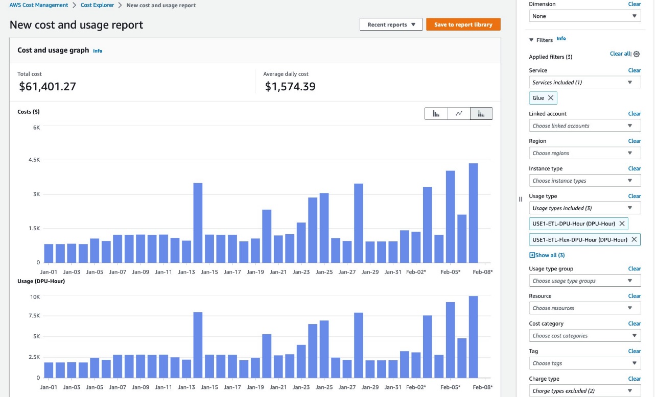


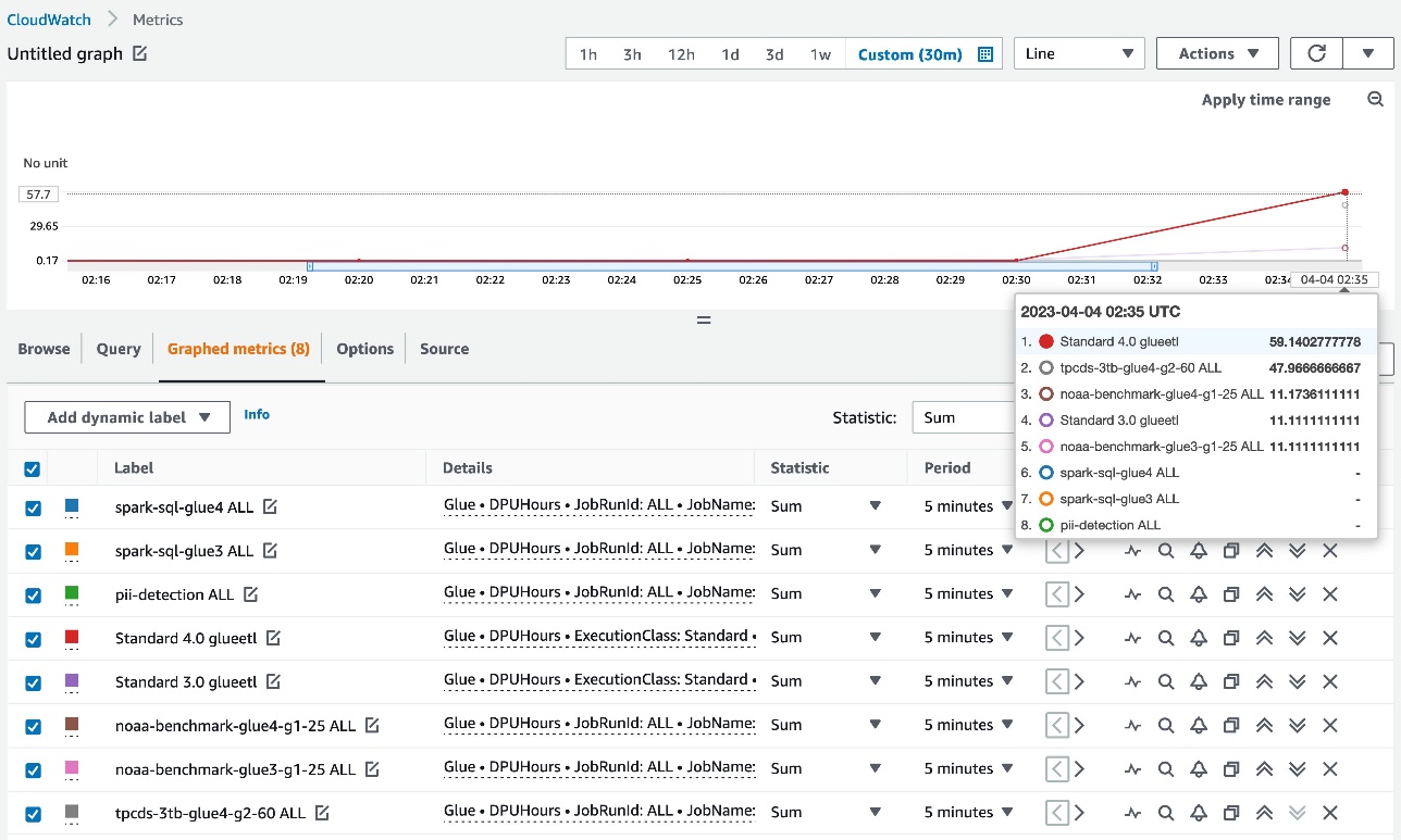



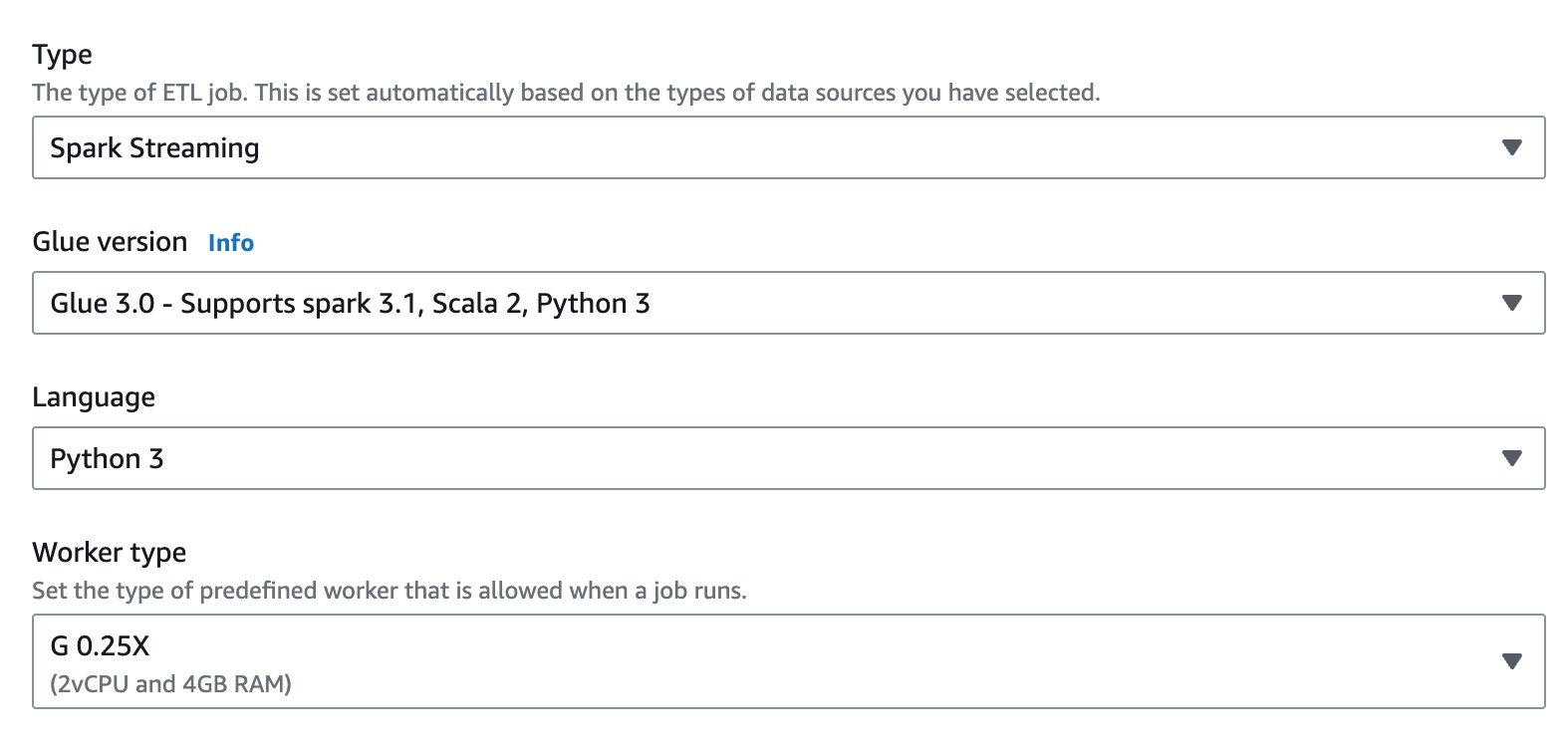

 Noritaka Sekiyama is a Principal Big Data Architect on the AWS Glue team. He is responsible for building software artifacts to help customers. In his spare time, he enjoys cycling with his new road bike.
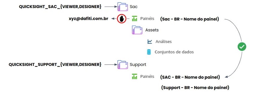
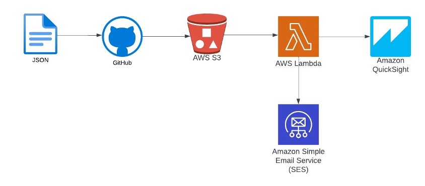
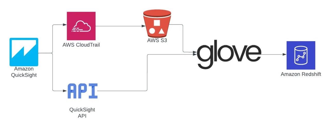
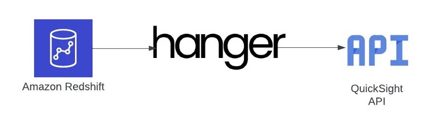
 Valdiney Gomes is Data Engineering Coordinator at Dafiti. He worked for many years in software engineering, migrated to data engineering, and currently leads an amazing team responsible for the data platform for Dafiti in Latin America.
 Hélio Leal is a Data Engineering Specialist at Dafiti, responsible for maintaining and evolving the entire data platform at Dafiti using AWS solutions.
 Flávia Lima is a Data Engineer at Dafiti, responsible for sustaining the data platform and providing the data from many sources to internal customers.


 Debaprasun Chakraborty is an AWS Solutions Architect, specializing in the analytics domain. He has around 20 years of software development and architecture experience. He is passionate about helping customers in cloud adoption, migration and strategy.
 Suraj Subramani Vineet is a Senior Cloud Architect at Amazon Web Services (AWS) Professional Services in Sydney, Australia. He specializes in designing and building scalable and cost-effective data platforms and AI/ML solutions in the cloud. Outside of work, he enjoys playing soccer on weekends.


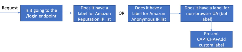
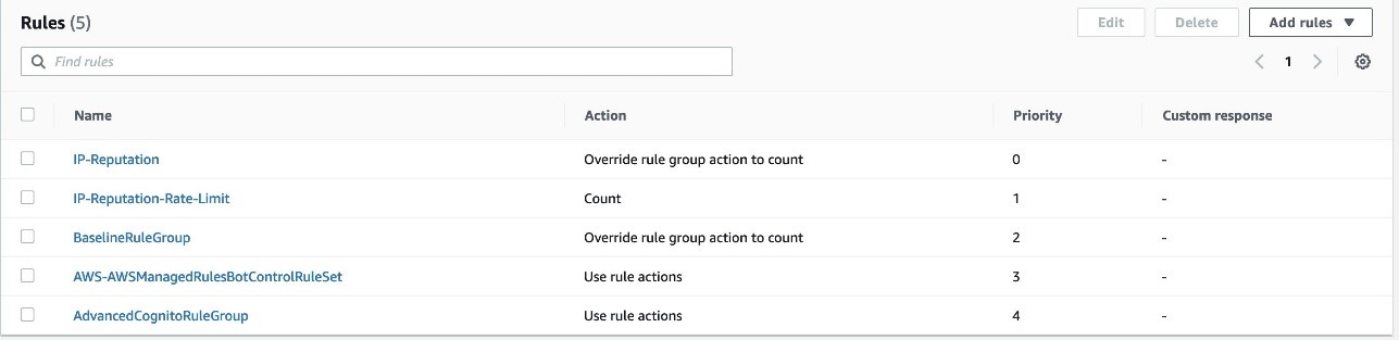


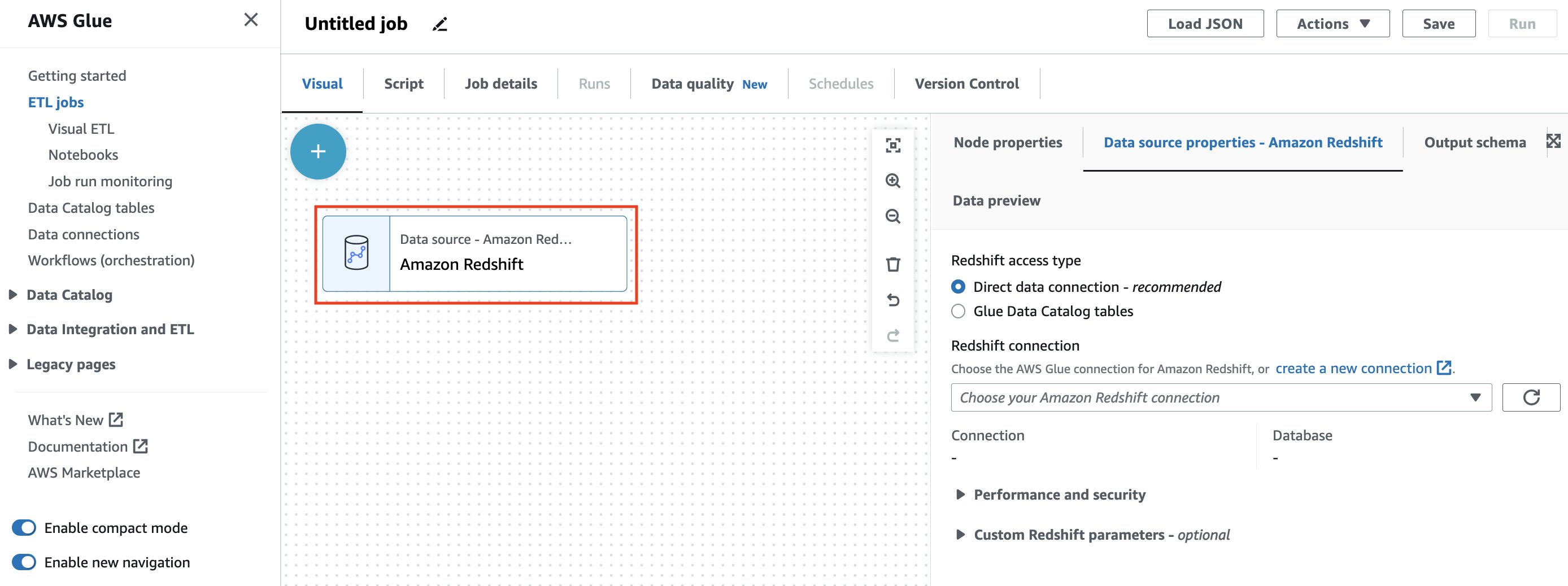


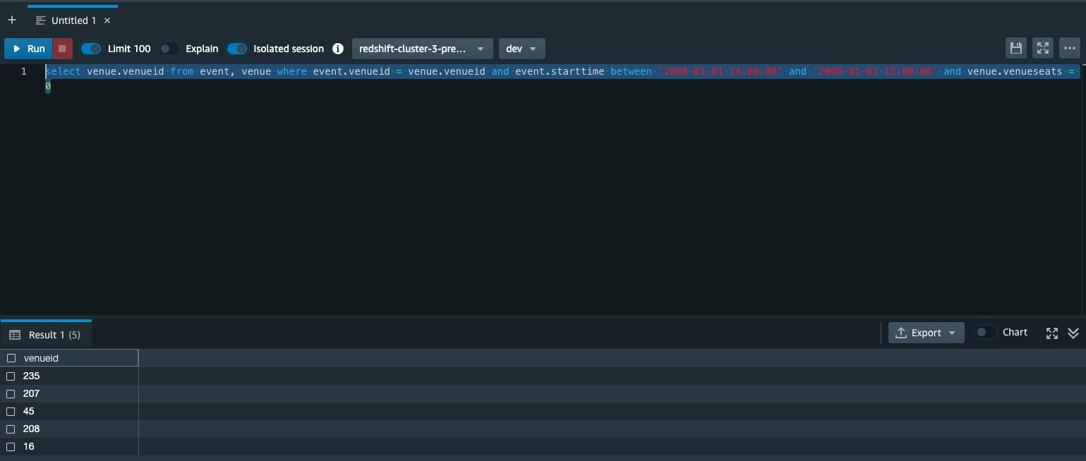


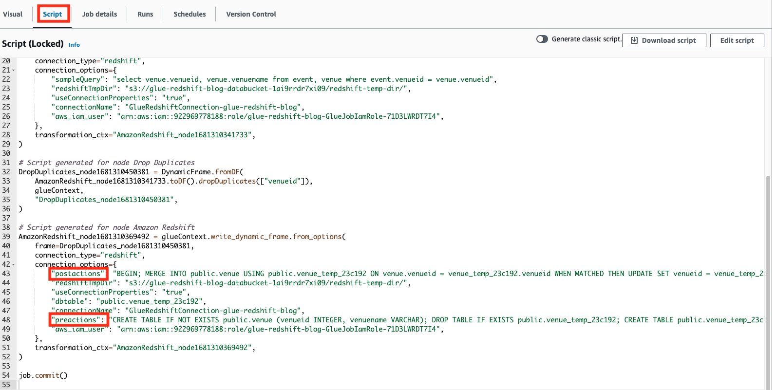
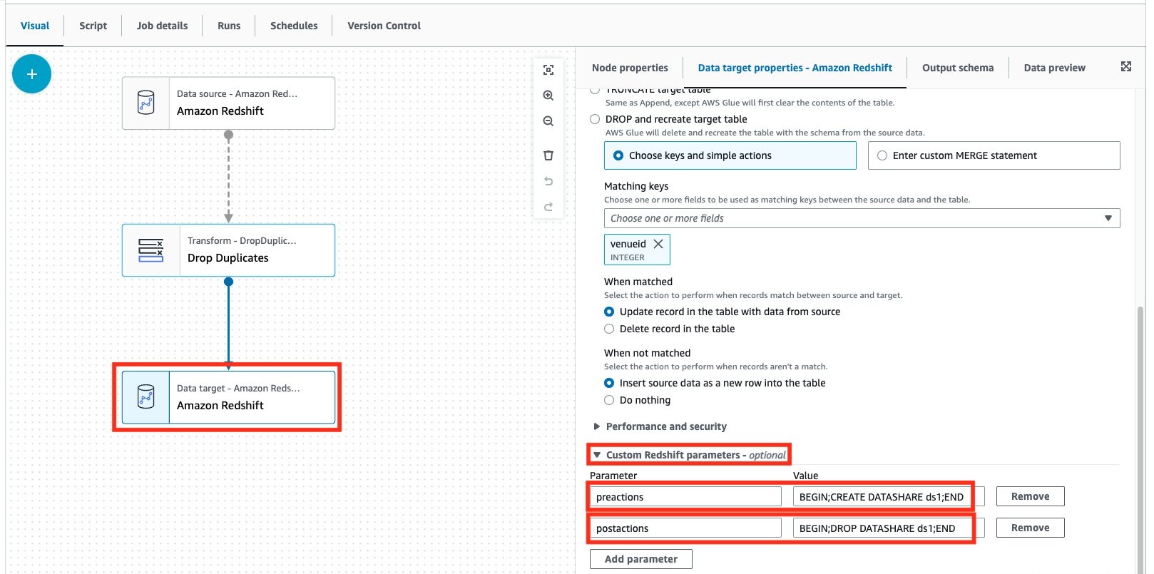
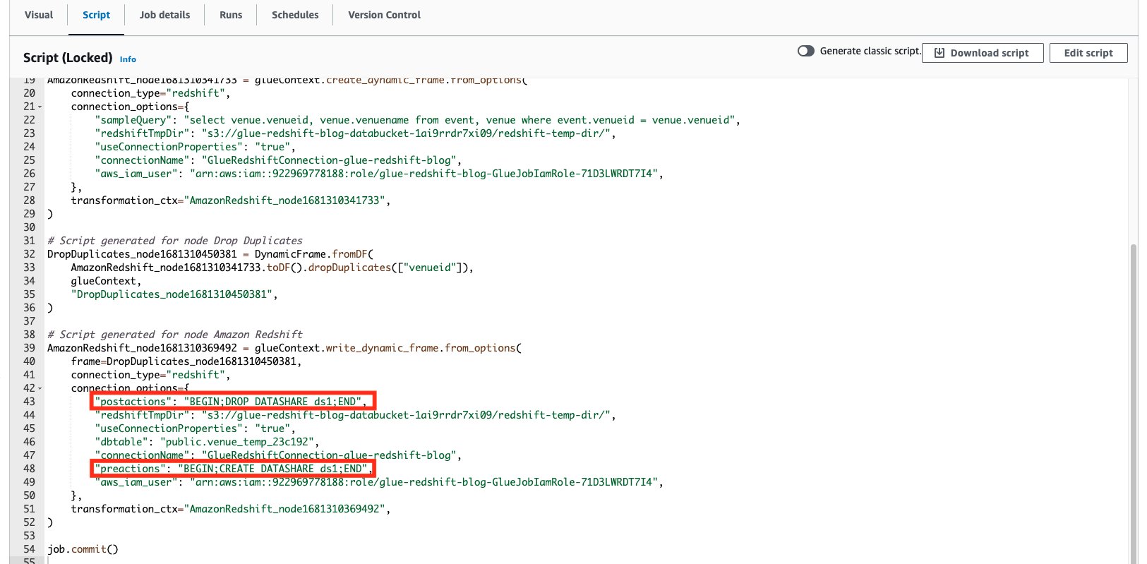
 Aniket Jiddigoudar is a Big Data Architect on the AWS Glue team. He works with customers to help improve their big data workloads. In his spare time, he enjoys trying out new food, playing video games, and kickboxing.
 Sean Ma is a Principal Product Manager on the AWS Glue team. He has an 18+ year track record of innovating and delivering enterprise products that unlock the power of data for users. Outside of work, Sean enjoys scuba diving and college football.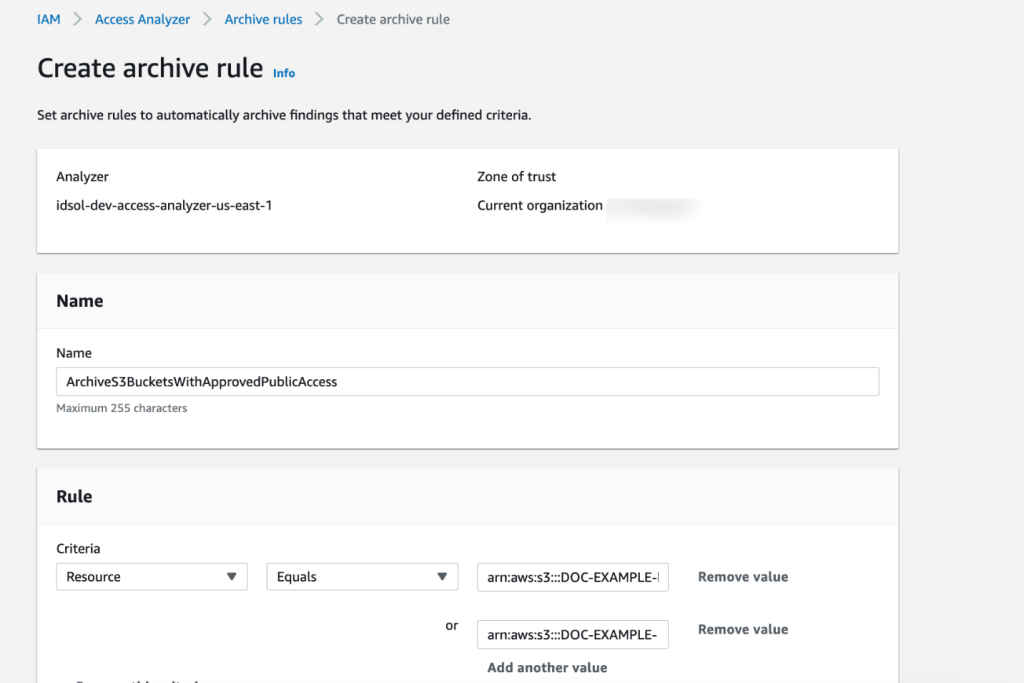

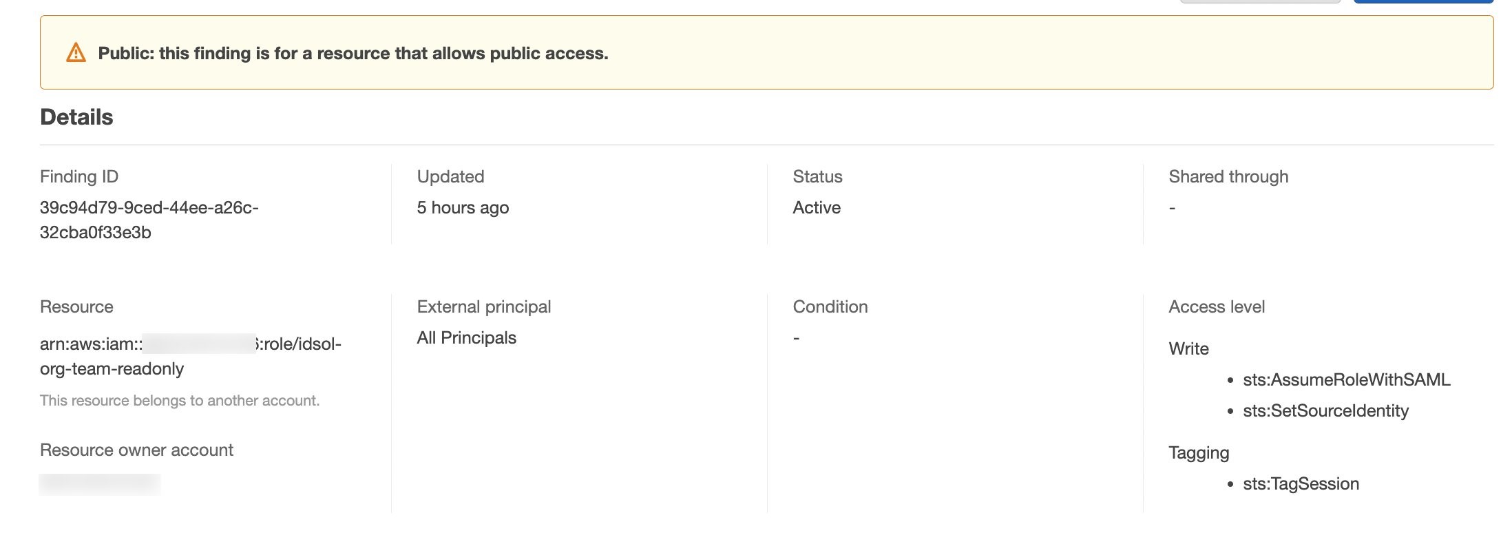
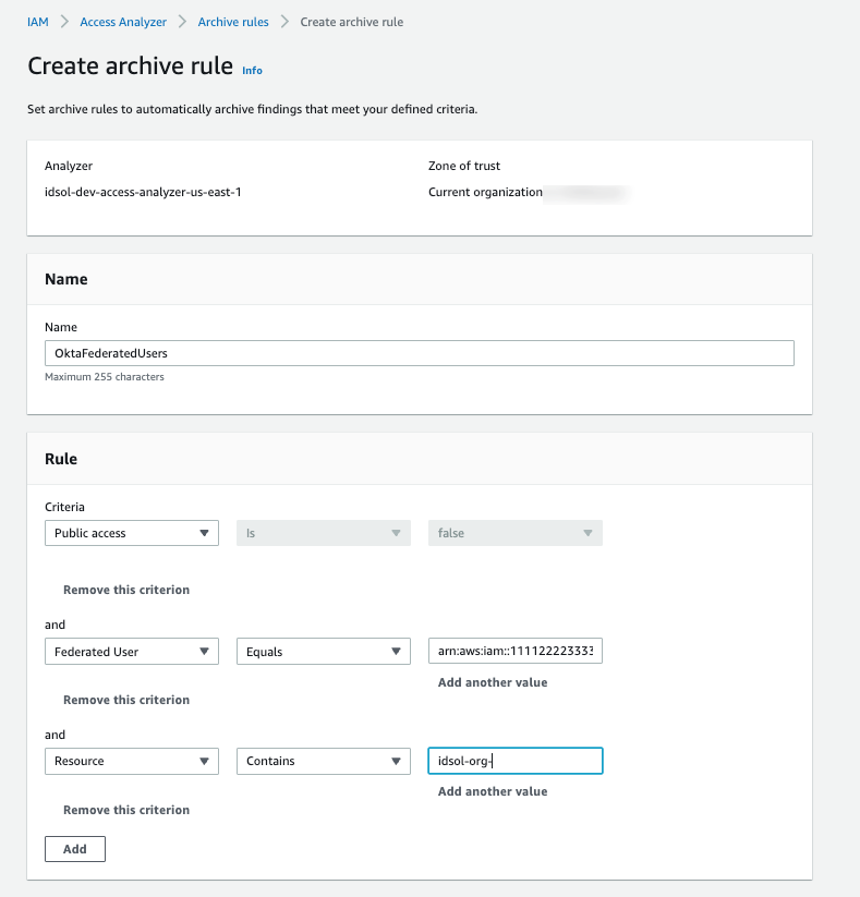
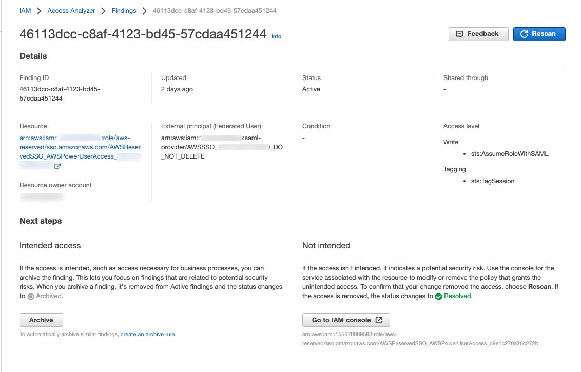
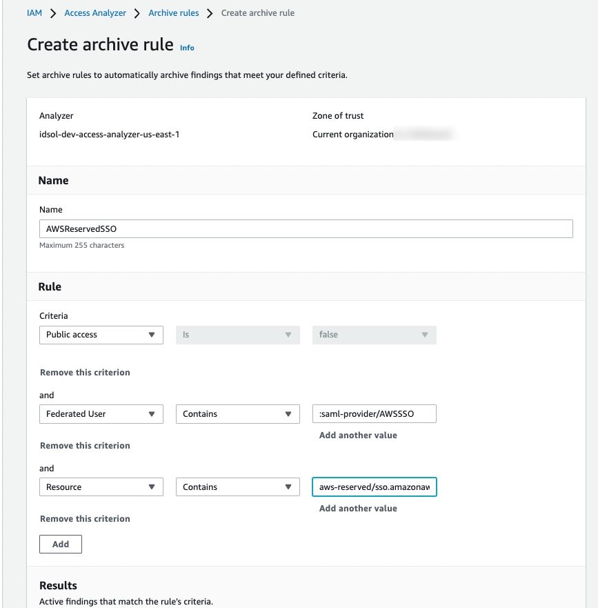
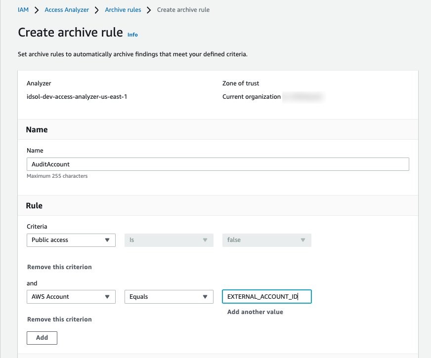


 Utkarsh Agarwal is a Cloud Support Engineer in the Support Engineering team at Amazon Web Services. He specializes in Amazon OpenSearch Service. He provides guidance and technical assistance to customers thus enabling them to build scalable, highly available and secure solutions in AWS Cloud. In his free time, he enjoys watching movies, TV series and of course cricket! Lately, he his also attempting to master the art of cooking in his free time – The taste buds are excited, but the kitchen might disagree.
 Ravi Bhatane is a software engineer with Amazon OpenSearch Serverless Service. He is passionate about security, distributed systems, and building scalable services. When he’s not coding, Ravi enjoys photography and exploring new hiking trails with his friends.
 Prashant Agrawal is a Sr. Search Specialist Solutions Architect with Amazon OpenSearch Service. He works closely with customers to help them migrate their workloads to the cloud and helps existing customers fine-tune their clusters to achieve better performance and save on cost. Before joining AWS, he helped various customers use OpenSearch and Elasticsearch for their search and log analytics use cases. When not working, you can find him traveling and exploring new places. In short, he likes doing Eat → Travel → Repeat.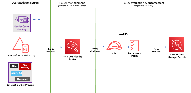
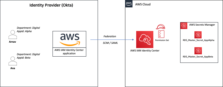


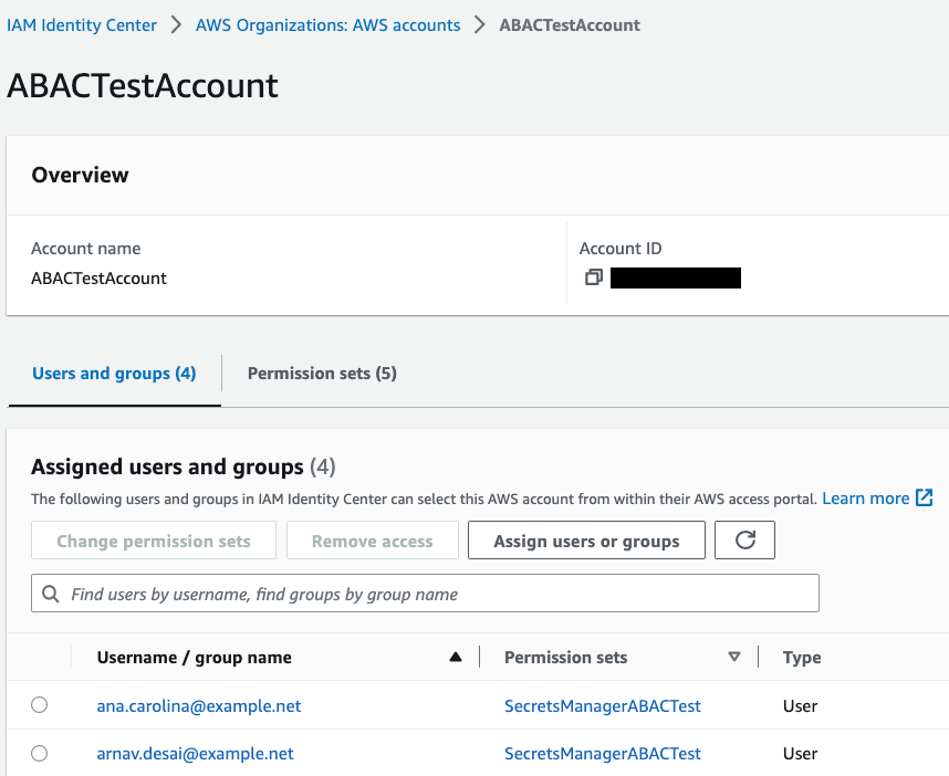


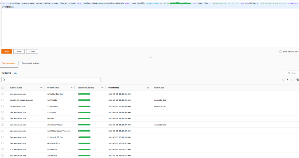
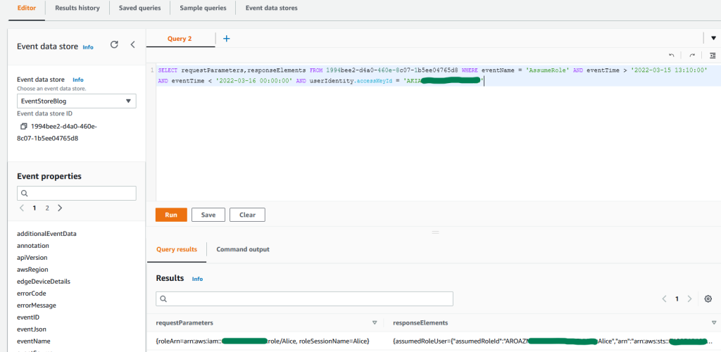
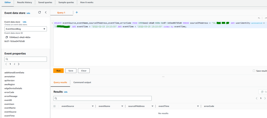
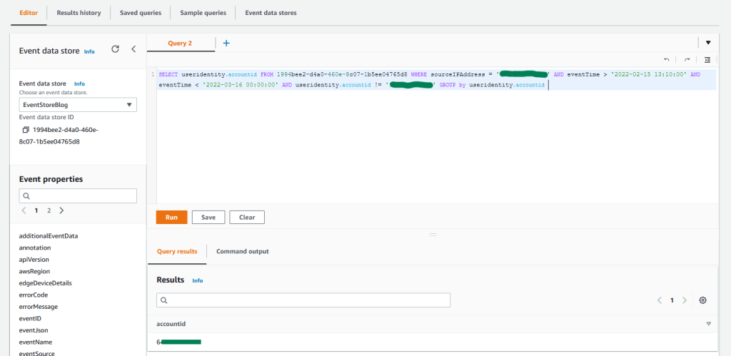
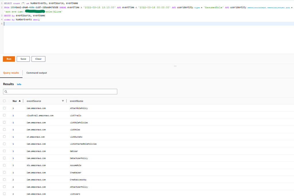
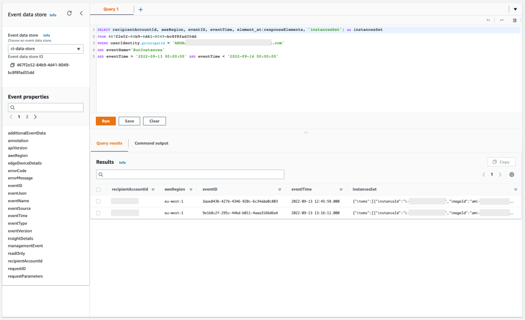
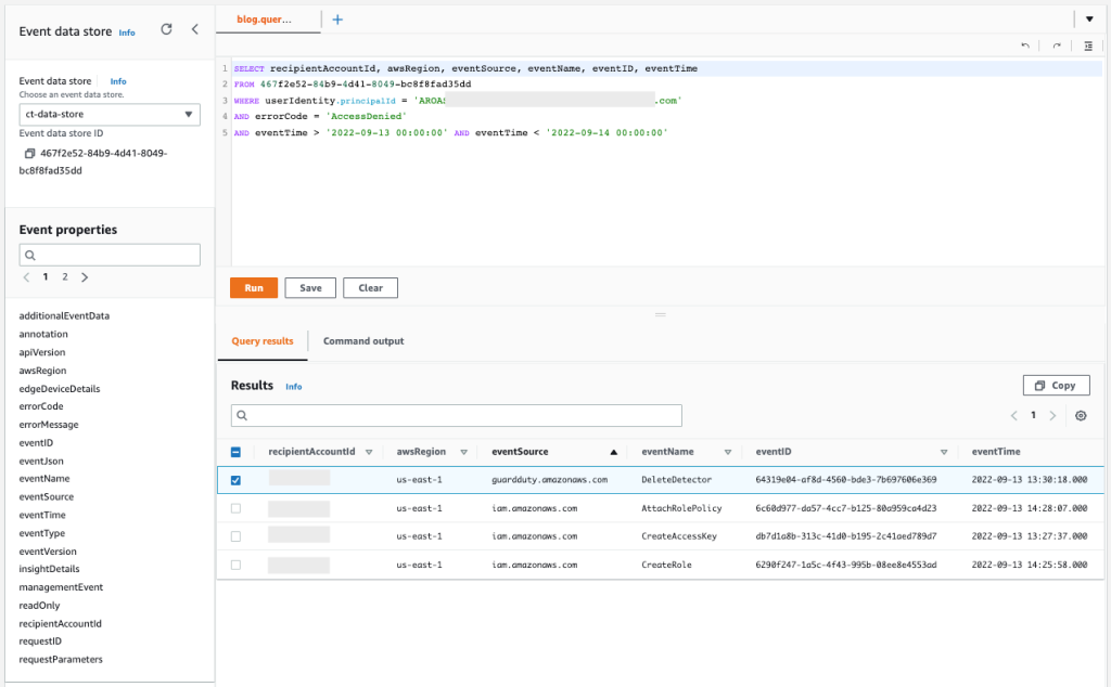
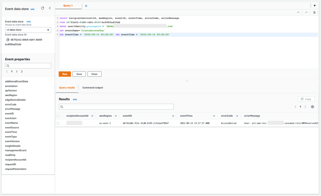
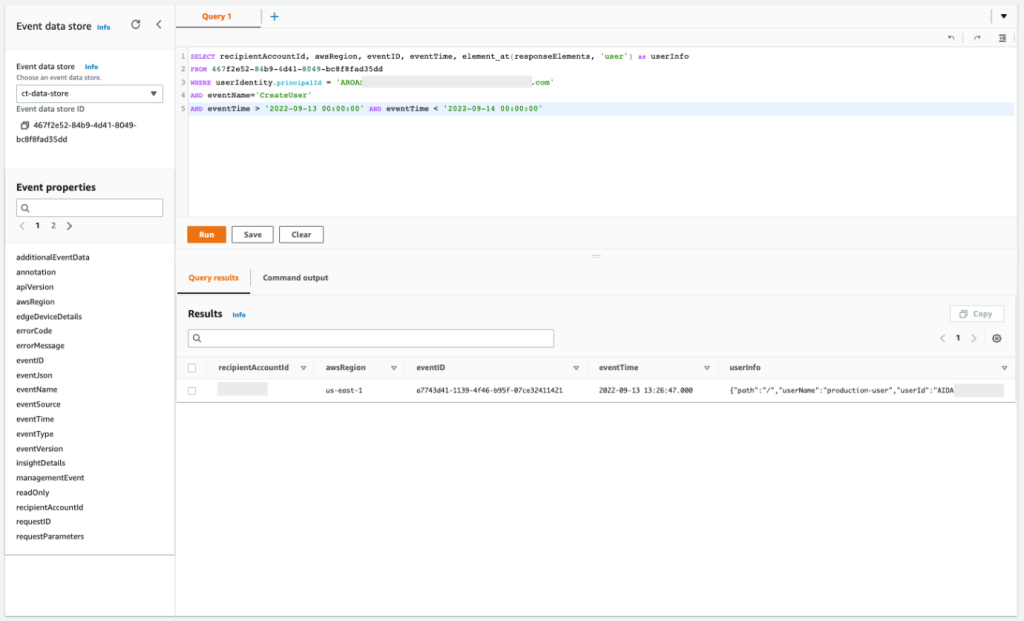
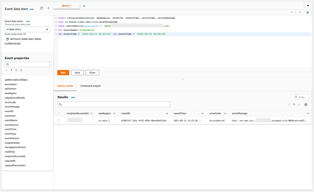
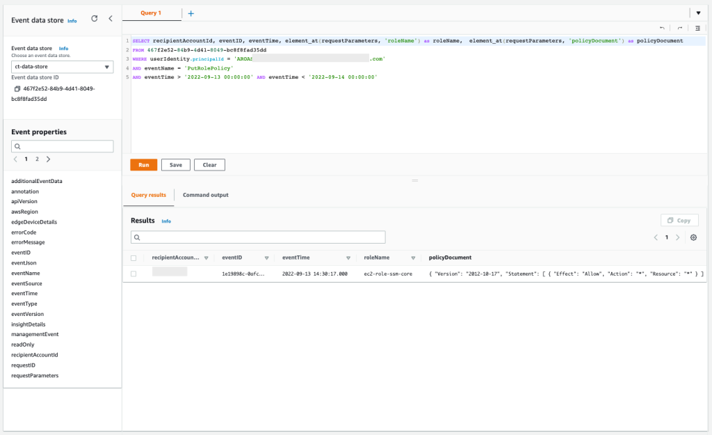


 Ennio Pastore is a Senior Data Architect on the AWS Data Lab team. He is an enthusiast of everything related to new technologies that have a positive impact on businesses and general livelihood. Ennio has over 10 years of experience in data analytics. He helps companies define and implement data platforms across industries, such as telecommunications, banking, gaming, retail, and insurance.
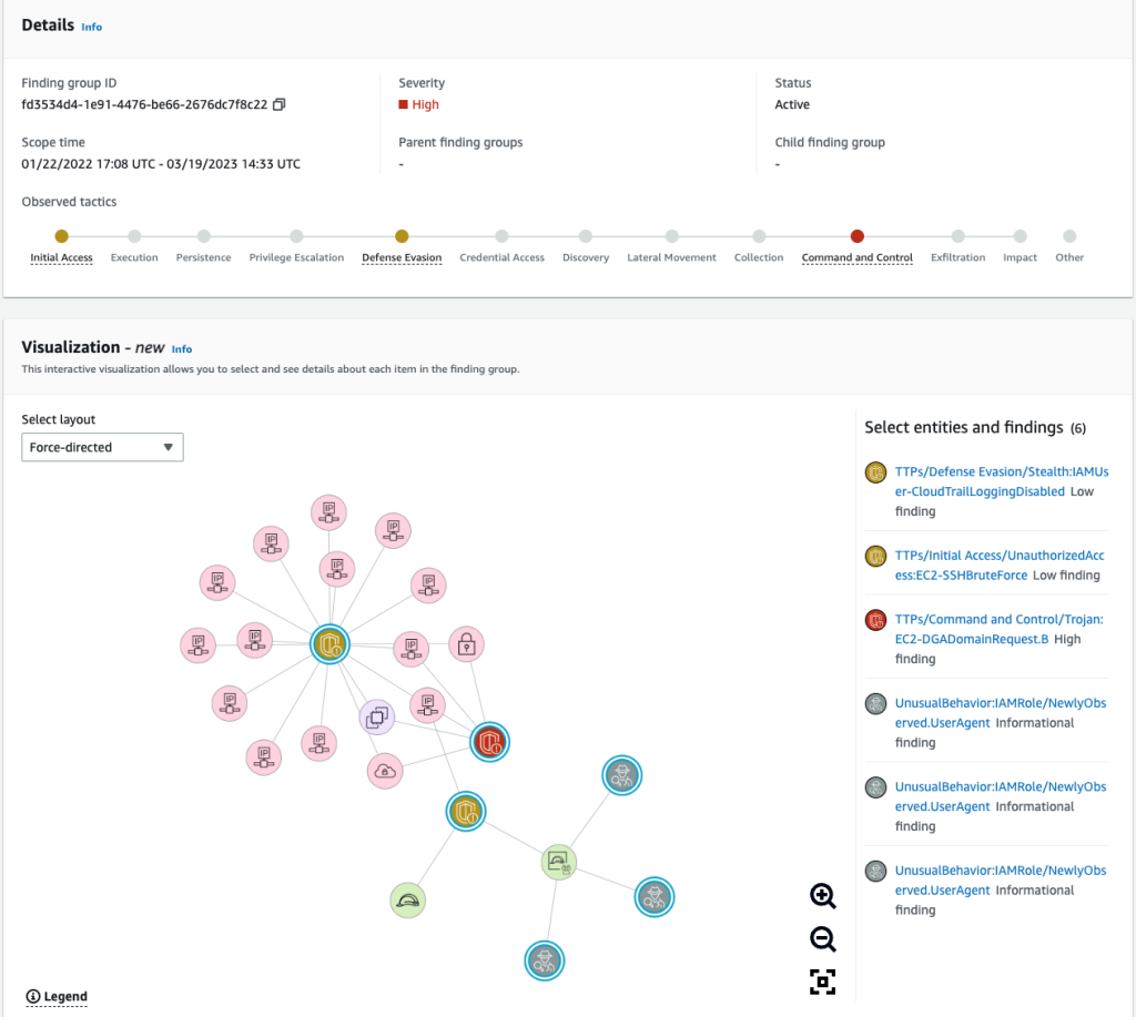

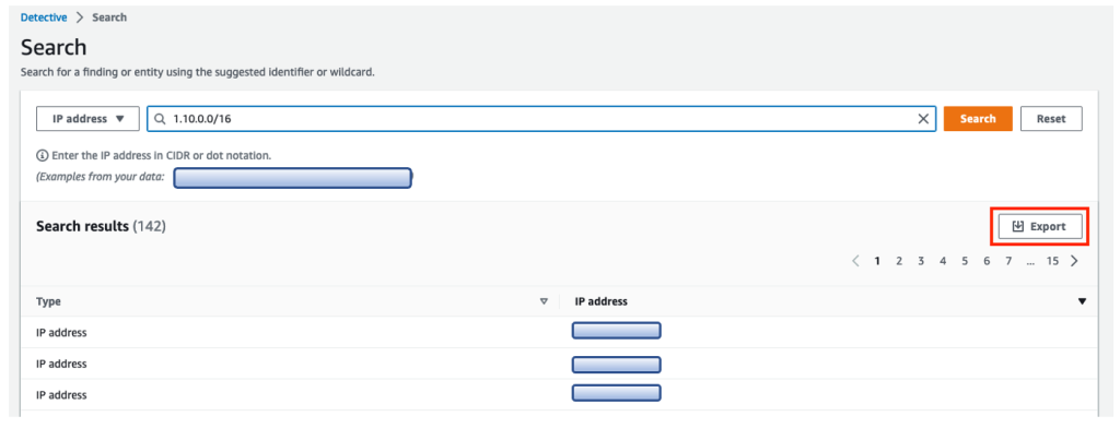


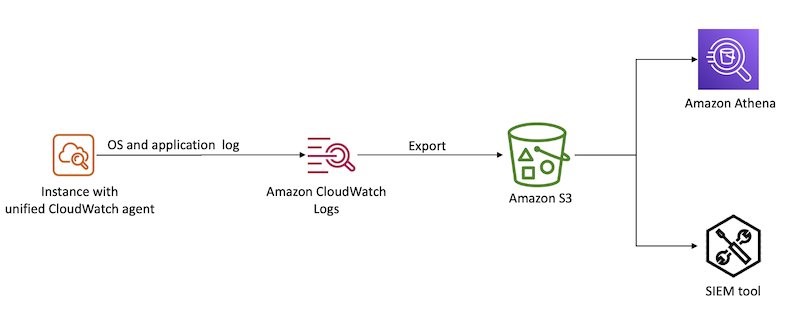
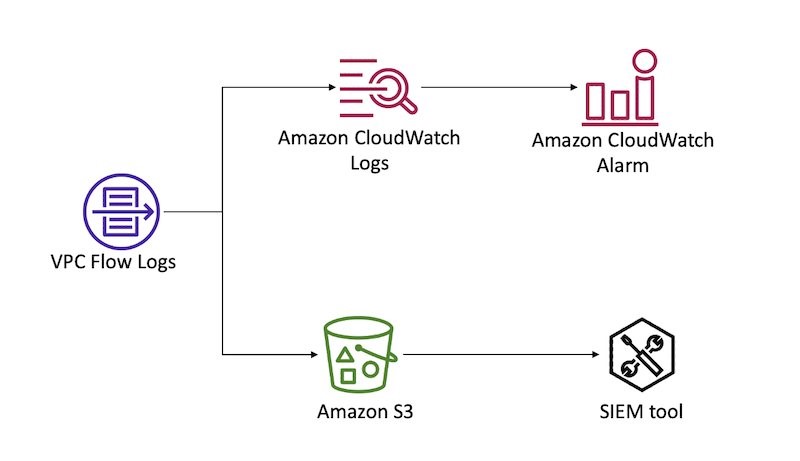
 Aruna Govindaraju is an Amazon OpenSearch Specialist Solutions Architect and has worked with many commercial and open-source search engines. She is passionate about search, relevancy, and user experience. Her expertise with correlating end-user signals with search engine behavior has helped many customers improve their search experience. Her favorite pastime is hiking the New England trails and mountains.

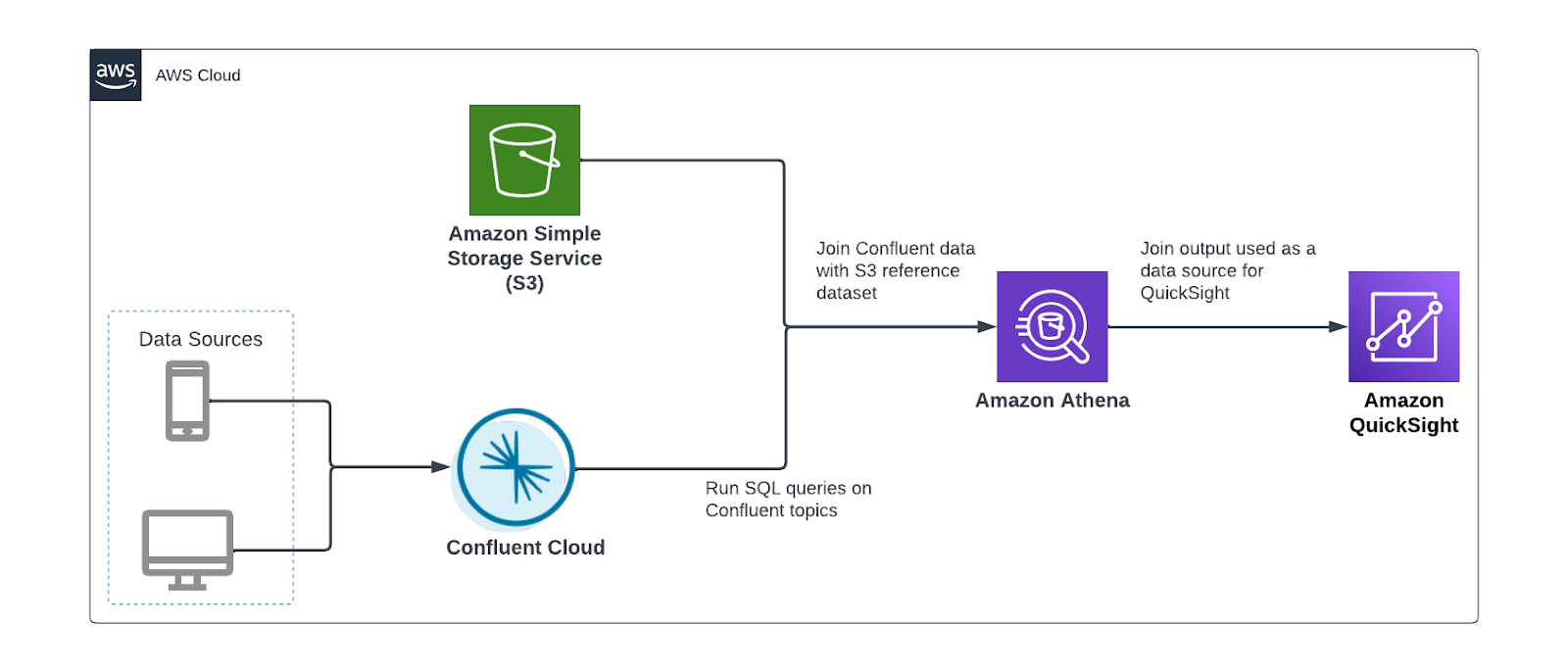


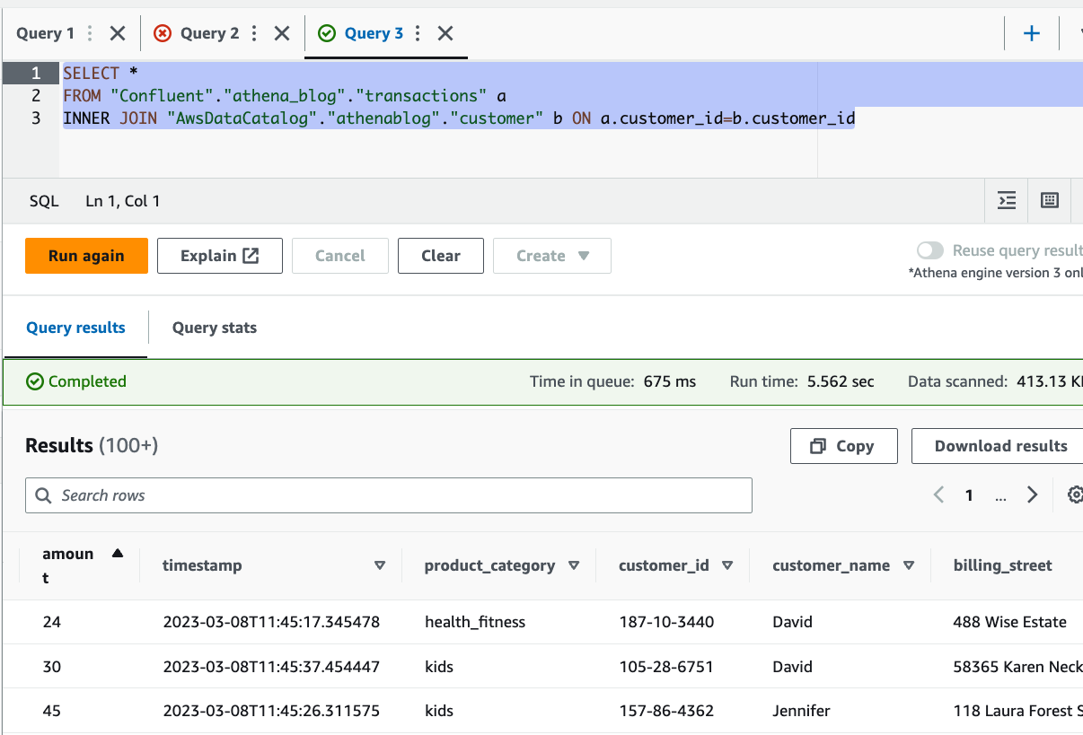


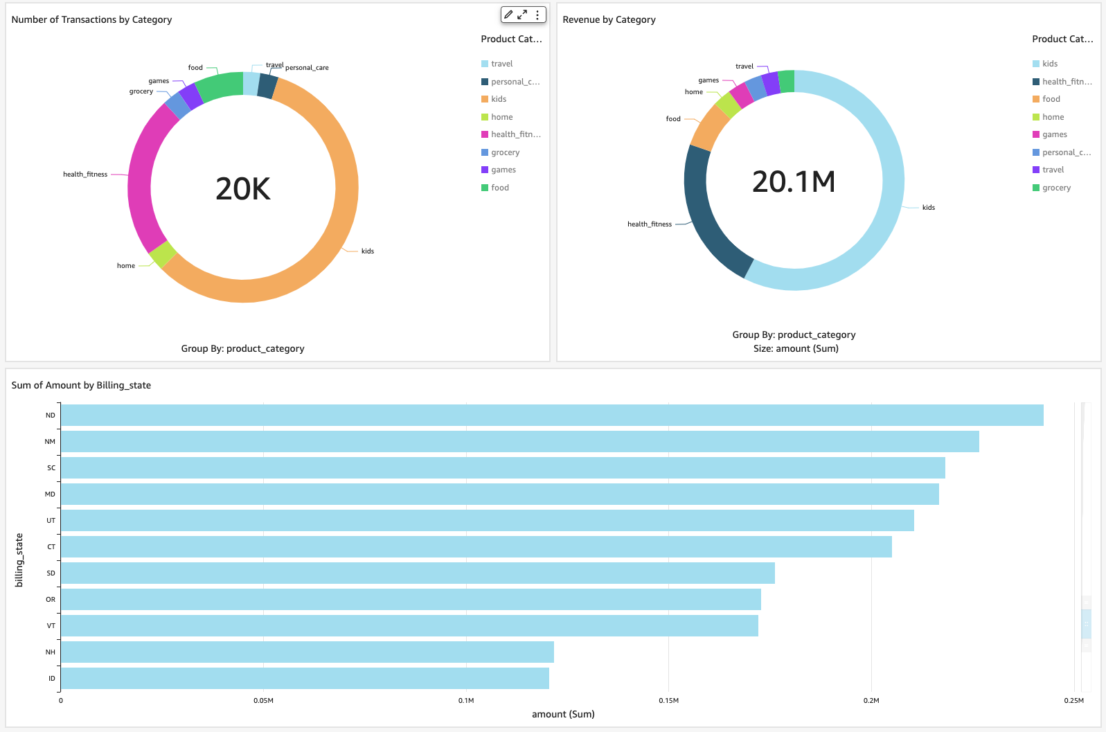
 Ahmed Zamzam is a Senior Partner Solutions Architect at Confluent, with a focus on the AWS partnership. In his role, he works with customers in the EMEA region across various industries to assist them in building applications that leverage their data using Confluent and AWS. Prior to Confluent, Ahmed was a Specialist Solutions Architect for Analytics AWS specialized in data streaming and search. In his free time, Ahmed enjoys traveling, playing tennis, and cycling.
 Geetha Anne is a Partner Solutions Engineer at Confluent with previous experience in implementing solutions for data-driven business problems on the cloud, involving data warehousing and real-time streaming analytics. She fell in love with distributed computing during her undergraduate days and has followed her interest ever since. Geetha provides technical guidance, design advice, and thought leadership to key Confluent customers and partners. She also enjoys teaching complex technical concepts to both tech-savvy and general audiences.


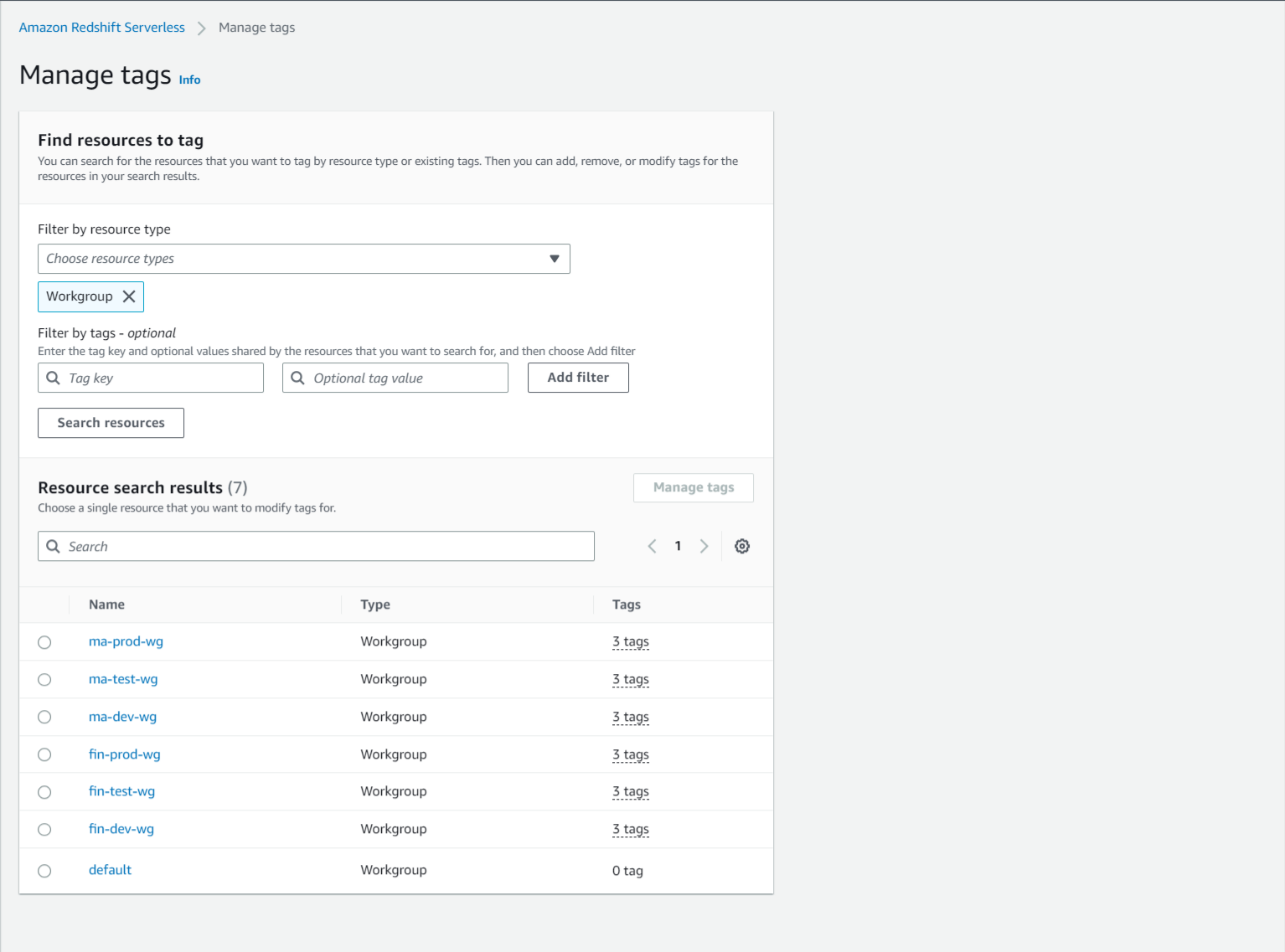

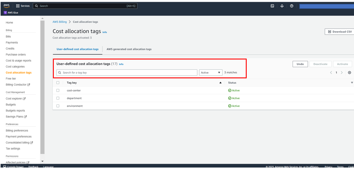


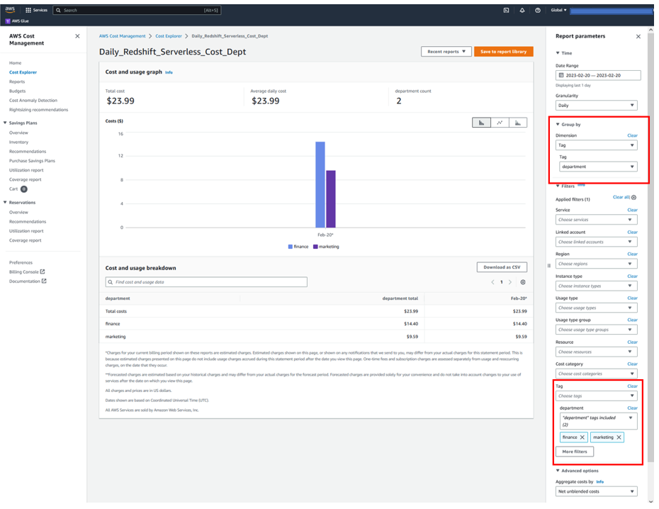
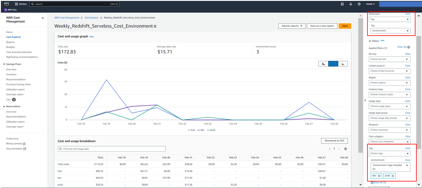
 Sandeep Bajwa is a Sr. Analytics Specialist based out of Northern Virginia, specialized in the design and implementation of analytics and data lake solutions.