Tag Archives: Intermediate (200)

How to monitor and query IAM resources at scale – Part 2

Post Syndicated from Michael Chan original https://aws.amazon.com/blogs/security/how-to-monitor-and-query-iam-resources-at-scale-part-2/

In this post, we continue with our recommendations for using AWS Identity and Access Management (IAM) APIs. In part 1 of this two-part series, we described how you could create IAM resources and use them soon after for authorization decisions. We also described options for monitoring and responding to IAM resource changes for entire accounts. Now, in part 2 of this post, we’ll cover the API throttling behavior of IAM and AWS Security Token Service (AWS STS) and how you can effectively plan your usage of these APIs. We’ll also cover the features of IAM that enable you to right-size the permissions granted to principals in your organization and assess external access to your resources.

Increase your usage of IAM APIs

If you’re a developer or a security engineer, you might find yourself writing more and more automation that interacts with IAM APIs. Other engineers, teams, or applications might also call the IAM APIs within the same account or cross-account. Over time, anyone calling the APIs in your account incrementally increases the number of requests per second. If so, IAM might send a “Rate exceeded” error that indicates you have exceeded a certain threshold of API calls per second. This is called API throttling.

Understand IAM API throttling

API throttling occurs when you exceed the call rate limits for an API. AWS uses API throttling to limit requests to a service. Like many AWS services, IAM limits API requests to maintain the performance of the service, and to ensure fair usage across customers. IAM and AWS STS independently implement a token bucket algorithm for throttling, in which a bucket of virtual tokens is refilled every second. Each token represents a non-throttled API call that you can make. The number of tokens that a bucket holds and the refill rate depends on the API. For each IAM API, a number of token buckets might apply.

We refer to this simply as rate-limiting criteria. Essentially, there are several rate-limiting criteria that are considered when evaluating whether a customer is generating more traffic than the service allows. The following are some examples of these criteria:

  • The account where the API is called
  • The account for read or write APIs (depending on whether the API is a read or write operation)
  • The account from which AssumeRole was called prior to the API call (for example, third-party cross-account calls)
  • The account from which AssumeRole was called prior to the API call for read APIs
  • The API and organization where the API is called

Understand STS API throttling

Although IAM has criteria pertaining to the account from which AssumeRole was called, IAM has its own API rate limits that are distinct from AWS STS. Therefore, the preceding criteria are IAM-specific and are separate from the throttling that can occur if you call STS APIs. IAM is also a global service, and the limits are not Region-aware. In contrast, while STS has a single global endpoint, every Region has its own STS endpoint with its own limits.

The STS rate-limiting criteria pertain to each account and endpoint for API calls. For example, if you call the AssumeRole API against the sts.ap-northeast-1.amazonaws.com endpoint, STS will evaluate the rate-limiting criteria associated with that account and the ap-northeast-1 endpoint. Other STS API requests that you perform under the same account and endpoint will also count towards these criteria. However, if you make a request from the same account to a different regional endpoint or the global endpoint, that request will count against different criteria.

Note: AWS recommends that you use the STS regional endpoints instead of the STS global endpoint. Regional endpoints have several benefits, including redundancy and reduced latency. To learn more about other benefits, see Managing AWS STS in an AWS Region.

How multiple criteria affect throttling

The preceding examples show the different ways that IAM and STS can independently limit requests. Limits might be applied at the account level and across read or write APIs. More than one rate-limiting criterion is typically associated with an API call, with each request counted against each rate-limiting criterion independently. This means that if the requests-per-second exceeds the applicable criteria, then API throttling occurs and returns a rate-limiting error.

How to address IAM and STS API throttling

In this section, we’ll walk you through some strategies to reduce IAM and STS API throttling.

Query for top callers

With AWS CloudTrail Lake, your organization can aggregate, store, and query events recorded by CloudTrail for auditing, security investigation, and operational troubleshooting. To monitor API throttling, you can run a simple query that identifies the top callers of IAM and STS.

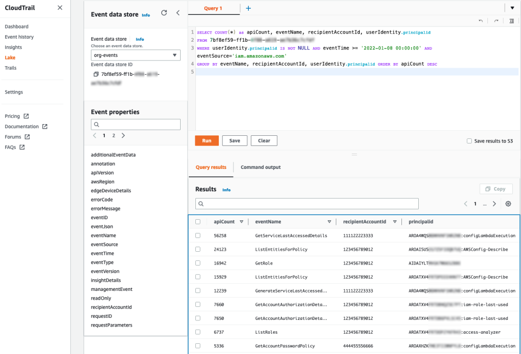
For example, you can make a SQL-based query in the CloudTrail console to identify the top callers of IAM, as shown in Figure 1. This query includes the API count, API event name, and more that are made to IAM (shown under eventSource). In this example, the top result is a call to GetServiceLastAccessedDetails, which occurred 163 times. The result includes the account ID and principal ID that made those requests.

Figure 1: Example AWS CloudTrail Lake query

Figure 1: Example AWS CloudTrail Lake query

You can enable AWS CloudTrail Lake for all accounts in your organization. For more information, see Announcing AWS CloudTrail Lake – a managed audit and security Lake. For sample queries, including top IAM actions by principal, see cloud-trail-lake-query-samples in our aws-samples GitHub repository.

Know when you exceed API call rate limits

To reduce call throttling, you need to know when you exceed a rate limit. You can identify when you are being throttled by catching the RateLimitExceeded exception in your API calls. Or, you can send your application logs to Amazon CloudWatch Logs and then configure a metric filter to record each time that throttling occurs, for later analysis or notification. Ideally, you should do this across your applications, and log this information centrally so that you can investigate whether calls from a specific account (such as your central monitoring account) are affecting API availability across your other accounts by exceeding a rate-limiting criterion in those accounts.

Call your APIs with a less aggressive retry strategy

In the AWS SDKs, you can use the existing retry library and provide a custom base for the initial sleep done between API calls. For example, you can set a custom configuration for the backoff or edit the defaults directly. The default SDK_DEFAULT_THROTTLED_BASE_DELAY is 500 milliseconds (ms) in the relevant Java SDK file, but if you’re experiencing throttling consistently, we recommend a minimum 1000 ms for the throttled base delay. You can change this value or implement a custom configuration through the PredefinedBackoffStrategies.SDKDefaultBackoffStrategy() class, which is referenced in the same file. As another example, in the Javascript SDK, you can edit the base retry of the retryDelayOptions configuration in the AWS.Config class, as described in the documentation.

The difference between making these changes and using the SDK defaults is that the custom base provides a less aggressive retry. You shouldn’t retry multiple requests that are throttled during the same one-second window. If the API has other applicable rate-limiting criteria, you can potentially exceed those limits as well, preventing other calls in your account from performing requests. Lastly, be careful that you don’t implement your own retry or backoff logic on top of the SDK retry or backoff logic because this could make throttling worse — instead, you should override the SDK defaults.

Reduce the number of requests by using max items

For some APIs, you can increase the number of items returned by a single API call. Consider the example of the GetServiceLastAccessedDetails API. This API returns a lot of data, but the results are truncated by default to 100 items, ordered alphabetically by the service namespace. If the number of items returned is greater than 100, then the results are paginated, and you need to make multiple requests to retrieve the paginated results individually. But if you increase the value of the MaxItems parameter, you can decrease the number of requests that you need to make to obtain paginated results.

AWS has hundreds of services, so you should set the value of the MaxItems parameter no higher than your application can handle (the response size could be large). At the time of our testing, the results were no longer truncated when this value was 300. For this particular API, IAM might return fewer results, even when more results are available. This means that your code still needs to check whether the results are paginated and make an additional request if paginated results are available.

Consistent use of the MaxItems parameter across AWS APIs can help reduce your total number of API requests. The MaxItems parameter is also available through the GetOrganizationsAccessReport operation, which defaults to 100 items but offers a maximum of 1000 items, with the same caveat that fewer results might be returned, so check for paginated results.

Smooth your high burst traffic

In the table from part 1 of this post, we stated that you should evaluate IAM resources every 24 hours. However, if you use a simple script to perform this check, you could initiate a throttling event. Consider the following fictional example:

As a member of ExampleCorp’s Security team, you are working on a task to evaluate the company’s IAM resources through some custom evaluation scripts. The scripts run in a central security account. ExampleCorp has 1000 accounts. You write automation that assumes a role in every account to run the GetAccountAuthorizationDetails API call. Everything works fine during development on a few accounts, but you later build a dashboard to graph the data. To get the results faster for the dashboard, you update your code to run concurrently every hour. But after this change, you notice that many requests result in the throttling error “Rate exceeded.” Other security teams see “Rate exceeded” errors in their application logs, too.

Can you guess what happened? When you tried to make the requests faster, you used concurrency to make the requests run in parallel. By initiating this large number of requests simultaneously, you exceeded the rate-limiting criteria for the security account from which the sts:AssumeRole action was called prior to the GetAccountAuthorizationDetails API call.

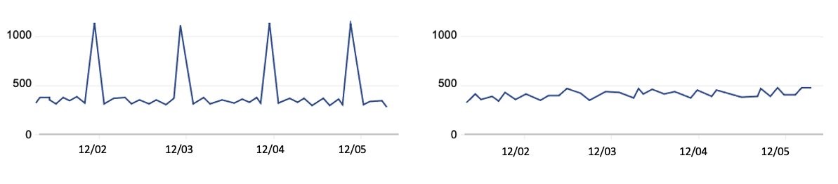
To address scenarios like this, we recommend that you set your own client-side limitations when you need to make a large number of API requests. You can spread these calls out so that they happen sequentially and avoid large spikes. For example, if you run checks every 24 hours, make sure that the calls don’t happen at exactly midnight. Figure 2 shows two different ways to distribute API volume over time:

Figure 2: Call volume that periodically spikes compared to evenly-distributed call volume

Figure 2: Call volume that periodically spikes compared to evenly-distributed call volume

The graph on the left represents a large, recurring API call volume, with calls occurring at roughly the same time each day—such as 1000 requests at midnight every 24 hours. However, if you intend to make these 1000 requests consistently every 24 hours, you can spread them out over the 24-hour period. This means that you could make about 41 requests every hour, so that 41 accounts are queried at 00:00 UTC, another 41 the next hour, and so on. By using this strategy, you can make these requests blend into your other traffic, as shown in the graph on the right, rather than create large spikes. In summary, your automation scheduler should avoid large spikes and distribute API requests evenly over the 24-hour period. Using queues such as those provided by Amazon Simple Queue Service (Amazon SQS) can also help, and when errors are identified, you can put them in a dead letter queue to try again later.

Some IAM APIs have rate-limiting criteria for API requests made from the account from which the AssumeRole was called prior to the call. We recommend that you serially iterate over the accounts in your organization to avoid throttling. To continue with our example, you should iterate the 41 accounts one-by-one each hour, rather than running 41 calls at once, to reduce spikes in your request rates.

Recommendations specific to STS

You can adjust how you use AWS STS to reduce your number of API calls. When you write code that calls the AssumeRole API, you can reuse the returned credentials for future requests because the credentials might still be valid. Imagine that you have an event-driven application running in a central account that assumes a role in a target account and does an API call for each event that occurs in that account. You should consider reusing the credentials returned by the AssumeRole call for each subsequent call in the target account, especially if calls in the central accounts are being throttled. You can do this for AssumeRole calls because there is no service-side limit to the number of credentials that you can create and use. Whether it’s one credential or many, you need to use and store these carefully. You can also adjust the role session duration, which determines how long the role’s credentials are valid. This value can be up to 12 hours, depending on the maximum session duration configured on the role. If you reuse short-term credentials or adjust the session duration, make sure that you evaluate these changes from a security perspective as you optimize your use of STS to reduce API call volume.

Use case #3: Pare down permissions for least-privileged access

Let’s assume that you want to evaluate your organization’s IAM resources with some custom evaluation scripts. AWS has native functionality that can reduce your need for a custom solution. Let’s take a look at some of these that can help you accomplish these goals.

Identify unintended external sharing

To identify whether resources in your accounts, such as IAM roles and S3 buckets, have been shared with external entities, you can use IAM Access Analyzer instead of writing your own checks. With IAM Access Analyzer, you can identify whether resources are accessible outside your account or even your entire organization. Not only can you identify these resources on-demand, but IAM Access Analyzer proactively re-analyzes resources when their policies change, and reports new findings. This can help you feel confident that you will be notified of new external sharing of supported resources, so that you can act quickly to investigate. For more details, see the IAM Access Analyzer user guide.

Right-size permissions

You can also use IAM Access Analyzer to help right-size the permissions policies for key roles in your accounts. IAM Access Analyzer has a policy generation feature that allows you to generate a policy by analyzing your CloudTrail logs to identify actions used from over 140 services. You can compare this generated policy with the existing policy to see if permissions are unused, and if so, remove them.

You can perform policy generation through the API or the IAM console. For example, you can use the console to navigate to the role that you want to analyze, and then choose Generate policy to start analyzing the actions used over a specified period. Actions that are missing from the generated policy are permissions that can be potentially removed from the existing policy, after you confirm your changes with those who administer the IAM role. To learn more about generating policies based on CloudTrail activity, see IAM Access Analyzer makes it easier to implement least privilege permissions by generating IAM policies based on access activity.

Conclusion

In this two-part series, you learned more about how to use IAM so that you can test and query IAM more efficiently. In this post, you learned about the rate-limiting criteria for IAM and STS, to help you address API throttling when increasing your usage of these services. You also learned how IAM Access Analyzer helps you identify unintended resource sharing while also generating policies that serve as a baseline for principals in your account. In part 1, you learned how to quickly create IAM resources and use them when refining permissions. You also learned how to get information about IAM resources and respond to IAM changes through the various services integrated with IAM. Lastly, when calling IAM directly, you learned about bulk APIs, which help you efficiently retrieve the state of your principals and policies. We hope these posts give you valuable insights about IAM to help you better monitor, review, and secure access to your AWS cloud environment!

If you have feedback about this post, submit comments in the Comments section below. If you have questions about this post, start a new thread on the Security, Identity, & Compliance re:Post or contact AWS Support.

Want more AWS Security news? Follow us on Twitter.

Michael Chan

Michael Chan

Michael is a Senior Solutions Architect for AWS Identity who has advised financial services and global customers of AWS. He enjoys understanding customer problems with identity and access management and helping them solve their security issues at scale.

Author photo

Joshua Du Lac

Josh is a Senior Manager of Security Solutions Architects at AWS. Based out of Texas, he has advised dozens of enterprise, global, and financial services customers to accelerate their journey to the cloud while improving their security along the way. Outside of work, Josh enjoys searching for the best tacos in Texas and practicing his handstands.

How to monitor and query IAM resources at scale – Part 1

Post Syndicated from Michael Chan original https://aws.amazon.com/blogs/security/how-to-monitor-and-query-iam-resources-at-scale-part-1/

In this two-part blog post, we’ll provide recommendations for using AWS Identity and Access Management (IAM) APIs, and we’ll share useful details on how IAM works so that you can use it more effectively. For example, you might be creating new IAM resources such as roles and policies through automation and notice a delay for resource propagations. Or you might be building a custom cloud security monitoring solution that uses IAM APIs to evaluate the security and compliance of your AWS accounts, and you want to know how to do that without exceeding limits. Although these are just a few example use cases, the insights described in this post are intended to help you avoid anti-patterns when building scalable cloud services that use IAM APIs.

In this post, we describe how to create IAM resources and use them soon after for authorization decisions. We also describe options for monitoring and responding to IAM resource changes for entire accounts. In part 2, we’ll cover the API throttling behavior of IAM and AWS Security Token Service (AWS STS) and how you can effectively plan your usage of these APIs. Let’s dive in!

Use case 1: Create IAM resources and attempt to use them immediately

If you’re a cloud developer, you create and use IAM resources when you develop applications on AWS. For your application to interact with AWS services, you need to grant IAM permissions to your application. Your application—whether it runs on AWS Lambda, Amazon Elastic Compute Cloud (Amazon EC2), or another service—will need an associated IAM role and policy that provide the necessary permissions.

Imagine that you want to create least privilege policies for your application. You begin by deploying new or updated IAM resources, such as roles and policies, along with your application updates, and you automate this process to speed up testing and development.

During development, you begin removing unnecessary policy permissions, with your automation testing the updated permissions. However, you notice that some of your updates do not immediately take effect. The following sections address why this occurs and provide insights to help you architect for other scenarios.

Understand the IAM control plane and data plane

Let’s first learn more about the control plane and data plane in IAM. The control plane involves operations to create, read, update, and delete IAM resources, and it’s how you get the current state of IAM. When you invoke IAM APIs, you interact with the control plane. This includes any API that falls under the iam:* namespace. The data plane, in contrast, consists of the authorization system that is used at scale to grant access to the broader set of AWS services and resources. This includes the AWS STS APIs, which have their own sts:* namespace.

When you call the IAM control plane APIs to create, update, or delete resources, you can expect a read-after-write consistent response. This means that you can retrieve (read) the resource and its latest updates immediately after it’s written. In contrast, the IAM data plane, where authorizations occur, is eventually consistent. This means that there will be a delay for IAM resource changes, such as updates to roles and policies, to propagate and reflect in the authorizations that follow. The delay can be several seconds or longer. Because of this, you need to allow for propagation time when you test changes to IAM resources. To learn more about the control plane and data plane of IAM, see Resilience in AWS Identity and Access Management.

Note: Because calls to AWS APIs rely on IAM to check permissions, the availability and scalability of the data plane are paramount. In 2011, the “can the caller do this?” function handled a couple of thousand requests per second. Today, as new services continue to launch and the number of AWS customers increases, AWS Identity handles over half a billion API calls per second worldwide, and the number is growing. Eventually consistent design enables the IAM data plane to maintain the high availability and low latency needed to evaluate permissions on AWS.

This is why when architecting your application, we recommend that you don’t depend on control plane actions such as resource updates for critical parts of your application’s workflow. Instead, you should architect to take advantage of the data plane, which includes STS and the authorization system of IAM. In the next section, we describe how you can do this.

Test permissions with STS scope-down policies

IAM role sessions have a feature called a session policy, which takes effect immediately when a role is assumed. This is an optional policy that you can provide to scope down the role’s existing identity policies, with the permissions being the intersection of the role’s identity-based policies and the session policy. By using session policies, you get specific, scoped-down credentials from a single pre-existing role without having to create new roles or identity policies for each particular session’s use case. You can use session policies for your application or when you test which least privilege policies are best for your application.

Let’s walk through an example of when to use session policies for permissions testing. Imagine that you need permissions that require very specific, fine-grained conditions to attain your ideal least privilege policy. You might iterate on the policy several times, making updates and testing the changes over and over again. If you update a policy attached to a role, you need to wait for these changes to propagate to the IAM data plane. But if you instead specify a scope-down policy when assuming the pre-existing role prior to testing, you can immediately test and observe the effects of your permissions changes. Immediate testing is possible because your role and its original policy have already propagated to the data plane, enabling you to iterate over various scoped-down session policies that operate against the IAM data plane.

Use STS session policies to assume a role with the AWS CLI

There are two ways to provide a session policy during the AssumeRole process: you can provide an inline policy document or the Amazon Resource Names (ARNs) of managed session policies. The following example shows how to do this through the AWS Command Line Interface (AWS CLI), by passing in a policy document along with the AssumeRole call. If you use this example policy, make sure to replace <123456789012> and <DOC-EXAMPLE-BUCKET> with your own information.

$ aws sts assume-role \
 --role-arn arn:aws:iam::<123456789012>:role/s3-full-access
 --role-session-name getobject-only-exco
 --policy '{ "Version": "2012-10-17", "Statement": [ { "Action": [ "s3:GetObject" ], "Effect": "Allow", "Resource": "arn:aws:s3::: <DOC-EXAMPLE-BUCKET>/*" } ] }'

In this example, we provide a previously created role ARN named s3-full-access, which provides full access to Amazon Simple Storage Service (Amazon S3). We can further restrict the role’s permissions by supplying a policy with the optional --policy option. The inline policy document only allows the GetObject request against the S3 bucket named <DOC-EXAMPLE-BUCKET>. The effective permissions for the returned session are the intersection of the role’s identity-based policies and our provided session policy. Therefore, the role session’s permissions are limited to only performing the GetObject request against the <DOC-EXAMPLE-BUCKET>.

Note: The combined size of the passed inline policy document and all passed managed policy ARN characters cannot exceed 2,048 characters. You can reduce the size of the JSON policy document by removing unnecessary whitespace and shortening or removing tags associated with your session.

To learn more about session permissions, see Create fine-grained session permissions using IAM managed policies. In part two of this post, we will describe how you can use role sessions when you need to provide credentials at a high rate.

Use case 2: Monitor and respond to IAM resources for entire accounts

You might need to periodically audit the state of your IAM resources, such as roles and policies, including whether these IAM resources have changed, in a single account or across your entire organization. For example, you might want to check whether roles have overly broad access to actions and resources. Or you might want to monitor IAM resource creation and updates to respond to security-relevant permission changes. In this section, you will learn how to choose the right tool for auditing and monitoring IAM resources across accounts. You will learn about the AWS services that support this use case, the benefits of polling compared to event-based architectures, and powerful APIs that aggregate common information.

Respond to configuration changes with an event-driven approach

Sometimes you might need to perform actions relatively quickly based on IAM changes. For example, you might need to check if a trust policy for a newly created or updated role allows cross-account access. In cases like this, you can use AWS Config rules, AWS CloudTrail, or Amazon EventBridge to detect state changes and perform actions based on these state changes. You can use AWS Config rules to evaluate whether a resource complies with the conditions that you specify. If it doesn’t comply, you can provide a workflow to remediate the non-compliance. With CloudTrail, you can monitor your account’s API calls, and log API calls for your accounts with AWS Organizations integration. EventBridge works closely with CloudTrail and helps you create rules that match incoming events and send them to targets, such as Lambda, where your code can perform analysis or automated remediation. You can even filter out events from your accounts and send them to a central account’s event bus for processing. For an example of how to use EventBridge with IAM Access Analyzer to remediate cross-account access in a role’s trust policy, see Automate resolution for IAM Access Analyzer cross-account access findings on IAM roles. Which feature you choose depends on whether you need to monitor one account or all accounts in your organization, as well as which solution you are more comfortable building with.

One caveat to an event-driven approach is that if many events occur over a short period and your application responds to each event with an IAM API call of its own, you could eventually be throttled by IAM. To address this, you can queue up your responding API calls, distribute them over a longer period, or aggregate them to reduce API call volume. For example, if some of your calls are write APIs (such as UpdateAssumeRolePolicy or CreatePolicyVersion) or read APIs (such as GetRole or GetRolePolicy), you can call them serially with a delay between calls. If you need the latest status on a large number of principals and policies, you can call IAM bulk APIs such as GetAccountAuthorizationDetails, which will return data to you for principals and policies and their relationships in your organization. This approach helps you avoid throttling and querying the IAM control plane with unnecessary and redundant API calls. You will learn more about throttling and how to address it in part two of this post.

Retrieve point-in-time resource information with AWS Config

AWS Config helps you assess, audit, and evaluate the configuration of your AWS resources. It also offers multi-account, multi-Region data aggregation and is integrated with AWS Organizations. With AWS Config, you can create rules that detect and respond to changes. AWS Config also keeps an inventory of AWS resource configurations that you can query through its API, so that you don’t need to make direct API calls to each resource’s service. AWS Config also offers the ability to return the status of resources from multiple accounts and AWS Regions. As shown in Figure 1, you can use the AWS Config console to run a simple SQL-like statement for details on the IAM roles in your entire organization.

Figure 1: Run a query on IAM roles in AWS Config

Figure 1: Run a query on IAM roles in AWS Config

The preceding results also show associated resources, such as the inline and attached policies for the IAM roles. Alternatively, you can obtain these results from the SDK or CLI. The following query that uses the CLI is equivalent to the preceding query that uses the console. If you use this query, make sure to replace DOC-EXAMPLE-CONFIG-AGGREGATOR> with your AWS Config aggregator.

aws configservice select-aggregate-resource-config
--configuration-aggregator-name <DOC-EXAMPLE-CONFIG-AGGREGATOR>
--expression "SELECT accountId, resourceId, resourceName, resourceType, tags, configuration.attachedManagedPolicies, configuration.rolePolicyList WHERE resourceType = 'AWS::IAM::Role'"

Here is the response (note that we’ve adjusted the formatting to make it more readable):

{
  "accountId": "123456789012",
  "resourceId": "AROAI3X5HCEQIIEXAMPLE",
  "configuration": { 
    "attachedManagedPolicies": [
      {     
        "policyArn": "arn:aws:iam::aws:policy/service-role/AWSLambdaBasicExecutionRole",
        "policyName": "AWSLambdaBasicExecutionRole"
      },    
      {     
        "policyArn": "arn:aws:iam::123456789012:policy/mchan-test-cloudtrail-post-to-SNS",
        "policyName": "mchan-test-cloudtrail-post-to-SNS"
      }     
      ],    
    "rolePolicyList": []
  },
  "resourceName": "lambda-cloudtrail-notifications",
  "tags": [],
  "resourceType": "AWS::IAM::Role"
}

The preceding command returns the details of roles in your organization’s accounts, including the full policy document for the associated inline policy. It also returns the customer-managed policy names and their ARNs, for which you can view the policy documents and versions by using the BatchGetResourceConfig API. Note that AWS Config doesn’t provide the AWS-managed policy documents. However, these are common across accounts, and we will show you how to query that data later in this section.

To query the status of roles in your organization, you need to have AWS Config enabled in each account. You also need an aggregator to monitor your accounts with your organization’s management account or a delegated administrator account. For more details on how to set up AWS Config, see the AWS Config developer guide. After you set up AWS Config, you can periodically call the AWS Config APIs to get a snapshot of the current or prior state of your resources. Furthermore, you can periodically pull the snapshot records and evaluate this information in other tools outside of AWS Config. So before you directly use the IAM APIs to get IAM information, consider using AWS Config—this is what it’s for!

Retrieve IAM resource information directly from IAM

As previously noted, AWS Config can give you a bulk view of your AWS and IAM resources. Additionally, CloudTrail and EventBridge can detect AWS and IAM resource changes and help you act on them. If you need data from IAM beyond what these services offer, you can query the IAM APIs directly to get the latest information on your resources.

A few key APIs can help you audit IAM resources more efficiently, especially in bulk. The first is GetAccountAuthorizationDetails, which enables you to retrieve the principals in your account, their associated inline policy documents (if any), attached managed policies, and their relationships to each other. This API reduces the need to individually call ListRolePolicies and ListAttachedRolePolicies for each role in an account. GetAccountAuthorizationDetails also returns the role trust policy document for roles in the results. Finally, GetAccountAuthorizationDetails allows you to filter the result set. For example, if you don’t need information relating to groups or AWS managed policies, you can exclude these from the API response. You can do this by using the filter parameter to only include the details that you need at the time.

Another useful API is GenerateServiceLastAccessedDetails. This API gives you details about when an IAM resource (user, group, role, or policy) was last used in an attempt to access AWS services. You can use this API to identify roles that are unused and remove them if you don’t need them. IAM Access Analyzer, which you will learn about later in this post, also uses the same information.

The following table summarizes the key APIs that you can use, rather than building your own code that loops for this information individually.

Type of information API How to use the API Frequency of use
User list and user detail GetAccountAuthorizationDetails Pass User to the filter parameter When needed, per account
User’s inline policy User’s inline policy GetAccountAuthorizationDetails Pass User to the filter parameter When needed, per account
User’s attached managed policies GetAccountAuthorizationDetails Pass User to the filter parameter When needed, per account
Role list and role detail GetAccountAuthorizationDetails Pass Role to the filter parameter When needed, per account
Role trust policy GetAccountAuthorizationDetails Pass Role to the filter parameter When needed, per account
Role’s inline policy GetAccountAuthorizationDetails Pass Role to the filter parameter When needed, per account
Role’s attached managed policies GetAccountAuthorizationDetails Pass Role to the filter parameter When needed, per account
Role last used GetAccountAuthorizationDetails Pass Role to the filter parameter When needed, per account
Group list and group detail GetAccountAuthorizationDetails Pass Group to the filter parameter When needed, per account
Group’s inline policy GetAccountAuthorizationDetails Pass Group to the filter parameter When needed, per account
Group’s attached managed policies GetAccountAuthorizationDetails Pass Group to the filter parameter When needed, per account
AWS customer managed policies GetAccountAuthorizationDetails Pass LocalManagedPolicy to the filter parameter When needed, per account
AWS managed policies GetAccountAuthorizationDetails Pass LocalManagedPolicy to the filter parameter 24 hours recommended, globally (once for all accounts within an AWS partition)
Policy versions GetAccountAuthorizationDetails Pass either LocalManagedPolicy or WSManagedPolicy to the filter parameter 24 hours recommended, per account
Services access attempts by an IAM resource GetServiceLastAccessedDetails Submit a job through the GenerateServiceLastAccessedDetails API, which returns a JobId; then retrieve the results after the job completes. Spread total number of requests evenly across 24 hours
Actions access attempts by an IAM resource GetServiceLastAccessedDetails Submit a job through the GenerateServiceLastAccessedDetails API which returns a JobId; then retrieve the results after the job completes. Pass ACTION_LEVEL as the required Granularity parameter. Spread total number of requests evenly across 24 hours

Note: In the table, we suggest that you perform some of these API requests once every 24 hours as a starting point. You might prefer to perform your own analysis at a longer time interval, such as every 48 hours, but we don’t recommend requesting it more often than every 24 hours because these resources (and therefore the details in the responses) don’t change often. These APIs are suitable for periodic, point-in-time collection of information. If you need faster detection of information from GetAccountAuthorizationDetails, consider whether AWS Config rules or EventBridge will fit your needs. For GetServiceLastAccessedDetails, recent activity usually appears within four hours, so more frequent requests are unlikely to provide much value.

Use of these APIs can help you avoid writing code that loops through results to make individual read API calls for each principal, policy, and policy version in an account, which could result in tens of thousands of API requests and call throttling. Instead of iterating over each resource, you should use solutions that return bulk data, such as GetAccountAuthorizationDetails, AWS Config, or an AWS Partner Network solution. However, if you’re experiencing throttling, you will learn some practical considerations on how to handle that later in this post.

Inspect IAM resources across multiple accounts and organizations

Your use case might require that you inspect IAM resources across multiple accounts in your organization. Or perhaps you are an independent software vendor and need to build a software-as-a-service tool to evaluate IAM resources across many organizations. The following considerations can help you address use cases like these.

AWS Organizations integration

Previously, you learned of the benefits of the “service last accessed data” that the GenerateServiceLastAccessedDetails and GetServiceLastAccessedDetails APIs provide. But what if you want to pull this data for multiple accounts in your organization? IAM has bulk APIs that support querying this data across your entire organization, so you don’t need to assume a role in each account to generate the request. To generate a report for entities (organization root, organizational unit, or account) or policies in your organization, use the GenerateOrganizationsAccessReport operation, which returns a JobId that is passed as a parameter to the GetOrganizationsAccessReport operation to check if the report has been generated. When the job status is marked complete, you can retrieve the report.

AWS managed policies

Many customers use AWS managed policies because they align to common job functions. AWS creates and administers these policies, which have their own ARNs, such as arn:aws:iam::aws:policy/AWSCodeCommitPowerUser. AWS managed policies are available for every account, and they are the same for every account. AWS updates them when new services and API operations are introduced. Updated policies are recorded and visible as a new version, so you only need to query for the current AWS managed policies once per evaluation cycle, rather than once per account. Therefore, if you’re evaluating hundreds or thousands of accounts, you shouldn’t include the AWS managed policies and their policy versions in your query. Doing so would result in thousands of redundant API requests and could cause throttling. Instead, you can query the AWS managed policies once and then reuse the results across your analysis and evaluation by caching the results for a period of time (for example, every 24 hours) in your application before requesting them again to check for updates. Because AWS managed policies are available through the GetAccountAuthorizationDetails API, you don’t need to query for the AWS managed policies or their versions as a separate action.

Multi-account limits

The preceding table lists the frequency of API requests as “per account” in many places. If you’re calling IAM APIs by assuming a role in other accounts from a central account, some IAM APIs have rate-limiting criteria that apply to API requests performed from the assuming account (the central account). To query data from multiple accounts, we recommend that you serially iterate over the accounts one-by-one to avoid throttling. You’ll learn more about this strategy, as well as throttling, in part 2 of this blog post.

Conclusion

In this post, you learned about different aspects of IAM and best practices to test and query IAM efficiently. With STS session policies, you can test different policies to help achieve least privilege access. With AWS Config, EventBridge, CloudTrail, and CloudTrail Lake, you can audit your IAM resources and respond to changes while reducing the number of IAM API calls that you make. If you need to call IAM directly, you can use IAM bulk APIs for more efficient retrieval of your resource state. You can learn more about IAM and best practices in part 2 of blog post: How to monitor and query IAM resources at scale – Part 2.

If you have feedback about this post, submit comments in the Comments section below. If you have questions about this post, start a new thread on the Security, Identity, & Compliance re:Post or contact AWS Support.

Want more AWS Security news? Follow us on Twitter.

Michael Chan

Michael Chan

Michael is a Senior Solutions Architect for AWS Identity who has advised financial services and global customers of AWS. He enjoys understanding customer problems with identity and access management and helping them solve their security issues at scale.

Author photo

Joshua Du Lac

Josh is a Senior Manager of Security Solutions Architects at AWS. Based out of Texas, he has advised dozens of enterprise, global, and financial services customers to accelerate their journey to the cloud while improving their security along the way. Outside of work, Josh enjoys searching for the best tacos in Texas and practicing his handstands.

Build a data storytelling application with Amazon Redshift Serverless and Toucan

Post Syndicated from Louis Hourcade original https://aws.amazon.com/blogs/big-data/build-a-data-storytelling-application-with-amazon-redshift-serverless-and-toucan/

This post was co-written with Django Bouchez, Solution Engineer at Toucan.

Business intelligence (BI) with dashboards, reports, and analytics remains one of the most popular use cases for data and analytics. It provides business analysts and managers with a visualization of the business’s past and current state, helping leaders make strategic decisions that dictate the future. However, customers continue to ask for better ways to tell stories with their data, and therefore increase the adoption rate of their BI tools.

Most BI tools on the market provide an exhaustive set of customization options to build data visualizations. It might appear as a good idea, but ultimately burdens business analysts that need to navigate through endless possibilities before building a report. Analysts are not graphic designers, and a poorly designed data visualization can hide the insight it’s intended to convey, or even mislead the viewer. To realize more value from your data, you should focus on building data visualizations that tell stories, and are easily understandable by your audience. This is where guided analytics helps. Instead of presenting unlimited options for customization, it intentionally limits choice by enforcing design best practices. The simplicity of a guided experience enables business analysts to spend more time generating actual insight rather than worrying about how to present them.

This post illustrates the concept of guided analytics and shows you how you can build a data storytelling application with Amazon Redshift Serverless and Toucan, an AWS Partner. Toucan natively integrates with Redshift Serverless, which enables you to deploy a scalable data stack in minutes without the need to manage any infrastructure component.

Amazon Redshift is a fully managed cloud data warehouse service that enables you to analyze large amounts of structured and semi-structured data. Amazon Redshift can scale from a few gigabytes to a petabyte-scale data warehouse, and AWS recently announced the global availability of Redshift Serverless, making it one of the best options for storing data and running ad hoc analytics in a scalable and cost-efficient way.

With Redshift Serverless, you can get insights on your data by running standalone SQL queries or by using data visualizations tools such as Amazon QuickSight, Toucan, or other third-party options without having to manage your data warehouse infrastructure.

Toucan is a cloud-based guided analytics platform built with one goal in mind: reduce the complexity of bringing data insights to business users. For this purpose, Toucan provides a no-code and comprehensive user experience at every stage of the data storytelling application, which includes data connection, building the visualization, and distribution on any device.

If you’re in a hurry and want to see what you can do with this integration, check out Shark attacks visualization with AWS & Toucan, where Redshift Serverless and Toucan help in understanding the evolution of shark attacks in the world.

Overview of solution

There are many BI tools in the market, each providing an ever-increasing set of capabilities and customization options to differentiate from the competition. Paradoxically, this doesn’t seem to increase the adoption rate of BI tools in enterprises. With more complex tools, data owners spend time building fancy visuals, and tend to add as much information as possible in their dashboards instead of providing a clear and simple message to business users.

In this post, we illustrate the concept of guided analytics by putting ourselves in the shoes of a data engineer that needs to communicate stories to business users with data visualizations. This fictional data engineer has to create dashboards to understand how shark attacks evolved in the last 120 years. After loading the shark attacks dataset in Redshift Serverless, we guide you in using Toucan to build stories that provide a better understanding of shark attacks through time. With Toucan, you can natively connect to datasets in Redshift Serverless, transform the data with a no-code interface, build storytelling visuals, and publish them for business users. The shark attacks visualization example illustrates what you can achieve by following instructions in this post.

Additionally, we have recorded a video tutorial that explains how to connect Toucan with Redshift Serverless and start building charts.

Solution architecture

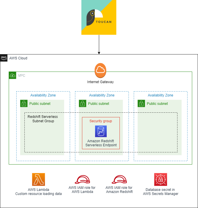
The following diagram depicts the architecture of our solution.

Architecture diagram

We use an AWS CloudFormation stack to deploy all the resources you need in your AWS account:

  • Networking components – This includes a VPC, three public subnets, an internet gateway, and a security group to host the Redshift Serverless endpoint. In this post, we use public subnets to facilitate data access from external sources such as Toucan instances. In this case, the data in Redshift Serverless is still protected by the security group that restricts incoming traffic, and by the database credentials. For a production workload, it is recommended to keep traffic in the Amazon network. For that, you can set the Redshift Serverless endpoints in private subnets, and deploy Toucan in your AWS account through the AWS Marketplace.
  • Redshift Serverless components – This includes a Redshift Serverless namespace and workgroup. The Redshift Serverless workspace is publicly accessible to facilitate the connection from Toucan instances. The database name and the administrator user name are defined as parameters when deploying the CloudFormation stack, and the administrator password is created in AWS Secrets Manager. In this post, we use database credentials to connect to Redshift Serverless, but Toucan also supports connection with AWS credentials and AWS Identity and Access Management (IAM) profiles.
  • Custom resources – The CloudFormation stack includes a custom resource, which is an AWS Lambda function that loads shark attacks data automatically in your Redshift Serverless database when the CloudFormation stack is created.
  • IAM roles and permissions – Finally, the CloudFormation stack includes all IAM roles associated with services previously mentioned to interact with other AWS resources in your account.

In the following sections, we provide all the instructions to connect Toucan with your data in Redshift Serverless, and guide you to build your data storytelling application.

Sample dataset

In this post, we use a custom dataset that lists all known shark attacks in the world, starting from 1900. You don’t have to import the data yourself; we use the Amazon Redshift COPY command to load the data when deploying the CloudFormation stack. The COPY command is one the fastest and most scalable methods to load data into Amazon Redshift. For more information, refer to Using a COPY command to load data.

The dataset contains 4,900 records with the following columns:

  • Date
  • Year
  • Decade
  • Century
  • Type
  • Zone_Type
  • Zone
  • Country
  • Activity
  • Sex
  • Age
  • Fatal
  • Time
  • Species
  • href (a PDF link with the description of the context)
  • Case_Number

Prerequisites

For this solution, you should have the following prerequisites:

  • An AWS account. If you don’t have one already, see the instructions in Sign Up for AWS.
  • An IAM user or role with permissions on AWS resources used in this solution.
  • A Toucan free trial to build the data storytelling application.

Set up the AWS resources

You can launch the CloudFormation stack in any Region where Redshift Serverless is available.

  1. Choose Launch Stack to start creating the required AWS resources for this post:

  1. Specify the database name in Redshift Serverless (default is dev).
  2. Specify the administrator user name (default is admin).

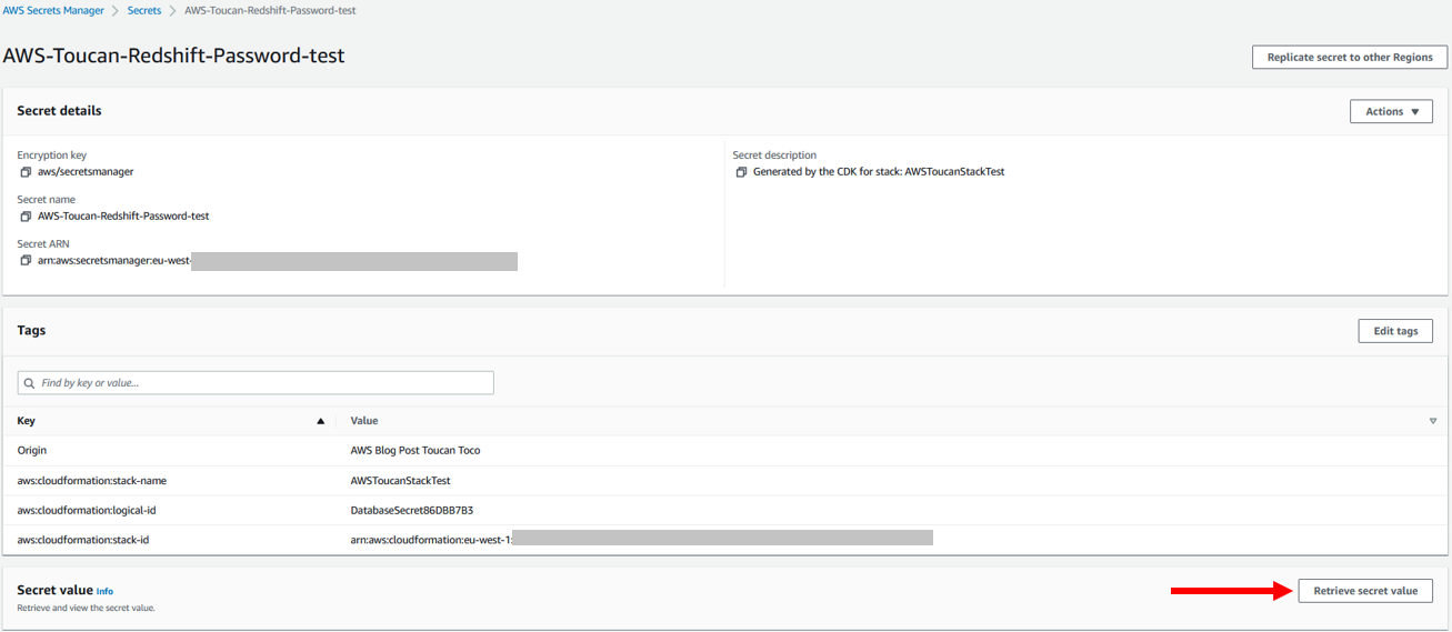
You don’t have to specify the database administrator password because it’s created in Secrets Manager by the CloudFormation stack. The secret’s name is AWS-Toucan-Redshift-Password. We use the secret value in subsequent steps.

Test the deployment

The CloudFormation stack takes a few minutes to deploy. When it’s complete, you can confirm the resources were created. To access your data, you need to get the Redshift Serverless database credentials.

  1. On the Outputs tab for the CloudFormation stack, note the name of the Secrets Manager secret.

BDB-2389temp

  1. On the Secrets Manager console, navigate to the Amazon Redshift database secret and choose Retrieve secret value to get the database administrator user name and password.

  1. To make sure your Redshift Serverless database is available and contains the shark attacks dataset, open the Redshift Serverless workgroup on the Amazon Redshift console and choose Query data to access the query editor.
  2. Also note the Redshift Serverless endpoint, which you need to connect with Toucan.

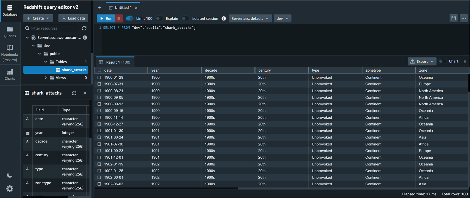
  1. In the Amazon Redshift query editor, run the following SQL query to view the shark attacks data:
SELECT * FROM "dev"."public"."shark_attacks";

Redshift Query Editor v2

Note that you need to change the name of the database in the SQL query if you change the default value when launching the CloudFormation stack.

You have configured Redshift Serverless in your AWS account and uploaded the shark attacks dataset. Now it’s time to use this data by building a storytelling application.

Launch your Toucan free trial

The first step is to access Toucan platform through the Toucan free trial.

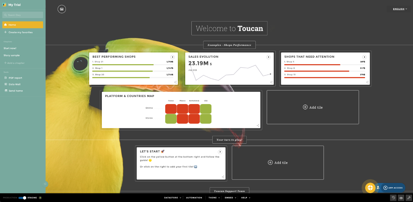
Fill the form and complete the signup steps. You then arrive in the Storytelling Studio, in Staging mode. Feel free to explore what has been already created.

Toucan Home page

Connect Redshift Serverless with Toucan

To connect Redshift Serverless and Toucan, complete the following steps:

  1. Choose Datastore at the bottom of the Toucan Storytelling Studio.
  2. Choose Connectors.

Toucan is natively integrated with Redshift Serverless with AnyConnect.

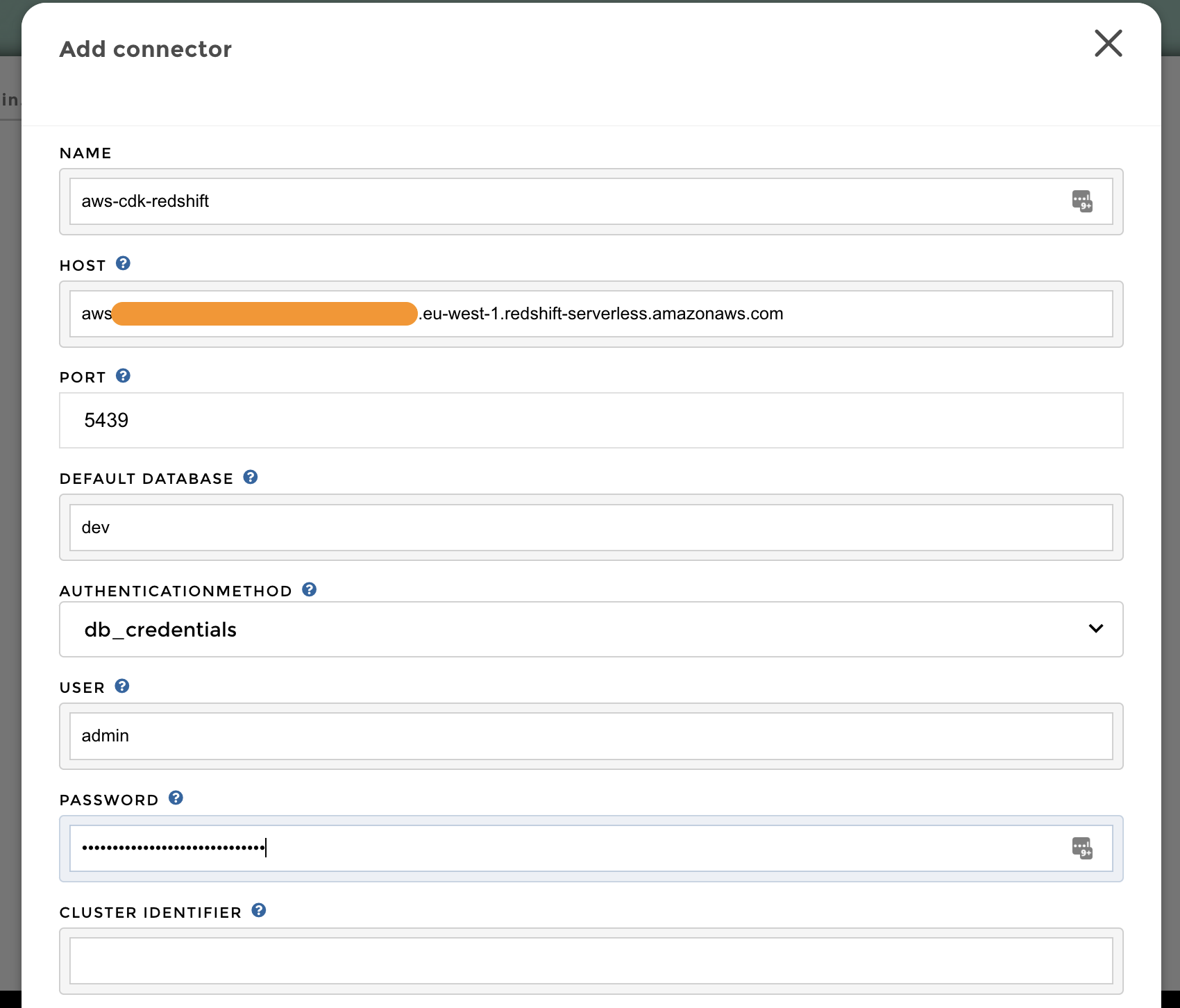
  1. Search for the Amazon Redshift connector, and complete the form with the following information:
    • Name – The name of the connector in Toucan.
    • Host – Your Redshift Serverless endpoint.
    • Port – The listening port of your Amazon Redshift database (5439).
    • Default Database – The name of the database to connect to (dev by default, unless edited in the CloudFormation stack parameters).
    • Authentication Method – The authentication mechanism to connect to Redshift Serverless. In this case, we use database credentials.
    • User – The user name to use for authentication with Redshift Serverless (admin by default, unless edited in the CloudFormation stack parameters).
    • Password – The password to use for authentication with Redshift Serverless (you should retrieve it from Secrets Manager; the secret’s name is AWS-Toucan-Redshift-Password).

Toucan connection

Create a live query

You are now connected to Redshift Serverless. Complete the following steps to create a query:

  1. On the home page, choose Add tile to create a new visualization.

Toucan new tile

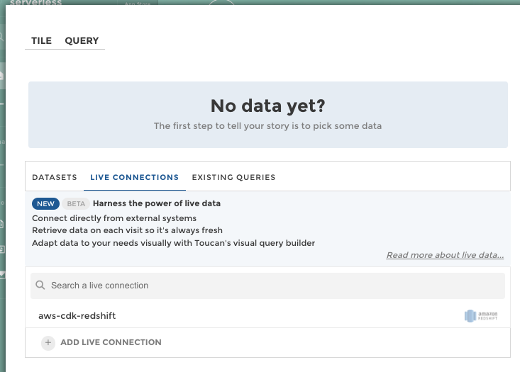
  1. Choose the Live Connections tab, then choose the Amazon Redshift connector you created in the previous step.

Toucan Live Connection

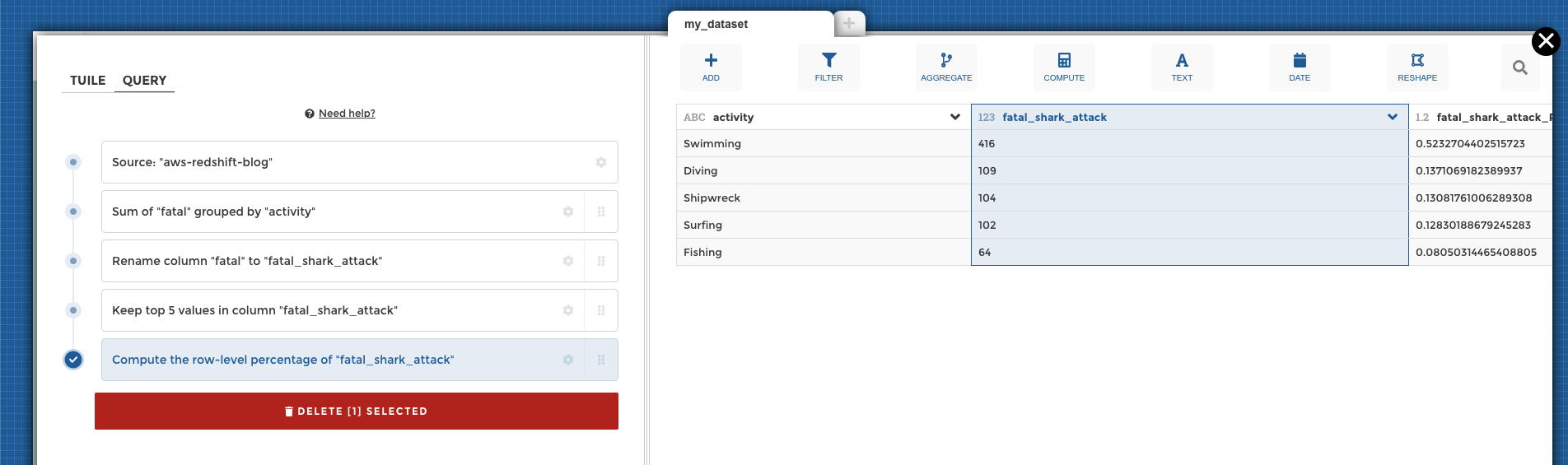
The Toucan trial guides you in building your first live query, in which you can transform your data without writing code using the Toucan YouPrep module.

For instance, as shown in the following screenshot, you can use this no-code interface to compute the sum of fatal shark attacks by activities, get the top five, and calculate the percentage of the total.

Toucan query data

Build your first chart

When your data is ready, choose the Tile tab and complete the form that helps you build charts.

For example, you can configure a leaderboard of the five most dangerous activities, and add a highlight for activities with more than 100 attacks.

Choose Save Changes to save your work and go back to the home page.

Toucan chart builder

Publish and share your work

Until this stage, you have been working in working in Staging mode. To make your work available to everyone, you need to publish it into Production.

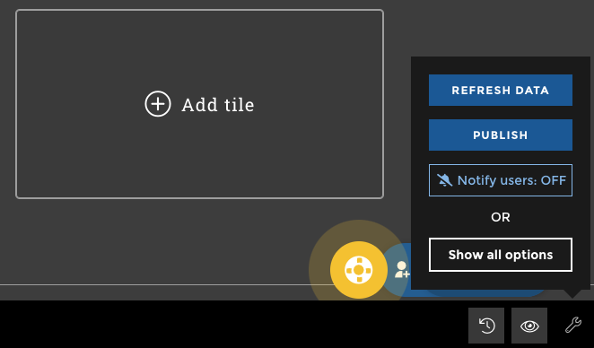
On the bottom right of the home page, choose the eye icon to preview your work by putting yourself in the shoes of your future end-users. You can then choose Publish to make your work available to all.

Toucan publish

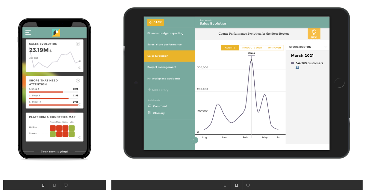
Toucan also offers multiple embedding options to make your charts easier for end-users to access, such as mobile and tablet.

Toucan multi devices

Following these steps, you connected to Redshift Serverless, transformed the data with the Toucan no-code interface, and built data visualizations for business end-users. The Toucan trial guides you in every stage of this process to help you get started.

Redshift Serverless and Toucan guided analytics provide an efficient approach to increase the adoption rate of BI tools by decreasing infrastructure work for data engineers, and by simplifying dashboard understanding for business end-users. This post only covered a small part of what Redshift Serverless and Toucan offer, so feel free to explore other functionalities in the Amazon Redshift Serverless documentation and Toucan documentation.

Clean up

Some of the resources deployed in this post through the CloudFormation template incur costs as long as they’re in use. Be sure to remove the resources and clean up your work when you’re finished in order to avoid unnecessary cost.

On the CloudFormation console, choose Delete stack to remove all resources.

Conclusion

This post showed you how to set up an end-to-end architecture for guided analytics with Redshift Serverless and Toucan.

This solution benefits from the scalability of Redshift Serverless, which enables you to store, transform, and expose data in a cost-efficient way, and without any infrastructure to manage. Redshift Serverless natively integrates with Toucan, a guided analytics tool designed to be used by everyone, on any device.

Guided analytics focuses on communicating stories through data reports. By setting intentional constraints on customization options, Toucan makes it easy for data owners to build meaningful dashboards with a clear and concise message for end-users. It works for both your internal and external customers, on an unlimited number of use cases.

Try it now with our CloudFormation template and a free Toucan trial!


About the Authors


Louis
Louis Hourcade
is a Data Scientist in the AWS Professional Services team. He works with AWS customer across various industries to accelerate their business outcomes with innovative technologies. In his spare time he enjoys running, climbing big rocks, and surfing (not so big) waves.


Benjamin
Benjamin Menuet
is a Data Architect with AWS Professional Services. He helps customers develop big data and analytics solutions to accelerate their business outcomes. Outside of work, Benjamin is a trail runner and has finished some mythic races like the UTMB.


Xavier
Xavier Naunay
is a Data Architect with AWS Professional Services. He is part of the AWS ProServe team, helping enterprise customers solve complex problems using AWS services. In his free time, he is either traveling or learning about technology and other cultures.


Django
Django Bouchez
is a Solution Engineer at Toucan. He works alongside the Sales team to provide support on technical and functional validation and proof, and is also helping R&D demo new features with Cloud Partners like AWS. Outside of work, Django is a homebrewer and practices scuba diving and sport climbing.

How to use AWS Private Certificate Authority short-lived certificate mode

Post Syndicated from Zachary Miller original https://aws.amazon.com/blogs/security/how-to-use-aws-private-certificate-authority-short-lived-certificate-mode/

AWS Private Certificate Authority (AWS Private CA) is a highly available, fully managed private certificate authority (CA) service that you can use to create CA hierarchies and issue private X.509 certificates. You can use these private certificates to establish endpoints for TLS encryption, cryptographically sign code, authenticate users, and more.

Based on customer feedback for prorated certificate pricing options, AWS Private CA now offers short-lived certificate mode, a lower cost mode of AWS Private CA that is designed to issue short-lived certificates. In this blog post, we will compare the original general-purpose and new short-lived CA modes and discuss use cases for each of them.

The general-purpose mode of AWS Private CA supports certificates of any validity period. The addition of short-lived CA mode is intended to facilitate use cases where you want certificates with a short validity period, defined as 7 days or less. Keep in mind this doesn’t mean that the root CA certificate must also be short lived. Although a typical root CA certificate is valid for 10 years, you can customize the certificate validity period for CAs in either mode when you install the CA certificate.

You select the CA mode when you create a certificate authority. The CA mode cannot be changed for an existing CA. Both modes (general-purpose and short-lived) have distinct pricing for the different use cases that they support.

The short-lived CA mode offers an accessible pricing model for customers who need to issue certificates with a short-term validity period. You can use these short-lived certificates for on-demand AWS workloads and align the validity of the certificate with the lifetime of the certificate holder. For example, if you’re using certificate-based authentication for a virtual workstation that is rebuilt each day, you can configure your certificates to expire after 24 hours.

In this blog post, we will compare the two CA modes, examine their pricing models, and discuss several potential use cases for short-lived certificates. We will also provide a walkthrough that shows you how to create a short-lived mode CA by using the AWS Command Line Interface (AWS CLI). To create a short-lived mode CA using the AWS Management Console, see Procedure for creating a CA (console).

Comparing general-purpose mode CAs to short-lived mode CAs

You might be wondering, “How is the short-lived CA mode different from the general-purpose CA mode? I can already create certificates with a short validity period by using AWS Private CA.” The key difference between these two CA modes is cost. Short-lived CA mode is priced to better serve use cases where you reissue private certificates frequently, such as for certificate-based authentication (CBA).

With CBA, users can authenticate once and then seamlessly access resources, including Amazon WorkSpaces and Amazon AppStream 2.0, without re-entering their credentials. This use case demonstrates the security value of short-lived certificates. A short validity period for the certificate reduces the impact of a compromised certificate because the certificate can only be used for authentication during a small window before it’s automatically invalidated. This method of authentication is useful for customers who are looking to adopt a Zero Trust security strategy.

Before the release of the short-lived CA mode, using AWS Private CA for CBA could be cost prohibitive for some customers. This is because CBA needs a new certificate for each user at regular intervals, which can require issuing a high volume of certificates. The best practice for CBA is to use short-lived CA mode, which can issue certificates at a lower cost that can be used to authenticate a user and then expire shortly afterward.

Let’s take a closer look at the pricing models for the two CA modes that are available when you use AWS Private CA.

Pricing model comparison

You can issue short-lived certificates from both the general-purpose and short-lived CA modes of AWS Private CA. However, the general-purpose mode CAs incur a monthly charge of $400 per CA. The cost of issuing certificates from a general-purpose mode CA is based on the number of certificates that you issue per month, per AWS Region.

The following table shows the pricing tiers for certificates issued by AWS Private CA by using a general-purpose mode CA.

Number of private certificates created each month (per Region) Price (per certificate)
1–1,000 $0.75 USD
1,001–10,000 $0.35 USD
10,001 and above $0.001 USD

The short-lived mode CA will only incur a monthly charge of $50 per CA. The cost of issuing certificates from a short-lived mode CA is the same regardless of the volume of certificates issued: $0.058 per certificate. This pricing structure is more cost effective than general-purpose mode if you need to frequently issue new, short-lived certificates for a use case like certificate-based authentication. Figure 1 compares costs between modes at different certificate volumes.

Figure 1: Cost comparison of AWS Private CA modes

Figure 1: Cost comparison of AWS Private CA modes

It’s important to note that if you already issue a high volume of certificates each month from AWS Private CA, the short-lived CA mode might not be more cost effective than the general-purpose mode. Consider a customer who has one CA and issues 80,000 certificates per month using the general-purpose CA mode: This will incur a total monthly cost of $4,370. A breakdown of the total cost per month in this scenario is as follows.

1 private CA x 400 USD per month = 400 USD per month for operation of AWS Private CA

Tiered price for 80,000 issued certificates:
1,000 issued certificates x 0.75 USD = 750 USD
9,000 issued certificates x 0.35 USD = 3,150 USD
70,000 issued certificates x 0.001 USD = 70 USD
Total tier cost: 750 USD + 3,150 USD + 70 USD = 3,970 USD per month for certificates issued
400 USD for instances + 3,970 USD for certificate issued = 4,370 USD
Total cost (monthly): 4,370 USD

Now imagine that same customer chose to use a short-lived mode CA to issue the same number of private certificates. Although the cost per month of the short-lived mode CA instance is lower, the price of issuing short-lived certificates would still be greater than the 70,000 certificates issued at a cost of $0.001 with the general-purpose mode CA. The total cost of issuing this many certificates from a single short-lived mode CA is $4,690. A breakdown of the total cost per month in this scenario is as follows.

1 private CA x 50 USD per month = 50 USD per month for operation of AWS Private CA (short-lived CA mode)

Price for 80,000 issued certificates (short-lived CA mode):
80,000 issued certificates x 0.058 USD = 4,640 USD
50 USD for instances + 4,640 USD for certificate issued = 4,690 USD
Total cost (monthly): 4,690 USD

At very high volumes of certificate issuance, the short-lived CA mode is not as cost effective as the general-purpose CA mode. It’s important to consider the volume of certificates that your organization will be issuing when you decide which CA mode to use. Figure 1 shows the cost difference at various volumes of certificate issuance. This difference will vary based on the number of certificates issued, as well as the number of CAs that your organization used.

You should also evaluate the various use cases that your organization has for using private certificates. For example, private certificates that are used to terminate TLS traffic typically have a validity of a year or more, meaning that the short-lived CA mode could not facilitate this use case. The short-lived CA mode can only issue certificates with a validity of 7 days or less.

However, you can create multiple private CAs and select the appropriate certificate authority mode for each CA based on your requirements. We recommend that you evaluate your use cases and estimate your certificate volume when you consider which CA mode to use.

In general, you should use the new short-lived CA mode for use cases where you require certificates with a short validity period (less than 7 days) and you are not planning to issue more than 75,000 certificates per month. You should use the general-purpose CA mode for scenarios where you need to issue certificates with a validity period of more than 7 days, or when you need short-lived certificates but will be issuing very high volumes of certificates each month (for example, over 75,000).

Use cases

The short-lived certificate feature was initially developed for certificate-based authentication with Amazon WorkSpaces and Amazon AppStream 2.0. For a step-by-step guide on how to configure certificate-based authentication for Amazon Workspaces, see How to configure certificate-based authentication for Amazon WorkSpaces. However, there are other ways to get value from the AWS Private CA short-lived CA mode, which we will describe in the following sections.

IAM Roles Anywhere

For customers who use AWS Identity and Access Management (IAM) Roles Anywhere, you might want to reduce the time period for which a certificate can be used to retrieve temporary credentials to assume an IAM role. If you frequently issue X.509 certificates to servers outside of AWS for use with IAM Roles Anywhere, and you want to use short-lived certificates, the pricing model for short-lived CA mode will be more cost effective in most cases (see Figure 1).

Short-lived credentials are useful for administrative personas that have broad permissions to AWS resources. For instance, you might use IAM Roles Anywhere to allow an entity outside AWS to assume an IAM role with the AdministratorAccess AWS managed policy attached. To help manage the risk of this access pattern, we want the certificate to expire relatively quickly, which reduces the time period during which a compromised certificate could potentially be used to authenticate to a highly privileged IAM role.

Furthermore, IAM Roles Anywhere requires that you manually upload a certificate revocation list (CRL), and does not support the CRL and Online Certificate Status Protocol (OCSP) mechanisms that are native to AWS Private CA. Using short-lived certificates is a way to reduce the impact of a potential credential compromise without needing to configure revocation for IAM Roles Anywhere. The need for certificate revocation is greatly reduced if the certificates are only valid for a single day and can’t be used to retrieve temporary credentials to assume an IAM role after the certificate expires.

Mutual TLS between workloads

Consider a highly sensitive workload running on Amazon Elastic Kubernetes Service (Amazon EKS). AWS Private CA supports an open-source plugin for cert-manager, a widely adopted solution for TLS certificate management in Kubernetes, that offers a more secure CA solution for Kubernetes containers. You can use cert-manager and AWS Private CA to issue certificates to identify cluster resources and encrypt data in transit with TLS.

If you use mutual TLS (mTLS) to protect network traffic between Kubernetes pods, you might want to align the validity period of the private certificates with the lifetime of the pods. For example, if you rebuild the worker nodes for your EKS cluster each day, you can issue certificates that expire after 24 hours and configure your application to request a new short-lived certificate before the current certificate expires.

This enables resource identification and mTLS between pods without requiring frequent revocation of certificates that were issued to resources that no longer exist. As stated previously, this method of issuing short-lived certificates is possible with the general-purpose CA mode—but using the new short-lived CA mode makes this use case more cost effective for customers who issue fewer than 75,000 certificates each month.

Create a short-lived mode CA by using the AWS CLI

In this section, we show you how to use the AWS CLI to create a new private certificate authority with the usage mode set to SHORT_LIVED_CERTIFICATE. If you don’t specify a usage mode, AWS Private CA creates a general-purpose mode CA by default. We won’t use a form of revocation, because the short-lived CA mode makes revocation less useful. The certificates expire quickly as part of normal operations. For more examples of how to create CAs with the AWS CLI, see Procedure for creating a CA (CLI). For instructions to create short-lived mode CAs with the AWS console, see Procedure for creating a CA (Console).

This walkthrough has the following prerequisites:

  1. A terminal with the .aws configuration directory set up with a valid default Region, endpoint, and credentials. For information about configuring your AWS CLI environment, see Configuration and credential file settings.
  2. An AWS Identity and Access Management (IAM) user or role that has permissions to create a certificate authority by using AWS Private CA.
  3. A certificate authority configuration file to supply when you create the CA. This file provides the subject details for the CA certificate, as well as the key and signing algorithm configuration.

    Note: We provide an example CA configuration file, but you will need to modify this example to meet your requirements.

To use the create-certificate-authority command with the AWS CLI

  1. We will use the following ca_config.txt file to create the certificate authority. You will need to modify this example to meet your requirements.
    {
       "KeyAlgorithm":"RSA_2048",
       "SigningAlgorithm":"SHA256WITHRSA",
       "Subject":{
          "Country":"US",
          "Organization":"Example Corp",
          "OrganizationalUnit":"Sales",
          "State":"WA",
          "Locality":"Seattle",
          "CommonName":"Example Root CA G1"
       }
    }

  2. Enter the following command to create a short-lived mode root CA by using the parameters supplied in the ca_config.txt file.

    Note: Make sure that ca_config.txt is located in your current directory, or specify the full path to the file.

    aws acm-pca create-certificate-authority \
    --certificate-authority-configuration file://ca_config.txt \
    --certificate-authority-type "ROOT" \
    --usage-mode SHORT_LIVED_CERTIFICATE \
    --tags Key=usageMode,Value=SHORT_LIVED_CERTIFICATE

  3. Use the describe-certificate-authority command to view the status of your new root CA. The status will show Pending_Certificate, until you install a self-signed root CA certificate. You will need to replace the certificate authority Amazon Resource Name (ARN) in the following command with your own CA ARN.

    sh-4.2$ aws acm-pca describe-certificate-authority --certificate-authority-arn arn:aws:acm-pca:region:account:certificate-authority/CA_ID

    The output of this command is as follows:

    {
        "CertificateAuthority": {
            "Arn": "arn:aws:acm-pca:region:account:certificate-authority/CA_ID",
            "OwnerAccount": "account",
            "CreatedAt": "2022-11-02T23:12:46.916000+00:00",
            "LastStateChangeAt": "2022-11-02T23:12:47.779000+00:00",
            "Type": "ROOT",
            "Status": "PENDING_CERTIFICATE",
            "CertificateAuthorityConfiguration": {
                "KeyAlgorithm": "RSA_2048",
                "SigningAlgorithm": "SHA256WITHRSA",
                "Subject": {
                    "Country": "US",
                    "Organization": "Example Corp",
                    "OrganizationalUnit": "Sales",
                    "State": "WA",
                    "CommonName": "Example Root CA G1",
                    "Locality": "Seattle"
                }
            },
            "RevocationConfiguration": {
                "CrlConfiguration": {
                    "Enabled": false
                },
                "OcspConfiguration": {
                    "Enabled": false
                }
            },
            "KeyStorageSecurityStandard": "FIPS_140_2_LEVEL_3_OR_HIGHER",
            "UsageMode": "SHORT_LIVED_CERTIFICATE"
        }
    }

  4. Generate a certificate signing request for your root CA certificate by running the following command. Make sure to replace the certificate authority ARN in the command with your own CA ARN.

    aws acm-pca get-certificate-authority-csr \
    --certificate-authority-arn arn:aws:acm-pca:region:account:certificate-authority/CA_ID \
    --output text > ca.csr

  5. Using the ca.csr file from the previous step as the argument for the --csr parameter, issue the root certificate with the following command. Make sure to replace the certificate authority ARN in the command with your own CA ARN.

    aws acm-pca issue-certificate \
    --certificate-authority-arn arn:aws:acm-pca:region:account:certificate-authority/CA_ID \
    --csr fileb://ca.csr \
    --signing-algorithm SHA256WITHRSA \
    --template-arn arn:aws:acm-pca:::template/RootCACertificate/V1 \
    --validity Value=10,Type=YEARS

  6. The response will include the CertificateArn for the issued root CA certificate. Next, use your CA ARN and the certificate ARN provided in the response to retrieve the certificate by using the get-certificate CLI command, as follows.

    aws acm-pca get-certificate \
    --certificate-authority-arn arn:aws:acm-pca:region:account:certificate-authority/CA_ID \
    --certificate-arn arn:aws:acm-pca:region:account:certificate-authority/CA_ID/certificate/CERTIFICATE_ID \
    --output text > cert.pem

  7. Notice that we created a new file, cert.pem, that contains the certificate we retrieved in the previous command. We will import this certificate to our short-lived mode root CA by running the following command. Make sure to replace the certificate authority ARN in the command with your own CA ARN.

    aws acm-pca import-certificate-authority-certificate \
    --certificate-authority-arn arn:aws:acm-pca:region:account:certificate-authority/CA_ID \
    --certificate fileb://cert.pem

  8. Check the status of your short-lived mode CA again by using the describe-certificate-authority command. Make sure to replace the certificate authority ARN in the following command with your own CA ARN.

    sh-4.2$ aws acm-pca describe-certificate-authority \
    > --certificate-authority-arn arn:aws:acm-pca:region:account:certificate-authority/CA_ID \
    > --output json

    The output of this command is as follows:

    {
        "CertificateAuthority": {
            "Arn": "arn:aws:acm-pca:region:account:certificate-authority/CA_ID",
            "OwnerAccount": "account",
            "CreatedAt": "2022-11-02T23:12:46.916000+00:00",
            "LastStateChangeAt": "2022-11-02T23:39:23.482000+00:00",
            "Type": "ROOT",
            "Serial": "serial",
            "Status": "ACTIVE",
            "NotBefore": "2022-11-02T22:34:50+00:00",
            "NotAfter": "2032-11-02T23:34:50+00:00",
            "CertificateAuthorityConfiguration": {
                "KeyAlgorithm": "RSA_2048",
                "SigningAlgorithm": "SHA256WITHRSA",
                "Subject": {
                    "Country": "US",
                    "Organization": "Example Corp",
                    "OrganizationalUnit": "Sales",
                    "State": "WA",
                    "CommonName": "Example Root CA G1",
                    "Locality": "Seattle"
                }
            },
            "RevocationConfiguration": {
                "CrlConfiguration": {
                    "Enabled": false
                },
                "OcspConfiguration": {
                    "Enabled": false
                }
            },
            "KeyStorageSecurityStandard": "FIPS_140_2_LEVEL_3_OR_HIGHER",
            "UsageMode": "SHORT_LIVED_CERTIFICATE"
        }
    }

  9. Great! As shown in the output from the preceding command, the new short-lived mode root CA has a status of ACTIVE, meaning it can now issue certificates. This certificate authority will be able to issue end-entity certificates that have a validity period of up to 7 days, as shown in the UsageMode: SHORT_LIVED_CERTIFICATE parameter.

Conclusion

In this post, we introduced the short-lived CA mode that is offered by AWS Private CA, explained how it differs from the general-purpose CA mode, and compared the pricing models for both CA modes. We also provided some recommendations for choosing the appropriate CA mode based on your certificate issuance volume and use cases. Finally, we showed you how to create a short-lived mode CA by using the AWS CLI.

Get started using AWS Private CA, and consult the AWS Private CA User Guide for more details on the short-lived CA mode.

If you have feedback about this post, submit comments in the Comments section below. If you have questions about this post, start a new thread on the AWS Certificate Manager re:Post or contact AWS Support.

Want more AWS Security news? Follow us on Twitter.

Zach Miller

Zach Miller

Zach is a Senior Security Specialist Solutions Architect at AWS. His background is in data protection and security architecture, focused on a variety of security domains, including cryptography, secrets management, and data classification. Today, he is focused on helping enterprise AWS customers adopt and operationalize AWS security services to increase security effectiveness and reduce risk.

Rushir Patel

Rushir Patel

Rushir is a Senior Security Specialist at AWS focused on data protection and cryptography services. His goal is to make complex topics simple for customers and help them adopt better security practices. Prior to AWS, he worked in security product management, engineering, and operations roles.

Trevor Freeman

Trevor Freeman

Trevor is an innovative and solutions-oriented Product Manager at Amazon Web Services, focusing on AWS Private CA. With over 20 years of experience in software and service development, he became an expert in Cloud Services, Security, Enterprise Software, and Databases. Being adept in product architecture and quality assurance, Trevor takes great pride in providing exceptional customer service.

Improve security of Amazon RDS master database credentials using AWS Secrets Manager

Post Syndicated from Vinod Santhanam original https://aws.amazon.com/blogs/security/improve-security-of-amazon-rds-master-database-credentials-using-secrets-manager/

Amazon Relational Database Service (Amazon RDS) makes it simpler to set up, operate, and scale a relational database in the AWS Cloud. AWS Secrets Manager helps you manage, retrieve, and rotate database credentials, API keys, and other secrets.

Amazon RDS now offers integration with Secrets Manager to manage master database credentials. You no longer have to manage master database credentials, such as creating a secret in Secrets Manager or setting up rotation, because Amazon RDS does it for you.

In this blog post, you will learn how to set up an Amazon RDS database instance and use the Secrets Manager integration to manage master database credentials. You will also learn how to set up alternating users rotation for application credentials.

Benefits of the integration

Managing Amazon RDS master database credentials with Secrets Manager provides the following benefits:

  • Amazon RDS automatically generates and helps secure master database credentials, so that you don’t have to do the heavy lifting of securely managing credentials.
  • Amazon RDS automatically stores and manages database credentials in Secrets Manager.
  • Amazon RDS rotates database credentials regularly without requiring application changes.
  • Secrets Manager helps to secure database credentials from human access and plaintext view.
  • Secrets Manager allows retrieval of database credentials using its API or the console.
  • Secrets Manager allows fine-grained control of access to database credentials in secrets using AWS Identity and Access Management (IAM).
  • You can separate database encryption from credentials encryption with different AWS Key Management Service (AWS KMS) keys.
  • You can monitor access to database credentials with AWS CloudTrail and Amazon CloudWatch.

Walkthrough

In this blog post, we’ll show you how to use the console to do the following:

  • Manage master database credentials for new Amazon RDS instances in Secrets Manager. We will use the MySQL engine, but you can also use this process for other Amazon RDS database engines.
  • Use the managed master database secret to set up alternating users rotation for a new database user.

Manage Amazon RDS master database credentials in Secrets Manager

In this section, you will create a database instance with Secrets Manager integration.

To manage Amazon RDS master database credentials in Secrets Manager:

  1. Open the Amazon RDS console and choose Create database.
  2. For Choose a database creation method, choose Standard create.
  3. In Engine options, for Engine type, choose MySQL.
  4. In Settings, under Credentials Settings, select Manage master credentials in AWS Secrets Manager.
    Figure 1: Select Secrets Manager integration

    Figure 1: Select Secrets Manager integration

  5. You will have the option to encrypt the managed master database credentials. In this example, we will use the default KMS key.
    Figure 2: Choose KMS key

    Figure 2: Choose KMS key

  6. (Optional) Choose other settings to meet your requirements. For more information, see Settings for DB instances.
  7. Choose Create Database, and wait a few minutes for the database to be created.
  8. After the database is created, from the Instances dashboard in the Amazon RDS console, navigate to your new Amazon RDS instance.
  9. Choose the Configuration tab, and under Master Credentials ARN, you will find the secret that contains your master database credentials.

Create a new database user by using the master database credentials

In this section you will learn how to create and secure a credential that could be used in your application to connect to the database. You will learn how to access the master database credentials and use the master database credentials to create and set up rotation on child (application) credentials.

To create a new database user by using the master database credentials

  1. Retrieve the master database credentials from Secrets Manager as follows:
    1. Choose the Configuration tab of your RDS instance dashboard, and under Master Credentials ARN, choose Manage in Secrets Manager to open your managed master database secret in Secrets Manager.
      Figure 3: View DB configuration

      Figure 3: View DB configuration

    2. You can see that Amazon RDS has added some system tags to the secret and that rotation is turned on by default.
      Figure 4: View secret details

      Figure 4: View secret details

    3. To see the password, in the Secret value section, choose Retrieve secret value.

    Note: Your applications can retrieve these credentials by using the AWS Command Line Interface (AWS CLI) or AWS SDK if they have IAM permission to read the secret.

  2. In MySQL Workbench, log in to your Amazon RDS database as the master database by using the credentials that you just retrieved from the secret. For more information, see Connecting to a DB instance running the MySQL database engine.
  3. For the master database, create a new database user with the permissions that you want by running the following SQL command. Make sure to replace <password> with your own information, and make sure to use a strong password.

    CREATE USER 'child'@'%' IDENTIFIED by <password>;

For more information about creating users, see the MySQL documentation.

Set up alternating users rotation for the new database user

In this section, you will learn how to use the master database credential to set up multi-user rotation for application credentials.

To set up alternating users rotation

  1. In the Secrets Manager console, under Secrets, choose Store a new secret.
  2. For Secret type, select Credentials for Amazon RDS database.
  3. In the Credentials section, enter the username and password of the new database user.
  4. In the Database section, select your Amazon RDS instance, and then choose Next, as shown in Figure 5.
    Figure 5: Select the RDS instance

    Figure 5: Select the RDS instance

  5. On the Configure secret page, give the secret a name and description. No other configuration is needed.
  6. On the Configure rotation – optional page, turn on Automatic rotation.
    Figure 6: Select automatic rotation

    Figure 6: Select automatic rotation

  7. In the Rotation schedule section, configure the rotation schedule according to your needs.
  8. In the Rotation function section, do the following:
    1. Enter a descriptive name for the Lambda function that will be created.
    2. For Use separate credentials to rotate this secret, select Yes.
    3. For Secrets, choose the master database secret that was created by Amazon RDS.

      Note: To find the name of your master database secret, in the Amazon RDS console, on your Amazon RDS instance details page, choose the Configuration tab and then see the Master Credentials ARN.

    Figure 7: Select separate credentials for rotation

    Figure 7: Select separate credentials for rotation

  9. Choose Next, and then on the Review page, choose Store.

It will take a few minutes for the Secrets Manager workflow to set up the rotation Lambda function before the new database user secret is ready to be rotated.

To check that rotation is enabled

  1. In the Secrets Manager console, navigate to the new database user secret.
    Figure 8: View the child secret

    Figure 8: View the child secret

  2. In the Rotation configuration section, verify that Rotation status is Enabled.
    Figure 9: Verify the rotation status

    Figure 9: Verify the rotation status

For more details and troubleshooting on this process, see Set up alternating users rotation for AWS Secrets Manager.

Clean up the resources

By deleting the Amazon RDS instance, you will automatically clean up the managed master database credential secret.

To delete the Amazon RDS instance

  1. Open the Amazon RDS console.
  2. From the navigation pane, choose Databases and then select the DB cluster to be modified.
  3. Choose Actions, and then choose Modify Cluster.
  4. Choose Disable deletion protection, and then choose Continue.
  5. Choose Apply immediately.
  6. From the Actions dropdown, choose Delete.
  7. (Optional) Use the menu to create final snapshots or automated backups of your Amazon RDS instance.
    Figure 10: Create snapshots and backups

    Figure 10: Create snapshots and backups

  8. When you’re ready, enter delete me.

For more information, see Deleting a DB instance.

To clean up alternating users rotation on the new database user secret

  1. In the Secrets Manager console, open the new database user secret.
    Figure 11: Select child secret

    Figure 11: Select child secret

  2. In the Rotation configuration section, choose the Lambda rotation function.
    Figure 12: View the rotation function

    Figure 12: View the rotation function

  3. In the Lambda console, under Application, select the application.
    Figure 13: Open application

    Figure 13: Open application

  4. On the Deployments tab, choose CloudFormation stack.
  5. Choose Delete and then follow the Delete menu steps. You might need to navigate to the root stack and choose Delete again. You might also need to disable termination protection for the stack. The console will guide you through that.
    Figure 14: Choose delete

    Figure 14: Choose delete

  6. Now that you have cleaned up rotation for the new database user secret, you need to delete the child secret. Navigate to the Secrets Manager console and select the secret that you want to delete.
  7. In the Actions dropdown, select Delete secret to delete the secret.
    Figure 15: Delete child secret

    Figure 15: Delete child secret

Summary

Amazon RDS integration with Secrets Manager helps you better secure and manage master DB credentials. This integration helps you store the credentials when the DB instances are created and eliminates the effort for you to set up credential rotation.

In this blog post, you learned how to do the following:

  1. Set up an Amazon RDS instance that uses Secrets Manager to store the master database credentials
  2. View the credentials in Secrets Manager and confirm that rotation is set up
  3. Use the master database credentials to create database user credentials
  4. Set up alternating users rotation on database user credentials

Additional resources

For instructions on how to create database users for other Amazon RDS engine types, see the following resources:

 
If you have feedback about this post, submit comments in the Comments section below. If you have questions about this post, contact AWS Support.

Want more AWS Security news? Follow us on Twitter.

Vinod Santhanam

Vinod Santhanam

Vinod is a Senior Technical Program Manager at AWS. He has over 17 years of experience in designing and developing software. He currently works with other AWS platform teams to build secure features for customers. Outside of work, he enjoys biking and exploring the beautiful trails and mountains in Pacific Northwest.

Adithya Solai

Adithya Solai

Adithya is a Software Development Engineer working on core backend features for AWS Secrets Manager. He graduated from the University of Maryland — College Park with a B.S. in Computer Science. He is passionate about social work in education. He enjoys reading, chess, and hip-hop/r&b music.

­­Use fuzzy string matching to approximate duplicate records in Amazon Redshift

Post Syndicated from Sean Beath original https://aws.amazon.com/blogs/big-data/use-fuzzy-string-matching-to-approximate-duplicate-records-in-amazon-redshift/

Amazon Redshift is a fully managed, petabyte-scale data warehouse service in the cloud. Amazon Redshift enables you to run complex SQL analytics at scale and performance on terabytes to petabytes of structured and unstructured data, and make the insights widely available through popular business intelligence (BI) and analytics tools.

It’s common to ingest multiple data sources into Amazon Redshift to perform analytics. Often, each data source will have its own processes of creating and maintaining data, which can lead to data quality challenges within and across sources.

One challenge you may face when performing analytics is the presence of imperfect duplicate records within the source data. Answering questions as simple as “How many unique customers do we have?” can be very challenging when the data you have available is like the following table.

Name Address Date of Birth
Cody Johnson 8 Jeffery Brace, St. Lisatown 1/3/1956
Cody Jonson 8 Jeffery Brace, St. Lisatown 1/3/1956

Although humans can identify that Cody Johnson and Cody Jonson are most likely the same person, it can be difficult to distinguish this using analytics tools. This identification of duplicate records also becomes nearly impossible when working on large datasets across multiple sources.

This post presents one possible approach to addressing this challenge in an Amazon Redshift data warehouse. We import an open-source fuzzy matching Python library to Amazon Redshift, create a simple fuzzy matching user-defined function (UDF), and then create a procedure that weights multiple columns in a table to find matches based on user input. This approach allows you to use the created procedure to approximately identify your unique customers, improving the accuracy of your analytics.

This approach doesn’t solve for data quality issues in source systems, and doesn’t remove the need to have a wholistic data quality strategy. For addressing data quality challenges in Amazon Simple Storage Service (Amazon S3) data lakes and data pipelines, AWS has announced AWS Glue Data Quality (preview). You can also use AWS Glue DataBrew, a visual data preparation tool that makes it easy for data analysts and data scientists to clean and normalize data to prepare it for analytics.

Prerequisites

To complete the steps in this post, you need the following:

The following AWS CloudFormation stack will deploy a new Redshift Serverless endpoint and an S3 bucket for use in this post.

BDB-2063-launch-cloudformation-stack

All SQL commands shown in this post are available in the following notebook, which can be imported into the Amazon Redshift Query Editor V2.

Overview of the dataset being used

The dataset we use is mimicking a source that holds customer information. This source has a manual process of inserting and updating customer data, and this has led to multiple instances of non-unique customers being represented with duplicate records.

The following examples show some of the data quality issues in the dataset being used.

In this first example, all three customers are the same person but have slight differences in the spelling of their names.

id name age address_line1 city postcode state
1 Cody Johnson 80 8 Jeffrey Brace St. Lisatown 2636 South Australia
101 Cody Jonson 80 8 Jeffrey Brace St. Lisatown 2636 South Australia
121 Kody Johnson 80 8 Jeffrey Brace St. Lisatown 2636 South Australia

In this next example, the two customers are the same person with slightly different addresses.

id name age address_line1 city postcode state
7 Angela Watson 59 3/752 Bernard Follow Janiceberg 2995 Australian Capital Territory
107 Angela Watson 59 752 Bernard Follow Janiceberg 2995 Australian Capital Territory

In this example, the two customers are different people with the same address. This simulates multiple different customers living at the same address who should still be recognized as different people.

id name age address_line1 city postcode state
6 Michael Hunt 69 8 Santana Rest St. Jessicamouth 2964 Queensland
106 Sarah Hunt 69 8 Santana Rest St. Jessicamouth 2964 Queensland

Load the dataset

First, create a new table in your Redshift Serverless endpoint and copy the test data into it by doing the following:

  1. Open the Query Editor V2 and log in using the admin user name and details defined when the endpoint was created.
  2. Run the following CREATE TABLE statement:
    create table customer (
        id smallint, 
        urid smallint,
        name varchar(100),
        age smallint,
        address_line1 varchar(200),
        city varchar(100),
        postcode smallint,
        state varchar(100)
    )
    ;

    Screenshot of CREATE TABLE statement for customer table being run successfully in Query Editor V2

  3. Run the following COPY command to copy data into the newly created table:
    copy customer (id, name, age, address_line1, city, postcode, state)
    from ' s3://redshift-blogs/fuzzy-string-matching/customer_data.csv'
    IAM_ROLE default
    FORMAT csv
    REGION 'us-east-1'
    IGNOREHEADER 1
    ;

  4. Confirm the COPY succeeded and there are 110 records in the table by running the following query:
    select count(*) from customer;

    Screenshot showing the count of records in the customer table is 110. Query is run in Query Editor V2

Fuzzy matching

Fuzzy string matching, more formally known as approximate string matching, is the technique of finding strings that match a pattern approximately rather than exactly. Commonly (and in this solution), the Levenshtein distance is used to measure the distance between two strings, and therefore their similarity. The smaller the Levenshtein distance between two strings, the more similar they are.

In this solution, we exploit this property of the Levenshtein distance to estimate if two customers are the same person based on multiple attributes of the customer, and it can be expanded to suit many different use cases.

This solution uses TheFuzz, an open-source Python library that implements the Levenshtein distance in a few different ways. We use the partial_ratio function to compare two strings and provide a result between 1–100. If one of the strings matches perfectly with a portion of the other, the partial_ratio function will return 100.

Weighted fuzzy matching

By adding a scaling factor to each of our column fuzzy matches, we can create a weighted fuzzy match for a record. This is especially useful in two scenarios:

  • We have more confidence in some columns of our data than others, and therefore want to prioritize their similarity results.
  • One column is much longer than the others. A single character difference in a long string will have much less impact on the Levenshtein distance than a single character difference in a short string. Therefore, we want to prioritize long string matches over short string matches.

The solution in this post applies weighted fuzzy matching based on user input defined in another table.

Create a table for weight information

This reference table holds two columns; the table name and the column mapping with weights. The column mapping is held in a SUPER datatype, which allows JSON semistructured data to be inserted and queried directly in Amazon Redshift. For examples on how to query semistructured data in Amazon Redshift, refer to Querying semistructured data.

In this example, we apply the largest weight to the column address_line1 (0.5) and the smallest weight to the city and postcode columns (0.1).

Using the Query Editor V2, create a new table in your Redshift Serverless endpoint and insert a record by doing the following:

  1. Run the following CREATE TABLE statement:
    CREATE TABLE ref_unique_record_weight_map(table_name varchar(100), column_mapping SUPER);

  2. Run the following INSERT statement:
    INSERT INTO ref_unique_record_weight_map VALUES (
        'customer',
        JSON_PARSE('{
        "colmap":[
        {
            "colname": "name",
            "colweight": 0.3
        },
        {
            "colname": "address_line1",
            "colweight": 0.5
        },
        {
            "colname": "city",
            "colweight": 0.1
        },
        {
            "colname": "postcode",
            "colweight": 0.1
        }
        ]
    }')
    );

  3. Confirm the mapping data has inserted into the table correctly by running the following query:
    select * from ref_unique_record_weight_map;

    Screenshot showing the result of querying the ref_unique_record_weight_map table in Query Editor V2

  4. To check all weights for the customer table add up to 1 (100%), run the following query:
    select  cm.table_name, 
            sum(colmap.colweight) as total_column_weight 
    from    ref_unique_record_weight_map cm, cm.column_mapping.colmap colmap 
    where   cm.table_name = 'customer'
    group by cm.table_name;

    Screenshot showing the total weight applied to the customer table is 1.0

User-defined functions

With Amazon Redshift, you can create custom scalar user-defined functions (UDFs) using a Python program. A Python UDF incorporates a Python program that runs when the function is called and returns a single value. In addition to using the standard Python functionality, you can import your own custom Python modules, such as the module described earlier (TheFuzz).

In this solution, we create a Python UDF to take two input values and compare their similarity.

Import external Python libraries to Amazon Redshift

Run the following code snippet to import the TheFuzz module into Amazon Redshift as a new library. This makes the library available within Python UDFs in the Redshift Serverless endpoint. Make sure to provide the name of the S3 bucket you created earlier.

CREATE OR REPLACE LIBRARY thefuzz LANGUAGE plpythonu 
FROM 's3://<your-bucket>/thefuzz.zip' 
IAM_ROLE default;

Create a Python user-defined function

Run the following code snippet to create a new Python UDF called unique_record. This UDF will do the following:

  1. Take two input values that can be of any data type as long as they are the same data type (such as two integers or two varchars).
  2. Import the newly created thefuzz Python library.
  3. Return an integer value comparing the partial ratio between the two input values.
CREATE OR REPLACE FUNCTION unique_record(value_a ANYELEMENT, value_b ANYELEMENT) 
RETURNS INTEGER IMMUTABLE
AS
$$
    from thefuzz import fuzz

    return fuzz.partial_ratio(value_a, value_b)
$$ LANGUAGE plpythonu;

You can test the function by running the following code snippet:

select unique_record('Cody Johnson'::varchar, 'Cody Jonson'::varchar)

The result shows that these two strings are have a similarity value of 91%.

Screenshot showing that using the created function on the Cody Johnson/Cody Jonson name example provides a response of 91

Now that the Python UDF has been created, you can test the response of different input values.

Alternatively, you can follow the amazon-redshift-udfs GitHub repo to install the f_fuzzy_string_match Python UDF.

Stored procedures

Stored procedures are commonly used to encapsulate logic for data transformation, data validation, and business-specific logic. By combining multiple SQL steps into a stored procedure, you can reduce round trips between your applications and the database.

In this solution, we create a stored procedure that applies weighting to multiple columns. Because this logic is common and repeatable regardless of the source table or data, it allows us to create the stored procedure once and use it for multiple purposes.

Create a stored procedure

Run the following code snippet to create a new Amazon Redshift stored procedure called find_unique_id. This procedure will do the following:

  1. Take one input value. This value is the table you would like to create a golden record for (in our case, the customer table).
  2. Declare a set of variables to be used throughout the procedure.
  3. Check to see if weight data is in the staging table created in previous steps.
  4. Build a query string for comparing each column and applying weights using the weight data inserted in previous steps.
  5. For each record in the input table that doesn’t have a unique record ID (URID) yet, it will do the following:
    1. Create a temporary table to stage results. This temporary table will have all potential URIDs from the input table.
    2. Allocate a similarity value to each URID. This value specifies how similar this URID is to the record in question, weighted with the inputs defined.
    3. Choose the closest matched URID, but only if there is a >90% match.
    4. If there is no URID match, create a new URID.
    5. Update the source table with the new URID and move to the next record.

This procedure will only ever look for new URIDs for records that don’t already have one allocated. Therefore, rerunning the URID procedure multiple times will have no impact on the results.

CREATE OR REPLACE PROCEDURE find_unique_id(table_name varchar(100)) AS $$
DECLARE
    unique_record RECORD;
    column_info RECORD;

    column_fuzzy_comparison_string varchar(MAX) := '0.0';
    max_simularity_value decimal(5,2) := 0.0;

    table_check varchar(100);
    temp_column_name varchar(100);
    temp_column_weight decimal(5,2);
    unique_record_id smallint := 0;
BEGIN
    /* 
        Check the ref_unique_record_weight_map table to see if there is a mapping record for the provided table.
        If there is no table, raise an exception
    */
    SELECT INTO table_check cm.table_name from ref_unique_record_weight_map cm where cm.table_name = quote_ident(table_name);
    IF NOT FOUND THEN
        RAISE EXCEPTION 'Input table ''%'' not found in mapping object', table_name;
        RETURN;
    END IF;

    /*
        Build query to be used to compare each column using the mapping record in the ref_unique_record_weight_map table.
        For each column specified in the mapping object, append a weighted comparison of the column
    */
    FOR column_info IN (
        select  colmap.colname::varchar(100) column_name, 
                colmap.colweight column_weight 
        from    ref_unique_record_weight_map cm, cm.column_mapping.colmap colmap 
        where   cm.table_name = quote_ident(table_name)
    ) LOOP
        temp_column_name = column_info.column_name;
        temp_column_weight = column_info.column_weight;
        
        column_fuzzy_comparison_string = column_fuzzy_comparison_string || 
            ' + unique_record(t1.' || 
            temp_column_name || 
            '::varchar, t2.' || 
            temp_column_name || 
            '::varchar)*' || 
            temp_column_weight;
    END LOOP;

    /* Drop temporary table if it exists */
    EXECUTE 'DROP TABLE IF EXISTS #unique_record_table';

    /*
        For each record in the source table that does not have a Unique Record ID (URID):
            1. Create a new temporary table holding all possible URIDs for this record (i.e. all URIDs that have are present). 
                Note: This temporary table will only be present while the simularity check is being calculated
            2. Update each possible URID in the temporary table with it's simularity to the record being checked
            3. Find the most simular record with a URID
                3a. If the most simular record is at least 90% simular, take it's URID (i.e. this is not a unique record, and matches another in the table)
                3b. If there is no record that is 90% simular, create a new URID (i.e. this is a unique record)
            4. Drop the temporary table in preparation for the next record
    */
    FOR unique_record in EXECUTE 'select * from ' || table_name || ' where urid is null order by id asc' LOOP

        RAISE INFO 'test 1';

        /* Create temporary table */
        EXECUTE '
            CREATE TABLE #unique_record_table AS 
            SELECT id, urid, 0.0::decimal(5,2) as simularity_value 
            FROM ' || table_name || '
            where urid is not null
            ';

        /* Update simularity values in temporary table */
        EXECUTE '
            UPDATE #unique_record_table  
            SET simularity_value = round(calc_simularity_value,2)::decimal(5,2)
            FROM (
                SELECT ' || column_fuzzy_comparison_string || ' as calc_simularity_value,
                        t2.id as upd_id
                FROM ' || table_name || ' t1
                INNER JOIN ' || table_name || ' t2
                ON t1.id <> t2.id
                AND t1.id = ' || quote_literal(unique_record.id) || '
                ) t
            WHERE t.upd_id = id
            ';

        /* Find largest simularity value */
        SELECT INTO max_simularity_value simularity_value FROM (
            SELECT  MAX(simularity_value) as simularity_value 
            FROM    #unique_record_table
        );

        /* If there is a >90% similar match, choose it's URID. Otherwise, create a new URID */
        IF max_simularity_value > 90 THEN
            SELECT INTO unique_record_id urid FROM (
                SELECT urid
                FROM #unique_record_table
                WHERE simularity_value = max_simularity_value
            );
        ELSE 
            EXECUTE 'select COALESCE(MAX(urid)+1,1) FROM ' || table_name INTO unique_record_id;
        END IF;
        
        /* Update table with new URID value */
        EXECUTE 'UPDATE ' || table_name || ' SET urid = ' || quote_literal(unique_record_id) || ' WHERE id = ' || quote_literal(unique_record.id);

        /* Drop temporary table and repeat process */
        EXECUTE 'DROP TABLE #unique_record_table';

        max_simularity_value = 0.0;
    END LOOP;

END;
$$ LANGUAGE plpgsql;

Now that the stored procedure has been created, create the unique record IDs for the customer table by running the following in the Query Editor V2. This will update the urid column of the customer table.

CALL find_unique_id('customer'); 
select * from customer;

Screenshot showing the customer table now has values inserted in the URID column

When the procedure has completed its run, you can identify what duplicate customers were given unique IDs by running the following query:

select * 
from customer
where urid in (
    select urid 
    from customer 
    group by urid 
    having count(*) > 1
    )
order by urid asc
;

Screenshot showing the records that have been identified as duplicate records

From this you can see that IDs 1, 101, and 121 have all been given the same URID, as have IDs 7 and 107.

Screenshot showing the result for IDs 1, 101, and 121

Screenshot showing the result for IDs 7, and 107

The procedure has also correctly identified that IDs 6 and 106 are different customers, and they therefore don’t have the same URID.

Screenshot showing the result for IDs 6, and 106

Clean up

To avoid incurring future reoccurring charges, delete all files in the S3 bucket you created. After you delete the files, go to the AWS CloudFormation console and delete the stack deployed in this post. This will delete all created resources.

Conclusion

In this post, we showed one approach to identifying imperfect duplicate records by applying a fuzzy matching algorithm in Amazon Redshift. This solution allows you to identify data quality issues and apply more accurate analytics to your dataset residing in Amazon Redshift.

We showed how you can use open-source Python libraries to create Python UDFs, and how to create a generic stored procedure to identify imperfect matches. This solution is extendable to provide any functionality required, including adding as a regular process in your ELT (extract, load, and transform) workloads.

Test the created procedure on your datasets to investigate the presence of any imperfect duplicates, and use the knowledge learned throughout this post to create stored procedures and UDFs to implement further functionality.

If you’re new to Amazon Redshift, refer to Getting started with Amazon Redshift for more information and tutorials on Amazon Redshift. You can also refer to the video Get started with Amazon Redshift Serverless for information on starting with Redshift Serverless.


About the Author

Sean Beath is an Analytics Solutions Architect at Amazon Web Services. He has experience in the full delivery lifecycle of data platform modernisation using AWS services and works with customers to help drive analytics value on AWS.

Improve observability across Amazon MWAA tasks

Post Syndicated from Payal Singh original https://aws.amazon.com/blogs/big-data/improve-observability-across-amazon-mwaa-tasks/

Amazon Managed Workflows for Apache Airflow (Amazon MWAA) is a managed orchestration service for Apache Airflow that makes it simple to set up and operate end-to-end data pipelines in the cloud at scale. A data pipeline is a set of tasks and processes used to automate the movement and transformation of data between different systems.­ The Apache Airflow open-source community provides over 1,000 pre-built operators (plugins that simplify connections to services) for Apache Airflow to build data pipelines. The Amazon provider package for Apache Airflow comes with integrations for over 31 AWS services, such as Amazon Simple Storage Service (Amazon S3), Amazon Redshift, Amazon EMR, AWS Glue, Amazon SageMaker, and more.

The most common use case for Airflow is ETL (extract, transform, and load). Nearly all Airflow users implement ETL pipelines ranging from simple to complex. Operationalizing machine learning (ML) is another growing use case, where data has to be transformed and normalized before it can be loaded into an ML model. In both use cases, the data pipeline is preparing the data for consumption by ingesting data from different sources and transforming it through a series of steps.

Observability across the different processes within the data pipeline is a key component to monitor the success or failure of the pipeline. Although scheduling the runs of tasks within the data pipeline is controlled by Airflow, the run of the task itself (transforming, normalizing, and aggregating data) is done by different services based on the use case. Having an end-to-end view of the data flow is a challenge due to multiple touch points in the data pipeline.

In this post, we provide an overview of logging enhancements when working with Amazon MWAA, which is one of the pillars of observability. We then discuss a solution to further enhance end-to-end observability by modifying the task definitions that make up the data pipeline. For this post, we focus on task definitions for two services: AWS Glue and Amazon EMR­, however the same method can be applied across different services.

Challenge

Many customers’ data pipelines start simple, orchestrating a few tasks, and over time grow to be more complex, consisting of a large number of tasks and dependencies between them. As the complexity increases, it becomes increasingly hard to operate and debug in case of failure, which creates a need for a single pane of glass to provide end-to-end data pipeline orchestration and health management. For data pipeline orchestration, the Apache Airflow UI is a user-friendly tool that provides detailed views into your data pipeline. When it comes to pipeline health management, each service that your tasks are interacting with could be storing or publishing logs to different locations, such as an S3 bucket or Amazon CloudWatch logs. As the number of integration touch points increases, stitching the distributed logs generated by different services in various locations can be challenging.

One solution provided by Amazon MWAA to consolidate the Airflow and task logs within the directed acyclic graph (DAG) is to forward the logs to CloudWatch log groups. A separate log group is created for each enabled Airflow logging option (For example, DAGProcessing, Scheduler, Task, WebServer, and Worker). These logs can be queried across log groups using CloudWatch Logs Insights.

A common approach in distributed tracing is to use a correlation ID to stitch and query distributed logs. A correlation ID is a unique identifier that is passed through a request flow for tracking a sequence of activities throughout the lifetime of the workflow. When each service in the workflow needs to log information, it can include this correlation ID, thereby ensuring you can track a full request from start to finish.

The Airflow engine passes a few variables by default that are accessible to all templates. run_id is one such variable, which is a unique identifier for a DAG run. The run_id can be used as the correlation ID to query against different log groups within CloudWatch to capture all the logs for a particular DAG run.

However, be aware that services that your tasks are interacting with will use a separate log group and won’t log the run_id as part of their output. This will prevent you from getting an end-to-end view across the DAG run.

For example, if your data pipeline consists of an AWS Glue task running a Spark job as part of the pipeline, then the Airflow task logs will be available in one CloudWatch log group and the AWS Glue job logs will be in a different CloudWatch log group. However, the Spark job that is run as part of the AWS Glue job doesn’t have access to the correlation ID and can’t be tied back to a particular DAG run. So even if you use the correlation ID to query the different CloudWatch log groups, you won’t get any information about the run of the Spark job.

Solution overview

As you now know, run_id is a variable that is a unique identifier for a DAG run. The run_id is present as part of the Airflow task logs. To use the run_id effectively and increase the observability across the DAG run, we use run_id as the correlation ID and pass it to different tasks with the DAG. The correlation ID is then be consumed by the scripts used within the tasks.

The following diagram illustrates the solution architecture.

Architecture Diagram

The data pipeline that we focus on consists of the following components:

  • An S3 bucket that contains the source data
  • An AWS Glue crawler that creates the table metadata in the Data Catalog from the source data
  • An AWS Glue job that transforms the raw data into a processed data format while performing file format conversions
  • An EMR job that generates reporting datasets

For details on the architecture and complete steps on how to run the DAG refer, to Amazon MWAA for Analytics Workshop.

In the next sections, we explore the following topics:

  • The DAG file, in order to understand how to define and then pass the correlation ID in the AWS Glue and EMR tasks
  • The code needed in the Python scripts to output information based on the correlation ID

Refer to the GitHub repo for the detailed DAG definition and Spark scripts. To run the scripts, refer to the Amazon MWAA analytics workshop.

DAG definitions

In this section, we look at snippets of the additions needed to the DAG file. We also discuss how to pass the correlation ID to the AWS Glue and EMR jobs. Refer to the GitHub repo for the complete DAG code.

The DAG file begins by defining the variables:

# Variables

correlation_id = “{{ run_id }}” 
dag_name = “data_pipeline” 
S3_BUCKET_NAME = “airflow_data_pipeline_bucket”

Next, let’s look at how to pass the correlation ID to the AWS Glue job using the AWS Glue operator. Operators are the building blocks of Airflow DAGs. They contain the logic of how data is processed in the data pipeline. Each task in a DAG is defined by instantiating an operator.

Airflow provides operators for different tasks. For this post, we use the AWS Glue operator.

The AWS Glue task definition contains the following:

  • The Python Spark job script (raw_to_tranform.py) to run the job
  • The DAG name, task ID, and correlation ID, which are passed as arguments
  • The AWS Glue service role assigned, which has permissions to run the crawler and the jobs

See the following code:

# Glue Task definition

glue_task = AwsGlueJobOperator(
    task_id=’glue_task’,
    job_name=’raw_to_transform’,
    iam_role_name=’AWSGlueServiceRoleDefault’,
    script_args={‘--dag_name’: dag_name,
                 ‘--task_id’: ‘glue_task’,
                 ‘--correlation_id’: correlation_id},
)

Next, we pass the correlation ID to the EMR job using the EMR operator. This includes the following steps:

  1. Define the configuration of an EMR cluster.
  2. Create the EMR cluster.
  3. Define the steps to be run by the EMR job.
  4. Run the EMR job:
    1. We use the Python Spark job script aggregations.py.
    2. We pass the DAG name, task ID, and correlation ID as arguments to the steps for the EMR task.

Let’s start with defining the configuration for the EMR cluster. The correlation_id is passed in the name of the cluster to easily identify the cluster corresponding to a DAG run. The logs generated by EMR jobs are published to a S3 bucket; the correlation_id is part of the LogUri as well. See the following code:

# Define the EMR cluster configuration

emr_task_id=’create_emr_cluster’
JOB_FLOW_OVERRIDES = {
    "Name": dag_name + "." + emr_task_id + "-" + correlation_id,
    "ReleaseLabel": "emr-5.29.0",
    "LogUri": "s3://{}/logs/emr/{}/{}/{}".format(S3_BUCKET_NAME, dag_name, emr_task_id, correlation_id),
    "Instances": {
      "InstanceGroups": [{
         "Name": "Master nodes",
         "Market": "ON_DEMAND",
         "InstanceRole": "MASTER",
         "InstanceType": "m5.xlarge",
         "InstanceCount": 1
       },{
         "Name": "Slave nodes",
         "Market": "ON_DEMAND",
         "InstanceRole": "CORE",
         "InstanceType": "m5.xlarge",
         "InstanceCount": 2
       }],
       "TerminationProtected": False,
       "KeepJobFlowAliveWhenNoSteps": True
}}

Now let’s define the task to create the EMR cluster based on the configuration:

# Create the EMR cluster

cluster_creator = EmrCreateJobFlowOperator(
    task_id= emr_task_id,
    job_flow_overrides=JOB_FLOW_OVERRIDES,
    aws_conn_id=’aws_default’,
    emr_conn_id=’emr_default’,
    dag=dag
)

Next, let’s define the steps needed to run as part of the EMR job. The input and output data processed by the EMR job is stored in an S3 bucket passed as arguments. Dag_name, task_id, and correlation_id are also passed in as arguments. The task_id used can be the name of your choice; here we use add_steps:

# EMR steps to be executed by EMR cluster

SPARK_TEST_STEPS = [{
    'Name': 'Run Spark',
    'ActionOnFailure': 'CANCEL_AND_WAIT',
    'HadoopJarStep': {
        'Jar': 'command-runner.jar',
        'Args': ['spark-submit',
        '/home/hadoop/aggregations.py',
            's3://{}/data/transformed/green'.format(S3_BUCKET_NAME),
            's3://{}/data/aggregated/green'.format(S3_BUCKET_NAME),
             dag_name,
             'add_steps',
             correlation_id]
}]

Next, let’s add a task to run the steps on the EMR cluster. The job_flow_id is the ID of the JobFlow, which is passed down from the EMR create task described earlier using Airflow XComs. See the following code:

#Run the EMR job

step_adder = EmrAddStepsOperator(
    task_id='add_steps',
    job_flow_id="{{ task_instance.xcom_pull('create_emr_cluster', key='return_value') }}",      
    aws_conn_id='aws_default',
    steps=SPARK_TEST_STEPS,
)

This completes the steps needed to pass the correlation ID within the DAG task definition.

In the next section, we use this ID within the script run to log details.

Job script definitions

In this section, we review the changes required to log information based on the correlation_id. Let’s start with the AWS Glue job script (for the complete code, refer to the following file in GitHub):

# Script changes to file ‘raw_to_transform’

## @params: [JOB_NAME]
args = getResolvedOptions(sys.argv, ['JOB_NAME','dag_name','task_id','correlation_id'])

sc = SparkContext()
glueContext = GlueContext(sc)
spark = glueContext.spark_session
job = Job(glueContext)
job.init(args['JOB_NAME'], args)
logger = glueContext.get_logger()
correlation_id = args['dag_name'] + "." + args['task_id'] + " " + args['correlation_id']
logger.info("Correlation ID from GLUE job: " + correlation_id)

Next, we focus on the EMR job script (for the complete code, refer to the file in GitHub):

# Script changes to file ‘nyc_aggregations’

from __future__ import print_function
import sys
from pyspark.sql import SparkSession
from pyspark.sql.functions import sum

if __name__ == "__main__":
    if len(sys.argv) != 6:
        print("""
        Usage: nyc_aggregations.py <s3_input_path> <s3_output_path> <dag_name> <task_id> <correlation_id>
        """, file=sys.stderr)
        sys.exit(-1)
    input_path = sys.argv[1]
    output_path = sys.argv[2]
    dag_task_name = sys.argv[3] + "." + sys.argv[4]
    correlation_id = dag_task_name + " " + sys.argv[5]
    spark = SparkSession\
        .builder\
        .appName(correlation_id)\
        .getOrCreate()
    sc = spark.sparkContext
    log4jLogger = sc._jvm.org.apache.log4j
    logger = log4jLogger.LogManager.getLogger(dag_task_name)
    logger.info("Spark session started: " + correlation_id)

This completes the steps for passing the correlation ID to the script run.

After we complete the DAG definitions and script additions, we can run the DAG. Logs for a particular DAG run can be queried using the correlation ID. The correlation ID for a DAG run can be found via the Airflow UI. An example of a correlation ID is manual__2022-07-12T00:22:36.111190+00:00. With this unique string, we can run queries on the relevant CloudWatch log groups using CloudWatch Logs Insights. The result of the query includes the logging provided by the AWS Glue and EMR scripts, along with other logs associated with the correlation ID.

Example query for DAG level logs : manual__2022-07-12T00:22:36.111190+00:00

We can also obtain task-level logs by using the format <dag_name.task_id correlation_id>:

Example query : data_pipeline.glue_task manual__2022-07-12T00:22:36.111190+00:00

Clean up

If you created the setup to run and test the scripts using the Amazon MWAA analytics workshop, perform the cleanup steps to avoid incurring charges.

Conclusion

In this post, we showed how to send Amazon MWAA logs to CloudWatch log groups. We then discussed how to tie in logs from different tasks within a DAG using the unique correlation ID. The correlation ID can be outputted with as much or as little information needed by your job to provide more details across your entire DAG run. You can then use CloudWatch Logs Insights to query the logs.

With this solution, you can use Amazon MWAA as a single pane of glass for data pipeline orchestration and CloudWatch logs for data pipeline health management. The unique identifier improves the end-to-end observability for a DAG run and helps reduce the time needed for troubleshooting.

To learn more and get hands-on experience, start with the Amazon MWAA analytics workshop and then use the scripts in the GitHub repo to gain more observability of your DAG run.


About the Author

Payal Singh is a Partner Solutions Architect at Amazon Web Services, focused on the Serverless platform. She is responsible for helping partner and customers modernize and migrate their applications to AWS.

The anatomy of ransomware event targeting data residing in Amazon S3

Post Syndicated from Megan O'Neil original https://aws.amazon.com/blogs/security/anatomy-of-a-ransomware-event-targeting-data-in-amazon-s3/

Ransomware events have significantly increased over the past several years and captured worldwide attention. Traditional ransomware events affect mostly infrastructure resources like servers, databases, and connected file systems. However, there are also non-traditional events that you may not be as familiar with, such as ransomware events that target data stored in Amazon Simple Storage Service (Amazon S3). There are important steps you can take to help prevent these events, and to identify possible ransomware events early so that you can take action to recover. The goal of this post is to help you learn about the AWS services and features that you can use to protect against ransomware events in your environment, and to investigate possible ransomware events if they occur.

Ransomware is a type of malware that bad actors can use to extort money from entities. The actors can use a range of tactics to gain unauthorized access to their target’s data and systems, including but not limited to taking advantage of unpatched software flaws, misuse of weak credentials or previous unintended disclosure of credentials, and using social engineering. In a ransomware event, a legitimate entity’s access to their data and systems is restricted by the bad actors, and a ransom demand is made for the safe return of these digital assets. There are several methods actors use to restrict or disable authorized access to resources including a) encryption or deletion, b) modified access controls, and c) network-based Denial of Service (DoS) attacks. In some cases, after the target’s data access is restored by providing the encryption key or transferring the data back, bad actors who have a copy of the data demand a second ransom—promising not to retain the data in order to sell or publicly release it.

In the next sections, we’ll describe several important stages of your response to a ransomware event in Amazon S3, including detection, response, recovery, and protection.

Observable activity

The most common event that leads to a ransomware event that targets data in Amazon S3, as observed by the AWS Customer Incident Response Team (CIRT), is unintended disclosure of Identity and Access Management (IAM) access keys. Another likely cause is if there is an application with a software flaw that is hosted on an Amazon Elastic Compute Cloud (Amazon EC2) instance with an attached IAM instance profile and associated permissions, and the instance is using Instance Metadata Service Version 1 (IMDSv1). In this case, an unauthorized user might be able to use AWS Security Token Service (AWS STS) session keys from the IAM instance profile for your EC2 instance to ransom objects in S3 buckets. In this post, we will focus on the most common scenario, which is unintended disclosure of static IAM access keys.

Detection

After a bad actor has obtained credentials, they use AWS API actions that they iterate through to discover the type of access that the exposed IAM principal has been granted. Bad actors can do this in multiple ways, which can generate different levels of activity. This activity might alert your security teams because of an increase in API calls that result in errors. Other times, if a bad actor’s goal is to ransom S3 objects, then the API calls will be specific to Amazon S3. If access to Amazon S3 is permitted through the exposed IAM principal, then you might see an increase in API actions such as s3:ListBuckets, s3:GetBucketLocation, s3:GetBucketPolicy, and s3:GetBucketAcl.

Analysis

In this section, we’ll describe where to find the log and metric data to help you analyze this type of ransomware event in more detail.

When a ransomware event targets data stored in Amazon S3, often the objects stored in S3 buckets are deleted, without the bad actor making copies. This is more like a data destruction event than a ransomware event where objects are encrypted.

There are several logs that will capture this activity. You can enable AWS CloudTrail event logging for Amazon S3 data, which allows you to review the activity logs to understand read and delete actions that were taken on specific objects.

In addition, if you have enabled Amazon CloudWatch metrics for Amazon S3 prior to the ransomware event, you can use the sum of the BytesDownloaded metric to gain insight into abnormal transfer spikes.

Another way to gain information is to use the region-DataTransfer-Out-Bytes metric, which shows the amount of data transferred from Amazon S3 to the internet. This metric is enabled by default and is associated with your AWS billing and usage reports for Amazon S3.

For more information, see the AWS CIRT team’s Incident Response Playbook: Ransom Response for S3, as well as the other publicly available response frameworks available at the AWS customer playbooks GitHub repository.

Response

Next, we’ll walk through how to respond to the unintended disclosure of IAM access keys. Based on the business impact, you may decide to create a second set of access keys to replace all legitimate use of those credentials so that legitimate systems are not interrupted when you deactivate the compromised access keys. You can deactivate the access keys by using the IAM console or through automation, as defined in your incident response plan. However, you also need to document specific details for the event within your secure and private incident response documentation so that you can reference them in the future. If the activity was related to the use of an IAM role or temporary credentials, you need to take an additional step and revoke any active sessions. To do this, in the IAM console, you choose the Revoke active session button, which will attach a policy that denies access to users who assumed the role before that moment. Then you can delete the exposed access keys.

In addition, you can use the AWS CloudTrail dashboard and event history (which includes 90 days of logs) to review the IAM related activities by that compromised IAM user or role. Your analysis can show potential persistent access that might have been created by the bad actor. In addition, you can use the IAM console to look at the IAM credential report (this report is updated every 4 hours) to review activity such as access key last used, user creation time, and password last used. Alternatively, you can use Amazon Athena to query the CloudTrail logs for the same information. See the following example of an Athena query that will take an IAM user Amazon Resource Number (ARN) to show activity for a particular time frame.

SELECT eventtime, eventname, awsregion, sourceipaddress, useragent
FROM cloudtrail
WHERE useridentity.arn = 'arn:aws:iam::1234567890:user/Name' AND
-- Enter timeframe
(event_date >= '2022/08/04' AND event_date <= '2022/11/04')
ORDER BY eventtime ASC

Recovery

After you’ve removed access from the bad actor, you have multiple options to recover data, which we discuss in the following sections. Keep in mind that there is currently no undelete capability for Amazon S3, and AWS does not have the ability to recover data after a delete operation. In addition, many of the recovery options require configuration upon bucket creation.

S3 Versioning

Using versioning in S3 buckets is a way to keep multiple versions of an object in the same bucket, which gives you the ability to restore a particular version during the recovery process. You can use the S3 Versioning feature to preserve, retrieve, and restore every version of every object stored in your buckets. With versioning, you can recover more easily from both unintended user actions and application failures. Versioning-enabled buckets can help you recover objects from accidental deletion or overwrite. For example, if you delete an object, Amazon S3 inserts a delete marker instead of removing the object permanently. The previous version remains in the bucket and becomes a noncurrent version. You can restore the previous version. Versioning is not enabled by default and incurs additional costs, because you are maintaining multiple copies of the same object. For more information about cost, see the Amazon S3 pricing page.

AWS Backup

Using AWS Backup gives you the ability to create and maintain separate copies of your S3 data under separate access credentials that can be used to restore data during a recovery process. AWS Backup provides centralized backup for several AWS services, so you can manage your backups in one location. AWS Backup for Amazon S3 provides you with two options: continuous backups, which allow you to restore to any point in time within the last 35 days; and periodic backups, which allow you to retain data for a specified duration, including indefinitely. For more information, see Using AWS Backup for Amazon S3.

Protection

In this section, we’ll describe some of the preventative security controls available in AWS.

S3 Object Lock

You can add another layer of protection against object changes and deletion by enabling S3 Object Lock for your S3 buckets. With S3 Object Lock, you can store objects using a write-once-read-many (WORM) model and can help prevent objects from being deleted or overwritten for a fixed amount of time or indefinitely.

AWS Backup Vault Lock

Similar to S3 Object lock, which adds additional protection to S3 objects, if you use AWS Backup you can consider enabling AWS Backup Vault Lock, which enforces the same WORM setting for all the backups you store and create in a backup vault. AWS Backup Vault Lock helps you to prevent inadvertent or malicious delete operations by the AWS account root user.

Amazon S3 Inventory

To make sure that your organization understands the sensitivity of the objects you store in Amazon S3, you should inventory your most critical and sensitive data across Amazon S3 and make sure that the appropriate bucket configuration is in place to protect and enable recovery of your data. You can use Amazon S3 Inventory to understand what objects are in your S3 buckets, and the existing configurations, including encryption status, replication status, and object lock information. You can use resource tags to label the classification and owner of the objects in Amazon S3, and take automated action and apply controls that match the sensitivity of the objects stored in a particular S3 bucket.

MFA delete

Another preventative control you can use is to enforce multi-factor authentication (MFA) delete in S3 Versioning. MFA delete provides added security and can help prevent accidental bucket deletions, by requiring the user who initiates the delete action to prove physical or virtual possession of an MFA device with an MFA code. This adds an extra layer of friction and security to the delete action.

Use IAM roles for short-term credentials

Because many ransomware events arise from unintended disclosure of static IAM access keys, AWS recommends that you use IAM roles that provide short-term credentials, rather than using long-term IAM access keys. This includes using identity federation for your developers who are accessing AWS, using IAM roles for system-to-system access, and using IAM Roles Anywhere for hybrid access. For most use cases, you shouldn’t need to use static keys or long-term access keys. Now is a good time to audit and work toward eliminating the use of these types of keys in your environment. Consider taking the following steps:

  1. Create an inventory across all of your AWS accounts and identify the IAM user, when the credentials were last rotated and last used, and the attached policy.
  2. Disable and delete all AWS account root access keys.
  3. Rotate the credentials and apply MFA to the user.
  4. Re-architect to take advantage of temporary role-based access, such as IAM roles or IAM Roles Anywhere.
  5. Review attached policies to make sure that you’re enforcing least privilege access, including removing wild cards from the policy.

Server-side encryption with customer managed KMS keys

Another protection you can use is to implement server-side encryption with AWS Key Management Service (SSE-KMS) and use customer managed keys to encrypt your S3 objects. Using a customer managed key requires you to apply a specific key policy around who can encrypt and decrypt the data within your bucket, which provides an additional access control mechanism to protect your data. You can also centrally manage AWS KMS keys and audit their usage with an audit trail of when the key was used and by whom.

GuardDuty protections for Amazon S3

You can enable Amazon S3 protection in Amazon GuardDuty. With S3 protection, GuardDuty monitors object-level API operations to identify potential security risks for data in your S3 buckets. This includes findings related to anomalous API activity and unusual behavior related to your data in Amazon S3, and can help you identify a security event early on.

Conclusion

In this post, you learned about ransomware events that target data stored in Amazon S3. By taking proactive steps, you can identify potential ransomware events quickly, and you can put in place additional protections to help you reduce the risk of this type of security event in the future.

 
If you have feedback about this post, submit comments in the Comments section below. If you have questions about this post, start a new thread on the Security, Identity and Compliance re:Post or contact AWS Support.

Want more AWS Security news? Follow us on Twitter.

Author

Megan O’Neil

Megan is a Principal Specialist Solutions Architect focused on threat detection and incident response. Megan and her team enable AWS customers to implement sophisticated, scalable, and secure solutions that solve their business challenges.

Karthik Ram

Karthik Ram

Karthik is a Senior Solutions Architect with Amazon Web Services based in Columbus, Ohio. He has a background in IT networking, infrastructure architecture and Security. At AWS, Karthik helps customers build secure and innovative cloud solutions, solving their business problems using data driven approaches. Karthik’s Area of Depth is Cloud Security with a focus on Threat Detection and Incident Response (TDIR).

Kyle Dickinson

Kyle Dickinson

Kyle is a Sr. Security Solution Architect, specializing in threat detection, incident response. He focuses on working with customers to respond to security events with confidence. He also hosts AWS on Air: Lockdown, a livestream security show. When he’s not – he enjoys hockey, BBQ, and trying to convince his Shitzu that he’s in-fact, not a large dog.

Analyze Amazon S3 storage costs using AWS Cost and Usage Reports, Amazon S3 Inventory, and Amazon Athena

Post Syndicated from Dagar Katyal original https://aws.amazon.com/blogs/big-data/analyze-amazon-s3-storage-costs-using-aws-cost-and-usage-reports-amazon-s3-inventory-and-amazon-athena/

Since its launch in 2006, Amazon Simple Storage Service (Amazon S3) has experienced major growth, supporting multiple use cases such as hosting websites, creating data lakes, serving as object storage for consumer applications, storing logs, and archiving data. As the application portfolio grows, customers tend to store data from multiple application and different business functions in a single S3 bucket, which can grow the storage in S3 buckets to hundreds of TBs. The AWS Billing console provides a way to look at the total storage cost of data stored in Amazon S3, but sometimes IT organizations need to understand the breakdown of costs of a particular S3 bucket by various prefixes or objects corresponding to a particular user or application. There are various reasons to analyze the costs of S3 buckets, such as to identify the spend breakdown, do internal chargebacks, understand the cost breakdown by business unit and application, and many more. As of this writing, there is no easy way to do a cost breakdown of S3 buckets by objects and prefixes.

In this post, we discuss a solution using Amazon Athena to query AWS Cost and Usage Reports and Amazon S3 Inventory reports to analyze the cost by prefixes and objects in an S3 bucket.

Overview of solution

The following figure shows the architecture for this solution. First, we enable the AWS Cost and Usage Reports (AWS CUR) and Amazon S3 Inventory features, which save the output into two separate pre-created S3 buckets. We then use Athena to query these S3 buckets for AWS CUR data and S3 object inventory data to correlate and allocate the cost breakdown at the object or prefix level.

architecture diagram

To implement the solution, we complete the following steps:

  1. Create S3 buckets for AWS CUR, S3 object inventory, and Athena results. Alternatively, you can create these respective buckets when enabling the respective individual features, but for the purpose of this post, we create all of them at the beginning.
  2. Enable the Cost and Usage Reports.
  3. Enable Amazon S3 Inventory configuration.
  4. Create AWS Glue Data Catalog tables for the CUR and S3 object inventory to query using Athena.
  5. Run queries in Athena.

Prerequisites

For this walkthrough, you should have the following prerequisites:

Create S3 buckets

Amazon S3 is an object storage service offering industry-leading scalability, data availability, security, and performance. Customers of all sizes and industries can store and protect any amount of data for virtually any use case, such as data lakes, cloud-native applications, and mobile apps. With cost-effective storage classes and easy-to-use management features, you can optimize costs, organize data, and configure fine-tuned access controls to meet specific business, organizational, and compliance requirements.

For this post, we use the S3 bucket s3-object-cost-allocation as the primary bucket for cost allocation. This S3 bucket is conveniently modeled to contain several prefixes and objects of different sizes for which cost allocation needs to be done based on the overall cost of the bucket. In a real-world scenario, you should use a bucket that has data for multiple teams and for which you need to allocate costs by prefix or object. Going forward, we refer to this bucket as the primary object bucket.

The following screenshot shows our S3 bucket and folders.

example Folders created

Now let’s create the three additional operational S3 buckets to store the datasets generated to calculate costs for the objects. You can create the following buckets or any existing buckets as needed:

  • cur-cost-usage-reports-<account_number> – This bucket is used to save the Cost and Usage Reports for the account.
  • S3-inventory-configurations-<account_number> – This bucket is used to save the inventory configurations of our primary object bucket.
  • athena-query-bucket-<account_number> – This bucket is used to save the query results from Athena.

Complete the following steps to create your S3 buckets:

  • On the Amazon S3 console, choose Buckets in the navigation pane.
  • Choose Create bucket.
  • For Bucket name, enter the name of your bucket (cur-cost-usage-reports-<account_number>).
  • For AWS Region, choose your preferred Region.
  • Leave all other settings at default (or according to your organization’s standards).
  • Choose Create bucket.
    create s3 bucket
  • Repeat these steps to create s3-inventory-configurations-<account_number> and athena-query-bucket-<account_number>.

Enable the Cost and Usage Reports

The AWS Cost and Usage Reports (AWS CUR) contains the most comprehensive set of cost and usage data available. You can use Cost and Usage Reports to publish your AWS billing reports to an S3 bucket that you own. You can receive reports that break down your costs by the hour, day, or month; by product or product resource; or by tags that you define yourself.

Complete the following steps to enable Cost and Usage Reports for your account:

  • On the AWS Billing console, in the navigation pane, choose Cost & Usage Reports.
  • Choose Create report.
  • For Report name, enter a name for your report, such as account-cur-s3.
  • For Additional report details, select Include resource IDs to include the IDs of each individual resource in the report.Including resource IDs will create individual line items for each of your resources. This can increase the size of your Cost and Usage Reports files significantly, which can affect the S3 storage costs for your CUR, based on your AWS usage. We need this feature enabled for this post.
  • For Data refresh settings, select whether you want the Cost and Usage Reports to refresh if AWS applies refunds, credits, or support fees to your account after finalizing your bill.When a report refreshes, a new report is uploaded to Amazon S3.
  • Choose Next.
  • For S3 bucket, choose Configure.
  • For Configure S3 Bucket, select an existing bucket created in the previous section (cur-cost-usage-reports-<account_number>) and choose Next.
  • Review the bucket policy, select I have confirmed that this policy is correct, and choose Save. This default bucket policy provides Cost and Usage Reports access to write data to Amazon S3.
  • For Report path prefix, enter cur-data/account-cur-daily.
  • For Time granularity, choose Daily.
  • For Report versioning, choose Overwrite existing report.
  • For Enable report data integration for, select Amazon Athena.
  • Choose Next.
  • After you have reviewed the settings for your report, choose Review and Complete.
    create cost and usage report

The Cost and Usage reports will be delivered to the S3 buckets within 24 hours.

The following sample CUR in CSV format shows different columns of the Cost and Usage Report, including bill_invoice_id, bill_invoicing_entity, bill_payer_account_id, and line_item_product_code, to name a few.

sample cost and usage report

Enable Amazon S3 Inventory configuration

Amazon S3 Inventory is one of the tools Amazon S3 provides to help manage your storage. You can use it to audit and report on the replication and encryption status of your objects for business, compliance, and regulatory needs. Amazon S3 Inventory provides comma-separated values (CSV), Apache Optimized Row Columnar (ORC), or Apache Parquet output files that list your objects and their corresponding metadata on a daily or weekly basis for an S3 bucket or a shared prefix (objects that have names that begin with a common string).

Complete the following steps to enable Amazon S3 Inventory on the primary object bucket:

  • On the Amazon S3 console, choose Buckets in the navigation pane.
  • Choose the bucket for which you want to configure Amazon S3 Inventory.
    This will be the existing bucket in your account that has data that needs to be analyzed. This could be your data lake or application S3 bucket. We created the bucket s3-object-cost-allocation with some sample data and folder structure.
  • Choose Management.
  • Under Inventory configurations, choose Create inventory configuration.
  • For Inventory configuration name, enter s3-object-cost-allocation.
  • For Inventory scope, leave Prefix blank.
    This is to ensure that all objects are covered for the report.
  • For Object Versions, select Current version only.
  • For Report details, choose This account.
  • For Destination, choose the destination bucket we created (s3-inventory-configurations-<account_number>).
  • For Frequency, choose Daily.
  • For Output format, choose as Apache Parquet.
  • For Status, choose Enable.
  • Keep server-side encryption disabled. To use server-side encryption, choose Enable and specify the encryption key.
  • For Additional fields, select the following to add to the inventory report:
    • Size – The object size in bytes.
    • Last modified date – The object creation date or the last modified date, whichever is the latest.
    • Multipart upload – Specifies that the object was uploaded as a multipart upload. For more information, see Uploading and copying objects using multipart upload.
    • Replication status – The replication status of the object. For more information, see Using the S3 console.
    • Encryption status – The server-side encryption used to encrypt the object. For more information, see Protecting data using server-side encryption.
    • Bucket key status – Indicates whether a bucket-level key generated by AWS KMS applies to the object.
    • Storage class – The storage class used for storing the object.
    • Intelligent-Tiering: Access tier – Indicates the access tier of the object if it was stored in Intelligent-Tie
      create s3 inventory
  • Choose Create.
    s3 inventory configuration

It may take up to 48 hours to deliver the first report.

Create AWS Glue Data Catalog tables for CUR and Amazon S3 Inventory reports

Wait for up to 48 hours for the previous step to generate the reports. In this section, we use Athena to create and define AWS Glue Data Catalog tables for the data that has been created using Cost and Usage Reports and Amazon S3 Inventory reports.

Athena is a serverless, interactive analytics service built on open-source frameworks, supporting open-table and file formats. Athena provides a simplified, flexible way to analyze petabytes of data where it lives.

Complete the following steps to create the tables using Athena:

  • Navigate to the Athena console.
  • If you’re using Athena for the first time, you need to set up a query result location in Amazon S3. If you preconfigured this in Athena , you can skip this step.
    • Choose View settings.
      athena setup query bucket
    • Choose Manage.
    • In the section Query result location and encryption, choose Browse S3 and choose the bucket that we created (athena-query-bucket-<account_number>).
    • Choose Save.
      Athena Config
    • Navigate back to the Athena query editor.
  • Run the following query in Athena to create a table for Cost and Usage Reports. Verify and update the section for <<LOCATION>> at the end of the query and point it to the correct S3 bucket and location. Note that the new table name should be account_cur.
    CREATE EXTERNAL TABLE `account_cur`(
    `identity_line_item_id` string,
    `identity_time_interval` string,
    `bill_invoice_id` string,
    `bill_billing_entity` string,
    `bill_bill_type` string,
    `bill_payer_account_id` string,
    `bill_billing_period_start_date` timestamp,
    `bill_billing_period_end_date` timestamp,
    `line_item_usage_account_id` string,
    `line_item_line_item_type` string,
    `line_item_usage_start_date` timestamp,
    `line_item_usage_end_date` timestamp,
    `line_item_product_code` string,
    `line_item_usage_type` string,
    `line_item_operation` string,
    `line_item_availability_zone` string,
    `line_item_resource_id` string,
    `line_item_usage_amount` double,
    `line_item_normalization_factor` double,
    `line_item_normalized_usage_amount` double,
    `line_item_currency_code` string,
    `line_item_unblended_rate` string,
    `line_item_unblended_cost` double,
    `line_item_blended_rate` string,
    `line_item_blended_cost` double,
    `line_item_line_item_description` string,
    `line_item_tax_type` string,
    `line_item_legal_entity` string,
    `product_product_name` string,
    `product_availability` string,
    `product_description` string,
    `product_durability` string,
    `product_event_type` string,
    `product_fee_code` string,
    `product_fee_description` string,
    `product_free_query_types` string,
    `product_from_location` string,
    `product_from_location_type` string,
    `product_from_region_code` string,
    `product_group` string,
    `product_group_description` string,
    `product_location` string,
    `product_location_type` string,
    `product_message_delivery_frequency` string,
    `product_message_delivery_order` string,
    `product_operation` string,
    `product_platopricingtype` string,
    `product_product_family` string,
    `product_queue_type` string,
    `product_region` string,
    `product_region_code` string,
    `product_servicecode` string,
    `product_servicename` string,
    `product_sku` string,
    `product_storage_class` string,
    `product_storage_media` string,
    `product_to_location` string,
    `product_to_location_type` string,
    `product_to_region_code` string,
    `product_transfer_type` string,
    `product_usagetype` string,
    `product_version` string,
    `product_volume_type` string,
    `pricing_rate_code` string,
    `pricing_rate_id` string,
    `pricing_currency` string,
    `pricing_public_on_demand_cost` double,
    `pricing_public_on_demand_rate` string,
    `pricing_term` string,
    `pricing_unit` string,
    `reservation_amortized_upfront_cost_for_usage` double,
    `reservation_amortized_upfront_fee_for_billing_period` double,
    `reservation_effective_cost` double,
    `reservation_end_time` string,
    `reservation_modification_status` string,
    `reservation_normalized_units_per_reservation` string,
    `reservation_number_of_reservations` string,
    `reservation_recurring_fee_for_usage` double,
    `reservation_start_time` string,
    `reservation_subscription_id` string,
    `reservation_total_reserved_normalized_units` string,
    `reservation_total_reserved_units` string,
    `reservation_units_per_reservation` string,
    `reservation_unused_amortized_upfront_fee_for_billing_period` double,
    `reservation_unused_normalized_unit_quantity` double,
    `reservation_unused_quantity` double,
    `reservation_unused_recurring_fee` double,
    `reservation_upfront_value` double,
    `savings_plan_total_commitment_to_date` double,
    `savings_plan_savings_plan_a_r_n` string,
    `savings_plan_savings_plan_rate` double,
    `savings_plan_used_commitment` double,
    `savings_plan_savings_plan_effective_cost` double,
    `savings_plan_amortized_upfront_commitment_for_billing_period` double,
    `savings_plan_recurring_commitment_for_billing_period` double,
    `resource_tags_user_bucket_name` string,
    `resource_tags_user_cost_tracking` string)
    PARTITIONED BY (
    `year` string,
    `month` string)
    ROW FORMAT SERDE
    'org.apache.hadoop.hive.ql.io.parquet.serde.ParquetHiveSerDe'
    STORED AS INPUTFORMAT
    'org.apache.hadoop.mapred.TextInputFormat'
    OUTPUTFORMAT
    'org.apache.hadoop.hive.ql.io.HiveIgnoreKeyTextOutputFormat'
    LOCATION
    '<<LOCATION>>'
  • Run the following query in Athena to create the table for Amazon S3 Inventory. Verify and update the section for <<LOCATION>> at the end of the query and point it to the correct S3 bucket and location.
    • To get the exact value of the location, navigate to the bucket where inventory configurations are stored and navigate to the folder path Hive . Use the S3 URI to replace <<LOCATION>> in the query.query path location
      CREATE EXTERNAL TABLE s3_object_inventory(
               bucket string,
               key string,
               version_id string,
               is_latest boolean,
               is_delete_marker boolean,
               size bigint,
               last_modified_date bigint,
               storage_class string,
               is_multipart_uploaded boolean,
               replication_status string,
               encryption_status string,
               intelligent_tiering_access_tier string,
               bucket_key_status string
      ) PARTITIONED BY (
              dt string
      )
      ROW FORMAT SERDE 'org.apache.hadoop.hive.ql.io.parquet.serde.ParquetHiveSerDe'
        STORED AS INPUTFORMAT 'org.apache.hadoop.hive.ql.io.SymlinkTextInputFormat'
        OUTPUTFORMAT 'org.apache.hadoop.hive.ql.io.IgnoreKeyTextOutputFormat'
        LOCATION '<<LOCATION>>';
      
  • We need to refresh the partitions and add new inventory lists to the table. Use the following commands to add data to the CUR table and Amazon S3 Inventory table:
    MSCK REPAIR TABLE `account_cur`;
    
    MSCK REPAIR TABLE s3_object_inventory;

Run queries in Athena to allocate the cost of objects in an S3 bucket

Now we can query the data we have available to get a cost allocation breakdown at the prefix level.

We need to provide some information in the following queries:

  • Update <<YYYY-MM-DD>> with the date for which you want to analyze the data
  • Update <<prefix>> with the prefix values for your bucket that needs to be analyzed
  • Update <<bucket_name>> with the name of the bucket that needs to be analyzed

We use the following part of the query to calculate the size of storage being used by the target prefix that we want to calculate the cost for:

select date_parse(dt,'%Y-%m-%d-%H-%i') dt, cast (sum(size) as double) targetPrefixBytes
from s3_object_inventory
where date_parse(dt,'%Y-%m-%d-%H-%i') = cast('<<YYYY-MM-DD>>' as timestamp)
and key like '<<prefix>>/%'
group by dt

Next, we calculate the total size of the bucket on that particular date:

select date_parse(dt,'%Y-%m-%d-%H-%i') dt, cast (sum(size) as double) totalBytes
from s3_object_inventory
where date_parse(dt,'%Y-%m-%d-%H-%i') = cast('<<YYYY-MM-DD>>' as timestamp)
group by dt

We query the CUR table to get the cost of a particular bucket on a particular date:

select line_item_usage_start_date as dt, sum(line_item_blended_cost) as line_item_blended_cost
from "account_cur"
where line_item_product_code = 'AmazonS3'
and product_servicecode = 'AmazonS3'
and line_item_operation = 'StandardStorage'
and line_item_resource_id = '<<bucket_name>>'
and line_item_usage_start_date = cast('<<YYYY-MM-DD>>' as timestamp)
group by line_item_usage_start_date

Putting all of this together, we can calculate the cost of a particular prefix (folder or a file) on a specific date. The complete query is as follows:

with
cost as (select line_item_usage_start_date as dt, sum(line_item_blended_cost) as line_item_blended_cost
from "account_cur"
where line_item_product_code = 'AmazonS3'
and product_servicecode = 'AmazonS3'
and line_item_operation = 'StandardStorage'
and line_item_resource_id = '<<bucket_name>>'
and line_item_usage_start_date = cast('<<YYYY-MM-DD>>' as timestamp)
group by line_item_usage_start_date),
total as (select date_parse(dt,'%Y-%m-%d-%H-%i') dt, cast (sum(size) as double) totalBytes
from s3_object_inventory
where date_parse(dt,'%Y-%m-%d-%H-%i') = cast('<<YYYY-MM-DD>>' as timestamp)
group by dt),
target as (select date_parse(dt,'%Y-%m-%d-%H-%i') dt, cast (sum(size) as double) targetPrefixBytes
from s3_object_inventory
where date_parse(dt,'%Y-%m-%d-%H-%i') = cast('<<YYYY-MM-DD>>' as timestamp)
and key like '<<prefix>>/%'
group by dt)
select target.dt,
(target.targetPrefixBytes/ total.totalBytes * 100) percentUsed,
cost.line_item_blended_cost totalCost,
cost.line_item_blended_cost*(target.targetPrefixBytes/ total.totalBytes) as prefixCost
from target, total, cost
where target.dt = total.dt
and target.dt = cost.dt

The following screenshot shows the results table for the sample data we used in this post. We get the following information:

  • dt – Date
  • percentUsed – The percentage of prefix space compared to overall bucket space
  • totalCost – The total cost of the bucket
  • prefixCost – The cost of the space used by the prefix

final result percetage

Clean up

To stop incurring costs, be sure to disable Amazon S3 Inventory and Cost and Usage Reports when you’re done.

Delete the S3 buckets created for the Amazon S3 Inventory reports and Cost and Usage Reports to avoid storage charges.

Other methods for Amazon S3 storage analysis

Amazon S3 Storage Lens can provide a single view of object storage usage and activity across your entire Amazon S3 storage. With S3 Storage Lens, you can understand, analyze, and optimize storage with over 29 usage and activity metrics and interactive dashboards to aggregate data for your entire organization, specific accounts, Regions, buckets, or prefixes. All of this data is accessible on the Amazon S3 console or as raw data in an S3 bucket.

S3 Storage Lens doesn’t provide cost analysis based on an object or prefix in a single bucket. If you want visibility of storage usage and trends across the entire storage footprint along with recommendations on cost efficiency and data protection best practices, S3 Storage Lens is the right option. But if you want a cost analysis of specific S3 buckets and looking for ways to get cost allocation of S3 objects at the object or prefix level, the solution in this post would be the best fit.

Conclusion

In this post, we detailed how to create a cost breakdown model at the object or prefix level for S3 buckets that contains data for multiple business units and applications. We used Athena to query the reports and datasets produced by the AWS CUR and Amazon S3 Inventory features that, when correlated, give us the cost allocation at the object and prefix level. This solution gives you an easy way to calculate costs for independent objects and prefixes, which can be used for internal chargebacks or just to know the per-object or per-prefix spending in a shared S3 bucket.


About the Authors


Dagar Katyal
is a Senior Solutions Architect at AWS, based in Chicago, Illinois. He works with customers and provides guidance for key strategic initiatives important for their business. Dagar has an MBA and has spent years over 15 years working with customers on projects on analytics strategy, roadmap, and using data as a key differentiator. When not working with customers, Dagar spends time with his family and doing home improvement projects.


Saiteja Pudi
is a Solutions Architect at AWS, based in Dallas, Tx. He has been with AWS for more than 3 years now, helping customers derive the true potential of AWS by being their trusted advisor. He comes from an application development background, interested in Data Science and Machine Learning.

How Amazon Devices scaled and optimized real-time demand and supply forecasts using serverless analytics

Post Syndicated from Avinash Kolluri original https://aws.amazon.com/blogs/big-data/how-amazon-devices-scaled-and-optimized-real-time-demand-and-supply-forecasts-using-serverless-analytics/

Every day, Amazon devices process and analyze billions of transactions from global shipping, inventory, capacity, supply, sales, marketing, producers, and customer service teams. This data is used in procuring devices’ inventory to meet Amazon customers’ demands. With data volumes exhibiting a double-digit percentage growth rate year on year and the COVID pandemic disrupting global logistics in 2021, it became more critical to scale and generate near-real-time data.

This post shows you how we migrated to a serverless data lake built on AWS that consumes data automatically from multiple sources and different formats. Furthermore, it created further opportunities for our data scientists and engineers to use AI and machine learning (ML) services to continuously feed and analyze data.

Challenges and design concerns

Our legacy architecture primarily used Amazon Elastic Compute Cloud (Amazon EC2) to extract the data from various internal heterogeneous data sources and REST APIs with the combination of Amazon Simple Storage Service (Amazon S3) to load the data and Amazon Redshift for further analysis and generating the purchase orders.

We found this approach resulted in a few deficiencies and therefore drove improvements in the following areas:

  • Developer velocity – Due to the lack of unification and discovery of schema, which are primary reasons for runtime failures, developers often spent time dealing with operational and maintenance issues.
  • Scalability – Most of these datasets are shared across the globe. Therefore, we must meet the scaling limits while querying the data.
  • Minimal infrastructure maintenance – The current process spans multiple computes depending on the data source. Therefore, reducing infrastructure maintenance is critical.
  • Responsiveness to data source changes – Our current system gets data from various heterogeneous data stores and services. Any updates to those services takes months of developer cycles. The response times for these data sources are critical to our key stakeholders. Therefore, we must take a data-driven approach to select a high-performance architecture.
  • Storage and redundancy – Due to the heterogeneous data stores and models, it was challenging to store the different datasets from various business stakeholder teams. Therefore, having versioning along with incremental and differential data to compare will provide a remarkable ability to generate more optimized plans
  • Fugitive and accessibility – Due to the volatile nature of logistics, a few business stakeholder teams have a requirement to analyze the data on demand and generate the near-real-time optimal plan for the purchase orders. This introduces the need for both polling and pushing the data to access and analyze in near-real time.

Implementation strategy

Based on these requirements, we changed strategies and started analyzing each issue to identify the solution. Architecturally, we chose a serverless model, and the data lake architecture action line refers to all the architectural gaps and challenging features we determined were part of the improvements. From an operational standpoint, we designed a new shared responsibility model for data ingestion using AWS Glue instead of internal services (REST APIs) designed on Amazon EC2 to extract the data. We also used AWS Lambda for data processing. Then we chose Amazon Athena as our query service. To further optimize and improve the developer velocity for our data consumers, we added Amazon DynamoDB as a metadata store for different data sources landing in the data lake. These two decisions drove every design and implementation decision we made.

The following diagram illustrates the architecture

arch

In the following sections, we look at each component in the architecture in more detail as we move through the process flow.

AWS Glue for ETL

To meet customer demand while supporting the scale of new businesses’ data sources, it was critical for us to have a high degree of agility, scalability, and responsiveness in querying various data sources.

AWS Glue is a serverless data integration service that makes it easy for analytics users to discover, prepare, move, and integrate data from multiple sources. You can use it for analytics, ML, and application development. It also includes additional productivity and DataOps tooling for authoring, running jobs, and implementing business workflows.

With AWS Glue, you can discover and connect to more than 70 diverse data sources and manage your data in a centralized data catalog. You can visually create, run, and monitor extract, transform, and load (ETL) pipelines to load data into your data lakes. Also, you can immediately search and query cataloged data using Athena, Amazon EMR, and Amazon Redshift Spectrum.

AWS Glue made it easy for us to connect to the data in various data stores, edit and clean the data as needed, and load the data into an AWS-provisioned store for a unified view. AWS Glue jobs can be scheduled or called on demand to extract data from the client’s resource and from the data lake.

Some responsibilities of these jobs are as follows:

  • Extracting and converting a source entity to data entity
  • Enrich the data to contain year, month, and day for better cataloging and include a snapshot ID for better querying
  • Perform input validation and path generation for Amazon S3
  • Associate the accredited metadata based on the source system

Querying REST APIs from internal services is one of our core challenges, and considering the minimal infrastructure, we wanted to use them in this project. AWS Glue connectors assisted us in adhering to the requirement and goal. To query data from REST APIs and other data sources, we used PySpark and JDBC modules.

AWS Glue supports a wide variety of connection types. For more details, refer to Connection Types and Options for ETL in AWS Glue.

S3 bucket as landing zone

We used an S3 bucket as the immediate landing zone of the extracted data, which is further processed and optimized.

Lambda as AWS Glue ETL Trigger

We enabled S3 event notifications on the S3 bucket to trigger Lambda, which further partitions our data. The data is partitioned on InputDataSetName, Year, Month, and Date. Any query processor running on top of this data will scan only a subset of data for better cost and performance optimization. Our data can be stored in various formats, such as CSV, JSON, and Parquet.

The raw data isn’t ideal for most of our use cases to generate the optimal plan because it often has duplicates or incorrect data types. Most importantly, the data is in multiple formats, but we quickly modified the data and observed significant query performance gains from using the Parquet format. Here, we used one of the performance tips in Top 10 performance tuning tips for Amazon Athena.

AWS Glue jobs for ETL

We wanted better data segregation and accessibility, so we chose to have a different S3 bucket to improve performance further. We used the same AWS Glue jobs to further transform and load the data into the required S3 bucket and a portion of extracted metadata into DynamoDB.

DynamoDB as metadata store

Now that we have the data, various business stakeholders further consume it. This leaves us with two questions: which source data resides on the data lake and what version. We chose DynamoDB as our metadata store, which provides the latest details to the consumers to query the data effectively. Every dataset in our system is uniquely identified by snapshot ID, which we can search from our metadata store. Clients access this data store with an API’s.

Amazon S3 as data lake

For better data quality, we extracted the enriched data into another S3 bucket with the same AWS Glue job.

AWS Glue Crawler

Crawlers are the “secret sauce” that enables us to be responsive to schema changes. Throughout the process, we chose to make each step as schema-agnostic as possible, which allows any schema changes to flow through until they reach AWS Glue. With a crawler, we could maintain the agnostic changes happening to the schema. This helped us automatically crawl the data from Amazon S3 and generate the schema and tables.

AWS Glue Data Catalog

The Data Catalog helped us maintain the catalog as an index to the data’s location, schema, and runtime metrics in Amazon S3. Information in the Data Catalog is stored as metadata tables, where each table specifies a single data store.

Athena for SQL queries

Athena is an interactive query service that makes it easy to analyze data in Amazon S3 using standard SQL. Athena is serverless, so there is no infrastructure to manage, and you pay only for the queries you run. We considered operational stability and increasing developer velocity as our key improvement factors.

We further optimized the process to query Athena so that users can plug in the values and the queries to get data out of Athena by creating the following:

  • An AWS Cloud Development Kit (AWS CDK) template to create Athena infrastructure and AWS Identity and Access Management (IAM) roles to access data lake S3 buckets and the Data Catalog from any account
  • A library so that client can provide an IAM role, query, data format, and output location to start an Athena query and get the status and result of the query run in the bucket of their choice.

To query Athena is a two-step process:

  • StartQueryExecution – This starts the query run and gets the run ID. Users can provide the output location where the output of the query will be stored.
  • GetQueryExecution – This gets the query status because the run is asynchronous. When successful, you can query the output in an S3 file or via API.

The helper method for starting the query run and getting the result would be in the library.

Data lake metadata service

This service is custom developed and interacts with DynamoDB to get the metadata (dataset name, snapshot ID, partition string, timestamp, and S3 link of the data) in the form of a REST API. When the schema is discovered, clients use Athena as their query processor to query the data.

Because all datasets have a snapshot ID are partitioned, the join query doesn’t result in a full table scan but only a partition scan on Amazon S3. We used Athena as our query processor because of its ease in not managing our query infrastructure. Later, if we feel we need something more, we can use either Redshift Spectrum or Amazon EMR.

Conclusion

Amazon Devices teams discovered significant value by moving to a data lake architecture using AWS Glue, which enabled multiple global business stakeholders to ingest data in more productive ways. This enabled the teams to generate the optimal plan to place purchase orders for devices by analyzing the different datasets in near-real time with appropriate business logic to solve the problems of the supply chain, demand, and forecast.

From an operational perspective, the investment has already started to pay off:

  • It standardized our ingestion, storage, and retrieval mechanisms, saving onboarding time. Before the implementation of this system, one dataset took 1 month to onboard. Due to our new architecture, we were able to onboard 15 new datasets in less than 2 months, which improved our agility by 70%.
  • It removed scaling bottlenecks, creating a homogeneous system that can quickly scale to thousands of runs.
  • The solution added schema and data quality validation before accepting any inputs and rejecting them if data quality violations are discovered.
  • It made it easy to retrieve datasets while supporting future simulations and back tester use cases requiring versioned inputs. This will make launching and testing models simpler.
  • The solution created a common infrastructure that can be easily extended to other teams across DIAL having similar issues with data ingestion, storage, and retrieval use cases.
  • Our operating costs have fallen by almost 90%.
  • This data lake can be accessed efficiently by our data scientists and engineers to perform other analytics and have a predictive approach as a future opportunity to generate accurate plans for the purchase orders.

The steps in this post can help you plan to build a similar modern data strategy using AWS-managed services to ingest data from different sources, automatically create metadata catalogs, share data seamlessly between the data lake and data warehouse, and create alerts in the event of an orchestrated data workflow failure.


About the authors

avinash_kolluriAvinash Kolluri is a Senior Solutions Architect at AWS. He works across Amazon Alexa and Devices to architect and design modern distributed solutions. His passion is to build cost-effective and highly scalable solutions on AWS. In his spare time, he enjoys cooking fusion recipes and traveling.

vipulVipul Verma is a Sr.Software Engineer at Amazon.com. He has been with Amazon since 2015,solving real-world challenges through technology that directly impact and improve the life of Amazon customers. In his spare time, he enjoys hiking.

Visualize multivariate data using a radar chart in Amazon QuickSight

Post Syndicated from Bhupinder Chadha original https://aws.amazon.com/blogs/big-data/visualize-multivariate-data-using-a-radar-chart-in-amazon-quicksight/

At AWS re:Invent 2022, we announced the general availability of two new Amazon QuickSight visuals: small multiples and text boxes. We are excited to add another new visual to QuickSight: radar charts. With radar charts, you can compare two or more items across multiple variables in QuickSight.

In this post, we explore radar charts, its use cases, and how to configure one.

What is a radar chart?

Radar charts (also known as spider charts, polar charts, web charts, or star plots) are a way to visualize multivariate data similar to a parallel coordinates chart. They are used to plot one or more groups of values over multiple common variables. They do this by providing an axis for each variable, and these axes are arranged radially around a central point and spaced equally. The center of the chart represents the minimum value, and the edges represent the maximum value on the axis. The data from a single observation is plotted along each axis and connected to form a polygon. Multiple observations can be placed in a single chart by displaying multiple polygons.

For example, consider HR wanting to comparing the employee satisfaction score for different departments like sales, marketing, and finance against various metrics such as work/life balance, diversity, inclusiveness, growth opportunities, and wages. As shown in the following radar chart, each employee metric forms the axis with each department being represented by individual series.

Another effective way of comparing radar charts is to compare a given department against the average or baseline value. For instance, the sales department feels less compensated compared to the baseline, but ranks high on work/life balance.

When to use radar charts

Radar charts are a great option when space is a constraint and you want to compare multiple groups in a compact space. Radar charts are best used for the following:

  • Visualizing multivariate data, such as comparing cars across different stats like mileage, max speed, engine power, and driving pleasure
  • Comparative analysis (comparing two or more items across a list of common variables)
  • Spot outliers and commonality

Compared to parallel coordinates, radar charts are ideal when there are a few groups of items to be compared. You should also be mindful of not displaying too many variables, which can make the chart look cluttered and difficult to read.

Radar chart use cases

Radar charts have a wide variety of industry use cases, some of which are as follows:

  • Sports analytics – Compare athlete performance across different performance parameters for selection criteria
  • Strategy – Compare and measure different technology costs between various parameters, such as contact center, claims, massive claims, and others
  • Sales – Compare performance of sales reps across different parameters like deals closed, average deal size, net new customer wins, total revenue, and deals in the pipeline
  • Call centers – Compare call center staff performance against the staff average across different dimensions
  • HR – Compare company scores in terms of diversity, work/life balance, benefits, and more
  • User research and customer success – Compare customer satisfaction scores across different parts of the product

Different radar chart configurations

Let’s use an example of visualizing staff performance within a team, using the following sample data. The goal is to compare employee performance based on various qualities like communication, work quality, productivity, creativity, dependability, punctuality, and technical skills, ranging between a score of 0–10.

To add a radar chart to your analysis, choose the radar chart icon from the visual selector.

Depending on your use case and how the data is structured, you can configure radar charts in different ways.

Value as axis (UC1 and 2 tab from the dataset)

In this scenario, all qualities (communication, dependability, and so on) are defined as measures, and the employee is defined as a dimension in the dataset.

To visualize this data in a radar chart, drag all the variables to the Values field well and the Employee field to the Color field well.

Category as axis (UC1 and 2 tab from the dataset)

Another way to visualize the same data is to reverse the series and axis configuration, where each quality is displayed as a series and employees are displayed on the axis. For this, drag the Employee field to the Category field well and all the qualities to the Value field well.

Category as axis with color (UC3 tab from the dataset)

We can visualize the same use case with a different data structure, where all the qualities and employees are defined as a dimension and scores as values.

To achieve this use case, drag the field that you want to visualize as the axis to the Category field and individual series to the Color field. In our case, we chose Qualities as our axis, added Score to the Value field well, and visualized the values for each employee by adding Employee to the Color field well.

Styling radar charts

You can customize your radar charts with the following formatting options:

  • Series style – You can choose to display the chart as either a line (default) or area series

  • Start angle – By default, this is set to 90 degrees, but you can choose a different angle if you want to rotate the radar chart to better utilize the available real estate

  • Fill area – This option applies odd/even coloring for the plot area

  • Grid shape – Choose between circle or polygon for grid shape

Summary

In this post, we looked at how radar charts can help you visualize and compare items across different variables. We also learned about the different configurations supported by radar charts and styling options to help you customize its look and feel.

We encourage you to explore radar charts and leave a comment with your feedback.


About the author

Bhupinder Chadha is a senior product manager for Amazon QuickSight focused on visualization and front end experiences. He is passionate about BI, data visualization and low-code/no-code experiences. Prior to QuickSight he was the lead product manager for Inforiver, responsible for building a enterprise BI product from ground up. Bhupinder started his career in presales, followed by a small gig in consulting and then PM for xViz, an add on visualization product.

Define a custom session duration and terminate active sessions in IAM Identity Center

Post Syndicated from Ron Cully original https://aws.amazon.com/blogs/security/define-a-custom-session-duration-and-terminate-active-sessions-in-iam-identity-center/

Managing access to accounts and applications requires a balance between delivering simple, convenient access and managing the risks associated with active user sessions. Based on your organization’s needs, you might want to make it simple for end users to sign in and to operate long enough to get their work done, without the disruptions associated with requiring re-authentication. You might also consider shortening the session to help meet your compliance or security requirements. At the same time, you might want to terminate active sessions that your users don’t need, such as sessions for former employees, sessions for which the user failed to sign out on a second device, or sessions with suspicious activity.

With AWS IAM Identity Center (successor to AWS Single Sign-On), you now have the option to configure the appropriate session duration for your organization’s needs while using new session management capabilities to look up active user sessions and revoke unwanted sessions.

In this blog post, I show you how to use these new features in IAM Identity Center. First, I walk you through how to configure the session duration for your IAM Identity Center users. Then I show you how to identify existing active sessions and terminate them.

What is IAM Identity Center?

IAM Identity Center helps you securely create or connect your workforce identities and manage their access centrally across AWS accounts and applications. IAM Identity Center is the recommended approach for workforce identities to access AWS resources. In IAM Identity Center, you can integrate with an external identity provider (IdP), such as Okta Universal Directory, Microsoft Azure Active Directory, or Microsoft Active Directory Domain Services, as an identity source or you can create users directly in IAM Identity Center. The service is built on the capabilities of AWS Identity and Access Management (IAM) and is offered at no additional cost.

IAM Identity Center sign-in and sessions

You can use IAM Identity Center to access applications and accounts and to get credentials for the AWS Management Console, AWS Command Line Interface (AWS CLI), and AWS SDK sessions. When you log in to IAM Identity Center through a browser or the AWS CLI, an AWS access portal session is created. When you federate into the console, IAM Identity Center uses the session duration setting on the permission set to control the duration of the session.

Note: The access portal session duration for IAM Identity Center differs from the IAM permission set session duration, which defines how long a user can access their account through the IAM Identity Center console.

Before the release of the new session management feature, the AWS access portal session duration was fixed at 8 hours. Now you can configure the session duration for the AWS access portal in IAM Identity Center from 15 minutes to 7 days. The access portal session duration determines how long the user can access the portal, applications, and accounts, and run CLI commands without re-authenticating. If you have an external IdP connected to IAM Identity Center, the access portal session duration will be the lesser of either the session duration that you set in your IdP or the session duration defined in IAM Identity Center. Users can access accounts and applications until the access portal session expires and initiates re-authentication.

When users access accounts or applications through IAM Identity Center, it creates an additional session that is separate but related to the AWS access portal session. AWS CLI sessions use the AWS access portal session to access roles. The duration of console sessions is defined as part of the permission set that the user accessed. When a console session starts, it continues until the duration expires or the user ends the session. IAM Identity Center-enabled application sessions re-verify the AWS access portal session approximately every 60 minutes. These sessions continue until the AWS access portal session terminates, until another application-specific condition terminates the session, or until the user terminates the session.

To summarize:

  • After a user signs in to IAM Identity Center, they can access their assigned roles and applications for a fixed period, after which they must re-authenticate.
  • If a user accesses an assigned permission set, the user has access to the corresponding role for the duration defined in the permission set (or by the user terminating the session).
  • The AWS CLI uses the AWS access portal session to access roles. The AWS CLI refreshes the IAM permission set in the background. The CLI job continues to run until the access portal session expires.
  • If users access an IAM Identity Center-enabled application, the user can retain access to an application for up to an hour after the access portal session has expired.

Note: IAM Identity Center doesn’t currently support session management capabilities for Active Directory identity sources.

For more information about session management features, see Authentication sessions in the documentation.

Configure session duration

In this section, I show you how to configure the session duration for the AWS access portal in IAM Identity Center. You can choose a session duration between 15 minutes and 7 days.

Session duration is a global setting in IAM Identity Center. After you set the session duration, the maximum session duration applies to IAM Identity Center users.

To configure session duration for the AWS access portal:

  1. Open the IAM Identity Center console.
  2. In the left navigation pane, choose Settings.
  3. On the Settings page, choose the Authentication tab.
  4. Under Authentication, next to Session settings, choose Configure.
  5. For Configure session settings, choose a maximum session duration from the list of pre-defined session durations in the dropdown. To set a custom session duration, select Custom duration, enter the length for the session in minutes, and then choose Save.
Figure 1: Set access portal session duration

Figure 1: Set access portal session duration

Congratulations! You have just modified the session duration for your users. This new duration will take effect on each user’s next sign-in.

Find and terminate AWS access portal sessions

With this new release, you can find active portal sessions for your IAM Identity Center users, and if needed, you can terminate the sessions. This can be useful in situations such as the following:

  • A user no longer works for your organization or was removed from projects that gave them access to applications or permission sets that they should no longer use.
  • If a device is lost or stolen, the user can contact you to end the session. This reduces the risk that someone will access the device and use the open session.

In these cases, you can find a user’s active sessions in the AWS access portal, select the session that you’re interested in, and terminate it. Depending on the situation, you might also want to deactivate sign-in for the user from the system before revoking the user’s session. You can deactivate sign-in for users in the IAM Identity Center console or in your third-party IdP.

If you first deactivate the user’s sign-in in your IdP, and then deactivate the user’s sign-in in IAM Identity Center, deactivation will take effect in IAM Identity Center without synchronization latency. However, if you deactivate the user in IAM Identity Center first, then it is possible that the IdP could activate the user again. By first deactivating the user’s sign-in in your IdP, you can prevent the user from signing in again when you revoke their session. This action is advisable when a user has left your organization and should no longer have access, or if you suspect a valid user’s credentials were stolen and you want to block access until you reset the user’s passwords.

Termination of the access portal session does not affect the active permission set session started from the access portal. IAM role session duration when assumed from the access portal will last as long as the duration specified in the permission set. For AWS CLI sessions, it can take up to an hour for the CLI to terminate after the access portal session is terminated.

Tip: Activate multi-factor authentication (MFA) wherever possible. MFA offers an additional layer of protection to help prevent unauthorized individuals from gaining access to systems or data.

To manage active access portal sessions in the AWS access portal:

  1. Open the IAM Identity Center console.
  2. In the left navigation pane, choose Users.
  3. On the Users page, choose the username of the user whose sessions you want to manage. This takes you to a page with the user’s information.
  4. On the user’s page, choose the Active sessions tab. The number in parentheses next to Active sessions indicates the number of current active sessions for this user.
    Figure 2: View active access portal sessions

    Figure 2: View active access portal sessions

  5. Select the sessions that you want to delete, and then choose Delete session. A dialog box appears that confirms you’re deleting active sessions for this user.
    Figure 3: Delete selected active sessions

    Figure 3: Delete selected active sessions

  6. Review the information in the dialog box, and if you want to continue, choose Delete session.

Conclusion

In this blog post, you learned how IAM Identity Center manages sessions, how to modify the session duration for the AWS access portal, and how to view, search, and terminate active access portal sessions. I also shared some tips on how to think about the appropriate session duration for your use case and related steps that you should take when terminating sessions for users who shouldn’t have permission to sign in again after their session has ended.

With this new feature, you now have more control over user session management. You can use the console to set configurable session lengths based on your organization’s security requirements and desired end-user experience, and you can also terminate sessions, enabling you to manage sessions that are no longer needed or potentially suspicious.

To learn more, see Manage IAM Identity Center integrated application sessions.

 
If you have feedback about this post, submit comments in the Comments section below. If you have questions about this post, contact AWS Support.

Want more AWS Security news? Follow us on Twitter.

Ron Cully

Ron is a Principal Product Manager at AWS where he has led feature and roadmap planning for workforce identity products for over 6 years. He has over 25 years of experience leading networking and directory related product delivery. Ron is passionate about delivering solutions to help make it easier for you to migrate identity-aware workloads, simplify resource and application authorization, and give people a simple sign-in and access experience in the cloud.

Palak Arora

Palak Arora

Palak is a Senior Product Manager at AWS Identity. She has over eight years of cyber security experience with specialization in Identity and Access Management (IAM) domain. She has helped various customers across different sectors to define their enterprise and customer IAM roadmap and strategy, and improve the overall technology risk landscape.

Create more partitions and retain data for longer in your MSK Serverless clusters

Post Syndicated from Usama Naseem original https://aws.amazon.com/blogs/big-data/create-more-partitions-and-retain-data-for-longer-in-your-msk-serverless-clusters/

In April 2022, Amazon Managed Streaming for Apache Kafka (Amazon MSK) launched an exciting new capability, Amazon MSK Serverless. Amazon MSK is a fully managed service for Apache Kafka that makes it easier for developers to build and run highly available, secure, and scalable applications based on Apache Kafka. With MSK Serverless, developers can run their applications without having to provision, configure, or optimize their Apache Kafka clusters. MSK Serverless automatically provisions and scales compute and storage resources, so developers have access to on-demand streaming capacity and storage.

Over the remainder of 2022, the team collected customer feedback and worked backward from customer requirements to add new capabilities that made MSK Serverless even better. In this post, we discuss a few of these enhancements in detail and provide an example use case.

Higher default quota for partitions in a cluster

Data in Apache Kafka is written to topics, which can be partitioned into multiple log files called partitions. When a producer application writes data to a topic, it is appended to one of these partitions. MSK Serverless launched with a maximum quota of 120 partitions per cluster. However, our customers told us that they needed more partitions per cluster for a variety of use cases, ranging from change data capture (CDC) to faster real-time data processing.

In December 2022, we increased the default quota for partitions for MSK Serverless clusters. With the increased quota, you can create up to 2,400 partitions per cluster. The 20-fold increase in the number of partitions you can have per cluster lets you create more topics per cluster and have more applications consume data in parallel. You can also implement better isolation of data with fine-grained access control. More partitions are particularly useful for CDC use cases where each table in the database has hundreds of unqiue keys, which are each mapped to a unique partition. With more partitions, you can use MSK Serverless for capturing changes in larger databases with lots of tables and hundreds of keys. Note that the 2,400 limit only applies to leader partitions. MSK Serverless creates two replicas of each partition by default at no additional cost that don’t count towards this limit.

Unlimited data retention duration

The data you produce to your topics can be retained in Apache Kafka for a configurable duration, depending on how long you need to access data using Apache Kafka consumer APIs. Typically, customers retain data for short periods of time, ranging from a few hours to a few days. Previously, MSK Serverless limited data retention to a maximum of 24 hours (1 day), which is sufficient for most popular Apache Kafka use cases. However, some use cases require customers to retain data for longer, such as retaining data for audit purposes or maintaining application recovery SLAs.

Now, with the increase in the data retention duration quota, you can retain data for as long as you need in your MSK Serverless clusters. Longer data retention is particularly useful for use cases where your consumer applications need quick access to older data. For instance, in the case of a failure, the application may need to access data from the start of the topic to reconstruct its state. Because you can now retain data in your topics for longer durations, you can restore your application’s state by accessing older data using Kafka’s consumer API, making it easier to recover from such failures. After the application recovers, you can configure your application to start consuming the data from the earliest timestamp you need to reestablish your application’s state. Note that you can only retain up to 250 GB of data per partition. As long as your partition doesn’t reach 250 GB in size, you may retain it for as long as you wish. You may create more partitions if you need more storage for a given topic.

These new quotas are available in all Regions where MSK Serverless is available. For more information, navigate to the MSK Serverless tab on the Amazon MSK pricing page and choose the Region drop-down menu.

You can also request an increase to the maximum number of partitions quota by contacting AWS Support if you need more than 2,400 partitions in a cluster. The quotas for more partitions and longer retention are applied to both existing and new clusters.

Getting started: Create a topic with 1,000 partitions and 7-day retention

In this section, we demonstrate how to create a topic in MSK Serverless, specify the number of partitions, and set its retention duration.

As a prerequisite, you must have an MSK Serverless cluster and an Apache Kafka client. Refer to Getting started using MSK Serverless clusters for step-by-step instructions.

  1. On your client machine, access kafka_2.12-2.8.1/bin and run the following export command (replace the ‘my-endpoint’ with the bootstrap server string of your MSK Serverless cluster):
    export BS=my-endpoint

  2. Run the following command to create a topic called msk-sample-topic with 1,000 partitions and 7-day data retention (604,800,000 milliseconds):
    <path-to-your-kafka-installation>/bin/kafka-topics.sh 
    --bootstrap-server $BS 
    --command-config client.properties 
    --create 
    --topic msk-sample-topic 
    --partitions 1000 
    --config retention.ms=604800000

  3. (Optional) Run the following command to view the details of the topic you created in step 2 above:
    <path-to-your-kafka-installation>/bin/kafka-topics.sh 
    --bootstrap-server $BS
    --command-config client.properties 
    --topic msk-sample-topic 
    --describe | head -n1

    You will see the following result:

    Topic: msk-sample-topic TopicId: Ze76LY9EQuiH0xOIenx_HA PartitionCount: 1000ReplicationFactor: 3    Configs: min.insync.replicas=2,segment.bytes=134217728,retention.ms=604800000,message.format.version=2.8-IV2,unclean.leader.election.enable=false,retention.bytes=268435456000

Clean up

To avoid incurring charges on the AWS resources created in this post, delete the MSK Serverless cluster and the Amazon Elastic Compute Cloud (Amazon EC2) instance for your client machine.

  1. On the Amazon MSK console, select the MSK Serverless cluster you used for this solution.
  2. Choose Actions, then choose Delete.
  3. On the Amazon EC2 console, select the instance that you created for your Apache Kafka client machine.
  4. Choose Instance state, then choose Terminate instance.

Conclusion

This post demonstrated how to create an MSK Serverless cluster topic with 1,000 partitions and 7-day retention. With the new quota increases, you can create up to 2,400 partitions per cluster and retain data for as long as you need. If you have comments or feedback, please feel free to leave them in the comments.


About the author

Usama Naseem is a Senior Product Manager for Amazon MSK and focuses on MSK Serverless. Previously, he held product management roles for AWS Lambda and Amazon Fresh. He is passionate about giving customers the tools to build real-time applications in the cloud. Outside of work, he continues to be under the delusion that he will be the best squash player in the world one day.

Run Apache Spark workloads 3.5 times faster with Amazon EMR 6.9

Post Syndicated from Sekar Srinivasan original https://aws.amazon.com/blogs/big-data/run-apache-spark-workloads-3-5-times-faster-with-amazon-emr-6-9/

The Amazon EMR runtime for Apache Spark is a performance-optimized runtime for Apache Spark that is 100% API compatible with open-source Apache Spark. With Amazon EMR release 6.9.0, the EMR runtime for Apache Spark supports equivalent Spark version 3.3.0.

With Amazon EMR 6.9.0, you can now run your Apache Spark 3.x applications faster and at lower cost without requiring any changes to your applications. In our performance benchmark tests, derived from TPC-DS performance tests at 3 TB scale, we found the EMR runtime for Apache Spark 3.3.0 provides a 3.5 times (using total runtime) performance improvement on average over open-source Apache Spark 3.3.0.

In this post, we analyze the results from our benchmark tests running a TPC-DS application on open-source Apache Spark and then on Amazon EMR 6.9, which comes with an optimized Spark runtime that is compatible with open-source Spark. We walk through a detailed cost analysis and finally provide step-by-step instructions to run the benchmark.

Results observed

To evaluate the performance improvements, we used an open-source Spark performance test utility that is derived from the TPC-DS performance test toolkit. We ran the tests on a seven-node (six core nodes and one primary node) c5d.9xlarge EMR cluster with the EMR runtime for Apache Spark, and a second seven-node self-managed cluster on Amazon Elastic Compute Cloud (Amazon EC2) with the equivalent open-source version of Spark. We ran both the tests with data in Amazon Simple Storage Service (Amazon S3).

Dynamic Resource Allocation (DRA) is a great feature to use for varying workloads. However, for a benchmarking exercise where we compare two platforms purely on performance, and test data volumes don’t change (3 TB in our case), we believe it’s best to avoid variability in order to run an apples-to-apples comparison. In our tests in both open-source Spark and Amazon EMR, we disabled DRA while running the benchmarking application.

The following table shows the total job runtime for all queries (in seconds) in the 3 TB query dataset between Amazon EMR version 6.9.0 and open-source Spark version 3.3.0. We observed that our TPC-DS tests had a total job runtime on Amazon EMR on Amazon EC2 that was 3.5 times faster than that using an open-source Spark cluster of the same configuration.

The per-query speedup on Amazon EMR 6.9 with and without the EMR runtime for Apache Spark is illustrated in the following chart. The horizontal axis shows each query in the 3 TB benchmark. The vertical axis shows the speedup of each query due to the EMR runtime. Notable performance gains are over 10 times faster for TPC-DS queries 24b, 72, 95, and 96.

Cost analysis

The performance improvements of the EMR runtime for Apache Spark directly translate to lower costs. We were able to realize a 67% cost savings running the benchmark application on Amazon EMR in comparison with the cost incurred to run the same application on open-source Spark on Amazon EC2 with the same cluster sizing due to reduced hours of Amazon EMR and Amazon EC2 usage. Amazon EMR pricing is for EMR applications running on EMR clusters with EC2 instances. The Amazon EMR price is added to the underlying compute and storage prices such as EC2 instance price and Amazon Elastic Block Store (Amazon EBS) cost (if attaching EBS volumes). Overall, the estimated benchmark cost in the US East (N. Virginia) Region is $27.01 per run for the open-source Spark on Amazon EC2 and $8.82 per run for Amazon EMR.

Benchmark Job Runtime (Hour) Estimated Cost Total EC2 Instance Total vCPU Total Memory (GiB) Root Device (Amazon EBS)

Open-source Spark on Amazon EC2

(1 primary and 6 core nodes)

2.23 $27.01 7 252 504 20 GiB gp2

Amazon EMR on Amazon EC2

(1 primary and 6 core nodes)

0.63 $8.82 7 252 504 20 GiB gp2

Cost breakdown

The following is the cost breakdown for the open-source Spark on Amazon EC2 job ($27.01):

  • Total Amazon EC2 cost – (7 * $1.728 * 2.23) = (number of instances * c5d.9xlarge hourly rate * job runtime in hour) = $26.97
  • Amazon EBS cost – ($0.1/730 * 20 * 7 * 2.23) = (Amazon EBS per GB-hourly rate * root EBS size * number of instances * job runtime in hour) = $0.042

The following is the cost breakdown for the Amazon EMR on Amazon EC2 job ($8.82):

  • Total Amazon EMR cost – (7 * $0.27 * 0.63) = ((number of core nodes + number of primary nodes)* c5d.9xlarge Amazon EMR price * job runtime in hour) = $1.19
  • Total Amazon EC2 cost – (7 * $1.728 * 0.63) = ((number of core nodes + number of primary nodes)* c5d.9xlarge instance price * job runtime in hour) = $7.62
  • Amazon EBS cost – ($0.1/730 * 20 GiB * 7 * 0.63) = (Amazon EBS per GB-hourly rate * EBS size * number of instances * job runtime in hour) = $0.012

Set up OSS Spark benchmarking

In the following sections, we provide a brief outline of the steps involved in setting up the benchmarking. For detailed instructions with examples, refer to the GitHub repo.

For our OSS Spark benchmarking, we use the open-source tool Flintrock to launch our Amazon EC2-based Apache Spark cluster. Flintrock provides a quick way to launch an Apache Spark cluster on Amazon EC2 using the command line.

Prerequisites

Complete the following prerequisite steps:

  1. Have Python 3.7.x or above.
  2. Have Pip3 22.2.2 or above.
  3. Add the Python bin directory to your environment path. The Flintrock binary will be installed in this path.
  4. Run aws configure to configure your AWS Command Line Interface (AWS CLI) shell to point to the benchmarking account. Refer to Quick configuration with aws configure for instructions.
  5. Have a key pair with restrictive file permissions to access the OSS Spark primary node.
  6. Create a new S3 bucket in your test account if needed.
  7. Copy the TPC-DS source data as input to your S3 bucket.
  8. Build the benchmark application following the steps provided in Steps to build spark-benchmark-assembly application. Alternatively, you can download a pre-built spark-benchmark-assembly-3.3.0.jar if you want a Spark 3.3.0-based application.

Deploy the Spark cluster and run the benchmark job

Complete the following steps:

  1. Install the Flintrock tool via pip as shown in Steps to setup OSS Spark Benchmarking.
  2. Run the command flintrock configure, which pops up a default configuration file.
  3. Modify the default config.yaml file based on your needs. Alternatively, copy and paste the config.yaml file content to the default configure file. Then save the file to where it was.
  4. Finally, launch the 7-node Spark cluster on Amazon EC2 via Flintrock.

This should create a Spark cluster with one primary node and six worker nodes. If you see any error messages, double-check the config file values, especially the Spark and Hadoop versions and the attributes of download-source and the AMI.

The OSS Spark cluster doesn’t come with YARN resource manager. To enable it, we need to configure the cluster.

  1. Download the yarn-site.xml and enable-yarn.sh files from the GitHub repo.
  2. Replace <private ip of primary node> with the IP address of the primary node in your Flintrock cluster.

You can retrieve the IP address from the Amazon EC2 console.

  1. Upload the files to all the nodes of the Spark cluster.
  2. Run the enable-yarn script.
  3. Enable Snappy support in Hadoop (the benchmark job reads Snappy compressed data).
  4. Download the benchmark utility application JAR file spark-benchmark-assembly-3.3.0.jar to your local machine.
  5. Copy this file to the cluster.
  6. Log in to the primary node and start YARN.
  7. Submit the benchmark job on the open-source Spark cluster as shown in Submit the benchmark job.

Summarize the results

Download the test result file from the output S3 bucket s3://$YOUR_S3_BUCKET/EC2_TPCDS-TEST-3T-RESULT/timestamp=xxxx/summary.csv/xxx.csv. (Replace $YOUR_S3_BUCKET with your S3 bucket name.) You can use the Amazon S3 console and navigate to the output S3 location or use the AWS CLI.

The Spark benchmark application creates a timestamp folder and writes a summary file inside a summary.csv prefix. Your timestamp and file name will be different from the one shown in the preceding example.

The output CSV files have four columns without header names. They are:

  • Query name
  • Median time
  • Minimum time
  • Maximum time

The following screenshot shows a sample output. We have manually added column names. The way we calculate the geomean and the total job runtime is based on arithmetic means. We first take the mean of the med, min, and max values using the formula AVERAGE(B2:D2). Then we take a geometric mean of the Avg column using the formula GEOMEAN(E2:E105).

Set up Amazon EMR benchmarking

For detailed instructions, see Steps to setup EMR Benchmarking.

Prerequisites

Complete the following prerequisite steps:

  1. Run aws configure to configure your AWS CLI shell to point to the benchmarking account. Refer to Quick configuration with aws configure for instructions.
  2. Upload the benchmark application to Amazon S3.

Deploy the EMR cluster and run the benchmark job

Complete the following steps:

  1. Spin up Amazon EMR in your AWS CLI shell using command line as shown in Deploy EMR Cluster and run benchmark job.
  2. Configure Amazon EMR with one primary (c5d.9xlarge) and six core (c5d.9xlarge) nodes. Refer to create-cluster for a detailed description of AWS CLI options.
  3. Store the cluster ID from the response. You need this in the next step.
  4. Submit the benchmark job in Amazon EMR using add-steps in the AWS CLI.

Summarize the results

Summarize the results from the output bucket s3://$YOUR_S3_BUCKET/blog/EMRONEC2_TPCDS-TEST-3T-RESULT in the same manner as we did for the OSS results and compare.

Clean up

To avoid incurring future charges, delete the resources you created using the instructions in the Cleanup section of the GitHub repo.

  1. Stop the EMR and OSS Spark clusters. You may also delete them if you don’t want to retain the content. You can delete these resources by running the script cleanup-benchmark-env.sh from a terminal in your benchmark environment.
  2. If you used AWS Cloud9 as your IDE for building the benchmark application JAR file using Steps to build spark-benchmark-assembly application, you may want to delete the environment as well.

Conclusion

You can run your Apache Spark workloads 3.5 times (based on total runtime) faster and at lower cost without making any changes to your applications by using Amazon EMR 6.9.0.

To keep up to date, subscribe to the Big Data Blog’s RSS feed to learn more about the EMR runtime for Apache Spark, configuration best practices, and tuning advice.

For past benchmark tests, see Run Apache Spark 3.0 workloads 1.7 times faster with Amazon EMR runtime for Apache Spark. Note that the past benchmark result of 1.7 times performance was based on geometric mean. Based on geometric mean, the performance in Amazon EMR 6.9 was two times faster.


About the authors

Sekar Srinivasan is a Sr. Specialist Solutions Architect at AWS focused on Big Data and Analytics. Sekar has over 20 years of experience working with data. He is passionate about helping customers build scalable solutions modernizing their architecture and generating insights from their data. In his spare time he likes to work on non-profit projects, especially those focused on underprivileged Children’s education.

Prabu Ravichandran is a Senior Data Architect with Amazon Web Services, focussed on Analytics, data Lake architecture and implementation. He helps customers architect and build scalable and robust solutions using AWS services. In his free time, Prabu enjoys traveling and spending time with family.

Introducing native support for Apache Hudi, Delta Lake, and Apache Iceberg on AWS Glue for Apache Spark, Part 1: Getting Started

Post Syndicated from Akira Ajisaka original https://aws.amazon.com/blogs/big-data/part-1-getting-started-introducing-native-support-for-apache-hudi-delta-lake-and-apache-iceberg-on-aws-glue-for-apache-spark/

AWS Glue is a serverless, scalable data integration service that makes it easier to discover, prepare, move, and integrate data from multiple sources. AWS Glue provides an extensible architecture that enables users with different data processing use cases.

A common use case is building data lakes on Amazon Simple Storage Service (Amazon S3) using AWS Glue extract, transform, and load (ETL) jobs. Data lakes free you from proprietary data formats defined by the business intelligence (BI) tools and limited capacity of proprietary storage. In addition, data lakes help you break down data silos to maximize end-to-end data insights. As data lakes have grown in size and matured in usage, a significant amount of effort can be spent keeping the data up to date by ensuring files are updated in a transactionally consistent manner.

AWS Glue customers can now use the following open-source data lake storage frameworks: Apache Hudi, Linux Foundation Delta Lake, and Apache Iceberg. These data lake frameworks help you store data and interface data with your applications and frameworks. Although popular data file formats such as Apache Parquet, CSV, and JSON can store big data, data lake frameworks bundle distributed big data files into tabular structures that are otherwise hard to manage. This makes data lake table frameworks the building constructs of databases on data lakes.

We announced general availability for native support for Apache Hudi, Linux Foundation Delta Lake, and Apache Iceberg on AWS Glue for Spark. This feature removes the need to install a separate connector or associated dependencies, manage versions, and simplifies the configuration steps required to use these frameworks in AWS Glue for Apache Spark. With these open-source data lake frameworks, you can simplify incremental data processing in data lakes built on Amazon S3 by using ACID (atomicity, consistency, isolation, durability) transactions, upserts, and deletes.

This post demonstrates how AWS Glue for Apache Spark works with Hudi, Delta, and Iceberg dataset tables, and describes typical use cases on an AWS Glue Studio notebook.

Enable Hudi, Delta, Iceberg in Glue for Apache Spark

You can use Hudi, Delta, or Iceberg by specifying a new job parameter --datalake-formats. For example, if you want to use Hudi, you need to specify the key as --datalake-formats and the value as hudi. If the option is set, AWS Glue automatically adds the required JAR files into the runtime Java classpath, and that’s all you need. You don’t need to build and configure the required libraries or install a separate connector. You can use the following library versions with this option.

AWS Glue version Hudi Delta Lake Iceberg
AWS Glue 3.0 0.10.1 1.0.0 0.13.1
AWS Glue 4.0 0.12.1 2.1.0 1.0.0

If you want to use other versions of the preceding libraries, you can choose either of the following options:

If you choose either of the preceding options, you need to make sure the --datalake-formats job parameter is unspecified. For more information, see Process Apache Hudi, Delta Lake, Apache Iceberg datasets at scale, part 1: AWS Glue Studio Notebook.

Prerequisites

To continue this tutorial, you need to create the following AWS resources in advance:

Process Hudi, Delta, and Iceberg datasets on an AWS Glue Studio notebook

AWS Glue Studio notebooks provide serverless notebooks with minimal setup. It makes data engineers and developers quickly and interactively explore and process their datasets. You can start using Hudi, Delta, or Iceberg in an AWS Glue Studio notebook by specifying the parameter via %%configure magic and setting the AWS Glue version to 3.0 as follows:

# Use Glue version 3.0
%glue_version 3.0

# Configure '--datalake-formats' Job parameter
%%configure
{
  "--datalake-formats": "your_comma_separated_formats"
}

For more information, refer to the example notebooks available in the GitHub repository:

For this post, we use an Iceberg DataFrame as an example.

The following sections explain how to use an AWS Glue Studio notebook to create an Iceberg table and append records to the table.

Launch a Jupyter notebook to process Iceberg tables

Complete the following steps to launch an AWS Glue Studio notebook:

  1. Download the Jupyter notebook file.
  2. On the AWS Glue console, choose Jobs in the navigation plane.
  3. Under Create job, select Jupyter Notebook.

  1. Select Upload and edit an existing notebook.
  2. Upload native_iceberg_dataframe.ipynb through Choose file under File upload.

  1. Choose Create.
  2. For Job name, enter native_iceberg_dataframe.
  3. For IAM Role, choose your IAM role.
  4. Choose Start notebook job.

Prepare and configure SparkSession with Iceberg configuration

Complete the following steps to configure SparkSession to process Iceberg tables:

  1. Run the following cell.

You can see --datalake-formats iceberg is set by the %%configure Jupyter magic command. For more information about Jupyter magics, refer to Configuring AWS Glue interactive sessions for Jupyter and AWS Glue Studio notebooks.

  1. Provide your S3 bucket name and bucket prefix for your Iceberg table location in the following cell, and run it.

  1. Run the following cells to initialize SparkSession.

  1. Optionally, if you previously ran the notebook, you need to run the following cell to clean up existing resources.

Now you’re ready to create Iceberg tables using the notebook.

Create an Iceberg table

Complete the following steps to create an Iceberg table using the notebook:

  1. Run the following cell to create a DataFrame (df_products) to write.

If successful, you can see the following table.

  1. Run the following cell to create an Iceberg table using the DataFrame.

  1. Now you can read data from the Iceberg table by running the following cell.

Append records to the Iceberg table

Complete the following steps to append records to the Iceberg table:

  1. Run the following cell to create a DataFrame (df_products_appends) to append.

  1. Run the following cell to append the records to the table.

  1. Run the following cell to confirm that the preceding records are successfully appended to the table.

Clean up

To avoid incurring ongoing charges, clean up your resources:

  1. Run step 4 in the Prepare and configure SparkSession with Iceberg configuration section in this post to delete the table and underlying S3 objects.
  2. On the AWS Glue console, choose Jobs in the navigation plane.
  3. Select your job and on the Actions menu, choose Delete job(s).
  4. Choose Delete to confirm.

Considerations

With this capability, you have three different options to access Hudi, Delta, and Iceberg tables:

  • Spark DataFrames, for example spark.read.format("hudi").load("s3://path_to_data")
  • SparkSQL, for example SELECT * FROM table
  • GlueContext, for example create_data_frame.from_catalog, write_data_frame.from_catalog, getDataFrame, and writeDataFrame

Learn more in Using the Hudi framework in AWS Glue, Using the Delta Lake framework in AWS Glue, and Using the Iceberg framework in AWS Glue.

Delta Lake native integration works with the catalog tables created from native Delta Lake tables by AWS Glue crawlers. This integration does not depend on manifest files. For more information, refer to Introducing native Delta Lake table support with AWS Glue crawlers.

Conclusion

This post demonstrated how to process Apache Hudi, Delta Lake, Apache Iceberg datasets using AWS Glue for Apache Spark. You can integrate your data using those data lake formats easily without struggling with library dependency management.

In subsequent posts in this series, we’ll show you how you can use AWS Glue Studio to visually author your ETL jobs with simpler configuration and setup for these data lake formats, and how to use AWS Glue workflows to orchestrate data pipelines and automate ingestion into your data lakes on Amazon S3 with AWS Glue jobs. Stay tuned!

If you have comments or feedback, please leave them in the comments.


About the authors

Akira Ajisaka is a Senior Software Development Engineer on the AWS Glue team. He likes open-source software and distributed systems. In his spare time, he enjoys playing both arcade and console games.

Noritaka Sekiyama is a Principal Big Data Architect on the AWS Glue team. He is responsible for building software artifacts to help customers. In his spare time, he enjoys cycling with his new road bike.

Savio Dsouza is a Software Development Manager on the AWS Glue team. His teams work on building and innovating in distributed compute systems and frameworks, namely on Apache Spark.

Visualize AWS WAF logs with an Amazon CloudWatch dashboard

Post Syndicated from Diana Alvarado original https://aws.amazon.com/blogs/security/visualize-aws-waf-logs-with-an-amazon-cloudwatch-dashboard/

AWS WAF is a web application firewall service that helps you protect your applications from common exploits that could affect your application’s availability and your security posture. One of the most useful ways to detect and respond to malicious web activity is to collect and analyze AWS WAF logs. You can perform this task conveniently by sending your AWS WAF logs to Amazon CloudWatch Logs and visualizing them through an Amazon CloudWatch dashboard.

In this blog post, I’ll show you how to use Amazon CloudWatch to monitor and analyze AWS WAF activity using the options in CloudWatch metrics, Contributor Insights, and Logs Insights. I’ll also walk you through how to deploy this solution in your own AWS account by using an AWS CloudFormation template.

Prerequisites

This blog post builds on the concepts introduced in the blog post Analyzing AWS WAF Logs in Amazon CloudWatch Logs. There we introduced how to natively set up AWS WAF logging to Amazon CloudWatch logs, and discussed the basic options that are available for visualizing and analyzing the data provided in the logs.

The only AWS services that you need to turn on for this solution are Amazon CloudWatch and AWS WAF. The solution assumes that you’ve previously set up AWS WAF log delivery to Amazon CloudWatch Logs. If you have not done so, follow the instructions for AWS WAF logging destinations – CloudWatch Logs.

You will need to provide the following parameters for the CloudFormation template:

  • CloudWatch log group name for the AWS WAF logs
  • The AWS Region for the logs
  • The name of the AWS WAF web access control list (web ACL)

Solution overview

The architecture of the solution is outlined in Figure 1. The solution takes advantage of the native integration available between AWS WAF and CloudWatch, which simplifies the setup and management of this solution.

Figure 1: Solution architecture

Figure 1: Solution architecture

In the solution, the logs are sent to CloudWatch (when you enable log delivery). From there, they’re ready to be consumed by all the different service options that CloudWatch offers, including the ones that we’ll use in this solution: CloudWatch Logs Insights and Contributor Insights.

Deploy the solution

Choose the following Launch stack button to launch the CloudFormation stack in your account.

Launch Stack

You’ll be redirected to the CloudFormation service in the AWS US East (N. Virginia) Region, which is the default Region to deploy this solution, although this can vary depending on where your web ACL is located. You can change the Region as preferred. The template will spin up multiple cloud resources, such as the following:

  • CloudWatch Logs Insights queries
  • CloudWatch Contributor Insights visuals
  • CloudWatch dashboard

The solution is quickly deployed to your account and is ready to use in less than 30 minutes. You can use the solution when the status of the stack changes to CREATE_COMPLETE.

As a measure to control costs, you can also choose whether to create the Contributor Insights rules and enable them by default. For more information on costs, see the Cost considerations section later in this post.

Explore and validate the dashboard

When the CloudFormation stack is complete, you can choose the Output tab in the CloudFormation console and then choose the dashboard link. This will take you to the CloudWatch service in the AWS Management Console. The dashboard time range presents information for the last hour of activity by default, and can go up to one week, but keep in mind that Contributor Insights has a maximum time range of 24 hours. You can also select a different dashboard refresh interval from 10 seconds up to 15 minutes.

The dashboard provides the following information from CloudWatch.

Rule name Description
WAF_top_terminating_rules This rule shows the top rules where the requests are being terminated by AWS WAF. This can help you understand the main cause of blocked requests.
WAF_top_ips This rule shows the top source IPs for requests. This can help you understand if the traffic and activity that you see is spread across many IPs or concentrated in a small group of IPs.
WAF_top_countries This rule shows the main source countries for the IPs in the requests. This can help you visualize where the traffic is originating.
WAF_top_user_agents This rule shows the main user agents that are being used to generate the requests. This will help you isolate problematic devices or identify potential false positives.
WAF_top_uri This rule shows the main URIs in the requests that are being evaluated. This can help you identify if one specific path is the target of activity.
WAF_top_http This rule shows the HTTP methods used for the requests examined by AWS WAF. This can help you understand the pattern of behavior of the traffic.
WAF_top_referrer_hosts This rule shows the main referrer from which requests are being sent. This can help you identify incorrect or suspicious origins of requests based on the known application flow.
WAF_top_rate_rules This rule shows the main rate rules being applied to traffic. It helps understand volumetric activity identified by AWS WAF.
WAF_top_labels This rule shows the top labels found in logs. This can help you visualize the main rules that are matching on the requests evaluated by AWS WAF.

The dashboard also provides the following information from the default CloudWatch metrics sent by AWS WAF.

Rule name Description
AllowedvsBlockedRequests This metric shows the number of all blocked and allowed requests. This can help you understand the number of requests that AWS WAF is actively blocking.
Bot Requests vs non-Bot requests This visual shows the number of requests identified as bots versus non-bots (if you’re using AWS WAF Bot Control).
All Requests This metric shows the number of all requests, separated by bot and non-bot origin. This can help you understand all requests that AWS WAF is evaluating.
CountedRequests This metric shows the number of all counted requests. This can help you understand the requests that are matching a rule but not being blocked, and aid the decision of a configuration change during the testing phase.
CaptchaRequests This metric shows requests that go through the CAPTCHA rule.

Figure 2 shows an example of how the CloudWatch dashboard displays the data within this solution. You can rearrange and customize the elements within the dashboard as needed.

You can review each of the queries and rules deployed with this solution. You can also customize these baseline queries and rules to provide more detailed information or to add custom queries and rules to the solution code. For more information on how to build queries and use CloudWatch Logs and Contributor Insights, see the CloudWatch documentation.

Use the dashboard for monitoring

After you’ve set up the dashboard, you can monitor the activity of the sites that are protected by AWS WAF. If suspicious activity is reported, you can use the visuals to understand the traffic in more detail, and drive incident response actions as needed.

Let’s consider an example of how to use your new dashboard and its data to drive security operations decisions. Suppose that you have a website that sells custom clothing at a bargain price. It has a sign-up link to receive offers, and you’re getting reports of unusual activity by the application team. By looking at the metrics for the web ACL that protects the site, you can see the main country for source traffic and the contributing URIs, as shown in Figure 3. You can also see that most of the activity is being detected by rules that you have in place, so you can set the rules to block traffic, or if they are already blocking, you can just monitor the activity.

You can use the same visuals to decide whether an AWS WAF rule with high activity can be changed to autoblock suspicious web traffic without affecting valid customer traffic. By looking at the top terminating rules and cross-referencing information, such as source IPs, user agents, top URIs, and other request identifiers, you can understand the traffic pattern and activity of different applications and endpoints. From here, you can investigate further by using specific queries with CloudWatch Logs Insights.

Operational and security management with CloudWatch Logs Insights

You can use CloudWatch Logs Insights to interactively search and analyze log data in Amazon CloudWatch Logs using advanced queries to effectively investigate operational issues and security incidents.

Examine a bot reported as a false positive

You can use CloudWatch Logs Insights to identify requests that have specific labels to understand where the traffic is originating from based on source IP address and other essential event details. A simple example is investigating requests flagged as potential false positives.

Imagine that you have a reported false positive request that was flagged as a non-browser by AWS WAF Bot Control. You can run the non-browser user agent query that was created by the provided template on CloudWatch Logs Insights, as shown in the following example, and then verify the source IPs for the top hits for this rule group. Or you can look for a specific request that has been flagged as a false positive, in order to review the details and make adjustments as needed.

fields @timestamp, httpRequest.clientIp 
| filter @message like "awswaf:managed:aws:botcontrol:signal:non_browser_user_agent" 
| parse @message ""labels":[*]"as Labels 
| stats count(*) as requestCount by httpRequest.clientIP 
| display @timestamp,httpRequest.clientIp, httpRequest.uri,Labels 
| sort requestCount desc 
| limit 10

The non-browser user agent query also allows you confirm whether this request has other rule hits that were in count mode and were non-terminating; you can do this by examining the labels. If there are multiple rules matching the requests, that can be an indicator of suspicious activity.

If you have a CAPTCHA challenge configured on the endpoint, you can also look at CAPTCHA responses. The CaptchaTokenqueryDefinition query provided in this solution uses a variation of the preceding format, and can display the main IPs from which bad tokens are being sent. An example query is shown following, along with the query results in Figure 4. If you have signals from non-browser user agents and CAPTCHA tokens missing, then that is a strong indicator of suspicious activity.

fields @timestamp, httpRequest.clientIp 
| filter captchaResponse.failureReason = "TOKEN_MISSING" 
| stats count(*) as requestCount by httpRequest.clientIp, httpRequest.country 
| sort requestCount desc 
| limit 10
Figure 4: Main IP addresses and number of counts for CAPTCHA responses

Figure 4: Main IP addresses and number of counts for CAPTCHA responses

This information can provide an indication of the main source of activity. You can then use other visuals, like top user agents or top referrers, to provide more context to the information and inform further actions, such as adding new rules to the AWS WAF configuration.

You can adapt the queries provided in the sample solution to other use cases by using the fields provided in the left-hand pane of CloudWatch Logs Insights.

Cost considerations

Configuring AWS WAF to send logs to Amazon CloudWatch logs doesn’t have an additional cost. The cost incurred is for the use of the CloudWatch features and services, such as log storage and retention, Contributor Insights rules enabled, Logs Insights queries run, matched log events, and CloudWatch dashboards. For detailed information on the pricing of these features, see the CloudWatch Logs pricing information. You can also get an estimate of potential costs by using the AWS pricing calculator for CloudWatch.

One way to help offset the cost of CloudWatch features and services is to restrict the use of the dashboard and enforce a log retention policy for AWS WAF that makes it cost effective. If you use the queries and monitoring only as-needed, this can also help reduce costs. By limiting the running of queries and the matched log events for the Contributor Insights rules, you can enable the rules only when you need them. AWS WAF also provides the option to filter the logs that are sent when logging is enabled. For more information, see AWS WAF log filtering.

Conclusion

In this post, you learned how to use a pre-built CloudWatch dashboard to monitor AWS WAF activity by using metrics and Contributor Insights rules. The dashboard can help you identify traffic patterns and activity, and you can use the sample Logs Insights queries to explore the log information in more detail and examine false positives and suspicious activity, for rule tuning.

For more information on AWS WAF and the features mentioned in this post, see the AWS WAF documentation.

If you have feedback about this post, submit comments in the Comments section below. If you have questions about this post, start a new thread on AWS WAF re:Post.

Want more AWS Security news? Follow us on Twitter.

Diana Alvarado

Diana Alvarado

Diana is Sr security solutions architect at AWS. She is passionate about helping customers solve difficult cloud challenges, she has a soft spot for all things logs.

Automate deployment and version updates for Amazon Kinesis Data Analytics applications with AWS CodePipeline

Post Syndicated from Anand Shah original https://aws.amazon.com/blogs/big-data/automate-deployment-and-version-updates-for-amazon-kinesis-data-analytics-applications-with-aws-codepipeline/

Amazon Kinesis Data Analytics is the easiest way to transform and analyze streaming data in real time using Apache Flink. Customers are already using Kinesis Data Analytics to perform real-time analytics on fast-moving data generated from data sources like IoT sensors, change data capture (CDC) events, gaming, social media, and many others. Apache Flink is a popular open-source framework and distributed processing engine for stateful computations over unbounded and bounded data streams.

Although building Apache Flink applications is typically the responsibility of a data engineering team, automating the deployment and provisioning infrastructure as code (IaC) is usually owned by the platform (or DevOps) team.

The following are typical responsibilities of the data engineering role:

  • Write code for real-time analytics Apache Flink applications
  • Roll out new application versions or roll them back (for example, in the case of a critical bug)

The following are typical responsibilities of the platform role:

  • Write code for IaC
  • Provision the required resources in the cloud and manage their access

In this post, we show how you can automate deployment and version updates for Kinesis Data Analytics applications and allow both Platform and engineering teams to effectively collaborate and co-own the final solution using AWS CodePipeline with the AWS Cloud Development Kit (AWS CDK).

Solution overview

To demonstrate the automated deployment and version update of a Kinesis Data Analytics application, we use the following example real-time data analytics architecture for this post.

Real-time data analytics architecture

The workflow includes the following steps:

  1. An AWS Lambda function (acting as data source) is the event producer pushing events on demand to Amazon Kinesis Data Streams when invoked.
  2. The Kinesis data stream receives and stores real-time events.
  3. The Kinesis Data Analytics application reads events from the data stream and performs real-time analytics on it.

Generic architecture

You can refer to the following generic architecture to adapt this example to your preferred CI/CD tool (for example, Jenkins). The overall deployment process is divided into three high-level parts:

  1. Infrastructure CI/CD – This portion is highlighted in orange. The infrastructure CI/CD pipeline is responsible for deploying all the real-time streaming architecture components, including the Kinesis Data Analytics application and any connected resources typically deployed using AWS CloudFormation.
  2. ApplicationStack – This portion is highlighted in gray. The application stack is deployed by the infrastructure CI/CD component using AWS CloudFormation.
  3. Application CI/CD – This portion is highlighted in green. The application CI/CD pipeline updates the Kinesis Data Analytics application in three steps:
    1. The pipeline builds the Java or Python source code of the Kinesis Data Analytics application and produces the application as a binary file.
    2. The pipeline pushes the latest binary file to the Amazon Simple Storage Service (Amazon S3) artifact bucket after a successful build as Kinesis Data Analytics application binary files are referenced from S3.
    3. The S3 bucket file put event triggers a Lambda function, which updates the version of the Kinesis Data Analytics application by deploying the latest binary.

The following diagram illustrates this workflow.

Workflow illustrated

CI/CD architecture with CodePipeline

In this post, we implement the generic architecture using CodePipeline. The following diagram illustrates our updated architecture.

Updated architecture illustrated

The final solution includes the following steps:

  1. The platform (DevOps) team and data engineering team push their source code to their respective code repositories.
  2. CodePipeline deploys the whole infrastructure as three stacks:
    1. InfraPipelineStack – Contains a pipeline to deploy the overall infrastructure.
    2. ApplicationPipelineStack – Contains a pipeline to build and deploy Kinesis Data Analytics application binaries. In this post, we build a Java source using the JavaBuildPipeline AWS CDK construct. You can use the PythonBuildPipeline AWS CDK construct to build a Python source.
    3. ApplicationStack – Contains real-time data analytics pipeline resources including Lambda (data source), Kinesis Data Streams (storage), and Kinesis Data Analytics (Apache Flink application).

Deploy resources using AWS CDK

The following GitHub repository contains the AWS CDK code to create all the necessary resources for the data pipeline. This removes opportunities for manual error, increases efficiency, and ensures consistent configurations over time. To deploy the resources, complete the following steps:

  1. Clone the GitHub repository to your local computer using the following command:
git clone https://github.com/aws-samples/automate-deployment-and-version-update-of-kda-application
  1. Download and install the latest Node.js.
  2. Run the following command to install the latest version of AWS CDK:
npm install -g aws-cdk
  1. Run cdk bootstrap to initialize the AWS CDK environment in your AWS account. Replace your AWS account ID and Region before running the following command.
cdk bootstrap aws://123456789012/us-east-1

To learn more about the bootstrapping process, refer to Bootstrapping.

Part 1: Data engineering and platform teams push source code to their code repositories

The data engineering and platform teams begin work in their respective code repositories, as illustrated in the following figure.

The data engineering and platform teams begin work in their respective code repositories, as illustrated in the following figure.

In this post, we use two folders instead of two GitHub repositories, which you can find under the root folder of the cloned repository:

  • kinesis-analytics-application – This folder contains example source code of the Kinesis Data Analytics application. This represents your Kinesis Data Analytics application source code developed by your data engineering team.
  • infrastructure-cdk – This folder contains example AWS CDK source code of the final solution used for provisioning all the required resources and CodePipeline. You can reuse this code for your Kinesis Data Analytics application deployment.

Application development teams usually stores the application source code in git repositories. For the demonstration purpose, we will use source code as zip file downloaded from Github instead of connecting CodePipeline to the Github repository. You may want to directly connect source repository with CodePipeline. To learn more about how to connect, refer to Create a connection to GitHub.

Part 2: The platform team deploys the application pipeline

The following figure illustrates the next step in the workflow.

Next step in the workflow illustrated

In this step, you deploy the first pipeline to build the Java source code from kinesis-analytics-application. Complete the following steps to deploy ApplicationPipelineStack:

  1. Open your terminal, bash, or command window depending on your OS.
  2. Switch the current path to the folder infrastructure-cdk.
  3. Run npm install to download all dependencies.
  4. Run cdk deploy ApplicationPipelineStack to deploy the application pipeline.

This process should take about 5 minutes to complete and deploys the following resources to your AWS account, highlighted in green in the preceding diagram:

  • CodePipeline, containing stages for AWS CodeBuild and AWS CodeDeploy
  • An S3 bucket to store binaries
  • A Lambda function to update the Kinesis Data Analytics application JAR after manual approval

Trigger an automatic build for the application pipeline

After the cdk deploy command is successful, complete the following steps to automatically run the pipeline:

  1. Download the source code .zip file.
  2. On the AWS CloudFormation console, choose Stacks in the navigation pane.
  3. Choose the stack ApplicationPipelineStack.Choose the stack ApplicationPipelineStack.
  4. On the Outputs tab, choose the link for the key ArtifactBucketLink.On the Outputs tab, choose the link for the key ArtifactBucketLink.

You’re redirected to the S3 artifact bucket.

  1. Choose Upload.
  2. Upload the source code .zip file you downloaded.

The first pipeline run (shown as Auto Build in the following diagram) starts automatically and takes about 5 minutes to reach the manual approval stage. The pipeline automatically downloads the source code from the artifact bucket, builds the Java project kinesis-analytics-application using Maven, and publishes the output binary JAR file back to the artifact bucket under the directory jars.

The pipeline automatically downloads the source code from the artifact bucket, builds the Java project kinesis-analytics-application using Maven, and publishes the output binary JAR file back to the artifact bucket under the directory jars.

View the application pipeline run

Complete the following steps to view the application pipeline run:

  1. On the AWS CloudFormation console, navigate to the stack ApplicationPipelineStack.
  2. On the Outputs tab, choose the link for the key ApplicationCodePipelineLink.On the Outputs tab, choose the link for the key ApplicationCodePipelineLink.

You’re redirected to the pipeline details page. You can see a detailed view of the pipeline, including the state of each action in each stage and the state of the transitions.

Do not approve the build for the manual approval stage yet; this is done later.

Part 3: The platform team deploys the infrastructure pipeline

The application pipeline run publishes a JAR file named kinesis-analytics-application-final.jar to the artifact bucket. Next, we deploy the Kinesis Data Analytics architecture. Complete the following steps to deploy the example flow:

  1. Open a terminal, bash, or command window depending on your OS.
  2. Switch the current path to the folder infrastructure-cdk.
  3. Run cdk deploy InfraPipelineStack to deploy the infrastructure pipeline.

This process should take about 5 minutes to complete and deploys a pipeline containing stages for CodeBuild and CodeDeploy to your AWS account, as highlighted in green in the following diagram.

This process should take about 5 minutes to complete and deploys a pipeline containing stages for CodeBuild and CodeDeploy to your AWS account, as highlighted in green in the following diagram.

When the cdk deploy is complete, the infrastructure pipeline run starts automatically (shown as Auto Build 1 in the following diagram) and takes about 10 minutes to download the source code from the artifact bucket, build the AWS CDK project infrastructure-stack, and deploy ApplicationStack automatically to your AWS account. When the infrastructure pipeline run is complete, the following resources are deployed to your account (shown in green in following diagram):

  • A CloudFormation template named app-ApplicationStack
  • A Lambda function acting as a data source
  • A Kinesis data stream acting as the stream storage
  • A Kinesis Data Analytics application with the first version of kinesis-analytics-application-final.jarWhen the infrastructure pipeline run is complete, the following resources are deployed to your account (shown in green in following diagram):

View the infrastructure pipeline run

Complete the following steps to view the application pipeline run:

  1. On the AWS CloudFormation console, navigate to the stack InfraPipelineStack.On the AWS CloudFormation console, navigate to the stack InfraPipelineStack.
  2. On the Outputs tab, choose the link for the key InfraCodePipelineLink.On the Outputs tab, choose the link for the key InfraCodePipelineLink.

You’re redirected to the pipeline details page. You can see a detailed view of the pipeline, including the state of each action in each stage and the state of the transitions.

Step 4: The data engineering team deploys the application

Now your account has everything in place for the data engineering team to work independently and roll out new versions of the Kinesis Data Analytics application. You can approve the respective application build from the application pipeline to deploy new versions of the application. The following diagram illustrates the full workflow.

Diagram illustrates the full workflow.

The build process starts automatically when it detects changes in the source code. You can test a version update by re-uploading the source code .zip file to the S3 artifact bucket. In a real-world use case, you update the main branch either via a pull request or by merging your changes, and this action triggers a new pipeline run automatically.

View the current application version

To view the current version of the Kinesis Data Analytics application, complete the following steps:

  1. On the AWS CloudFormation console, navigate to the stack InfraPipelineStack.
  2. On the Outputs tab, choose the link for the key KDAApplicationLink.On the Outputs tab, choose the link for the key KDAApplicationLink.

You’re redirected to the Kinesis Data Analytics application details page. You can find the current application version by looking at Version ID.

Find the current application version by looking at Version ID

Approve the application deployment

Complete the following steps to approve the deployment (or version update) of the Kinesis Data Analytics application:

  1. On the AWS CloudFormation console, navigate to the stack ApplicationPipelineStack.
  2. On the Outputs tab, choose the link for the key ApplicationCodePipelineLink.
  3. Choose Review from the pipeline approval stage.Choose Review from the pipeline approval stage
  4. When prompted, choose Approve to provide approval (optionally adding any comments) for the Kinesis Data Analytics application deployment or version update.Choose Approve to provide approval
  5. Repeat the steps mentioned earlier to view the current application version.

You should see the application version as defined in Version ID increased by one, as shown in the following screenshot.

Application version as defined in Version ID increased by one

Deploying a new version of the Kinesis Data Analytics application will cause a downtime of around 5 minutes because the Lambda function responsible for the version update makes the API call UpdateApplication, which restarts the application after updating the version. However, the application resumes stream processing where it left off after the restart.

Clean up

Complete the following steps to delete your resources and stop incurring costs:

  1. On the AWS CloudFormation console, select the stack InfraPipelineStack and choose Delete.
  2. Select the stack app-ApplicationStack and choose Delete.
  3. Select stack ApplicationPipelineStack and choose Delete.
  4. On the Amazon S3 console, select the bucket with the name starting with javaappCodePipeline and choose Empty.
  5. Enter permanently delete to confirm the choice.
  6. Select the bucket again and choose Delete.
  7. Confirm the action by entering the bucket name when prompted.
  8. Repeat these steps to delete the bucket with the name starting with infrapipelinestack-pipelineartifactsbucket.

Summary

This post demonstrated how to automate deployment and version updates for your Kinesis Data Analytics applications using CodePipeline and AWS CDK.

For more information, see Continuous integration and delivery (CI/CD) using CDK Pipelines and CodePipeline tutorials.


About the Author

About the AuthorAnand Shah is a Big Data Prototyping Solutions Architect at AWS. He works with AWS customers and their engineering teams to build prototypes using AWS analytics services and purpose-built databases. Anand helps customers solve the most challenging problems using the art of the possible technology. He enjoys beaches in his leisure time.

How to run AWS CloudHSM workloads in container environments

Post Syndicated from Derek Tumulak original https://aws.amazon.com/blogs/security/how-to-run-aws-cloudhsm-workloads-on-docker-containers/

January 25, 2023: We updated this post to reflect the fact that CloudHSM SDK3 does not support serverless environments and we strongly recommend deploying SDK5.


AWS CloudHSM provides hardware security modules (HSMs) in the AWS Cloud. With CloudHSM, you can generate and use your own encryption keys in the AWS Cloud, and manage your keys by using FIPS 140-2 Level 3 validated HSMs. Your HSMs are part of a CloudHSM cluster. CloudHSM automatically manages synchronization, high availability, and failover within a cluster.

CloudHSM is part of the AWS Cryptography suite of services, which also includes AWS Key Management Service (AWS KMS), AWS Secrets Manager, and AWS Private Certificate Authority (AWS Private CA). AWS KMS, Secrets Manager, and AWS Private CA are fully managed services that are convenient to use and integrate. You’ll generally use CloudHSM only if your workload requires single-tenant HSMs under your own control, or if you need cryptographic algorithms or interfaces that aren’t available in the fully managed alternatives.

CloudHSM offers several options for you to connect your application to your HSMs, including PKCS#11, Java Cryptography Extensions (JCE), OpenSSL Dynamic Engine, or Microsoft Cryptography API: Next Generation (CNG). Regardless of which library you choose, you’ll use the CloudHSM client to connect to HSMs in your cluster.

In this blog post, I’ll show you how to use Docker to develop, deploy, and run applications by using the CloudHSM SDK, and how to manage and orchestrate workloads by using tools and services like Amazon Elastic Container Service (Amazon ECS), Kubernetes, Amazon Elastic Kubernetes Service (Amazon EKS), and Jenkins.

Solution overview

This solution demonstrates how to create a Docker container that uses the CloudHSM JCE SDK to generate a key and use it to encrypt and decrypt data.

Note: In this example, you must manually enter the crypto user (CU) credentials as environment variables when you run the container. For production workloads, you’ll need to consider how to secure and automate the handling and distribution of these credentials. You should work with your security or compliance officer to ensure that you’re using an appropriate method of securing HSM login credentials. For more information on securing credentials, see AWS Secrets Manager.

Figure 1 shows the solution architecture. The Java application, running in a Docker container, integrates with JCE and communicates with CloudHSM instances in a CloudHSM cluster through HSM elastic network interfaces (ENIs). The Docker container runs in an EC2 instance, and access to the HSM ENIs is controlled with a security group.

Figure 1: Architecture diagram

Figure 1: Architecture diagram

Prerequisites

To implement this solution, you need to have working knowledge of the following items:

  • CloudHSM
  • Docker 20.10.17 – used at the time of this post
  • Java 8 or Java 11 – supported at the time of this post
  • Maven 3.05 – used at the time of this post

Here’s what you’ll need to follow along with my example:

  1. An active CloudHSM cluster with at least one active HSM instance. You can follow the CloudHSM getting started guide to create, initialize, and activate a CloudHSM cluster.

    Note: For a production cluster, you should have at least two active HSM instances spread across Availability Zones in the Region.

  2. An Amazon Linux 2 EC2 instance in the same virtual private cloud (VPC) in which you created your CloudHSM cluster. The Amazon Elastic Compute Cloud (Amazon EC2) instance must have the CloudHSM cluster security group attached—this security group is automatically created during the cluster initialization and is used to control network access to the HSMs. To learn about attaching security groups to allow EC2 instances to connect to your HSMs, see Create a cluster in the AWS CloudHSM User Guide.
  3. A CloudHSM crypto user (CU) account. You can create a CU by following the steps in the topic Managing HSM users in AWS CloudHSM in the AWS CloudHSM User Guide.

Solution details

In this section, I’ll walk you through how to download, configure, compile, and run a solution in Docker.

To set up Docker and run the application that encrypts and decrypts data with a key in AWS CloudHSM

  1. On your Amazon Linux EC2 instance, install Docker by running the following command.

    # sudo yum -y install docker

  2. Start the docker service.

    # sudo service docker start

  3. Create a new directory and move to it. In my example, I use a directory named cloudhsm_container. You’ll use the new directory to configure the Docker image.

    # mkdir cloudhsm_container
    # cd cloudhsm_container

  4. Copy the CloudHSM cluster’s trust anchor certificate (customerCA.crt) to the directory that you just created. You can find the trust anchor certificate on a working CloudHSM client instance under the path /opt/cloudhsm/etc/customerCA.crt. The certificate is created during initialization of the CloudHSM cluster and is required to connect to the CloudHSM cluster. This enables our application to validate that the certificate presented by the CloudHSM cluster was signed by our trust anchor certificate.
  5. In your new directory (cloudhsm_container), create a new file with the name run_sample.sh that includes the following contents. The script runs the Java class that is used to generate an Advanced Encryption Standard (AES) key to encrypt and decrypt your data.
    #! /bin/bash
    
    # start application
    echo -e "\n* Entering AES GCM encrypt/decrypt sample in Docker ... \n"
    
    java -ea -jar target/assembly/aesgcm-runner.jar -method environment
    
    echo -e "\n* Exiting AES GCM encrypt/decrypt sample in Docker ... \n"

  6. In the new directory, create another new file and name it Dockerfile (with no extension). This file will specify that the Docker image is built with the following components:
    • The CloudHSM client package.
    • The CloudHSM Java JCE package.
    • OpenJDK 1.8 (Java 8). This is needed to compile and run the Java classes and JAR files.
    • Maven, a build automation tool that is needed to assist with building the Java classes and JAR files.
    • The AWS CloudHSM Java JCE samples that will be downloaded and built as part of the solution.
  7. Cut and paste the following contents into Dockerfile.

    Note: You will need to customize your Dockerfile, as follows:

    • Make sure to specify the SDK version to replace the one specified in the pom.xml file in the sample code. As of the writing of this post, the most current version is 5.7.0. To find the SDK version, follow the steps in the topic Check your client SDK version. For more information, see the Building section in the README file for the Cloud HSM JCE examples.
    • Make sure to update the HSM_IP line with the IP of an HSM in your CloudHSM cluster. You can get your HSM IPs from the CloudHSM console, or by running the describe-clusters AWS CLI command.
      	# Use the amazon linux image
      	FROM amazonlinux:2
      
      	# Pass HSM IP address as a build argument
      	ARG HSM_IP
      
      	# Install CloudHSM client
      	RUN yum install -y https://s3.amazonaws.com/cloudhsmv2-software/CloudHsmClient/EL7/cloudhsm-jce-latest.el7.x86_64.rpm
      
      	# Install Java, Maven, wget, unzip and ncurses-compat-libs
      	RUN yum install -y java maven wget unzip ncurses-compat-libs
              
      	# Create a work dir
      	WORKDIR /app
              
      	# Download sample code
      	RUN wget https://github.com/aws-samples/aws-cloudhsm-jce-examples/archive/refs/heads/sdk5.zip
              
      	# unzip sample code
      	RUN unzip sdk5.zip
             
      	# Change to the create directory
      	WORKDIR aws-cloudhsm-jce-examples-sdk5
      
      # Build JAR files using the installed CloudHSM JCE Provider version
      RUN export CLOUDHSM_CLIENT_VERSION=`rpm -qi cloudhsm-jce | awk -F': ' '/Version/ {print $2}'` \
              && mvn validate -DcloudhsmVersion=$CLOUDHSM_CLIENT_VERSION \
              && mvn clean package -DcloudhsmVersion=$CLOUDHSM_CLIENT_VERSION
              
        # Configure cloudhsm-client
        COPY customerCA.crt /opt/cloudhsm/etc/
        RUN /opt/cloudhsm/bin/configure-jce -a $HSM_IP
             
        # Copy the run_sample.sh script
        COPY run_sample.sh .
              
        # Run the script
        CMD ["bash","run_sample.sh"]

  8. Now you’re ready to build the Docker image. Run the following command, with the name jce_sample. This command will let you use the Dockerfile that you created in step 6 to create the image.

    # sudo docker build --build-arg HSM_IP=”<your HSM IP address>” -t jce_sample .

  9. To run a Docker container from the Docker image that you just created, run the following command. Make sure to replace the user and password with your actual CU username and password. (If you need help setting up your CU credentials, see prerequisite 3. For more information on how to provide CU credentials to the AWS CloudHSM Java JCE Library, see Providing credentials to the JCE provider in the CloudHSM User Guide).

    # sudo docker run --env HSM_USER=<user> --env HSM_PASSWORD=<password> jce_sample

    If successful, the output should look like this:

    	* Entering AES GCM encrypt/decrypt sample in Docker ... 
    
    	737F92D1B7346267D329C16E
    	Successful decryption
    
    	* Exiting AES GCM encrypt/decrypt sample in Docker ...

Conclusion

This solution provides an example of how to run CloudHSM client workloads in Docker containers. You can use the solution as a reference to implement your cryptographic application in a way that benefits from the high availability and load balancing built in to CloudHSM without compromising the flexibility that Docker provides for developing, deploying, and running applications.

If you have comments about this post, submit them in the Comments section below.

Want more AWS Security how-to content, news, and feature announcements? Follow us on Twitter.

Derek Tumulak

Derek Tumulak

Derek joined AWS in May 2021 as a Principal Product Manager. He is a data protection and cybersecurity expert who is enthusiastic about assisting customers with a wide range of sophisticated use cases.

How to improve security incident investigations using Amazon Detective finding groups

Post Syndicated from Anna McAbee original https://aws.amazon.com/blogs/security/how-to-improve-security-incident-investigations-using-amazon-detective-finding-groups/

Uncovering the root cause of an Amazon GuardDuty finding can be a complex task, requiring security operations center (SOC) analysts to collect a variety of logs, correlate information across logs, and determine the full scope of affected resources.

Sometimes you need to do this type of in-depth analysis because investigating individual security findings in insolation doesn’t always capture the full impact of affected resources.

With Amazon Detective, you can analyze and visualize various logs and relationships between AWS entities to streamline your investigation. In this post, you will learn how to use a feature of Detective—finding groups—to simplify and expedite the investigation of a GuardDuty finding.

Detective uses machine learning, statistical analysis, and graph theory to generate visualizations that help you to conduct faster and more efficient security investigations. The finding groups feature reduces triage time and provides a clear view of related GuardDuty findings. With finding groups, you can investigate entities and security findings that might have been overlooked in isolation. Finding groups also map GuardDuty findings and their relevant tactics, techniques, and procedures to the MITRE ATT&CK framework. By using MITRE ATT&CK, you can better understand the event lifecycle of a finding group.

Finding groups are automatically enabled for both existing and new customers in AWS Regions that support Detective. There is no additional charge for finding groups. If you don’t currently use Detective, you can start a free 30-day trial.

Use finding groups to simplify an investigation

Because finding groups are enabled by default, you start your investigation by simply navigating to the Detective console. You will see these finding groups in two different places: the Summary and the Finding groups pages. On the Finding groups overview page, you can also use the search capability to look for collected metadata for finding groups, such as severity, title, finding group ID, observed tactics, AWS accounts, entities, finding ID, and status. The entities information can help you narrow down finding groups that are more relevant for specific workloads.

Figure 1 shows the finding groups area on the Summary page in the Amazon Detective console, which provides high-level information on some of the individual finding groups.

Figure 1: Detective console summary page

Figure 1: Detective console summary page

Figure 2 shows the Finding groups overview page, with a list of finding groups filtered by status. The finding group shown has a status of Active.

Figure 2: Detective console finding groups overview page

Figure 2: Detective console finding groups overview page

You can choose the finding group title to see details like the severity of the finding group, the status, scope time, parent or child finding groups, and the observed tactics from the MITRE ATT&CK framework. Figure 3 shows a specific finding group details page.

Figure 3: Detective console showing a specific finding group details page

Figure 3: Detective console showing a specific finding group details page

Below the finding group details, you can review the entities and associated findings for this finding group, as shown in Figure 4. From the Involved entities tab, you can pivot to the entity profile pages for more details about that entity’s behavior. From the Involved findings tab, you can select a finding to review the details pane.

Figure 4: Detective console showing involved entities of a finding group

Figure 4: Detective console showing involved entities of a finding group

In Figure 4, the search functionality on the Involved entities tab is being used to look at involved entities that are of type AWS role or EC2 instance. With such a search filter in Detective, you have more data in a single place to understand which Amazon Elastic Compute Cloud (Amazon EC2) instances and AWS Identity and Access Management (IAM) roles were involved in the GuardDuty finding and what findings were associated with each entity. You can also select these different entities to see more details. With finding groups, you no longer have to craft specific log searches or search for the AWS resources and entities that you should investigate. Detective has done this correlation for you, which reduces the triage time and provides a more comprehensive investigation.

With the release of finding groups, Detective infers relationships between findings and groups them together, providing a more convenient starting point for investigations. Detective has evolved from helping you determine which resources are related to a single entity (for example, what EC2 instances are communicating with a malicious IP), to correlating multiple related findings together and showing what MITRE tactics are aligned across those findings, helping you better understand a more advanced single security event.

Conclusion

In this blog post, we showed how you can use Detective finding groups to simplify security investigations through grouping related GuardDuty findings and AWS entities, which provides a more comprehensive view of the lifecycle of the potential security incident. Finding groups are automatically enabled for both existing and new customers in AWS Regions that support Detective. There is no additional charge for finding groups. If you don’t currently use Detective, you can start a free 30-day trial. For more information on finding groups, see Analyzing finding groups in the Amazon Detective User Guide.

If you have feedback about this post, submit comments in the Comments section below. You can also start a new thread on the Amazon Detective re:Post or contact AWS Support.

Want more AWS Security news? Follow us on Twitter.

Author

Anna McAbee

Anna is a Security Specialist Solutions Architect focused on threat detection and incident response at AWS. Before AWS, she worked as an AWS customer in financial services on both the offensive and defensive sides of security. Outside of work, Anna enjoys cheering on the Florida Gators football team, wine tasting, and traveling the world.

Author

Marshall Jones

Marshall is a Worldwide Security Specialist Solutions Architect at AWS. His background is in AWS consulting and security architecture, focused on a variety of security domains including edge, threat detection, and compliance. Today, he is focused on helping enterprise AWS customers adopt and operationalize AWS security services to increase security effectiveness and reduce risk.

Luis Pastor

Luis Pastor

Luis is a Security Specialist Solutions Architect focused on infrastructure security at AWS. Before AWS he worked with large and boutique system integrators, helping clients in an array of industries improve their security posture and reach and maintain compliance in hybrid environments. Luis enjoys keeping active, cooking and eating spicy food, specially Mexican cuisine.

Use AWS WAF CAPTCHA to protect your application against common bot traffic

Post Syndicated from Abhinav Bannerjee original https://aws.amazon.com/blogs/security/use-aws-waf-captcha-to-protect-your-application-against-common-bot-traffic/

In this blog post, you’ll learn how you can use a Completely Automated Public Turing test to tell Computers and Humans Apart (CAPTCHA) with other AWS WAF controls as part of a layered approach to provide comprehensive protection against bot traffic. We’ll describe a workflow that tracks the number of incoming requests to a site’s store page. The workflow then limits those requests if they exceed a certain threshold. Requests from IP addresses that exceed the threshold will be presented a CAPTCHA challenge to prove that the requests are being made by a human.

Amazon Web Services (AWS) offers many tools and recommendations that companies can use as they face challenges with bot traffic on their websites. Web applications can be compromised through a variety of vectors, including cross-site scripting, SQL injection, path traversal, local file inclusion, and distributed denial-of-service (DDoS) attacks. AWS WAF offers managed rules that are designed to provide protection against common application vulnerabilities or other unwanted web traffic, without requiring you to write your own rules.

There are some web attacks like web scraping, credential stuffing, and layer 7 DDoS attempts conducted by bots (as well as by humans) that target sensitive areas of your website, such as your store page. A CAPTCHA mitigates undesirable traffic by requiring the visitor to complete challenges before they are allowed to access protected resources. You can implement CAPTCHA to help prevent unwanted activities. Last year, AWS introduced AWS WAF CAPTCHA, which allows customers to set up AWS WAF rules that require CAPTCHA challenges to be completed for common targets such as forms (for example, search forms).

Scenario

Consider an attack where the unauthorized user is attempting to overwhelm a site’s store page by repeatedly sending search requests for different items.

Assume that traffic visits a website that is hosted through Amazon CloudFront and attempts the above behavior on the /store URL. In this scenario, there is a rate-based rule in place that will track the number of requests coming in from each IP. This rate-based rule tracks the rate of requests for each originating IP address and invokes the rule action on IPs with rates that go over the limit. With CAPTCHA implemented as the rule action, excessive attempts to search within a 5-minute window will result in a CAPTCHA challenge being presented to the user. This workflow is shown in Figure 1.

Figure 1: User visits a store page and is evaluated by a rate-based rule

Figure 1: User visits a store page and is evaluated by a rate-based rule

When a user solves a CAPTCHA challenge, AWS automatically generates and encrypts a token and sends it to the client as a cookie. The client requests aren’t challenged again until the token has expired. AWS WAF calculates token expiration by using the immunity time configuration. You can configure the immunity time in a web access control list (web ACL) CAPTCHA configuration and in the configuration for a rule’s action setting. When a user provides an incorrect answer to a CAPTCHA challenge, the challenge informs the user and loads a new puzzle. When the user solves the challenge, the challenge automatically submits the original web request, updated with the CAPTCHA token from the successful puzzle completion.

Walkthrough

This workflow will require an AWS WAF rule within a new or existing rule group or web ACL. The rule will define how web requests are inspected and the action to take.

To create an AWS WAF rate-based rule

  1. Open the AWS WAF console and in the left navigation pane, choose Web ACLs.
  2. Choose an existing web ACL, or choose Create web ACL at the top right to create a new web ACL.
  3. Under Rules, choose Add rules, and then in the drop-down list, choose Add my own rules and rule groups.
  4. For Rule type, choose Rule builder.
  5. In the Rule builder section, for Name, enter your rule name. For Type, choose Rate-based rule.
  6. In the Request rate details section, enter your rate limit (for example, 100). For IP address to use for rate limiting, choose Source IP address, and for Criteria to count requests toward rate limit, choose Only consider requests that match criteria in a rule statement.
  7. For Count only the requests that match the following statement, choose Matches the statement from the drop-down list.
  8. In the Statement section, for Inspect, choose URI path. For Match type , choose Contains string.
  9. For String to match, enter the URI path of your web page (for example, /store).
  10. In the Action section, choose CAPTCHA.
  11. (Optional) For Immunity time, choose Set a custom immunity time for this rule, or keep the default value (300 seconds).
  12. To finish, choose Add rule, and then choose Save to add the rule to your web ACL.

After you add the rule, go to the Rules tab of your web ACL and navigate to your rule. Confirm that the output resembles what is shown in Figure 2. You should have a rate-based rule with a scope-down statement that matches the store URI path you entered earlier, and the action should be set to CAPTCHA.

The following is the JSON for the CAPTCHA rule that you just created. You can use this to validate your configuration. You can also use this JSON in the rule builder while creating the rule.

{
  "Name": "CaptchaOnRBR",
  "Priority": 0,
  "Statement": {
    "RateBasedStatement": {
      "Limit": 100,
      "AggregateKeyType": "IP",
      "ScopeDownStatement": {
        "ByteMatchStatement": {
          "SearchString": "/store",
          "FieldToMatch": {
            "UriPath": {}
          },
          "TextTransformations": [
            {
              "Priority": 0,
              "Type": "NONE"
            }
          ],
          "PositionalConstraint": "CONTAINS"
        }
      }
    }
  },
  "Action": {
    "Captcha": {}
  },
  "VisibilityConfig": {
    "SampledRequestsEnabled": true,
    "CloudWatchMetricsEnabled": true,
    "MetricName": "CaptchaOnRBR"
  },
  "CaptchaConfig": {
    "ImmunityTimeProperty": {
      "ImmunityTime": 60
    }
  }
}

After you complete this configuration, the rule will be invoked when an IP address unsuccessfully attempts to search the store at a rate that exceeds the threshold. This user will be presented with a CAPTCHA challenge, as shown in Figure 6. If the user is successful, they will be routed back to the store page. Otherwise, they will be served a new puzzle until it is solved.

Figure 3: CAPTCHA challenge presented to a request that exceeded the threshold

Figure 3: CAPTCHA challenge presented to a request that exceeded the threshold

Implementing rate-based rules and CAPTCHA also allows you to track IP addresses, limit the number of invalid search attempts, and use the specific IP information available to you within sampled requests and AWS WAF logs to work to prevent that traffic from affecting your resources. Additionally, you have visibility into IPs addresses blocked by rate-based rules so that you can later add these addresses to a block list or create custom logic as needed to mitigate false positives.

Conclusion

In this blog post, you learned how to configure and deploy a CAPTCHA challenge with AWS WAF that checks for web requests that exceed a certain rate threshold and requires the client sending such requests to solve a challenge. Please note the additional charge for enabling CAPTCHA on your web ACL (pricing can be found here). Although CAPTCHA challenges are simple for humans to complete, they should be harder for common bots to complete with any meaningful rate of success. You can use a CAPTCHA challenge when a block action would stop too many legitimate requests, but letting all traffic through would result in unacceptably high levels of unwanted requests, such as from bots.

For more information and guidance on AWS WAF rate-based rules, see the blog post The three most important AWS WAF rate-based rules and the AWS whitepaper AWS Best Practices for DDoS Resiliency. You can also check out these additional resources:

 
If you have feedback about this blog post, submit comments in the Comments section below. You can also start a new thread on AWS WAF re:Post to get answers from the community.

Want more AWS Security news? Follow us on Twitter.

Abhinav Bannerjee

Abhinav Bannerjee

Abhinav is a Solutions Architect based out of Texas. He works closely with small to medium sized businesses to help them scale their adoption of Amazon Web Services.

Fenil Patel

Fenil Patel

Fenil is a Solutions Architect based out of New Jersey. His main focus is helping customers optimize and secure content delivery using AWS Edge Services.