Tag Archives: Amazon Simple Storage Services (S3)

Dream11’s journey to building their Data Highway on AWS

Post Syndicated from Pradip Thoke original https://aws.amazon.com/blogs/big-data/dream11s-journey-to-building-their-data-highway-on-aws/

This is a guest post co-authored by Pradip Thoke of Dream11. In their own words, “Dream11, the flagship brand of Dream Sports, is India’s biggest fantasy sports platform, with more than 100 million users. We have infused the latest technologies of analytics, machine learning, social networks, and media technologies to enhance our users’ experience. Dream11 is the epitome of the Indian sports technology revolution.”

Since inception, Dream11 has been a data-driven sports technology brand. 

Since inception, Dream11 has been a data-driven sports technology brand. The systems that power Dream11, including their transactional data warehouse, run on AWS. As Dream11 hosts fantasy sports contests that are joined by millions of Indian sports fans, they have large volumes of transactional data that is organized in a well-defined Amazon Redshift data warehouse. Previously they were using 3rd party services to collect, analyze and build models over user interaction data combined with transactional data. Although this approach was convenient, it presented certain critical issues:

  • The approach wasn’t conducive to 360-degree user analytics. Dream11’s user interactions data wasn’t present on the cloud, where the rest of Dream11’s infrastructure and data were present (AWS, in this case). To get a complete picture of a user’s experience and journey, the user’s interaction data (client events) needs to be analyzed alongside their transactional data (server events). This is known as 360-degree user analytics.
  • It wasn’t possible to get accurate user journey funnel reports. Currently, there are limitations with every tool available on the market with respect to identifying and mapping a given user’s actions across multiple platforms (on the web, iOS, or Android), as well as multiple related apps. This use case is specifically important if your company is a parent to other companies.
  • The statistics on user behavior that Dream11 was getting weren’t as accurate as they wanted. Some of the popular services they were using for web & mobile analytics use the technique of sampling to be able to deal with high volumes of data. Although this is a well-regarded technique to deal with high volumes of data and provides reasonable accuracy in multiple cases, Dream11 wanted statistics to be as accurate as possible.
  • The analytics wasn’t real-time. Dream11 experiences intense use by their users just before and during the real-life sports matches, so real-time and near-real-time analytics is very critical for them. This need wasn’t sufficiently met by the plethora of services they were using.
  • Their approach was leading to high cost for custom analytics for Dream11’s user interactions data, consisting of hundreds of event types. Serverless query engines typically charge by the amount of data scanned and so it can get very expensive if events data isn’t organized properly in separate tables in a data lake to enable selective access.

All these concerns and needs, led Dream11 to conclude that they needed their own centralized 360-degree analytics platform.

All these concerns and needs, led Dream11 to conclude that they needed their own centralized 360-degree analytics platform. Therefore, they embarked on the Data Highway project on AWS.

This project has additional advantages. It is increasingly becoming important to store and process data securely. Having everything in-house can help Dream11 with data security and data privacy objectives. The platform enables 360-degree customer analytics, which further allows Dream11 to do intelligent user segmentation in-house and share only those segments (without exposing underlying transactional or interactions data) with third-party messaging service providers. 

Design goals

Dream11 had the following design goals for the project:

  • The system should be easy to maintain and should be able to handle a very high volume of data, consisting of billions of events and terabytes of data daily.
  • The cost should be low and should be pay-as-you-go.
  • Dream11’s web and mobile developers regularly create new types of events to capture new types of interactions. Whenever they add new types of events, they should be immediately available in the system for analytics, and their statistics should immediately reflect in relevant dashboards and reports without any human intervention.
  • Certain types of statistics (such as concurrency) should be available in real-time and near-real time—within 5 minutes or less.
  • Dream11 should be able to use custom logic to calculate key statistics. The analytics should be accurate—no more sampling.
  • The data for various events should be neatly organized in separate tables and analytics-friendly file formats.
  • Although Dream11 will have a common data lake, they shouldn’t be constrained to use a single analytics engine for all types of analytics. Different types of analytics engines excel for different types of queries.
  • The Product Management team should have access to views they commonly use in their decision-making process, such as funnels and user flow diagrams.
  • The system should be extensible by adding lanes in the system. Lanes allow you to reuse your basic setup without mixing events data for different business units. It also potentially allows you to study user behavior across different apps.
  • The system should be able to build 360-degree user profiles
  • The system should provide alerting on important changes to key business metrics.
  • Last but not the least, the system should be secure and reliable with 6 nines of availability guarantee.

Data Highway architecture

In less than 3 months, Dream11’s data team built a system that met all the aforementioned goals. The following diagram shows the high-level architecture.

The following diagram shows the high-level architecture.

For this project, they used the following components:

The rest of this post explains the various design choices and trade-offs made by the Dream11’s data engineers. 

Event ingestion, segregation, and organization

Dream11 has several hundred event types. These events have common attributes and specific attributes. The following diagram shows the logical structure of these events.

The following diagram shows the logical structure of these events.

When the front end receives an event, it saves fields up to common attributes into a message and posts it to Kafka_AllEvents_CommonAttributes. This Kafka topic is the source for the following systems:

  • Apache HBase on Amazon EMR – Provides real-time concurrency analytics
  • Apache Druid – Provides near real-time dimensional analytics
  • Amazon Redshift – Provides session analytics

The front end also saves events, as they are, into Kafka_AllEvents_AllAttributes. These events are further picked by Apache Ni-Fi, which forwards them to their respective topics. Apache Ni-Fi supports data routing, transformation, and system mediation logic using powerful and scalable directed graphs. Data is transformed and published to Kafka by using a combination of RouteOnAttribute and JoltTransformJSON processors (to parse JSON). Apache Ni-Fi basically reads event names and posts to the Kafka topic with matching names. If Kafka doesn’t have a topic with that name, it creates a new topic with that name. You can configure your Kafka brokers to auto-create a topic when a message is received for a non-existent topic.

The following diagram illustrates the Amazon S3 sink connector per Kafka topic.

  The following diagram illustrates the Amazon S3 sink connector per Kafka topic.

The following diagram summarizes the overall design of the system for event ingestion, segregation, and organization.


The following diagram summarizes the overall design of the system for event ingestion, segregation, and organization.

Storage, cataloging, ETL, and scheduling

In this section, we discuss how Dream11 updates their AWS Glue Data Catalog, performs extract, transform, and load (ETL) jobs with Amazon EMR Presto, and uses Apache Airflow for schedule management.

Updating the AWS Glue Data Catalog with metadata for the target table

The AWS Glue Data Catalog provides a unified metadata repository across a variety of data sources and data formats. It provides out-of-the-box integration with Amazon S3, Amazon Relational Database Service (Amazon RDS), Amazon Redshift, Amazon Redshift Spectrum, Athena, Amazon EMR, and any application compatible with the Apache Hive metastore. You can create your table definitions one time and query across engines. For more information, see FAQ: Upgrading to the AWS Glue Data Catalog.

Because this Data Catalog is accessible from multiple services that were going to be used for the Data Highway project, Dream11 decided to use it to register all the table definitions.

Registering tables with AWS Glue Data Catalog is easy. You can use an AWS Glue crawler. It can infer schema from files in Amazon S3 and register a table in the Data Catalog. It works quite well, but Dream11 needed additional actions, such as automatically configuring Kafka Amazon S3 sink connectors etc. Therefore, they developed two Python based crawlers.

The first Python based crawler runs every 2 hours and looks up Kafka topics. If it finds a new topic, it configures a Kafka Amazon S3 connector sink to dump its data to Amazon S3 every 30 minutes in JSON Gzip format. It also registers a table with Glue Data Catalog so that users can query the JSON data directly, if needed. 

The second Python based crawler runs once a day and registers a corresponding table for each new table created that day to hold flattened data (Parquet, Snappy). It infers schemas and registers tables with the Data Catalog using its Table API. It adds customization needed by the Dream11 team to the metadata. It then creates Amazon EMR Presto ETL jobs to convert JSON, Gzip data to Parquet, Snappy, and registers them with Apache Airflow to run every 24 hours.

ETL with Amazon EMR Presto

Dream11 has a multi node, long-running, multi-purpose EMR cluster. They decided to run scheduled ETL jobs on it for the Data Highway project.

ETL for an event table involves a simple SELECT FROM -> INSERT INTO command to convert JSON (Gzip) to Parquet (Snappy). Converted data takes up to 70% less space, results in 10 times improvement in Athena query performance. ETL happens once a day. Tables are partitioned by day.

Data received on Kafka_AllEvents_CommonAttributes topic is loaded to Redshift. ETL involves SELECT FROM -> INSERT INTO to convert JSON (Gzip) to CSV, followed by Amazon Redshift COPY.

Apache Airflow for schedule management

Apache Airflow is an open-source tool for authoring and orchestrating big data workflows. With Apache Airflow, data engineers define direct acyclic graphs (DAGs). DAGs describe how to run a workflow and are written in Python. Workflows are designed as a DAG that groups tasks that run independently. The DAG keeps track of the relationships and dependencies between tasks.

Dream11 uses Apache Airflow to schedule Python scripts and over few hundred ETL jobs on Amazon EMR Presto to convert JSON (Gzip) data for over few hundred events to Parquet (Snappy) format, and converts JSON data containing common attributes for all events to CSV before loading to Amazon Redshift. For more information, see Orchestrate big data workflows with Apache Airflow, Genie, and Amazon EMR: Part 1.

The following diagram shows the workflow to connect Apache Airflow to Amazon EMR.

The following diagram shows the workflow to connect Apache Airflow to Amazon EMR.

The following diagram summarizes the overall design of the system for storage, cataloging, ETL, and scheduling.

The following diagram summarizes the overall design of the system for storage, cataloging, ETL, and scheduling. 

Real-time and near-real-time analytics

In this section, we discuss the real-time and near-real-time analytics performed on Dream11’s data.

Concurrency analytics with Apache Druid

Apache Druid is an OLAP-style data store. It computes facts and metrics against various dimensions while data is being loaded. This avoids the need to compute results when a query is run.

Dream11’s web and mobile events are loaded from the Kafka_AllEvents_CommonAttributes topic to Apache Druid with the help of the Apache Druid Kafka indexing service. Dream11 has a dashboard with different granularity levels and dimensions such as app version, org, and other dimensions present in the common event attributes list.

Finding active users with Amazon EMR HBase

Dream11 also needs to identify individual active users at any given time or during a given window. This is required by other downstream teams such as the Data Science team and Digital User Engagement team.

With the help of a Java consumer, they push all events from the Kafka_AllEvents_ CommonAttributes topic to HBase on an EMR cluster with just required user dimensions. They can query the data in HBase with SQL syntax supported by the Apache Phoenix interface. 

Session analytics with Amazon Redshift

Dream11 maintains their transactional data warehouse on Amazon Redshift multi node cluster. Amazon Redshift allows them to run complex SQL queries efficiently. Amazon Redshift would have been a natural choice for event analytics for hundreds of event types. However, in Dream11’s case, events data grows very rapidly and this would be a lot of data in Amazon Redshift. Also, this data loses its value rapidly as time passes (relatively speaking) compared with transactional data. Therefore, they decided to do only session analytics in Amazon Redshift to benefit from its complex SQL query capabilities and to do analytics for individual events with the help of Athena (which we discuss in the next section).

Data received on Kafka_AllEvents_CommonAttributes is loaded into Amazon S3 every 30 minutes by the associated kafka connector sink. This data is in JSON format with Gzip compression. Every 24 hours, a job runs on Amazon EMR Presto that flattens this data into CSV format. The data is loaded into Amazon Redshift with the COPY command. The data gets loaded first into a staging table. Data in the staging table is aggregated to get sessions data. Amazon Redshift already has transactional data from other tables that, combined now with the session data, allows Dream11 to perform 360-degree user analytics. They can now easily segment users based on their interactions data and transactions data. They can then run campaigns for those users with the help of messaging platforms. 

Event analytics with Athena

Dream11 uses Athena to analyze the data in Amazon S3. Athena is an interactive query service that makes it easy to analyze data in Amazon S3 using standard SQL. Athena is serverless, so there is no infrastructure to manage, and you pay only for the queries that you run. It made perfect sense to organize data for over hundreds of event tables in Amazon S3 and analyze them with Athena on demand.

With Athena, you’re charged based on the amount of data scanned by each query. You can get significant cost savings and performance gains by compressing, partitioning, or converting your data to a columnar format, because each of those operations reduces the amount of data that Athena needs to scan to run a query. For more information, see Top 10 Performance Tuning Tips for Amazon Athena.

As discussed before, Dream11 has registered over hundreds of tables for events data in JSON format, and similar number of tables for events data in Parquet format with the AWS Glue Data Catalog. They observed a performance gain of 10 times on conversion of data format to Parquet, and an 80% savings in space. Data in Amazon S3 can be queried directly through the Athena UI with SQL queries. The other option they use is connecting to Athena using a JDBC driver from Looker and their custom Java UI for the Data Aware project.

Athena helps Dream11 produce funnel analytics and user path analytics reports and visualizations.

  Athena helps Dream11 produce funnel analytics and user path analytics reports and visualizations.

 The following diagram summarizes the overall design of the system for real-time and near-real-time analytics and visualization.

 The following diagram summarizes the overall design of the system for real-time and near-real-time analytics and visualization.


Conclusion

This architecture has enabled Dream11 to achieve all the design goals they set out with. Results of analytics for real-time requirements are available under millisecond latency, and the system costs 40% less than the previous system. Analytics is performed with all the data without sampling, so results are accurate and reliable. All the data and analytics engines are within Dream11’s AWS account, improving data security and privacy.

As of this writing, the system handles 14 TB of data per day and it has served 80 million requests per minute at peak during Dream11 IPL 2020.

Doing all their analytics in-house on AWS has not just improved speed, accuracy, and data security, it has also enabled newer possibilities. Now Dream11 has a 360-degree view of their users. They can study their users’ progress across multiple platforms – web, Android, and IOS. This new system is enabling novel applications of machine learning, digital user engagement, and social media technologies at Dream11.


About the Authors

Pradip Thoke is a AVP Data Engineering at Dream11 and leads their Data Engineering team. The team involved in this implementation includes Vikas Gite, Salman Dhariwala, Naincy Suman, Lavanya Pulijala, Ruturaj Bhokre, Dhanraj Gaikwad, Vishal Verma, Hitesh Bansal, Sandesh Shingare, Renu Yadav, Yash Anand, Akshay Rochwani, Alokh P, Sunaim and Nandeesh Bijoor.


Girish Patil is a Principal Architect AI, Big Data, India Scale Apps for Amazon.

How FanDuel Group secures personally identifiable information in a data lake using AWS Lake Formation

Post Syndicated from Damian Grech original https://aws.amazon.com/blogs/big-data/how-fanduel-group-secures-personally-identifiable-information-in-a-data-lake-using-aws-lake-formation/

This post is co-written with Damian Grech from FanDuel

FanDuel Group is an innovative sports-tech entertainment company that is changing the way consumers engage with their favorite sports, teams, and leagues. The premier gaming destination in the US, FanDuel Group consists of a portfolio of leading brands across gaming, sports betting, daily fantasy sports, advance-deposit wagering, and TV/media, including FanDuel, Betfair US, and TVG. FanDuel Group has a presence across 50 states and over 8.5 million customers. The company is based in New York with offices in California, New Jersey, Florida, Oregon, and Scotland. FanDuel Group is a subsidiary of Flutter Entertainment plc, the world’s largest sports betting and gaming operator with a portfolio of globally recognized brands and a constituent of the FTSE 100 index of the London Stock Exchange.

In this post, we discuss how FanDuel used AWS Lake Formation and Amazon Redshift Spectrum to restrict access to personally identifiable information (PII) in their data lake.

The challenge

In 2018, a series of mergers led to the creation of FanDuel Group, and the combined data engineering team found themselves operating three data warehouses running on Amazon Redshift. The team decided to create a new single platform to replace the three separate warehouses, consisting of a data warehouse containing the core business data model and a data lake to catalog and hold all other types of data. FanDuel’s vision was to create an unified data platform that served their data requirements. This included the ability to ingest and organize real-time and batch datasets, and secure and govern PII.

Because the end-users of the existing data warehouses were familiar with Amazon Redshift, it was critical that they be able to access the data lake using Amazon Redshift. Other important architecture considerations included a simplified user experience, the ability to scale to huge data volumes, and a robust security model to provision relevant data to analysts and data scientists.

To accomplish the vision, FanDuel decided to modernize the data platform and introduce Amazon Simple Storage Service (Amazon S3)-based data lakes. Data lakes are a logical construct that allows data to be stored in its native format using open data formats. With a data lake architecture, FanDuel can enable data analysts to analyze large volume of data without significant modeling. Also, data lakes allow FanDuel to store structured and unstructured data.

Some of the data to be stored in the data lake was customer PII, so access to this category of data needed to be carefully restricted to only employees who required access to perform their job functions. To address these security challenges, FanDuel first tested out a tag-based approach on Amazon S3 to restrict access to the PII data. The idea was to write two datasets for a single dataset—one with PII and another without PII—and apply tags for files where PII is stored, securing files using AWS Identity and Access Management (IAM) policies. This approach was complex and needed 100–200 hours of development time for every data source that was ingested.

Solution overview

FanDuel decided to use Lake Formation and Redshift Spectrum to solve this challenge. The following architectural diagram shows how FanDuel secured their data lake.

The solution includes the following steps:

  1. The FanDuel team registered the S3 location in Lake Formation.

After the location is registered, Lake Formation takes control of the data lake, thereby eliminating the need to set up complicated policies in IAM.

  1. FanDuel built AWS Glue ETL jobs to extract data from sources, including MySQL databases and flat files. They used AWS Glue to cleanse and transform raw data to form refined datasets stored in Parquet-formatted files. They also used AWS Glue crawlers to register the cleansed datasets in the Data Catalog.
  2. The team used Lake Formation to set up column-based permissions using two roles:
    1. LimitedPIIAnalyst – Granted access to all columns. Only analysts who needed access to PII data were assigned this role.
    2. NonPIIAnalyst – Granted access to non-PII columns. By default, analysts using the data lake were assigned this role.
  3. FanDuel created two external schemas using Redshift Spectrum: one using the NonPIIAnalyst role, and one using the LimitedPIIAnalyst The following code is an example of the DDL that uses the role that was set up in Lake Formation:
    CREATE EXTERNAL SCHEMA nonpii_data_lake FROM DATA CATALOG
    DATABASE 'fanduel_data_lake' REGION 'us-east-1'
    IAM_ROLE 'arn:aws:iam::123456789012:role/NonPIIAnalyst';
    
    CREATE EXTERNAL SCHEMA limitedpii_data_lake FROM DATA CATALOG
    DATABASE 'fanduel_data_lake' REGION 'us-east-1'
    IAM_ROLE 'arn:aws:iam::123456789012:role/LimitedPIIAnalyst';
    

FanDuel could already manage access permissions by adding or removing users from a group in Amazon Redshift, so they already had a group consisting of only the analysts who should be permitted access to PII. The following code grants this group access to the limitedpii_data_lake schema, which effectively means only this group can query the data lake using the LimitedPIIAnalyst role:

GRANT USAGE ON SCHEMA nonpii_data_lake TO base_group;
GRANT SELECT ON ALL TABLES IN SCHEMA nonpii_data_lake TO base_group;
GRANT USAGE ON SCHEMA limitedpii_data_lake TO pii_permitted_group;
GRANT SELECT ON ALL TABLES IN SCHEMA limitedpii_data_lake TO pii_permitted_group;

Benefits

The ability to extend queries to the data lake with Redshift Spectrum and have column-level access control provides superior control over the S3 tag-based permissions approach that was originally considered. This architecture provided the following benefits for FanDuel:

  • FanDuel could offer new capabilities to data analysts. For example, data analysts could quickly access raw data with PII and combine it with existing data in Amazon Redshift. Lake Formation provided a single view for monitoring the data access patterns.
  • Lake Formation column-level access control allowed them to secure PII data, which otherwise would have taken a complex S3 tag-based approach. This saved 100–200 hours of development time for every new data source and data footprint, because the original approach required creating two files (one with PII and another without PII), tagging files, and setting up permissions based on tags.
  • The ability to extend access from Amazon Redshift to the data lake with appropriate access control has allowed FanDuel to reduce data stored in Amazon Redshift.

Conclusion

FanDuel will leverage its new data platform to ingest additional data sources with real-time data so analysts and data scientists can gain insights and improve customer experience.

Questions or feedback? Send an email to [email protected].


About the Authors

Damian Grech is a Data Engineering Senior Manager at FanDuel. Damian has over 15 years of experience in software delivery and has worked with organizations ranging from large enterprises to start-ups at their infant stages. In his spare time, you can find him either experimenting in the kitchen or trailing the Scottish Highlands.


Shiv Narayanan is Global Business Development Manager for Data Lakes and Analytics solutions at AWS. He works with AWS customers across the globe to strategize, build, develop and deploy modern data platforms. Shiv loves music, travel, food and trying out new tech.


Sidhanth Muralidhar is a Senior Technical Account Manager at Amazon Web Services. He works with large enterprise customers who run their workloads on AWS. He is passionate about working with customers and helping them in their cloud journey. In his spare time, he loves to play and watch football.


Ingesting Jira data into Amazon S3

Post Syndicated from Vishwa Gupta original https://aws.amazon.com/blogs/big-data/ingesting-jira-data-into-amazon-s3/

Consolidating data from a work management tool like Jira and integrating this data with other data sources like ServiceNow, GitHub, Jenkins, and Time Entry Systems enables end-to-end visibility of different aspects of the software development lifecycle and helps keep your projects on schedule and within budget.

Amazon Simple Storage Service (Amazon S3) is an object storage service that offers industry-leading scalability, performance, security, and data availability. Many of our customers choose to build their data lakes on Amazon S3. They find the flexible, pay-as-you-go, cloud model ideal when dealing with vast amounts of heterogeneous data.

This post discusses some of the use cases for ingesting Jira data into an Amazon S3 data lake, the ingestion data flow, and a conceptional approach to ingesting data. We also provide the relevant Python code.

Use cases

Business use cases for Jira data ingestion range from proactive project monitoring, detection and resolution of project effort and cost variances, and non-compliance of SDLC processes. In this section, we provide an inclusive but not exhaustive list of use cases and their benefits.

Cognitive project monitoring

Cognitive project monitoring use cases include the following:

  • Automated analytics – You can prevent and reduce project schedule and budget variances by proactively monitoring metrics by combining data from Jira, GitHub, Jenkins, and Time Entry Systems.
  • Automated status reporting – You can use Amazon SageMaker machine learning (ML) models to derive prescriptive metrics by looking at data across various sources. This could reduce a project manager’s time spent stitching data and generating reports, and provide a holistic view of project-tracking metrics.

Automated project compliance and governance

You can analyze user behavior to detect potentially suspicious patterns by building a baseline of user activity. You create this based on primary data from HR (such as role, location, and work hours) and IT infrastructure (such as an assigned asset’s IP address).

Possible business outcomes include the following:

  • Proactively identify user IDs and passwords being shared with other users
  • Detect insider threats, such as abnormal login times, unauthorized access to Jira, and incorrect access permissions in Jira, GitHub, Jenkins, or Time Entry Systems
  • Identify compromised accounts based on frequent logins from unassigned assets or unusual successive authentications
  • Identify theft of corporate IPs based on unusual printing volume, printing project-related documents, and emailing organization-related documents and code to external accounts

Accelerated migration from Jira to another project management product

You can also use AWS Glue and its Data Catalog metadata to map between two products. This could increase your data migration.

Overview of solution

One of the most common approaches to ingest data from Jira into AWS is to create a Python module, which is used in AWS Glue or AWS Lambda. The following diagram shows the high-level approach for an end-to-end solution. In this solution, Glue Development Endpoint and respective SageMaker Jupyter Notebook instance are used to create the Jira Python module to facilitate Jupyter notebook experience, interactive testing and debugging capability. The scope of this post is limited to the following steps:

  • Setting up access for Jira
  • Using the Python model with AWS Lambda or AWS Glue
  • Incrementally pulling changed data from Jira with JQL (Jira Query Language)
  • Ingesting data to the AWS serverless data lake

Ingesting data from Jira into Amazon S3

The Jira server exposes data using REST APIs and open authorization (OAuth) authentication methods. It uses a three-legged OAuth approach (also called the OAuth dance) to acquire access to the resources served by the APIs. For more information about the following steps, see OAuth for REST APIs.

Generating an RSA public/private key pair

Consumer key and consumer secret details are required for interacting with API endpoints. You store the details inside encrypted SSM parameters.

To use macOS or Linux, run the following OpenSSL commands in the terminal (anywhere in the file system):

openssl genrsa -out jira_privatekey.pem 1024
openssl req -newkey rsa:1024 -x509 -key jira_privatekey.pem -out jira_publickey.cer -days 365
openssl pkcs8 -topk8 -nocrypt -in jira_privatekey.pem -out jira_privatekey.pcks8
openssl x509 -pubkey -noout -in jira_publickey.cer > jira_publickey.pem

To use Windows, download OpenSSL and run it using the path to the bin folder. Create a new environment variable named OPENSSL_CONF and the value "path_to"\openssl.cnf. Run the command as admin:

"path_to_openssl"\bin\openssl genrsa -out jira_privatekey.pem 1024
"path_to_openssl"\bin\openssl req -newkey rsa:1024 -x509 -key jira_privatekey.pem -out jira_publickey.cer -days 365
"path_to_openssl"\bin\openssl pkcs8 -topk8 -nocrypt -in jira_privatekey.pem -out jira_privatekey.pcks8
"path_to_openssl"\bin\openssl x509 -pubkey -noout -in jira_publickey.cer > jira_publickey.pem

Configuring a REST API-based consumer in Jira

For full instructions on configuring your REST API-based consumer, see Step 2: Configure your client application as an OAuth consumer in OAuth for REST APIs. Be sure to complete the following steps:

  1. In the Link applications section, select Create incoming link.
  2. For Public key, enter the public key you created earlier.

Performing the OAuth dance

In this step, you go through the process of getting the access token from the resource so the consumer can access the resource.

  1. Create the following parameters in the AWS Systems Manager Parameter Store:
    1. jira_access_private_key – Stores the private key in AWS Systems Manager as a parameter.
    2. jira_access_urls – Stores URLs to access Jira. These URLs are constructed based on display URLs defined in JIRA by adding the additional tags:
      • request_token_urlhttps://jiratoawss3.atlassian.net/plugins/servlet/oauth/request-token
      • access_token_urlhttps://jiratoawss3.atlassian.net/plugins/servlet/oauth/access-token
      • authorize_urlhttps://jiratoawss3.atlassian.net/plugins/servlet/oauth/authorize
      • data_urlhttps://jiratoawss3.atlassian.net/rest/api/2/search
    3. jira_access_secrets – Stores secrets to access Jira. Initially, only two values are present in this SSM parameter; it’s updated later with access_token. You need the following two parameters to start:
      1. consumer_key
      2. consumer_secret
  2. Download the notebook file and upload it to SageMaker notebook instance of AWS Glue Development Endpoint.:
    1. Below are the steps to set-up AWS Glue Development Endpoint
      1. In the AWS Glue console, choose Dev endpoints. Choose Add endpoint.
      2. Specify an endpoint name, such as demo-endpoint.
      3. Choose an IAM role with permissions similar to the IAM role that you use to run AWS Glue ETL jobs. For more information, see Create an IAM Role for AWS Glue. Choose Next.
      4. In Networking, leave Skip networking information selected, and choose Next.
      5. In SSH Public Key, enter a public key generated by an SSH key generator program, such as ssh-keygen (do not use an Amazon EC2 key pair). The generated public key will be imported into your development endpoint. Save the corresponding private key to later connect to the development endpoint using SSH. Choose Next. For more information, see ssh-keygen in Wikipedia.b. Once status of AWS Glue Development Endpoint is ready follow steps to set-up SageMaker notebooks with in your development endpoint.
    2. Once status of AWS Glue Development Endpoint is ready follow
    3. Once status shows Ready, open the notebook and upload the downloaded notebook file.

You now run the following cells.

  1. Install and import dependent modules with the following code:
    !pip install tlslite
    !pip install oauth2
    
    import urllib
    import oauth2 as oauth
    from tlslite.utils import keyfactory
    import json
    import sys
    import os
    import base64
    import boto3
    from boto3.dynamodb.conditions import Key, Attr
    import datetime
    import logging
    import pprint
    import time
    from pytz import timezone
    
    logger = logging.getLogger()
    logger.setLevel(logging.INFO)
    

  2. Create an SSM client to connect parameters defined in Systems Manager (update the Region if it’s different than us-east-1):
    ssm = boto3.client("ssm", region_name='us-east-1')

  3. Define the signature class to sign the Jira REST API requests:
    class SignatureMethod_RSA_SHA1(oauth.SignatureMethod):
        name = 'RSA-SHA1'
    
        def signing_base(self, request, consumer, token):
            if not hasattr(request, 'normalized_url') or request.normalized_url is None:
                raise ValueError("Base URL for request is not set.")
    
            sig = (
                oauth.escape(request.method),
                oauth.escape(request.normalized_url),
                oauth.escape(request.get_normalized_parameters()),
            )
    
            key = '%s&' % oauth.escape(consumer.secret)
            if token:
                key += oauth.escape(token.secret)
            raw = '&'.join(sig)
            return key, raw
    
        def sign(self, request, consumer, token):
    
            key, raw = self.signing_base(request, consumer, token)
    
            # SSM support to fetch private key
            ssm_param = ssm.get_parameter(Name='jira_access_private_key', WithDecryption=True)
            jira_private_key_str = ssm_param['Parameter']['Value']
    
            privateKeyString = jira_private_key_str.strip()
    
            privatekey = keyfactory.parsePrivateKey(privateKeyString)
    
            # Used encode() to convert to bytes
            signature = privatekey.hashAndSign(raw.encode())
            return base64.b64encode(signature) 
    

  4. Get the consumer_key and consumer_secret from the SSM parameter that you defined earlier:
    jira_secrets = json.loads(ssm.get_parameter(Name='jira_access_secrets_1', WithDecryption=True)['Parameter']['Value'])
    jira_secrets
    
    consumer_key = jira_secrets["consumer_key"]
    consumer_key
    
    consumer_secret = jira_secrets["consumer_secret"]
    consumer_secret

  5. Define the URLs for request_token_url, access_token_url, and authorize_url:
    request_token_url = 'input_here'
    access_token_url = 'input_here'
    authorize_url = 'input_here'
    

    These URLs are defined while setting up the Rest API endpoint in Jira. It includes the following components:

    • request_token_url – https://jiratoawss3.atlassian.net/plugins/servlet/oauth/request-token
    • access_token_url – https://jiratoawss3.atlassian.net/plugins/servlet/oauth/access-token
    • authorize_url – https://jiratoawss3.atlassian.net/plugins/servlet/oauth/authorize
  6. Generate your request token:
    # Create Consumer using consumer_key and consumer_secret
    consumer = oauth.Consumer(consumer_key, consumer_secret)
    
    # Use Consumer to create oauth client
    client = oauth.Client(consumer)
    
    # Add Signature Method to the client
    client.set_signature_method(SignatureMethod_RSA_SHA1())
    
    # Get response from request token URL using the client
    resp, content = client.request(request_token_url, "POST")
    
    # Convert the content received from previous step into a Dictionary
    request_token = dict(urllib.parse.parse_qsl(content))
    
    # request token has two components oauth_token and oauth_token_secret
    request_token
    

You only need to do this one time every five years (the default setting in Jira).

The following is an example request token value:

b'oauth_token=oFUFV5cqOuoWycnaCXYrkcioHuRw2TbV&oauth_token_secret=CzhMoEsozCV3xFZ179YQoLzRu4DYQHlR'

The following are example values after the URL parse and converted to dict:

  • {b'oauth_token': b'oFUFV5cqOuoWycnaCXYrkcioHuRw2TbV ',
  • b'oauth_token_secret': b'CzhMoEsozCV3xFZ179YQoLzRu4DYQHlR'}
  1. Manually approve the request token by opening the following user in a browser:
    authorize_url + '?oauth_token=' + request_token[b'oauth_token'].decode()

An example value of the final authorized user is:

  • https://jiratoawss3.atlassian.net/plugins/servlet/oauth/authorize?oauth_token=wYLlIxmcsnZTHgTy2ZpUmBakqzmqSbww.

When you go to the URL in your output, you see the following screenshot.

  1. Use an approved request token to generate an access token:
    # Create an oauth token using components of request token
    token = oauth.Token(request_token[b'oauth_token'], request_token[b'oauth_token_secret'])
    
    # Use Consumer and token to create oauth client
    client = oauth.Client(consumer, token)
    
    # Add Signature Method to the client
    client.set_signature_method(SignatureMethod_RSA_SHA1())
    
    # Get response from access token URL using the client
    access_token_resp, access_token_content = client.request(access_token_url, "POST")
    
    access_token_content

An example access token is:

b'oauth_token=Ym3UDrs1iYnLUZ1t0TkT1PinfJNN3RLj&oauth_token_secret=FYQfGjLLhbCJg3DXZFaKsE6wsURVfebN&oauth_expires_in=157680000&oauth_session_handle=BulouCOypjssDS3GzeY7Ldi30h0ERWDo&oauth_authorization_expires_in=160272000'

The following are example access token values after URL parse and converted to dict:

  • {b'oauth_token': b'Ym3UDrs1iYnLUZ1t0TkT1PinfJNN3RLj',
  • b'oauth_token_secret': b'FYQfGjLLhbCJg3DXZFaKsE6wsURVfebN',
  • b'oauth_expires_in': b'157680000',
  • b'oauth_session_handle': b'BulouCOypjssDS3GzeY7Ldi30h0ERWDo',
  • b'oauth_authorization_expires_in': b'160272000'}

oauth_authorization_expires_in states when the token expires (in seconds), which is generally 5 years.

  1. Update the access_token key in the SSM parameter jira_access_secrets with the value for access_token_content.

This access token is valid for 5 years (the expires_in key of access_token_content states when the token expires in seconds). Rotating the access key depends on your organization’s security policy and is out of scope for this post.

Using the access token, querying data from Jira, and storing data in Amazon S3

The following are the important points in this step:

  • The Jira REST API returns 50 records at a time, but gives a total record count, which is used to paginate through the result set.
  • The Jira REST API endpoint needs to be updated with JQL filters. JQL allows you to only pick changed records.
  • Data returned from the REST API endpoint is serialized to Amazon S3. The Python code batches the records from Jira pages and commits after every four pages (which is configurable) have been fetched from Jira.
  • JQL is appended to the data_url (defined earlier). When pulling data from Jira, it’s good practice to do a one-time bulk load and get incremental loads by maintaining the last data pull date in an Amazon DynamoDB The following screenshot shows an example of tracking dates in DynamoDB by projects. Because it’s an hourly batch, last_ingest_date is rounded up to the hour.
  • The key attributes of JQL used for constructing JQL and pulling data from Jira are:
    • project – Loop through the projects from DynamoDB and pull data for one project at a time.
    • updated – Last update date for Jira story or task. Data pull from Jira is based on this date.
      • For bulk loads, updated is less than or equal to the batch run date, rounded up to the hour.
      • For incremental loads, updated is greater than or equal to last_ingest_date from DynamoDB, and less than or equal to the batch run date, rounded up to the hour.
      • To use date in JQL, we need to parse the date before we use it.
    • startAt – Jira generally paginates the results every 50 records. This attribute is used to loop through the complete data. For example, if a project has 500 records and page size is 50 records, this attribute is incremented by page size in every iteration, and it takes 10 iterations to get complete data.
    • maxResults – This is the page size set up in Jira (maximum number of records Jira returns in every API call).
  • Use the provided notebook to perform the OAuth dance. The sample code pulls data from Jira based on the approach you specified earlier. The purpose of this code is to accelerate implementing data ingestion from Jira.

Cleaning up

To avoid incurring future charges, delete the resources set up as part of this post:

  • AWS Glue Development Endpoint
  • DynamoDB table
  • Systems Manager parameters
  • S3 bucket

Next steps

To extend the usability scope of Jira data in S3 buckets, you can crawl the location to create AWS Glue Data Catalog database tables. Registering the locations with AWS Lake Formation helps simplify permission management and allows you to implement fine-grained access control. You can also use Amazon Athena, Amazon Redshift, Amazon SageMaker, and Amazon QuickSight for data analysis, ML, and reporting services.

Conclusion

This post aims to simplify and accelerate the steps to ingest Jira data into Amazon S3. The solution includes Jira configuration, performing the three-legged OAuth dance, JQL-based attributes for data selection, and Python-based data extraction into Amazon S3.

If you have feedback about this post, submit comments in the Comments section below. If you have questions about this post, start a new thread on the AWS Glue forum.


About the Authors

Vishwa Gupta is a Data and ML Engineer with AWS Professional Services Intelligence Practice. He helps customers implement big data and analytics platform and solutions. Outside of work, he enjoys spending time with family, traveling, and playing badminton.


Sreeram Thoom is a Data Architect at Amazon Web Services.


Working with Lambda layers and extensions in container images

Post Syndicated from Julian Wood original https://aws.amazon.com/blogs/compute/working-with-lambda-layers-and-extensions-in-container-images/

In this post, I explain how to use AWS Lambda layers and extensions with Lambda functions packaged and deployed as container images.

Previously, Lambda functions were packaged only as .zip archives. This includes functions created in the AWS Management Console. You can now also package and deploy Lambda functions as container images.

You can use familiar container tooling such as the Docker CLI with a Dockerfile to build, test, and tag images locally. Lambda functions built using container images can be up to 10 GB in size. You push images to an Amazon Elastic Container Registry (ECR) repository, a managed AWS container image registry service. You create your Lambda function, specifying the source code as the ECR image URL from the registry.

Lambda container image support

Lambda container image support

Lambda functions packaged as container images do not support adding Lambda layers to the function configuration. However, there are a number of solutions to use the functionality of Lambda layers with container images. You take on the responsible for packaging your preferred runtimes and dependencies as a part of the container image during the build process.

Understanding how Lambda layers and extensions work as .zip archives

If you deploy function code using a .zip archive, you can use Lambda layers as a distribution mechanism for libraries, custom runtimes, and other function dependencies.

When you include one or more layers in a function, during initialization, the contents of each layer are extracted in order to the /opt directory in the function execution environment. Each runtime then looks for libraries in a different location under /opt, depending on the language. You can include up to five layers per function, which count towards the unzipped deployment package size limit of 250 MB. Layers are automatically set as private, but they can be shared with other AWS accounts, or shared publicly.

Lambda Extensions are a way to augment your Lambda functions and are deployed as Lambda layers. You can use Lambda Extensions to integrate functions with your preferred monitoring, observability, security, and governance tools. You can choose from a broad set of tools provided by AWS, AWS Lambda Ready Partners, and AWS Partners, or create your own Lambda Extensions. For more information, see “Introducing AWS Lambda Extensions – In preview.”

Extensions can run in either of two modes, internal and external. An external extension runs as an independent process in the execution environment. They can start before the runtime process, and can continue after the function invocation is fully processed. Internal extensions run as part of the runtime process, in-process with your code.

Lambda searches the /opt/extensions directory and starts initializing any extensions found. Extensions must be executable as binaries or scripts. As the function code directory is read-only, extensions cannot modify function code.

It helps to understand that Lambda layers and extensions are just files copied into specific file paths in the execution environment during the function initialization. The files are read-only in the execution environment.

Understanding container images with Lambda

A container image is a packaged template built from a Dockerfile. The image is assembled or built from commands in the Dockerfile, starting from a parent or base image, or from scratch. Each command then creates a new layer in the image, which is stacked in order on top of the previous layer. Once built from the packaged template, a container image is immutable and read-only.

For Lambda, a container image includes the base operating system, the runtime, any Lambda extensions, your application code, and its dependencies. Lambda provides a set of open-source base images that you can use to build your container image. Lambda uses the image to construct the execution environment during function initialization. You can use the AWS Serverless Application Model (AWS SAM) CLI or native container tools such as the Docker CLI to build and test container images locally.

Using Lambda layers in container images

Container layers are added to a container image, similar to how Lambda layers are added to a .zip archive function.

There are a number of ways to use container image layering to add the functionality of Lambda layers to your Lambda function container images.

Use a container image version of a Lambda layer

A Lambda layer publisher may have a container image format equivalent of a Lambda layer. To maintain the same file path as Lambda layers, the published container images must have the equivalent files located in the /opt directory. An image containing an extension must include the files in the /opt/extensions directory.

An example Lambda function, packaged as a .zip archive, is created with two layers. One layer contains shared libraries, and the other layer is a Lambda extension from an AWS Partner.

aws lambda create-function –region us-east-1 –function-name my-function \

aws lambda create-function --region us-east-1 --function-name my-function \  
    --role arn:aws:iam::123456789012:role/lambda-role \
    --layers \
        "arn:aws:lambda:us-east-1:123456789012:layer:shared-lib-layer:1" \
        "arn:aws:lambda:us-east-1:987654321987:extensions-layer:1" \
    …

The corresponding Dockerfile syntax for a function packaged as a container image includes the following lines. These pull the container image versions of the Lambda layers and copy them into the function image. The shared library image is pulled from ECR and the extension image is pulled from Docker Hub.

FROM public.ecr.aws/myrepo/shared-lib-layer:1 AS shared-lib-layer
# Layer code
WORKDIR /opt
COPY --from=shared-lib-layer /opt/ .

FROM aws-partner/extensions-layer:1 as extensions-layer
# Extension  code
WORKDIR /opt/extensions
COPY --from=extensions-layer /opt/extensions/ .

Copy the contents of a Lambda layer into a container image

You can use existing Lambda layers, and copy the contents of the layers into the function container image /opt directory during docker build.

You need to build a Dockerfile that includes the AWS Command Line Interface to copy the layer files from Amazon S3.

The Dockerfile to add two layers into a single image includes the following lines to copy the Lambda layer contents.

FROM alpine:latest

ARG AWS_DEFAULT_REGION=${AWS_DEFAULT_REGION:-"us-east-1"}
ARG AWS_ACCESS_KEY_ID=${AWS_ACCESS_KEY_ID:-""}
ARG AWS_SECRET_ACCESS_KEY=${AWS_SECRET_ACCESS_KEY:-""}
ENV AWS_DEFAULT_REGION=${AWS_DEFAULT_REGION}
ENV AWS_ACCESS_KEY_ID=${AWS_ACCESS_KEY_ID}
ENV AWS_SECRET_ACCESS_KEY=${AWS_SECRET_ACCESS_KEY}

RUN apk add aws-cli curl unzip

RUN mkdir -p /opt

RUN curl $(aws lambda get-layer-version-by-arn --arn arn:aws:lambda:us-east-1:1234567890123:layer:shared-lib-layer:1 --query 'Content.Location' --output text) --output layer.zip
RUN unzip layer.zip -d /opt
RUN rm layer.zip

RUN curl $(aws lambda get-layer-version-by-arn --arn arn:aws:lambda:us-east-1:987654321987:extensions-layer:1 --query 'Content.Location' --output text) --output layer.zip
RUN unzip layer.zip -d /opt
RUN rm layer.zip

To run the AWS CLI, specify your AWS_ACCESS_KEY, and AWS_SECRET_ACCESS_KEY, and include the required AWS_DEFAULT_REGION as command-line arguments.

docker build . -t layer-image1:latest \
--build-arg AWS_DEFAULT_REGION=us-east-1 \
--build-arg AWS_ACCESS_KEY_ID=AKIAIOSFODNN7EXAMPLE \
--build-arg AWS_SECRET_ACCESS_KEY=wJalrXUtnFEMI/K7MDENG/bPxRfiCYEXAMPLEKEY

This creates a container image containing the existing Lambda layer and extension files. This can be pushed to ECR and used in a function.

Build a container image from a Lambda layer

You can repackage and publish Lambda layer file content as container images. Creating separate container images for different layers allows you to add them to multiple functions, and share them in a similar way as Lambda layers.

You can create a separate container image containing the files from a single layer, or combine the files from multiple layers into a single image. If you create separate container images for layer files, you then add these images into your function image.

There are two ways to manage language code dependencies. You can pre-build the dependencies and copy the files into the container image, or build the dependencies during docker build.

In this example, I migrate an existing Python application. This comprises a Lambda function and extension, from a .zip archive to separate function and extension container images. The extension writes logs to S3.

You can choose how to store images in repositories. You can either push both images to the same ECR repository with different image tags, or push to different repositories. In this example, I use separate ECR repositories.

To set up the example, visit the GitHub repo and follow the instructions in the README.md file.

The existing example extension uses a makefile to install boto3 using pip install with a requirements.txt file. This is migrated to the docker build process. I must add a Python runtime to be able to run pip install as part of the build process. I use python:3.8-alpine as a minimal base image.

I create separate Dockerfiles for the function and extension. The extension Dockerfile contains the following lines.

FROM python:3.8-alpine AS installer
#Layer Code
COPY extensionssrc /opt/
COPY extensionssrc/requirements.txt /opt/
RUN pip install -r /opt/requirements.txt -t /opt/extensions/lib

FROM scratch AS base
WORKDIR /opt/extensions
COPY --from=installer /opt/extensions .

I build, tag, login, and push the extension container image to an existing ECR repository.

docker build -t log-extension-image:latest  .
docker tag log-extension-image:latest 123456789012.dkr.ecr.us-east-1.amazonaws.com/log-extension-image:latest
aws ecr get-login-password --region us-east-1 | docker login --username AWS --password-stdin 123456789012.dkr.ecr.us-east-1.amazonaws.com
docker push 123456789012.dkr.ecr.us-east-1.amazonaws.com/log-extension-image:latest

The function Dockerfile contains the following lines, which add the files from the previously created extension image to the function image. There is no need to run pip install for the function as it does not require any additional dependencies.

FROM 123456789012.dkr.ecr.us-east-1.amazonaws.com/log-extension-image:latest AS layer
FROM public.ecr.aws/lambda/python:3.8
# Layer code
WORKDIR /opt
COPY --from=layer /opt/ .
# Function code
WORKDIR /var/task
COPY app.py .
CMD ["app.lambda_handler"]

I build, tag, and push the function container image to a separate existing ECR repository. This creates an immutable image of the Lambda function.

docker build -t log-extension-function:latest  .
docker tag log-extension-function:latest 123456789012.dkr.ecr.us-east-1.amazonaws.com/log-extension-function:latest
docker push 123456789012.dkr.ecr.us-east-1.amazonaws.com/log-extension-function:latest

The function requires a unique S3 bucket to store the logs files, which I create in the S3 console. I create a Lambda function from the ECR repository image, and specify the bucket name as a Lambda environment variable.

aws lambda create-function --region us-east-1  --function-name log-extension-function \
--package-type Image --code ImageUri=123456789012.dkr.ecr.us-east-1.amazonaws.com/log-extension-function:latest \
--role "arn:aws:iam:: 123456789012:role/lambda-role" \
--environment  "Variables": {"S3_BUCKET_NAME": "s3-logs-extension-demo-logextensionsbucket-us-east-1"}

For subsequent extension code changes, I need to update both the extension and function images. If only the function code changes, I need to update the function image. I push the function image as the :latest image to ECR. I then update the function code deployment to use the updated :latest ECR image.

aws lambda update-function-code --function-name log-extension-function --image-uri 123456789012.dkr.ecr.us-east-1.amazonaws.com/log-extension-function:latest

Using custom runtimes with container images

With .zip archive functions, custom runtimes are added using Lambda layers. With container images, you no longer need to copy in Lambda layer code for custom runtimes.

You can build your own custom runtime images starting with AWS provided base images for custom runtimes. You can add your preferred runtime, dependencies, and code to these images. To communicate with Lambda, the image must implement the Lambda Runtime API. We provide Lambda runtime interface clients for all supported runtimes, or you can implement your own for additional runtimes.

Running extensions in container images

A Lambda extension running in a function packaged as a container image works in the same way as a .zip archive function. You build a function container image including the extension files, or adding an extension image layer. Lambda looks for any external extensions in the /opt/extensions directory and starts initializing them. Extensions must be executable as binaries or scripts.

Internal extensions modify the Lambda runtime startup behavior using language-specific environment variables, or wrapper scripts. For language-specific environment variables, you can set the following environment variables in your function configuration to augment the runtime command line.

  • JAVA_TOOL_OPTIONS (Java Corretto 8 and 11)
  • NODE_OPTIONS (Node.js 10 and 12)
  • DOTNET_STARTUP_HOOKS (.NET Core 3.1)

An example Lambda environment variable for JAVA_TOOL_OPTIONS:

-javaagent:"/opt/ExampleAgent-0.0.jar"

Wrapper scripts delegate the runtime start-up to a script. The script can inject and alter arguments, set environment variables, or capture metrics, errors, and other diagnostic information. The following runtimes support wrapper scripts: Node.js 10 and 12, Python 3.8, Ruby 2.7, Java 8 and 11, and .NET Core 3.1

You specify the script by setting the value of the AWS_LAMBDA_EXEC_WRAPPER environment variable as the file system path of an executable binary or script, for example:

/opt/wrapper_script

Conclusion

You can now package and deploy Lambda functions as container images in addition to .zip archives. Lambda functions packaged as container images do not directly support adding Lambda layers to the function configuration as .zip archives do.

In this post, I show a number of solutions to use the functionality of Lambda layers and extensions with container images, including example Dockerfiles.

I show how to migrate an existing Lambda function and extension from a .zip archive to separate function and extension container images. Follow the instructions in the README.md file in the GitHub repository.

For more serverless learning resources, visit https://serverlessland.com.

Amazon S3 Update – Strong Read-After-Write Consistency

Post Syndicated from Jeff Barr original https://aws.amazon.com/blogs/aws/amazon-s3-update-strong-read-after-write-consistency/

When we launched S3 back in 2006, I discussed its virtually unlimited capacity (“…easily store any number of blocks…”), the fact that it was designed to provide 99.99% availability, and that it offered durable storage, with data transparently stored in multiple locations. Since that launch, our customers have used S3 in an amazing diverse set of ways: backup and restore, data archiving, enterprise applications, web sites, big data, and (at last count) over 10,000 data lakes.

One of the more interesting (and sometimes a bit confusing) aspects of S3 and other large-scale distributed systems is commonly known as eventual consistency. In a nutshell, after a call to an S3 API function such as PUT that stores or modifies data, there’s a small time window where the data has been accepted and durably stored, but not yet visible to all GET or LIST requests. Here’s how I see it:

This aspect of S3 can become very challenging for big data workloads (many of which use Amazon EMR) and for data lakes, both of which require access to the most recent data immediately after a write. To help customers run big data workloads in the cloud, Amazon EMR built EMRFS Consistent View and open source Hadoop developers built S3Guard, which provided a layer of strong consistency for these applications.

S3 is Now Strongly Consistent
After that overly-long introduction, I am ready to share some good news!

Effective immediately, all S3 GET, PUT, and LIST operations, as well as operations that change object tags, ACLs, or metadata, are now strongly consistent. What you write is what you will read, and the results of a LIST will be an accurate reflection of what’s in the bucket. This applies to all existing and new S3 objects, works in all regions, and is available to you at no extra charge! There’s no impact on performance, you can update an object hundreds of times per second if you’d like, and there are no global dependencies.

This improvement is great for data lakes, but other types of applications will also benefit. Because S3 now has strong consistency, migration of on-premises workloads and storage to AWS should now be easier than ever before.

We’ve been working with the Amazon EMR team and developers in the open-source community to ensure that customers can take advantage of this update with their big data workloads. As a result of that you no longer need to use EMRFS Consistent View or S3Guard, further reducing the cost to run big data workloads in AWS.

A Word From Dropbox
Long-time AWS customer Dropbox recently migrated a 34 PB analytics data lake from on-premises Hadoop clusters to S3. Watch this video to learn more about strong consistency and how it has allowed Dropbox to simplify their data lake:

Jeff;


New – Amazon S3 Replication Adds Support for Multiple Destination Buckets

Post Syndicated from Marcia Villalba original https://aws.amazon.com/blogs/aws/new-amazon-s3-replication-adds-support-for-multiple-destination-buckets/

Amazon Simple Storage Service (S3) supports many types of replication, including S3 Same-Region Replication (SRR), which launched in 2019 and S3 Cross-Region Replication (CRR), which has been around since 2015. Today, we are happy to announce S3 Replication support for multiple destination buckets. S3 Replication now gives you the ability to replicate data from one source bucket to multiple destination buckets. With S3 Replication (multi-destination) you can replicate data in the same AWS Regions using S3 SRR or across different AWS Regions by using S3 CRR, or a combination of both.

Before this launch, if you needed to have multiple copies of your data in different S3 buckets, you had to build your own S3 replication service by monitoring S3 events, identifying created objects, and using AWS Lambda functions to copy objects to each destination bucket.

This launch removes the need for you to develop your own solutions to replicate the data across multiple destinations. You can use the flexibility of S3 Replication (multi-destination) to store multiple copies of your data in different storage classes, with different encryption types, or across different accounts depending on its intended use. Additionally, when replicating to multiple destinations, you can use CloudWatch metrics to track replication progress for each region pair.

S3 Replication (multi-destination) is an extension to S3 Replication, and it supports all existing S3 Replication features like Replication Time Control (RTC) and delete marker replication. If you need a predictable replication time backed by a Service Level Agreement, you can use RTC to replicate objects in less than 15 minutes.

How to Get Started With S3 Replication (multi-destination)
In order to get S3 Replication working, all the buckets involved in the replication (source and destinations) must have bucket versioning enabled.

To setup S3 Replication (multi-destination), you need to define replication rules. You can create a new rule in the bucket Management page, under Replication Rules.

Screenshot of adding a rule

When creating a new replication rule, one very important step is to set up permissions for replication, as S3 will need to replicate objects on your behalf. To do that, you can follow the instructions available in the S3 documentation page.

To create the replication rule, just follow the steps in the console. You can specify to which objects of the bucket this rule applies, the destination bucket, if you want to change the storage class of the replicated objects and many other preferences for your replicated objects.

Screenshot configuring the replication rule

One thing to have in mind when activating a rule is that the replication will start for all new objects added to the bucket from that moment. Objects uploaded to the bucket before the rule was created need to be copied using one time operations like S3 batch operations or S3 copy.

If you want to monitor the progress of your replication using CloudWatch metrics, don’t forget to click the Replication metrics and notifications checkbox.

Screenshot of configuring replication rules metrics

Now that we support multiple destinations for replication, rule priorities are used when there are two or more rules with the same destination. When that happens, the rule with the highest priority will be applied. For the same destination bucket, a lower priority rule will not be applied when the replication configuration has two or more rules with overlapping scope. If there are two or more rules with the same scope and different destinations, both rules will be applied.

You can see a summary of all your rules in the Replication rules listing under the bucket Management page.

Screenshot of replication rules listing

Monitoring Replication
When you have all the rules configured, you can start uploading objects to the source bucket and monitor how they get replicated in all the different destinations.

To know the replication status of an object in the source bucket, you can see the Replication status in the object Details. The status types are:

  • COMPLETED: The replication was successful in all the destinations.
  • PENDING: The replication is still in progress.
  • FAILED: The replication failed to replicate in at least one of the destinations. When there is a failure in replication, the only way to fix it is by uploading the object again.

screenshot of object metadata

For replicated objects, you will see the REPLICA status under the Replication status.

You can also use CloudWatch metrics to monitor the replication. First, you need to enable metrics for each of the rules. And then in the bucket Metrics, you can choose which rules you want to see the metrics of and see the charts for each of them; the metrics are also available in the CloudWatch console.

Screenshot of replication metrics

Availability
S3 Replication (multi-destination) is available today in all AWS Regions. To get started, you can use the AWS Management Console, SDKs, S3 API, or AWS CloudFormation to create replication rules from one source bucket to multiple destination buckets.

Pricing for S3 Replication (multi-destination) applies for each rule. For pricing information, please visit the Amazon S3 pricing page.

For more information about this new feature visit the S3 Replication page.

Marcia


Serving Content Using a Fully Managed Reverse Proxy Architecture in AWS

Post Syndicated from Leonardo Machado original https://aws.amazon.com/blogs/architecture/serving-content-using-fully-managed-reverse-proxy-architecture/

With the trends to autonomous teams and microservice style architectures, web frontend tiers are challenged to become more flexible and integrate different components with independent architectures and technology stacks. Two scenarios are prominent:

  • Micro-Frontends, where there is a single page application and components within this page are owned by different teams
  • Web portals, where there is a landing page and subsections of the presence are owned by different teams. In the following we will refer to these as components as well.

What these scenarios have in common is that they consist of loosely coupled components that are seamlessly hidden to the end user behind a common interface. Often, a reverse proxy serves content from one single entry domain but retrieves the content from different origins. In the example in Figure 1 (below) we want to address one specific domain name, and depending on the path prefix, we retrieve the content from an on-premises webserver, from a webserver running on Amazon Elastic Cloud Compute (EC2), or from Amazon S3 Static Hosting, in the figure represented by the prefixes /hotels, /pets, and /cars, respectively. If we forward the path to the webserver without the path prefix, the component would not know what prefix it is run under and the prefix could be changed any time without impacting the component, thus making the component context-unaware.

Figure 1 - Architecture, AWS Amplify Console

Figure 1: Architecture, AWS Amplify Console

Some common requirements to these approaches are:

  • Components should be technology-agnostic, each component should be able to choose the technology stack independently.
  • Each component can be maintained by a dedicated autonomous team without depending on other teams.
  • All components are served from the same domain name. For example, this could have implications on search engine optimization.
  • Components should be unaware of the context where it is used.

The traditional approach would be to run a reverse proxy tier with rewrite rules to different origins. In this post we look into managed alternatives in AWS that take away the heavy lifting of running and scaling the proxy infrastructure.

Note: AWS Application Load Balancer can be used as a reverse proxy, but it only supports static targets (fixed IP address), no dynamic targets (domain name). Thus, we do not consider it here.

AWS Amplify Console

The AWS Amplify Console provides a Git-based workflow for hosting fullstack serverless web apps with continuous deployment. Amplify Console also offers a rewrites and redirects feature, which can be used for forwarding incoming requests with different path patterns to different origins (see Figure 2).

Figure 2 - Dashboard, AWS Amplify Console (rewrites and redirects feature)

Figure 2: Dashboard, AWS Amplify Console (rewrites and redirects feature)

Note: In Figure 2, <*> stands for a wildcard that matches any pattern. Target addresses must be HTTPS (no HTTP allowed).

This architectural option is the simplest to setup and manage and is the best approach for teams looking for the least management effort. AWS Amplify Console offers a simple interface for easily mapping incoming patterns to target addresses. It also makes it easy to serve additional static content if needed. Configuration options are limited and more complex scenarios cannot be implemented.

If you want to rewrite paths to remove the path prefix, you can accomplish this by using the wildcard pattern. The source address would contain the path prefix, but the target address would omit the prefix as seen in Figure 2.

When looking at pricing compared to the other approaches it is important to look at the outgoing traffic. With higher volumes, this can get expensive.

Amazon API Gateway

Amazon API Gateway is a fully managed service that makes it easy for developers to create, publish, maintain, monitor, and secure APIs at any scale. API Gateway’s REST API type allows users to setup HTTP proxy integrations, which can be used for forwarding incoming requests with different path patterns to different origin servers according to the API specifications (Figure 3).

Figure 3 - Dashboard, Amazon API Gateway (HTTP proxy integration)

Figure 3: Dashboard, Amazon API Gateway (HTTP proxy integration)

Note: In Figure 3, {proxy+} and {proxy} stand for the same wildcard pattern.

API Gateway, in comparison to Amplify Console, is better suited when looking for a higher customization degree. API Gateway offers multiple customization and monitoring features, such as custom gateway responses and dashboard monitoring.

Similar to Amplify Console, API Gateway provides a feature to rewrite paths and thus remove context from the path using the {proxy} wildcard.

API Gateway REST API pricing is based on the number of API calls as well as any external data transfers. External data transfers are charged at the EC2 data transfer rate.

Note: The HTTP integration type in API Gateway REST APIs does not support forwarding trailing slashes. If this is needed for your application, consider other integration types such as AWS Lambda integration or AWS service integration.

Amazon CloudFront and AWS Lambda@Edge

Amazon CloudFront is a fast content delivery network (CDN) service that securely delivers data, videos, applications, and APIs to customers globally with low latency and high transfer speeds. CloudFront is able to route incoming requests with different path patterns to different origins or origin groups by configuring its cache behavior rules (Figure 4).

Figure 4 - Dashboard, CloudFront (Cache Behavior)

Figure 4: Dashboard, CloudFront (Cache Behavior)

Additionally, Amazon CloudFront allows for integration with AWS Lambda@Edge functions. Lambda@Edge runs your code in response to events generated by CloudFront. In this scenario we can use Lambda@Edge to change the path pattern before forwarding a request to the origin and thus removing the context. For details on see this detailed re:Invent session.

This approach offers most control over caching behavior and customization. Being able to add your own custom code through a custom Lambda function adds an entire new range of possibilities when processing your request. This enables you to do everything from simple HTTP request and response processing at the edge to more advanced functionality, such as website security, real-time image transformation, intelligent bot mitigation, and search engine optimization.

Amazon CloudFront is charged by request and by Lambda@Edge invocation. The data traffic out is charged with the CloudFront regional data transfer out pricing.

Conclusion

With AWS Amplify Console, Amazon API Gateway, and Amazon CloudFront, we have seen three approaches to implement a reverse proxy pattern using managed services from AWS. The easiest approach to start with is AWS Amplify Console. If you run into more complex scenarios consider API Gateway. For most flexibility and when data traffic cost becomes a factor look into Amazon CloudFront with Lambda@Edge.

Fast and Cost-Effective Image Manipulation with Serverless Image Handler

Post Syndicated from Ajay Swamy original https://aws.amazon.com/blogs/architecture/fast-and-cost-effective-image-manipulation-with-serverless-image-handler/

As a modern company, you most likely have both a web-based and mobile app platform to provide content to customers who view it on a range of devices. This means you need to store multiple versions of images, depending on the device. The resulting image management can be a headache as it can be expensive and cumbersome to manage.

Serverless Image Handler (SIH) is an AWS Solution Implementation you use to store a single version of every image featured in your content, while dynamically delivering different versions at runtime based on your end user’s device. The solution simplifies code, saves on storage costs, and is ideal for use with web applications and mobile apps. SIH features include the ability to resize images, change background colors, apply formatting, and add watermarks.

Architecture overview

The SIH solution utilizes an AWS CloudFormation template to deploy the solution within minutes, and it’s for those of you who have multiple image assets needing an option to dynamically change or manipulate customer-facing images. SIH deploys best-in-class AWS services such as Amazon CloudFront, Amazon API Gateway, and AWS Lambda functions, and it connects to your Amazon Simple Storage Service (Amazon S3) bucket for storage.

Deploying this solution with the default parameters builds the following environment in AWS Cloud:

SIH: Emvironment in AWS Cloud-2

SIH uses the following AWS services:

  • Amazon CloudFront to quickly and securely  deliver images to your end users at scale
  • AWS Lambda to run code for image manipulation without the need for provisioning or managing servers (thereby reducing costs and overhead)
  • Your Amazon S3 bucket for storage of your image assets
  • AWS Secrets Manager to support the signing of image URLs so that image access is protected

How does Serverless Image Handler work?

When an HTTP request is received from a customer device, it is passed from CloudFront to API Gateway, and then forwarded to the Lambda function for processing. If the image is cached by CloudFront because of an earlier request, CloudFront will return the cached image instead of forwarding the request to the API Gateway. This reduces latency and eliminates the cost of reprocessing the image.

Requests that are not cached are passed to the API Gateway, and the entire request is forwarded to the Lambda function. The Lambda function retrieves the original image from your Amazon S3 bucket and uses Sharp (the open source image processing software) to return a modified version of the image to the API Gateway. SIH also utilizes Thumbor to apply dynamic filters on the fly. Additionally, the solution generates a CloudFront domain name that supports caching in CloudFront. The newly manipulated image is now cached at CloudFront for easy access and retrieval. The end-to-end request and response can be secured by using the solution’s signed URL feature via AWS Secrets Manager, which allows you to prevent unauthorized use of your proprietary images.

Lastly, SIH uses Amazon Rekognition for face detection in images submitted for smart cropping, allowing for easy cropping for specific content and image needs.

Code example of image manipulation

Please refer to the SIH implementation guide to quickly set up and use SIH. Using Node.js, you can create an image request as illustrated below. The code block specifies the image location as myImageBucket and specifies edits of grayscale :true to change the image to grayscale.

const imageRequest = JSON.stringify({
    bucket: “myImageBucket”,
    key: “myImage.jpg”,
    edits: {
        grayscale: true
    }
});

const url = `${CloudFrontUrl}/${Buffer.from(imageRequest).toString(‘base64’)}`;

With the generated URL, SIH can serve the grayscale image.

Conclusion

If you’re looking for a fast and cost-effective solution for image management, Serverless Image Handler provides a great way to manipulate and serve images on the fly with speed and security. Learn more about SIH and watch the accompanying Solving with AWS Solutions video below.

Introducing Amazon S3 Storage Lens – Organization-wide Visibility Into Object Storage

Post Syndicated from Martin Beeby original https://aws.amazon.com/blogs/aws/s3-storage-lens/

When starting out in the cloud, a customer’s storage requirements might consist of a handful of S3 buckets, but as they grow, migrate more applications and realize the power of the cloud, things can become more complicated. A customer may have tens or even hundreds of accounts and have multiple S3 buckets across numerous AWS Regions. Customers managing these sorts of environments have told us that they find it difficult to understand how storage is used across their organization, optimize their costs, and improve security posture.

Drawing from more than 14 years of experience helping customers optimize their storage, the S3 team has built a new feature called Amazon S3 Storage Lens. This is the first cloud storage analytics solution to give you organization-wide visibility into object storage, with point-in-time metrics and trend lines as well as actionable recommendations. All these things combined will help you discover anomalies, identify cost efficiencies and apply data protection best practices.

With S3 Storage Lens , you can understand, analyze, and optimize storage with 29+ usage and activity metrics and interactive dashboards to aggregate data for your entire organization, specific accounts, regions, buckets, or prefixes. All of this data is accessible in the S3 Management Console or as raw data in an S3 bucket.

Every Customer Gets a Default Dashboard

S3 Storage Lens includes an interactive dashboard which you can find in the S3 console. The dashboard gives you the ability to perform filtering and drill-down into your metrics to really understand how your storage is being used. The metrics are organized into categories like data protection and cost efficiency, to allow you to easily find relevant metrics.

For ease of use all customers receive a default dashboard. If you are like many customers, this maybe the only dashboard that you need, but if you want to, you can make changes. For example, you could configure the dashboard to export the data daily to an S3 bucket for analysis with another tool (Amazon QuickSight, Amazon Athena, Amazon Redshift, etc.) or you could upgrade to receive advanced metrics and recommendations.

Creating a Dashboard
You can also create your own dashboards from scratch, to do this I head over to the S3 console and click on the Dashboards menu item inside the Storage Lens section. Secondly, I click the Create dashboard button.

Screenshot of the console

I give my dashboard the name s3-lens-demo and select a home Region. The home Region is where the metrics data for your dashboard will be stored. I choose to enable the dashboard, meaning that it will be updated daily with new metrics.

A dashboard can analyze storage across accounts, Regions, buckets, and prefix. I choose to include buckets from all accounts in my organization and across all regions in the Dashboard scope section.

S3 Storage Lens has two tiers: Free Metrics, which is free of charge, automatically available for all S3 customers and contains 15 usage related metrics; and Advanced metrics and recommendations, which has an additional charge, but includes all 29 usage and activity metrics with 15-month data retention, and contextual recommendations. For this demo, I select Advanced metrics and recommendations.

Screenshot of Management Console

Finally, I can configure the dashboard metrics to be exported daily to a specific S3 bucket. The metrics can be exported to either CSV or Apache Parquet format for further analysis outside of the console.

An alert pops up to tell me that my dashboard has been created, but it can take up to 48 hours to generate my initial metrics.

What does a Dashboard Show?

Once my dashboard has been created, I can start to explore the data. I can filter by Accounts, Regions, Storage classes, Buckets, and Prefixes at the top of the dashboard.

The next section is a snapshot of the metrics such as the Total storage and Object count, and I can see a trendline that shows the trend on each metric over the last 30 days and a percentage change. The number in the % change column shows by default the Day/day percentage change, but I can select to compare by Week/week or Month/month.

I can toggle between different Metric groups by selecting either Summary, Cost efficiency, Data protection, or Activity.

There are some metrics here that are pretty typical like total storage and object counts, and you can already receive these in a few places in the S3 console and in Amazon CloudWatch – but in S3 Storage Lens you can receive these metrics in aggregate across your organization or account, or at the prefix level, which was not previously possible.

There are some other metrics you might not expect, like metrics that pertain to S3 feature utilization. For example we can break out the % of objects that are using encryption, or the number of objects that are non-current versions. These metrics help you understand how your storage is configured, and allows you to identify discrepancies, and then drill in for details.

The dashboard provides contextual recommendations alongside your metrics to indicate actions you can take based on the metric, for example ways to improve cost efficiency, or apply data protection best practices. Any recommendations are shown in the Recommendation column. A few days ago I took the screenshot below which shows a recommendation on one of my dashboards that suggests I should check my buckets’ default encryption configuration.

The dashboard trends and distribution section allows me to compare two metrics over time in more detail. Here I have selected Total storage as my Primary metric and Object Count as my Secondary metric.

These two metrics are now plotted on a graph, and I can select a date range to view the trend over time.

The dashboard also shows me those two metrics and how they are distributed across Storage class and Regions.

I can click on any value in this graph and Drill down to filter the entire dashboard on that value, or select Anayze by to navigate to a new dashboard view for that dimension.

The last section of the dashboard allows me to perform a Top N analysis of a metric over a date range, where N is between 1 and 25. In the example below, I have selected the top 3 items in descending order for the Total storage metric.

I can then see the top three accounts (note: there are only two accounts in my organization) and the Total storage metric for each account.

It also shows the top 3 regions for the Total storage metric, and I can see that 51.15% of my data is stored in US East (N. Virginia)

Lastly, the dashboard contains information about the top 3 buckets and prefixes and the associated trends.

As I have shown, S3 Storage Lens delivers more than 29 individual metrics on S3 storage usage and activity for all accounts in your organization. These metrics are available in the S3 console to visualize storage usage and activity trends in a dashboard, with contextual recommendations that make it easy to take immediate action. In addition to the dashboard in the S3 console, you can export metrics in CSV or Parquet format to an S3 bucket of your choice for further analysis with other tools including Amazon QuickSight, Amazon Athena, or Amazon Redshift to name a few.

Video Walkthrough

If you would like a more indepth look at S3 Storage Lens the team have recorded the following video to explain how this new feature works.

Available Now

S3 Storage Lens is available in all commercial AWS Regions. You can use S3 Storage Lens with the Amazon S3 API, CLI, or in the S3 Console. For pricing information, regarding S3 Storage Lens advanced metrics and recommendations, check out the Amazon S3 pricing page. If you’d like to dive a little deeper, then you should check out the documentation or the S3 Storage Lens webpage.

Happy Storing

— Martin


Creating a source to Lakehouse data replication pipe using Apache Hudi, AWS Glue, AWS DMS, and Amazon Redshift

Post Syndicated from Vishal Pathak original https://aws.amazon.com/blogs/big-data/creating-a-source-to-lakehouse-data-replication-pipe-using-apache-hudi-aws-glue-aws-dms-and-amazon-redshift/

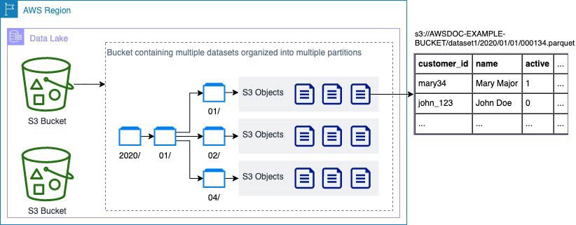
Most customers have their applications backed by various sql and nosql systems on prem and on cloud. Since the data is in various independent systems, customers struggle to derive meaningful info by combining data from all of these sources. Hence, customers create data lakes to bring their data in a single place.

Typically, a replication tool such as AWS Database Migration Service (AWS DMS) can replicate the data from your source systems to Amazon Simple Storage Service (Amazon S3). When the data is in Amazon S3, customers process it based on their requirements. A typical requirement is to sync the data in Amazon S3 with the updates on the source systems. Although it’s easy to apply updates on a relational database management system (RDBMS) that backs an online source application, it’s tough to apply this change data capture (CDC) process on your data lakes. Apache Hudi is a good way to solve this problem. Currently, you can use Hudi on Amazon EMR to create Hudi tables.

In this post, we use Apache Hudi to create tables in the AWS Glue Data Catalog using AWS Glue jobs. AWS Glue is a fully managed extract, transform, and load (ETL) service that makes it easy to prepare and load your data for analytics. This post enables you to take advantage of the serverless architecture of AWS Glue while upserting data in your data lake, hassle-free.

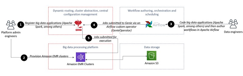
To write to Hudi tables using AWS Glue jobs, we use a JAR file created using open-source Apache Hudi. This JAR file is used as a dependency in the AWS Glue jobs created through the AWS CloudFormation template provided in this post. Steps to create the JAR file are included in the appendix.

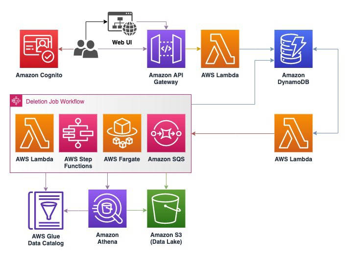
The following diagram illustrates the architecture the CloudFormation template implements.

Prerequisites

The CloudFormation template requires you to select an Amazon Elastic Compute Cloud (Amazon EC2) key pair. This key is configured on an EC2 instance that lives in the public subnet. We use this EC2 instance to get to the Aurora cluster that lives in the private subnet. Make sure you have a key in the Region where you deploy the template. If you don’t have one, you can create a new key pair.

Solution overview

The following are the high-level implementation steps:

  1. Create a CloudFormation stack using the provided template.
  2. Connect to the Amazon Aurora cluster used as a source for this post.
  3. Run InitLoad_TestStep1.sql, in the source Amazon Aurora cluster, to create a schema and a table.

AWS DMS replicates the data from the Aurora cluster to the raw S3 bucket. AWS DMS supports a variety of sources.
The CloudFormation stack creates an AWS Glue job (HudiJob) that is scheduled to run at a frequency set in the ScheduleToRunGlueJob parameter of the CloudFormation stack. This job reads the data from the raw S3 bucket, writes to the Curated S3 bucket, and creates a Hudi table in the Data Catalog. The job also creates an Amazon Redshift external schema in the Amazon Redshift cluster created by the CloudFormation stack.

  1. You can now query the Hudi table in Amazon Athena or Amazon Redshift. Visit Creating external tables for data managed in Apache Hudi or Considerations and Limitations to query Apache Hudi datasets in Amazon Athena for details.
  2. Run IncrementalUpdatesAndInserts_TestStep2.sql on the source Aurora cluster.

This incremental data is also replicated to the raw S3 bucket through AWS DMS. HudiJob picks up the incremental data, using AWS Glue bookmarks, and applies it to the Hudi table created earlier.

  1. You can now query the changed data.

Creating your CloudFormation stack

Click on the Launch Stack button to get started and provide the following parameters:

Parameter Description
VpcCIDR CIDR range for the VPC.
PrivateSubnet1CIDR CIDR range for the first private subnet.
PrivateSubnet2CIDR CIDR range for the second private subnet.
PublicSubnetCIDR CIDR range for the public subnet.
AuroraDBMasterUserPassword Primary user password for the Aurora cluster.
RedshiftDWMasterUserPassword Primary user password for the Amazon Redshift data warehouse.
KeyName The EC2 key pair to be configured in the EC2 instance on the public subnet. This EC2 instance is used to get to the Aurora cluster in the private subnet. Select the value from the dropdown.
ClientIPCIDR Your IP address in CIDR notation. The CloudFormation template creates a security group rule that grants ingress on port 22 to this IP address. On a Mac, you can run the following command to get your IP address: curl ipecho.net/plain ; echo /32
EC2ImageId The image ID used to create the EC2 instance in the public subnet to be a jump box to connect to the source Aurora cluster. If you supply your image ID, the template uses it to create the EC2 instance.
HudiStorageType This is used by the AWS Glue job to determine if you want to create a CoW or MoR storage type table. Enter MoR if you want to create MoR storage type tables.
ScheduleToRunGlueJob The AWS Glue job runs on a schedule to pick the new files and load to the curated bucket. This parameter sets the schedule of the job.
DMSBatchUnloadIntervalInSecs AWS DMS batches the inputs from the source and loads the output to the taw bucket. This parameter defines the frequency in which the data is loaded to the raw bucket.
GlueJobDPUs The number of DPUs that are assigned to the two AWS Glue jobs.

To simplify running the template, your account is given permissions on the key used to encrypt the resources in the CloudFormation template. You can restrict that to the role if desired.

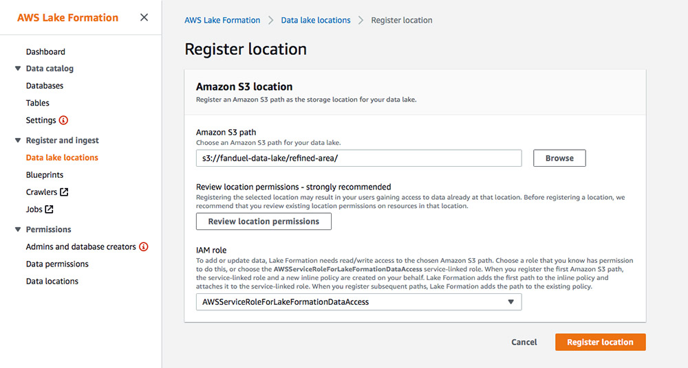
Granting Lake Formation permissions

AWS Lake Formation enables customers to set up fine grained access control for their Datalake. Detail steps to set up AWS Lake Formation can be found here.

Setting up AWS Lake Formation is out of scope for this post. However, if you have Lake Formation configured in the Region where you’re deploying this template, grant Create database permission to the LakeHouseExecuteGlueHudiJobRole role after the CloudFormation stack is successfully created.

This will ensure that you don’t get the following error while running your AWS Glue job.

org.apache.spark.sql.AnalysisException: org.apache.hadoop.hive.ql.metadata.HiveException: MetaException(message:Insufficient Lake Formation permission(s) on global_temp

Similarly grant Describe permission to the LakeHouseExecuteGlueHudiJobRole role on default database.

This will ensure that you don’t get the following error while running your AWS Glue job.

AnalysisException: 'java.lang.RuntimeException: MetaException(message:Unable to verify existence of default database: com.amazonaws.services.glue.model.AccessDeniedException: Insufficient Lake Formation permission(s) on default (Service: AWSGlue; Status Code: 400; Error Code: AccessDeniedException;

Connecting to source Aurora cluster

To connect to source Aurora cluster using SQL Workbench, complete the following steps:

  1. On SQL Workbench, under File, choose Connect window.

  1. Choose Manage Drivers.

  1. Choose PostgreSQL.
  2. For Library, use the driver JAR file.
  3. For Classname, enter org.postgresql.Driver.
  4. For Sample URL, enter jdbc:postgresql://host:port/name_of_database.

  1. Click the Create a new connection profile button.
  2. For Driver, choose your new PostgreSQL driver.
  3. For URL, enter lakehouse_source_db after port/.
  4. For Username, enter postgres.
  5. For Password, enter the same password that you used for the AuroraDBMasterUserPassword parameter while creating the CloudFormation stack.
  6. Choose SSH.
  7. On the Outputs tab of your CloudFormation stack, copy the IP address next to PublicIPOfEC2InstanceForTunnel and enter it for SSH hostname.
  8. For SSH port, enter 22.
  9. For Username, enter ec2-user.
  10. For Private key file, enter the private key for the public key chosen in the KeyName parameter of the CloudFormation stack.
  11. For Local port, enter any available local port number.
  12. On the Outputs tab of your stack, copy the value next to EndpointOfAuroraCluster and enter it for DB hostname.
  13. For DB port, enter 5432.
  14. Select Rewrite JDBC URL.


Checking the Rewrite JDBC URL checkbox will automatically feed in the value of host and port in the URL text box as shown below.

  1. Test the connection and make sure that you get a message that the connection was successful.


Troubleshooting

Complete the following steps if you receive this message: Could not initialize SSH tunnel: java.net.ConnectException: Operation timed out (Connection timed out)

  1. Go to your CloudFormation stack and search for LakeHouseSecurityGroup under Resources .
  2. Choose the link in the Physical ID.

  1. Select your security group.
  2. From the Actions menu, choose Edit inbound rules.

  1. Look for the rule with the description:Rule to allow connection from the SQL client to the EC2 instance used as jump box for SSH tunnel
  2. From the Source menu, choose My IP.
  3. Choose Save rules.

  1. Test the connection from your SQL Workbench again and make sure that you get a successful message.

Running the initial load script

You’re now ready to run the InitLoad_TestStep1.sql script to create some test data.

  1. Open InitLoad_TestStep1.sql in your SQL client and run it.

The output shows that 11 statements have been run.

AWS DMS replicates these inserts to your raw S3 bucket at the frequency set in the DMSBatchUnloadIntervalInSecs parameter of your CloudFormation stack.

  1. On the AWS DMS console, choose the lakehouse-aurora-src-to-raw-s3-tgt task:
  2. On the Table statistics tab, you should see the seven full load rows of employee_details have been replicated.

The lakehouse-aurora-src-to-raw-s3-tgt replication task has the following table mapping with transformation to add a schema name and a table name as additional columns:

{
   "rules":[
      {
         "rule-type":"selection",
         "rule-id":"1",
         "rule-name":"1",
         "object-locator":{
            "schema-name":"human_resources",
            "table-name":"%"
         },
         "rule-action":"include",
         "filters":[
            
         ]
      },
      {
         "rule-type":"transformation",
         "rule-id":"2",
         "rule-name":"2",
         "rule-target":"column",
         "object-locator":{
            "schema-name":"%",
            "table-name":"%"
         },
         "rule-action":"add-column",
         "value":"schema_name",
         "expression":"$SCHEMA_NAME_VAR",
         "data-type":{
            "type":"string",
            "length":50
         }
      },
      {
         "rule-type":"transformation",
         "rule-id":"3",
         "rule-name":"3",
         "rule-target":"column",
         "object-locator":{
            "schema-name":"%",
            "table-name":"%"
         },
         "rule-action":"add-column",
         "value":"table_name",
         "expression":"$TABLE_NAME_VAR",
         "data-type":{
            "type":"string",
            "length":50
         }
      }
   ]
}

These settings put the name of the source schema and table as two additional columns in the output Parquet file of AWS DMS.
These columns are used in the AWS Glue HudiJob to find out the tables that have new inserts, updates, or deletes.

  1. On the Resources tab of the CloudFormation stack, locate RawS3Bucket.
  2. Choose the Physical ID link.

  1. Navigate to human_resources/employee_details.

The LOAD00000001.parquet file is created under human_resources/employee_details. (The name of your raw bucket is different from the following screenshot).

You can also see the time of creation of this file. You should have at least one successful run of the AWS Glue job (HudiJob) after this time for the Hudi table to be created. The AWS Glue job is configured to load this data into the curated bucket at the frequency set in the ScheduleToRunGlueJob parameter of your CloudFormation stack. The default is 5 minutes.

AWS Glue job HudiJob

The following code is the script for HudiJob:

import sys
import os
import json

from pyspark.context import SparkContext
from pyspark.sql.session import SparkSession
from pyspark.sql.functions import concat, col, lit, to_timestamp

from awsglue.utils import getResolvedOptions
from awsglue.context import GlueContext
from awsglue.job import Job
from awsglue.dynamicframe import DynamicFrame

import boto3
from botocore.exceptions import ClientError

args = getResolvedOptions(sys.argv, ['JOB_NAME'])

spark = SparkSession.builder.config('spark.serializer','org.apache.spark.serializer.KryoSerializer').getOrCreate()
glueContext = GlueContext(spark.sparkContext)
job = Job(glueContext)
job.init(args['JOB_NAME'], args)
logger = glueContext.get_logger()

logger.info('Initialization.')
glueClient = boto3.client('glue')
ssmClient = boto3.client('ssm')
redshiftDataClient = boto3.client('redshift-data')

logger.info('Fetching configuration.')
region = os.environ['AWS_DEFAULT_REGION']

curatedS3BucketName = ssmClient.get_parameter(Name='lakehouse-curated-s3-bucket-name')['Parameter']['Value']
rawS3BucketName = ssmClient.get_parameter(Name='lakehouse-raw-s3-bucket-name')['Parameter']['Value']
hudiStorageType = ssmClient.get_parameter(Name='lakehouse-hudi-storage-type')['Parameter']['Value']

dropColumnList = ['db','table_name','Op']

logger.info('Getting list of schema.tables that have changed.')
changeTableListDyf = glueContext.create_dynamic_frame_from_options(connection_type = 's3', connection_options = {'paths': ['s3://'+rawS3BucketName], 'groupFiles': 'inPartition', 'recurse':True}, format = 'parquet', format_options={}, transformation_ctx = 'changeTableListDyf')

logger.info('Processing starts.')
if(changeTableListDyf.count() > 0):
    logger.info('Got new files to process.')
    changeTableList = changeTableListDyf.toDF().select('schema_name','table_name').distinct().rdd.map(lambda row : row.asDict()).collect()

    for dbName in set([d['schema_name'] for d in changeTableList]):
        spark.sql('CREATE DATABASE IF NOT EXISTS ' + dbName)
        redshiftDataClient.execute_statement(ClusterIdentifier='lakehouse-redshift-cluster', Database='lakehouse_dw', DbUser='rs_admin', Sql='CREATE EXTERNAL SCHEMA IF NOT EXISTS ' + dbName + ' FROM DATA CATALOG DATABASE \'' + dbName + '\' REGION \'' + region + '\' IAM_ROLE \'' + boto3.client('iam').get_role(RoleName='LakeHouseRedshiftGlueAccessRole')['Role']['Arn'] + '\'')

    for i in changeTableList:
        logger.info('Looping for ' + i['schema_name'] + '.' + i['table_name'])
        dbName = i['schema_name']
        tableNameCatalogCheck = ''
        tableName = i['table_name']
        if(hudiStorageType == 'MoR'):
            tableNameCatalogCheck = i['table_name'] + '_ro' #Assumption is that if _ro table exists then _rt table will also exist. Hence we are checking only for _ro.
        else:
            tableNameCatalogCheck = i['table_name'] #The default config in the CF template is CoW. So assumption is that if the user hasn't explicitly requested to create MoR storage type table then we will create CoW tables. Again, if the user overwrites the config with any value other than 'MoR' we will create CoW storage type tables.
        isTableExists = False
        isPrimaryKey = False
        isPartitionKey = False
        primaryKey = ''
        partitionKey = ''
        try:
            glueClient.get_table(DatabaseName=dbName,Name=tableNameCatalogCheck)
            isTableExists = True
            logger.info(dbName + '.' + tableNameCatalogCheck + ' exists.')
        except ClientError as e:
            if e.response['Error']['Code'] == 'EntityNotFoundException':
                isTableExists = False
                logger.info(dbName + '.' + tableNameCatalogCheck + ' does not exist. Table will be created.')
        try:
            table_config = json.loads(ssmClient.get_parameter(Name='lakehouse-table-' + dbName + '.' + tableName)['Parameter']['Value'])
            try:
                primaryKey = table_config['primaryKey']
                isPrimaryKey = True
                logger.info('Primary key:' + primaryKey)
            except KeyError as e:
                isPrimaryKey = False
                logger.info('Primary key not found. An append only glueparquet table will be created.')
            try:
                partitionKey = table_config['partitionKey']
                isPartitionKey = True
                logger.info('Partition key:' + partitionKey)
            except KeyError as e:
                isPartitionKey = False
                logger.info('Partition key not found. Partitions will not be created.')
        except ClientError as e:    
            if e.response['Error']['Code'] == 'ParameterNotFound':
                isPrimaryKey = False
                isPartitionKey = False
                logger.info('Config for ' + dbName + '.' + tableName + ' not found in parameter store. Non partitioned append only table will be created.')

        inputDyf = glueContext.create_dynamic_frame_from_options(connection_type = 's3', connection_options = {'paths': ['s3://' + rawS3BucketName + '/' + dbName + '/' + tableName], 'groupFiles': 'none', 'recurse':True}, format = 'parquet',transformation_ctx = tableName)
        
        inputDf = inputDyf.toDF().withColumn('update_ts_dms',to_timestamp(col('update_ts_dms')))
        
        targetPath = 's3://' + curatedS3BucketName + '/' + dbName + '/' + tableName

        morConfig = {'hoodie.datasource.write.storage.type': 'MERGE_ON_READ', 'hoodie.compact.inline': 'false', 'hoodie.compact.inline.max.delta.commits': 20, 'hoodie.parquet.small.file.limit': 0}

        commonConfig = {'className' : 'org.apache.hudi', 'hoodie.datasource.hive_sync.use_jdbc':'false', 'hoodie.datasource.write.precombine.field': 'update_ts_dms', 'hoodie.datasource.write.recordkey.field': primaryKey, 'hoodie.table.name': tableName, 'hoodie.consistency.check.enabled': 'true', 'hoodie.datasource.hive_sync.database': dbName, 'hoodie.datasource.hive_sync.table': tableName, 'hoodie.datasource.hive_sync.enable': 'true'}

        partitionDataConfig = {'hoodie.datasource.write.partitionpath.field': partitionKey, 'hoodie.datasource.hive_sync.partition_extractor_class': 'org.apache.hudi.hive.MultiPartKeysValueExtractor', 'hoodie.datasource.hive_sync.partition_fields': partitionKey}
                     
        unpartitionDataConfig = {'hoodie.datasource.hive_sync.partition_extractor_class': 'org.apache.hudi.hive.NonPartitionedExtractor', 'hoodie.datasource.write.keygenerator.class': 'org.apache.hudi.keygen.NonpartitionedKeyGenerator'}
        
        incrementalConfig = {'hoodie.upsert.shuffle.parallelism': 20, 'hoodie.datasource.write.operation': 'upsert', 'hoodie.cleaner.policy': 'KEEP_LATEST_COMMITS', 'hoodie.cleaner.commits.retained': 10}
        
        initLoadConfig = {'hoodie.bulkinsert.shuffle.parallelism': 3, 'hoodie.datasource.write.operation': 'bulk_insert'}
        
        deleteDataConfig = {'hoodie.datasource.write.payload.class': 'org.apache.hudi.common.model.EmptyHoodieRecordPayload'}

        if(hudiStorageType == 'MoR'):
            commonConfig = {**commonConfig, **morConfig}
            logger.info('MoR config appended to commonConfig.')
        
        combinedConf = {}

        if(isPrimaryKey):
            logger.info('Going the Hudi way.')
            if(isTableExists):
                logger.info('Incremental load.')
                outputDf = inputDf.filter("Op != 'D'").drop(*dropColumnList)
                if outputDf.count() > 0:
                    logger.info('Upserting data.')
                    if (isPartitionKey):
                        logger.info('Writing to partitioned Hudi table.')
                        outputDf = outputDf.withColumn(partitionKey,concat(lit(partitionKey+'='),col(partitionKey)))
                        combinedConf = {**commonConfig, **partitionDataConfig, **incrementalConfig}
                        outputDf.write.format('org.apache.hudi').options(**combinedConf).mode('Append').save(targetPath)
                    else:
                        logger.info('Writing to unpartitioned Hudi table.')
                        combinedConf = {**commonConfig, **unpartitionDataConfig, **incrementalConfig}
                        outputDf.write.format('org.apache.hudi').options(**combinedConf).mode('Append').save(targetPath)
                outputDf_deleted = inputDf.filter("Op = 'D'").drop(*dropColumnList)
                if outputDf_deleted.count() > 0:
                    logger.info('Some data got deleted.')
                    if (isPartitionKey):
                        logger.info('Deleting from partitioned Hudi table.')
                        outputDf_deleted = outputDf_deleted.withColumn(partitionKey,concat(lit(partitionKey+'='),col(partitionKey)))
                        combinedConf = {**commonConfig, **partitionDataConfig, **incrementalConfig, **deleteDataConfig}
                        outputDf_deleted.write.format('org.apache.hudi').options(**combinedConf).mode('Append').save(targetPath)
                    else:
                        logger.info('Deleting from unpartitioned Hudi table.')
                        combinedConf = {**commonConfig, **unpartitionDataConfig, **incrementalConfig, **deleteDataConfig}
                        outputDf_deleted.write.format('org.apache.hudi').options(**combinedConf).mode('Append').save(targetPath)
            else:
                outputDf = inputDf.drop(*dropColumnList)
                if outputDf.count() > 0:
                    logger.info('Inital load.')
                    if (isPartitionKey):
                        logger.info('Writing to partitioned Hudi table.')
                        outputDf = outputDf.withColumn(partitionKey,concat(lit(partitionKey+'='),col(partitionKey)))
                        combinedConf = {**commonConfig, **partitionDataConfig, **initLoadConfig}
                        outputDf.write.format('org.apache.hudi').options(**combinedConf).mode('Overwrite').save(targetPath)
                    else:
                        logger.info('Writing to unpartitioned Hudi table.')
                        combinedConf = {**commonConfig, **unpartitionDataConfig, **initLoadConfig}
                        outputDf.write.format('org.apache.hudi').options(**combinedConf).mode('Overwrite').save(targetPath)
        else:
            if (isPartitionKey):
                logger.info('Writing to partitioned glueparquet table.')
                sink = glueContext.getSink(connection_type = 's3', path= targetPath, enableUpdateCatalog = True, updateBehavior = 'UPDATE_IN_DATABASE', partitionKeys=[partitionKey])
            else:
                logger.info('Writing to unpartitioned glueparquet table.')
                sink = glueContext.getSink(connection_type = 's3', path= targetPath, enableUpdateCatalog = True, updateBehavior = 'UPDATE_IN_DATABASE')
            sink.setFormat('glueparquet')
            sink.setCatalogInfo(catalogDatabase = dbName, catalogTableName = tableName)
            outputDyf = DynamicFrame.fromDF(inputDf.drop(*dropColumnList), glueContext, 'outputDyf')
            sink.writeFrame(outputDyf)

job.commit()

Hudi tables need a primary key to perform upserts. Hudi tables can also be partitioned based on a certain key. We get the names of the primary key and the partition key from AWS Systems Manager Parameter Store.

The HudiJob script looks for an AWS Systems Manager Parameter with the naming format lakehouse-table-<schema_name>.<table_name>. It compares the name of the parameter with the name of the schema and table columns, added by AWS DMS, to get the primary key and the partition key for the Hudi table.

The CloudFormation template creates lakehouse-table-human_resources.employee_details AWS Systems Manager Parameter, as shown on the Resources tab.

If you choose the Physical ID link, you can locate the value of the AWS Systems Manager Parameter. The AWS Systems Manager Parameter has {"primaryKey": "emp_no", "partitionKey": "department"} value in it.

Because of the value in the lakehouse-table-human_resources.employee_details AWS Systems Manager Parameter, the AWS Glue script creates a human_resources.employee_details Hudi table partitioned on the department column for the employee_details table created in the source using the InitLoad_TestStep1.sql script. The HudiJob also uses the emp_no column as the primary key for upserts.

If you reuse this CloudFormation template and create your own table, you have to create an associated AWS Systems Manager Parameter with the naming convention lakehouse-table-<schema_name>.<table_name>. Keep in mind the following:

  • If you don’t create a parameter, the script creates an unpartitioned glueparquet append-only table.
  • If you create a parameter that only has the primaryKey part in the value, the script creates an unpartitioned Hudi table.
  • If you create a parameter that only has the partitionKey part in the value, the script creates a partitioned glueparquet append-only table.

If you have too many tables to replicate, you can also store the primary key and partition key configuration in Amazon DynamoDB or Amazon S3 and change the code accordingly.

In the InitLoad_TestStep1.sql script, replica identity for human_resources.employee_details table is set to full. This makes sure that AWS DMS transfers the full delete record to Amazon S3. Having this delete record is important for the HudiJob script to delete the record from the Hudi table. A full delete record from AWS DMS for the human_resources.employee_details table looks like the following:

{ "Op": "D", "update_ts_dms": "2020-10-25 07:57:48.589284", "emp_no": 3, "name": "Jeff", "department": "Finance", "city": "Tokyo", "salary": 55000, "schema_name": "human_resources", "table_name": "employee_details"}

The schema_name, and table_name columns are added by AWS DMS because of the task configuration shared previously.update_ts_dms has been set as the value for TimestampColumnName S3 setting in AWS DMS S3 Endpoint.Op is added by AWS DMS for cdc and it indicates source DB operations in migrated S3 data.

We also set spark.serializer in the script. This setting is required for Hudi.

In HudiJob script, you can also find a few Python dict that store various Hudi configuration properties. These configurations are just for demo purposes; you have to adjust them based on your workload. For more information about Hudi configurations, see Configurations.

HudiJob is scheduled to run every 5 minutes by default. The frequency is set by the ScheduleToRunGlueJob parameter of the CloudFormation template. Make sure that you successfully run HudiJob at least one time after the source data lands in the raw S3 bucket. The screenshot in Step 6 of Running the initial load script section confirms that AWS DMS put the LOAD00000001.parquet file in the raw bucket at 11:54:41 AM and following screenshot confirms that the job execution started at 11:55 AM.

The job creates a Hudi table in the AWS Glue Data Catalog (see the following screenshot). The table is partitioned on the department column.

Granting AWS Lake Formation permissions

If you have AWS Lake Formation enabled, make sure that you grant Select permission on the human_resources.employee_details table to the role/user used to run Athena query. Similarly, you also have to grant Select permission on the human_resources.employee_details table to the LakeHouseRedshiftGlueAccessRole role so you can query human_resources.employee_details in Amazon Redshift.

Grant Drop permission on the human_resources database to LakeHouseExecuteLambdaFnsRole so that the template can delete the database when you delete the template. Also, the CloudFormation template does not roll back any AWS Lake Formation grants or changes that are manually applied.

Granting access to KMS key

The curated S3 bucket is encrypted by lakehouse-key, which is an AWS Key Management Service (AWS KMS) customer managed key created by AWS CloudFormation template.

To run the query in Athena, you have to add the ARN of the role/user used to run the Athena query in the Allow use of the key section in the key policy.

This will ensure that you don’t get com.amazonaws.services.s3.model.AmazonS3Exception: Access Denied (Service: Amazon S3; Status Code: 403; Error Code: AccessDenied; error while running your Athena query.

You might not have to execute the above KMS policy change if you have kept the default of granting access to the AWS account and the role/user used to run Athena query has the necessary KMS related policies attached to it.

Confirming job completion

When HudiJob is complete, you can see the files in the curated bucket.

  1. On the Resources tab, search for CuratedS3Bucket.
  2. Choose the Physical ID link.

The following screenshot shows the timestamp on the initial load.

  1. Navigate to the department=Finance prefix and select the Parquet file.
  2. Choose Select from.
  1. For File format, select Parquet.
  2. Choose Show file preview.

You can see the value of the timestamp in the update_ts_dms column.

Querying the Hudi table

You can now query your data in Amazon Athena or Amazon Redshift.

Querying in Amazon Athena

Query the human_resources.employee_details table in Amazon Athena with the following code:

SELECT emp_no,
         name,
         city,
         salary,
         department,
         from_unixtime(update_ts_dms/1000000,'America/Los_Angeles') update_ts_dms_LA,
         from_unixtime(update_ts_dms/1000000,'UTC') update_ts_dms_UTC         
FROM "human_resources"."employee_details"
ORDER BY emp_no

The timestamp for all the records matches the timestamp in the update_ts_dms column in the earlier screenshot.

Querying in Redshift Spectrum

Read query your table in Redshift Spectrum for Apache Hudi support in Amazon Redshift.

  1. On the Amazon Redshift console, locate lakehouse-redshift-cluster.
  2. Choose Query cluster.

  1. For Database name, enter lakehouse_dw.
  2. For Database user, enter rs_admin.
  3. For Database password, enter the password that you used for the RedshiftDWMasterUserPassword parameter in the CloudFormation template.

  1. Enter the following query for the human_resources.employee_details table:
    SELECT emp_no,
             name,
             city,
             salary,
             department,
             (TIMESTAMP 'epoch' + update_ts_dms/1000000 * interval '1 second') AT TIME ZONE 'utc' AT TIME ZONE 'america/los_angeles' update_ts_dms_LA,
             (TIMESTAMP 'epoch' + update_ts_dms/1000000 * interval '1 second') AT TIME ZONE 'utc' update_ts_dms_UTC
    FROM human_resources.employee_details
    ORDER BY emp_no 

The following screenshot shows the query output.

Running the incremental load script

We now run the IncrementalUpdatesAndInserts_TestStep2.sql script. The output shows that 6 statements were run.

AWS DMS now shows that it has replicated the new incremental changes. The changes are replicated at a frequency set in DMSBatchUnloadIntervalInSecs parameter of the CloudFormation stack.

This creates another Parquet file in the raw S3 bucket.

The incremental updates are loaded into the Hudi table according to the chosen frequency to run the job (the ScheduleToRunGlueJob parameter). The HudiJobscript uses job bookmarks to find out the incremental load so it only processes the new files brought in through AWS DMS.

Confirming job completion

Make sure that HudiJob runs successfully at least one time after the incremental file arrives in the raw bucket. The previous screenshot shows that the incremental file arrived in the raw bucket at 1:18:38 PM and the following screenshot shows that the job started at 1:20 PM.

Querying the changed data

You can now check the table in Athena and Amazon Redshift. Both results show that emp_no 3 is deleted, 8 and 9 have been added, and 2 and 5 have been updated.

The following screenshot shows the results in Athena.

The following screenshot shows the results in Redshift Spectrum.

AWS Glue Job HudiMoRCompactionJob

The CloudFormation template also deploys the AWS Glue job HudiMoRCompactionJob. This job is not scheduled; you only use it if you choose the MoR storage type. To execute the pipe for MoR storage type instead of CoW storage type, delete the CloudFormation stack and create it again. After creation, replace CoW in lakehouse-hudi-storage-type AWS Systems Manager Parameter with MoR.

If you use MoR storage type, the incremental updates are stored in log files. You can’t see the updates in the _ro (read optimized) view, but can see them in the _rt view. Amazon Athena documentation and Amazon Redshift documentation gives more details about support and considerations for Apache Hudi.

To see the incremental data in the _ro view, run the HudiMoRCompactionJob job. For more information about Hudi storage types and views, see Hudi Dataset Storage Types and Storage Types & Views. The following code is an example of the CLI command used to run HudiMoRCompactionJob job:

aws glue start-job-run --job-name HudiMoRCompactionJob --arguments="--DB_NAME=human_resources","--TABLE_NAME=employee_details","--IS_PARTITIONED=true"

You can decide on the frequency of running this job. You don’t have to run the job immediately after the HudiJob. You should run this job when you want the data to be available in the _ro view. You have to pass the schema name and the table name to this script so it knows the table to compact.

Additional considerations

The JAR file we use in this post has not been tested for AWS Glue streaming jobs. Additionally, there are some hardcoded Hudi options in the HudiJob script. These options are set for the sample table that we create for this post. Update the options based on your workload. 

Conclusion

In this post, we created AWS Glue 2.0 jobs that moved the source upserts and deletes into Hudi tables. The code creates tables in the AWS GLue Data Catalog and updates partitions so you don’t have to run the crawlers to update them.

This post simplified your LakeHouse code base by giving you the benefits of Apache Hudi along with serverless AWS Glue. We also showed how to create an source to LakeHouse replication system using AWS Glue, AWS DMS, and Amazon Redshift with minimum overhead.


Appendix

We can write to Hudi tables because of the hudi-spark.jar file that we downloaded to our DependentJarsAndTempS3Bucket S3 bucket with the CloudFormation template. The path to this file is added as a dependency in both the AWS Glue jobs. This file is based on open-source Hudi. To create the JAR file, complete the following steps:

  1. Get Hudi 0.5.3 and unzip it using the following code:
    wget https://github.com/apache/hudi/archive/release-0.5.3.zip
    unzip hudi-release-0.5.3.zip

  2. Edit Hudi pom.xml:
    vi hudi-release-0.5.3/pom.xml

    1. Remove the following code to make the build process faster:
      <module>packaging/hudi-hadoop-mr-bundle</module>
      <module>packaging/hudi-hive-bundle</module>
      <module>packaging/hudi-presto-bundle</module>
      <module>packaging/hudi-utilities-bundle</module>
      <module>packaging/hudi-timeline-server-bundle</module>
      <module>docker/hoodie/hadoop</module>
      <module>hudi-integ-test</module>

    2. Change the versions of all three dependencies of httpcomponents to 4.4.1. The following is the original code:
      <!-- Httpcomponents -->
            <dependency>
              <groupId>org.apache.httpcomponents</groupId>
              <artifactId>fluent-hc</artifactId>
              <version>4.3.2</version>
            </dependency>
            <dependency>
              <groupId>org.apache.httpcomponents</groupId>
              <artifactId>httpcore</artifactId>
              <version>4.3.2</version>
            </dependency>
            <dependency>
              <groupId>org.apache.httpcomponents</groupId>
              <artifactId>httpclient</artifactId>
              <version>4.3.6</version>
            </dependency>

      The following is the replacement code:

      <!-- Httpcomponents -->
            <dependency>
              <groupId>org.apache.httpcomponents</groupId>
              <artifactId>fluent-hc</artifactId>
              <version>4.4.1</version>
            </dependency>
            <dependency>
              <groupId>org.apache.httpcomponents</groupId>
              <artifactId>httpcore</artifactId>
              <version>4.4.1</version>
            </dependency>
            <dependency>
              <groupId>org.apache.httpcomponents</groupId>
              <artifactId>httpclient</artifactId>
              <version>4.4.1</version>
            </dependency>

  3. Build the JAR file:
    mvn clean package -DskipTests -DskipITs -f <Full path of the hudi-release-0.5.3 dir>

  4. You can now get the JAR from the following location:
hudi-release-0.5.3/packaging/hudi-spark-bundle/target/hudi-spark-bundle_2.11-0.5.3-rc2.jar

The other JAR dependency used in the AWS Glue jobs is spark-avro_2.11-2.4.4.jar.


About the Author

Vishal Pathak is a Data Lab Solutions Architect at AWS. Vishal works with the customers on their use cases, architects a solution to solve their business problems and helps the customers build an scalable prototype. Prior to his journey in AWS, Vishal helped customers implement BI, DW and DataLake projects in US and Australia.

Getting started with RPA using AWS Step Functions and Amazon Textract

Post Syndicated from James Beswick original https://aws.amazon.com/blogs/compute/getting-started-with-rpa-using-aws-step-functions-and-amazon-textract/

This post is courtesy of Joe Tringali, Solutions Architect.

Many organizations are using robotic process automation (RPA) to automate workflow, back-office processes that are labor-intensive. RPA, as software bots, can often handle many of these activities. Often RPA workflows contain repetitive manual tasks that must be done by humans, such as viewing invoices to find payment details.

AWS Step Functions is a serverless function orchestrator and workflow automation tool. Amazon Textract is a fully managed machine learning service that automatically extracts text and data from scanned documents. Combining these services, you can create an RPA bot to automate the workflow and enable employees to handle more complex tasks.

In this post, I show how you can use Step Functions and Amazon Textract to build a workflow that enables the processing of invoices. Download the code for this solution from https://github.com/aws-samples/aws-step-functions-rpa.

Overview

The following serverless architecture can process scanned invoices in PDF or image formats for submitting payment information to a database.

Example architecture
To implement this architecture, I use single-purpose Lambda functions and Step Functions to build the workflow:

  1. Invoices are scanned and loaded into an Amazon Simple Storage Service (S3) bucket.
  2. The loading of an invoice into Amazon S3 triggers an AWS Lambda function to be invoked.
  3. The Lambda function starts an asynchronous Amazon Textract job to analyze the text and data of the scanned invoice.
  4. The Amazon Textract job publishes a completion notification message with a status of “SUCCEEDED” or “FAILED” to an Amazon Simple Notification Service (SNS) topic.
  5. SNS sends the message to an Amazon Simple Queue Service (SQS) queue that is subscribed to the SNS topic.
  6. The message in the SQS queue triggers another Lambda function.
  7. The Lambda function initiates a Step Functions state machine to process the results of the Amazon Textract job.
  8. For an Amazon Textract job that completes successfully, a Lambda function saves the document analysis into an Amazon S3 bucket.
  9. The loading of the document analysis to Amazon S3 triggers another Lambda function.
  10. The Lambda function retrieves the text and data of the scanned invoice to find the payment information. It writes an item to an Amazon DynamoDB table with a status indicating if the invoice can be processed.
  11. If the DynamoDB item contains the payment information, another Lambda function is invoked.
  12. The Lambda function archives the processed invoice into another S3 bucket.
  13. If the DynamoDB item does not contain the payment information, a message is published to an Amazon SNS topic requesting that the invoice be reviewed.

Amazon Textract can extract information from the various invoice images and associate labels with the data. You must then handle the various labels that different invoices may associate with the payee name, due date, and payment amount.

Determining payee name, due date and payment amount

After the document analysis has been saved to S3, a Lambda function retrieves the text and data of the scanned invoice to find the information needed for payment. However, invoices can use a variety of labels for the same piece of data, such a payment’s due date.

In the example invoices included with this blog, the payment’s due date is associated with the labels “Pay On or Before”, “Payment Due Date” and “Payment Due”. Payment amounts can also have different labels, such as “Total Due”, “New Balance Total”, “Total Current Charges”, and “Please Pay”. To address this, I use a series of helper functions in the app.py file in the process_document_analysis folder of the GitHub repo.

In app.py, there is the following get_ky_map helper function:

def get_kv_map(blocks):
    key_map = {}
    value_map = {}
    block_map = {}
    for block in blocks:
        block_id = block['Id']
        block_map[block_id] = block
        if block['BlockType'] == "KEY_VALUE_SET":
            if 'KEY' in block['EntityTypes']:
                key_map[block_id] = block
            else:
                value_map[block_id] = block
    return key_map, value_map, block_map

The get_kv_map function is invoked by the Lambda function handler. It iterates over the “Blocks” element of the document analysis produced by Amazon Textract to create dictionaries of keys (labels) and values (data) associated with each block identified by Amazon Textract. It then invokes the following get_kv_relationship helper function:

def get_kv_relationship(key_map, value_map, block_map):
    kvs = {}
    for block_id, key_block in key_map.items():
        value_block = find_value_block(key_block, value_map)
        key = get_text(key_block, block_map)
        val = get_text(value_block, block_map)
        kvs[key] = val
    return kvs

The get_kv_relationship function merges the key and value dictionaries produced by the get_kv_map function to create a single Python key value dictionary where labels are the keys to the dictionary and the invoice’s data are the values. The handler then invokes the following get_line_list helper function:

def get_line_list(blocks):
    line_list = []
    for block in blocks:
        if block['BlockType'] == "LINE":
            if 'Text' in block: 
                line_list.append(block["Text"])
    return line_list

Extracting payee names is more complex because the data may not be labeled. The payee may often differ from the entity sending the invoice. With the Amazon Textract analysis in a format more easily consumable by Python, I use the following get_payee_name helper function to parse and extract the payee:

def get_payee_name(lines):
    payee_name = ""
    payable_to = "payable to"
    payee_lines = [line for line in lines if payable_to in line.lower()]
    if len(payee_lines) > 0:
        payee_line = payee_lines[0]
        payee_line = payee_line.strip()
        pos = payee_line.lower().find(payable_to)
        if pos > -1:
            payee_line = payee_line[pos + len(payable_to):]
            if payee_line[0:1] == ':':
                payee_line = payee_line[1:]
            payee_name = payee_line.strip()
    return payee_name

The get_amount helper function searches the key value dictionary produced by the get_kv_relationship function to retrieve the payment amount:

def get_amount(kvs, lines):
    amount = None
    amounts = [search_value(kvs, amount_tag) for amount_tag in amount_tags if search_value(kvs, amount_tag) is not None]
    if len(amounts) > 0:
        amount = amounts[0]
    else:
        for idx, line in enumerate(lines):
            if line.lower() in amount_tags:
                amount = lines[idx + 1]
                break
    if amount is not None:
        amount = amount.strip()
        if amount[0:1] == '$':
            amount = amount[1:]
    return amount

The amount_tags variable contains a list of possible labels associated with the payment amount:

amount_tags = ["total due", "new balance total", "total current charges", "please pay"]

Similarly, the get_due_date helper function searches the key value dictionary produced by the get_kv_relationship function to retrieve the payment due date:

def get_due_date(kvs):
    due_date = None
    due_dates = [search_value(kvs, due_date_tag) for due_date_tag in due_date_tags if search_value(kvs, due_date_tag) is not None]
    if len(due_dates) > 0:
        due_date = due_dates[0]
    if due_date is not None:
        date_parts = due_date.split('/')
        if len(date_parts) == 3:
            due_date = datetime(int(date_parts[2]), int(date_parts[0]), int(date_parts[1])).isoformat()
        else:
            date_parts = [date_part for date_part in re.split("\s+|,", due_date) if len(date_part) > 0]
            if len(date_parts) == 3:
                datetime_object = datetime.strptime(date_parts[0], "%b")
                month_number = datetime_object.month
                due_date = datetime(int(date_parts[2]), int(month_number), int(date_parts[1])).isoformat()
    else:
        due_date = datetime.now().isoformat()
    return due_date

The due_date_tag contains a list of possible labels associated with the payment due:

due_date_tags = ["pay on or before", "payment due date", "payment due"]

If all required elements needed to issue a payment are found, it adds an item to the DynamoDB table with a status attribute of “Approved for Payment”. If the Lambda function cannot determine the value of one or more required elements, it adds an item to the DynamoDB table with a status attribute of “Pending Review”.

Payment Processing

If the item in the DynamoDB table is marked “Approved for Payment”, the processed invoice is archived. If the item’s status attribute is marked “Pending Review”, an SNS message is published to an SNS Pending Review topic. You can subscribe to this topic so that you can add additional labels to the Python code for determining payment due dates and payment amounts.

Note that the Lambda functions are single-purpose functions, and all workflow logic is contained in the Step Functions state machine. This diagram shows the various tasks (states) of a successful workflow.

State machine workflow

For more information about this solution, download the code from the GitHub repo (https://github.com/aws-samples/aws-step-functions-rpa).

Prerequisites

Before deploying the solution, you must install the following prerequisites:

  1. Python.
  2. AWS Command Line Interface (AWS CLI) – for instructions, see Installing the AWS CLI.
  3. AWS Serverless Application Model Command Line Interface (AWS SAM CLI) – for instructions, see Installing the AWS SAM CLI.

Deploying the solution

The solution creates the following S3 buckets with names suffixed by your AWS account ID to prevent a global namespace collision of your S3 bucket names:

  • scanned-invoices-<YOUR AWS ACCOUNT ID>
  • invoice-analyses-<YOUR AWS ACCOUNT ID>
  • processed-invoices-<YOUR AWS ACCOUNT ID>

The following steps deploy the example solution in your AWS account. The solution deploys several components including a Step Functions state machine, Lambda functions, S3 buckets, a DynamoDB table for payment information, and SNS topics.

AWS CloudFormation requires an S3 bucket and stack name for deploying the solution. To deploy:

  1. Download code from GitHub repo (https://github.com/aws-samples/aws-step-functions-rpa).
  2. Run the following command to build the artifacts locally on your workstation:sam build
  3. Run the following command to create a CloudFormation stack and deploy your resources:sam deploy --guided --capabilities CAPABILITY_NAMED_IAM

Monitor the progress and wait for the completion of the stack creation process from the AWS CloudFormation console before proceeding.

Testing the solution

To test the solution, upload the PDF test invoices to the S3 bucket named scanned-invoices-<YOUR AWS ACCOUNT ID>.

A Step Functions state machine with the name <YOUR STACK NAME>-ProcessedScannedInvoiceWorkflow runs the workflow. Amazon Textract document analyses are stored in the S3 bucket named invoice-analyses-<YOUR AWS ACCOUNT ID>, and processed invoices are stored in the S3 bucket named processed-invoices-<YOUR AWS ACCOUNT ID>. Processed payments are found in the DynamoDB table named <YOUR STACK NAME>-invoices.

You can monitor the status of the workflows from the Step Functions console. Upon completion of the workflow executions, review the items added to DynamoDB from the Amazon DynamoDB console.

Cleanup

To avoid ongoing charges for any resources you created in this blog post, delete the stack:

  1. Empty the three S3 buckets created during deployment using the S3 console:
    – scanned-invoices-<YOUR AWS ACCOUNT ID>
    – invoice-analyses-<YOUR AWS ACCOUNT ID>
    – processed-invoices-<YOUR AWS ACCOUNT ID>
  2. Delete the CloudFormation stack created during deployment using the CloudFormation console.

Conclusion

In this post, I showed you how to use a Step Functions state machine and Amazon Textract to automatically extract data from a scanned invoice. This eliminates the need for a person to perform the manual step of reviewing an invoice to find payment information to be fed into a backend system. By replacing the manual steps of a workflow with automation, an organization can free up their human workforce to handle more value-added tasks.

To learn more, visit AWS Step Functions and Amazon Textract for more information. For more serverless learning resources, visit https://serverlessland.com.


Using AWS Lambda extensions to send logs to custom destinations

Post Syndicated from Julian Wood original https://aws.amazon.com/blogs/compute/using-aws-lambda-extensions-to-send-logs-to-custom-destinations/

You can now send logs from AWS Lambda functions directly to a destination of your choice using AWS Lambda Extensions. Lambda Extensions are a new way for monitoring, observability, security, and governance tools to easily integrate with AWS Lambda. For more information, see “Introducing AWS Lambda Extensions – In preview”.

To help you troubleshoot failures in Lambda functions, AWS Lambda automatically captures and streams logs to Amazon CloudWatch Logs. This stream contains the logs that your function code and extensions generate, in addition to logs the Lambda service generates as part of the function invocation.

Previously, to send logs to a custom destination, you typically configure and operate a CloudWatch Log Group subscription. A different Lambda function forwards logs to the destination of your choice.

Logging tools, running as Lambda extensions, can now receive log streams directly from within the Lambda execution environment, and send them to any destination. This makes it even easier for you to use your preferred extensions for diagnostics.

Today, you can use extensions to send logs to Coralogix, Datadog, Honeycomb, Lumigo, New Relic, and Sumo Logic.

Overview

To receive logs, extensions subscribe using the new Lambda Logs API.

Lambda Logs API

Lambda Logs API

The Lambda service then streams the logs directly to the extension. The extension can then process, filter, and route them to any preferred destination. Lambda still sends the logs to CloudWatch Logs.

You deploy extensions, including ones that use the Logs API, as Lambda layers, with the AWS Management Console and AWS Command Line Interface (AWS CLI). You can also use infrastructure as code tools such as AWS CloudFormation, the AWS Serverless Application Model (AWS SAM), Serverless Framework, and Terraform.

Logging extensions from AWS Lambda Ready Partners and AWS Partners available at launch

Today, you can use logging extensions with the following tools:

  • The Datadog extension now makes it easier than ever to collect your serverless application logs for visualization, analysis, and archival. Paired with Datadog’s AWS integration, end-to-end distributed tracing, and real-time enhanced AWS Lambda metrics, you can proactively detect and resolve serverless issues at any scale.
  • Lumigo provides monitoring and debugging for modern cloud applications. With the open source extension from Lumigo, you can send Lambda function logs directly to an S3 bucket, unlocking new post processing use cases.
  • New Relic enables you to efficiently monitor, troubleshoot, and optimize your Lambda functions. New Relic’s extension allows you send your Lambda service platform logs directly to New Relic’s unified observability platform, allowing you to quickly visualize data with minimal latency and cost.
  • Coralogix is a log analytics and cloud security platform that empowers thousands of companies to improve security and accelerate software delivery, allowing you to get deep insights without paying for the noise. Coralogix can now read Lambda function logs and metrics directly, without using Cloudwatch or S3, reducing the latency, and cost of observability.
  • Honeycomb is a powerful observability tool that helps you debug your entire production app stack. Honeycomb’s extension decreases the overhead, latency, and cost of sending events to the Honeycomb service, while increasing reliability.
  • The Sumo Logic extension enables you to get instant visibility into the health and performance of your mission-critical applications using AWS Lambda. With this extension and Sumo Logic’s continuous intelligence platform, you can now ensure that all your Lambda functions are running as expected, by analyzing function, platform, and extension logs to quickly identify and remediate errors and exceptions.

You can also build and use your own logging extensions to integrate your organization’s tooling.

Showing a logging extension to send logs directly to S3

This demo shows an example of using a simple logging extension to send logs to Amazon Simple Storage Service (S3).

To set up the example, visit the GitHub repo and follow the instructions in the README.md file.

The example extension runs a local HTTP endpoint listening for HTTP POST events. Lambda delivers log batches to this endpoint. The example creates an S3 bucket to store the logs. A Lambda function is configured with an environment variable to specify the S3 bucket name. Lambda streams the logs to the extension. The extension copies the logs to the S3 bucket.

Lambda environment variable specifying S3 bucket

Lambda environment variable specifying S3 bucket

The extension uses the Extensions API to register for INVOKE and SHUTDOWN events. The extension, using the Logs API, then subscribes to receive platform and function logs, but not extension logs.

As the example is an asynchronous system, logs for one invoke may be processed during the next invocation. Logs for the last invoke may be processed during the SHUTDOWN event.

Testing the function from the Lambda console, Lambda sends logs to CloudWatch Logs. The logs stream shows logs from the platform, function, and extension.

Lambda logs visible in CloudWatch Logs

Lambda logs visible in CloudWatch Logs

The logging extension also receives the log stream directly from Lambda, and copies the logs to S3.

Browsing to the S3 bucket, the log files are available.

S3 bucket containing copied logs

S3 bucket containing copied logs.

Downloading the file shows the log lines. The log contains the same platform and function logs, but not the extension logs, as specified during the subscription.

[{'time': '2020-11-12T14:55:06.560Z', 'type': 'platform.start', 'record': {'requestId': '49e64413-fd42-47ef-b130-6fd16f30148d', 'version': '$LATEST'}},
{'time': '2020-11-12T14:55:06.774Z', 'type': 'platform.logsSubscription', 'record': {'name': 'logs_api_http_extension.py', 'state': 'Subscribed', 'types': ['platform', 'function']}},
{'time': '2020-11-12T14:55:06.774Z', 'type': 'platform.extension', 'record': {'name': 'logs_api_http_extension.py', 'state': 'Ready', 'events': ['INVOKE', 'SHUTDOWN']}},
{'time': '2020-11-12T14:55:06.776Z', 'type': 'function', 'record': 'Function: Logging something which logging extension will send to S3\n'}, {'time': '2020-11-12T14:55:06.780Z', 'type': 'platform.end', 'record': {'requestId': '49e64413-fd42-47ef-b130-6fd16f30148d'}}, {'time': '2020-11-12T14:55:06.780Z', 'type': 'platform.report', 'record': {'requestId': '49e64413-fd42-47ef-b130-6fd16f30148d', 'metrics': {'durationMs': 4.96, 'billedDurationMs': 100, 'memorySizeMB': 128, 'maxMemoryUsedMB': 87, 'initDurationMs': 792.41}, 'tracing': {'type': 'X-Amzn-Trace-Id', 'value': 'Root=1-5fad4cc9-70259536495de84a2a6282cd;Parent=67286c49275ac0ad;Sampled=1'}}}]

Lambda has sent specific logs directly to the subscribed extension. The extension has then copied them directly to S3.

For more example log extensions, see the Github repository.

How do extensions receive logs?

Extensions start a local listener endpoint to receive the logs using one of the following protocols:

  1. TCP – Logs are delivered to a TCP port in Newline delimited JSON format (NDJSON).
  2. HTTP – Logs are delivered to a local HTTP endpoint through PUT or POST, as an array of records in JSON format. http://sandbox:${PORT}/${PATH}. The $PATH parameter is optional.

AWS recommends using an HTTP endpoint over TCP because HTTP tracks successful delivery of the log messages to the local endpoint that the extension sets up.

Once the endpoint is running, extensions use the Logs API to subscribe to any of three different logs streams:

  • Function logs that are generated by the Lambda function.
  • Lambda service platform logs (such as the START, END, and REPORT logs in CloudWatch Logs).
  • Extension logs that are generated by extension code.

The Lambda service then sends logs to endpoint subscribers inside of the execution environment only.

Even if an extension subscribes to one or more log streams, Lambda continues to send all logs to CloudWatch.

Performance considerations

Extensions share resources with the function, such as CPU, memory, disk storage, and environment variables. They also share permissions, using the same AWS Identity and Access Management (IAM) role as the function.

Log subscriptions consume memory resources as each subscription opens a new memory buffer to store the logs. This memory usage counts towards memory consumed within the Lambda execution environment.

For more information on resources, security and performance with extensions, see “Introducing AWS Lambda Extensions – In preview”.

What happens if Lambda cannot deliver logs to an extension?

The Lambda service stores logs before sending to CloudWatch Logs and any subscribed extensions. If Lambda cannot deliver logs to the extension, it automatically retries with backoff. If the log subscriber crashes, Lambda restarts the execution environment. The logs extension re-subscribes, and continues to receive logs.

When using an HTTP endpoint, Lambda continues to deliver logs from the last acknowledged delivery. With TCP, the extension may lose logs if an extension or the execution environment fails.

The Lambda service buffers logs in memory before delivery. The buffer size is proportional to the buffering configuration used in the subscription request. If an extension cannot process the incoming logs quickly enough, the buffer fills up. To reduce the likelihood of an out of memory event due to a slow extension, the Lambda service drops records and adds a platform.logsDropped log record to the affected extension to indicate the number of dropped records.

Disabling logging to CloudWatch Logs

Lambda continues to send logs to CloudWatch Logs even if extensions subscribe to the logs stream.

To disable logging to CloudWatch Logs for a particular function, you can amend the Lambda execution role to remove access to CloudWatch Logs.

{
"Version": "2012-10-17",
"Statement": [
    {
        "Effect": "Deny",
        "Action": [
            "logs:CreateLogGroup",
            "logs:CreateLogStream",
            "logs:PutLogEvents"
        ],
        "Resource": [
            "arn:aws:logs:*:*:*"
        ]
    }
  ]
}

Logs are no longer delivered to CloudWatch Logs for functions using this role, but are still streamed to subscribed extensions. You are no longer billed for CloudWatch logging for these functions.

Pricing

Logging extensions, like other extensions, share the same billing model as Lambda functions. When using Lambda functions with extensions, you pay for requests served and the combined compute time used to run your code and all extensions, in 100 ms increments. To learn more about the billing for extensions, visit the Lambda FAQs page.

Conclusion

Lambda extensions enable you to extend the Lambda service to more easily integrate with your favorite tools for monitoring, observability, security, and governance.

Extensions can now subscribe to receive log streams directly from the Lambda service, in addition to CloudWatch Logs. Today, you can install a number of available logging extensions from AWS Lambda Ready Partners and AWS Partners. Extensions make it easier to use your existing tools with your serverless applications.

To try the S3 demo logging extension, follow the instructions in the README.md file in the GitHub repository.

Extensions are now available in preview in all commercial regions other than the China regions.

For more serverless learning resources, visit https://serverlessland.com.

New – Export Amazon DynamoDB Table Data to Your Data Lake in Amazon S3, No Code Writing Required

Post Syndicated from Alex Casalboni original https://aws.amazon.com/blogs/aws/new-export-amazon-dynamodb-table-data-to-data-lake-amazon-s3/

Hundreds of thousands of AWS customers have chosen Amazon DynamoDB for mission-critical workloads since its launch in 2012. DynamoDB is a nonrelational managed database that allows you to store a virtually infinite amount of data and retrieve it with single-digit-millisecond performance at any scale. To get the most value out of this data, customers had […]

S3 Intelligent-Tiering Adds Archive Access Tiers

Post Syndicated from Marcia Villalba original https://aws.amazon.com/blogs/aws/s3-intelligent-tiering-adds-archive-access-tiers/

We launched S3 Intelligent-Tiering two years ago, which added the capability to take advantage of S3 without needing to have a deep understanding of your data access patterns. Today we are launching two new optimizations for S3 Intelligent-Tiering that will automatically archive objects that are rarely accessed. These new optimizations will reduce the amount of […]

Handling data erasure requests in your data lake with Amazon S3 Find and Forget

Post Syndicated from Chris Deigan original https://aws.amazon.com/blogs/big-data/handling-data-erasure-requests-in-your-data-lake-with-amazon-s3-find-and-forget/

Data lakes are a popular choice for organizations to store data around their business activities. Best practice design of data lakes impose that data is immutable once stored, but new regulations such as the European General Data Protection Regulation (GDPR), California Consumer Privacy Act (CCPA), and others have created new obligations that operators now need to be able to erase private data from their data lake when requested.

When asked to erase an individual’s private data, as a data lake operator you have to find all the objects in your Amazon Simple Storage Service (Amazon S3) buckets that contain data relating to that individual. This can be complex because data lakes contain many S3 objects (each of which may contain multiple rows), as shown in the following diagram. You often can’t predict which objects contain data relating to an individual, so you need to check each object. For example, if the user mary34 asks to be removed, you need to check each object to determine if it contains data relating to mary34. This is the first challenge operators face: identifying which objects contain data of interest.

After you identify objects containing data of interest, you face a second challenge: you need to retrieve the object from the S3 bucket, remove relevant rows from the file, put a new version of the object into S3, and make sure you delete any older versions.

Locating and removing data manually can be time-consuming and prone to mistakes, considering the large number of objects typically in data lakes.

Amazon S3 Find and Forget solves these challenges with ready-to-use automations. It allows you to remove records from data lakes of any size that are in AWS Glue Data Catalog. The solution includes a web user interface that you can use and an API that you can use to integrate with your own applications.

Solution overview

Amazon S3 Find and Forget enables you to find and delete records automatically in data lakes on Amazon S3. Using the solution, you can:

  • Define which tables from your AWS Glue Data Catalog contain data you want to erase
  • Manage a queue of identifiers (such as unique customer identifiers) to erase
  • Erase rows from your data lake matching the queued record identifiers
  • Access a log of all actions taken by the solution

You can use Amazon S3 Find and Forget to work with data lakes stored on Amazon S3 in a supported file format.

The solution is developed and distributed as open-source software that you deploy and run inside your own AWS account. When deploying this solution, you only pay for the AWS services consumed to run it. We recommend reviewing the Cost Estimate guide and creating Amazon CloudWatch Billing Alarms to monitor charges before deploying the solution in your own account.

When you handle requests to remove data, you add the identifiers through the web interface or API to a Deletion Queue. The identifiers remain in the queue until you start a Deletion Job. The Deletion Job processes the queue and removes matching rows from objects in your data lake.

Where your requirements allow it, batching deletions can provide significant cost savings by minimizing the number of times the data lake needs to be re-scanned and processed. For example, you could start a Deletion Job once a week to process all requests received in the preceding week.

Solution demonstration

This section provides a demonstration of using Amazon S3 Find and Forget’s main features. To deploy the solution in your own account, refer to the User Guide.

For this demonstration, I have prepared in advance:

The first step is to deploy the solution using AWS CloudFormation by following the instructions in the User Guide. The CloudFormation stack can take 20-30 minutes to deploy depending on the options chosen when deploying.

Once deployed, I visit the web user interface by going to the address in the WebUIUrl CloudFormation stack output. Using a temporary password emailed to the address I provided in my CloudFormation parameters, I login and set a password for future use. I then see a dashboard with some base metrics for my Amazon S3 Find and Forget deployment:

I now need to create a Data Mapper so that Amazon S3 Find and Forget can find my data lake. To do this, I select Data Mappers, then Create Data Mapper:

On this screen, I give my Data Mapper a name, choose the AWS Glue database and table in my account that I want to operate on, and the columns that I want my deletions to match. In this demonstration, I’m using a copy of the Amazon Customer Reviews Dataset that I copied to my own S3 bucket. I’ll be using the customer_id column to remove data. In the dataset, this field contains a unique identifier for each customer who has created a product review.

I then specify the IAM role to be used when modifying the objects in S3. I also choose whether I want the old S3 object versions to be deleted for me. I can turn this off if I want to implement my own strategy to manage deleting old object versions, such as by using S3 lifecycle policies.

After choosing Create Data Mapper the Data Mapper is created, and I am prompted to grant permissions for S3 Find and Forget to operate in my bucket. In the Data Mapper list, I select my new Data Mapper, then choose Generate Access Policies. The interface displays a sample bucket policy that I copy and paste into the bucket policy for my S3 bucket in the AWS Management Console.

With the Data Mapper set up, I’m now able to add the customers who have requested to have their data deleted to the Deletion Queue. Using their Customer IDs, I go to the Deletion Queue section and select Add Match to the Deletion Queue.

I’ve chosen to delete from all the available Data Mappers, but I can also choose specific ones. Once I’ve added my matches, I can see a list of them on Deletion Queue page:

I can now run a deletion job that will cause the matches to be deleted from the data lake. To do this, I select Deletion Jobs then Start a Deletion Job.

After a few minutes the Deletion Job completes, and I can see metrics collected during the job including that the job took just over two-and-a-half minutes:

There is an Export to JSON option that includes all the metrics shown, more granular information about the Deletion Job, and which S3 objects were modified.

At this point the Deletion Queue is empty, and ready for me to use for future requests.

Solution design

This section includes a brief introduction to how the solution works. More comprehensive design documentation is available in the Amazon S3 Find and Forget GitHub repository.

The following diagram illustrates the architecture of this solution.

Amazon S3 Find and Forget uses AWS Serverless services to optimize for cost and scalability. The user interface and API are built using Amazon S3, Amazon Cognito, AWS Lambda, Amazon DynamoDB, and Amazon API Gateway, which automatically scale down when not in use so that there is no expensive baseline cost just for having the solution installed. These AWS services are always available and scale in concert with when the solution is used with a pay-for-what-you-use price model.

The Deletion Job workflow is coordinated using AWS Step Functions, Lambda, and Amazon Simple Queue Service (Amazon SQS). The solution uses Step Functions for high-level coordination and state tracking in the workflow, Lambda functions for discrete computation tasks, and Amazon SQS to store queues of repetitive work.

A deletion job has two phases: Find and Forget. In the Find phase, the solution uses Amazon Athena to scan the data lake for objects containing rows matching the identifiers in the deletion queue. For this to work at scale, we built a query planner Lambda function that uses the partition list in the AWS Glue Data Catalog for each data mapper to run an Athena query on each partition, returning the path to S3 objects that contain matches with the identifiers in the Deletion Queue. The object keys are then added to an SQS queue that we refer to as the Object Deletion Queue.

In the Forget phase, deletion workers are started as a service running on AWS Fargate. These workers process each object in the Object Deletion Queue by downloading the objects from the S3 bucket into memory, deleting the rows that contain matched identifiers, then putting a new version of the object to the S3 bucket using the same key. By default, older versions of the object are then deleted from the S3 bucket to make the deletion irreversible. You can alternatively disable this feature to implement your own strategy for deleting old object versions, such as by using an S3 Lifecycle policy.

Note that during the Forget phase, affected S3 objects are replaced at the time they are processed and are subject to the Amazon S3 data consistency model. We recommend that you avoid running a Deletion Job in parallel to a workload that reads from the data lake unless it has been designed to handle temporary inconsistencies between objects.

When the object deletion queue is empty, the Forget phase is complete and a final status is determined for the Deletion Job based on whether any errors occurred (for example, due to missing permissions for S3 objects).

Logs are generated for all actions throughout the Deletion Job, which you can use for reporting or troubleshooting. These are stored in DynamoDB, along with other persistent data including the Data Mappers and Deletion Queue.

Conclusion

In this post, we introduced the Amazon S3 Find and Forget solution, which assists data lake operators to handle data erasure requests they may receive pursuant to regulations such as GDPR, CCPA, and others. We then described features of the solution and how to use it for a basic use case.

You can get started today by deploying the solution from the GitHub repository, where you can also find more documentation of how the solution works, its features, and limits. We are continuing to develop the solution and welcome you to send feedback, feature requests, or questions through GitHub Issues.


About the Authors

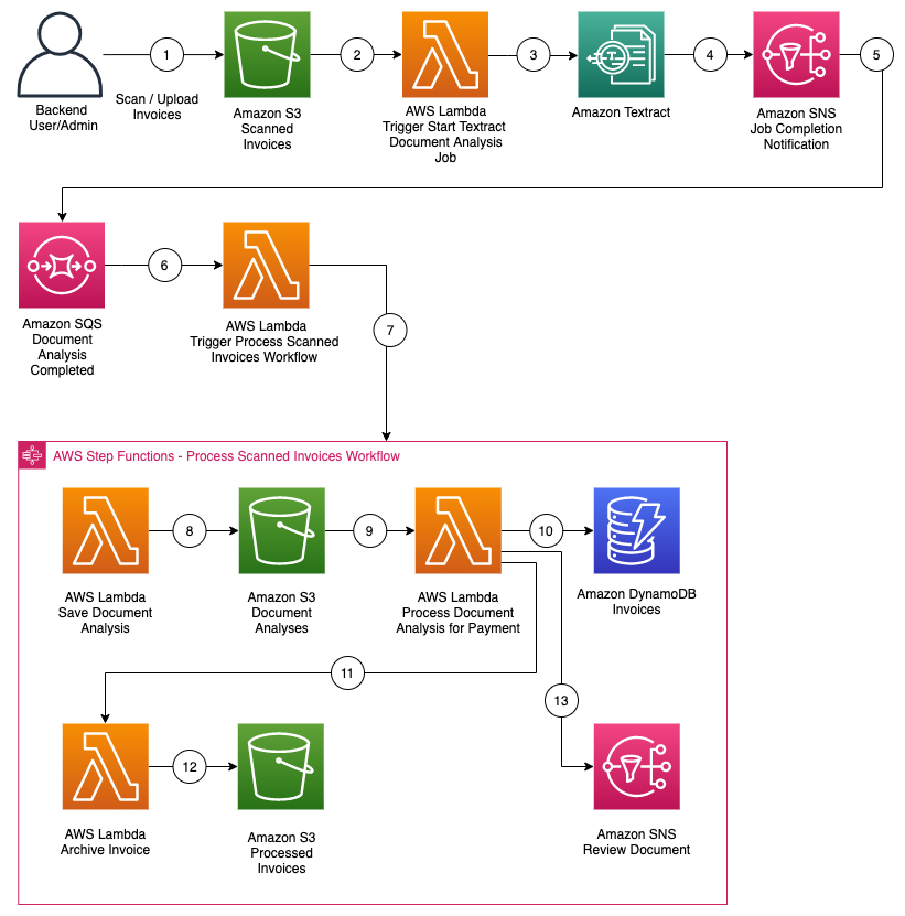
Chris Deigan is an AWS Solution Engineer in London, UK. Chris works with AWS Solution Architects to create standardized tools, code samples, demonstrations, and quick starts.


Matteo Figus is an AWS Solution Engineer based in the UK. Matteo works with the AWS Solution Architects to create standardized tools, code samples, demonstrations and quickstarts. He is passionate about open-source software and in his spare time he likes to cook and play the piano.


Nick Lee is an AWS Solution Engineer based in the UK. Nick works with the AWS Solution Architects to create standardized tools, code samples, demonstrations and quickstarts. In his spare time he enjoys playing football and squash, and binge-watching TV shows.


Adir Sharabi is a Solutions Architect with Amazon Web Services. He works with AWS customers to help them architect secure, resilient, scalable and high performance applications in the cloud. He is also passionate about Data and helping customers to get the most out of it.


Cristina Fuia is a Specialist Solutions Architect for Analytics at AWS. She works with customers across EMEA helping them to solve complex problems, design and build data architectures so that they can get business value from analyzing their data.


Choosing between AWS Lambda data storage options in web apps

Post Syndicated from James Beswick original https://aws.amazon.com/blogs/compute/choosing-between-aws-lambda-data-storage-options-in-web-apps/

AWS Lambda is an on-demand compute service that powers many serverless applications. Lambda functions are ephemeral, with execution environments only existing for a brief time when the function is invoked. Many compute operations need access to external data for a variety of purposes. This includes importing third-party libraries, accessing machine learning models, or exporting the output of the compute operation.

Lambda provides a comprehensive range of storage options to meet the needs of web application developers. These include other AWS services such as Amazon S3 and Amazon EFS. There are also native storage options available, such as temporary storage or Lambda layers. In this blog post, I explain the differences between these options, and discuss common use-cases to help you choose for your own applications.

This post references the Happy Path web application series, and you can download the code for that application from the repository.

Amazon S3 – Object storage

Amazon S3 is an object storage service that scales elastically. It offers high availability and 11 9’s of durability. The service is ideal for storing unstructured data. This includes binary data, such as images or media, log files and sensor data.

Sample contents from an S3 bucket.

There are certain characteristics of S3 object storage that are important to remember. While S3 objects can be versioned, you cannot append data as you could in a file system. You have to store an entirely new version of an object. S3 also has a flat storage hierarchy that’s different to a file system. Instead of directories, you use folders to logically organize objects, by prefixing ‘foldername/’ in the key name.

S3 has important event integrations for serverless developers. It has a native integration with Lambda, which allows you to invoke a function in response to an S3 event. This can provide a scalable way to trigger application workflows when objects are created or deleted in S3. In the Happy Path application, the image-processing workflows are initiated by this event integration. To learn more about using S3 to trigger automated serverless workflows, visit the learning path.

S3 is often an important repository for an organization’s data lake. If your application writes data to S3 buckets, this can be a useful staging area for downstream processing. For analytics workloads, you can use AWS Glue to perform extract, transform, and loan (ETL) operations. To create ad hoc visualizations and business analysis reports, Amazon QuickSight can connect to your S3 buckets and produce interactive dashboards. To learn how to build business intelligence dashboards for your web application, visit the Innovator Island workshop.

S3 also provides object lifecycle management. This allows you to automatically change storage classes when certain conditions are met. For example, an application for uploading expenses could automatically archive PDFs after 1 year to Amazon S3 Glacier to reduce storage costs. In the Happy Path application, the original high-resolution uploads are stored in a separate bucket from the optimized distribution assets. To reduce storage costs, lifecycle management could be configured to automatically delete these original photo assets after 30 days.

Temporary storage with /tmp

The Lambda execution environment provides a file system for your code to use at /tmp. This space has a fixed size of 512 MB. The same Lambda execution environment may be reused by multiple Lambda invocations to optimize performance. The /tmp area is preserved for the lifetime of the execution environment and provides a transient cache for data between invocations. Each time a new execution environment is created, this area is deleted.

Consequently, this is intended as an ephemeral storage area. While functions may cache data here between invocations, it should be used only for data needed by code in a single invocation. It’s not a place to store data permanently, and is better-used to support operations required by your code.

Operationally, working with files in /tmp is the same as your local hard disk, and offers fast I/O throughput. For example, to unzip a file into this space in Python, use:

import os, zipfile
os.chdir('/tmp')
with zipfile.ZipFile(myzipfile, 'r') as zip:
    zip.extractall()

Lambda layers

Your Lambda functions may use additional libraries as part of the deployment package. You can bundle these in the deployment archive or optionally move to a layer instead. A Lambda function can have up to five layers, and is subject to the maximum deployment size of 50 MB (zipped). Packages in layers are available in the /opt directory during invocations. While layers are private to you by default, you can also share layers with other AWS accounts, or make layers public.

Lambda layers in the console

There are many benefits to using layers throughout the functions in your serverless application. It’s best practice to include the AWS SDK instead of depending on the version bundled with the Lambda service. This enables you to pin the version of the SDK. By using a layer, you don’t need to bundle the package with each function, which can increase your deployment package size and slow down deployments. You can create an AWS SDK layer and then include a reference to the layer in each function.

Layers can be an effective way to bundle large dependencies, or share compiled libraries with binaries that vary by operating system. For example, the Happy Path application uses the Sharp npm graphics library to process images. Similarly, the Innovator Island workshop uses the OpenCV library to perform image manipulation, and this is imported using a shared layer.

Layers are static once they are deployed. You can only change the contents of a layer by deploying a new version. Any Lambda function using the layer binds to a specific version and must be updated to change layer versions. To learn more, see using Lambda layers to simplify your development process.

Amazon EFS for Lambda

Amazon EFS is a fully managed, elastic, shared file system that integrates with other AWS services. It is durable storage option that offers high availability. You can now mount EFS volumes in Lambda functions, which makes it simpler to share data across invocations. The file system grows and shrinks as you add or delete data, so you do not need to manage storage limits.

EFS file system in the console.

The Lambda service mounts EFS file systems when the execution environment is prepared. This happens in parallel with other initialization operations so typically does not impact cold start latency. If the execution environment is warm from previous invocations, the mount is already prepared. To use EFS, your Lambda function must be in the same VPC as the file system.

EFS enables new capabilities for serverless applications. The file system is a dynamic binding for Lambda functions, unlike layers. This makes it useful for deploying code libraries where you want to always use the latest version. You configure the mount path when integrating the file system with your function, and then include packages from this location. Additionally, you can use this to include packages that exceed the limits of layers.

Due to its speed and support of standard file operations, EFS is also useful for ingesting or writing large numbers files durably. This can be helpful for zipping or unzipping large archives, for example. For appending to existing files, EFS is also a preferred option to using S3.

To learn more, see using Amazon EFS for AWS Lambda in your serverless applications.

Comparing the different data storage options

This table compares the characteristics of these four different data storage options for Lambda:

Amazon S3 /tmp Lambda Layers Amazon EFS
Maximum size Elastic 512 MB 50 MB Elastic
Persistence Durable Ephemeral Durable Durable
Content Dynamic Dynamic Static Dynamic
Storage type Object File system Archive File system
Lambda event source integration Native N/A N/A N/A
Operations supported Atomic with versioning Any file system operation Immutable Any file system operation
Object tagging Y N N N
Object metadata Y N N N
Pricing model Storage + requests + data transfer Included in Lambda Included in Lambda Storage + data transfer + throughput
Sharing/permissions model IAM Function-only IAM IAM + NFS
Source for AWS Glue Y N N N
Source for Amazon QuickSight Y N N N
Relative data access speed from Lambda Fast Fastest Fastest Very fast

Conclusion

Lambda is a flexible, on-demand compute service for serverless application. It supports a wide variety of workloads by providing a number of different data storage options.

In this post, I compare the capabilities and use-cases of S3, EFS, Lambda layers, and temporary storage for Lambda functions. There are benefits to each approach, as each type has different behaviors and characteristics. For web application developers, these storage types support different operations depending upon the needs of your serverless backend.

As the newest integration with Lambda, EFS now enables new workloads and capabilities. This includes sharing large code packages with Lambda, or durably operating on large numbers of files. It also opens up new possibilities for developers working on deep learning inference models.

To learn more about storage options available, visit the AWS Serverless homepage. For more serverless learning resources, visit https://serverlessland.com.

Mercado Libre: How to Block Malicious Traffic in a Dynamic Environment

Post Syndicated from Gaston Ansaldo original https://aws.amazon.com/blogs/architecture/mercado-libre-how-to-block-malicious-traffic-in-a-dynamic-environment/

Blog post contributors: Pablo Garbossa and Federico Alliani of Mercado Libre

Introduction

Mercado Libre (MELI) is the leading e-commerce and FinTech company in Latin America. We have a presence in 18 countries across Latin America, and our mission is to democratize commerce and payments to impact the development of the region.

We manage an ecosystem of more than 8,000 custom-built applications that process an average of 2.2 million requests per second. To support the demand, we run between 50,000 to 80,000 Amazon Elastic Cloud Compute (EC2) instances, and our infrastructure scales in and out according to the time of the day, thanks to the elasticity of the AWS cloud and its auto scaling features.

Mercado Libre

As a company, we expect our developers to devote their time and energy building the apps and features that our customers demand, without having to worry about the underlying infrastructure that the apps are built upon. To achieve this separation of concerns, we built Fury, our platform as a service (PaaS) that provides an abstraction layer between our developers and the infrastructure. Each time a developer deploys a brand new application or a new version of an existing one, Fury takes care of creating all the required components such as Amazon Virtual Private Cloud (VPC), Amazon Elastic Load Balancing (ELB), Amazon EC2 Auto Scaling group (ASG), and EC2) instances. Fury also manages a per-application Git repository, CI/CD pipeline with different deployment strategies, such like blue-green and rolling upgrades, and transparent application logs and metrics collection.

Fury- MELI PaaS

For those of us on the Cloud Security team, Fury represents an opportunity to enforce critical security controls across our stack in a way that’s transparent to our developers. For instance, we can dictate what Amazon Machine Images (AMIs) are vetted for use in production (such as those that align with the Center for Internet Security benchmarks). If needed, we can apply security patches across all of our fleet from a centralized location in a very scalable fashion.

But there are also other attack vectors that every organization that has a presence on the public internet is exposed to. The AWS recent Threat Landscape Report shows a 23% YoY increase in the total number of Denial of Service (DoS) events. It’s evident that organizations need to be prepared to quickly react under these circumstances.

The variety and the number of attacks are increasing, testing the resilience of all types of organizations. This is why we started working on a solution that allows us to contain application DoS attacks, and complements our perimeter security strategy, which is based on services such as AWS Shield and AWS Web Application Firewall (WAF). In this article, we will walk you through the solution we built to automatically detect and block these events.

The strategy we implemented for our solution, Network Behavior Anomaly Detection (NBAD), consists of four stages that we repeatedly execute:

  1. Analyze the execution context of our applications, like CPU and memory usage
  2. Learn their behavior
  3. Detect anomalies, gather relevant information and process it
  4. Respond automatically

Step 1: Establish a baseline for each application

End user traffic enters through different AWS CloudFront distributions that route to multiple Elastic Load Balancers (ELBs). Behind the ELBs, we operate a fleet of NGINX servers from where we connect back to the myriad of applications that our developers create via Fury.

MELI Architecture - nomaly detection project-step 1

Step 1: MELI Architecture – Anomaly detection project

We collect logs and metrics for each application that we ship to Amazon Simple Storage Service (S3) and Datadog. We then partition these logs using AWS Glue to make them available for consumption via Amazon Athena. On average, we send 3 terabytes (TB) of log files in parquet format to S3.

Based on this information, we developed processes that we complement with commercial solutions, such as Datadog’s Anomaly Detection, which allows us to learn the normal behavior or baseline of our applications and project expected adaptive growth thresholds for each one of them.

Anomaly detection

Step 2: Anomaly detection

When any of our apps receives a number of requests that fall outside the limits set by our anomaly detection algorithms, an Amazon Simple Notification Service (SNS) event is emitted, which triggers a workflow in the Anomaly Analyzer, a custom-built component of this solution.

Upon receiving such an event, the Anomaly Analyzer starts composing the so-called event context. In parallel, the Data Extractor retrieves vital insights via Athena from the log files stored in S3.

The output of this process is used as the input for the data enrichment process. This is responsible for consulting different threat intelligence sources that are used to further augment the analysis and determine if the event is an actual incident or not.

At this point, we build the context that will allow us not only to have greater certainty in calculating the score, but it will also help us validate and act quicker. This context includes:

  • Application’s owner
  • Affected business metrics
  • Error handling statistics of our applications
  • Reputation of IP addresses and associated users
  • Use of unexpected URL parameters
  • Distribution by origin of the traffic that generated the event (cloud providers, geolocation, etc.)
  • Known behavior patterns of vulnerability discovery or exploitation
Step 2: MELI Architecture - Anomaly detection project

Step 2: MELI Architecture – Anomaly detection project

Step 3: Incident response

Once we reconstruct the context of the event, we calculate a score for each “suspicious actor” involved.

Step 3: MELI Architecture - Anomaly detection project

Step 3: MELI Architecture – Anomaly detection project

Based on these analysis results we carry out a series of verifications in order to rule out false positives. Finally, we execute different actions based on the following criteria:

Manual review

If the outcome of the automatic analysis results in a medium risk scoring, we activate a manual review process:

  1. We send a report to the application’s owners with a summary of the context. Based on their understanding of the business, they can activate the Incident Response Team (IRT) on-call and/or provide feedback that allows us to improve our automatic rules.
  2. In parallel, our threat analysis team receives and processes the event. They are equipped with tools that allow them to add IP addresses, user-agents, referrers, or regular expressions into Amazon WAF to carry out temporary blocking of “bad actors” in situations where the attack is in progress.

Automatic response

If the analysis results in a high risk score, an automatic containment process is triggered. The event is sent to our block API, which is responsible for adding a temporary rule designed to mitigate the attack in progress. Behind the scenes, our block API leverages AWS WAF to create IPSets. We reference these IPsets from our custom rule groups in our web ACLs, in order to block IPs that source the malicious traffic. We found many benefits in the new release of AWS WAF, like support for Amazon Managed Rules, larger capacity units per web ACL as well as an easier to use API.

Conclusion

By leveraging the AWS platform and its powerful APIs, and together with the AWS WAF service team and solutions architects, we were able to build an automated incident response solution that is able to identify and block malicious actors with minimal operator intervention. Since launching the solution, we have reduced YoY application downtime over 92% even when the time under attack increased over 10x. This has had a positive impact on our users and therefore, on our business.

Not only was our downtime drastically reduced, but we also cut the number of manual interventions during this type of incident by 65%.

We plan to iterate over this solution to further reduce false positives in our detection mechanisms as well as the time to respond to external threats.

About the authors

Pablo Garbossa is an Information Security Manager at Mercado Libre. His main duties include ensuring security in the software development life cycle and managing security in MELI’s cloud environment. Pablo is also an active member of the Open Web Application Security Project® (OWASP) Buenos Aires chapter, a nonprofit foundation that works to improve the security of software.

Federico Alliani is a Security Engineer on the Mercado Libre Monitoring team. Federico and his team are in charge of protecting the site against different types of attacks. He loves to dive deep into big architectures to drive performance, scale operational efficiency, and increase the speed of detection and response to security events.

Architecting a Data Lake for Higher Education Student Analytics

Post Syndicated from Craig Jordan original https://aws.amazon.com/blogs/architecture/architecting-data-lake-for-higher-education-student-analytics/

One of the keys to identifying timely and impactful actions is having enough raw material to work with. However, this up-to-date information typically lives in the databases that sit behind several different applications. One of the first steps to finding data-driven insights is gathering that information into a single store that an analyst can use without interfering with those applications.

For years, reporting environments have relied on a data warehouse stored in a single, separate relational database management system (RDBMS). But now, due to the growing use of Software as a service (SaaS) applications and NoSQL database options, data may be stored outside the data center and in formats other than tables of rows and columns. It’s increasingly difficult to access the data these applications maintain, and a data warehouse may not be flexible enough to house the gathered information.

For these reasons, reporting teams are building data lakes, and those responsible for using data analytics at universities and colleges are no different. However, it can be challenging to know exactly how to start building this expanded data repository so it can be ready to use quickly and still expandable as future requirements are uncovered. Helping higher education institutions address these challenges is the topic of this post.

About Maryville University

Maryville University is a nationally recognized private institution located in St. Louis, Missouri, and was recently named the second fastest growing private university by The Chronicle of Higher Education. Even with its enrollment growth, the university is committed to a highly personalized education for each student, which requires reliable data that is readily available to multiple departments. University leaders want to offer the right help at the right time to students who may be having difficulty completing the first semester of their course of study. To get started, the data experts in the Office of Strategic Information and members of the IT Department needed to create a data environment to identify students needing assistance.

Critical data sources

Like most universities, Maryville’s student-related data centers around two significant sources: the student information system (SIS), which houses student profiles, course completion, and financial aid information; and the learning management system (LMS) in which students review course materials, complete assignments, and engage in online discussions with faculty and fellow students.

The first of these, the SIS, stores its data in an on-premises relational database, and for several years, a significant subset of its contents had been incorporated into the university’s data warehouse. The LMS, however, contains data that the team had not tried to bring into their data warehouse. Moreover, that data is managed by a SaaS application from Instructure, called “Canvas,” and is not directly accessible for traditional extract, transform, and load (ETL) processing. The team recognized they needed a new approach and began down the path of creating a data lake in AWS to support their analysis goals.

Getting started on the data lake

The first step the team took in building their data lake made use of an open source solution that Harvard’s IT department developed. The solution, comprised of AWS Lambda functions and Amazon Simple Storage Service (S3) buckets, is deployed using AWS CloudFormation. It enables any university that uses Canvas for their LMS to implement a solution that moves LMS data into an S3 data lake on a daily basis. The following diagram illustrates this portion of Maryville’s data lake architecture:

The data lake for the Learning Management System data

Diagram 1: The data lake for the Learning Management System data

The AWS Lambda functions invoke the LMS REST API on a daily schedule resulting in Maryville’s data, which has been previously unloaded and compressed by Canvas, to be securely stored into S3 objects. AWS Glue tables are defined to provide access to these S3 objects. Amazon Simple Notification Service (SNS) informs stakeholders the status of the data loads.

Expanding the data lake

The next step was deciding how to copy the SIS data into S3. The team decided to use the AWS Database Migration Service (DMS) to create daily snapshots of more than 2,500 tables from this database. DMS uses a source endpoint for secure access to the on-premises database instance over VPN. A target endpoint determines the specific S3 bucket into which the data should be written. A migration task defines which tables to copy from the source database along with other migration options. Finally, a replication instance, a fully managed virtual machine, runs the migration task to copy the data. With this configuration in place, the data lake architecture for SIS data looks like this:

Diagram 2: Migrating data from the Student Information System

Diagram 2: Migrating data from the Student Information System

Handling sensitive data

In building a data lake you have several options for handling sensitive data including:

  • Leaving it behind in the source system and avoid copying it through the data replication process
  • Copying it into the data lake, but taking precautions to ensure that access to it is limited to authorized staff
  • Copying it into the data lake, but applying processes to eliminate, mask, or otherwise obfuscate the data before it is made accessible to analysts and data scientists

The Maryville team decided to take the first of these approaches. Building the data lake gave them a natural opportunity to assess where this data was stored in the source system and then make changes to the source database itself to limit the number of highly sensitive data fields.

Validating the data lake

With these steps completed, the team turned to the final task, which was to validate the data lake. For this process they chose to make use of Amazon Athena, AWS Glue, and Amazon Redshift. AWS Glue provided multiple capabilities including metadata extraction, ETL, and data orchestration. Metadata extraction, completed by Glue crawlers, quickly converted the information that DMS wrote to S3 into metadata defined in the Glue data catalog. This enabled the data in S3 to be accessed using standard SQL statements interactively in Athena. Without the added cost and complexity of a database, Maryville’s data analyst was able to confirm that the data loads were completing successfully. He was also able to resolve specific issues encountered on particular tables. The SQL queries, written in Athena, could later be converted to ETL jobs in AWS Glue, where they could be triggered on a schedule to create additional data in S3. Athena and Glue enabled the ETL that was needed to transform the raw data delivered to S3 into prepared datasets necessary for existing dashboards.

Once curated datasets were created and stored in S3, the data was loaded into an AWS Redshift data warehouse, which supported direct access by tools outside of AWS using ODBC/JDBC drivers. This capability enabled Maryville’s team to further validate the data by attaching the data in Redshift to existing dashboards that were running in Maryville’s own data center. Redshift’s stored procedure language allowed the team to port some key ETL logic so that the engineering of these datasets could follow a process similar to approaches used in Maryville’s on-premises data warehouse environment.

Conclusion

The overall data lake/data warehouse architecture that the Maryville team constructed currently looks like this:

The complete architecture

Diagram 3: The complete architecture

Through this approach, Maryville’s two-person team has moved key data into position for use in a variety of workloads. The data in S3 is now readily accessible for ad hoc interactive SQL workloads in Athena, ETL jobs in Glue, and ultimately for machine learning workloads running in EC2, Lambda or Amazon Sagemaker. In addition, the S3 storage layer is easy to expand without interrupting prior workloads. At the time of this writing, the Maryville team is both beginning to use this environment for machine learning models described earlier as well as adding other data sources into the S3 layer.

Acknowledgements

The solution described in this post resulted from the collaborative effort of Christine McQuie, Data Engineer, and Josh Tepen, Cloud Engineer, at Maryville University, with guidance from Travis Berkley and Craig Jordan, AWS Solutions Architects.

Optimizing the cost of serverless web applications

Post Syndicated from James Beswick original https://aws.amazon.com/blogs/compute/optimizing-the-cost-of-serverless-web-applications/

Web application backends are one of the most frequent types of serverless use-case for customers. The pay-for-value model can make it cost-efficient to build web applications using serverless tools.

While serverless cost is generally correlated with level of usage, there are architectural decisions that impact cost efficiency. The impact of these choices is more significant as your traffic grows, so it’s important to consider the cost-effectiveness of different designs and patterns.

This blog post reviews some common areas in web applications where you may be able to optimize cost. It uses the Happy Path web application as a reference example, which you can read about in the introductory blog post.

Serverless web applications generally use a combination of the services in the following diagram. I cover each of these areas to highlight common areas for cost optimization.

Serverless architecture by AWS service

The API management layer: Selecting the right API type

Most serverless web applications use an API between the frontend client and the backend architecture. Amazon API Gateway is a common choice since it is a fully managed service that scales automatically. There are three types of API offered by the service – REST APIs, WebSocket APIs, and the more recent HTTP APIs.

HTTP APIs offer many of the features in the REST APIs service, but the cost is often around 70% less. It supports Lambda service integration, JWT authorization, CORS, and custom domain names. It also has a simpler deployment model than REST APIs. This feature set tends to work well for web applications, many of which mainly use these capabilities. Additionally, HTTP APIs will gain feature parity with REST APIs over time.

The Happy Path application is designed for 100,000 monthly active users. It uses HTTP APIs, and you can inspect the backend/template.yaml to see how to define these in the AWS Serverless Application Model (AWS SAM). If you have existing AWS SAM templates that are using REST APIs, in many cases you can change these easily:

REST to HTTP API

Content distribution layer: Optimizing assets

Amazon CloudFront is a content delivery network (CDN). It enables you to distribute content globally across 216 Points of Presence without deploying or managing any infrastructure. It reduces latency for users who are geographically dispersed and can also reduce load on other parts of your service.

A typical web application uses CDNs in a couple of different ways. First, there is the distribution of the application itself. For single-page application frameworks like React or Vue.js, the build processes create static assets that are ideal for serving over a CDN.

However, these builds may not be optimized and can be larger than necessary. Many frameworks offer optimization plugins, and the JavaScript community frequently uses Webpack to bundle modules and shrink deployment packages. Similarly, any media assets used in the application build should be optimized. You can use tools like Lighthouse to analyze your web apps to find images that can be resized or compressed.

Optimizing images

The second common CDN use-case for web apps is for user-generated content (UGC). Many apps allow users to upload images, which are then shared with other users. A typical photo from a 12-megapixel smartphone is 3–9 MB in size. This high resolution is not necessary when photos are rendered within web apps. Displaying the high-resolution asset results in slower download performance and higher data transfer costs.

The Happy Path application uses a Resizer Lambda function to optimize these uploaded assets. This process creates two different optimized images depending upon which component loads the asset.

Image sizes in front-end applications

The upload S3 bucket shows the original size of the upload from the smartphone:

The distribution S3 bucket contains the two optimized images at different sizes:

Optimized images in the distribution S3 bucket

The distribution file sizes are 98–99% smaller. For a busy web application, using optimized image assets can make a significant difference to data transfer and CloudFront costs.

Additionally, you can convert to highly optimized file formats such as WebP to reduce file size even further. Not all browsers support this format, but you can use CSS on the frontend to fall back to other types if needed:

<img src="myImage.webp" onerror="this.onerror=null; this.src='myImage.jpg'">

The data layer

AWS offers many different database and storage options that can be useful for web applications. Billing models vary by service and Region. By understanding the data access and storage requirements of your app, you can make informed decisions about the right service to use.

Generally, it’s more cost-effective to store binary data in S3 than a database. First, when the data is uploaded, you can upload directly to S3 with presigned URLs instead of proxying data via API Gateway or another service.

If you are using Amazon DynamoDB, it’s best practice to store larger items in S3 and include a reference token in a table item. Part of DynamoDB pricing is based on read capacity units (RCUs). For binary items such as images, it is usually more cost-efficient to use S3 for storage.

Many web developers who are new to serverless are familiar with using a relational database, so choose Amazon RDS for their database needs. Depending upon your use-case and data access patterns, it may be more cost effective to use DynamoDB instead. RDS is not a serverless service so there are monthly charges for the underlying compute instance. DynamoDB pricing is based upon usage and storage, so for many web apps may be a lower-cost choice.

Integration layer

This layer includes services like Amazon SQS, Amazon SNS, and Amazon EventBridge, which are essential for decoupling serverless applications. Each of these have a request-based pricing component, where 64 KB of a payload is billed as one request. For example, a single SQS message with a 256 KB payload is billed as four requests. There are two optimization methods common for web applications.

1. Combine messages

Many messages sent to these services are much smaller than 64 KB. In some applications, the publishing service can combine multiple messages to reduce the total number of publish actions to SNS. Additionally, by either eliminating unused attributes in the message or compressing the message, you can store more data in a single request.

For example, a publishing service may be able to combine multiple messages together in a single publish action to an SNS topic:

  • Before optimization, a publishing service sends 100,000,000 1KB-messages to an SNS topic. This is charged as 100 million messages for a total cost of $50.00.
  • After optimization, the publishing service combines messages to send 1,562,500 64KB-messages to an SNS topic. This is charged as 1,562,500 messages for a total cost of $0.78.

2. Filter messages

In many applications, not every message is useful for a consuming service. For example, an SNS topic may publish to a Lambda function, which checks the content and discards the message based on some criteria. In this case, it’s more cost effective to use the native filtering capabilities of SNS. The service can filter messages and only invoke the Lambda function if the criteria is met. This lowers the compute cost by only invoking Lambda when necessary.

For example, an SNS topic receives messages about customer orders and forwards these to a Lambda function subscriber. The function is only interested in canceled orders and discards all other messages:

  • Before optimization, the SNS topic sends all messages to a Lambda function. It evaluates the message for the presence of an order canceled attribute. On average, only 25% of the messages are processed further. While SNS does not charge for delivery to Lambda functions, you are charged each time the Lambda service is invoked, for 100% of the messages.
  • After optimization, using an SNS subscription filter policy, the SNS subscription filters for canceled orders and only forwards matching messages. Since the Lambda function is only invoked for 25% of the messages, this may reduce the total compute cost by up to 75%.

3. Choose a different messaging service

For complex filtering options based upon matching patterns, you can use EventBridge. The service can filter messages based upon prefix matching, numeric matching, and other patterns, combining several rules into a single filter. You can create branching logic within the EventBridge rule to invoke downstream targets.

EventBridge offers a broader range of targets than SNS destinations. In cases where you publish from an SNS topic to a Lambda function to invoke an EventBridge target, you could use EventBridge instead and eliminate the Lambda invocation. For example, instead of routing from SNS to Lambda to AWS Step Functions, instead create an EventBridge rule that routes events directly to a state machine.

Business logic layer

Step Functions allows you to orchestrate complex workflows in serverless applications while eliminating common boilerplate code. The Standard Workflow service charges per state transition. Express Workflows were introduced in December 2019, with pricing based on requests and duration, instead of transitions.

For workloads that are processing large numbers of events in shorter durations, Express Workflows can be more cost-effective. This is designed for high-volume event workloads, such as streaming data processing or IoT data ingestion. For these cases, compare the cost of the two workflow types to see if you can reduce cost by switching across.

Lambda is the on-demand compute layer in serverless applications, which is billed by requests and GB-seconds. GB-seconds is calculated by multiplying duration in seconds by memory allocated to the function. For a function with a 1-second duration, invoked 1 million times, here is how memory allocation affects the total cost in the US East (N. Virginia) Region:

Memory (MB) GB/S Compute cost Total cost
128 125,000 $ 2.08 $ 2.28
512 500,000 $ 8.34 $ 8.54
1024 1,000,000 $ 16.67 $ 16.87
1536 1,500,000 $ 25.01 $ 25.21
2048 2,000,000 $ 33.34 $ 33.54
3008 2,937,500 $ 48.97 $ 49.17

There are many ways to optimize Lambda functions, but one of the most important choices is memory allocation. You can choose between 128 MB and 3008 MB, but this also impacts the amount of virtual CPU as memory increases. Since total cost is a combination of memory and duration, choosing more memory can often reduce duration and lower overall cost.

Instead of manually setting the memory for a Lambda function and running executions to compare duration, you can use the AWS Lambda Power Tuning tool. This uses Step Functions to run your function against varying memory configurations. It can produce a visualization to find the optimal memory setting, based upon cost or execution time.

Optimizing costs with the AWS Lambda Power Tuning tool

Conclusion

Web application backends are one of the most popular workload types for serverless applications. The pay-per-value model works well for this type of workload. As traffic grows, it’s important to consider the design choices and service configurations used to optimize your cost.

Serverless web applications generally use a common range of services, which you can logically split into different layers. This post examines each layer and suggests common cost optimizations helpful for web app developers.

To learn more about building web apps with serverless, see the Happy Path series. For more serverless learning resources, visit https://serverlessland.com.

Apply record level changes from relational databases to Amazon S3 data lake using Apache Hudi on Amazon EMR and AWS Database Migration Service

Post Syndicated from Ninad Phatak original https://aws.amazon.com/blogs/big-data/apply-record-level-changes-from-relational-databases-to-amazon-s3-data-lake-using-apache-hudi-on-amazon-emr-and-aws-database-migration-service/

Data lakes give organizations the ability to harness data from multiple sources in less time. Users across different roles are now empowered to collaborate and analyze data in different ways, leading to better, faster decision-making. Amazon Simple Storage Service (Amazon S3) is the highly performant object storage service for structured and unstructured data and the storage service of choice to build a data lake.

However, many use cases like performing change data capture (CDC) from an upstream relational database to an Amazon S3-based data lake require handling data at a record level. Performing an operation like inserting, updating, and deleting individual records from a dataset requires the processing engine to read all the objects (files), make the changes, and rewrite the entire dataset as new files. Furthermore, making the data available in the data lake in near-real time often leads to the data being fragmented over many small files, resulting in poor query performance. Apache Hudi is an open-source data management framework that enables you to manage data at the record level in Amazon S3 data lakes, thereby simplifying building CDC pipelines and making it efficient to do streaming data ingestion. Datasets managed by Hudi are stored in Amazon S3 using open storage formats, and integrations with Presto, Apache Hive, Apache Spark, and the AWS Glue Data Catalog give you near real-time access to updated data using familiar tools. Hudi is supported in Amazon EMR and is automatically installed when you choose Spark, Hive, or Presto when deploying your EMR cluster.

In this post, we show you how to build a CDC pipeline that captures the data from an Amazon Relational Database Service (Amazon RDS) for MySQL database using AWS Database Migration Service (AWS DMS) and applies those changes to a dataset in Amazon S3 using Apache Hudi on Amazon EMR. Apache Hudi includes the utility HoodieDeltaStreamer, which provides an easy way to ingest data from many sources, such as a distributed file system or Kafka. It manages checkpointing, rollback, and recovery so you don’t need to keep track of what data has been read and processed from the source, which makes it easy to consume change data. It also allows for lightweight SQL-based transformations on the data as it is being ingested. For more information, see Writing Hudi Tables. Support for AWS DMS with HoodieDeltaStreamer is provided with Apache Hudi version 0.5.2 and is available on Amazon EMR 5.30.x and 6.1.0.

Architecture overview

The following diagram illustrates the architecture we deploy to build our CDC pipeline.

In this architecture, we have a MySQL instance on Amazon RDS. AWS DMS pulls full and incremental data (using the CDC feature of AWS DMS) into an S3 bucket in Parquet format. HoodieDeltaStreamer on an EMR cluster is used to process the full and incremental data to create a Hudi dataset. As the data in the MySQL database gets updated, the AWS DMS task picks up the changes and takes them to the raw S3 bucket. The HoodieDeltastreamer job can be run on the EMR cluster at a certain frequency or in a continuous mode to apply these changes to the Hudi dataset in the Amazon S3 data lake. You can query this data with tools such as SparkSQL, Presto, Apache Hive running on the EMR cluster, and Amazon Athena.

Deploying the solution resources

We use AWS CloudFormation to deploy these components in your AWS account. Choose an AWS Region for deployment where the following services are available:

You need to meet the following prerequisites before deploying the CloudFormation template:

  • Have a VPC with at least two public subnets in your account.
  • Have a S3 bucket where you want to collect logs from the EMR cluster. This should be in the same AWS region where you spin up the CloudFormation stack.
  • Have an AWS Identity and Access Management (IAM) role dms-vpc-role. For instructions on creating one, see Security in AWS Database Migration Service.
  • If you’re deploying the stack in an account using the AWS Lake Formation permission model, validate the following settings:
    • The IAM user used to deploy the stack is added as a data lake administrator under Lake Formation or the IAM user used to deploy the stack has IAM privileges to create databases in the AWS Glue Data Catalog.
    • The Data Catalog settings under Lake Formation are configured to use only IAM access control for new databases and new tables in new databases. This makes sure that all access to the newly created databases and tables in the Data Catalog are controlled solely using IAM permissions.
  • IAMAllowedPrincipals is granted database creator privilege on the Lake Formation Database creators page.

If this privilege is not in place, grant it by choosing Grant and selecting the Create database permission.

These Lake Formation settings are required so that all permissions to the Data Catalog objects are controlled using IAM only.

Launching the CloudFormation stack

To launch the CloudFormation stack, complete the following steps:

  1. Choose Launch Stack:
  2. Provide the mandatory parameters in the Parameters section, including an S3 bucket to store the Amazon EMR logs and a CIDR IP range from where you want to access Amazon RDS for MySQL.
  3. Follow through the CloudFormation stack creation wizard, leaving rest of the default values unchanged.
  4. On the final page, select I acknowledge that AWS CloudFormation might create IAM resources with custom names.
  5. Choose Create stack.
  6. When the stack creation is complete, record the details of the S3 bucket, EMR cluster, and Amazon RDS for MySQL details on the Outputs tab of the CloudFormation stack.

The CloudFormation template uses m5.xlarge and m5.2xlarge instances for the EMR cluster. If these instance types aren’t available in the Region or Availability Zone you have selected for deployment, the creation of the CloudFormation stack fails. If that happens, choose a Region or subnet where the instance type is available. For more information about working around this issue, see Instance Type Not Supported.

CloudFormation also creates and configures the AWS DMS endpoints and tasks with requisite connection attributes such as dataFormat, timestampColumnName, and parquetTimestampInMillisecond. For more information, see Extra connection attributes when using Amazon S3 as a target for AWS DMS.

The database instance deployed as part of the CloudFormation stack has already been created with the settings needed for AWS DMS to work in CDC mode on the database. These are:

  • binlog_format=ROW
  • binlog_checksum=NONE

Also, automatic backups are enabled on the RDS DB instance. This is a required attribute for AWS DMS to do CDC. For more information, see Using a MySQL-compatible database as a source for AWS DMS.

Running the end-to-end data flow

Now that the CloudFormation stack is deployed, we can run our data flow to get the full and incremental data from MySQL into a Hudi dataset in our data lake.

  1. As a best practice, retain your binlogs for at least 24 hours. Log in to your Amazon RDS for MySQL database using your SQL client and run the following command:
    call mysql.rds_set_configuration('binlog retention hours', 24)

  2. Create a table in the dev database:
    create table dev.retail_transactions(
    tran_id INT,
    tran_date DATE,
    store_id INT,
    store_city varchar(50),
    store_state char(2),
    item_code varchar(50),
    quantity INT,
    total FLOAT);

  3. When the table is created, insert some dummy data into the database:
    insert into dev.retail_transactions values(1,'2019-03-17',1,'CHICAGO','IL','XXXXXX',5,106.25);
    insert into dev.retail_transactions values(2,'2019-03-16',2,'NEW YORK','NY','XXXXXX',6,116.25);
    insert into dev.retail_transactions values(3,'2019-03-15',3,'SPRINGFIELD','IL','XXXXXX',7,126.25);
    insert into dev.retail_transactions values(4,'2019-03-17',4,'SAN FRANCISCO','CA','XXXXXX',8,136.25);
    insert into dev.retail_transactions values(5,'2019-03-11',1,'CHICAGO','IL','XXXXXX',9,146.25);
    insert into dev.retail_transactions values(6,'2019-03-18',1,'CHICAGO','IL','XXXXXX',10,156.25);
    insert into dev.retail_transactions values(7,'2019-03-14',2,'NEW YORK','NY','XXXXXX',11,166.25);
    insert into dev.retail_transactions values(8,'2019-03-11',1,'CHICAGO','IL','XXXXXX',12,176.25);
    insert into dev.retail_transactions values(9,'2019-03-10',4,'SAN FRANCISCO','CA','XXXXXX',13,186.25);
    insert into dev.retail_transactions values(10,'2019-03-13',1,'CHICAGO','IL','XXXXXX',14,196.25);
    insert into dev.retail_transactions values(11,'2019-03-14',5,'CHICAGO','IL','XXXXXX',15,106.25);
    insert into dev.retail_transactions values(12,'2019-03-15',6,'CHICAGO','IL','XXXXXX',16,116.25);
    insert into dev.retail_transactions values(13,'2019-03-16',7,'CHICAGO','IL','XXXXXX',17,126.25);
    insert into dev.retail_transactions values(14,'2019-03-16',7,'CHICAGO','IL','XXXXXX',17,126.25);
    

    We now use AWS DMS to start pushing this data to Amazon S3.

  4. On the AWS DMS console, run the task hudiblogload.

This task does a full load of the table to Amazon S3 and then starts writing incremental data.

If you’re prompted to test the AWS DMS endpoints while starting the AWS DMS task for the first time, you should do so. It’s generally a good practice to test the source and target endpoints before starting an AWS DMS task for the first time.

In a few minutes, the status of the task changes to Load complete, replication ongoing, which means that the full load is complete and the ongoing replication has started. You can go to the S3 bucket created by the stack and you should see a .parquet file under the dmsdata/dev/retail_transactions folder in your S3 bucket.

  1. On the Hardware tab of your EMR cluster, choose the master instance group and note the EC2 instance ID for the master instance.
  2. On the Systems Manager console, choose Session Manager.
  3. Choose Start Session to start a session with the master node of your cluster.

If you face challenges connecting to the master instance of the EMR cluster, see Troubleshooting Session Manager.

  1. Switch the user to Hadoop by running the following command:
    sudo su hadoop

In a real-life use case, the AWS DMS task starts writing incremental files to the same Amazon S3 location when the full load is complete. The way to distinguish full load vs. incremental load files is that the full load files have a name starting with LOAD, whereas CDC filenames have datetimestamps, as you see in a later step. From a processing perspective, we want to process the full load into the Hudi dataset and then start incremental data processing. To do this, we move the full load files to a different S3 folder under the same S3 bucket and process those before we start processing incremental files.

  1. Run the following command on the master node of the EMR cluster (replace <s3-bucket-name> with your actual bucket name):
    aws s3 mv s3://<s3-bucket-name>/dmsdata/dev/retail_transactions/ s3://<s3-bucket-name>/dmsdata/data-full/dev/retail_transactions/  --exclude "*" --include "LOAD*.parquet" --recursive

With the full table dump available in the data-full folder, we now use the HoodieDeltaStreamer utility on the EMR cluster to populate the Hudi dataset on Amazon S3.

  1. Run the following command to populate the Hudi dataset to the hudi folder in the same S3 bucket (replace <s3-bucket-name> with the name of the S3 bucket created by the CloudFormation stack):
    spark-submit --class org.apache.hudi.utilities.deltastreamer.HoodieDeltaStreamer  \
      --packages org.apache.hudi:hudi-utilities-bundle_2.11:0.5.2-incubating,org.apache.spark:spark-avro_2.11:2.4.5 \
      --master yarn --deploy-mode cluster \
    --conf spark.serializer=org.apache.spark.serializer.KryoSerializer \
    --conf spark.sql.hive.convertMetastoreParquet=false \
    /usr/lib/hudi/hudi-utilities-bundle_2.11-0.5.2-incubating.jar \
      --table-type COPY_ON_WRITE \
      --source-ordering-field dms_received_ts \
      --props s3://<s3-bucket-name>/properties/dfs-source-retail-transactions-full.properties \
      --source-class org.apache.hudi.utilities.sources.ParquetDFSSource \
      --target-base-path s3://<s3-bucket-name>/hudi/retail_transactions --target-table hudiblogdb.retail_transactions \
      --transformer-class org.apache.hudi.utilities.transform.SqlQueryBasedTransformer \
        --payload-class org.apache.hudi.payload.AWSDmsAvroPayload \
    --schemaprovider-class org.apache.hudi.utilities.schema.FilebasedSchemaProvider \
      --enable-hive-sync
    

The preceding command runs a Spark job that runs the HoodieDeltaStreamer utility. For more information about the parameters used in this command, see Writing Hudi Tables.

When the Spark job is complete, you can navigate to the AWS Glue console and find a table called retail_transactions created under the hudiblogdb database. The input format for the table is org.apache.hudi.hadoop.HoodieParquetInputFormat.

Next, we query the data and look at the data in the retail_transactions table in the catalog.

  1. In the Systems Manager session established earlier, run the following command (make sure that you have completed all the prerequisites for the post, including adding IAMAllowedPrincipals as a database creator in Lake Formation):
    spark-shell --conf "spark.serializer=org.apache.spark.serializer.KryoSerializer" --conf "spark.sql.hive.convertMetastoreParquet=false" \
    --packages org.apache.hudi:hudi-spark-bundle_2.11:0.5.2-incubating,org.apache.spark:spark-avro_2.11:2.4.5 \
    --jars /usr/lib/hudi/hudi-spark-bundle_2.11-0.5.2-incubating.jar,/usr/lib/spark/external/lib/spark-avro.jar
    

  2. Run the following query on the retail_transactions table:
    spark.sql("Select * from hudiblogdb.retail_transactions order by tran_id").show()

You should see the same data in the table as the MySQL database with a few columns added by the HoodieDeltaStreamer process.

We now run some DML statements on our MySQL database and take these changes through to the Hudi dataset.

  1. Run the following DML statements on the MySQL database:
    insert into dev.retail_transactions values(15,'2019-03-16',7,'CHICAGO','IL','XXXXXX',17,126.25);
    update dev.retail_transactions set store_city='SPRINGFIELD' where tran_id=12;
    delete from dev.retail_transactions where tran_id=2;

In a few minutes, you see a new .parquet file created under dmsdata/dev/retail_transactions folder in the S3 bucket.

  1. Run the following command on the EMR cluster to get the incremental data to the Hudi dataset (replace <s3-bucket-name> with the name of the S3 bucket created by the CloudFormation template):
    spark-submit --class org.apache.hudi.utilities.deltastreamer.HoodieDeltaStreamer  \
      --packages org.apache.hudi:hudi-utilities-bundle_2.11:0.5.2-incubating,org.apache.spark:spark-avro_2.11:2.4.5 \
      --master yarn --deploy-mode cluster \
    --conf spark.serializer=org.apache.spark.serializer.KryoSerializer \
    --conf spark.sql.hive.convertMetastoreParquet=false \
    /usr/lib/hudi/hudi-utilities-bundle_2.11-0.5.2-incubating.jar \
      --table-type COPY_ON_WRITE \
      --source-ordering-field dms_received_ts \
      --props s3://<s3-bucket-name>/properties/dfs-source-retail-transactions-incremental.properties \
      --source-class org.apache.hudi.utilities.sources.ParquetDFSSource \
      --target-base-path s3://<s3-bucket-name>/hudi/retail_transactions --target-table hudiblogdb.retail_transactions \
      --transformer-class org.apache.hudi.utilities.transform.SqlQueryBasedTransformer \
        --payload-class org.apache.hudi.payload.AWSDmsAvroPayload \
    --schemaprovider-class org.apache.hudi.utilities.schema.FilebasedSchemaProvider \
      --enable-hive-sync \
    --checkpoint 0

The key difference between this command and the previous one is in the properties file that was used as an argument to the –-props and --checkpoint parameters. For the earlier command that performed the full load, we used dfs-source-retail-transactions-full.properties; for the incremental one, we used dfs-source-retail-transactions-incremental.properties. The differences between these two property files are:

  • The location of source data changes between full and incremental data in Amazon S3.
  • The SQL transformer query included a hard-coded Op field for the full load task, because an AWS DMS first-time full load doesn’t include the Op field for Parquet datasets. The Op field can have values of I, U, and D—for Insert, Update and Delete indicators.

We cover the details of the --checkpoint parameter in the Considerations when deploying to production section later in this post.

  1. When the job is complete, run the same query in spark-shell.

You should see these updates applied to the Hudi dataset.

You can use the Hudi CLI to administer Hudi datasets to view information about commits, the filesystem, statistics, and more.

  1. To do this, in the Systems Manager session, run the following command:
    /usr/lib/hudi/cli/bin/hudi-cli.sh

  2. Inside the Hudi-cli, run the following command (replace the <s3-bucket-name> with the S3 bucket created by the Cloud Formation stack):
    connect --path s3://<s3-bucket-name>/hudi/retail_transactions

  3. To inspect commits on your Hudi dataset, run the following command:
    commits show

You can also query incremental data from the Hudi dataset. This is particularly useful when you want to take incremental data for downstream processing like aggregations. Hudi provides multiple ways of pulling data incrementally which is documented here. An example of how to use this feature is available in the Hudi Quick Start Guide.

Considerations when deploying to production

The preceding setup showed an example of how to build a CDC pipeline from your relational database to your Amazon S3-based data lake. However, if you want to use this solution for production, you should consider the following:

  • To ensure high availability, you can set up the AWS DMS instance in a Multi-AZ configuration.
  • The CloudFormation stack deployed the required properties files needed by the deltastreamer utility into the S3 bucket at s3://<s3-bucket-name>/properties/. You may need to customize these based on your requirements. For more information, see Configurations. There are a few parameters that may need your attention:
    • deltastreamer.transformer.sql – This property exposes an extremely powerful feature of the deltastreamer utility: it enables you to transform data on the fly as it’s being ingested and persisted in the Hudi dataset. In this post, we have shown a basic transformation that casts the tran_date column to a string, but you can apply any transformation as part of this query.
    • parquet.small.file.limit – This field is in bytes and a critical storage configuration specifying how Hudi handles small files on Amazon S3. Small files can happen due to the number of records being processed in each insert per partition. Setting this value allows Hudi to continue to treat inserts in a particular partition as updates to the existing files, causing files that are up to the size of this small.file.limit to be rewritten and keep growing in size.
    • parquet.max.file.size – This is the max file size of a single Parquet in your Hudi dataset, after which a new file is created to store more data. For Amazon S3 storage and data querying needs, we can keep this around 256 MB–1 GB (256x1024x1024 = 268435456).
    • [Insert|Upsert|bulkinsert].shuffle.parallelism – In this post, we dealt with a small dataset of few records only. However, in real-life situations, you might want to bring in hundreds of millions of records in the first load, and then incremental CDC can potentially be in millions per day. There is a very important parameter to set when you want quite predictable control on the number of files in each of your Hudi dataset partitions. This is also needed to ensure you don’t hit an Apache Spark limit of 2 GB for data shuffle blocks when processing large amounts of data. For example, if you plan to load 200 GBs of data in first load and want to keep file sizes of approximately 256 MB, set the shuffle parallelism parameters for this dataset as 800 (200×1024/256). For more information, see Tuning Guide.
  • In the incremental load deltastreamer command, we used an additional parameter: --checkpoint 0. When deltastreamer writes a Hudi dataset, it persists checkpoint information in the .commit files under the .hoodie folder. It uses this information in subsequent runs and only reads that data from Amazon S3, which is created after this checkpoint time. In a production scenario, after you start the AWS DMS task, the task keeps writing incremental data to the target S3 folder as soon as the full load is complete. In the steps that we followed, we ran a command on the EMR cluster to manually move the full load files to another folder and process the data from there. When we did that, the timestamp associated with the S3 objects changes to the most current timestamp. If we run the incremental load without the checkpoint argument, deltastreamer doesn’t pick up any incremental data written to Amazon S3 before we manually moved the full load files. To make sure that all incremental data is processed by deltastreamer the first time, set the checkpoint to 0, which makes it process all incremental data in the folder. However, only use this parameter for the first incremental load and let deltastreamer use its own checkpointing methodology from that point onwards.
  • For this post, we ran the spark-submit command manually. However, in production, you can run it as a step on the EMR cluster.
  • You can either schedule the incremental data load command to run at a regular interval using a scheduling or orchestration tool, or run it in a continuous fashion at a certain frequency by passing additional parameters to the spark-submit command --min-sync-interval-seconds XX –continuous, where XX is the number of seconds between each run of the data pull. For example, if you want to run the processing every 5 minutes, replace XX with 300.

Cleaning up

When you are done exploring the solution, complete the following steps to clean up the resources deployed by CloudFormation:

  1. Empty the S3 bucket created by the CloudFormation stack
  2. Delete any Amazon EMR log files generated under s3://<EMR-Logs-S3-Bucket> /HudiBlogEMRLogs/.
  3. Stop the AWS DMS task Hudiblogload.
  4. Delete the CloudFormation stack.
  5. Delete any Amazon RDS for MySQL database snapshots retained after the CloudFormation template is deleted.

Conclusion

More and more data lakes are being built on Amazon S3, and these data lakes often need to be hydrated with change data from transactional systems. Handling deletes and upserts of data into the data lake using traditional methods involves a lot of heavy lifting. In this post, we saw how to easily build a solution with AWS DMS and HoodieDeltaStreamer on Amazon EMR. We also looked at how to perform lightweight record-level transformations when integrating data into the data lake, and how to use this data for downstream processes like aggregations. We also discussed the important settings and command line options that were used and how you could modify them to suit your requirements.


About the Authors

Ninad Phatak is a Senior Analytics Specialist Solutions Architect with Amazon Internet Services Private Limited. He specializes in data engineering and datawarehousing technologies and helps customers architect their analytics use cases and platforms on AWS.


Raghu Dubey is a Senior Analytics Specialist Solutions Architect with Amazon Internet Services Private Limited. He specializes in Big Data Analytics, Data warehousing and BI and helps customers build scalable data analytics platforms.