Tag Archives: Architecture

Let’s Architect! Designing event-driven architectures

Post Syndicated from Luca Mezzalira original https://aws.amazon.com/blogs/architecture/lets-architect-designing-event-driven-architectures/

During the design of distributed systems, we have to identify a communication strategy to exchange information between different services while keeping the evolutionary nature of the architecture in mind. Event-driven architectures are based on events (facts that happened in a system), which are asynchronously exchanged to implement communication across different services while having a high degree of decoupling. This paradigm also allows us to run code in response to events, with benefits like cost optimization and sustainability for the entire infrastructure.

In this edition of Let’s Architect!, we share architectural resources to introduce event-driven architectures, how to build them on AWS, and how to approach the design phase.

AWS re:Invent 2022 – Keynote with Dr. Werner Vogels

re:Invent 2022 may be finished, but the keynote given by Amazon’s Chief Technology Officer, Dr. Werner Vogels, will not be forgotten. Vogels not only covered the announcements of new services but also event-driven architecture foundations in conjunction with customers’ stories on how this architecture helped to improve their systems.

Take me to this re:Invent 2022 video!

Dr. Werner Vogels presenting an example of architecture where Amazon EventBridge is used as event bus

Dr. Werner Vogels presenting an example of architecture where Amazon EventBridge is used as event bus

Benefits of migrating to event-driven architecture

In this blog post, we enumerate clearly and concisely the benefits of event-driven architectures, such as scalability, fault tolerance, and developer velocity. This is a great post to start your journey into the event-driven architecture style, as it explains the difference from request-response architecture.

Take me to this Compute Blog post!

Two common options when building applications are request-response and event-driven architecture

Two common options when building applications are request-response and event-driven architectures

Building next-gen applications with event-driven architectures

When we build distributed systems or migrate from a monolithic to a microservices architecture, we need to identify a communication strategy to integrate the different services. Teams who are building microservices often find that integration with other applications and external services can make their workloads tightly coupled.

In this re:Invent 2022 video, you learn how to use event-driven architectures to decouple and decentralize application components through asynchronous communication. The video introduces the differences between synchronous and asynchronous communications before drilling down into some key concepts for designing and building event-driven architectures on AWS.

Take me to this re:Invent 2022 video!

How to use choreography to exchange information across services plus implement orchestration for managing operations within the service boundaries

How to use choreography to exchange information across services plus implement orchestration for managing operations within the service boundaries

Designing events

When starting on the journey to event-driven architectures, a common challenge is how to design events: “how much data should an event contain?” is a typical first question we encounter.

In this pragmatic post, you can explore the different types of events, watch a video that explains even further how to use event-driven architectures, and also go through the new event-driven architecture section of serverlessland.com.

Take me to Serverless Land!

An example of events with sparse and full state description

An example of events with sparse and full state description

See you next time!

Thanks for reading our first blog of 2023! Join us next time, when we’ll talk about architecture and sustainability.

To find all the blogs from this series, visit the Let’s Architect! section of the AWS Architecture Blog.

Text analytics on AWS: implementing a data lake architecture with OpenSearch

Post Syndicated from Francisco Losada original https://aws.amazon.com/blogs/architecture/text-analytics-on-aws-implementing-a-data-lake-architecture-with-opensearch/

Text data is a common type of unstructured data found in analytics. It is often stored without a predefined format and can be hard to obtain and process.

For example, web pages contain text data that data analysts collect through web scraping and pre-process using lowercasing, stemming, and lemmatization. After pre-processing, the cleaned text is analyzed by data scientists and analysts to extract relevant insights.

This blog post covers how to effectively handle text data using a data lake architecture on Amazon Web Services (AWS). We explain how data teams can independently extract insights from text documents using OpenSearch as the central search and analytics service. We also discuss how to index and update text data in OpenSearch and evolve the architecture towards automation.

Architecture overview

This architecture outlines the use of AWS services to create an end-to-end text analytics solution, starting from the data collection and ingestion up to the data consumption in OpenSearch (Figure 1).

Data lake architecture with OpenSearch

Figure 1. Data lake architecture with OpenSearch

  1. Collect data from various sources, such as SaaS applications, edge devices, logs, streaming media, and social networks.
  2. Use tools like AWS Database Migration Service (AWS DMS), AWS DataSync, Amazon Kinesis, Amazon Managed Streaming for Apache Kafka (Amazon MSK), AWS IoT Core, and Amazon AppFlow to ingest the data into the AWS data lake, depending on the data source type.
  3. Store the ingested data in the raw zone of the Amazon Simple Storage Service (Amazon S3) data lake—a temporary area where data is kept in its original form.
  4. Validate, clean, normalize, transform, and enrich the data through a series of pre-processing steps using AWS Glue or Amazon EMR.
  5. Place the data that is ready to be indexed in the indexing zone.
  6. Use AWS Lambda to index the documents into OpenSearch and store them back in the data lake with a unique identifier.
  7. Use the clean zone as the source of truth for teams to consume the data and calculate additional metrics.
  8. Develop, train, and generate new metrics using machine learning (ML) models with Amazon SageMaker or artificial intelligence (AI) services like Amazon Comprehend.
  9. Store the new metrics in the enriching zone along with the identifier of the OpenSearch document.
  10. Use the identifier column from the initial indexing phase to identify the correct documents and update them in OpenSearch with the newly calculated metrics using AWS Lambda.
  11. Use OpenSearch to search through the documents and visualize them with metrics using OpenSearch Dashboards.

Considerations

Data lake orchestration among teams

This architecture allows data teams to work independently on text documents at different stages of their lifecycles. The data engineering team manages the raw and indexing zones, who also handle data ingestion and preprocessing for indexing in OpenSearch.

The cleaned data is stored in the clean zone, where data analysts and data scientists generate insights and calculate new metrics. These metrics are stored in the enrich zone and indexed as new fields in the OpenSearch documents by the data engineering team (Figure 2).

Data lake orchestration among teams

Figure 2. Data lake orchestration among teams

Let’s explore an example. Consider a company that periodically retrieves blog site comments and performs sentiment analysis using Amazon Comprehend. In this case:

  1. The comments are ingested into the raw zone of the data lake.
  2. The data engineering team processes the comments and stores them in the indexing zone.
  3. A Lambda function indexes the comments into OpenSearch, enriches the comments with the OpenSearch document ID, and saves it in the clean zone.
  4. The data science team consumes the comments and performs sentiment analysis using Amazon Comprehend.
  5. The sentiment analysis metrics are stored in the metrics zone of the data lake. A second Lambda function updates the comments in OpenSearch with the new metrics.

If the raw data does not require any preprocessing steps, the indexing and clean zones can be combined. You can explore this specific example, along with code implementation, in the AWS samples repository.

Schema evolution

As your data progresses through data lake stages, the schema changes and gets enriched accordingly. Continuing with our previous example, Figure 3 explains how the schema evolves.

Schema evolution through the data lake stages

Figure 3. Schema evolution through the data lake stages

  1. In the raw zone, there is a raw text field received directly from the ingestion phase. It’s best practice to keep a raw version of the data as a backup, or in case the processing steps need to be repeated later.
  2. In the indexing zone, the clean text field replaces the raw text field after being processed.
  3. In the clean zone, we add a new ID field that is generated during indexing and identifies the OpenSearch document of the text field.
  4. In the enrich zone, the ID field is required. Other fields with metric names are optional and represent new metrics calculated by other teams that will be added to OpenSearch.

Consumption layer with OpenSearch

In OpenSearch, data is organized into indices, which can be thought of as tables in a relational database. Each index consists of documents—similar to table rows—and multiple fields, similar to table columns. You can add documents to an index by indexing and updating them using various client APIs for popular programming languages.

Now, let’s explore how our architecture integrates with OpenSearch in the indexing and updating stage.

Indexing and updating documents using Python

The index document API operation allows you to index a document with a custom ID, or assigns one if none is provided. To speed up indexing, we can use the bulk index API to index multiple documents in one call.

We need to store the IDs back from the index operation to later identify the documents we’ll update with new metrics. Let’s explore two ways of doing this:

  • Use the requests library to call the REST Bulk Index API (preferred): the response returns the auto-generated IDs we need.
  • Use the Python Low-Level Client for OpenSearch: The IDs are not returned and need to be pre-assigned to later store them. We can use an atomic counter in Amazon DynamoDB to do so. This allows multiple Lambda functions to index documents in parallel without ID collisions.

As in Figure 4, the Lambda function:

  1. Increases the atomic counter by the number of documents that will index into OpenSearch.
  2. Gets the value of the counter back from the API call.
  3. Indexes the documents using the range that goes between [current counter value, current counter value – number of documents].
Storing the IDs back from the bulk index operation using the Python Low-Level Client for OpenSearch

Figure 4. Storing the IDs back from the bulk index operation using the Python Low-Level Client for OpenSearch

Data flow automation

As architectures evolve towards automation, the data flow between data lake stages becomes event-driven. Following our previous example, we can automate the processing steps of the data when moving from the raw to the indexing zone (Figure 5).

Event-driven automation for data flow

Figure 5. Event-driven automation for data flow

With Amazon EventBridge and AWS Step Functions, we can automatically trigger our pre-processing AWS Glue jobs so our data gets pre-processed without manual intervention.

The same approach can be applied to the other data lake stages to achieve a fully automated architecture. Explore this implementation for an automated language use case.

Conclusion

In this blog post, we covered designing an architecture to effectively handle text data using a data lake on AWS. We explained how different data teams can work independently to extract insights from text documents at different lifecycle stages using OpenSearch as the search and analytics service.

A dive into redBus’s data platform and how they used Amazon QuickSight to accelerate business insights

Post Syndicated from Girish Kumar Chidananda original https://aws.amazon.com/blogs/big-data/a-dive-into-redbuss-data-platform-and-how-they-used-amazon-quicksight-to-accelerate-business-insights/

This post is co-authored with Girish Kumar Chidananda from redBus.

redBus is one of the earliest adopters of AWS in India, and most of its services and applications are hosted on the AWS Cloud. AWS provided redBus the flexibility to scale their infrastructure rapidly while keeping costs extremely low. AWS has a comprehensive suite of services to cater to most of their needs, including providing customer support that redBus can vouch for.

In this post, we share redBus’s data platform architecture, and how various components are connected to form their data highway. We also discuss the challenges redBus faced in building dashboards for their real-time business intelligence (BI) use cases, and how they used Amazon QuickSight, a fast, easy-to-use, cloud-powered business analytics service that makes it easy for all employees within redBus to build visualizations and perform ad hoc analysis to gain business insights from their data, any time, and on any device.

About redBus

redBus is the world’s largest online bus ticketing platform built in India and serving more than 36 million happy customers around the world. Along with its bus ticketing vertical, redBus also runs a rail ticketing service called redRails and a bus and car rental service called rYde. It is part of the GO-MMT group, which is India’s leading online travel company, with an extensive brand portfolio that includes other prominent online travel brands like MakeMyTrip and Goibibo.

redBus’s data highway 1.0

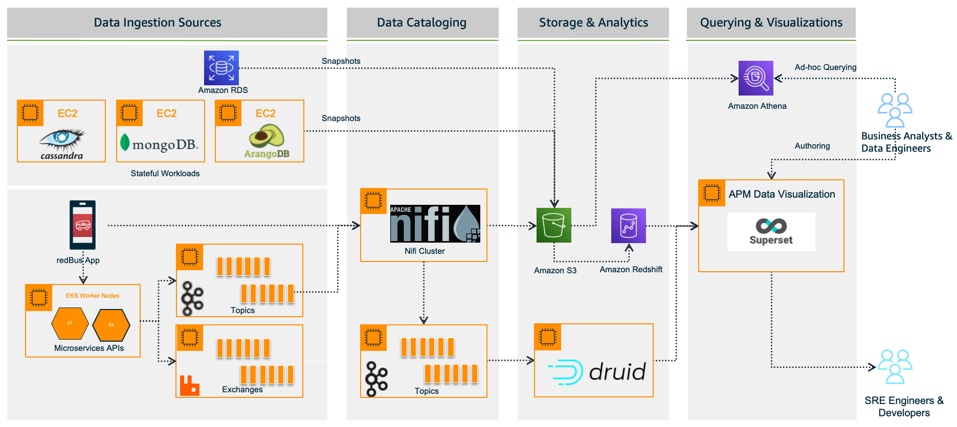
redBus relies heavily on making data-driven decisions at every level, from its traveler journey tracking, forecasting demand during high traffic, identifying and addressing bottlenecks in their bus operators signup process, and more. As redBus’s business started growing in terms of the number of cities and countries they operated in and the number of bus operators and travelers using the service in each city, the amount of incoming data also increased. The need to access and analyze the data in one place required them to build their own data platform, as shown in the following diagram.

redBus data platform 1.0

In the following sections, we look at each component in more detail.

Data ingestion sources

With the data platform 1.0, the data is ingested from various sources:

  • Real time – The real-time data flows from redBus mobile apps, the backend microservices, and when a passenger, bus operator, or application does any operation like booking bus tickets, searching the bus inventory, uploading a KYC document, and more
  • Batch mode – Scheduled jobs fetch data from multiple persistent data stores like Amazon Relational Database Service (Amazon RDS), where the OLTP data from all its applications are stored, Apache Cassandra clusters, where the bus inventory from various operators is stored, Arango DB, where the user identity graphs are stored, and more

Data cataloging

The real-time data is ingested into their self-managed Apache Nifi clusters, an open-source data platform that is used to clean, analyze, and catalog the data with its routing capabilities before sending the data to its destination.

Storage and analytics

redBus uses the following services for its storage and analytical needs:

  • Amazon Simple Storage Service (Amazon S3), an object storage service that provides the foundation for their data lake because of its virtually unlimited scalability and higher durability. Real-time data flows from Apache Druid and data from the data stores flow at regular intervals based on the schedules.
  • Apache Druid, an OLAP-style data store (data flows via Kafka Druid data loader), which computes facts and metrics against various dimensions during the data loading process.
  • Amazon Redshift, a cloud data warehouse service that helps you analyze exabytes of data and run complex analytical queries. redBus uses Amazon Redshift to store the processed data from Amazon S3 and the aggregated data from Apache Druid.

Querying and visualization

To make redBus as data-driven as possible, they ensured that the data is accessible to their SRE engineers, data engineers, and business analysts via a visualization layer. This layer features dashboards being served using Apache SuperSet, an open-source data visualization application, and Amazon Athena, an interactive query service to analyze data in Amazon S3 using standard SQL for ad hoc querying requirements.

The challenges

Initially, redBus handled data that was being ingested at the rate of 10 million events per day. Over time, as its business started growing, so did the data volume (from gigabytes to terabytes to petabytes), data ingestion per day (from 10 million to 320 million events), and its business intelligence dashboard needs. Soon after, they started facing challenges with their self-managed Superset’s BI capabilities, and the increased operational complexities.

Limited BI capabilities

redBus encountered the following BI limitations:

  • Inability to create visualizations from multiple data sources – Superset doesn’t allow creating visualizations from multiple tables within its data exploration layer. redBus data engineers had to have the tables joined beforehand at the data source level itself. In order to create a 360-degree view for redBus’s business stakeholders, it became inconvenient for data engineers to maintain multiple tables supporting the visualization layer.
  • No global filter for visuals in a dashboard – A global or primary filter across visuals in a dashboard is not supported in Superset. For example, consider there are visuals like Sales Wins by Region, YTD Revenue Realized by Region, Sales Pipeline by Region, and more in a dashboard, and a filter Region is added to the dashboard with values like EMEA, APAC, and US. The filter Region will only apply to one of the visuals, not the entire dashboard. However, dashboard users expected filtering across the dashboard.
  • Not a business-user friendly tool – Superset is highly developer centric when it comes to customization. For example, if a redBus business analyst had to customize a timed refresh that automatically re-queries every slice on a dashboard according to a pre-set value, then the analyst has to update the dashboard’s JSON metadata field. Therefore, having knowledge of JSON and its syntax is mandatory for doing any customization on the visuals or dashboard.

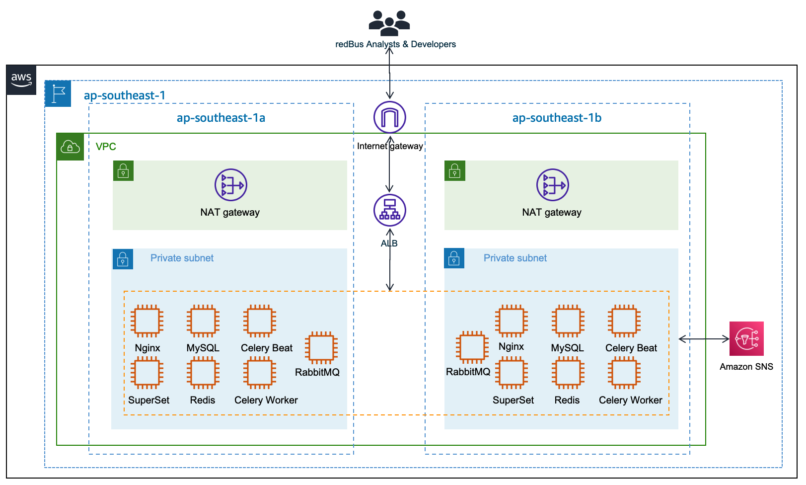
Increased operational cost

Although Superset is open source, which means there are no licensing costs, it also means there is more effort in maintaining all the components required for it to function as an enterprise-grade BI tool. redBus has deployed and maintained a web server (Nginx) fronted by an Application Load Balancer to do the load balancing; a metadata database server (MySQL) where Superset stores its internal information like users, slices, and dashboard definitions; an asynchronous task queue (Celery) for supporting long-running queries; a message broker (RabbitMQ); and a distributed caching server (Redis) for caching the results, charting data, and more on Amazon Elastic Compute Cloud (Amazon EC2) instances. The following diagram illustrates this architecture.

Apache Superset Deploment at redBus

redBus’s DevOps team had to do the heavy lifting of provisioning the infrastructure, taking backups, scaling the components manually as needed, upgrading the components individually, and more. It also required a Python web developer to be around for making the configurational changes so all the components work together seamlessly. All these manual operations increased the total cost of ownership for redBus.

Journey towards QuickSight

redBus started exploring BI solutions primarily around a couple of its dashboarding requirements:

  • BI dashboards for business stakeholders and analysts, where the data is sourced via Amazon S3 and Amazon Redshift.
  • A real-time application performance monitoring (APM) dashboard to help their SRE engineers and developers identify the root cause of an issue in their microservices deployment so they can fix the issues before they affect their customer’s experience. In this case, the data is sourced via Druid.

QuickSight fit into most of redBus’s BI dashboard requirements, and in no time their data platform team started with a proof of concept (POC) for a couple of their complex dashboards. At the end of the POC, which spanned a month’s time, the team shared their findings.

First, QuickSight is rich in BI capabilities, including the following:

  • It’s a self-service BI solution with drag-and-drop features that could help redBus analysts comfortably use it without any coding efforts.
  • Visualizations from multiple data sources in a single dashboard could help redBus business stakeholders get a 360-degree view of sales, forecasting, and insights in a single pane of glass.
  • Cascading filters across visuals and across sheets in a dashboard are much-needed features for redBus’s BI requirements.
  • QuickSight offers Excel-like visuals—tables with calculations, pivot tables with cell grouping, and styling are attractive for the viewers.
  • The Super-fast, Parallel, In-memory Calculation Engine (SPICE) in QuickSight could help redBus scale to hundreds of thousands of users, who can all simultaneously perform fast interactive analysis across a wide variety of AWS data sources.
  • Off-the-shelf ML insights and forecasting at no additional cost would allow redBus’s data science team to focus on ML models besides sales forecasting and similar models.
  • Built-in row-level security (RLS) could allow redBus to grant filtered access for their viewers. For example, redBus has many business analysts who manage different countries. With RLS, each business analyst only sees data related to their assigned country within a single dashboard.
  • redBus uses OneLogin as its identity provider, which supports Security Assertion Markup Language 2.0 (SAML 2.0). With the help of identity federation and single sign-on support from QuickSight, redBus could provide a simple onboarding flow for their QuickSight users.
  • QuickSight offers built-in alerts and email notification capabilities.

Secondly, QuickSight is a fully managed, cloud-native, serverless BI service offering from AWS, with the following features:

  • redBus engineers don’t need to focus on the heavy lifting of provisioning, scaling, and maintaining their BI solution on EC2 instances.
  • QuickSight offers native integration with AWS services like Amazon Redshift, Amazon S3, and Athena, and other popular frameworks like Presto, Snowflake, Teradata, and more. QuickSight connects to most of the data sources that redBus already has except Apache Druid, because native integration with Druid was not available as of December 2022. For a complete list of the supported data sources, see Supported data sources.
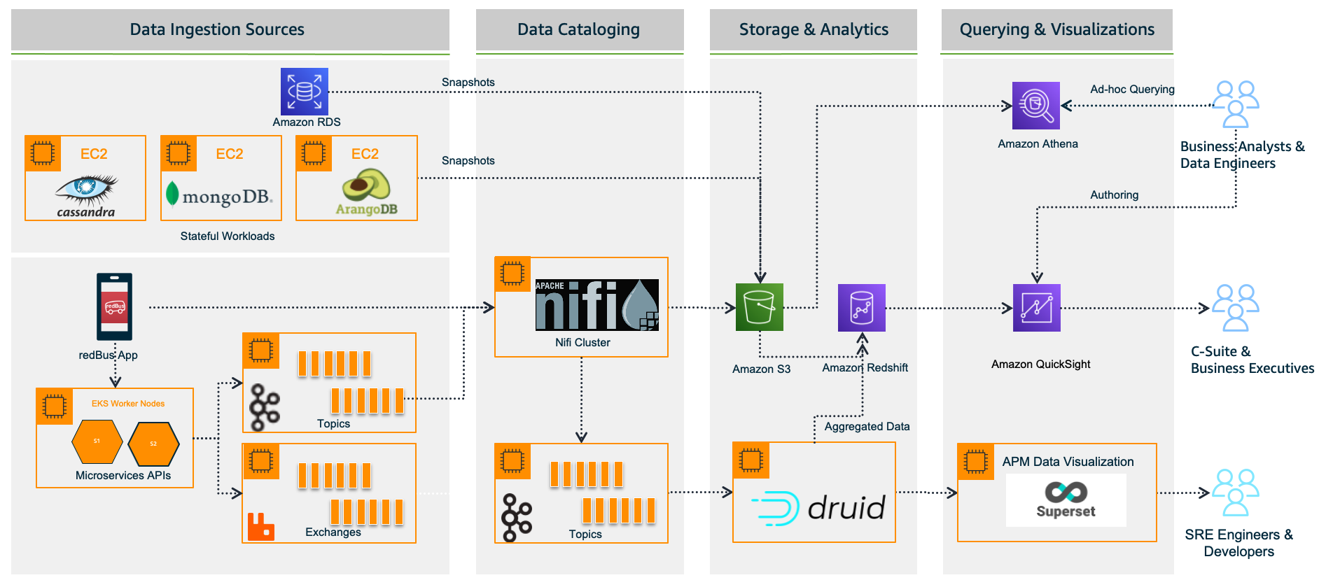
The outcome

Considering all the rich features and lower total cost of ownership, redBus chose QuickSight for their BI dashboard requirements. With QuickSight, redBus’s data engineers have built a number of dashboards in no time to give insights from petabytes of data to business stakeholders and analysts. The redBus data highway evolved to bring business intelligence to a much wider audience in their organization, with better performance and faster time-to-value. As of November 2022, it combines QuickSight for business users and Superset for real-time APM dashboards (at the time of writing, QuickSight doesn’t offer a native connector to Druid), as shown in the following diagram.

redBus data platform 2.0

Sales anomaly detection dashboard

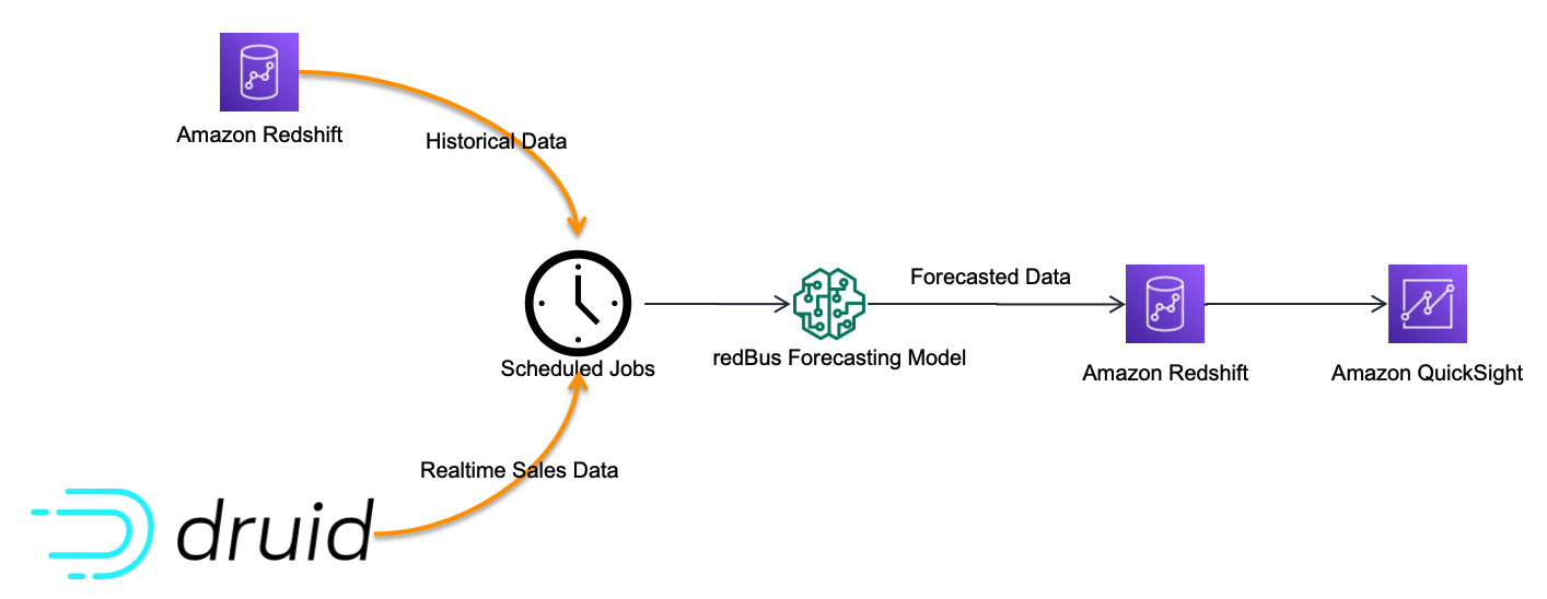
Although there are many dashboards that redBus deployed to production, sales anomaly detection is one of the interesting dashboards that redBus built. It uses redBus’s proprietary sales forecasting model, which in turn is sourced by historical sales data from Amazon Redshift tables and real-time sales data from Druid tables, as shown in the following figure.

Sales anomaly detection data flow

At regular intervals, the scheduled jobs feed the redBus forecasting model with real-time and historical sales data, and then the forecasted data is pushed into an Amazon Redshift table. The sales anomaly detection dashboard in QuickSight is served by the resultant Amazon Redshift table.

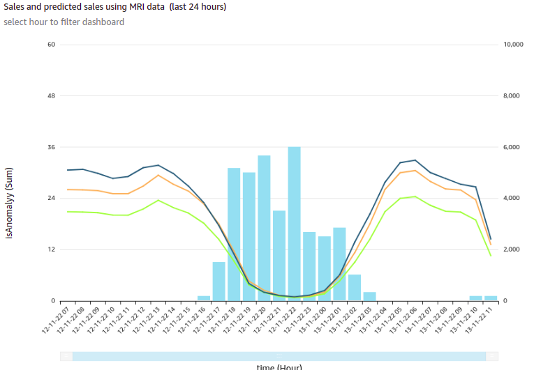
The following is one of the visuals from the sales anomaly detection dashboard. It’s built using a line chart representing hourly actual sales, predicted sales, and an alert threshold for a time series for a particular business cohort in redBus.

Sales and Predicted Sales for a particular cohort

In this visual, each bar represents the number of sales anomalies triggered at a particular point in the time series.

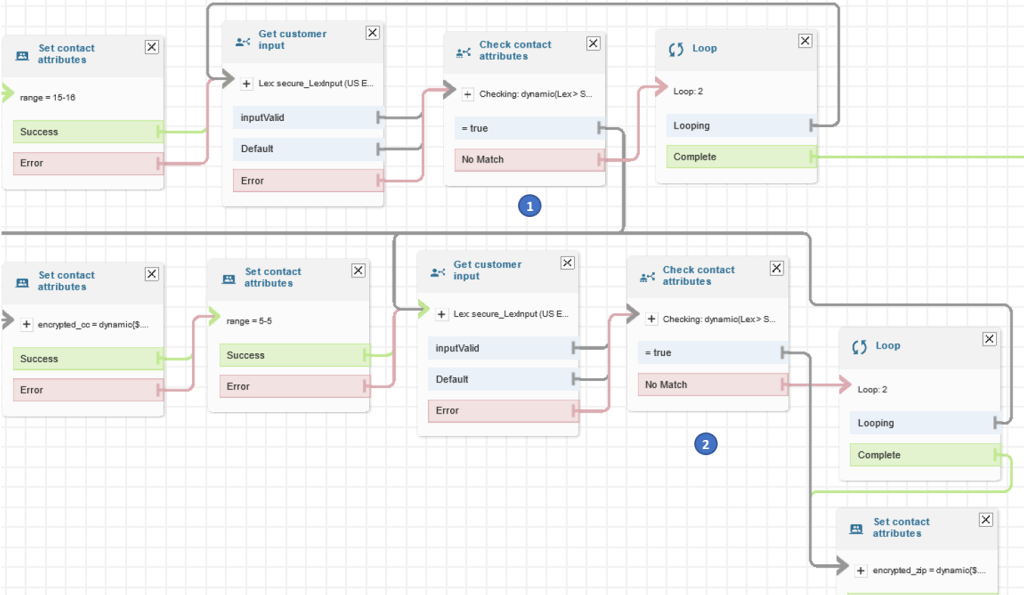
redBus’s analysts could further drill down to the sales details and anomalies at the minute level, as shown in the following diagram. This drill-down feature comes out of the box with QuickSight.

Drill-Down Chart - Sales and Predicted Sales for a particular cohort

For more details on adding drill-downs to QuickSight dashboard visuals, see Adding drill-downs to visual data in Amazon QuickSight.

Apart from the visuals, it has become one of viewers’ favorite dashboards at redBus due to the following notable features:

  • Because filtering across visuals is an out-of-the-box feature in QuickSight, a timestamp-based filter is added to the dashboard. This helps in filtering multiple visuals in the dashboard in a single click.
  • URL actions configured on the visuals help the viewers navigate to the context-sensitive in-house applications.
  • Email alerts configured on KPIs and Gauge visuals help the viewers get notifications on time.

Next steps

Apart from building new dashboards for their BI dashboard needs, redBus is taking the following next steps:

  • Exploring QuickSight Embedded Analytics for a couple of their application requirements to accelerate time to insights for users with in-context data visuals, interactive dashboards, and more directly within applications
  • Exploring QuickSight Q, which could enable their business stakeholders to ask questions in natural language and receive accurate answers with relevant visualizations that can help them gain insights from the data
  • Building a unified dashboarding solution using QuickSight covering all their data sources as integrations become available

Conclusion

In this post, we showed you how redBus built its data platform using various AWS services and Apache frameworks, the challenges the platform went through (especially in their BI dashboard requirements and challenges while scaling), and how they used QuickSight and lowered the total cost of ownership.

To know more about engineering at redBus, check out their medium blog posts. To learn more about what is happening in QuickSight or if you have any questions, reach out to the QuickSight Community, which is very active and offers several resources.


About the Authors


Author: Girish Chidanand
Girish Kumar Chidananda
works as a Senior Engineering Manager – Data Engineering at redBus, where he has been building various data engineering applications and components for redBus for the last 5 years. Prior to starting his journey in the IT industry, he worked as a Mechanical and Control systems engineer in various organizations, and he holds an MS degree in Fluid Power Engineering from University of Bath.


Author: Kayalvizhi Kandasamy
Kayalvizhi Kandasamy
works with digital-native companies to support their innovation. As a Senior Solutions Architect (APAC) at Amazon Web Services, she uses her experience to help people bring their ideas to life, focusing primarily on microservice architectures and cloud-native solutions using AWS services. Outside of work, she likes playing chess and is a FIDE rated chess player. She also coaches her daughters the art of playing chess, and prepares them for various chess tournaments.

How to encrypt sensitive caller voice input in Amazon Lex

Post Syndicated from Herbert Guerrero original https://aws.amazon.com/blogs/security/how-to-encrypt-sensitive-caller-authentication-voice-input-in-amazon-lex/

In the telecommunications industry, sensitive authentication and user data are typically received through mobile voice and keypads, and companies are responsible for protecting the data obtained through these channels. The increasing use of voice-driven interactive voice response (IVR) has resulted in a need to provide solutions that can protect user data that is gathered from mobile voice inputs. In this blog post, you’ll see how to protect a caller’s sensitive voice data that was captured through Amazon Lex by using data encryption implemented through AWS Lambda functions. The solution described in this post helps you to protect customer data received through voice channels from inadvertent or unknown access. The solution also includes decryption capabilities, which give an authorized administrator or operator the ability to decrypt user data from a Lambda console.

Solution overview

To demonstrate the IVR solution described in this post, a caller speaks two sensitive pieces of data—credit card number and zip code—from an Amazon Connect contact flow. The spoken values are encrypted and returned to the contact flow to be stored in contact attributes. The encrypted ciphertext is retained as a contact attribute for decryption purposes. Amazon CloudWatch Logs is enabled in the contact flow, but only the encrypted values are logged in log streams.

For this solution, conversation logs for this Amazon Lex bot are not enabled. An operator with assigned AWS Identity and Access Management (IAM) permissions can monitor the logged encrypted entries from CloudWatch Logs. For more information, see Working with log groups and log streams in the Amazon CloudWatch Logs User Guide.

Solution architecture

Figure 1 shows the overview of the solution described in this blog post.

Figure 1: Example of solution architecture

Figure 1: Example of solution architecture

Figure 1 shows the following high-level steps of the solution, and the number labels correspond to the following steps.

  1. A caller places an inbound call.
  2. An Amazon Connect contact flow leverages a Get customer input block, backed by an Amazon Lex bot, to prompt the caller for numerical data.
  3. The Amazon Lex bot invokes the Lambda function dev-encryption-core-EncryptFn.
  4. The Lambda function uses the AWS Encryption SDK to encrypt the caller’s plain text data.
  5. The AWS Encryption SDK obtains encryption keys from AWS Key Management Service (AWS KMS).
  6. The caller’s data is encrypted by using the AWS KMS keys obtained from AWS KMS.
  7. The Lambda function appends the encrypted data to the Amazon Lex bot session attributes.
  8. Amazon Lex returns the fully encrypted data back to Amazon Connect.

Overview of a contact flow

Figure 2: Contact flow captures input values using Amazon Lex and returns their encrypted values

Figure 2: Contact flow captures input values using Amazon Lex and returns their encrypted values

Figure 2 shows an overview of the contact flow, which has two main steps:

  1. The first numerical data (in this example, an encrypted credit card number value) is stored in contact attributes.
  2. The second numerical data (in this example, an encrypted zip code value) is stored in contact attributes.

Prerequisites

This solution uses the following AWS services:

The following need to be installed in your local machine:

To implement the solution in this post, you first need the Amazon Connect instance prerequisite in place.

To set up the Amazon Connect instance (if none exists)

  1. Create an Amazon Connect instance with a claimed phone number and a configured Amazon Connect user linked to a basic routing profile. For more information about setting up a contact center, see Set up your contact center in the Amazon Connect Administrator Guide.
  2. Assign the CallCenterManager or Admin security profile to an Amazon Connect user.
  3. In the newly created Amazon Connect instance, under the Overview section, find the access URL with the format
    https://<aliasname>.awsapps.com/connect/login

    • Make note of the access URL, which you will use later to log in to the Amazon Connect Dashboard.
  4. Log in to your Amazon Connect instance with a Connect user that has Admin or CallCenterManager permissions.

Solution procedures

This solution includes the following procedures:

  1. Clone the project or download the solution zip file.
  2. Create AWS resources needed for encryption and decryption.
  3. Configure the Amazon Lex bot in Amazon Connect.
  4. Create the contact flow in Amazon Connect.
  5. Validate the solution.
  6. Decrypt the collected data.

To clone or download the solution

  • Log in to the GitHub repo.
  • Clone or download the solution files to your local machine.

The downloaded file contains the artifacts needed for the deployment.

To create AWS resources needed for encryption and decryption

  1. From the command line, change directory to the project’s root directory.
  2. Run npm install.
  3. Run npm run build to transpile TypeScript to JavaScript and package code and its dependencies before deploying to AWS.
  4. Run cdk deploy CoreStack.

To configure the Amazon Lex bot in your Amazon Connect instance

  1. In the Amazon Connect console, choose Contact flows and scroll to the Amazon Lex section.
    Figure 3: Select Contact flows

    Figure 3: Select Contact flows

  2. From the Bot menu, select secure_LexInput(Classic). Then select +Add Amazon Lex Bot.
    Figure 4: Configure the Amazon Lex bot to Amazon Connect

    Figure 4: Configure the Amazon Lex bot to Amazon Connect

To import contact flow into Amazon Connect

  1. In the Amazon Connect console, choose Overview, and then choose Login as administrator.
  2. From the Routing menu on the left side, choose Contact flows to show the list of contact flows.
  3. Choose Create Contact flow.
  4. Choose the arrow to the right of the Save button and choose Import flow (beta). This imports the contact flow that you previously downloaded in the procedure To clone or download the solution.

    The contact flow already has the Amazon Lex bot configured.

    Figure 5: Select Import flow (beta)

    Figure 5: Select Import flow (beta)

  5. In the upper right corner of the contact flow, choose Save, and then choose OK to save the changes.
  6. Choose Publish to make the contact flow ready for use during the validation steps.
  7. (Optional) Claim a phone number (if none is available), using the following steps:
    1. In the Connect Dashboard, on the navigation menu, choose Channels, and then choose Phone numbers.
    2. On the right side of the page, choose Claim a number.
    3. Select the DID (Direct Inward Dialing) tab. Use the drop-down arrow to choose your country/region. When numbers are returned, choose one.
    4. Write down the phone number. You call it later in this post.
  8. (Optional) On the Edit Phone number page, in the Description box, you can type a note if desired.
  9. To assign the contact flow to your claimed phone number, for Contact flow / IVR, choose the drop-down arrow, and then choose Secure_Lex_Input.
  10. Choose Save.
    Figure 6: Under Contact flow / IVR, select the imported contact flow

    Figure 6: Under Contact flow / IVR, select the imported contact flow

For more information, see Set up phone numbers for your contact center in the Amazon Connect Administrator Guide.

To validate the solution

  1. Dial the test phone number to go through the voice prompt flow.
  2. When prompted, speak a 16-digit credit card number (you have a maximum of two retries), then speak a 5-digit zip code (also a maximum of two retries).
  3. After you complete your test call, review the log streams in Amazon CloudWatch Logs to confirm that the digits that you entered are now encrypted and stored as a contact attribute. The two entered values zipcode and creditcard are stored in contact attributes. Both are encrypted.
    Figure 7: Sample log showing encrypted values for zipcode and creditcard

    Figure 7: Sample log showing encrypted values for zipcode and creditcard

  4. Log in to your Amazon Connect Dashboard as a Supervisor. The URL is provided after the connect instance has been created. In the navigation menu, choose Contact search.
    Figure 8: Choose Contact search to look for the call information

    Figure 8: Choose Contact search to look for the call information

  5. Locate your inbound call on the Contact search list. Note that it can take up to 60 seconds for data to appear in the Contact search list.
  6. Select the Contact ID for your call.
    Figure 9: The Contact search showing the contact details for your test call

    Figure 9: The Contact search showing the contact details for your test call

  7. Copy the encrypted values for creditcard and zipcode and make note of them; you will use these values in the next procedure.
    Figure 10: Contact attributes stored in a contact flow are registered as part of the contact details

    Figure 10: Contact attributes stored in a contact flow are registered as part of the contact details

To decrypt the collected data

  1. In the AWS Lambda console, choose Functions.
  2. Use the Search bar to look for the dev-encryption-core-DecryptFn Lambda function, and then select the name link to open it.
  3. Under folder encryption-master, open the test folder. Under the tab \events, locate the file decrypt.json.
  4. Use the following steps to create a sample test event in the console by using the contents from decrypt.json. For more details, see Testing Lambda functions in the console.
    1. Choose the down arrow on the right side of Test.
    2. Choose Configure test event.
    3. Choose Create new test event.
    4. For Event name, enter decryptTest.
    5. Paste the contents from decrypt.json.
      {
          "Details": {
              "Parameters": {
                  "encrypted": "<encrypted-value-here>"
              }
          }
      }

    6. Choose Save.
  5. Use the encrypted values saved in the Validate a solution procedure and replace the ones in the recently created test event.
    Figure 11: Replace the creditcard or zipCode values with the ones from the Contact Search page

    Figure 11: Replace the creditcard or zipCode values with the ones from the Contact Search page

  6. Choose Test. The output from the test shows the values decrypted by the Lambda function. This is shown in Figure 12 under the Execution result tab.
    Figure 12: Result from the decryption operation

    Figure 12: Result from the decryption operation

Note: Make sure that only the appropriate authorized administrator or operator, application, or AWS service is able to invoke the decryption Lambda function.

You have now successfully implemented the solution by encrypting and decrypting the voice input of your test call, which you collected through Amazon Lex.

Cleanup

To avoid incurring future charges, follow these steps to clean up the deployed resources that you created when implementing this solution.

To delete the Amazon Connect instance

  1. In the Amazon Connect console, under Instance alias, select the name of the Amazon Connect instance, and choose Delete.
  2. When prompted, type the name of the instance, and then choose Delete.

To delete the Amazon Lex bot

  1. In the Amazon Lex console, choose the bot that you created in the To configure the Amazon Lex bot procedure.
  2. Choose Delete, and then choose Continue.

To delete the AWS CloudFormation stack

  1. In the AWS CloudFormation console, on the Stacks page, select the stack you created in the procedure To create AWS resources needed for encryption and decryption.
  2. In the stack details pane, choose Delete.
  3. Choose Delete stack when prompted. This deletes the Amazon S3 bucket, IAM roles and AWS Lambda functions you created for testing. This will also schedule a deletion date on the AWS KMS key.

Conclusion

In this post, you learned how an Amazon Connect contact flow can collect voice inputs from a caller by using Amazon Lex, and how you can encrypt these inputs by using your own AWS KMS key. This solution can help improve the security of voice input that is collected through Amazon Connect. For cost information, see the Amazon Connect pricing page.

For more information, see the blog post Creating a secure IVR solution with Amazon Connect and the topic Encrypt customer input (using OpenSSL) in the Amazon Connect Administrator Guide. As previously mentioned, the increasing use of voice-driven IVR has resulted in a need to provide solutions that can protect user data gathered from mobile voice inputs.

Additional resources include the AWS Lambda Developer Guide, the Amazon Lex Developer Guide, the Amazon Connect Administrator Guide, the AWS Nodejs SDK, and the AWS SDK for Python (Boto3).

If you need help with setting up this solution, you can get assistance from AWS Professional Services. You can also seek assistance from Amazon Connect partners available worldwide.

 
If you have feedback about this post, submit comments in the Comments section below. If you have questions about this post, contact AWS Support.

Want more AWS Security news? Follow us on Twitter.

Herbert Guerrero

Herbert Guerrero

Herbert is a Senior Proserve Consultant for Connect. He enjoys designing and developing high-usability and scalable solutions. Understanding success criteria helps Herbert work backwards and deliver well-architected solutions. His engineering background informs the way he engages with customers’ mental models of what their solutions should look like.

Ed Valdez

Ed Valdez

Ed is a Specialty Consultant with Amazon Web Services. As a software development professional with over 23 years of experience, he specializes on designing and delivering customer-centric solutions within the contact center domain.

Streaming the AWS Wickr desktop client with Amazon AppStream 2.0

Post Syndicated from Charles H. original https://aws.amazon.com/blogs/architecture/streaming-the-aws-wickr-desktop-client-with-amazon-appstream-2-0/

Amazon Web Services (AWS) customers using AWS Wickr who want to find a way to access their AWS Wickr Windows desktop client though a web browser, can use Amazon AppStream 2.0 to stream the application through to their users.

Using this architecture, you can provide lightweight access to the AWS Wickr desktop client for users that cannot install it onto their local device. By using AppStream 2.0, you can focus on managing your AWS Wickr network while AppStream 2.0 manages the AWS resources required to host and run the application, scaling automatically and providing on-demand access to your users.

If you want to ensure that AWS Wickr user data persists between streaming sessions, you can make use of AppStream 2.0 user persistence to securely save user data (including AWS Wickr client data) to Amazon Simple Storage Service (Amazon S3).

In this post, we discuss how to build an AppStream 2.0 image for AWS Wickr on Windows, enable persistence for users, and deploy a stack.

Solution overview

These steps will illustrate deploying an AppStream 2.0 Windows Image Builder to a single availability zone. Then we deploy an AppStream 2.0 fleet with internet access and user data persistence to three availability zones for high availability.

Review the Regions and Availability Zones documentation and the AWS Regional Services List to choose the best Region for your deployment, as well as the networking and bandwidth requirements for User Connections to Amazon AppStream 2.0.

AWS Wickr with Amazon AppStream 2.0 Architecture

Figure 1. AWS Wickr with Amazon AppStream 2.0 Architecture

Cost

The costs associated with using AWS services when deploying AppStream 2.0 and AWS Wickr in your AWS account can be estimated on the pricing pages for the services used.

Walkthrough

This walkthrough takes you from installing the AWS Wickr for Windows desktop client onto an AppStream 2.0 Image Builder, to configuring the client for persistence, and finally to deploying a fleet and stack for your users to consume:

  1. Install AWS Wickr for Windows client onto your AppStream 2.0 Windows Image Builder.
  2. Configure the client using the Image Assistant to set up user data and settings persistence.
  3. Create an on-demand instance streaming fleet.
  4. Create a user stack and enable user data and settings persistence.
  5. Create a user pool.
  6. Test your streaming application and prove data persistence.

Prerequisites

You should have the following prerequisites:

  • Familiarity with AppStream 2.0 and an existing AWS Wickr account with associated credentials. Currently, it is not possible for an AWS Wickr user to register their account over AppStream 2.0.
  • An AWS account with access to AppStream 2.0. Instructions for setting up an AWS account can be found at Setting Up for Amazon AppStream 2.0.
  • A running AppStream 2.0 image builder, based on the WinServer2019-10-05-2022 base image with the AWS Wickr for Windows client installer downloaded to it.
  • An up-to-date Google Chrome browser (if you want to use your device’s webcam).

Install AWS Wickr

AppStream 2.0 uses Amazon Elastic Compute Cloud (Amazon EC2) instances to stream applications. You launch instances from base images, called image builders. In this step you will install the AWS Wickr client onto your image builder before moving on to configuration.

  1. Connect to your image builder as an Administrator.
  2. Run the AWS Wickr installer and carry out the following steps:
    1. On the Welcome to the AWS Wickr Setup Wizard prompt, choose Next.
    2. For Installation Type, choose Everybody (all users).
    3. Choose Next to accept the default installation folder.
    4. Choose Install.
  3. Once the AWS Wickr client has finished installing, uncheck Launch Wickr on the final screen, and then choose Finish.

Run the Image Assistant

To create your own custom image, connect to an image builder instance, install and configure your applications for streaming with guidance from the Image Assistant, and then create your image by creating a snapshot of the image builder instance:

  1. Run the Image Assistant shortcut found on the desktop.
  2. Under 1. ADD APPS, choose Add App.
  3. Choose Program Files, Amazon Web Services, Wickr, and AWS Wickr.
  4. Scroll to the bottom, choose the Wickr application, and then choose Open.
  5. In the pop-up that appears, customize the Name and Display Name (if needed), and then in the Launch Parameters box, enter -datalocation “C:\Users\%username%” (Figure 2).
    Updating Launch Parameters

    Figure 2. Updating Launch Parameters

    Note: If you want to mask the name of the application within the URL used for streaming, replace the Display Name field text with something else.

  6. Choose Save.
  7. Wickr will now appear as an app on the Image Assistant screen. Choose Next.
  8. Under the 2. CONFIGURE APPS stage, follow the instructions from 1-5, choose Save settings, and choose Next (Figure 3).

    Configuring the Application with Image Assistant

    Figure 3. Configuring the Application with Image Assistant

  9. Under the 3. TEST stage, carry out steps 1-3.
  10. Under the 4. OPTIMIZE stage, select Launch.
  11. As instructed, once the app has launched successfully, select Continue and wait for the app to be optimized.
  12. Under the 5. CONFIGURE IMAGE stage, give the image that will be created a Name, Display name, and Description.
  13. Choose the Always use latest agent version checkbox. This ensures that new image builders or fleet instances that are launched from your image always use the latest AppStream 2.0 agent version, and then select Next (Figure 4).

    Finalizing the Application Image

    Figure 4. Finalizing the Application Image

  14. Under the 6. REVIEW stage, select Disconnect and Create Image. Your session will be terminated while your image is being created.

Create an AppStream 2.0 fleet

With AppStream 2.0, you create fleet instances and stacks as part of the process of streaming applications. A fleet consists of streaming instances that run the image that you specify.

  1. Return to the AppStream 2.0 management console.
  2. Choose Fleets from the menu on the left.
  3. Choose your Fleet type (this demonstration uses On-Demand) and choose Next.
  4. Give the Fleet a Name, Display name, and a Description.
    Note: If you wish to mask the name of the fleet within the URL used for streaming, replace the Name and Display name section with something else.
  5. Choose your Fleet instance type (this walkthrough uses a general purpose stream.standard.large instance type).
  6. Adjust the Fleet capacity as required, leave the other sections as they’re displayed by default, and choose Next.
  7. On the Choose an Image screen, choose the image you created earlier.
  8. On the Configure network screen, choose Enable default internet access and choose your VPC, along with three subnets that you will deploy into. Finally, choose the Security group that you will use to restrict access (the default is to allow access from all IPs). Choose Next.
  9. Review your settings and then choose Create fleet.

Create an AppStream 2.0 stack

A stack consists of an associated fleet, user access policies, and storage configurations. In this step, you will create a stack, enable application settings persistence, and associate the stack with the fleet you provisioned previously.

  1. From the menu in the AppStream 2.0 management console, choose Stacks.
  2. Choose Create Stack.
  3. Give the stack a Name, and optionally a Display name and Description.
  4. Leave all other options as they’re displayed by default and choose Next.
  5. In the Enable storage window, ensure that Enable home folders is selected, leave all the settings as they are, and choose Next.
  6. In the Edit user settings section, modify the copy and paste functionality to your requirements, and ensure that Enable application settings persistence is selected. Choose Next.
  7. Review your configuration and choose Create stack.
  8. You will now be presented with an overview of the stack you have created. Choose the Action dropdown list and choose Associate fleet.
  9. From the dropdown list, choose the fleet that you previously provisioned and choose Associate.

Create an AppStream 2.0 user pool

Users can access application stacks through a persistent URL and login credentials by using their email address and a password that they choose. In this step, you will create a user and assign it to a stack so you can access your AppStream 2.0 streaming session.

  1. Choose User pool.
  2. Choose Create user.
  3. Enter an email address, first name, and last name, and then choose Create User.
  4. In the User pool window, choose the User and then choose Action.
  5. Choose Assign stack, choose the newly created stack, and choose Send email notification to user.
  6. Choose Assign stack.
  7. You will receive two emails. Follow the instructions on the one titled Start accessing your apps using AppStream 2.0 to access your app.

Launch your AppStream 2.0 streaming session

In this step, you will use the user created earlier to log in to an AppStream 2.0 streaming session. You will then prove AWS Wickr user data persistence by exiting and logging back into your session.

Note: You will only be able to launch your session once your fleet has been provisioned. This can take around 15-20 minutes.

  1. Choose the login page link from the email you received in the previous section and log in.
  2. You will be presented with the AWS Wickr client icon. Choose it to start your session.
  3. Log in to the AWS Wickr client with your credentials.
  4. As you have application persistence enabled, you can close the tab and the session will pick up from where you left it when you log back in (Figure 5).
Accessing the Streaming Application

Figure 5. Accessing the Streaming Application

Cleanup

To avoid incurring future charges, delete the stack, user, fleet, custom image, and image builder that you have created.

Conclusion

In this post, we demonstrated how customers can take advantage of AppStream 2.0 as a managed service to enable the provisioning of AWS Wickr clients for users, with persistence between sessions, through a web browser.

How BookMyShow saved 80% in costs by migrating to an AWS modern data architecture

Post Syndicated from Mahesh Vandi Chalil original https://aws.amazon.com/blogs/big-data/how-bookmyshow-saved-80-in-costs-by-migrating-to-an-aws-modern-data-architecture/

This is a guest post co-authored by Mahesh Vandi Chalil, Chief Technology Officer of BookMyShow.

BookMyShow (BMS), a leading entertainment company in India, provides an online ticketing platform for movies, plays, concerts, and sporting events. Selling up to 200 million tickets on an annual run rate basis (pre-COVID) to customers in India, Sri Lanka, Singapore, Indonesia, and the Middle East, BookMyShow also offers an online media streaming service and end-to-end management for virtual and on-ground entertainment experiences across all genres.

The pandemic gave BMS the opportunity to migrate and modernize our 15-year-old analytics solution to a modern data architecture on AWS. This architecture is modern, secure, governed, and cost-optimized architecture, with the ability to scale to petabytes. BMS migrated and modernized from on-premises and other cloud platforms to AWS in just four months. This project was run in parallel with our application migration project and achieved 90% cost savings in storage and 80% cost savings in analytics spend.

The BMS analytics platform caters to business needs for sales and marketing, finance, and business partners (e.g., cinemas and event owners), and provides application functionality for audience, personalization, pricing, and data science teams. The prior analytics solution had multiple copies of data, for a total of over 40 TB, with approximately 80 TB of data in other cloud storage. Data was stored on‑premises and in the cloud in various data stores. Growing organically, the teams had the freedom to choose their technology stack for individual projects, which led to the proliferation of various tools, technology, and practices. Individual teams for personalization, audience, data engineering, data science, and analytics used a variety of products for ingestion, data processing, and visualization.

This post discusses BMS’s migration and modernization journey, and how BMS, AWS, and AWS Partner Minfy Technologies team worked together to successfully complete the migration in four months and saving costs. The migration tenets using the AWS modern data architecture made the project a huge success.

Challenges in the prior analytics platform

  • Varied Technology: Multiple teams used various products, languages, and versions of software.
  • Larger Migration Project: Because the analytics modernization was a parallel project with application migration, planning was crucial in order to consider the changes in core applications and project timelines.
  • Resources: Experienced resource churn from the application migration project, and had very little documentation of current systems.
  • Data : Had multiple copies of data and no single source of truth; each data store provided a view for the business unit.
  • Ingestion Pipelines: Complex data pipelines moved data across various data stores at varied frequencies. We had multiple approaches in place to ingest data to Cloudera, via over 100 Kafka consumers from transaction systems and MQTT(Message Queue Telemetry Transport messaging protocol) for clickstreams, stored procedures, and Spark jobs. We had approximately 100 jobs for data ingestion across Spark, Alteryx, Beam, NiFi, and more.
  • Hadoop Clusters: Large dedicated hardware on which the Hadoop clusters were configured incurring fixed costs. On-premises Cloudera setup catered to most of the data engineering, audience, and personalization batch processing workloads. Teams had their implementation of HBase and Hive for our audience and personalization applications.
  • Data warehouse: The data engineering team used TiDB as their on-premises data warehouse. However, each consumer team had their own perspective of data needed for analysis. As this siloed architecture evolved, it resulted in expensive storage and operational costs to maintain these separate environments.
  • Analytics Database: The analytics team used data sourced from other transactional systems and denormalized data. The team had their own extract, transform, and load (ETL) pipeline, using Alteryx with a visualization tool.

Migration tenets followed which led to project success:

  • Prioritize by business functionality.
  • Apply best practices when building a modern data architecture from Day 1.
  • Move only required data, canonicalize the data, and store it in the most optimal format in the target. Remove data redundancy as much possible. Mark scope for optimization for the future when changes are intrusive.
  • Build the data architecture while keeping data formats, volumes, governance, and security in mind.
  • Simplify ELT and processing jobs by categorizing the jobs as rehosted, rewritten, and retired. Finalize canonical data format, transformation, enrichment, compression, and storage format as Parquet.
  • Rehost machine learning (ML) jobs that were critical for business.
  • Work backward to achieve our goals, and clear roadblocks and alter decisions to move forward.
  • Use serverless options as a first option and pay per use. Assess the cost and effort for rearchitecting to select the right approach. Execute a proof of concept to validate this for each component and service.

Strategies applied to succeed in this migration:

  • Team – We created a unified team with people from data engineering, analytics, and data science as part of the analytics migration project. Site reliability engineering (SRE) and application teams were involved when critical decisions were needed regarding data or timeline for alignment. The analytics, data engineering, and data science teams spent considerable time planning, understanding the code, and iteratively looking at the existing data sources, data pipelines, and processing jobs. AWS team with partner team from Minfy Technologies helped BMS arrive at a migration plan after a proof of concept for each of the components in data ingestion, data processing, data warehouse, ML, and analytics dashboards.
  • Workshops – The AWS team conducted a series of workshops and immersion days, and coached the BMS team on the technology and best practices to deploy the analytics services. The AWS team helped BMS explore the configuration and benefits of the migration approach for each scenario (data migration, data pipeline, data processing, visualization, and machine learning) via proof-of-concepts (POCs). The team captured the changes required in the existing code for migration. BMS team also got acquainted with the following AWS services:
  • Proof of concept – The BMS team, with help from the partner and AWS team, implemented multiple proofs of concept to validate the migration approach:
    • Performed batch processing of Spark jobs in Amazon EMR, in which we checked the runtime, required code changes, and cost.
    • Ran clickstream analysis jobs in Amazon EMR, testing the end-to-end pipeline. Team conducted proofs of concept on AWS IoT Core for MQTT protocol and streaming to Amazon S3.
    • Migrated ML models to Amazon SageMaker and orchestrated with Amazon MWAA.
    • Created sample QuickSight reports and dashboards, in which features and time to build were assessed.
    • Configured for key scenarios for Amazon Redshift, in which time for loading data, query performance, and cost were assessed.
  • Effort vs. cost analysis – Team performed the following assessments:
    • Compared the ingestion pipelines, the difference in data structure in each store, the basis of the current business need for the data source, the activity for preprocessing the data before migration, data migration to Amazon S3, and change data capture (CDC) from the migrated applications in AWS.
    • Assessed the effort to migrate approximately 200 jobs, determined which jobs were redundant or need improvement from a functional perspective, and completed a migration list for the target state. The modernization of the MQTT workflow code to serverless was time-consuming, decided to rehost on Amazon Elastic Compute Cloud (Amazon EC2) and modernization to Amazon Kinesis in to the next phase.
    • Reviewed over 400 reports and dashboards, prioritized development in phases, and reassessed business user needs.

AWS cloud services chosen for proposed architecture:

  • Data lake – We used Amazon S3 as the data lake to store the single truth of information for all raw and processed data, thereby reducing the copies of data storage and storage costs.
  • Ingestion – Because we had multiple sources of truth in the current architecture, we arrived at a common structure before migration to Amazon S3, and existing pipelines were modified to do preprocessing. These one-time preprocessing jobs were run in Cloudera, because the source data was on-premises, and on Amazon EMR for data in the cloud. We designed new data pipelines for ingestion from transactional systems on the AWS cloud using AWS Glue ETL.
  • Processing – Processing jobs were segregated based on runtime into two categories: batch and near-real time. Batch processes were further divided into transient Amazon EMR clusters with varying runtimes and Hadoop application requirements like HBase. Near-real-time jobs were provisioned in an Amazon EMR permanent cluster for clickstream analytics, and a data pipeline from transactional systems. We adopted a serverless approach using AWS Glue ETL for new data pipelines from transactional systems on the AWS cloud.
  • Data warehouse – We chose Amazon Redshift as our data warehouse, and planned on how the data would be distributed based on query patterns.
  • Visualization – We built the reports in Amazon QuickSight in phases and prioritized them based on business demand. We discussed with business users their current needs and identified the immediate reports required. We defined the phases of report and dashboard creation and built the reports in Amazon QuickSight. We plan to use embedded reports for external users in the future.
  • Machine learning – Custom ML models were deployed on Amazon SageMaker. Existing Airflow DAGs were migrated to Amazon MWAA.
  • Governance, security, and compliance – Governance with Amazon Lake Formation was adopted from Day 1. We configured the AWS Glue Data Catalog to reference data used as sources and targets. We had to comply to Payment Card Industry (PCI) guidelines because payment information was in the data lake, so we ensured the necessary security policies.

Solution overview

BMS modern data architecture

The following diagram illustrates our modern data architecture.

The architecture includes the following components:

  1. Source systems – These include the following:
    • Data from transactional systems stored in MariaDB (booking and transactions).
    • User interaction clickstream data via Kafka consumers to DataOps MariaDB.
    • Members and seat allocation information from MongoDB.
    • SQL Server for specific offers and payment information.
  2. Data pipeline – Spark jobs on an Amazon EMR permanent cluster process the clickstream data from Kafka clusters.
  3. Data lake – Data from source systems was stored in their respective Amazon S3 buckets, with prefixes for optimized data querying. For Amazon S3, we followed a hierarchy to store raw, summarized, and team or service-related data in different parent folders as per the source and type of data. Lifecycle polices were added to logs and temp folders of different services as per teams’ requirements.
  4. Data processing – Transient Amazon EMR clusters are used for processing data into a curated format for the audience, personalization, and analytics teams. Small file merger jobs merge the clickstream data to a larger file size, which saved costs for one-time queries.
  5. Governance – AWS Lake Formation enables the usage of AWS Glue crawlers to capture the schema of data stored in the data lake and version changes in the schema. The Data Catalog and security policy in AWS Lake Formation enable access to data for roles and users in Amazon Redshift, Amazon Athena, Amazon QuickSight, and data science jobs. AWS Glue ETL jobs load the processed data to Amazon Redshift at scheduled intervals.
  6. Queries – The analytics team used Amazon Athena to perform one-time queries raised from business teams on the data lake. Because report development is in phases, Amazon Athena was used for exporting data.
  7. Data warehouse – Amazon Redshift was used as the data warehouse, where the reports for the sales teams, management, and third parties (i.e., theaters and events) are processed and stored for quick retrieval. Views to analyze the total sales, movie sale trends, member behavior, and payment modes are configured here. We use materialized views for denormalized tables, different schemas for metadata, and transactional and behavior data.
  8. Reports – We used Amazon QuickSight reports for various business, marketing, and product use cases.
  9. Machine learning – Some of the models deployed on Amazon SageMaker are as follows:
    • Content popularity – Decides the recommended content for users.
    • Live event popularity – Calculates the popularity of live entertainment events in different regions.
    • Trending searches – Identifies trending searches across regions.

Walkthrough

Migration execution steps

We standardized tools, services, and processes for data engineering, analytics, and data science:

  • Data lake
    • Identified the source data to be migrated from Archival DB, BigQuery, TiDB, and the analytics database.
    • Built a canonical data model that catered to multiple business teams and reduced the copies of data, and therefore storage and operational costs. Modified existing jobs to facilitate migration to a canonical format.
    • Identified the source systems, capacity required, anticipated growth, owners, and access requirements.
    • Ran the bulk data migration to Amazon S3 from various sources.
  • Ingestion
    • Transaction systems – Retained the existing Kafka queues and consumers.
    • Clickstream data – Successfully conducted a proof of concept to use AWS IoT Core for MQTT protocol. But because we needed to make changes in the application to publish to AWS IoT Core, we decided to implement it as part of mobile application modernization at a later time. We decided to rehost the MQTT server on Amazon EC2.
  • Processing
  • Listed the data pipelines relevant to business and migrated them with minimal modification.
  • Categorized workloads into critical jobs, redundant jobs, or jobs that can be optimized:
    • Spark jobs were migrated to Amazon EMR.
    • HBase jobs were migrated to Amazon EMR with HBase.
    • Metadata stored in Hive-based jobs were modified to use the AWS Glue Data Catalog.
    • NiFi jobs were simplified and rewritten in Spark run in Amazon EMR.
  • Amazon EMR clusters were configured one persistent cluster for streaming the clickstream and personalization workloads. We used multiple transient clusters for running all other Spark ETL or processing jobs. We used Spot Instances for task nodes to save costs. We optimized data storage with specific jobs to merge small files and compressed file format conversions.
  • AWS Glue crawlers identified new data in Amazon S3. AWS Glue ETL jobs transformed and uploaded processed data to the Amazon Redshift data warehouse.
  • Datawarehouse
    • Defined the data warehouse schema by categorizing the critical reports required by the business, keeping in mind the workload and reports required in future.
    • Defined the staging area for incremental data loaded into Amazon Redshift, materialized views, and tuning the queries based on usage. The transaction and primary metadata are stored in Amazon Redshift to cater to all data analysis and reporting requirements. We created materialized views and denormalized tables in Amazon Redshift to use as data sources for Amazon QuickSight dashboards and segmentation jobs, respectively.
    • Optimally used the Amazon Redshift cluster by loading last two years data in Amazon Redshift, and used Amazon Redshift Spectrum to query historical data through external tables. This helped balance the usage and cost of the Amazon Redshift cluster.
  • Visualization
    • Amazon QuickSight dashboards were created for the sales and marketing team in Phase 1:
      • Sales summary report – An executive summary dashboard to get an overview of sales across the country by region, city, movie, theatre, genre, and more.
      • Live entertainment – A dedicated report for live entertainment vertical events.
      • Coupons – A report for coupons purchased and redeemed.
      • BookASmile – A dashboard to analyze the data for BookASmile, a charity initiative.
  • Machine learning
    • Listed the ML workloads to be migrated based on current business needs.
    • Priority ML processing jobs were deployed on Amazon EMR. Models were modified to use Amazon S3 as source and target, and new APIs were exposed to use the functionality. ML models were deployed on Amazon SageMaker for movies, live event clickstream analysis, and personalization.
    • Existing artifacts in Airflow orchestration were migrated to Amazon MWAA.
  • Security
    • AWS Lake Formation was the foundation of the data lake, with the AWS Glue Data Catalog as the foundation for the central catalog for the data stored in Amazon S3. This provided access to the data by various functionalities, including the audience, personalization, analytics, and data science teams.
    • Personally identifiable information (PII) and payment data was stored in the data lake and data warehouse, so we had to comply to PCI guidelines. Encryption of data at rest and in transit was considered and configured in each service level (Amazon S3, AWS Glue Data Catalog, Amazon EMR, AWS Glue, Amazon Redshift, and QuickSight). Clear roles, responsibilities, and access permissions for different user groups and privileges were listed and configured in AWS Identity and Access Management (IAM) and individual services.
    • Existing single sign-on (SSO) integration with Microsoft Active Directory was used for Amazon QuickSight user access.
  • Automation
    • We used AWS CloudFormation for the creation and modification of all the core and analytics services.
    • AWS Step Functions was used to orchestrate Spark jobs on Amazon EMR.
    • Scheduled jobs were configured in AWS Glue for uploading data in Amazon Redshift based on business needs.
    • Monitoring of the analytics services was done using Amazon CloudWatch metrics, and right-sizing of instances and configuration was achieved. Spark job performance on Amazon EMR was analyzed using the native Spark logs and Spark user interface (UI).
    • Lifecycle policies were applied to the data lake to optimize the data storage costs over time.

Benefits of a modern data architecture

A modern data architecture offered us the following benefits:

  • Scalability – We moved from a fixed infrastructure to the minimal infrastructure required, with configuration to scale on demand. Services like Amazon EMR and Amazon Redshift enable us to do this with just a few clicks.
  • Agility – We use purpose-built managed services instead of reinventing the wheel. Automation and monitoring were key considerations, which enable us to make changes quickly.
  • Serverless – Adoption of serverless services like Amazon S3, AWS Glue, Amazon Athena, AWS Step Functions, and AWS Lambda support us when our business has sudden spikes with new movies or events launched.
  • Cost savings – Our storage size was reduced by 90%. Our overall spend on analytics and ML was reduced by 80%.

Conclusion

In this post, we showed you how a modern data architecture on AWS helped BMS to easily share data across organizational boundaries. This allowed BMS to make decisions with speed and agility at scale; ensure compliance via unified data access, security, and governance; and to scale systems at a low cost without compromising performance. Working with the AWS and Minfy Technologies teams helped BMS choose the correct technology services and complete the migration in four months. BMS achieved the scalability and cost-optimization goals with this updated architecture, which has set the stage for innovation using graph databases and enhanced our ML projects to improve customer experience.


About the Authors

Mahesh Vandi Chalil is Chief Technology Officer at BookMyShow, India’s leading entertainment destination. Mahesh has over two decades of global experience, passionate about building scalable products that delight customers while keeping innovation as the top goal motivating his team to constantly aspire for these. Mahesh invests his energies in creating and nurturing the next generation of technology leaders and entrepreneurs, both within the organization and outside of it. A proud husband and father of two daughters and plays cricket during his leisure time.

Priya Jathar is a Solutions Architect working in Digital Native Business segment at AWS. She has more two decades of IT experience, with expertise in Application Development, Database, and Analytics. She is a builder who enjoys innovating with new technologies to achieve business goals. Currently helping customers Migrate, Modernise, and Innovate in Cloud. In her free time she likes to paint, and hone her gardening and cooking skills.

Vatsal Shah is a Senior Solutions Architect at AWS based out of Mumbai, India. He has more than nine years of industry experience, including leadership roles in product engineering, SRE, and cloud architecture. He currently focuses on enabling large startups to streamline their cloud operations and help them scale on the cloud. He also specializes in AI and Machine Learning use cases.

Genomics workflows, Part 4: processing archival data

Post Syndicated from Rostislav Markov original https://aws.amazon.com/blogs/architecture/genomics-workflows-part-4-processing-archival-data/

Genomics workflows analyze data at petabyte scale. After processing is complete, data is often archived in cold storage classes. In some cases, like studies on the association of DNA variants against larger datasets, archived data is needed for further processing. This means manually initiating the restoration of each archived object and monitoring the progress. Scientists require a reliable process for on-demand archival data restoration so their workflows do not fail.

In Part 4 of this series, we look into genomics workloads processing data that is archived with Amazon Simple Storage Service (Amazon S3). We design a reliable data restoration process that informs the workflow when data is available so it can proceed. We build on top of the design pattern laid out in Parts 1-3 of this series. We use event-driven and serverless principles to provide the most cost-effective solution.

Use case

Our use case focuses on data in Amazon Simple Storage Service Glacier (Amazon S3 Glacier) storage classes. The S3 Glacier Instant Retrieval storage class provides the lowest-cost storage for long-lived data that is rarely accessed but requires retrieval in milliseconds.

The S3 Glacier Flexible Retrieval and S3 Glacier Deep Archive provide further cost savings, with retrieval times ranging from minutes to hours. We focus on the latter in order to provide the most cost-effective solution.

You must first restore the objects before accessing them. Our genomics workflow will pause until the data restore completes. The requirements for this workflow are:

  • Reliable launch of the restore so our workflow doesn’t fail (due to S3 Glacier service quotas, or because not all objects were restored)
  • Event-driven design to mirror the event-driven nature of genomics workflows and perform the retrieval upon request
  • Cost-effective and easy-to-manage by using serverless services
  • Upfront detection of archived data when formulating the genomics workflow task, avoiding idle computational tasks that incur cost
  • Scalable and elastic to meet the restore needs of large, archived datasets

Solution overview

Genomics workflows take multiple input parameters to prepare the initiation, such as launch ID, data path, workflow endpoint, and workflow steps. We store this data, including workflow configurations, in an S3 bucket. An AWS Fargate task reads from the S3 bucket and prepares the workflow. It detects if the input parameters include S3 Glacier URLs.

We use Amazon Simple Queue Service (Amazon SQS) to decouple S3 Glacier index creation from object restore actions (Figure 1). This increases the reliability of our process.

Solution architecture for S3 Glacier object restore

Figure 1. Solution architecture for S3 Glacier object restore

An AWS Lambda function creates the index of all objects in the specified S3 bucket URLs and submits them as an SQS message.

Another Lambda function polls the SQS queue and submits the request(s) to restore the S3 Glacier objects to S3 Standard storage class.

The function writes the job ID of each S3 Glacier restore request to Amazon DynamoDB. After the restore is complete, Lambda sets the status of the workflow to READY. Only then can any computing jobs start, such as with AWS Batch.

Implementation considerations

We consider the use case of Snakemake with Tibanna, which we detailed in Part 2 of this series. This allows us to dive deeper on launch details.

Snakemake is an open-source utility for whole-genome-sequence mapping in directed acyclic graph format. Snakemake uses Snakefiles to declare workflow steps and commands. Tibanna is an open-source, AWS-native software that runs bioinformatics data pipelines. It supports Snakefile syntax, plus other workflow languages, including Common Workflow Language and Workflow Description Language (WDL).

We recommend using Amazon Genomics CLI if Tibanna is not needed for your use case, or Amazon Omics if your workflow definitions are compliant with the supported WDL and Nextflow specifications.

Formulate the restore request

The Snakemake Fargate launch container detects if the S3 objects under the requested S3 bucket URLs are stored in S3 Glacier. The Fargate launch container generates and puts a JSON binary base call (BCL) configuration file into an S3 bucket and exits successfully. This file includes the launch ID of the workflow, corresponding with the DynamoDB item key, plus the S3 URLs to restore.

Query the S3 URLs

Once the JSON BCL configuration file lands in this S3 bucket, the S3 Event Notification PutObject event invokes a Lambda function. This function parses the configuration file and recursively queries for all S3 object URLs to restore.

Initiate the restore

The main Lambda function then submits messages to the SQS queue that contains the full list of S3 URLs that need to be restored. SQS messages also include the launch ID of the workflow. This is to ensure we can bind specific restoration jobs to specific workflow launches. If all S3 Glacier objects belong to Flexible Retrieval storage class, the Lambda function puts the URLs in a single SQS message, enabling restoration with Bulk Glacier Job Tier. The Lambda function also sets the status of the workflow to WAITING in the corresponding DynamoDB item. The WAITING state is used to notify the end user that the job is waiting on the data-restoration process and will continue once the data restoration is complete.

A secondary Lambda function polls for new messages landing in the SQS queue. This Lambda function submits the restoration request(s)—for example, as a free-of-charge Bulk retrieval—using the RestoreObject API. The function subsequently writes the S3 Glacier Job ID of each request in our DynamoDB table. This allows the main Lambda function to check if all Job IDs associated with a workflow launch ID are complete.

Update status

The status of our workflow launch will remain WAITING as long as the Glacier object restore is incomplete. The AWS CloudTrail logs of completed S3 Glacier Job IDs invoke our main Lambda function (via an Amazon EventBridge rule) to update the status of the restoration job in our DynamoDB table. With each invocation, the function checks if all Job IDs associated with a workflow launch ID are complete.

After all objects have been restored, the function updates the workflow launch with status READY. This launches the workflow with the same launch ID prior to the restore.

Conclusion

In this blog post, we demonstrated how life-science research teams can make use of their archival data for genomic studies. We designed an event-driven S3 Glacier restore process, which retrieves data upon request. We discussed how to reliably launch the restore so our workflow doesn’t fail. Also, we determined upfront if an S3 Glacier restore is needed and used the WAITING state to prevent our workflow from failing.

With this solution, life-science research teams can save money using Amazon S3 Glacier without worrying about their day-to-day work or manually administering S3 Glacier object restores.

Related information

Top 10 AWS Architecture Blog posts of 2022

Post Syndicated from Elise Chahine original https://aws.amazon.com/blogs/architecture/top-10-aws-architecture-blog-posts-of-2022/

As we wrap up 2022, we want to take a moment to shine a bright light on our readers, who spend their time exploring our posts, providing generous feedback, and asking poignant questions! Much appreciation goes to our Solutions Architects, who work tirelessly to identify and produce what our customers need.

Without any further ado, here are the top 10 AWS Architecture Blog posts of 2022…

#1: Creating a Multi-Region Application with AWS Services – Part 2, Data and Replication

Joe Chapman, Senior Solutions Architect, and Seth Eliot, Principal Developer Advocate, come in at #1 with a review of AWS services that offer cross-Region data replication—getting data where in needs to be, quickly!

#1 2022

#2: Reduce Cost and Increase Security with Amazon VPC Endpoints

Nigel Harris and team. explain the benefits of using Amazon VPC endpoints, and how to appropriately restrict access to endpoints and the services they connect to. Learn more by taking the VPC Endpoint Workshop in the AWS Workshop Studio!

#2 2022

#3: Multi-Region Migration using AWS Application Migration Service

In this technical how-to post, Shreya Pathak and Medha Shree demonstrate how to configure AWS Application Migration Service to migrate workloads from one AWS Region to another.

#4: Let’s Architect! Architecting for Sustainability

The Let’s Architect! Team claims 4 of the top 10 spots for 2022! Luca, Laura, Vittorio, and Zamira kick-off the series by providing material to help our customers design sustainable architectures and create awareness on the topic of sustainability.

#5: Let’s Architect! Serverless architecture on AWS

In this post, the Let’s Architect! Team shares insights into reimagining a serverless environment, including how to start prototype and scale to mass adoption using decoupled systems, integration approaches, serverless architectural patterns and best practices, and more!

#6: Let’s Architect! Tools for Cloud Architects

For a three-in-a-row, the Let’s Architect! Team shares tools and methodologies for architects to learn and experiment with. This post was also a celebration of International Women’s Day, with half of the tools detailed developed with or by women!

#7: Announcing updates to the AWS Well-Architected Framework

Well-Architected is tried and true AWS, describing key concepts, design principles, and architecture best practices for cloud workloads. In this post, Haleh Najafzadeh, Senior Solutions Architecture Manager for AWS Well-Architected, updates our readers on improvements to the Well-Architected Framework across all six pillars.

#8: Creating a Multi-Region Application with AWS Services – Part 3, Application Management and Monitoring

Joe and Seth are back at #8, covering AWS services and features used for messaging, deployment, monitoring, and management in multi-Region applications.

#9: Let’s Architect! Creating resilient architecture

“The need for resilient workloads transcends all customer industries…” In their last top 10 post, the team provides resources to help build resilience into your AWS architecture.

#10: Using DevOps Automation to Deploy Lambda APIs across Accounts and Environments

Subrahmanyam Madduru and team demonstrate how to automate release deployments in a repeatable and agile manner, reducing manual errors and increasing the speed of delivery for business capabilities.

Goodbye, 2022!

A big thank you to all our readers and authors! Your feedback and collaboration are appreciated and help us produce better content every day.

From all of us at the AWS Architecture Blog, happy holidays!

Deploying Oracle RAC in AWS Outposts via FlashGrid Cluster

Post Syndicated from Andreas Bogner original https://aws.amazon.com/blogs/architecture/deploying-oracle-rac-in-aws-outposts-via-flashgrid-cluster/

Amazon Web Services (AWS) customers are deploying AWS Outposts as a fully managed solution that delivers AWS infrastructure and services to on-premises or edge locations for a truly consistent hybrid experience. Those hybrid cloud workloads can require highly available Oracle databases running on- or close-to premises. One way to meet this requirement is Oracle Real Application Clusters (RAC) on top of two or more AWS Outposts racks using the FlashGrid Cluster solution.

In this post, we follow up on a Marketplace blog that describes how to deploy Oracle RAC via FlashGrid Cluster in the AWS regions. Deploying the solution onto AWS Outposts requires additional steps as the Outpost racks communicate between VPCs and across the on-premises network. In the following we explain how to configure the network for a multi-Outpost setup, how to deploy FlashGrid Cluster with Oracle RAC, and how to connect to the database cluster from the on-premises network.

Solution overview

This architecture uses two logical Outposts (42U racks) that are connected to different Availability Zones (AZs) in the same region for high availability. The networking is configured such that the communication between Amazon Elastic Compute Cloud (Amazon EC2) instances on two distinct Outpost racks uses Outpost’s local gateways and the corporate network. Therefore, data will not leave the premises unless explicitly copied to the Cloud region.

The FlashGrid Cluster solution deploys one node to each Outpost rack and an additional quorum node to the Cloud region. The cluster nodes provide the Oracle ASM disk groups and the Oracle RAC nodes. FlashGrid Cluster for Oracle RAC ensures that storage is replicated between nodes (Figure 1).

Architecture for a deployment across two logical AWS Outposts

Figure 1. Architecture for a deployment across two logical AWS Outposts

We provide a complete, step-by-step guide that deploys an Oracle RAC database across two Outpost racks.

It takes three steps to get your database up and running:

  1. Networking: prepare the virtual private clouds (VPCs), subnets, and route tables
  2. FlashGrid Cluster: use the FlashGrid Launcher to create an Oracle RAC cluster
  3. Database: configure Oracle RAC and connect to the database

The deployment uses a CloudFormation template that is generated based on the workload’s specific parameters.

Prerequisites

For this solution, you require:

Networking setup

A single VPC cannot span multiple Outposts. Therefore, each Outpost should have a separately configured VPC.

A security group allowing traffic between the nodes of the cluster must be created in each VPC. Private IP addresses of the other nodes in the cluster should be configured as allowed sources of the traffic. (A security group rule cannot reference a security group in a different VPC.)

The steps suggested for configuring the network, as in Figure 2:

  1. Create a VPC for each Outpost and a VPC between those VPCs. Ensure that the VPCs are associated with the respective local gateways on each Outpost.
  2. Within each VPC, create a subnet for the corresponding Outpost and a subnet in the Region. Add route tables to each Outpost subnet that allow cross-VPC routing (as in Table 1).Table 1. Main route table for VPC ‘Outpost 1’

    Destination Target
    10.0.1.0/24 local
    10.0.2.0/25 lgw-11111111111111111
    10.0.2.128/25 pcx-11223344556677889
    pl-12345678 vpce-12345678901234567
  3. For each of the cluster nodes, allocate a private IP address within the corresponding subnet.
  4. Within each VPC create a separate security group for each cluster. The security group must allow all inbound and outbound traffic from all nodes of the same cluster using their private IP addresses.
  5. Optional: Create a public subnet in the region in either one of the VPCs. Deploying a bastion host EC2 instance into this subnet will allow you to connect by SSH to the Oracle RAC nodes later.
  6. Open SSH access (TCP 22) and Oracle client access (default ports: TCP 1521, 1522) either by adding the corresponding rules to the same security groups or assigning additional security groups to all cluster node instances after the cluster deployment is complete.
  7. Create an Amazon Simple Storage Service (Amazon S3) gateway endpoint in each VPC and add corresponding routes. It is critical to use Amazon S3 gateway endpoints, otherwise the Oracle RAC nodes cannot download the installation binaries from the S3 bucket.
Setting up subnets on each Outpost via the AWS console

Figure 2. Setting up subnets on each Outpost via the AWS console

FlashGrid Cluster setup

The process of deploying FlashGrid Cluster consists of five main steps:

  1. Subscribing to a FlashGrid Cluster product in AWS Marketplace
  2. Uploading Oracle installation files to an S3 bucket in the Region
  3. Modifying the cluster configuration template with parameters specific to Outposts
  4. Using the FlashGrid Launcher tool to finalize cluster configuration and generate an AWS CloudFormation template
  5. Deploying the CloudFormation template

Subscribing to a FlashGrid Cluster product in AWS Marketplace

  1. Open one of the FlashGrid Cluster product pages in AWS Marketplace corresponding with the preferred operating system.
  2. Select Continue.
  3. Select the Manual Launch tab.
  4. Choose Accept Software Terms.

Creating an S3 bucket for Oracle installation files

During cluster provisioning, Oracle installation files are downloaded from an S3 bucket. The list of files that must be placed in the S3 bucket is displayed on the Oracle Files tab of the FlashGrid Launcher tool (next step). The S3 bucket is not supposed to have any sensitive data in it and can be hosted in any AWS Region. You can use the same bucket for multiple deployments.

To create an S3 bucket with the correct IAM role access:

  1. Create an S3 bucket or folder for uploading the installation files
  2. Within the IAM console, create a policy named GetOracleFilesFromS3, which allows the s3:GetObject action on all uploaded files
  3. Create an EC2 instance role named GetOracleFilesFromS3 and attach the GetOracleFilesFromS3 policy to it
  4. Use the GetOracleFilesFromS3 role when configuring cluster parameters in the FlashGrid Launcher
  5. Once the FlashGrid Launcher has provided a list of required Oracle installation files, place those into the S3 bucket

Modifying the cluster configuration template with parameters specific to Outposts

Download the configuration file template, and open it in a text editor. The template is for a two-node RAC cluster on Outposts in Multi-AZ configuration.

For the database node instances in the configuration file, manually set the following attributes:

  • outpost_arn: ARN of the target Outpost
  • ip: private IP address assigned to the EC2 instance
  • sg: security group ID
  • ins_type: instance type (ensure that this matches the available types for the Outposts)

Creating a cluster configuration file using FlashGrid Launcher tool

FlashGrid Launcher is an online tool that allows creating your desired configuration for the cluster and then generating a CloudFormation template for it.

  1. Open FlashGrid Launcher and upload the customized configuration file created at the previous step.
  2. Follow the step-by-step instructions in the Launcher tool (see Figure 3) until you get to the last Launch step.
    a. In the Oracle Files step, there is a list of installer files. Upload these files into the S3 bucket from the previous section (Creating an S3 bucket for Oracle installation files).
    b. In the Storage step, ignore the IOPS and MBPS parameters, as these parameters will not be used because Outposts uses the GP2 type of volumes.
    c. In the Network step, provide the Security Group ID that will be used for the quorum node located in the Region. Make sure to use a security group from the quorum node’s VPC.
  3. At the Launch step, click Launch FlashGrid. This generates a CloudFormation template and takes you to the AWS CloudFormation console.
The FlashGrid Launcher generates a CloudFormation template based on various input parameters

Figure 3. The FlashGrid Launcher generates a CloudFormation template based on various input parameters

Deploying the CloudFormation template

  1. Once you are in AWS CloudFormation console, select Next.
  2. Select the SSH key; do not change network parameters if you set them correctly in the Launcher. Select Next.
  3. On the Options page, if you added tags in FlashGrid Launcher, then do not add the same tags in CloudFormation console. You are free to add further tags in this step. Select Next.
  4. Select Create, and wait until the status of the stack changes to CREATE_COMPLETE.
  5. Connect by using SSH from the bastion host to the first cluster node as ec2-user with the SSH key you were provided when the stack was deployed.
  6. The welcome message details the current initialization status of the cluster: in progress, failed, or completed.
  7. If initialization is still in progress, wait for it to complete (this includes Oracle software installation and configuration). A broadcast message is delivered when initialization completes or fails. Cluster initialization takes 1 to 2 hours, depending on configuration.

Oracle database configuration

You can create an Oracle RAC database (or multiple databases) using Oracle DBCA tool and following standard Oracle best practices.

To connect to the Oracle RAC database using the SCAN listener, configure the Domain Name System (DNS) records and the connection string on client side:

  • On the DNS server(s) used by clients, add a record resolving to the VPC Private IP address of the node instance for each database node. In a test environment without a DNS server, the entries can be added to /etc/hosts on the clients instead of the DNS server.
  • In our example deployment, this is:
    rac1.example.com 10.0.1.77
    rac2.example.com 10.0.2.77
  • It is important that hostnames and domain names in the DNS records exactly match the hostnames as reported by the hostname command on the database servers.
  • Finally, define a connection string with the addresses of all database nodes listed:
    SCAN=
         (DESCRIPTION=
               (TRANSPORT_CONNECT_TIMEOUT=3) (RETRY_COUNT=6)
               (ADDRESS=(PROTOCOL=tcp) (HOST=rac2.example.com) (PORT=1521))
               (ADDRESS=(PROTOCOL=tcp) (HOST=rac2.example.com) (PORT=1521))
               (CONNECT_DATA=
                  (SERVER=DEDICATED)
                  (SERVICE_NAME=<service name>)
               )
          )

Visit the FlashGrid Help Center for more information on creating and connecting to a database.

Cleanup

The Oracle RAC instance together with the FlashGrid Cluster solution is deployed as a single CloudFormation stack. Deleting this stack will remove all associated resources, including the EBS volumes. Follow the approach detailed in the Delete Your Stacks But Keep Your Data blog post at the deployment stage to retain snapshots of all volumes automatically. You can also take snapshots of all EBS volumes manually before deleting the stack.

Conclusion

In this blog post, we have explored how to deploy Oracle RAC across two or more Outpost racks using FlashGrid Cluster. Running Oracle RAC on top of Outposts provides a highly available database solution for use cases that require you to run the workload on-premises, as in data-residency or latency-critical scenarios. Using the growing number of features for AWS Outposts rack, and you can more efficiently run hybrid workloads using the same tools and automation both in Cloud Regions and on-premises.

Further reading

An elastic deployment of Stable Diffusion with Discord on AWS

Post Syndicated from Steven Warren original https://aws.amazon.com/blogs/architecture/an-elastic-deployment-of-stable-diffusion-with-discord-on-aws/

Stable Diffusion is a state-of-the-art text-to-image model that generates images from text. Deploying text-to-image models such as Stable Diffusion can be difficult. Currently, Stable Diffusion requires specific computer hardware known as graphical processing units (GPUs). You can lower the bar to entry by offloading the text-to-image generation onto Amazon Web Services (AWS).

Discord is a popular voice, video, and text communication service. It provides a user interface that people can use to make text-to-image requests. When deployed, all members of a Discord server can create images by using Discord Slash Commands.

In this post, we discuss how to deploy a highly available solution on AWS. This solution will perform text-to-image generation with Stable Diffusion and use Discord as the user interface.

Solution architecture

Many of the services selected are serverless, which will offer many benefits. At the time of writing, Stable Diffusion requires a GPU for inference. Amazon Elastic Compute Cloud (Amazon EC2) was selected because it provides GPUs. The solution architecture is shown in the Figure 1.

Solution architecture diagram

Figure 1. Solution architecture diagram

Let us walk through the architecture of this solution.

Auto scaling with custom metrics

To properly scale the system, a custom Amazon CloudWatch metric is created. This custom CloudWatch metric calculates the number of Amazon Elastic Container Service (Amazon ECS) tasks required to adequately handle the amount of Amazon Simple Queue Service (Amazon SQS) messages. You should have a high-resolution CloudWatch metric to scale up quickly. For this use case, a high-resolution CloudWatch metric of every 10 seconds was implemented.

Next, let’s create the custom CW metric. Amazon EventBridge rules provide a serverless solution for starting actions on a schedule. Here we use an Amazon EventBridge rule, which initiates an AWS Step Function Express Workflow every minute. With the Express Workflow, we can create serverless workflows that take less than five minutes, which helps us avoid long running AWS Lambda functions. The Express Workflow runs a Lambda function every 10 seconds over a one-minute period, which generates the custom CloudWatch metric.

Two high-resolution CloudWatch alarms scale the system up and down, and are initiated by the custom CloudWatch metric. One CloudWatch alarm increases the ECS tasks and EC2 machines. The other alarm decreases the ECS tasks and EC2 machines.

Handling Discord requests

Someone on Discord sends a request. The Amazon API Gateway HTTP API receives the request and passes the information to an AWS Lambda function. The HTTP API provides a cost-effective option compared to REST APIs and provides tools for authentication and authorization. The HTTP API uses cross-origin resource sharing (CORS), which provides security because it only allows discord.com as an origin.

The AWS Lambda function provides a serverless solution for responding to the HTTP API requests. It transforms the HTTP API request and sends a message to the SQS First-In-First-Out (FIFO) queue. SQS seamelessly decouples the architecture between user requests and backend processing. A FIFO queue ensures that user requests are processed in the order they were requested. The AWS Lambda function sends a response back to the HTTP API within three seconds, which is a requirement of Discord Slash Commands.

When scaling up, an EC2 instance is registered with the ECS cluster. The EC2 instance type was selected because it provides GPU instances. ECS provides a repeatable solution to deploy the container across a variety of instance types. This solution currently only uses the g4dn.xlarge instance type. The ECS service will then place an ECS task onto the eligible EC2 instance. The ECS task will use the Amazon Elastic Container Registry (Amazon ECR) private registry to pull the image,  perform text-to-image processing, and respond to the Discord request. The ECR private registry is a managed container registry that manages the image.

Once there is an ECS task running on an Amazon EC2 instance, the ECS task will consume messages from the queue using long polling. This reduces the amount of ReceiveMessage requests the ECS task needs to send. When the ECS task receives a message from the queue, it will then processes the request.

Estimated monthly cost

The example assumes 1,000 requests per month and each request takes 16 seconds to complete. Extra EC2 time was added for the time to begin processing messages (seven minutes) and auto scaling cooldown time (30 minutes). You can adjust the pricing calculations with the AWS Pricing Calculator to reflect your usage and estimated cost.

Prerequisites

This blog assumes familiarity with Terraform, Docker, Discord, Amazon EC2Amazon Elastic Block Store (Amazon EBS)Amazon Virtual Private Cloud (Amazon VPC), AWS Identity and Access Management (IAM), Amazon API Gateway, AWS Lambda, Amazon SQS, Amazon Elastic Container Registry (Amazon ECR), Amazon ECS, Amazon EventBridge, AWS Step Functions, and Amazon CloudWatch.

For this walkthrough, you should have the following prerequisites:

  • Access to an AWS account, with permissions to create the resources described in the installation steps section
  • A virtual private cloud (VPC) with public subnets that is associated with an internet gateway in the region you are deploying into
    We suggest using the default VPC. The subnets will need the tag of key: Tier and value: Public and be attached to the VPC. If you decided to create your own VPC with subnets, make sure that auto-assign IP settings is enabled.
  • An IAM user with the required permissions to deploy the infrastructure
  • A new Discord application that is registered to a Discord server you own with the scope applications.command. Use this tutorial if you need a starting point on creating a Discord application.
    • Discord Bot token
    • Discord Application ID
    • Discord Public Key
  • A Hugging Face account
  • A computer with the following packages installed:

Walkthrough

Complete the following steps to deploy this solution on AWS.

Increase EC2 limits

This solution uses the g4dn.xlarge instance type, which might require you to request an EC2 limit increase. Check your current limit of Running On-Demand All G and VT instances. Make sure you have more than 4 vCPU; a single g4dn.xlarge requires 4 vCPU. We suggest requesting 8 vCPU so that you can access 2 g4dn.xlarge instances.

Deploy the infrastructure

  1. Ensure you have at least 60 GB of storage available and you’re running on a 64-bit x86 architecture system.
  2. Open a command line on the machine you will be deploying from.
  3. Log in as your AWS user through the AWS CLI with the command aws configure. If you are using an EC2 instance, create and use an instance profile rather than using the AWS CLI.
    The region you select will be the one you will deploy into.
  4. Clone the Terraform repository:
    git clone https://github.com/aws-samples/amazon-scalable-infra-discord-diffusion.git
  5. Navigate into the Terraform repository:
    cd amazon-scalable-infra-discord-diffusion
  6. Customize the variables in terraform.tfvars to match your deployment.
  7. Export the following secrets to the command line:
    • export TF_VAR_discord_bot_secret='DISCORD_BOT_SECRET_HERE'
    • export TF_VAR_huggingface_password='HUGGINGFACE_PASSWORD_HERE'
  8. Initialize the repository:
    terraform init
  9. Apply the infrastructure (this takes about 2 minutes):
    terraform apply
  10. Save the outputs for future use.

Set up Discord

This setup adds the Discord interactions URL to your Discord application. After terraform apply comes back successfully, move onto these steps.

  1. Open Discord Application Page -> General Information.
  2. Copy and paste the value from discord_interactions_endpoint_url into the Interactions Endpoint URL, and then save the changes.

If successful, there should be a green box with All your edits have been carefully recorded.

Docker image and Amazon Elastic Container Registry

In this section, you will create a docker image with the Stable Diffusion model.

  1. Exit the terraform repository:
    cd ..
  2. Clone the Docker build repository:
    git clone https://github.com/aws-samples/amazon-scalable-discord-diffusion.git
  3. Navigate to the Docker repository:
    cd amazon-scalable-discord-diffusion
  4. Build and push the docker image to ECR. This requires docker to be installed on the machine and actively running.
    You can find the commands for your deployment from the Amazon ECR repository.

    View push commands for Amazon ECR

    Figure 2. View push commands for Amazon ECR

This is a large image (10GB) and can take over 20 minutes to push depending on your machine’s internet connection.

Request an image with Discord Slash Commands

This section will describe how to request a text to image response with Discord.

  1. Log in to Discord and navigate to the server with your Discord application deployed.
  2. Navigate to a text channel.
  3. Type the command /sparkle.
    A box with COMMANDS MATCHING /sparkle will appear. Select the /sparkle command box.
    Depending on how you customized your Discord Application, the avatar image shown in Figure 3 might be different from what you have.

    Writing a Discord Slash Command

    Figure 3. Writing a Discord Slash Command

  4. Type in a prompt such as a corgi, style of monet.
    A response from YourBotName should appear with the response Submitted to Sparkle: YourPromptHere, as shown in Figure 4.

    First response from AWS Lambda function

    Figure 4. First response from AWS Lambda function

    It will take 10 minutes for an EC2 instance to start with an ECS Task running on the instance. Once an ECS Task is running on the instance, inference times should reduce to under 30 seconds, depending on the request.
    When an ECS Task is running your request, you will see a Processing your Sparkle message, as shown in Figure 5.

    Amazon ECS task processing a request

    Figure 5. Amazon ECS task processing a request

    The message is complete when it says Completed your Sparkle! as shown in Figure 6.

    Amazon ECS task returning the final response

    Figure 6. Amazon ECS task returning the final response

Cleaning up

To avoid incurring future charges, delete the resources created by the Terraform script.

  1. Return to the directory where you deployed your terraform script.
  2. To destroy the infrastructure in AWS, run the command terraform destroy.
  3. When prompted to confirm that you want to destroy the infrastructure, type yes and press Enter.

Conclusion

In summary, we created a solution that allows members of a Discord server to create images from text with a Stable Diffusion model. With this implementation, the deployment can scale to many Discord Servers and handle over one hundred requests per second.

Create projects on AWS that lower the bar to entry for people wanting to try text to image models.

Genomics workflows, Part 3: automated workflow manager

Post Syndicated from Rostislav Markov original https://aws.amazon.com/blogs/architecture/genomics-workflows-part-3-automated-workflow-manager/

Genomics workflows are high-performance computing workloads. Life-science research teams make use of various genomics workflows. With each invocation, they specify custom sets of data and processing steps, and translate them into commands. Furthermore, team members stay to monitor progress and troubleshoot errors, which can be cumbersome, non-differentiated, administrative work.

In Part 3 of this series, we describe the architecture of a workflow manager that simplifies the administration of bioinformatics data pipelines. The workflow manager dynamically generates the launch commands based on user input and keeps track of the workflow status. This workflow manager can be adapted to many scientific workloads—effectively becoming a bring-your-own-workflow-manager for each project.

Use case

In Part 1, we demonstrated how life-science research teams can use Amazon Web Services to remove the heavy lifting of conducting genomic studies, and our design pattern was built on AWS Step Functions with AWS Batch. We mentioned that we’ve worked with life-science research teams to put failed job logs onto Amazon DynamoDB. Some teams prefer to use command-line interface tools, such as the AWS Command Line Interface; other interfaces, such as PyBDA with Apache Spark, or CWL experimental grammar in combination with the Amazon Simple Storage Service (Amazon S3) API, are also used when access to the AWS Management Console is prohibited. In our use case, scientists used the console to easily update table items, plus initiate retry via DynamoDB streams.

In this blog post, we extend this idea to a new frontend layer in our design pattern. This layer automates command generation and monitors the invocations of a variety of workflows—becoming a workflow manager. Life-science research teams use multiple workflows for different datasets and use cases, each with different syntax and commands. The workflow manager we create removes the administrative burden of formulating workflow-specific commands and tracking their launches.

Solution overview

We allow scientists to upload their requested workflow configuration as objects in Amazon S3. We use S3 Event Notifications on PUT requests to invoke an AWS Lambda function. The function parses the uploaded S3 object and registers the new launch request as a DynamoDB item using the PutItem operation. Each item corresponds with a distinct launch request, stored as key-value pair. Item values store the:

  • S3 data path containing genomic datasets
  • Workflow endpoint
  • Preferred compute service (optional)

Another Lambda function monitors for change data captures in the DynamoDB Stream (Figure 1). With each PutItem operation, the Lambda function prepares a workflow invocation, which includes translating the user input into the syntax and launch commands of the respective workflow.

In the case of Snakemake (discussed in Part 2), the function creates a Snakefile that declares processing steps and commands. The function spins up an AWS Fargate task that builds the computational tasks, distributes them with AWS Batch, and monitors for completion. An AWS Step Functions state machine orchestrates job processing, for example, initiated by Tibanna.

Amazon CloudWatch provides a consolidated overview of performance metrics, like time elapsed, failed jobs, and error types. We store log data, including status updates and errors, in Amazon CloudWatch Logs. A third Lambda function parses those logs and updates the status of each workflow launch request in the corresponding DynamoDB item (Figure 1).

Workflow manager for genomics workflows

Figure 1. Workflow manager for genomics workflows

Implementation considerations

In this section, we describe some of our past implementation considerations.

Register new workflow requests

DynamoDB items are key-value pairs. We use launch IDs as key, and the value includes the workflow type, compute engine, S3 data path, the S3 object path to the user-defined configuration file and workflow status. Our Lambda function parses the configuration file and generates all commands plus ancillary artifacts, such as Snakefiles.

Launch workflows

Launch requests are picked by a Lambda function from the DynamoDB stream. The function has the following required parameters:

  • Launch ID: unique identifier of each workflow launch request
  • Configuration file: the Amazon S3 path to the configuration sheet with launch details (in s3://bucket/object format)
  • Compute service (optional): our workflow manager allows to select a particular service on which to run computational tasks, such as Amazon Elastic Compute Cloud (Amazon EC2) or AWS ParallelCluster with Slurm Workload Manager. The default is the pre-defined compute engine.

These points assume that the configuration sheet is already uploaded into an accessible location in an S3 bucket. This will issue a new Snakemake Fargate launch task. If either of the parameters is not provided or access fails, the workflow manager returns MissingRequiredParametersError.

Log workflow launches

Logs are written to CloudWatch Logs automatically. We write the location of the CloudWatch log group and log stream into the DynamoDB table. To send logs to Amazon CloudWatch, specify the awslogs driver in the Fargate task definition settings in your provisioning template.

Our Lambda function writes Fargate task launch logs from CloudWatch Logs to our DynamoDB table. For example, OutOfMemoryError can occur if the process utilizes more memory than the container is allocated.

AWS Batch job state logs are written to the following log group in CloudWatch Logs: /aws/batch/job. Our Lambda function writes status updates to the DynamoDB table. AWS Batch jobs may encounter errors, such as being stuck in RUNNABLE state.

Manage state transitions

We manage the status of each job in DynamoDB. Whenever a Fargate task changes state, it is picked up by a CloudWatch rule that references the Fargate compute cluster. This CloudWatch rule invokes a notifier Lambda function that updates the workflow status in DynamoDB.

Conclusion

In this blog post, we demonstrated how life-science research teams can simplify genomic analysis across an array of workflows. These workflows usually have their own command syntax and workflow management system, such as Snakemake. The presented workflow manager removes the administrative burden of preparing and formulating workflow launches, increasing reliability.

The pattern is broadly reusable with any scientific workflow and related high-performance computing systems. The workflow manager provides persistence to enable historical analysis and comparison, which enables us to automatically benchmark workflow launches for cost and performance.

Stay tuned for Part 4 of this series, in which we explore how to enable our workflows to process archival data stored in Amazon Simple Storage Service Glacier storage classes.

Related information

A modern approach to implementing the serverless Customer Data Platform

Post Syndicated from Larry Bell original https://aws.amazon.com/blogs/architecture/a-modern-approach-to-implementing-the-serverless-customer-data-platform-cdp/

When building a Customer Data Platform (CDP), advertising and marketing Independent Software Vendors (ISVs) face a unique set of challenges. The ISV can help organizations with the heavy lifting required to build, secure, and maintain near real-time, high volume CDPs. However, architecting CDPs using traditional on-premises technologies can introduce multiple complexities and can limit deployment options. One strategy that may address these complexities is to use serverless technologies.

Serverless technologies feature automatic scaling, built-in high availability, and a pay-for-use billing model to increase agility, optimize costs, and reduce infrastructure management tasks such as capacity provisioning and patching. Using tools such as CloudFormation, each layer of the serverless CDP can be deployed on-demand in an independent manner to maximize portability and optimize performance.

A Software as a Service (SaaS) CDP usually has significantly more data in a multi-tenant environment than a single instance of a CDP. Clients of a SaaS solution need to continually expand across different channels, and often across many AWS Regions. In some cases, an ISV might have an existing infrastructure that was built before some of these modern capabilities and techniques were mature. Today, an ISV can build or even modernize an existing CDP and gain huge benefits from a serverless implementation.

This blog post explores how to use serverless technologies for the CDP. A modern, serverless CDP architecture can enable the ISV and the client companies to deliver in weeks instead of months, and provide a resilient infrastructure that supports agility and global deployment while maximizing operational efficiency and optimizing cost. This frees up technical resources to focus on differentiated product development instead of managing servers.

Serverless implementation of a CDP on AWS

A serverless architecture uses AWS services that don’t require the configuration of a server to provide an implementation. Serverless technology allows you to focus more time on rapidly building different components of the marketing CDP. The benefits of a CDP include the collection, aggregation, and organization of customer data sources. Implementing the CDP using serverless technology reduces the need to focus on managing infrastructure while reducing time to market, increasing agility, and resulting in cost optimization. Figure 1 is an architecture diagram that describes how various data sources can be prepared for consumption in the component based Customer Data Platform.

Marketing CDP reference on AWS

Figure 1. Marketing CDP reference on AWS

  1. Source systems of customer data include customer interactions, clickstreams and call center logs.
  2. Data from customer touchpoints is ingested into the marketing customer data platform (CDP) data lake using Amazon Kinesis, Amazon AppFlow, Amazon EKS and an Amazon API Gateway.
  3. Ingested data is sent – in its original, immutable format – to an Amazon Simple Storage Service (Amazon S3) Raw Zone bucket
  4. Raw data is then transformed into efficient data formats – such as Parquet or Avro – and moved to a Clean Zone Amazon S3 bucket.
  5. CDP processing and pipeline orchestration is conducted using purpose-built data processing components and transformation libraries through AWS Step Functions and then Amazon Personalize, AWS Lambda, and AWS Glue.
  6. Data in the Amazon S3 Curated Zone is now ready for post-CDP-processing consumption and is organized by subject areas, segments, and profiles.
  7. The analytics layer uses Amazon Redshift, Amazon QuickSight, Amazon SageMaker and Amazon Athena to natively integrate with the Curated Zone for analytics, dashboards, ad hoc reporting, and ML purposes.
  8. Customer data is then aggregated across platforms and published using customer APIs for consumption using Amazon DynamoDB and an Amazon API Gateway.
  9. Amazon Pinpoint and Amazon Connect are used to activate multiple customer channels such as mobile push, voice, and email for targeted marketing communications.
  10. Using AWS Lake Formation, fine-grained access controls can be enforced on catalog tables, columns, and rows on the data lake.
  11. The resulting catalog in AWS Glue helps you manage both business and technical metadata, with versioning, at scale.

Serverless implementation for ingestion

There are several methods of ingesting customer data, both internal to a customer and from external sources. Serverless options for ingestion could provide benefits to an ISV like cost or agility but it depends upon the use case. Examining serverless options for ingestion should be part of any modernization effort. If the CDP needs to stream data sources and ingest that data in near-real time, the ISV can use Amazon Kinesis. If you want a more traditional extract, transform, and load (ETL) tool, AWS Glue offers a serverless option to generate code that can be customized. AWS Glue DataBrew offers a visual data preparation tool. For more advanced governance and control, you can use AWS Lake Formation. To ingest sources using an API, the Amazon API Gateway provides a serverless approach. If you need more control over the ingestion, the use of customized scripts in Amazon AppFlow or Amazon Managed Streaming for Apache Kafka (Amazon MSK) can provide a solution.

Serverless storage implementation

Amazon Simple Storage Service (Amazon S3) provides a serverless, cost-effective solution for virtually unbounded amounts of storage and read-write bandwidth. As per the reference architecture, there are three purpose-specific zones:

  • A raw zone containing the original, immutable version of data
  • A trusted zone which can be used as a working area to combine, enhance and clean the data
  • A refined zone containing data ready for consumption by users and applications

This structure allows the improvement of customer data and profiles, and provides the ability to integrate various data sources and a structure that allows customer data to be recreated in a manner consistent with changing business rules.

Serverless cataloging implementation

The cataloging services provide a grouping of the elements contained in structured and unstructured data sources that is intuitive and easy to understand, similar to a single relational database. AWS Glue Data Catalog gives logical structure to the data lake by allowing users to define tables and columns on top of Amazon S3 data sets. This serverless solution integrates with other analytics tools to enable data discovery and consistent usage. Fine-grained governance and access can also be enforced by AWS Lake Formation.

Serverless processing

There are great choices for implementing processing, using serverless technologies. A CDP platform can package code and run on demand without servers using AWS Lambda or AWS Step Functions depending up the complexity of the processing pipeline. These services can enable complex processing on customer data and profiles. Amazon SageMaker is a great serverless choice for incorporating artificial Intelligence / machine learning into your processing stream. For processing using big data techniques Amazon EMR Serverless is a good serverless option.

Serverless implementation for consumption

Analytics for the CDP provides several serverless technologies that enable different types of insights. For interactive SQL queries that integrate with our serverless AWS Glue Catalog, there is Amazon Athena. Athena provides SQL access to various data source, and can also use federated query functionality to connect to third-party sources, even if that data is sitting on another cloud or in a vendor’s environment. Athena can also work as an interface (middleware) to other reporting solutions.

If performance is a concern, Amazon Redshift is fast, petabyte-scale data warehouse solution that has a serverless option and fully integrates with these solutions. For a data visualization tool that can be embedded in your application or work as a standalone portal, examine Amazon QuickSight.

To enable collaboration, many use cases can use Amazon API Gateway to securely publish and expose API endpoints for consuming applications. This allows data to be shared from a single source of truth to consumers that use customer data for their processes. Most customers want to activate their customer data through marketing or advertising campaigns. To activate marketing communication over voice, email, text, or in-app messaging, you can use a serverless service called Amazon Pinpoint. For an omnichannel contact center support, we recommend Amazon Connect, which uses AI/ML and the CDP data to analyze customer sentiment, implement chatbots, and authenticate voice callers.

Serverless implementation for governance

AWS Lake Formation simplifies the process of configuring and securing access to the CDP. It can help orchestrate processing and ingestion, as well as enforcing fine-grained access controls on data catalogs. Other services such as AWS Glue DataBrew or Amazon Macie can identify and help mitigate exposure of Personally identifiable information (PII). AWS Config enables you to assess, audit, and evaluate the configurations of your AWS resources to automate the evaluation of recorded configurations against desired configurations.

Conclusion

This post described just some of the serverless solutions that are managed by AWS that allow you to build a modern, low-cost, data lake-centric CDP architecture in an accelerated manner. A decoupled, component-driven architecture lets you start small and quickly add new services to each independent component of the CDP. Use the Data Analytics Lens for guidance on designing, deploying, and architecting your analytics solution workloads in the AWS Cloud. Using this framework, you will learn the architectural best practices for designing and operating reliable, secure, efficient, and cost-effective systems in the cloud. Follow the links in this article to learn more about the services available in AWS that can help you build a serverless CDP.

Further reading

Architecting your security model in AWS for legacy application migrations

Post Syndicated from Irfan Saleem original https://aws.amazon.com/blogs/architecture/architecting-your-security-model-in-aws-for-legacy-application-migrations/

Application migrations, especially from legacy/mainframe to the cloud, are done in phases that sometimes span multiple years. Each phase migrates a set of applications, data, and other resources to the cloud. During the transition phases, applications might require access to both on-premises and cloud-based resources to perform their function. While working with our customers, we observed that the most common resources that applications require access to are databases, file storage, and shared services.

This blog post includes architecture guidelines for setting up access to commonly used resources by building a security model in Amazon Web Services (AWS). As you move your legacy applications to the cloud, you can apply Zero Trust concepts and security best practices according to your security needs. With AWS, you can build strong identity and access management with centralized control and set up and manage guardrails and fine-grained access controls for your workforce and applications.

In large organizations, on-premises applications rely on mainframe-based security services, an Identity Provider (IdP) platform, or a combination of both.

  • A mainframe-based control facility enables on-premises applications to:
    • Identify and verify users.
    • Establish an authority (authorize users and backend programs to access protected resources) through privileges defined in the control facility.
    • The backend programs use a unique identifier (or surrogate key) and run under the authority defined by the privileges assigned to the unique identifier.This security mechanism needs to be transformed into a role-based security model in AWS as applications are moved to the cloud. You assign permissions to a role, which is assumed by an application to get access to resources in AWS, similar to an authority defined in the legacy environment.
  • An IdP platform (such as Octa or Ping Identify) provides capabilities such as centralized access management and identity federation using SAML 2.0 or OpenID Connect (OIDC), that builds a system of trust between on-premises IdP and AWS. Once the federation is set up, on-premises applications can access AWS resources using AWS Identity and Access Management (IAM) roles, as explained in the next section.

Setting up a scalable security model in AWS

Figure 1 shows an on-premises environment where enterprise identity management is integrated with the mainframe and provides authentication and authorization to applications running off the mainframe. Generally, mainframe-based security controls (users, resources, and profiles) are replicated to the enterprise identity platform and are kept in sync through a change data capture process.

Access to AWS resources from on-premises

Figure 1. Access to AWS resources from on-premises

To enable your on-premises applications to access AWS resources, the applications need valid AWS credentials for making AWS API requests. Avoid using long-term access keys (such as those associated with IAM users) because they remain valid until you remove them. The following two methods can be used to assume an IAM role and get temporary security credentials to gain access to the AWS resources:

  • SAML based Identity federation – AWS supports identity federation with SAML. It allows federated access to users and applications in your organization by assuming an IAM role created for SAML federation to get temporary credentials. This method is helpful:
    • If your application needs to restrict access to AWS resources based on logged in users. You can define attribute mapping and additional attributes as required.
    • If your application uses a service account to manage AWS resource access, regardless of who is logged in.
  • IAM Roles Anywhere – Your on-premises applications will exchange X.509 certificates so that they can assume a role and get temporary credentials. This method is helpful if your application needs access to an AWS resource based on a service account.

In both of these cases, authenticated requests assume an IAM role, get temporary security credentials, and perform certain actions using AWS command line interface (CLI) and AWS SDKs. The IAM role has attached permissions for AWS resources such as Amazon Simple Storage Service (Amazon S3), Amazon DynamoDB, and Amazon Relational Database Service (Amazon RDS).

The temporary credentials expire when the session expires. By default, the session duration is one hour; you can request longer duration and session refresh.

To understand better, let’s consider the use case in Figure 2, where on-premises applications need access to AWS resources.

Access to resources that are created or already migrated to AWS from on-premises

Figure 2. Access to resources that are created or already migrated to AWS from on-premises

Applications can get temporary security credentials through SAML or IAM Roles Anywhere as explained earlier. The next sections explain setting up access to the resources in Figure 2 using temporary credentials.

1. Amazon S3

On-premises applications can access Amazon S3 using the REST API or the AWS SDK to perform certain actions (such as GetObjects or ListObjects):

2. Amazon RDS and Amazon Aurora

AWS Secrets Manager helps you store credentials for Amazon RDS and Amazon Aurora. You can also set up automatic rotation of your database secrets to meet your security and compliance needs. Applications can retrieve secrets using AWS SDKs and AWS CLI.

Additional configuration values can be stored in AWS Systems Manager Parameter Store, which provides secure, hierarchical storage for configuration data management such as passwords, database strings and license codes as parameter values rather than hard coding them in the code.

To access Amazon RDS and Amazon Aurora:

    • You can launch Amazon RDS DB instances into a virtual private cloud (VPC). A client application can access DB instance through the internet or through the private network only using an established connection from on-premises to the AWS environment.
    • On-premises applications can connect to a relational database using a database driver such as Java Database Connectivity (JDBC). The application can retrieve database connection details (such as database URL, port, or credentials) from AWS Secrets Manager and AWS Systems Manager Parameter Store  through API calls and can use them for the database connection.
    • Database admins can access AWS Management Console through an assumed role and can have access to database credentials from AWS Secrets Manager in order to connect directly with the database. For certain administration tasks (such as cluster setup, backup, recovery, maintenance, and management), they will need access to the Amazon RDS management console.
    • Amazon RDS also provides IAM database authentication option for MariaDB, MySQL, and PostgreSQL. You can authenticate without a password when you connect to a DB instance. Instead, you use an authentication token. For more information, go to IAM database authentication.

3. Amazon DynamoDB

Applications can use temporary credentials to invoke certain actions using AWS SDKs for DynamoDB. You can create a VPC endpoint for DynamoDB to access DynamoDB with no exposure to the public internet, then restrict access further by using VPC endpoint and IAM policies.

Conclusion

This blog helps you architect an application security model in AWS to provide on-premises access to commonly used resources in AWS.

You can apply security best practices and Zero Trust concepts as you move your legacy applications to the cloud. With AWS, you can build identity and access management with centralized and fine-grained access controls for your workforce and applications.

Start building your security model on AWS:

Building a healthcare data pipeline on AWS with IBM Cloud Pak for Data

Post Syndicated from Eduardo Monich Fronza original https://aws.amazon.com/blogs/architecture/building-a-healthcare-data-pipeline-on-aws-with-ibm-cloud-pak-for-data/

Healthcare data is being generated at an increased rate with the proliferation of connected medical devices and clinical systems. Some examples of these data are time-sensitive patient information, including results of laboratory tests, pathology reports, X-rays, digital imaging, and medical devices to monitor a patient’s vital signs, such as blood pressure, heart rate, and temperature.

These different types of data can be difficult to work with, but when combined they can be used to build data pipelines and machine learning (ML) models to address various challenges in the healthcare industry, like the prediction of patient outcome, readmission rate, or disease progression.

In this post, we demonstrate how to bring data from different sources, like Snowflake and connected health devices, to form a healthcare data lake on Amazon Web Services (AWS). We also explore how to use this data with IBM Watson to build, train, and deploy ML models. You can learn how to integrate model endpoints with clinical health applications to generate predictions for patient health conditions.

Solution overview

The main parts of the architecture we discuss are (Figure 1):

  1. Using patient data to improve health outcomes
  2. Healthcare data lake formation to store patient health information
  3. Analyzing clinical data to improve medical research
  4. Gaining operational insights from healthcare provider data
  5. Providing data governance to maintain the data privacy
  6. Building, training, and deploying an ML model
  7. Integration with the healthcare system
Data pipeline for the healthcare industry using IBM CP4D on AWS

Figure 1. Data pipeline for the healthcare industry using IBM CP4D on AWS

IBM Cloud Pak for Data (CP4D) is deployed on Red Hat OpenShift Service on AWS (ROSA). It provides the components IBM DataStage, IBM Watson Knowledge Catalogue, IBM Watson Studio, IBM Watson Machine Learning, plus a wide variety of connections with data sources available in a public cloud or on-premises.

Connected health devices, on the edge, use sensors and wireless connectivity to gather patient health data, such as biometrics, and send it to the AWS Cloud through Amazon Kinesis Data Firehose. AWS Lambda transforms the data that is persisted to Amazon Simple Storage Service (Amazon S3), making that information available to healthcare providers.

Amazon Simple Notification Service (Amazon SNS) is used to send notifications whenever there is an issue with the real-time data ingestion from the connected health devices. In case of failures, messages are sent via Amazon SNS topics for rectifying and reprocessing of failure messages.

DataStage performs ETL operations and move patient historical information from Snowflake into Amazon S3. This data, combined with the data from the connected health devices, form a healthcare data lake, which is used in IBM CP4D to build and train ML models.

The pipeline described in architecture uses Watson Knowledge Catalogue, which provides data governance framework and artifacts to enrich our data assets. It protects sensitive patient information from unauthorized access, like individually identifiable information, medical history, test results, or insurance information.

Data protection rules define how to control access to data, mask sensitive values, or filter rows from data assets. The rules are automatically evaluated and enforced each time a user attempts to access a data asset in any governed catalog of the platform.

After this, the datasets are published to Watson Studio projects, where they are used to train ML models. You can develop models using Jupyter Notebook, IBM AutoAI (low-code), or IBM SPSS modeler (no-code).

For the purpose of this use case, we used logistic regression algorithm for classifying and predicting the probability of an event, such as disease risk management to assist doctors in making critical medical decisions. You can also build ML models using algorithms like Classification, Random Forest, and K-Nearest Neighbor. These are widely used to predict disease risk.

Once the models are trained, they are exposed as endpoints with Watson Machine Learning and integrated with the healthcare application to generate predictions by analyzing patient symptoms.

The healthcare applications are a type of clinical software that offer crucial physiological insights and predict the effects of illnesses and possible treatments. It provides built-in dashboards that display patient information together with the patient’s overall metrics for outcomes and treatments. This can help healthcare practitioners gain insights into patient conditions. It also can help medical institutions prioritize patients with more risk factors and curate clinical and behavioral health plans.

Finally, we are using IBM Security QRadar XDR SIEM to collect, process, and aggregate Amazon Virtual Private Cloud (Amazon VPC) flow logs, AWS CloudTrail logs, and IBM CP4D logs. QRadar XDR uses this information to manage security by providing real-time monitoring, alerts, and responses to threats.

Healthcare data lake

A healthcare data lake can help health organizations turn data into insights. It is centralized, curated, and securely stores data on Amazon S3. It also enables you to break down data silos and combine different types of analytics to gain insights. We are using the DataStage, Kinesis Data Firehose, and Amazon S3 services to build the healthcare data lake.

Data governance

Watson Knowledge Catalogue provides an ML catalogue for data discovery, cataloging, quality, and governance. We define policies in Watson Knowledge Catalogue to enable data privacy and overall access to and utilization of this data. This includes sensitive data and personal information that needs to be handled through data protection, quality, and automation rules. To learn more about IBM data governance, please refer to Running a data quality analysis (Watson Knowledge Catalogue).

Build, train, and deploy the ML model

Watson Studio empowers data scientists, developers, and analysts to build, run, and manage AI models on IBM CP4D.

In this solution, we are building models using Watson Studio by:

  1. Promoting the governed data from Watson Knowledge Catalogue to Watson Studio for insights
  2. Using ETL features, such as built-in search, automatic metadata propagation, and simultaneous highlighting, to process and transform large amounts of data
  3. Training the model, including model technique selection and application, hyperparameter setting and adjustment, validation, ensemble model development and testing; algorithm selection; and model optimization
  4. Evaluating the model based on metric evaluation, confusion matrix calculations, KPIs, model performance metrics, model quality measurements for accuracy and precision
  5. Deploying the model on Watson Machine Learning using online deployments, which create an endpoint to generate a score or prediction in real time
  6. Integrating the endpoint with applications like health applications, as demonstrated in Figure 1

Conclusion

In this blog, we demonstrated how to use patient data to improve health outcomes by creating a healthcare data lake and analyzing clinical data. This can help patients and healthcare practitioners make better, faster decisions and prioritize cases. We also discussed how to build an ML model using IBM Watson and integrate it with healthcare applications for health analysis.

Additional resources

The AWS Customer Data Platform: overview and architecture

Post Syndicated from Larry Bell original https://aws.amazon.com/blogs/architecture/aws-customer-data-platform-overview-and-architecture/

The deprecation of digital consumer identifiers, such as third-party cookies and mobile advertising IDs, and the rapid growth of data from expanding consumer touchpoints, has created challenges in identifying, managing, and reaching customers in digital channels. Organizations must rethink their strategies for collecting and storing customer data. Customer Data Platforms (CDPs) collect, aggregate, and organize customer data sources, and create individual centralized customer profiles to better manage and understand customers.

Independent Software Vendors (ISVs) in the advertising and marketing industry vertical can aid many companies in achieving these goals. The ISVs can help organizations with the heavy lifting required to build, secure, govern, and maintain near real-time, high volume CDPs. However, building these types of vendor solutions, that support a large number of customers, data volumes, and use cases, is a complex undertaking with often unforeseen challenges.

This post examines the logical architecture of the CDP to provide guidance to help reduce complexity, increase agility, improve operational excellence, and optimize cost. Although the material can benefit advanced marketers evaluating building a CDP, the intent of this post is to provide guidance to those ISVs that are facing these challenges for multiple clients.

Marketing CDP logical architecture

The principal challenge of the CDP architecture is to integrate data from many disparate sources and types. Envision a data lake-centric approach based on a layered architecture where the sources of customer data flow through six logical layers: Ingestion; Processing; Storage; Unified Governance (and Security); Cataloging; and Consumption.

A layered, component-oriented architecture promotes separation of concerns, decoupling of tasks, and the flexibility required to build each component consistent with best practices. These components provide the agility necessary to quickly integrate new data sources and support new analytics or product capabilities. The components are depicted in the image below in the conceptual logical model of the marketing CDP and are then described in this post.

Figure 1: Marketing CDP logical architecture

Figure 1: Marketing CDP logical architecture

CDP components

Logical ingestion layer

The ingestion layer is responsible for collecting data across various customer touchpoints. It provides the ability to connect with internal and external data sources. It can ingest batch, near real-time, and real-time data into the storage layer. This layer aggregates data from multiple source systems and therefore elevates the marketing CDP as the primary repository of marketing and advertising data across an organization. Sources can include cloud or on-premise data sources, streaming data, file stores, third-party Software as a Service (SaaS) connectors and APIs. Separating this component into three layers reduces complexity while providing agility to the process.

Logical storage layer

A scalable, flexible, resilient, and reliable storage layer is critical to the value proposition of a marketing CDP. It consists of three distinct storage areas:

  • Raw Zone – Contains ingested data in its original, immutable format, which can be used to source additional attributes in the future. It can also be used to restore data in certain disaster recovery scenarios. This layer acts as an immutable record of what has happened/been observed historically so that we can use that immutable data to generate a source of fact.
  • Clean Zone – Contains the first transformation of raw data, including conversions to an efficient data format such as Parquet or Avro, as well as basic data quality validations. This layer also acts as an ad-hoc layer to develop answers to unknown question in reasonable time frames so that they can be migrated to the curated zone.
  • Curated Zone – Contains data, organized by subject area, that is ready for consumption by users and applications For a marketing CDP, this includes identity resolution, data enrichment, customer segmentation, and aggregation.

Automated data archival can be configured individually for each layer, and aligned to compliance requirements set by the organization. Access to these layers is controlled at a granular level to ensure a secure and collaborative data exchange and exploration.

Logical cataloging layer

The cataloging layer provides a centralized governance control, including mechanisms for data access control, versioning, and metadata exploration. It provides the ability to track the schema and the partitioning of datasets. This layer makes the datasets discoverable. The Governance capabilities of the Catalog ensure standardization for audit purposes.

Logical processing layer

This layer is responsible for transforming data into a consumable state by applying business rules for data validation, identity resolution, segmentation, normalization, profile aggregation, and machine learning (ML) processing. This layer comprises custom application logic. The compute resources for this layer are designed to scale independently from storage to handle large data volumes; support schema-on-read, support partitioned data and diverse data formats; and orchestrate event-based data processing pipelines.

Logical consumption layer

The consumption layer is responsible for providing scalable tools to gain insights from the vast amount of data in the marketing CDP.

  • Analytics layer – Enables consumption by all user personas through several purpose-built analytics tools that support analysis methods, including ad-hoc SQL queries, batch analytics, business intelligence (BI) dashboards and ML-based insights. Components in this layer should support schema-on-read, data partitioning, and a variety of formats.
  • Data collaboration layer – Consists of data clean rooms where organizations can aggregate customer data from different marketing channels or lines of business, and combine it with first-party data to gain insights while enforcing security, anonymization, and compliance controls.
  • Activation layer – This layer integrates customer profiles with the organization. It can also integrate with third-party SaaS providers in the advertising and marketing industry, and is capable of enriching data sets for consumption.

Logical security and governance layer

The Security and Governance layer is responsible for providing mechanisms for access control, encryption, auditing, and data privacy. CDP platforms must securely organize and control the flow of customer event and attribute data. The CDP must manage data, regardless of ingestion method, to unify that data to unique customer profiles, centralizing audience segmentation, and forwarding data to your purpose-built data stores.

Privacy regulations, which often vary by region or country, make it necessary to focus on collecting only the vital data for your marketing efforts. The CDP must align to a standards-based security process. There must be procedures in place to audit data collection, follow least privilege data access, and avoid data silos.

A marketing CDP must include the following security and governance aspects:

  • Encryption at rest – Data must be persisted in encrypted format to protect it from unauthorized access.
  • Encryption in transit – To protect data in transit,  encryption protocols such as TLS and certificates to create a secure HTTPS connection to make API requests.
  • Key management – Keys must be managed securely because they grant access to data.
  • Secrets management – Secrets, such as application passwords and login credentials, must be protected from unintended access.
  • Fine-grained access controls – Control data access to only those users that have the right to see the data.
  • Data archival – Users need to take advantage of storage tiers and data lifecycle policies, which automatically move data to lower cost tiers over time, based on expected access patterns.
  • Auditing – It is critical to monitor and record all activity within the environment with the goal of being able to analyze activity down to individual API call level.
  • Data masking – It is important to allow users the ability to automatically detect and optionally mask, substitute, or encrypt/decrypt Personally Identifiable Information (PII). This helps outputs of the CDP to comply with such standards as HIPAA and GDPR.
  • Compliance programs – Compliance frameworks such as SOC2, GDPR, CCPA, and others can be attested by tying together governance-focused, audit-friendly service features with applicable compliance or audit standards.

Conclusion: Using the CDP to better manage customers

In this post, we reviewed a logical CDP data architecture that addresses several complexities at scale, using a decoupled, component-driven architecture. The Data Analytics Lens can provide further guidance when designing, deploying, and architecting analytics solution workloads. In addition, ISVs should consider a serverless model for implementation, which helps optimize cost and scalability while reducing the required maintenance on the system.

Genomics workflows, Part 2: simplify Snakemake launches

Post Syndicated from Rostislav Markov original https://aws.amazon.com/blogs/architecture/genomics-workflows-part-2-simplify-snakemake-launches/

Genomics workflows are high-performance computing workloads. In Part 1 of this series, we demonstrated how life-science research teams can focus on scientific discovery without the associated heavy lifting. We used regenie for large genome-wide association studies. Our design pattern built on AWS Step Functions with AWS Batch and Amazon FSx for Lustre.

In Part 2, we explore genomics workloads with built-in workflow logic. Historically, running bioinformatics data pipelines was a manual and error-prone task. Over the last years, multiple workflow management systems have emerged. An example of these is the Snakemake workflow management system with Tibanna orchestration. We discuss the solution design and how you can fully automate the launch with Amazon Web Services (AWS).

Use case

We focus on the use case of Snakemake, an open-source utility for whole genome sequence mapping in directed acyclic graph (DAG) format. Snakemake uses Snakefiles to declare workflow steps and commands. A Snakefile extends Python syntax to declare workflow steps such as mapping data sets to DAG structure and identifying variants. Consult the Snakemake tutorial for further information on workflow rules.

Snakefiles provide an exception from the general design pattern and an alternative to granular modeling workflow logic in Amazon States Language. In our real-life use case, we used Tibanna to orchestrate Snakemake. Tibanna is an open-source, AWS-native software that runs bioinformatics data pipelines. It supports Snakefile syntax, plus other workflow languages, including Common Workflow Language and Workflow Description Language (WDL).

We recommend using Amazon Genomics CLI, if Tibanna is not needed for your use case, and Amazon Omics, if your workflow definitions are compliant with the supported WDL and Nextflow specifications.

Solution overview

Snakemake is available as Docker image on GitHub. We push the image to Amazon Elastic Container Registry. Tibanna is also available as Docker image on GitHub—it comes with Snakemake. Consult the Tibanna installation guide for more information.

We store Snakefiles on Amazon Simple Storage Service (Amazon S3). We configure S3 Event Notifications on PUT request operations. The event notification triggers an AWS Lambda function. The Lambda function launches an AWS Fargate task, which overrides the task definition command with the appropriate Snakemake start command and arguments.

The launched AWS Fargate task pulls the Snakefiles at launch time for each job and prepares the Snakemake initiation commands. Once the Snakefiles are downloaded on the Fargate task, the Snakemake head initiation command is invoked to begin launching jobs using Tibanna. Tibanna invokes a Step Functions state machine which orchestrates the launch of Snakemake on Amazon Elastic Compute Cloud (Amazon EC2).

Amazon CloudWatch provides a consolidated overview of performance metrics, including elapsed time, failed jobs, and error types. You can keep logs of your failed jobs in CloudWatch Logs (Figure 1). You can set up filters to match specific error types, plus create subscriptions to deliver a real-time stream of your log events to Amazon Kinesis or Lambda for further retry.

Solution architecture for Snakemake with Tibanna on AWS

Figure 1. Solution architecture for Snakemake with Tibanna on AWS

Implementation considerations

Here, we describe some of the implementation considerations.

Creating Snakefiles

The launching point for the initiation depends on a Snakefile. Each Snakefile may contain one or more samples to be launched. The sheet resides in an S3 bucket. This adds flexibility and the ability to purge any sensitive or restrictive information after the job has been processed.

Invoking Tibanna

In order to launch Snakemake DAGs using Tibanna, we will need to set up a new Tibanna Unicorn. A Tibanna Unicorn is an Step Functions state machine and a corresponding Lambda function for provisioning EC2 instances.

The state machine runs the following sequence:

  1. Create EC2 instance
  2. Check EC2 status
  3. Exit

After the Tibanna Unicorn has been created, we can start a Snakemake DAG using the following sample commands inside of the Fargate task.

$ export TIBANNA_DEFAULT_STEP_FUNCTION_NAME=YOUR_UNICORN_PROJECT
$ snakemake --tibanna --tibanna-config spot_instance=true --default-remote-prefix=YOUR_S3_BUCKET/BUCKET_PREFIX --retries 3.

The Snakemake command is used with the --tibanna flag to send launch requests to the Step Functions state machine in order to provision EC2 instances and run DAG tasks.

We recommend deploying the solution with AWS Serverless Application Model or the AWS Cloud Development Kit, both of which launch AWS CloudFormation.

Logging and troubleshooting

With this solution, each launch will automatically capture and retain start logs in a centralized location in Amazon CloudWatch Logs for tracing and auditing.

If there are issues during the launch of the Tibanna Step Function state machine, such as Amazon EC2 capacity limits, logs will be available in the S3 bucket that was specified during the Tibanna Unicorn creation process. There will be a file available in the format of <EXECUTION_ID>.log inside of the S3 bucket. This information is easily accessible via the command line interface. Use the following command to display specific log results or error messages.

tibanna log -j <EXECUTION_ID> -T 

Retries and EC2 Spot Instances

We advise to use Amazon EC2 Spot Instances, if possible, for additional cost savings. This option is available in the --tibanna-config arguments with the setting spot_instance=true.

This is optional, and you need to create retry logic in the event a Spot Instance gets reclaimed. You can include --retries=3 in your Tibanna launch command. This would ensure all rules are retried three times. You can also specify the number of retries for individual rules when defining the Snakemake DAG definition; for example:

rule a:
    output:
        "test.txt"
    retries: 3
    shell:
        "curl https://some.unreliable.server/test.txt > {output}"

If EC2 Spot Instance capacity is hit, you can automatically switch to using EC2 On-Demand Instances instead. Add the behavior_on_capacity_limit argument and set retry_without_spot=true.

Adding services

The presented solution can be adapted to use other compute services supported by Snakemake. These include Amazon Elastic Kubernetes Service and AWS ParallelCluster with Slurm Workload Manager plus Amazon FSx for Lustre volumes attached to the head node and cluster nodes.

To initiate jobs on ParallelCluster, install the AWS Systems Manager agent on the head node. This is the launching point into the cluster and used for submitting jobs to the initiation queue. Systems Manager is a secure way to remotely invoke commands on an EC2 instance without the need for SSH access. You can restrict access to your EC2 instance through IAM policies.

Conclusion

In this blog post, we demonstrated how life-science research teams can simplify the launch of Snakemake using AWS. We used Snakefiles and Tibanna to orchestrate workflow steps. Snakefiles provide an exception from the general design pattern and an alternative to Amazon States Language. File uploads to Amazon S3 served as our launching point for workflow initiations.

Stay tuned for Part 3 of this series, in which we create a job manager that administrates multiple workflows.

Related information

Let’s Architect! Optimizing the cost of your architecture

Post Syndicated from Luca Mezzalira original https://aws.amazon.com/blogs/architecture/lets-architect-optimizing-the-cost-of-your-architecture/

Written in collaboration with Ben Moses, AWS Senior Solutions Architect, and Michael Holtby, AWS Senior Manager Solutions Architecture


Designing an architecture is not a simple task. There are many dimensions and characteristics of a solution to consider, such as the availability, performance, or resilience.

In this Let’s Architect!, we explore cost optimization and ideas on how to rethink your AWS workloads, providing suggestions that span from compute to data transfer.

Migrating AWS Lambda functions to Arm-based AWS Graviton2 processors

AWS Graviton processors are custom silicon from Amazon’s Annapurna Labs. Based on the Arm processor architecture, they are optimized for performance and cost, which allows customers to get up to 34% better price performance.

This AWS Compute Blog post discusses some of the differences between the x86 and Arm architectures, as well as methods for developing Lambda functions on Graviton2, including performance benchmarking.

Many serverless workloads can benefit from Graviton2, especially when they are not using a library that requires an x86 architecture to run.

Take me to this Compute post!

Choosing Graviton2 for AWS Lambda function in the AWS console

Choosing Graviton2 for AWS Lambda function in the AWS console

Key considerations in moving to Graviton2 for Amazon RDS and Amazon Aurora databases

Amazon Relational Database Service (Amazon RDS) and Amazon Aurora support a multitude of instance types to scale database workloads based on needs. Both services now support Arm-based AWS Graviton2 instances, which provide up to 52% price/performance improvement for Amazon RDS open-source databases, depending on database engine, version, and workload. They also provide up to 35% price/performance improvement for Amazon Aurora, depending on database size.

This AWS Database Blog post showcases strategies for updating RDS DB instances to make use of Graviton2 with minimal changes.

Take me to this Database post!

Choose your instance class that leverages Graviton2, such as db.r6g.large (the “g” stands for Graviton2)

Choose your instance class that leverages Graviton2, such as db.r6g.large (the “g” stands for Graviton2)

Overview of Data Transfer Costs for Common Architectures

Data transfer charges are often overlooked while architecting an AWS solution. Considering data transfer charges while making architectural decisions can save costs. This AWS Architecture Blog post describes the different flows of traffic within a typical cloud architecture, showing where costs do and do not apply. For areas where cost applies, it shows best-practice strategies to minimize these expenses while retaining a healthy security posture.

Take me to this Architecture post!

Accessing AWS services in different Regions

Accessing AWS services in different Regions

Improve cost visibility and re-architect for cost optimization

This Architecture Blog post is a collection of best practices for cost management in AWS, including the relevant tools; plus, it is part of a series on cost optimization using an e-commerce example.

AWS Cost Explorer is used to first identify opportunities for optimizations, including data transfer, storage in Amazon Simple Storage Service and Amazon Elastic Block Store, idle resources, and the use of Graviton2 (Amazon’s Arm-based custom silicon). The post discusses establishing a FinOps culture and making use of Service Control Policies (SCPs) to control ongoing costs and guide deployment decisions, such as instance-type selection.

Take me to this Architecture post!

Applying SCPs on different environments for cost control

Applying SCPs on different environments for cost control

See you next time!

Thanks for joining us to discuss optimizing costs while architecting! This is the last Let’s Architect! post of 2022. We will see you again in 2023, when we explore even more architecture topics together.

Wishing you a happy holiday season and joyous new year!

Can’t get enough of Let’s Architect!?

Visit the Let’s Architect! page of the AWS Architecture Blog for access to the whole series.

Looking for more architecture content?

AWS Architecture Center provides reference architecture diagrams, vetted architecture solutions, Well-Architected best practices, patterns, icons, and more!

Amazon CloudWatch Insights for Amazon EKS on EC2 using AWS Distro for OpenTelemetry Helm charts

Post Syndicated from Vimala Pydi original https://aws.amazon.com/blogs/architecture/amazon-cloudwatch-insights-for-amazon-eks-on-ec2-using-aws-distro-for-opentelemetry-helm-charts/

This blog provides a simplified three-step solution to collect metrics and logs from an Amazon Elastic Kubernetes Service (Amazon EKS) cluster on Amazon Elastic Compute Cloud (Amazon EC2) using the AWS Distro for OpenTelemetry (ADOT) Helm charts repository and send them to Amazon CloudWatch Logs and Amazon CloudWatch Container Insights. The ADOT Helm charts repository contains Helm charts to provide easy mechanisms to set up the ADOT Collector and other collection agents like fluentbit to collect telemetry data such as metrics, logs and traces to send to AWS monitoring services.

Amazon EKS is a managed Kubernetes service that makes it easy for organizations to run Kubernetes on AWS Cloud and on premises. Organizations use Amazon EKS to automatically manage the availability and scalability of the Kubernetes control plane nodes responsible for scheduling containers, managing application availability, storing cluster data, and performing other key tasks. ADOT is a secure, production-ready, AWS-supported distribution of the OpenTelemetry project. Applications can set up ADOT Collector and other collector agents only once to send correlated metrics and traces to multiple AWS and Partner monitoring solutions. Fluent Bit is an open-source log processor and forwarder that you can use to collect data such as metrics and logs from different sources. Helm deploys packaged applications to Kubernetes and structures them into Helm charts.

Solution overview

A high-level architecture diagram depicted in Figure 1 shows a simple solution for collecting metrics and logs to send to Amazon CloudWatch Container Insights by installing an ADOT Helm chart on your existing or new Amazon EKS cluster.

Here are the steps to set up an ADOT and fluentbit collector:

  1. Set up your environment and install the necessary tools to connect to an existing or newly created Amazon EKS cluster.
  2. Configure the necessary roles for AWS Identity and Access Management (IAM) roles for service accounts and install Helm charts for ADOT, enabling fluentbit.
  3. Monitor logs, metrics, and traces from Amazon CloudWatch Logs and Container Insights.
Architecture diagram for Helm chart installation of ADOT and fluentbit to an existing Amazon EKS cluster

Figure 1. Architecture diagram for Helm chart installation of ADOT and fluentbit to an existing Amazon EKS cluster

Prerequisites

  • Existing AWS account with access to AWS Management Console
  • Intermediate-level knowledge and understanding of Amazon EKS
  • An existing or new Amazon EKS cluster

Install the tools

In this blog, AWS Cloud9 is used as an environment to connect to the Amazon EKS cluster and install Helm charts. If you choose to use AWS Cloud9, follow the step-by-step instructions provided in Creating an EC2 Environment. Refer to Getting started with Amazon EKS for additional instructions to install eksctl, create EKS clusters, and set up required IAM permissions for connecting to an EKS cluster.

  1. Log in to your Amazon EKS cluster and inspect the cluster. Select an EKS cluster in AWS Management Console. On the Resources tab, check the DaemonSets, as in Figure 2a.

    EKS cluster DaemonSets

    Figure 2a. EKS cluster DaemonSets

  2. Open Amazon CloudWatch and inspect the Log groups and Amazon CloudWatch Container Insights. Note that the Log groups and Amazon CloudWatch Container Insights in Figure 2b do not show any EKS cluster-specific logs.

    Container Insights before ADOT and fluentbit collector installation

    Figure 2b. Container Insights before ADOT and fluentbit collector installation

Install Helm and configure IAM roles

  1. Run the following command to install Helm, verify the version, and configure Bash completion for the Helm command:
    curl -ssl https://raw.githubusercontent.com/helm/helm/master/scripts/get-helm-3 | bash
    helm version --short
    
    helm completion bash >> ~/.bash_completion
    . /etc/profile.d/bash_completion.sh
    . ~/.bash_completion
    source <(helm completion bash)
  2. Set up IAM roles for service accounts.
    Replace XXX in the following commands with your EKS Cluster name.

    eksctl create iamserviceaccount \
    --name fluent-bit \
    --role-name EKS-ADOT-CWCI-Helm-Chart-Role-CW \
    --namespace amazon-cloudwatch \
    --cluster XXX \
    --attach-policy-arn arn:aws:iam::aws:policy/CloudWatchAgentServerPolicy \
    --role-only \
    --approve
    
    eksctl create iamserviceaccount \
    --name adot-collector-sa \
    --role-name EKS-ADOT-CWCI-Helm-Chart-Role-METRICS \
    --namespace amazon-metrics \
    --cluster XXX \
    --attach-policy-arn arn:aws:iam::aws:policy/CloudWatchAgentServerPolicy \
    --role-only \
    --approve
    
  3. Deploy the ADOT Helm chart.
    Replace XXX in the following code with your EKS Cluster name.

    CWCI_ADOT_HELM_ROLE_ARN_CW=$(aws iam get-role --role-name EKS-ADOT-CWCI-Helm-Chart-Role-CW | jq .Role.Arn -r)
    CWCI_ADOT_HELM_ROLE_ARN_METRICS=$(aws iam get-role --role-name EKS-ADOT-CWCI-Helm-Chart-Role-METRICS | jq .Role.Arn -r)
    helm repo add adot-helm-repo https://aws-observability.github.io/aws-otel-helm-charts
    helm install adot-release adot-helm-repo/adot-exporter-for-eks-on-ec2  \
    --set clusterName=XXX --set awsRegion=us-east-1 --set fluentbit.enabled=true \
    --set adotCollector.daemonSet.service.metrics.receivers={awscontainerinsightreceiver} \
    --set adotCollector.daemonSet.service.metrics.exporters={awsemf} \
    --set adotCollector.daemonSet.cwexporters.logStreamName=EKSNode \
    
  4. Run the following commands to validate the successful deployment.
    • Verify that two new namespaces have been created.
      kubectl get ns
      The result should be:

      $ kubectl get ns
      NAME                STATUS           AGE
      amazon-cloudwatch   Active           2d20h
      amazon-metrics      Active           2d20h
    • Verify that a fluentbit pod was enabled as part of the ADOT Helm Chart under the amazon-cloudwatch namespace.
      kubectl get all -n amazon-cloudwatch
      The result should be:

      kubectl get all -n amazon-cloudwatch
      NAME                   READY   STATUS    RESTARTS   AGE
      pod/fluent-bit-9lrnt   1/1     Running   0          2d20h
      pod/fluent-bit-h9lvt   1/1     Running   0          2d20h
      pod/fluent-bit-nbqjm   1/1     Running   0          2d20h
      
      NAME                        DESIRED   CURRENT   READY   UP-TO-DATE   AVAILABLE   NODE SELECTOR   AGE
    • Verify the adot-collector-pod under the amazon-metrics namespace.
      kubectl get all -n amazon-metrics
      The result should be:

      $ kubectl get all -n amazon-metrics
      NAME                                 READY   STATUS    RESTARTS   AGE
      pod/adot-collector-daemonset-6qcsd   1/1     Running   0          2d20h
      pod/adot-collector-daemonset-f92fr   1/1     Running   0          2d20h
      pod/adot-collector-daemonset-gmhbx   1/1     Running   0          2d20h
      
      NAME                                      DESIRED   CURRENT   READY   UP-TO-DATE   AVAILABLE   NODE SELECTOR   AGE
      daemonset.apps/adot-collector-daemonset   3         3         3       3            3           <none>          2d20h
  5. Validate the installation through the Amazon EKS cluster.
    Go to the Amazon EKS cluster and select the Resources tab. Under Workloads, select DaemonSets, and find the fluent-bit and adot-collector-daemonsets as demonstrated in Figure 3.

    DaemonSet under Amazon EKS cluster resources

    Figure 3. DaemonSet under Amazon EKS cluster resources

Monitor logs, metrics, and traces

Monitor the CloudWatch Logs and CloudWatch Insights.

  • In the Logs section, choose Log groups to view Amazon EKS cluster log groups with a prefix of /aws/containerinsights, as in Figure 4a.

    EKS cluster log groups

    Figure 4a. EKS cluster log groups

  • In the Insights section, choose Container Insights to view all the resources within your Amazon EKS cluster, as in Figure 4b.

    EKS cluster's Container Insights resources

    Figure 4b. EKS cluster’s Container Insights resources

  • On the Container Insights page, select Container map from the dropdown to check the container map for Amazon EKS clusters, as demonstrated in Figure 4c.

    EKS cluster's Container Insights container map

    Figure 4c. EKS cluster’s Container Insights container map

  • On the Container Insights page, select Performance monitoring from the dropdown to view various performance metrics for Amazon EKS cluster, as demonstrated in Figure 4d.

    EKS cluster's Container Insights performance monitoring

    Figure 4d. EKS cluster’s Container Insights performance monitoring

Cleanup

If you are no longer using the resources discussed in this blog, remove the excess AWS resources to avoid incurring charges. After you finish setting up ADOT and fluentbit collectors to send logs and metrics to Amazon CloudWatch Logs and Container Insights, clean up resources by uninstalling the ADOT Helm chart, deleting IAM Roles created for the services, deleting CloudWatch Logs, and deleting Container Insights.

Conclusion

In this blog we walked through a simple three-step solution to set up Amazon EKS cluster logs and Container Insights using Helm charts. The Helm chart installs ADOT and fluentbit as a DaemonSet in the existing EKS cluster to collect and port logs, metrics, and traces to Amazon CloudWatch Logs and Container Insights. The Amazon CloudWatch Container Insights provide insights into resources, monitor performance, and container map of all the resources within the Amazon EKS cluster.

Optimize your modern data architecture for sustainability: Part 2 – unified data governance, data movement, and purpose-built analytics

Post Syndicated from Sam Mokhtari original https://aws.amazon.com/blogs/architecture/optimize-your-modern-data-architecture-for-sustainability-part-2-unified-data-governance-data-movement-and-purpose-built-analytics/

In the first part of this blog series, Optimize your modern data architecture for sustainability: Part 1 – data ingestion and data lake, we focused on the 1) data ingestion, and 2) data lake pillars of the modern data architecture. In this blog post, we will provide guidance and best practices to optimize the components within the 3) unified data governance, 4) data movement, and 5) purpose-built analytics pillars.
Figure 1 shows the different pillars of the modern data architecture. It includes data ingestion, data lake, unified data governance, data movement, and purpose-built analytics pillars.

Modern Data Analytics Reference Architecture on AWS

Figure 1. Modern Data Analytics Reference Architecture on AWS

3. Unified data governance

A centralized Data Catalog is responsible for storing business and technical metadata about datasets in the storage layer. Administrators apply permissions in this layer and track events for security audits.

Data discovery

To increase data sharing and reduce data movement and duplication, enable data discovery and well-defined access controls for different user personas. This reduces redundant data processing activities. Separate teams within an organization can rely on this central catalog. It provides first-party data (such as sales data) or third-party data (such as stock prices, climate change datasets). You’ll only need access data once, rather than having to pull from source repeatedly.

AWS Glue Data Catalog can simplify the process for adding and searching metadata. Use AWS Glue crawlers to update the existing schemas and discover new datasets. Carefully plan schedules to reduce unnecessary crawling.

Data sharing

Establish well-defined access control mechanisms for different data consumers using services such as AWS Lake Formation. This will enable datasets to be shared between organizational units with fine-grained access control, which reduces redundant copying and movement. Use Amazon Redshift data sharing to avoid copying the data across data warehouses.

Well-defined datasets

Create well-defined datasets and associated metadata to avoid unnecessary data wrangling and manipulation. This will reduce resource usage that might result from additional data manipulation.

4. Data movement

AWS Glue provides serverless, pay-per-use data movement capability, without having to stand up and manage servers or clusters. Set up ETL pipelines that can process tens of terabytes of data.

To minimize idle resources without sacrificing performance, use auto scaling for AWS Glue.

You can create and share AWS Glue workflows for similar use cases by using AWS Glue blueprints, rather than creating an AWS Glue workflow for each use case. AWS Glue job bookmark can track previously processed data.

Consider using Glue Flex Jobs for non-urgent or non-time sensitive data integration workloads such as pre-production jobs, testing, and one-time data loads. With Flex, AWS Glue jobs run on spare compute capacity instead of dedicated hardware.

Joins between several dataframes is a common operation in Spark jobs. To reduce shuffling of data between nodes, use broadcast joins when one of the merged dataframes is small enough to be duplicated on all the executing nodes.

The latest AWS Glue version provides more new and efficient features for your workload.

5. Purpose-built analytics

Data Processing modes

Real-time data processing options need continuous computing resources and require more energy consumption. For the most favorable sustainability impact, evaluate trade-offs and choose the optimal batch data processing option.

Identify the batch and interactive workload requirements and design transient clusters in Amazon EMR. Using Spot Instances and configuring instance fleets can maximize utilization.

To improve energy efficiency, Amazon EMR Serverless can help you avoid over- or under-provisioning resources for your data processing jobs. Amazon EMR Serverless automatically determines the resources that the application needs, gathers these resources to process your jobs, and releases the resources when the jobs finish.

Amazon Redshift RA3 nodes can improve compute efficiency. With RA3 nodes, you can scale compute up and down without having to scale storage. You can choose Amazon Redshift Serverless to intelligently scale data warehouse capacity. This will deliver faster performance for the most demanding and unpredictable workloads.

Energy efficient transformation and data model design

Data processing and data modeling best practices can reduce your organization’s environmental impact.

To avoid unnecessary data movement between nodes in an Amazon Redshift cluster, follow best practices for table design.

You can also use automatic table optimization (ATO) for Amazon Redshift to self-tune tables based on usage patterns.

Use the EXPLAIN feature in Amazon Athena or Amazon Redshift to tune and optimize the queries.

The Amazon Redshift Advisor provides specific, tailored recommendations to optimize the data warehouse based on performance statistics and operations data.

Consider migrating Amazon EMR or Amazon OpenSearch Service to a more power-efficient processor such as AWS Graviton. AWS Graviton 3 delivers 2.5–3 times better performance over other CPUs. Graviton 3-based instances use up to 60% less energy for the same performance than comparable EC2 instances.

Minimize idle resources

Use auto scaling features in EMR Clusters or employ Amazon Kinesis Data Streams On-Demand to minimize idle resources without sacrificing performance.

AWS Trusted Advisor can help you identify underutilized Amazon Redshift Clusters. Pause Amazon Redshift clusters when not in use and resume when needed.

Energy efficient consumption patterns

Consider querying the data in place with Amazon Athena or Amazon Redshift Spectrum for one-off analysis, rather than copying the data to Amazon Redshift.

Enable a caching layer for frequent queries as needed. This is in addition to the result caching that comes built-in with services such as Amazon Redshift. Also, use Amazon Athena Query Result Reuse for every query where the source data doesn’t change frequently.

Use materialized views capabilities available in Amazon Redshift or Amazon Aurora Postgres to avoid unnecessary computation.

Use federated queries across data stores powered by Amazon Athena federated query or Amazon Redshift federated query to reduce data movement. For querying across separate Amazon Redshift clusters, consider using Amazon Redshift data sharing feature that decreases data movement between these clusters.

Track and assess improvement for environmental sustainability

The optimal way to evaluate success in optimizing your workloads for sustainability is to use proxy measures and unit of work KPI. This can be GB per transaction for storage, or vCPU minutes per transaction for compute.

In Table 1, we list certain metrics you could collect on analytics services as proxies to measure improvement. These fall under each pillar of the modern data architecture covered in this post.

Pillar Metrics
Unified data governance
Data movement
Purpose-built Analytics

Table 1. Metrics for the Modern data architecture pillars

Conclusion

In this blog post, we provided best practices to optimize processes under the unified data governance, data movement, and purpose-built analytics pillars of modern architecture.

If you want to learn more, check out the Sustainability Pillar of the AWS Well-Architected Framework and other blog posts on architecting for sustainability.

If you are looking for more architecture content, refer to the AWS Architecture Center for reference architecture diagrams, vetted architecture solutions, Well-Architected best practices, patterns, icons, and more.

How to select a Region for your workload based on sustainability goals

Post Syndicated from Sam Mokhtari original https://aws.amazon.com/blogs/architecture/how-to-select-a-region-for-your-workload-based-on-sustainability-goals/

The Amazon Web Services (AWS) Cloud is a constantly expanding network of Regions and points of presence (PoP), with a global network infrastructure linking them together. The choice of Regions for your workload significantly affects your workload KPIs, including performance, cost, and carbon footprint.

The Well-Architected Framework’s sustainability pillar offers design principles and best practices that you can use to meet sustainability goals for your AWS workloads. It recommends choosing Regions for your workload based on both your business requirements and sustainability goals. In this blog, we explain how to select an appropriate AWS Region for your workload. This process includes two key steps:

  • Assess and shortlist potential Regions for your workload based on your business requirements.
  • Choose Regions near Amazon renewable energy projects and Region(s) where the grid has a lower published carbon intensity.

To demonstrate this two-step process, let’s assume we have a web application that must be deployed in the AWS Cloud to support end users in the UK and Sweden. Also, let’s assume there is no local regulation that binds the data residency to a specific location. Let’s select a Region for this workload based on guidance in the sustainability pillar of AWS Well-Architected Framework.

Shortlist potential Regions for your workload

Let’s follow the best practice on Region selection in the sustainability pillar of AWS Well-Architected Framework. The first step is to assess and shortlist potential Regions for your workload based on your business requirements.

In What to Consider when Selecting a Region for your Workloads, there are four key business factors to consider when evaluating and shortlisting each AWS Region for a workload:

  • Latency
  • Cost
  • Services and features
  • Compliance

To shortlist your potential Regions:

  • Confirm that these Regions are compliant, based on your local regulations.
  • Use the AWS Regional Services Lists to check if the Regions have the services and features you need to run your workload.
  • Calculate the cost of the workload on each Region using the AWS Pricing Calculator.
  • Test the network latency between your end user locations and each AWS Region.

At this point, you should have a list of AWS Regions. For this sample workload, let’s assume only Europe (London) and Europe (Stockholm) Regions are shortlisted. They can address the requirements for latency, cost, and features for our use case.

Choose Regions for your workload

After shortlisting the potential Regions, the next step is to choose Regions for your workload. Choose Regions near Amazon renewable energy projects or Regions where the grid has a lower published carbon intensity. To understand this step, you need to first understand the Greenhouse Gas (GHG) Protocol to track emissions.

Based on the GHG Protocol, there are two methods to track emissions from electricity production: market-based and location-based. Companies may choose one of these methods based on their relevant sustainability guidelines to track and compare their year-to-year emissions. Amazon uses the market-based model to report our emissions.

AWS Region(s) selection based on market-based method

With the market-based method, emissions are calculated based on the electricity that businesses have chosen to purchase. For example, the business could decide to contract and purchase electricity produced by renewable energy sources like solar and wind.

Amazon’s goal is to power our operations with 100% renewable energy by 2025 – five years ahead of our original 2030 target. We contract for renewable power from utility-scale wind and solar projects that add clean energy to the grid. These new renewable projects support hundreds of jobs and hundreds of millions of dollars investment in local communities. Find more details about our work around the globe. We support these grids through the purchase of environmental attributes, like Renewable Energy Certificates (RECs) and Guarantees of Origin (GoO), in line with our renewable energy methodology. As a result, we have a number of Regions listed that are powered by more than 95% renewable energy on the Amazon sustainability website.

Choose one of these Regions to help you power your workload with more renewable energy and reduce your carbon footprint. For the sample workload we’re using as our example, both the Europe (London) and Europe (Stockholm) Regions are in this list. They are powered by over 95% renewable energy based on the market-based emission method.

AWS Regions selection based on location-based carbon method 

The location-based method considers the average emissions intensity of the energy grids where consumption takes place. As a result, wherever the organization conducts business, it assesses emissions from the local electricity system. You can use the emissions intensity of the energy grids through a trusted data source to assess Regions for your workload.

Let’s look how we can use Electricity Maps data to select a Region for our sample workload:

1. Go to Electricity Maps (see Figure 1)

2. Search for South Central Sweden zone to get carbon intensity of electricity consumed for Europe (Stockholm) Region (display aggregated data on yearly basis)

Carbon intensity of electricity for South Central Sweden

Figure 1. Carbon intensity of electricity for South Central Sweden

3. Search for Great Britain to get carbon intensity of electricity consumed for Europe (London) Region (display aggregated data on yearly basis)

Carbon intensity of electricity for Great Britain

Figure 2. Carbon intensity of electricity for Great Britain

As you can determine from Figure 2, the Europe (Stockholm) Region has a lower carbon intensity of electricity consumed compared to the Europe (London) Region.

For our sample workload, we have selected the Europe (Stockholm) Region due to latency, cost, features, and compliance. It also provides 95% renewable energy using the market-based method, and low grid carbon intensity with the location-based method.

Conclusion

In this blog, we explained the process for selecting an appropriate AWS Region for your workload based on both business requirements and sustainability goals.

Further reading: