Text data is a common type of unstructured data found in analytics. It is often stored without a predefined format and can be hard to obtain and process.
For example, web pages contain text data that data analysts collect through web scraping and pre-process using lowercasing, stemming, and lemmatization. After pre-processing, the cleaned text is analyzed by data scientists and analysts to extract relevant insights.
This blog post covers how to effectively handle text data using a data lake architecture on Amazon Web Services (AWS). We explain how data teams can independently extract insights from text documents using OpenSearch as the central search and analytics service. We also discuss how to index and update text data in OpenSearch and evolve the architecture towards automation.
Architecture overview
This architecture outlines the use of AWS services to create an end-to-end text analytics solution, starting from the data collection and ingestion up to the data consumption in OpenSearch (Figure 1).
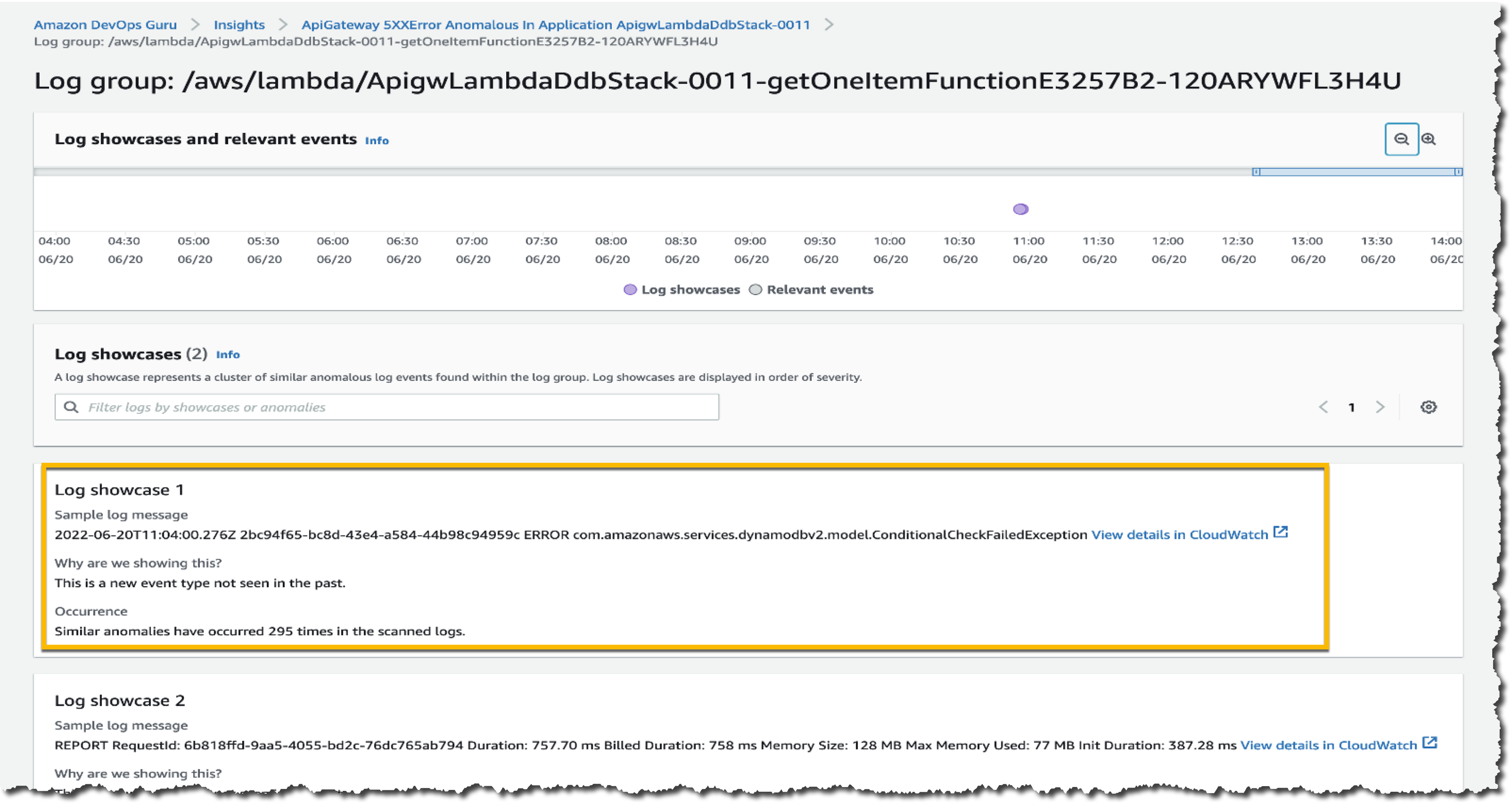
Figure 1. Data lake architecture with OpenSearch
Collect data from various sources, such as SaaS applications, edge devices, logs, streaming media, and social networks.
Validate, clean, normalize, transform, and enrich the data through a series of pre-processing steps using AWS Glue or Amazon EMR.
Place the data that is ready to be indexed in the indexing zone.
Use AWS Lambda to index the documents into OpenSearch and store them back in the data lake with a unique identifier.
Use the clean zone as the source of truth for teams to consume the data and calculate additional metrics.
Develop, train, and generate new metrics using machine learning (ML) models with Amazon SageMaker or artificial intelligence (AI) services like Amazon Comprehend.
Store the new metrics in the enriching zone along with the identifier of the OpenSearch document.
Use the identifier column from the initial indexing phase to identify the correct documents and update them in OpenSearch with the newly calculated metrics using AWS Lambda.
Use OpenSearch to search through the documents and visualize them with metrics using OpenSearch Dashboards.
Considerations
Data lake orchestration among teams
This architecture allows data teams to work independently on text documents at different stages of their lifecycles. The data engineering team manages the raw and indexing zones, who also handle data ingestion and preprocessing for indexing in OpenSearch.
The cleaned data is stored in the clean zone, where data analysts and data scientists generate insights and calculate new metrics. These metrics are stored in the enrich zone and indexed as new fields in the OpenSearch documents by the data engineering team (Figure 2).
Figure 2. Data lake orchestration among teams
Let’s explore an example. Consider a company that periodically retrieves blog site comments and performs sentiment analysis using Amazon Comprehend. In this case:
The comments are ingested into the raw zone of the data lake.
The data engineering team processes the comments and stores them in the indexing zone.
A Lambda function indexes the comments into OpenSearch, enriches the comments with the OpenSearch document ID, and saves it in the clean zone.
The data science team consumes the comments and performs sentiment analysis using Amazon Comprehend.
The sentiment analysis metrics are stored in the metrics zone of the data lake. A second Lambda function updates the comments in OpenSearch with the new metrics.
If the raw data does not require any preprocessing steps, the indexing and clean zones can be combined. You can explore this specific example, along with code implementation, in the AWS samples repository.
Schema evolution
As your data progresses through data lake stages, the schema changes and gets enriched accordingly. Continuing with our previous example, Figure 3 explains how the schema evolves.
Figure 3. Schema evolution through the data lake stages
In the raw zone, there is a raw text field received directly from the ingestion phase. It’s best practice to keep a raw version of the data as a backup, or in case the processing steps need to be repeated later.
In the indexing zone, the clean text field replaces the raw text field after being processed.
In the clean zone, we add a new ID field that is generated during indexing and identifies the OpenSearch document of the text field.
In the enrich zone, the ID field is required. Other fields with metric names are optional and represent new metrics calculated by other teams that will be added to OpenSearch.
Consumption layer with OpenSearch
In OpenSearch, data is organized into indices, which can be thought of as tables in a relational database. Each index consists of documents—similar to table rows—and multiple fields, similar to table columns. You can add documents to an index by indexing and updating them using various client APIs for popular programming languages.
Now, let’s explore how our architecture integrates with OpenSearch in the indexing and updating stage.
Indexing and updating documents using Python
The index document API operation allows you to index a document with a custom ID, or assigns one if none is provided. To speed up indexing, we can use the bulk index API to index multiple documents in one call.
We need to store the IDs back from the index operation to later identify the documents we’ll update with new metrics. Let’s explore two ways of doing this:
Use the requests library to call the REST Bulk Index API (preferred): the response returns the auto-generated IDs we need.
Use the Python Low-Level Client for OpenSearch: The IDs are not returned and need to be pre-assigned to later store them. We can use an atomic counter in Amazon DynamoDB to do so. This allows multiple Lambda functions to index documents in parallel without ID collisions.
As in Figure 4, the Lambda function:
Increases the atomic counter by the number of documents that will index into OpenSearch.
Gets the value of the counter back from the API call.
Indexes the documents using the range that goes between [current counter value, current counter value – number of documents].
Figure 4. Storing the IDs back from the bulk index operation using the Python Low-Level Client for OpenSearch
Data flow automation
As architectures evolve towards automation, the data flow between data lake stages becomes event-driven. Following our previous example, we can automate the processing steps of the data when moving from the raw to the indexing zone (Figure 5).
The same approach can be applied to the other data lake stages to achieve a fully automated architecture. Explore this implementation for an automated language use case.
Conclusion
In this blog post, we covered designing an architecture to effectively handle text data using a data lake on AWS. We explained how different data teams can work independently to extract insights from text documents at different lifecycle stages using OpenSearch as the search and analytics service.
Genomics workflows analyze data at petabyte scale. After processing is complete, data is often archived in cold storage classes. In some cases, like studies on the association of DNA variants against larger datasets, archived data is needed for further processing. This means manually initiating the restoration of each archived object and monitoring the progress. Scientists require a reliable process for on-demand archival data restoration so their workflows do not fail.
In Part 4 of this series, we look into genomics workloads processing data that is archived with Amazon Simple Storage Service (Amazon S3). We design a reliable data restoration process that informs the workflow when data is available so it can proceed. We build on top of the design pattern laid out in Parts 1-3 of this series. We use event-driven and serverless principles to provide the most cost-effective solution.
The S3 Glacier Flexible Retrieval and S3 Glacier Deep Archive provide further cost savings, with retrieval times ranging from minutes to hours. We focus on the latter in order to provide the most cost-effective solution.
You must first restore the objects before accessing them. Our genomics workflow will pause until the data restore completes. The requirements for this workflow are:
Reliable launch of the restore so our workflow doesn’t fail (due to S3 Glacier service quotas, or because not all objects were restored)
Event-driven design to mirror the event-driven nature of genomics workflows and perform the retrieval upon request
Cost-effective and easy-to-manage by using serverless services
Upfront detection of archived data when formulating the genomics workflow task, avoiding idle computational tasks that incur cost
Scalable and elastic to meet the restore needs of large, archived datasets
Solution overview
Genomics workflows take multiple input parameters to prepare the initiation, such as launch ID, data path, workflow endpoint, and workflow steps. We store this data, including workflow configurations, in an S3 bucket. An AWS Fargate task reads from the S3 bucket and prepares the workflow. It detects if the input parameters include S3 Glacier URLs.
We use Amazon Simple Queue Service (Amazon SQS) to decouple S3 Glacier index creation from object restore actions (Figure 1). This increases the reliability of our process.
Figure 1. Solution architecture for S3 Glacier object restore
An AWS Lambda function creates the index of all objects in the specified S3 bucket URLs and submits them as an SQS message.
Another Lambda function polls the SQS queue and submits the request(s) to restore the S3 Glacier objects to S3 Standard storage class.
The function writes the job ID of each S3 Glacier restore request to Amazon DynamoDB. After the restore is complete, Lambda sets the status of the workflow to READY. Only then can any computing jobs start, such as with AWS Batch.
Implementation considerations
We consider the use case of Snakemake with Tibanna, which we detailed in Part 2 of this series. This allows us to dive deeper on launch details.
Snakemake is an open-source utility for whole-genome-sequence mapping in directed acyclic graph format. Snakemake uses Snakefiles to declare workflow steps and commands. Tibanna is an open-source, AWS-native software that runs bioinformatics data pipelines. It supports Snakefile syntax, plus other workflow languages, including Common Workflow Language and Workflow Description Language (WDL).
We recommend using Amazon Genomics CLI if Tibanna is not needed for your use case, or Amazon Omics if your workflow definitions are compliant with the supported WDL and Nextflow specifications.
Formulate the restore request
The Snakemake Fargate launch container detects if the S3 objects under the requested S3 bucket URLs are stored in S3 Glacier. The Fargate launch container generates and puts a JSON binary base call (BCL) configuration file into an S3 bucket and exits successfully. This file includes the launch ID of the workflow, corresponding with the DynamoDB item key, plus the S3 URLs to restore.
Query the S3 URLs
Once the JSON BCL configuration file lands in this S3 bucket, the S3 Event NotificationPutObject event invokes a Lambda function. This function parses the configuration file and recursively queries for all S3 object URLs to restore.
Initiate the restore
The main Lambda function then submits messages to the SQS queue that contains the full list of S3 URLs that need to be restored. SQS messages also include the launch ID of the workflow. This is to ensure we can bind specific restoration jobs to specific workflow launches. If all S3 Glacier objects belong to Flexible Retrieval storage class, the Lambda function puts the URLs in a single SQS message, enabling restoration with Bulk Glacier Job Tier. The Lambda function also sets the status of the workflow to WAITING in the corresponding DynamoDB item. The WAITING state is used to notify the end user that the job is waiting on the data-restoration process and will continue once the data restoration is complete.
A secondary Lambda function polls for new messages landing in the SQS queue. This Lambda function submits the restoration request(s)—for example, as a free-of-charge Bulk retrieval—using the RestoreObject API. The function subsequently writes the S3 Glacier Job ID of each request in our DynamoDB table. This allows the main Lambda function to check if all Job IDs associated with a workflow launch ID are complete.
Update status
The status of our workflow launch will remain WAITING as long as the Glacier object restore is incomplete. The AWS CloudTrail logs of completed S3 Glacier Job IDs invoke our main Lambda function (via an Amazon EventBridge rule) to update the status of the restoration job in our DynamoDB table. With each invocation, the function checks if all Job IDs associated with a workflow launch ID are complete.
After all objects have been restored, the function updates the workflow launch with status READY. This launches the workflow with the same launch ID prior to the restore.
Conclusion
In this blog post, we demonstrated how life-science research teams can make use of their archival data for genomic studies. We designed an event-driven S3 Glacier restore process, which retrieves data upon request. We discussed how to reliably launch the restore so our workflow doesn’t fail. Also, we determined upfront if an S3 Glacier restore is needed and used the WAITING state to prevent our workflow from failing.
With this solution, life-science research teams can save money using Amazon S3 Glacier without worrying about their day-to-day work or manually administering S3 Glacier object restores.
This blog post is written by Jack Chen, Telco Solutions Architect, and Robert Belson, Developer Advocate.
AWS Wavelength embeds AWS compute and storage services within 5G networks, providing mobile edge computing infrastructure for developing, deploying, and scaling ultra-low-latency applications. AWS recently introduced support for Application Load Balancer (ALB) in AWS Wavelength zones. Although ALB addresses Layer-7 load balancing use cases, some low latency applications that get deployed in AWS Wavelength Zones rely on UDP-based protocols, such as QUIC, WebRTC, and SRT, which can’t be load-balanced by Layer-7 Load Balancers. In this post, we’ll review popular load-balancing patterns on AWS Wavelength, including a proposed architecture demonstrating how DNS-based load balancing can address customer requirements for load-balancing non-HTTP(s) traffic across multiple Amazon Elastic Compute Cloud (Amazon EC2) instances. This solution also builds a foundation for automatic scale-up and scale-down capabilities for workloads running in an AWS Wavelength Zone.
Load balancing use cases in AWS Wavelength
In the AWS Regions, customers looking to deploy highly-available edge applications often consider Amazon Elastic Load Balancing (Amazon ELB) as an approach to automatically distribute incoming application traffic across multiple targets in one or more Availability Zones (AZs). However, at the time of this publication, AWS-managed Network Load Balancer (NLB) isn’t supported in AWS Wavelength Zones and ALB is being rolled out to all AWS Wavelength Zones globally. As a result, this post will seek to document general architectural guidance for load balancing solutions on AWS Wavelength.
As one of the most prominent AWS Wavelength use cases, highly-immersive video streaming over UDP using protocols such as WebRTC at scale often require a load balancing solution to accommodate surges in traffic, either due to live events or general customer access patterns. These use cases, relying on Layer-4 traffic, can’t be load-balanced from a Layer-7 ALB. Instead, Layer-4 load balancing is needed.
To date, two infrastructure deployments involving Layer-4 load balancers are most often seen:
Amazon EC2-based deployments: Often the environment of choice for earlier-stage enterprises and ISVs, a fleet of EC2 instances will leverage a load balancer for high-throughput use cases, such as video streaming, data analytics, or Industrial IoT (IIoT) applications
Amazon EKS deployments: Customers looking to optimize performance and cost efficiency of their infrastructure can leverage containerized deployments at the edge to manage their AWS Wavelength Zone applications. In turn, external load balancers could be configured to point to exposed services via NodePort objects. Furthermore, a more popular choice might be to leverage the AWS Load Balancer Controller to provision an ALB when you create a Kubernetes Ingress.
Regardless of deployment type, the following design constraints must be considered:
Target registration: For load balancing solutions not managed by AWS, seamless solutions to load balancer target registration must be managed by the customer. As one potential solution, visit a recent HAProxyConf presentation, Practical Advice for Load Balancing at the Network Edge.
Edge Discovery: Although DNS records can be populated into Amazon Route 53 for each carrier-facing endpoint, DNS won’t deterministically route mobile clients to the most optimal mobile endpoint. When available, edge discovery services are required to most effectively route mobile clients to the lowest latency endpoint.
Cross-zone load balancing: Given the hub-and-spoke design of AWS Wavelength, customer-managed load balancers should proxy traffic only to that AWS Wavelength Zone.
Solution overview – Amazon EC2
In this solution, we’ll present a solution for a highly-available load balancing solution in a single AWS Wavelength Zone for an Amazon EC2-based deployment. In a separate post, we’ll cover the needed configurations for the AWS Load Balancer Controller in AWS Wavelength for Amazon Elastic Kubernetes Service (Amazon EKS) clusters.
The proposed solution introduces DNS-based load balancing, a technique to abstract away the complexity of intelligent load-balancing software and allow your Domain Name System (DNS) resolvers to distribute traffic (equally, or in a weighted distribution) to your set of endpoints.
Our solution leverages the weighted routing policy in Route 53 to resolve inbound DNS queries to multiple EC2 instances running within an AWS Wavelength zone. As EC2 instances for a given workload get deployed in an AWS Wavelength zone, Carrier IP addresses can be assigned to the network interfaces at launch.
Through this solution, Carrier IP addresses attached to AWS Wavelength instances are automatically added as DNS records for the customer-provided public hosted zone.
To determine how Route 53 responds to queries, given an arbitrary number of records of a public hosted zone, Route53 offers numerous routing policies:
Simple routing policy – In the event that you must route traffic to a single resource in an AWS Wavelength Zone, simple routing can be used. A single record can contain multiple IP addresses, but Route 53 returns the values in a random order to the client.
Weighted routing policy – To route traffic more deterministically using a set of proportions that you specify, this policy can be selected. For example, if you would like Carrier IP A to receive 50% of the traffic and Carrier IP B to receive 50% of the traffic, we’ll create two individual A records (one for each Carrier IP) with a weight of 50 and 50, respectively. Learn more about Route 53 routing policies by visiting the Route 53 Developer Guide.
The proposed solution leverages weighted routing policy in Route 53 DNS to route traffic to multiple EC2 instances running within an AWS Wavelength zone.
Reference architecture
The following diagram illustrates the load-balancing component of the solution, where EC2 instances in an AWS Wavelength zone are assigned Carrier IP addresses. A weighted DNS record for a host (e.g., www.example.com) is updated with Carrier IP addresses.
When a device makes a DNS query, it will be returned to one of the Carrier IP addresses associated with the given domain name. With a large number of devices, we expect a fair distribution of load across all EC2 instances in the resource pool. Given the highly ephemeral mobile edge environments, it’s likely that Carrier IPs could frequently be allocated to accommodate a workload and released shortly thereafter. However, this unpredictable behavior could yield stale DNS records, resulting in a “blackhole” – routes to endpoints that no longer exist.
Time-To-Live (TTL) is a DNS attribute that specifies the amount of time, in seconds, that you want DNS recursive resolvers to cache information about this record.
In our example, we should set to 30 seconds to force DNS resolvers to retrieve the latest records from the authoritative nameservers and minimize stale DNS responses. However, a lower TTL has a direct impact on cost, as a result of increased number of calls from recursive resolvers to Route53 to constantly retrieve the latest records.
The core components of the solution are as follows:
AWS Auto Scaling Group– a collection of EC2 instances logically grouped together for the purpose of automatic scaling.
Alongside the services above in the AWS Wavelength Zone, the following services are also leveraged in the AWS Region:
AWS Lambda – a serverless event-driven function that makes API calls to the Route 53 service to update DNS records.
Amazon EventBridge– a serverless event bus that reacts to EC2 instance lifecycle events and invokes the Lambda function to make DNS updates.
Route 53– cloud DNS service with a domain record pointing to AWS Wavelength-hosted resources.
In this post, we intentionally leave the specific load balancing software solution up to the customer. Customers can leverage various popular load balancers available on the AWS Marketplace, such as HAProxy and NGINX. To focus our solution on the auto-registration of DNS records to create functional load balancing, this solution is designed to support stateless workloads only. To support stateful workloads, sticky sessions – a process in which routes requests to the same target in a target group – must be configured by the underlying load balancer solution and are outside of the scope of what DNS can provide natively.
Automation overview
Using the aforementioned components, we can implement the following workflow automation:
Amazon CloudWatchalarm can trigger the Auto Scaling group Scale out or Scale in event by adding or removing EC2 instances. Eventbridge will detect the EC2 instance state change event and invoke the Lambda function. This function will update the DNS record in Route53 by either adding (scale out) or deleting (scale in) a weighted A record associated with the EC2 instance changing state.
Configuration of the automatic auto scaling policy is out of the scope of this post. There are many auto scaling triggers that you can consider using, based on predefined and custom metrics such as memory utilization. For the demo purposes, we will be leveraging manual auto scaling.
Amazon Virtual Private Cloud (Amazon VPC), subnets, Carrier Gateway, and Route Tables are foundational building blocks for AWS-based networking infrastructure. In our deployment, we are creating a new VPC, one subnet in an AWS Wavelength zone of your choice, a Carrier Gateway, and updating the route table for this subnet to point the default route to the Carrier Gateway.
Deployment prerequisites
The following are prerequisites to deploy the described solution in your account:
Access to an AWS Wavelength zone. If your account is not allow-listed to use AWS Wavelength zones, then opt-in to AWS Wavelength zones here.
Public DNS Hosted Zone hosted in Route 53. You must have access to a registered public domain to deploy this solution. The zone for this domain should be hosted in the same account where you plan to deploy AWS Wavelength workloads. If you don’t have a public domain, then you can register a new one. Note that there will be a service charge for the domain registration.
Amazon S3 bucket. For the Lambda function that updates DNS records in Route 53, store the source code as a .zip file in an Amazon S3 bucket.
Amazon EC2 Key pair. You can use an existing Key pair for the deployment. If you don’t have a KeyPair in the region where you plan to deploy this solution, then create one by following these instructions.
4G or 5G-connected device. Although the infrastructure can be deployed independent of the underlying connected devices, testing the connectivity will require a mobile device on one of the Wavelength partner’s networks. View the complete list of Telecommunications providers and Wavelength Zone locations to learn more.
Conclusion
In this post, we demonstrated how to implement DNS-based load balancing for workloads running in an AWS Wavelength zone. We deployed the solution that used the EventBridge Rule and the Lambda function to update DNS records hosted by Route53. If you want to learn more about AWS Wavelength, subscribe to AWS Compute Blog channel here.
Genomics workflows are high-performance computing workloads. Life-science research teams make use of various genomics workflows. With each invocation, they specify custom sets of data and processing steps, and translate them into commands. Furthermore, team members stay to monitor progress and troubleshoot errors, which can be cumbersome, non-differentiated, administrative work.
In Part 3 of this series, we describe the architecture of a workflow manager that simplifies the administration of bioinformatics data pipelines. The workflow manager dynamically generates the launch commands based on user input and keeps track of the workflow status. This workflow manager can be adapted to many scientific workloads—effectively becoming a bring-your-own-workflow-manager for each project.
In this blog post, we extend this idea to a new frontend layer in our design pattern. This layer automates command generation and monitors the invocations of a variety of workflows—becoming a workflow manager. Life-science research teams use multiple workflows for different datasets and use cases, each with different syntax and commands. The workflow manager we create removes the administrative burden of formulating workflow-specific commands and tracking their launches.
Solution overview
We allow scientists to upload their requested workflow configuration as objects in Amazon S3. We use S3 Event Notifications on PUT requests to invoke an AWS Lambda function. The function parses the uploaded S3 object and registers the new launch request as a DynamoDB item using the PutItem operation. Each item corresponds with a distinct launch request, stored as key-value pair. Item values store the:
S3 data path containing genomic datasets
Workflow endpoint
Preferred compute service (optional)
Another Lambda function monitors for change data captures in the DynamoDB Stream (Figure 1). With each PutItem operation, the Lambda function prepares a workflow invocation, which includes translating the user input into the syntax and launch commands of the respective workflow.
In the case of Snakemake (discussed in Part 2), the function creates a Snakefile that declares processing steps and commands. The function spins up an AWS Fargate task that builds the computational tasks, distributes them with AWS Batch, and monitors for completion. An AWS Step Functions state machine orchestrates job processing, for example, initiated by Tibanna.
Amazon CloudWatch provides a consolidated overview of performance metrics, like time elapsed, failed jobs, and error types. We store log data, including status updates and errors, in Amazon CloudWatch Logs. A third Lambda function parses those logs and updates the status of each workflow launch request in the corresponding DynamoDB item (Figure 1).
Figure 1. Workflow manager for genomics workflows
Implementation considerations
In this section, we describe some of our past implementation considerations.
Register new workflow requests
DynamoDB items are key-value pairs. We use launch IDs as key, and the value includes the workflow type, compute engine, S3 data path, the S3 object path to the user-defined configuration file and workflow status. Our Lambda function parses the configuration file and generates all commands plus ancillary artifacts, such as Snakefiles.
Launch workflows
Launch requests are picked by a Lambda function from the DynamoDB stream. The function has the following required parameters:
Launch ID: unique identifier of each workflow launch request
Configuration file: the Amazon S3 path to the configuration sheet with launch details (in s3://bucket/object format)
These points assume that the configuration sheet is already uploaded into an accessible location in an S3 bucket. This will issue a new Snakemake Fargate launch task. If either of the parameters is not provided or access fails, the workflow manager returns MissingRequiredParametersError.
Log workflow launches
Logs are written to CloudWatch Logs automatically. We write the location of the CloudWatch log group and log stream into the DynamoDB table. To send logs to Amazon CloudWatch, specify the awslogs driver in the Fargate task definition settings in your provisioning template.
Our Lambda function writes Fargate task launch logs from CloudWatch Logs to our DynamoDB table. For example, OutOfMemoryError can occur if the process utilizes more memory than the container is allocated.
AWS Batch job state logs are written to the following log group in CloudWatch Logs: /aws/batch/job. Our Lambda function writes status updates to the DynamoDB table. AWS Batch jobs may encounter errors, such as being stuck in RUNNABLE state.
Manage state transitions
We manage the status of each job in DynamoDB. Whenever a Fargate task changes state, it is picked up by a CloudWatch rule that references the Fargate compute cluster. This CloudWatch rule invokes a notifier Lambda function that updates the workflow status in DynamoDB.
Conclusion
In this blog post, we demonstrated how life-science research teams can simplify genomic analysis across an array of workflows. These workflows usually have their own command syntax and workflow management system, such as Snakemake. The presented workflow manager removes the administrative burden of preparing and formulating workflow launches, increasing reliability.
The pattern is broadly reusable with any scientific workflow and related high-performance computing systems. The workflow manager provides persistence to enable historical analysis and comparison, which enables us to automatically benchmark workflow launches for cost and performance.
Many organizations require durable automated code delivery for their applications. They leverage multi-account continuous integration/continuous deployment (CI/CD) pipelines to deploy code and run automated tests in multiple environments before deploying to Production. In cases where the testing strategy is release specific, you must update the pipeline before every release. Traditional pipeline stages are predefined and static in nature, and once the pipeline stages are defined it’s hard to update them. In this post, we present a configuration driven dynamic CI/CD solution per repository. The pipeline state is maintained and governed by configurations stored in Amazon DynamoDB. This gives you the advantage of automatically customizing the pipeline for every release based on the testing requirements.
The following diagram illustrates the solution architecture:
Figure 1: Architecture Diagram
Users insert/update/delete entry in the DynamoDB table.
The Step Function Trigger Lambda is invoked on all modifications.
The Step Function Trigger Lambda evaluates the incoming event and does the following:
On insert and update, triggers the Step Function.
On delete, finds the appropriate CloudFormation stack and deletes it.
Steps in the Step Function are as follows:
Collect Information (Pass State) – Filters the relevant information from the event, such as repositoryName and referenceName.
Get Mapping Information (Backed by CodeCommit event filter Lambda) – Retrieves the mapping information from the Pipeline config stored in the DynamoDB.
Deployment Configuration Exist? (Choice State) – If the StatusCode == 200, then the DynamoDB entry is found, and Initiate CloudFormation Stack step is invoked, or else StepFunction exits with Successful.
Initiate CloudFormation Stack (Backed by stack create Lambda) – Constructs the CloudFormation parameters and creates/updates the dynamic pipeline based on the configuration stored in the DynamoDB via CloudFormation.
Code deliverables
The code deliverables include the following:
AWS CDK app – The AWS CDK app contains the code for all the Lambdas, Step Functions, and CloudFormation templates.
sample-application-repo – This directory contains the sample application repository used for deployment.
automated-tests-repo– This directory contains the sample automated tests repository for testing the sample repo.
Follow the README to deploy the solution to your main CI/CD account. Upon successful deployment, the following resources should be created in the CI/CD account:
A DynamoDB table
Step Function
Lambda Functions
Navigate to the Amazon Simple Storage Service (Amazon S3) console in your main CI/CD account and search for a bucket with the name: cloudformation-template-bucket-<AWS_ACCOUNT_ID>. You should see two CloudFormation templates (templates/codepipeline.yaml and templates/childaccount.yaml) uploaded to this bucket.
Run the childaccount.yaml in every target CI/CD account (Alpha, Beta, Gamma, and Prod) by going to the CloudFormation Console. Provide the main CI/CD account number as the “CentralAwsAccountId” parameter, and execute.
Upon successful creation of Stack, two roles will be created in the Child Accounts:
ChildAccountFormationRole
ChildAccountDeployerRole
Pipeline configuration
Make an entry into devops-pipeline-table-info for the Repository name and branch combination. A sample entry can be found in sample-entry.json.
The pipeline is highly configurable, and everything can be configured through the DynamoDB entry.
The following are the top-level keys:
RepoName: Name of the repository for which AWS CodePipeline is configured. RepoTag: Name of the branch used in CodePipeline. BuildImage: Build image used for application AWS CodeBuild project. BuildSpecFile: Buildspec file used in the application CodeBuild project. DeploymentConfigurations: This key holds the deployment configurations for the pipeline. Under this key are the environment specific configurations. In our case, we’ve named our environments Alpha, Beta, Gamma, and Prod. You can configure to any name you like, but make sure that the entries in json are the same as in the codepipeline.yaml CloudFormation template. This is because there is a 1:1 mapping between them. Sub-level keys under DeploymentConfigurations are as follows:
EnvironmentName. This is the top-level key for environment specific configuration. In our case, it’s Alpha, Beta, Gamma, and Prod. Sub level keys under this are:
<Env>AwsAccountId: AWS account ID of the target environment.
Deploy<Env>: A key specifying whether or not the artifact should be deployed to this environment. Based on its value, the CodePipeline will have a deployment stage to this environment.
ManualApproval<Env>: Key representing whether or not manual approval is required before deployment. Enter your email or set to false.
Tests: Once again, this is a top-level key with sub-level keys. This key holds the test related information to be run on specific environments. Each test based on whether or not it will be run will add an additional step to the CodePipeline. The tests’ related information is also configurable with the ability to specify the test repository, branch name, buildspec file, and build image for testing the CodeBuild project.
Execute
Make an entry into the devops-pipeline-table-info DynamoDB table in the main CI/CD account. A sample entry can be found in sample-entry.json. Make sure to replace the configuration values with appropriate values for your environment. An explanation of the values can be found in the Pipeline Configuration section above.
After the entry is made in the DynamoDB table, you should see a CloudFormation stack being created. This CloudFormation stack will deploy the CodePipeline in the main CI/CD account by reading and using the entry in the DynamoDB table.
Customize the solution for different combinations such as deploying to an environment while skipping for others by updating the pipeline configurations stored in the devops-pipeline-table-info DynamoDB table. The following is the pipeline configured for the sample-application repository’s main branch.
Figure 2: Dynamic Multi-Account CI/CD Pipeline
Clean up your dynamic multi-account CI/CD solution and related resources
To avoid ongoing charges for the resources that you created following this post, you should delete the following:
The pipeline configuration stored in the DynamoDB
The CloudFormation stacks deployed in the target CI/CD accounts
The AWS CDK app deployed in the main CI/CD account
Empty and delete the retained S3 buckets.
Conclusion
This configuration-driven CI/CD solution provides the ability to dynamically create and configure your pipelines in DynamoDB. IDEMIA, a global leader in identity technologies, adopted this approach for deploying their microservices based application across environments. This solution created by AWS Professional Services allowed them to dynamically create and configure their pipelines per repository per release. As Kunal Bajaj, Tech Lead of IDEMIA, states, “We worked with AWS pro-serve team to create a dynamic CI/CD solution using lambdas, step functions, SQS, and other native AWS services to conduct cross-account deployments to our different environments while providing us the flexibility to add tests and approvals as needed by the business.”
Amazon DynamoDB is ideal for applications that need a flexible NoSQL database with low read and write latencies and the ability to scale storage and throughput up or down as needed without code changes or downtime. You can use DynamoDB for use cases including mobile apps, gaming, digital ad serving, live voting, audience interaction for live events, sensor networks, log ingestion, access control for web-based content, metadata storage for Amazon S3 objects, e-commerce shopping carts, and web session management.
What if you have the need to allow other AWS accounts to query your DynamoDB table? What if other accounts need to join data on your DynamoDB table with their data stored in data sources like Amazon CloudWatch, Amazon DocumentDB, Amazon Redshift, Amazon OpenSearch, MySQL, PostgreSQL connected with Athena data source connectors, and Amazon S3?
Amazon Athena cross-account federated query enables you to run SQL queries across data stored in relational, non-relational, object, and custom data sources where data source and its connector are in different AWS accounts from the user querying the data. There are no new charges for querying connectors in another account, but Athena’s standard rates for data scanned, Lambda usage, and other services apply.
This post will demonstrate Athena in an AWS account accessing a DynamoDB table of another AWS account by using the Athena cross-account federated query. It also explains deploying Amazon Athena DynamoDB connector using AWS Serverless Application Repository and setting up Athena cross-account federation between two accounts for the Demo.
Walkthrough
The solution has the following steps to demonstrate Athena cross-account federated query:
Set up Athena federation – To deploy a Lambda function for the data source connector and connect it to a data source.
Set up Athena cross-account federation – To set up IAM permissions for Athena cross-account federation.
Test Athena cross-account federated query – To show a demo of how an AWS account can share its DynamoDB table as an Athena data source with another AWS account.
Prerequisites
For this walkthrough, you should have the following prerequisites:
A data source connector is a piece of code that can translate between your target data source and Athena. Athena uses data source connectors that run on AWS Lambda to run federated queries. You can think of a connector as an extension of Athena’s query engine.
Connectors use Apache Arrow as the format for returning data requested in a query, which enables connectors to be implemented in languages such as C, C++, Java, Python, and Rust.
Athena uses data source connectors that run on AWS Lambda to run federated queries. Since connectors are processed in Lambda, they can be used to access data from any data source on the cloud or on premises that is accessible from Lambda
To use a connector in your Athena queries, deploy it to your account using one of the following ways:
After you deploy data source connectors, the connector is associated with a catalog that you can specify in SQL queries. You can combine SQL statements from multiple catalogs and span multiple data sources with a single query. When a query is submitted against a data source, Athena invokes the corresponding connector to identify parts of the tables that need to be read, manages parallelism, and pushes down filter predicates. Based on the user submitting the query, connectors can provide or restrict access to specific data elements.
Architecture
AWS Account-A has a DynamoDB table called Music.
Account-A has an Athena data source connector to federate into DynamoDB.
AWS Account-B has Analysts who need to query the DynamoDB table.
Account-A is sharing the Athena data source with Account-B by using Athena cross-account federated query.
The following figure shows Amazon Athena cross-account federation for Account-B to access DynamoDB in Account-A.
To demonstrate the Athena cross-account federation, create a sample DynamoDB table called music in Account-A. Follow the instructions at Getting started with DynamoDB to create the table Music and load thesample data.
Set up Athena federation
Preparing to create federated queries is a two-part process: deploying a Lambda function for the data source connector and connecting the Lambda function to a data source. For more details, see Enabling cross-account federated queries.
Deploy AthenaDynamoDBConnector using AWS Serverless Application Repository
Sign in as an administrator to AWS Account-A.
Open the Serverless Application Repository.
In the navigation pane, choose Available applications.
Select the option Show apps that create custom IAM roles or resource policies.
In the search box, type the name of the connector AthenaDynamoDBConnector.
Choosing a connector opens the Lambda function’s Application details page in the AWS Lambda console.
On the right side of the details page, for Application settings, fill in the required information.
Application name – Name of AWS CloudFormation Stack to deploy the connector: AthenaDynamoDBConnector.
AthenaCatalogName – It is the catalog name to create in Athena. It is also the name of the Lambda function. Give it in lowercase: acct1dynamodb.
SpillBucket – Specify an existing S3 bucket (spill-bucket) in your account to receive data from any large response payloads that exceed Lambda function response size limits.
Select I acknowledge that this app creates custom IAM roles and resource policies. For more information, choose the Info link.
At the bottom right of the Application settings section, choose Deploy.
Serverless Application Repository will create an AWS CloudFormation stack to deploy the connector.
When the deployment is complete, you will see the Lambda function in the Resources section of the AWS CloudFormation stack. Note down the Lambda function name.
Connect Athena to the data source
Go to Athena console in Account-A.
Choose Data sources. Click Create Data source.
In Choose data source, search for Amazon DynamoDB and select it.
In Data source details, give a Data source nameacct1dynamodb
For Lambda function in the Connection details section, choose the name of the function acct1dynamodb from the dropdown.
On the Review and create page, review the data source details, and then choose Create data source.
You will see the data source acctdynamodb in the Data sources.
Go to Query editor. Choose the Data Source acct1dynamodb from the dropdown.
You will see all the tables in the shared data source.
Run the following SQL in Athena Query editor
SELECT songtitle, albumtitle, cast(awards as int) as awards
FROM "acct1dynamodb"."default"."music"
WHERE artist = 'Acme Band'
limit 2;
Verify Athena federation works.
Set up Athena cross-account federation
In Account-A: Set up IAM permissions for cross-account
Sign in as an administrator to Account-A.
On the S3 spill bucket (of the Lambda function), grant GetObject and ListBucket permissions to the IAM user analyst of Account-B.
Note: Replace Account-B-id with your actual AWS cross-account id to which you want to share the DynamoDB table. Replace spill-bucket with your actual S3 bucket in Account-A.
Grant InvokeFunction on Lambda function acct1dynamodb to IAM user analyst of Account-B.
Note: Replace Account-A-id with your actual AWS account id where you have the DynamoDB table. Replace Account-B-id with your actual AWS cross-account id to which you want to share the DynamoDB table.
After the permissions are in place, you share a data connector in your account (Account-A) with another account (Account-B). Account-A retains full control and ownership of the connector. When Account-A makes configuration changes to the connector, the updated configuration applies to the shared connector in Account-B.
Sign in as an administrator to Account-A.
On Athena, go to Data sources, choose data source acct1dynamodb you want to share. Go to the Share option in the top right corner.
For Account ID, enter the Account-B-id to share your data source with Account-B and click Share.
Test Athena cross-account federated query: Access the shared data source from Account-B
Sign in as IAM user analyst to Account-B.
In Athena, go to Data sources. You will see the data source acct1dynamodb.
Go to Query editor. Choose the Data Source acct1dynamodb from the dropdown.
You will see all the tables in the shared data source.
Run the following SQL in Athena Query editor
SELECT songtitle, albumtitle, cast(awards as int) as awards
FROM "acct1dynamodb"."default"."music"
WHERE artist = 'Acme Band'
limit 2;
Athena cross-account federated has worked! This validates that user analyst in Account-B can see the data of the DynamoDB table of Account-A.
Clean up
To avoid incurring future charges, delete the following resources that were provisioned for this demo:
S3 spill bucket used in AWS Lambda
Lambda function used for the data source connector
Sample DynamoDB table
Conclusion
In this post, we saw how you can access a cross-account DynamoDB table using Athena Federated Query to query the data in place. You can execute a single SQL query to join this data across data sources like Amazon CloudWatch, Amazon DocumentDB, Amazon Redshift, Amazon OpenSearch, MySQL, PostgreSQL, Oracle, SQL Server, HBase, Redis, BigQuery, Snowflake, Teradata with Athena data source connectors and Amazon S3.
About the author
Satya Adimula is a Senior Data Architect at AWS based in Boston. With extensive experience in data and analytics, Satya helps organizations derive their business insights from the data at scale.
SOCAR is the leading Korean mobility company with strong competitiveness in car-sharing. SOCAR has become a comprehensive mobility platform in collaboration with Nine2One, an e-bike sharing service, and Modu Company, an online parking platform. Backed by advanced technology and data, SOCAR solves mobility-related social problems, such as parking difficulties and traffic congestion, and changes the car ownership-oriented mobility habits in Korea.
SOCAR is building a new fleet management system to manage the many actions and processes that must occur in order for fleet vehicles to run on time, within budget, and at maximum efficiency. To achieve this, SOCAR is looking to build a highly scalable data platform using AWS services to collect, process, store, and analyze internet of things (IoT) streaming data from various vehicle devices and historical operational data.
This in-car device data, combined with operational data such as car details and reservation details, will provide a foundation for analytics use cases. For example, SOCAR will be able to notify customers if they have forgotten to turn their headlights off or to schedule a service if a battery is running low. Unfortunately, the previous architecture didn’t enable the enrichment of IoT data with operational data and couldn’t support streaming analytics use cases.
AWS Data Lab offers accelerated, joint-engineering engagements between customers and AWS technical resources to create tangible deliverables that accelerate data and analytics modernization initiatives. The Build Lab is a 2–5-day intensive build with a technical customer team.
In this post, we share how SOCAR engaged the Data Lab program to assist them in building a prototype solution to overcome these challenges, and to build the basis for accelerating their data project.
Use case 1: Streaming data analytics and real-time control
SOCAR wanted to utilize IoT data for a new business initiative. A fleet management system, where data comes from IoT devices in the vehicles, is a key input to drive business decisions and derive insights. This data is captured by AWS IoT and sent to Amazon Managed Streaming for Apache Kafka (Amazon MSK). By joining the IoT data to other operational datasets, including reservations, car information, device information, and others, the solution can support a number of functions across SOCAR’s business.
An example of real-time monitoring is when a customer turns off the car engine and closes the car door, but the headlights are still on. By using IoT data related to the car light, door, and engine, a notification is sent to the customer to inform them that the car headlights should be turned off.
Although this real-time control is important, they also want to collect historical data—both raw and curated data—in Amazon Simple Storage Service (Amazon S3) to support historical analytics and visualizations by using Amazon QuickSight.
Use case 2: Detect table schema change
The first challenge SOCAR faced was existing batch ingestion pipelines that were prone to breaking when schema changes occurred in the source systems. Additionally, these pipelines didn’t deliver data in a way that was easy for business analysts to consume. In order to meet the future data volumes and business requirements, they needed a pattern for the automated monitoring of batch pipelines with notification of schema changes and the ability to continue processing.
The second challenge was related to the complexity of the JSON files being ingested. The existing batch pipelines weren’t flattening the five-level nested structure, which made it difficult for business users and analysts to gain business insights without any effort on their end.
Overview of solution
In this solution, we followed the serverless data architecture to establish a data platform for SOCAR. This serverless architecture allowed SOCAR to run data pipelines continuously and scale automatically with no setup cost and without managing servers.
AWS Glue is used for both the streaming and batch data pipelines. Amazon Kinesis Data Analytics is used to deliver streaming data with subsecond latencies. In terms of storage, data is stored in Amazon S3 for historical data analysis, auditing, and backup. However, when frequent reading of the latest snapshot data is required by multiple users and applications concurrently, the data is stored and read from Amazon DynamoDB tables. DynamoDB is a key-value and document database that can support tables of virtually any size with horizontal scaling.
Let’s discuss the components of the solution in detail before walking through the steps of the entire data flow.
Component 1: Processing IoT streaming data with business data
The first data pipeline (see the following diagram) processes IoT streaming data with business data from an Amazon Aurora MySQL-Compatible Edition database.
Whenever a transaction occurs in two tables in the Aurora MySQL database, this transaction is captured as data and then loaded into two MSK topics via AWS Database Management (AWS DMS) tasks. One topic conveys the car information table, and the other topic is for the device information table. This data is loaded into a single DynamoDB table that contains all the attributes (or columns) that exist in the two tables in the Aurora MySQL database, along with a primary key. This single DynamoDB table contains the latest snapshot data from the two DB tables, and is important because it contains the latest information of all the cars and devices for the lookup against the streaming IoT data. If the lookup were done on the database directly with the streaming data, it would impact the production database performance.
When the snapshot is available in DynamoDB, an AWS Glue streaming job runs continuously to collect the IoT data and join it with the latest snapshot data in the DynamoDB table to produce the up-to-date output, which is written into another DynamoDB table.
The up-to-date data in DynamoDB is used for real-time monitoring and control that SOCAR’s Data Analytics team performs for safety maintenance and fleet management. This data is ultimately consumed by a number of apps to perform various business activities, including route optimization, real-time monitoring for oil consumption and temperature, and to identify a driver’s driving pattern, tire wear and defect detection, and real-time car crash notifications.
Component 2: Processing IoT data and visualizing the data in dashboards
The second data pipeline (see the following diagram) batch processes the IoT data and visualizes it in QuickSight dashboards.
There are two data sources. The first is the Aurora MySQL database. The two database tables are exported into Amazon S3 from the Aurora MySQL cluster and registered in the AWS Glue Data Catalog as tables. The second data source is Amazon MSK, which receives streaming data from AWS IoT Core. This requires you to create a secure AWS Glue connection for an Apache Kafka data stream. SOCAR’s MSK cluster requires SASL_SSL as a security protocol (for more information, refer to Authentication and authorization for Apache Kafka APIs). To create an MSK connection in AWS Glue and set up connectivity, we use the following CLI command:
The third data pipeline processes the streaming IoT data in millisecond latency from Amazon MSK to produce the output in DynamoDB, and sends a notification in real time if any records are identified as an outlier based on business rules.
AWS IoT Core provides integrations with Amazon MSK to set up real-time streaming data pipelines. To do so, complete the following steps:
On the AWS IoT Core console, choose Act in the navigation pane.
Choose Rules, and create a new rule.
For Actions, choose Add action and choose Kafka.
Choose the VPC destination if required.
Specify the Kafka topic.
Specify the TLS bootstrap servers of your Amazon MSK cluster.
You can view the bootstrap server URLs in the client information of your MSK cluster details. The AWS IoT rule was created with the Kafka topic as an action to provide data from AWS IoT Core to Kafka topics.
SOCAR used Amazon Kinesis Data Analytics Studio to analyze streaming data in real time and build stream-processing applications using standard SQL and Python. We created one table from the Kafka topic using the following code:
CREATE TABLE table_name (
column_name1 VARCHAR,
column_name2 VARCHAR(100),
column_name3 VARCHAR,
column_name4 as TO_TIMESTAMP (`time_column`, 'EEE MMM dd HH:mm:ss z yyyy'),
 WATERMARK FOR column AS column -INTERVAL '5' SECOND
)
PARTITIONED BY (column_name5)
WITH (
'connector'= 'kafka',
'topic' = 'topic_name',
'properties.bootstrap.servers' = '<bootstrap servers shown in the MSK client info dialog>',
'format' = 'json',
'properties.group.id' = 'testGroup1',
'scan.startup.mode'= 'earliest-offset'
);
Then we applied a query with business logic to identify a particular set of records that need to be alerted. When this data is loaded back into another Kafka topic, AWS Lambda functions trigger the downstream action: either load the data into a DynamoDB table or send an email notification.
Component 4: Flattening the nested structure JSON and monitoring schema changes
The final data pipeline (see the following diagram) processes complex, semi-structured, and nested JSON files.
This step uses an AWS Glue DynamicFrame to flatten the nested structure and then land the output in Amazon S3. After the data is loaded, it’s scanned by an AWS Glue crawler to update the Data Catalog table and detect any changes in the schema.
Data flow: Putting it all together
The following diagram illustrates our complete data flow with each component.
Let’s walk through the steps of each pipeline.
The first data pipeline (in red) processes the IoT streaming data with the Aurora MySQL business data:
AWS DMS is used for ongoing replication to continuously apply source changes to the target with minimal latency. The source includes two tables in the Aurora MySQL database tables (carinfo and deviceinfo), and each is linked to two MSK topics via AWS DMS tasks.
There is a single DynamoDB table with columns that exist from the carinfo table and the deviceinfo table of the Aurora MySQL database. This table consists of all the data from two tables and stores the latest data by performing an upsert operation.
An AWS Glue job continuously receives the IoT data and joins it with data in the DynamoDB table to produce the output into another DynamoDB target table.
This target table contains the final data, which includes all the device and car status information from the IoT devices as well as metadata from the Aurora MySQL table.
The second data pipeline (in green) batch processes IoT data to use in dashboards and for visualization:
The car and reservation data (in two DB tables) is exported via a SQL command from the Aurora MySQL database with the output data available in an S3 bucket. The folders that contain data are registered as an S3 location for the AWS Glue crawler and become available via the AWS Glue Data Catalog.
The MSK input topic continuously receives data from AWS IoT. Each car has a number of IoT devices, and each device captures data and sends it to an MSK input topic. The Amazon MSK S3 sink connector is configured to export data from Kafka topics to Amazon S3 in JSON formats. In addition, the S3 connector exports data by guaranteeing exactly-once delivery semantics to consumers of the S3 objects it produces.
The AWS Glue job runs in a daily batch to load the historical IoT data into Amazon S3 and into two tables (refer to step 1) to produce the output data in an Enriched folder in Amazon S3.
Amazon Athena is used to query data from Amazon S3 and make it available as a dataset in QuickSight for visualizing historical data.
The third data pipeline (in blue) processes streaming IoT data from Amazon MSK with millisecond latency to produce the output in DynamoDB and send a notification:
An Amazon Kinesis Data Analytics Studio notebook powered by Apache Zeppelin and Apache Flink is used to build and deploy its output as a Kinesis Data Analytics application. This application loads data from Amazon MSK in real time, and users can apply business logic to select particular events coming from the IoT real-time data, for example, the car engine is off and the doors are closed, but the headlights are still on. The particular event that users want to capture can be sent to another MSK topic (Outlier) via the Kinesis Data Analytics application.
Amazon MSK triggers a Lambda function, so whenever a topic receives data, a Lambda function runs to send an email notification to users that are subscribed to an Amazon Simple Notification Service (Amazon SNS) topic. An email is published using an SNS notification.
The Kinesis Data Analytics application loads data from AWS IoT, applies business logic, and then loads it into another MSK topic (output). Amazon MSK triggers a Lambda function when data is received, which loads data into a DynamoDB Append table.
Amazon Kinesis Data Analytics Studio is used to run SQL commands for ad hoc interactive analysis on streaming data.
The final data pipeline (in yellow) processes complex, semi-structured, and nested JSON files, and sends a notification when a schema evolves.
An AWS Glue job runs and reads the JSON data from Amazon S3 (as a source), applies logic to flatten the nested schema using a DynamicFrame, and pivots out array columns from the flattened frame.
The output is stored in Amazon S3 and is automatically registered to the AWS Glue Data Catalog table.
Whenever there is a new attribute or change in the JSON input data at any level in the nested structure, the new attribute and change are captured in Amazon EventBridge as an event from the AWS Glue Data Catalog. An email notification is published using Amazon SNS.
Conclusion
As a result of the four-day Build Lab, the SOCAR team left with a working prototype that is custom fit to their needs, gaining a clear path to production. The Data Lab allowed the SOCAR team to build a new streaming data pipeline, enrich IoT data with operational data, and enhance the existing data pipeline to process complex nested JSON data. This establishes a baseline architecture to support the new fleet management system beyond the car-sharing business.
About the Authors
DoYeun Kim is the Head of Data Engineering at SOCAR. He is a passionate software engineering professional with 19+ years experience. He leads a team of 10+ engineers who are responsible for the data platform, data warehouse and MLOps engineering, as well as building in-house data products.
SangSu Park is a Lead Data Architect in SOCAR’s cloud DB team. His passion is to keep learning, embrace challenges, and strive for mutual growth through communication. He loves to travel in search of new cities and places.
YoungMin Park is a Lead Architect in SOCAR’s cloud infrastructure team. His philosophy in life is-whatever it may be-to challenge, fail, learn, and share such experiences to build a better tomorrow for the world. He enjoys building expertise in various fields and basketball.
Younggu Yun is a Senior Data Lab Architect at AWS. He works with customers around the APAC region to help them achieve business goals and solve technical problems by providing prescriptive architectural guidance, sharing best practices, and building innovative solutions together. In his free time, his son and he are obsessed with Lego blocks to build creative models.
Vicky Falconer leads the AWS Data Lab program across APAC, offering accelerated joint engineering engagements between teams of customer builders and AWS technical resources to create tangible deliverables that accelerate data analytics modernization and machine learning initiatives.
In the next few years, companies will build over 500 million new applications, more than has been developed in the previous 40 years combined (see IDC article). API operations enable innovation. They are the “front door” to applications and microservices, and an integral layer in the application stack. In recent years, GraphQL has emerged as a modern API approach. With GraphQL, companies can improve the performance of their applications and the speed in which development teams can build applications. In this post, we will discuss how GraphQL works and how integrating it with AWS services can help you build modern applications. We will explore the options for running GraphQL on AWS.
How GraphQL works
Imagine you have an API frontend implemented with GraphQL for your ecommerce application. As shown in Figure 1, there are different services in your ecommerce system backend that are accessible via different technologies. For example, user profile data is stored in a highly scalable NoSQL table. Orders are accessed through a REST API. The current inventory stock is checked through an AWS Lambda function. And the pricing information is in an SQL database.
Figure 1. How GraphQL works
Without using GraphQL, client applications must make multiple separate calls to each one of these services. Because each service is exposed through different API endpoints, the complexity of accessing data from the client side increases significantly. In order to get the data, you have to make multiple calls. In some cases, you might over fetch data as the data source would send you an entire payload including data you might not need. In some other circumstances, you might under fetch data as a single data source would not have all your required data.
A GraphQL API combines the data from all these different services into a single payload that the client defines based on its needs. For example, a smartphone has a smaller screen than a desktop application. A smartphone application might require less data. The data is retrieved from multiple data sources automatically. The client just sees a single constructed payload. This payload might be receiving user profile data from Amazon DynamoDB, or order details from Amazon API Gateway. Or it could involve the injection of specific fields with inventory availability and price data from AWS Lambda and Amazon Aurora.
When modernizing frontend APIs with GraphQL, you can build applications faster because your frontend developers don’t need to wait for backend service teams to create new APIs for integration. GraphQL simplifies data access by interacting with data from multiple data sources using a single API. This reduces the number of API requests and network traffic, which results in improved application performance. Furthermore, GraphQL subscriptions enable two-way communication between the backend and client. It supports publishing updates to data in real time to subscribed clients. You can create engaging applications in real time with use cases such as updating sports scores, bidding statuses, and more.
Options for running GraphQL on AWS
There are two main options for running GraphQL implementation on AWS, fully managed on AWS using AWS AppSync, and self-managed GraphQL.
I. Fully managed using AWS AppSync
The most straightforward way to run GraphQL is by using AWS AppSync, a fully managed service. AWS AppSync handles the heavy lifting of securely connecting to data sources, such as Amazon DynamoDB, and to develop GraphQL APIs. You can write business logic against these data sources by choosing code templates that implement common GraphQL API patterns. Your APIs can also interact with other AWS AppSync functionality such as caching, to improve performance. Use subscriptions to support real-time updates, and client-side data stores to keep offline devices in sync. AWS AppSync will scale automatically to support varied API request loads. You can find more details from the AWS AppSync features page.
Figure 2. AWS AppSync in an ecommerce system implementation
Let’s take a closer look at this GraphQL implementation with AWS AppSync in an ecommerce system. In Figure 2, a schema is created to define types and capabilities of the desired GraphQL API. You can tie the schema to a Resolver function. The schema can either be created to mirror existing data sources, or AWS AppSync can create tables automatically based the schema definition. You can also use GraphQL features for data discovery without viewing the backend data sources.
After a schema definition is established, an AWS AppSync client can be configured with an operation request, such as a query operation. The client submits the operation request to GraphQL Proxy along with an identity context and credentials. The GraphQL Proxy passes this request to the Resolver, which maps and initiates the request payload against pre-configured AWS data services. These can be an Amazon DynamoDB table for user profile, an AWS Lambda function for inventory service, and more. The Resolver initiates calls to one or all of these services within a single API call. This minimizes CPU cycles and network bandwidth needs. The Resolver then returns the response to the client. Additionally, the client application can change data requirements in code on demand. The AWS AppSync GraphQL API will dynamically map requests for data accordingly, enabling faster prototyping and development.
II. Self-Managed GraphQL
If you want the flexibility of selecting a particular open-source project, you may choose to run your own GraphQL API layer. Apollo, graphql-ruby, Juniper, gqlgen, and Lacinia are some popular GraphQL implementations. You can leverage AWS Lambda or container services such as Amazon Elastic Container Service (ECS) and Amazon Elastic Kubernetes Services (EKS) to run GraphQL open-source implementations. This gives you the ability to fine-tune the operational characteristics of your API.
When running a GraphQL API layer on AWS Lambda, you can take advantage of the serverless benefits of automatic scaling, paying only for what you use, and not having to manage your servers. You can create a private GraphQL API using Amazon ECS, EKS, or AWS Lambda, which can only be accessed from your Amazon Virtual Private Cloud (VPC). With Apollo GraphQL open-source implementation, you can create a Federated GraphQL that allows you to combine GraphQL APIs from multiple microservices into a single API, illustrated in Figure 3. The Apollo GraphQL Federation with AWS AppSync post shows a concrete example of how to integrate an AWS AppSync API with an Apollo Federation gateway. It uses specification-compliant queries and directives.
Figure 3. Apollo GraphQL implementation on AWS Lambda
When choosing self-managed GraphQL implementation, you have to spend time writing non-business logic code to connect data sources. You must implement authorization, authentication, and integrate other common functionalities. This can be caches to improve performance, subscriptions to support real-time updates, and client-side data stores to keep offline devices in sync. Because of these responsibilities, you have less time to focus on the business logic of application.
Similarly, backend development teams and API operators of an open-source GraphQL implementation must provision and maintain their own GraphQL servers. Remember that even with a serverless model, API developers and operators are still responsible for monitoring, performance tuning, and troubleshooting the API platform service.
Conclusion
Modernizing APIs with GraphQL gives your frontend application the ability to fetch just the data that’s needed from multiple data sources with an API call. You can build modern mobile and web applications faster, because GraphQL simplifies API management. You have flexibility to run an open-source GraphQL implementation most closely aligned with your needs on AWS Lambda, Amazon ECS, and Amazon EKS. With AWS AppSync, you can set up GraphQL quickly and increase your development velocity by reducing the amount of non-business API logic code.
This post is co-written with Dr. Quan Hoang Nguyen, CTO at Fantom Foundation.
Here at Fantom Foundation (Fantom), we have developed a high performance, highly scalable, and secure smart contract platform. It’s designed to overcome limitations of the previous generation of blockchain platforms. The Fantom platform is permissionless, decentralized, and open source. The majority of decentralized applications (dApps) hosted on the Fantom platform lack an analytics page that provides information to the users. Therefore, we would like to build a data platform that supports a web interface that will be made public. This will allow users to search for a smart contract address. The application then displays key metrics for that smart contract. Such an analytics platform can give insights and trends for applications deployed on the platform to the users, while the developers can continue to focus on improving their dApps.
AWS Data Lab offers accelerated, joint-engineering engagements between customers and AWS technical resources to create tangible deliverables that accelerate data and analytics modernization initiatives. Data Lab has three offerings: the Build Lab, the Design Lab, and a Resident Architect. The Build Lab is a 2–5 day intensive build with a technical customer team. The Design Lab is a half-day to 2-day engagement for customers who need a real-world architecture recommendation based on AWS expertise, but aren’t yet ready to build. Both engagements are hosted either online or at an in-person AWS Data Lab hub. The Resident Architect provides AWS customers with technical and strategic guidance in refining, implementing, and accelerating their data strategy and solutions over a 6-month engagement.
In this post, we share the experience of our engagement with AWS Data Lab to accelerate the initiative of developing a data pipeline from an idea to a solution. Over 4 weeks, we conducted technical design sessions, reviewed architecture options, and built the proof of concept data pipeline.
Use case review
The process started with us engaging with our AWS Account team to submit a nomination for the data lab. This followed by a call with the AWS Data Lab team to assess the suitability of requirements against the program. After the Build Lab was scheduled, an AWS Data Lab Architect engaged with us to conduct a series of pre-lab calls to finalize the scope, architecture, goals, and success criteria for the lab. The scope was to design a data pipeline that would ingest and store historical and real-time on-chain transactions data, and build a data pipeline to generate key metrics. Once ingested, data should be transformed, stored, and exposed via REST-based APIs and consumed by a web UI to display key metrics. For this Build Lab, we choose to ingest data for Spooky, which is a decentralized exchange (DEX) deployed on the Fantom platform and had the largest Total Value Locked (TVL) at that time. Key metrics such number of wallets that have interacted with the dApp over time, number of tokens and their value exchanged for the dApp over time, and number of transactions for the dApp over time were selected to visualize through a web-based UI.
We explored several architecture options and picked one for the lab that aligned closely with our end goal. The total historical data for the selected smart contract was approximately 1 GB since deployment of dApp on the Fantom platform. We used FTMScan, which allows us to explore and search on the Fantom platform for transactions, to estimate the rate of transfer transactions to be approximately three to four per minute. This allowed us to design an architecture for the lab that can handle this data ingestion rate. We agreed to use an existing application known as the data producer that was developed internally by the Fantom team to ingest on-chain transactions in real time. On checking transactions’ payload size, it was found to not exceed 100 kb for each transaction, which gave us the measure of number of files that will be created once ingested through the data producer application. A decision was made to ingest the past 45 days of historic transactions to populate the platform with enough data to visualize key metrics. Because the feature of backdating exists within the data producer application, we agreed to use that. The Data Lab Architect also advised us to consider using AWS Database Migration Service (AWS DMS) to ingest historic transactions data post lab. As a last step, we decided to build a React-based webpage with Material-UI that allows users to enter a smart contract address and choose the time interval, and the app fetches the necessary data to show the metrics value.
Solution overview
We collectively agreed to incorporate the following design principles for the data lab architecture:
Simplified data pipelines
Decentralized data architecture
Minimize latency as much as possible
The following diagram illustrates the architecture that we built in the lab.
We collectively defined the following success criteria for the Build Lab:
End-to-end data streaming pipeline to ingest on-chain transactions
Historical data ingestion of the selected smart contract
Data storage and processing of on-chain transactions
REST-based APIs to provide time-based metrics for the three defined use cases
A sample web UI to display aggregated metrics for the smart contract
Prior to the Build Lab
As a prerequisite for the lab, we configured the data producer application to use the AWS Software Development Kit (AWS SDK) and PUTRecords API operation to send transactions data to an Amazon Simple Storage Service (Amazon S3) bucket. For the Build Lab, we built additional logic within the application to ingest historic transactions data together with real-time transactions data. As a last step, we verified that transactions data was captured and ingested into a test S3 bucket.
AWS services used in the lab
We used the following AWS services as part of the lab:
AWS Identity and Access Management (IAM) – We created multiple IAM roles with appropriate trust relationships and necessary permissions that can be used by multiple services to read and write on-chain transactions data and generated logs.
Amazon S3 – We created an S3 bucket to store the incoming transactions data as JSON-based files. We created a separate S3 bucket to store incoming transaction data that failed to be transformed and will be reprocessed later.
Amazon Kinesis Data Streams – We created a new Kinesis data stream in on-demand mode, which automatically scales based on data ingestion patterns and provides hands-free capacity management. This stream was used by the data producer application to ingest historical and real-time on-chain transactions. We discussed having the ability to manage and predict cost, and therefore were advised to use the provisioned mode when reliable estimates were available for throughput requirements. We were also advised to continue to use on-demand mode until the data traffic patterns were unpredictable.
Amazon Kinesis Data Firehose – We created a Firehose delivery stream to transform the incoming data and writes it to the S3 bucket. To minimize latency, we set the delivery stream buffer size to 1 MiB and buffer interval to 60 seconds. This would ensure a file is written to the S3 bucket when either of the two conditions are satisfied regardless of the order. Transactions data written to the S3 bucket was in JSON Lines format.
Amazon Simple Queue Service (Amazon SQS) – We set up an SQS queue of the type Standard and an access policy for that SQS queue to allow incoming messages generated from S3 bucket event notifications.
Amazon DynamoDB – In order to pick a data store for on-chain transactions, we needed a service that can store transactions payload of unstructured data with varying schemas, provides the ability to cache query results, and is a managed service. We picked DynamoDB for those reasons. We created a single DynamoDB table that holds the incoming transactions data. After analyzing the access query patterns, we decided to use the address field of the smart contract as the partition key and the timestamp field as the sort key. The table was created with auto scaling of read and write capacity modes because the actual usage requirements would be hard to predict at that time.
A Python-based Lambda function to perform transformations on the incoming data from the data producer application to flatten the JSON structure, convert the Unix-based epoch timestamp to a date/time value, and convert hex-based string values to a decimal value representing the number of tokens.
A second Lambda function to parse incoming SQS queue messages. This message contained values for bucket_name and object_key, which holds the reference to a newly created object within the S3 bucket. The Lambda function logic included parsing of this value to obtain the reference to the S3 object, get the contents of the object, read it into a data frame object using the AWS SDK for pandas (awswrangler) library, convert it into a Pandas data frame object, and use the put_df API call to write a Pandas data frame object as an item into a DynamoDB table. We choose to use Pandas due to familiarity with the library and functions required to perform data transform operations.
Three separate Lambda functions that contains the logic to query the DynamoDB table and retrieve items to aggregate and calculate metrics values. This calculated metrics value within the Lambda function was formatted as an HTTP response to expose as REST-based APIs.
Amazon API Gateway – We created a REST based API endpoint that uses Lambda proxy integration to pass a smart contract address and time-based interval in minutes as a query string parameter to the backend Lambda function. The response from the Lambda function was a metrics value. We also enabled cross-origin resource sharing (CORS) support within API Gateway to successfully query from the web UI that resides in a different domain.
Amazon CloudWatch – We used a Lambda function in-built mechanism to send function metrics to CloudWatch. Lambda functions come with a CloudWatch Logs log group and a log stream for each instance of your function. The Lambda runtime environment sends details of each invocation to the log stream, and relays logs and other output from your function’s code.
Iterative development approach
Across 4 days of the Build Lab, we undertook iterative development. We started by developing the foundational layer and iteratively added extra features through testing and data validation. This allowed us to develop confidence of the solution being built as we tested the output of the metrics through a web-based UI and verified with the actual data. As errors got discovered, we deleted the entire dataset and reran all the jobs to verify results and resolve those errors.
Lab outcomes
In 4 days, we built an end-to-end streaming pipeline ingesting 45 days of historical data and real-time on-chain transactions data for the selected Spooky smart contract. We also developed three REST-based APIs for the selected metrics and a sample web UI that allows users to insert a smart contract address, choose a time frequency, and visualize the metrics values. In a follow-up call, our AWS Data Lab Architect shared post-lab guidance around the next steps required to productionize the solution:
Scaling of the proof of concept to handle larger data volumes
Security best practices to protect the data while at rest and in transit
Best practices for data modeling and storage
Building an automated resilience technique to handle failed processing of the transactions data
Incorporating high availability and disaster recovery solutions to handle incoming data requests, including adding of the caching layer
Conclusion
Through a short engagement and small team, we accelerated this project from an idea to a solution. This experience gave us the opportunity to explore AWS services and their analytical capabilities in-depth. As a next step, we will continue to take advantage of AWS teams to enhance the solution built during this lab to make it ready for the production deployment.
Dr. Quan Hoang Nguyen is currently a CTO at Fantom Foundation. His interests include DLT, blockchain technologies, visual analytics, compiler optimization, and transactional memory. He has experience in R&D at the University of Sydney, IBM, Capital Markets CRC, Smarts – NASDAQ, and National ICT Australia (NICTA).
Ankit Patira is a Data Lab Architect at AWS based in Melbourne, Australia.
NoSQL databases are an essential part of the technology industry in today’s world. Why are we talking about NoSQL databases? NoSQL databases often allow developers to be in control of the structure of the data, and they are a good fit for big data scenarios and offer fast performance.
In this issue of Let’s Architect!, we explore Amazon DynamoDB capabilities and potential solutions to apply in your architectures. A key strength of DynamoDB is the capability of operating at scale globally; for instance, multiple products built by Amazon are powered by DynamoDB. During Prime Day 2022, the service also maintained high availability while delivering single-digit millisecond responses, peaking at 105.2 million requests-per-second. Let’s start!
Working with a new database technology means understanding exactly how it works and the best design practices for taking full advantage of its features.
In this video, the key principles for modeling DynamoDB tables are discussed, plus practical patterns to use while defining your data models are explored and how data modeling for NoSQL databases (like DynamoDB) is different from modeling for traditional relational databases.
With this video, you can learn about the main components of DynamoDB, some design considerations that led to its creation, and all the best practices for efficiently using primary keys, secondary keys, and indexes. Peruse the original paper to learn more about DyanamoDB in Dynamo: Amazon’s Highly Available Key-value Store.
Amazon DynamoDB uses partitioning to provide horizontal scalability
When considering single-table versus multi-table in DynamoDB, it is all about your application’s needs. It is possible to avoid naïve lifting-and-shifting your relational data model into DynamoDB tables. In this post, you will discover different use cases on when to use single-table compared with multi-table designs, plus understand certain data-modeling principles for DynamoDB.
Use a single-table design to provide materialized joins in Amazon DynamoDB
Infrastructure cost is an important dimension for every customer. Despite your role inside an organization, you should monitor opportunities for optimizing costs, when possible. For this reason, we have created a guide on DynamoDB tables cost-optimization that provides several suggestions for reducing your bill at the end of the month.
When you operate global systems that are spread across multiple AWS regions, dealing with data replication and writes across regions can be a challenge. DynamoDB global tables help by providing the performance of DynamoDB across multiple regions with data synchronization and multi-active database where each replica can be used for both writing and reading data.
Another use case for global tables are resilient applications with the lowest possible recovery time objective (RTO) and recovery point objective (RPO). In this blog series, we show you how to approach such a scenario.
Amazon DynamoDB active-active architecture
See you next time!
Thanks for joining our discussion on DynamoDB. See you in a few weeks, when we explore cost optimization!
Welcome to the 19th edition of the AWS Serverless ICYMI (in case you missed it) quarterly recap. Every quarter, we share all the most recent product launches, feature enhancements, blog posts, webinars, Twitch live streams, and other interesting things that you might have missed!
In case you missed our last ICYMI, check out what happened last quarter here.
AWS Lambda
AWS has now introduced tiered pricing for Lambda. With tiered pricing, customers who run large workloads on Lambda can automatically save on their monthly costs. Tiered pricing is based on compute duration measured in GB-seconds. The tiered pricing breaks down as follows:
With tiered pricing, you can save on the compute duration portion of your monthly Lambda bills. This allows you to architect, build, and run large-scale applications on Lambda and take advantage of these tiered prices automatically. To learn more about Lambda cost optimizations, watch the new serverless office hours video.
Developers are using AWS SAM CLI to simplify serverless development making it easier to build, test, package, and deploy their serverless applications. For JavaScript and TypeScript developers, you can now simplify your Lambda development further using esbuild in the AWS SAM CLI.
Together with esbuild and SAM Accelerate, you can rapidly iterate on your code changes in the AWS Cloud. You can approximate the same levels of productivity as when testing locally, while testing against a realistic application environment in the cloud. esbuild helps simplify Lambda development with support for tree shaking, minification, source maps, and loaders. To learn more about this feature, read the documentation.
Lambda announced support for Attribute-Based Access Control (ABAC). ABAC is designed to simplify permission management using access permissions based on tags. These can be attached to IAM resources, such as IAM users, and roles. ABAC support for Lambda functions allows you to scale your permissions as your organization innovates. It gives granular access to developers without requiring a policy update when a user or project is added, removed, or updated. To learn more about ABAC, read about ABAC for Lambda.
AWS Lambda Powertools is an open-source library to help customers discover and incorporate serverless best practices more easily. Powertools for TypeScript is now generally available and currently focused on three observability features: distributed tracing (Tracer), structured logging (Logger), and asynchronous business and application metrics (Metrics). Powertools is helping builders around the world with more than 10M downloads it is also available in Python and Java programming languages.
Amazon States Language (ASL) provides a set of functions known as intrinsics that perform basic data transformations. Customers have asked for additional intrinsics to perform more data transformation tasks, such as formatting JSON strings, creating arrays, generating UUIDs, and encoding data. Step functions have now added 14 new intrinsic functions which can be grouped into six categories:
Intrinsic functions allow you to reduce the use of other services to perform basic data manipulations in your workflow. Read the release blog for use-cases and more details.
EventBridge released support for bidirectional event integrations with Salesforce, allowing customers to consume Salesforce events directly into their AWS accounts. Customers can also utilize API Destinations to send EventBridge events back to Salesforce, completing the bidirectional event integrations between Salesforce and AWS.
EventBridge also released the ability to start receiving events from GitHub, Stripe, and Twilio using quick starts. Customers can subscribe to events from these SaaS applications and receive them directly onto their EventBridge event bus for further processing. With Quick Starts, you can use AWS CloudFormation templates to create HTTP endpoints for your event bus that are configured with security best practices.
DynamoDB now supports bulk imports from Amazon S3 into new DynamoDB tables. You can use bulk imports to help you migrate data from other systems, load test your applications, facilitate data sharing between tables and accounts, or simplify your disaster recovery and business continuity plans. Bulk imports support CSV, DynamoDB JSON, and Amazon Ion as input formats. You can get started with DynamoDB import via API calls or the AWS Management Console. To learn more, read the documentation or follow this guide.
DynamoDB now supports up to 100 actions per transaction. With Amazon DynamoDB transactions, you can group multiple actions together and submit them as a single all-or-nothing operation. The maximum number of actions in a single transaction has now increased from 25 to 100. The previous limit of 25 actions per transaction would sometimes require writing additional code to break transactions into multiple parts. Now with 100 actions per transaction, builders will encounter this limit much less frequently. To learn more about best practices for transactions, read the documentation.
Amazon SNS
SNS has introduced the public preview of message data protection to help customers discover and protect sensitive data in motion without writing custom code. With message data protection for SNS, you can scan messages in real time for PII/PHI data and receive audit reports containing scan results. You can also prevent applications from receiving sensitive data by blocking inbound messages to an SNS topic or outbound messages to an SNS subscription. These scans include people’s names, addresses, social security numbers, credit card numbers, and prescription drug codes.
The Serverless DA team hosted the world’s first event-driven architecture (EDA) day in London on September 1. This brought together prominent figures in the event-driven architecture community, AWS, and customer speakers, and AWS product leadership from EventBridge and Step Functions.
EDA day covered 13 sessions, 3 workshops, and a Q&A panel. The conference was keynoted by Gregor Hohpe and speakers included Sheen Brisals and Sarah Hamilton from Lego, Toli Apostolidis from Cinch, David Boyne and Marcia Villalba from Serverless DA, and the AWS product team leadership for the panel. Customers could also interact with EDA experts at the Serverlesspresso bar and the Ask the Experts whiteboard.
Gregor Hohpe talking at EDA Day London 2022
Serverless snippets collection added to Serverless Land
Serverless Land is a website that is maintained by the Serverless Developer Advocate team to help you build with workshops, patterns, blogs, and videos. The team has extended Serverless Land and introduced the new AWS Serverless snippets collection. Builders can use serverless snippets to find and integrate tools, code examples, and Amazon CloudWatch Logs Insights queries to help with their development workflow.
Weekly live virtual office hours. In each session we talk about a specific topic or technology related to serverless and open it up to helping you with your real serverless challenges and issues. Ask us anything you want about serverless technologies and applications.
Marcia Villalba frequently publishes new videos on her popular serverless YouTube channel. You can view all of Marcia’s videos at https://www.youtube.com/c/FooBar_codes.
The Serverless landing page has more information. The Lambda resources page contains case studies, webinars, whitepapers, customer stories, reference architectures, and even more Getting Started tutorials.
This architecture describes a contact center application that utilizes DynamoDB database to store configuration data, including holiday data, across different global regions. Updating this data in a table is a manual process, which includes creating a support ticket and waiting for completion of the support request. The architecture herein allows authorized business users to update the configuration data in DynamoDB directly from the Salesforce screen and not relying on manual update process.
Solution overview
As demonstrated in Figure 1, Amazon AppFlow consumes events payload from salesforce and Lambda updates the DynamoDB table after processing the payload. In parallel, a scheduled based flow sends response back to salesforce object as a notification and sends a SNS email notification to users. Contact center application (Amazon Connect) reads data from DynamoDB table.
Figure 1. Architecture overview
Event (data add or delete) occurring on a particular object in Salesforce is captured by Amazon AppFlow (event-based flow); event payload displays as “Input” in AWS environment.
An EventBridge bus receives the “Input” payload.
The EventBridge bus triggers the AWS Lambda (Lambda-1).
Lambda-1 processes the “Input” payload, then performs a write operation (data add or delete) on a DynamoDB table.
Lambda-2 processes the payload from DynamoDB streams. It saves the results in .csv file format, with a “Success” or “Fail” flag. This .csv file is uploaded to an S3 bucket.
A second flow (schedule-based) is configured in Amazon AppFlow. This reads the S3 bucket at a regular interval of time to find new .csv files created by Lambda-2.
A schedule-based flow transfers the .csv file data as an event-status output to the Salesforce object, notifying the user that their event has been successfully handled in DynamoDB table.
In parallel, DynamoDB streams trigger Lambda (Lambda-3), which processes the payload and initiates an Amazon Simple Notification Service (Amazon SNS) notification based on the status of the event request.
Amazon SNS sends an email to the user detailing that the event created in the Salesforce object was successfully completed in DynamoDB table.
If any of the two flows break due to any unforeseen events, their statuses are instantly captured and streamed to an EventBridge bus.
The EventBridge bus triggers Lambda (Lambda-5).
Lambda-5 tries to analyze the error causing failure and tries to get the flow to a working state again. If Lambda-5 fails, it initiates an Amazon SNS email to the solution support team to manually fix the Amazon AppFlow error and get the solution active again.
Meanwhile, whenever an Amazon Connect contact center receives a call, it triggers Lambda (Lambda-4), which holds read-only access to DynamoDB table.
Lambda-4 fetches the data stored by Lambda-1 in DynamoDB table and provides that data to a contact center in Amazon Connect.
Prerequisites
An AWS account with permissions to access all the required
An active Salesforce account with administration-level permissions set
Python 3.X version setup for developing Lambda-1 to -5
Implementation and development
1. Development steps on the Salesforce end
Note: We recommend working with a Salesforce expert. These steps can help initiate the development from Salesforce end.
a. Use the Platform Event feature to allow the data flow from Salesforce environment to AWS environment and then back to Salesforce from AWS environment using Amazon AppFlow. b. Salesforce Connected Apps and web server flow used for integrating Amazon AppFlow with Salesforce. c. New permissions set and new integration users are created to restrict the access to custom object.
2. Development steps on the AWS end
a. Create a new connection in Amazon AppFlow with “Salesforce” as the source The “Client ID” and “Client Secret” of Salesforce Managed Connected App are stored in AWS Secrets Manager, which is encrypted by custom keys generated in AWS Key Management Service.
To setup an Amazon AppFlow connection with Salesforce, a stand-alone Lambda function is created using Python Boto3 API. This creates a connection in Amazon AppFlow using the “Client ID” and “Client Secret” of Salesforce connected app.
For more details regarding setting up the Salesforce connection in Amazon AppFlow, refer to the Amazon AppFlow User Guide.
b. Create new event-based input flow in Amazon AppFlow, using Salesforce as the source with the newly created connection Select the “Salesforce events” option as per the business use case. For representation in this blog, “Telephony” is chosen as salesforce events. Select Amazon EventBridge as the destination. Create new “partner event source” for successful creation of input flow, as in Figure 2.
Figure 2. Configure an event-based flow in Amazon AppFlow
c. Handling large size input flow event payloads Post successful creation of “Partner event source”, specify the S3 bucket for events that are larger than 256 KB, Amazon AppFlow sends a URL of the S3 object to the event bus instead of the event payload.
d. Configuring details for input flow Select trigger pattern of input flow as “Run flow on event”, as shown in Figure 3.
Figure 3. Trigger pattern for creating input flow
As displayed in Figure 4, we can configure data field mapping, validation rules, and filters with Amazon AppFlow. This enables us to enrich and modify event data before it is sent to the event bus. Post this, input flow create action is complete.
Figure 4. Mapping Salesforce object fields with Amazon EventBridge bus
e. Associating Amazon AppFlow generated partner event source with the event bus in the Amazon EventBridge dashboard Before activating the flow, access the Amazon EventBridge console to associate the AppFlow generated partner-event-source with the event bus (Figure 5).
Figure 5. Associating input flow partner event source with the Amazon EventBridge bus
f. Post Amazon EventBridge bus association, activate the input flow After associating the bus with input flow, navigate back to Amazon AppFlow console and click the “Activate flow” button for the input flow. Once active, input flow is ready to consume the event payload from Salesforce.
g. Amazon EventBridge bus triggering Lambda function The EventBridge bus receives an event payload from the input flow and triggers Lambda (Lambda-1) to process that raw event payload and write the output results in a designated DynamoDB table. A sample of event input payload is in Figure 6. This payload content depends on the use case for which developer is working.
Figure 6. Input event payload sample from Salesforce
Lambda-1 adds the record-ID in the DynamoDB table, which is a unique event ID for each Salesforce event as shown in Figure 7.
Figure 7. Data added in Amazon DynamoDB table by Lambda-1
h. Configuring DynamoDB streams Within “Export and Streams” option in the DynamoDB table, enable the “DynamoDB stream details” and in the trigger section click on “Create trigger” option and select Lambda-2 and Lambda -3, as detailed in Figure 8.
Figure 8. Configuring Amazon DynamoDB streams
Lambda-2 stores the event output results and a success flag value in a .csv file that is created for every unique event; the .csv file is uploaded to an S3 bucket with the file name structure “Salesforce event recorded-event action-timestamp.csv”. For example:
Example 1: “abcd1234-event-created- 2022-05-19-11_23_51.csv” (data added) Example 2: “abcd1234-event-deleted- 2022-05-19-11_24_50.csv” (data deleted)
i. Create new schedule-based flow (output flow) in Amazon AppFlow The source is the S3 bucket folder where the .csv file is uploaded by Lambda-2. Select the destination as “Salesforce”, and choose the Salesforce object that is used to create the input flow (Figure 9). Revisit Step b for reference.
Figure 9. Configuring a schedule-based output flow
Output flow sends a response back to the same Salesforce object from which data addition/deletion event request was made. This confirms to the user that a data addition/deletion event created in Salesforce was successfully invoked in Dynamo DB table as well.
j. Error handling in output flow In case output flow fails to write the response back to the Salesforce object, choose the option “Stop the current flow run”.
k. Configuring output flow as a run-on schedule Output flow is a schedule-based flow that runs at specific time. Within the flow trigger window, select “Run flow on schedule”. Update the other fields, such as “Repeats”, “Every”, “Start date”, and “Starting at” per your specific needs. Within “Transfer mode”, select “Incremental transfer”. Refer to Figure 10.
Figure 10. Trigger pattern for schedule-based output flow
l. Amazon AppFlow to Salesforce object mapping for output flow Select Mapping method as “Manually map fields” and Destination record preference as “Upsert records”, as in Figure 11.
Output Flow will update the event record status in the Salesforce object, with success status flag value in the .csv file based on the unique “Record ID” that every Salesforce event payload contains. Once the field mapping is completed, output flow is active.
Figure 11. Manually mapping data fields with Salesforce
m. Real-time monitoring and failure handling In case input/output flow breaks for unforeseen reasons, a rule is configured in EventBridge bus console that invokes Lambda (Lambda-5). Lambda-5 tries to handle the error and reactivate the flow. In case this action fails, Lambda sends an Amazon SNS email to the solution support team informing of the failure in Amazon AppFlow and the cause.
n. Integrating DynamoDB with Amazon Connect Lambda (Lambda-4) is configured with contact center in Amazon Connect. As the call comes to contact center, Lambda-4 fetches the relevant data from the DynamoDB table. Amazon Connect operates per this data.
Cleanup
To avoid incurring future charges, delete any AWS resources that are no longer needed.
Conclusion
This post demonstrates the approach for developing an event-driven, serverless application that integrates DynamoDB with Salesforce using Amazon AppFlow bi-directionally. The contact center is based in Amazon Connect and functions dependent on the real-time data in a DynamoDB table—without manual intervention. The manual process can take a minimum of 24 hours, but the same action can be automatically completed using a self-service, UI-based form in the user’s Salesforce account.
This solution can be tailored depending on the business or technical requirement, differing how the data is consumed by multiple AWS services.
Software as a service (SaaS) providers continuously add new features and capabilities to their products to meet their growing customer needs. As enterprises adopt SaaS to reduce the total cost of ownership and focus on business priorities, they expect SaaS providers to enable customization capabilities.
Many SaaS providers allow their customers (tenants) to provide customer-specific code that is triggered as part of various workflows by the SaaS platform. This extensibility model allows customers to customize system behavior and add rich integrations, while allowing SaaS providers to prioritize engineering resources on the core SaaS platform and avoid per-customer customizations.
To simplify experience for enterprise developers to build on SaaS platforms, SaaS providers are offering the ability to host tenant’s code inside the SaaS platform. This blog provides architectural guidance for running custom code on SaaS platforms using AWS serverless technologies and AWS Lambda without the overhead of managing infrastructure on either the SaaS provider or customer side.
Vendor-hosted extensions
With vendor-hosted extensions, the SaaS platform runs the customer code in response to events that occur in the SaaS application. In this model, the heavy-lifting of managing and scaling the code launch environment is the responsibility of the SaaS provider.
To host and run custom code, SaaS providers must consider isolating the environment that runs untrusted custom code from the core SaaS platform, as detailed in Figure 1. This introduces additional challenges to manage security, cost, and utilization.
Figure 1. Distribution of responsibility between Customer and SaaS platform with vendor-hosted extensions
Using AWS serverless services to run custom code
Using AWS serverless technologies removes the tasks of infrastructure provisioning and management, as there are no servers to manage, and SaaS providers can take advantage of automatic scaling, high availability, and security, while only paying for value.
Example use case
Let’s take an example of a simple SaaS to-do list application that supports the ability to initiate custom code when a new to-do item is added to the list. This application is used by customers who supply custom code to enrich the content of newly added to-do list items. The requirements for the solution consist of:
Custom code provided by each tenant should run in isolation from all other tenants and from the SaaS core product
Track each customer’s usage and cost of AWS resources
Ability to scale per customer
Solution overview
The SaaS application in Figure 2 is the core application used by customers, and each customer is considered a separate tenant. For the sake of brevity, we assume that the customer code was already stored in an Amazon Simple Storage Service (Amazon S3) bucket as part of the onboarding. When an eligible event is generated in the SaaS application as a result of user action, like a new to-do item added, it gets propagated down to securely launch the associated customer code.
Figure 2. Example use case architecture
Walkthrough of custom code run
Let’s detail the initiation flow of custom code when a user adds a new to-do item:
An event is generated in the SaaS application when a user performs an action, like adding a new to-do list item. To extend the SaaS application’s behavior, this event is linked to the custom code. Each event contains a tenant ID and any additional data passed as part of the payload. Each of these events is an “initiation request” for the custom code Lambda function.
Amazon EventBridge is used to decouple the SaaS Application from event processing implementation specifics. EventBridge makes it easier to build event-driven applications at scale and keeps the future prospect of adding additional consumers. In case of unexpected failure in any downstream service, EventBridge retries sending events a set number of times.
EventBridge sends the event to an Amazon Simple Queue Service (Amazon SQS) queue as a message that is subsequently picked up by a Lambda function (Dispatcher) for further routing. Amazon SQS enables decoupling and scaling of microservices and also provides a buffer for the events that are awaiting processing.
The Dispatcher polls the messages from SQS queue and is responsible for routing the events to respective tenants for further processing. The Dispatcher retrieves the tenant ID from the message and performs a lookup in the database (we recommend Amazon DynamoDB for low latency), retrieves tenant SQS Amazon Resource Name (ARN) to determine which queue to route the event. To further improve performance, you can cache the tenant-to-queue mapping.
The tenant SQS queue acts as a message store buffer and is configured as an event source for a Lambda function. Using Amazon SQS as an event source for Lambda is a common pattern.
Lambda executes the code uploaded by the tenant to perform the desired operation. Common utility and management code (including logging and telemetry code) is kept in Lambda layers that get added to every custom code Lambda function provisioned.
After performing the desired operation on data, custom code Lambda returns a value back to the SaaS application. This completes the run cycle.
This architecture allows SaaS applications to create a self-managed queue infrastructure for running custom code for tenants in parallel.
Tenant code upload
The SaaS platform can allow customers to upload code either through a user interface or using a command line interface that the SaaS provider provides to developers to facilitate uploading custom code to the SaaS platform. Uploaded code is saved in the custom code S3 bucket in .zip format that can be used to provision Lambda functions.
Custom code Lambda provisioning
The tenant environment includes a tenant SQS queue and a Lambda function that polls initiation requests from the queue. This Lambda function serves several purposes, including:
It polls messages from the SQS queue and constructs a JSON payload that will be sent an input to custom code.
It “wraps” the custom code provided by the customer using boilerplate code, so that custom code is fully abstracted from the processing implementation specifics. For example, we do not want custom code to know that the payload it is getting is coming from Amazon SQS or be aware of the destination where launch results will be sent.
Once custom code initiation is complete, it sends a notification with launch results back to the SaaS application. This can be done directly via EventBridge or Amazon SQS.
This common code can be shared across tenants and deployed by the SaaS provider, either as a library or as a Lambda layer that gets added to the Lambda function.
Each Lambda function execution environment is fully isolated by using a combination of open-source and proprietary isolation technologies, it helps you to address the risk of cross-contamination. By having a separate Lambda function provisioned per-tenant, you achieve the highest level of isolation and benefit from being able to track per-tenant costs.
Conclusion
In this blog post, we explored the need to extend SaaS platforms using custom code and why AWS serverless technologies—using Lambda and Amazon SQS—can be a good fit to accomplish that. We also looked at a solution architecture that can provide the necessary tenant isolation and is cost-effective for this use case.
For more information on building applications with Lambda, visit Serverless Land. For best practices on building SaaS applications, visit SaaS on AWS.
I’m back from my summer holidays and ready to get up to date with the latest AWS news from last week!
Last Week’s Launches Here are some launches that got my attention during the previous week.
Amazon CloudFront now supports HTTP/3 requests over QUIC. The main benefits of HTTP/3 are faster connection times and fewer round trips in the handshake process. HTTP/3 is available in all 410+ CloudFront edge locations worldwide, and there is no additional charge for using this feature. Read Channy’s blog post about this launch to learn more about it and how to enable it in your applications.
Amazon Chime has announced a couple of really cool features for their SDK. Now you can compose video by concatenating video with multiple attendees, including audio, content and transcriptions. Also, Amazon Chime SDK launched the live connector pipelines that send real-time video from your applications to streaming platforms such as Amazon Interactive Video Service (IVS) or AWS Elemental MediaLive. Now building real-time streaming applications becomes easier.
Amazon DynamoDBnow supports bulk imports from Amazon S3 to a new table. This new launch makes it easier to migrate and load data into a new DynamoDB table. This is a great use for migrations, to load test data into your applications, thereby simplifying disaster recovery, among other things.
Podcast Charlas Técnicas de AWS – If you understand Spanish, this podcast is for you. Podcast Charlas Técnicas is one of the official AWS podcasts in Spanish, and every other week there is a new episode. The podcast is meant for builders, and it shares stories about how customers implemented and learned to use AWS services, how to architect applications, and how to use new services. You can listen to all the episodes directly from your favorite podcast app or at AWS Podcast en español.
Upcoming AWS Events Check your calendars and sign up for these AWS events:
GOTO EDA Day 2022 – Registration is open for the in-person event about Event Driven Architectures (EDA) hosted in London on September 1. There will be a great line of speakers talking about the best practices for building EDA with serverless services.
AWS .NET Enterprise Developer Days 2022 – Registration for this free event is now open. This is a 2-day, in-person event on September 7-8 at the Palmer Events Center in Austin, Texas, and a 2-day virtual event on September 13-14.
That’s all for this week. Check back next Monday for another Week in Review!
United States Automobile Association (USAA) is a San Antonio-based insurance, financial services, banking, and FinTech company supporting millions of military members and their families. USAA has partnered with Amazon Web Services (AWS) to digitally transform and build multiple USAA solutions that help keep members safe and save members’ money and time.
Why build an AWS account metadata solution?
The USAA Cloud Program developed a centralized solution for collecting all AWS account metadata to facilitate core enterprise functions, such as financial management, remediation of vulnerable and insecure configurations, and change release processes for critical application and infrastructure changes.
Companies without centralized metadata solutions may have distributed documents and wikis that contain account metadata, which has to be updated manually. Manually inputting/updating information generally leads to outdated or incorrect metadata and, in addition, requires individuals to reach out to multiple resources and teams to collect specific information.
Solution overview
USAA utilizes AWS Organizations and a series of GitLab projects to create, manage, and baseline all AWS accounts and infrastructure within the organization, including identity and access management, security, and networking components. Within their GitLab projects, each deployment uses a GitLab baseline version that determines what version of the project was provisioned within the AWS account.
During the creation and onboarding of new AWS accounts, which are created for each application team and use-case, there is specific data that is used for tracking and governance purposes, and applied across the enterprise. USAA’s Public Cloud Security team took an opportunity within a hackathon event to develop the solution depicted in Figure 1.
AWS account is created conforming to a naming convention and added to AWS Organizations.
Step Functions invoke an AWS Lambda function to pull AWS account metadata and load into a centralized Amazon DynamoDB table with Streams enabled to support automation.
A private Amazon API Gateway is exposed to USAA’s internal network, which queries the DynamoDB table and provides AWS account metadata.
Figure 1. Overview of USAA architecture automation workflow to manage AWS account metadata
After the solution was deployed, USAA teams leveraged the data in multiple ways:
User interface: a front-end user-interface querying the API Gateway to allow internal users on the USAA network to filter and view metadata for any AWS accounts within AWS Organizations.
Event-driven automation: DynamoDB streams for any changes in the table that would invoke a Lambda function, which would check the most recent version from GitLab and the GitLab baseline version in the AWS account. For any outdated deployments, the Lambda function invokes the CI/CD pipeline for that AWS account to deploy a standardized set of IAM, infrastructure, and security resources and configurations.
Incident response: the Cyber Threat Response team reduces mean-time-to-respond by developing automation to query the API Gateway to append points-of-contact, environment, and AWS account name for custom detections as well as Security Hub and Amazon GuardDuty findings.
Financial management: Internal teams have integrated workflows to their applications to query the API Gateway to return cost center, LOB, and application ID to assist with financial reporting and tracking purposes. This replaces manually reviewing the AWS account metadata from an internal and manually updated wiki page.
Compliance and vulnerability management: automated notification systems were developed to send consolidated reports to points-of-contact listed in the AWS account from the API Gateway to remediate non-compliant resources and configurations.
Conclusion
In this post, we reviewed how USAA enabled core enterprise functions and teams to collect, store, and distribute AWS account metadata by developing a secure and highly scalable serverless application natively in AWS. The solution has been leveraged for multiple use-cases, including internal application teams in USAA’s production AWS environment.
As part of my annual tradition to tell you about how AWS makes Prime Day possible, I am happy to be able to share some chart-topping metrics (check out my 2016, 2017, 2019, 2020, and 2021 posts for a look back).
My purchases this year included a first aid kit, some wood brown filament for my 3D printer, and a non-stick frying pan! According to our official news release, Prime members worldwide purchased more than 100,000 items per minute during Prime Day, with best-selling categories including Amazon Devices, Consumer Electronics, and Home.
Powered by AWS As always, AWS played a critical role in making Prime Day a success. A multitude of two-pizza teams worked together to make sure that every part of our infrastructure was scaled, tested, and ready to serve our customers. Here are a few examples:
Amazon Aurora – On Prime Day, 5,326 database instances running the PostgreSQL-compatible and MySQL-compatible editions of Amazon Aurora processed 288 billion transactions, stored 1,849 terabytes of data, and transferred 749 terabytes of data.
Amazon EC2 – For Prime Day 2022, Amazon increased the total number of normalized instances (an internal measure of compute power) on Amazon Elastic Compute Cloud (Amazon EC2) by 12%. This resulted in an overall server equivalent footprint that was only 7% larger than that of Cyber Monday 2021 due to the increased adoption of AWS Graviton2 processors.
Amazon EBS – For Prime Day, the Amazon team added 152 petabytes of EBS storage. The resulting fleet handled 11.4 trillion requests per day and transferred 532 petabytes of data per day. Interestingly enough, due to increased efficiency of some of the internal Amazon services used to run Prime Day, Amazon actually used about 4% less EBS storage and transferred 13% less data than it did during Prime Day last year. Here’s a graph that shows the increase in data transfer during Prime Day:
Amazon SES – In order to keep Prime Day shoppers aware of the deals and to deliver order confirmations, Amazon Simple Email Service (SES) peaked at 33,000 Prime Day email messages per second.
Amazon SQS – During Prime Day, Amazon Simple Queue Service (SQS) set a new traffic record by processing 70.5 million messages per second at peak:
Amazon DynamoDB – DynamoDB powers multiple high-traffic Amazon properties and systems including Alexa, the Amazon.com sites, and all Amazon fulfillment centers. Over the course of Prime Day, these sources made trillions of calls to the DynamoDB API. DynamoDB maintained high availability while delivering single-digit millisecond responses and peaking at 105.2 million requests per second.
Amazon SageMaker – The Amazon Robotics Pick Time Estimator, which uses Amazon SageMaker to train a machine learning model to predict the amount of time future pick operations will take, processed more than 100 million transactions during Prime Day 2022.
Package Planning – In North America, and on the highest traffic Prime 2022 day, package-planning systems performed 60 million AWS Lambda invocations, processed 17 terabytes of compressed data in Amazon Simple Storage Service (Amazon S3), stored 64 million items across Amazon DynamoDB and Amazon ElastiCache, served 200 million events over Amazon Kinesis, and handled 50 million Amazon Simple Queue Service events.
Prepare to Scale Every year I reiterate the same message: rigorous preparation is key to the success of Prime Day and our other large-scale events. If you are preparing for a similar chart-topping event of your own, I strongly recommend that you take advantage of AWS Infrastructure Event Management (IEM). As part of an IEM engagement, my colleagues will provide you with architectural and operational guidance that will help you to execute your event with confidence!
This blog post is written by Mark Richman, Senior Solutions Architect.
Today, AWS is launching a new capability to integrate the Amazon CodeWhisperer experience with the AWS Lambda console code editor.
Amazon CodeWhisperer is a machine learning (ML)–powered service that helps improve developer productivity. It generates code recommendations based on their code comments written in natural language and code.
CodeWhisperer is available as part of the AWS toolkit extensions for major IDEs, including JetBrains, Visual Studio Code, and AWS Cloud9, currently supporting Python, Java, and JavaScript. In the Lambda console, CodeWhisperer is available as a native code suggestion feature, which is the focus of this blog post.
CodeWhisperer is currently available in preview with a waitlist. This blog post explains how to request access to and activate CodeWhisperer for the Lambda console. Once activated, CodeWhisperer can make code recommendations on-demand in the Lambda code editor as you develop your function. During the preview period, developers can use CodeWhisperer at no cost.
Amazon CodeWhisperer
Lambda is a serverless compute service that runs your code in response to events and automatically manages the underlying compute resources for you. You can trigger Lambda from over 200 AWS services and software as a service (SaaS) applications and only pay for what you use.
With Lambda, you can build your functions directly in the AWS Management Console and take advantage of CodeWhisperer integration. CodeWhisperer in the Lambda console currently supports functions using the Python and Node.js runtimes.
When writing AWS Lambda functions in the console, CodeWhisperer analyzes the code and comments, determines which cloud services and public libraries are best suited for the specified task, and recommends a code snippet directly in the source code editor. The code recommendations provided by CodeWhisperer are based on ML models trained on a variety of data sources, including Amazon and open source code. Developers can accept the recommendation or simply continue to write their own code.
Requesting CodeWhisperer access
CodeWhisperer integration with Lambda is currently available as a preview only in the N. Virginia (us-east-1) Region. To use CodeWhisperer in the Lambda console, you must first sign up to access the service in preview here or request access directly from within the Lambda console.
In the AWS Lambda console, under the Code tab, in the Code source editor, select the Tools menu, and Request Amazon CodeWhisperer Access.
Request CodeWhisperer access in Lambda console
You may also request access from the Preferences pane.
Request CodeWhisperer access in Lambda console preference pane
Selecting either of these options opens the sign-up form.
CodeWhisperer sign up form
Enter your contact information, including your AWS account ID. This is required to enable the AWS Lambda console integration. You will receive a welcome email from the CodeWhisperer team upon once they approve your request.
Activating Amazon CodeWhisperer in the Lambda console
Once AWS enables your preview access, you must turn on the CodeWhisperer integration in the Lambda console, and configure the required permissions.
From the Tools menu, enable Amazon CodeWhisperer Code Suggestions
Enable CodeWhisperer code suggestions
You can also enable code suggestions from the Preferences pane:
Enable CodeWhisperer code suggestions from Preferences pane
The first time you activate CodeWhisperer, you see a pop-up containing terms and conditions for using the service.
CodeWhisperer Preview Terms
Read the terms and conditions and choose Accept to continue.
AWS Identity and Access Management (IAM) permissions
For CodeWhisperer to provide recommendations in the Lambda console, you must enable the proper AWS Identity and Access Management (IAM) permissions for either your IAM user or role. In addition to Lambda console editor permissions, you must add the codewhisperer:GenerateRecommendations permission.
Here is a sample IAM policy that grants a user permission to the Lambda console as well as CodeWhisperer:
This example is for illustration only. It is best practice to use IAM policies to grant restrictive permissions to IAM principals to meet least privilege standards.
Demo
To activate and work with code suggestions, use the following keyboard shortcuts:
Manually fetch a code suggestion: Option+C (macOS), Alt+C (Windows)
Accept a suggestion: Tab
Reject a suggestion: ESC, Backspace, scroll in any direction, or keep typing and the recommendation automatically disappears.
Currently, the IDE extensions provide automatic suggestions and can show multiple suggestions. The Lambda console integration requires a manual fetch and shows a single suggestion.
Here are some common ways to use CodeWhisperer while authoring Lambda functions.
Single-line code completion
When typing single lines of code, CodeWhisperer suggests how to complete the line.
CodeWhisperer single-line completion
Full function generation
CodeWhisperer can generate an entire function based on your function signature or code comments. In the following example, a developer has written a function signature for reading a file from Amazon S3. CodeWhisperer then suggests a full implementation of the read_from_s3 method.
CodeWhisperer full function generation
CodeWhisperer may include import statements as part of its suggestions, as in the previous example. As a best practice to improve performance, manually move these import statements to outside the function handler.
Generate code from comments
CodeWhisperer can also generate code from comments. The following example shows how CodeWhisperer generates code to use AWS APIs to upload files to Amazon S3. Write a comment describing the intended functionality and, on the following line, activate the CodeWhisperer suggestions. Given the context from the comment, CodeWhisperer first suggests the function signature code in its recommendation.
CodeWhisperer generate function signature code from comments
After you accept the function signature, CodeWhisperer suggests the rest of the function code.
CodeWhisperer generate function code from comments
When you accept the suggestion, CodeWhisperer completes the entire code block.
CodeWhisperer generates code to write to S3.
CodeWhisperer can help write code that accesses many other AWS services. In the following example, a code comment indicates that a function is sending a notification using Amazon Simple Notification Service (SNS). Based on this comment, CodeWhisperer suggests a function signature.
CodeWhisperer function signature for SNS
If you accept the suggested function signature. CodeWhisperer suggest a complete implementation of the send_notification function.
CodeWhisperer function send notification for SNS
The same procedure works with Amazon DynamoDB. When writing a code comment indicating that the function is to get an item from a DynamoDB table, CodeWhisperer suggests a function signature.
CodeWhisperer DynamoDB function signature
When accepting the suggestion, CodeWhisperer then suggests a full code snippet to complete the implementation.
CodeWhisperer DynamoDB code snippet
Once reviewing the suggestion, a common refactoring step in this example would be manually moving the references to the DynamoDB resource and table outside the get_item function.
CodeWhisperer can also recommend complex algorithm implementations, such as Insertion sort.
CodeWhisperer insertion sort.
As a best practice, always test the code recommendation for completeness and correctness.
CodeWhisperer not only provides suggested code snippets when integrating with AWS APIs, but can help you implement common programming idioms, including proper error handling.
Conclusion
CodeWhisperer is a general purpose, machine learning-powered code generator that provides you with code recommendations in real time. When activated in the Lambda console, CodeWhisperer generates suggestions based on your existing code and comments, helping to accelerate your application development on AWS.
Plugsurfing aligns the entire car charging ecosystem—drivers, charging point operators, and carmakers—within a single platform. The over 1 million drivers connected to the Plugsurfing Power Platform benefit from a network of over 300,000 charging points across Europe. Plugsurfing serves charging point operators with a backend cloud software for managing everything from country-specific regulations to providing diverse payment options for customers. Carmakers benefit from white label solutions as well as deeper integrations with their in-house technology. The platform-based ecosystem has already processed more than 18 million charging sessions. Plugsurfing was acquired fully by Fortum Oyj in 2018.
Plugsurfing uses Amazon OpenSearch Service as a central data store to store 300,000 charging stations’ information and to power search and filter requests coming from mobile, web, and connected car dashboard clients. With the increasing usage, Plugsurfing created multiple read replicas of an OpenSearch Service cluster to meet demand and scale. Over time and with the increase in demand, this solution started to become cost exhaustive and limited in terms of cost performance benefit.
AWS EMEA Prototyping Labs collaborated with the Plugsurfing team for 4 weeks on a hands-on prototyping engagement to solve this problem, which resulted in 70% cost savings and doubled the performance benefit over the current solution. This post shows the overall approach and ideas we tested with Plugsurfing to achieve the results.
The challenge: Scaling higher transactions per second while keeping costs under control
One of the key issues of the legacy solution was keeping up with higher transactions per second (TPS) from APIs while keeping costs low. The majority of the cost was coming from the OpenSearch Service cluster, because the mobile, web, and EV car dashboards use different APIs for different use cases, but all query the same cluster. The solution to achieve higher TPS with the legacy solution was to scale the OpenSearch Service cluster.
The following figure illustrates the legacy architecture.
Plugsurfing APIs are responsible for serving data for four different use cases:
Radius search – Find all the EV charging stations (latitude/longitude) with in x km radius from the point of interest (or current location on GPS).
Square search – Find all the EV charging stations within a box of length x width, where the point of interest (or current location on GPS) is at the center.
Geo clustering search – Find all the EV charging stations clustered (grouped) by their concentration within a given area. For example, searching all EV chargers in all of Germany results in something like 50 in Munich and 100 in Berlin.
Radius search with filtering – Filter the results by EV charger that are available or in use by plug type, power rating, or other filters.
The OpenSearch Service domain configuration was as follows:
m4.10xlarge.search x 4 nodes
Elasticsearch 7.10 version
A single index to store 300,000 EV charger locations with five shards and one replica
AWS EMEA Prototyping Labs proposed an experimentation approach to try three high-level ideas for performance optimization and to lower overall solution costs.
We launched an Amazon Elastic Compute Cloud (EC2) instance in a prototyping AWS account to host a benchmarking tool based on k6 (an open-source tool that makes load testing simple for developers and QA engineers) Later, we used scripts to dump and restore production data to various databases, transforming it to fit with different data models. Then we ran k6 scripts to run and record performance metrics for each use case, database, and data model combination. We also used the AWS Pricing Calculator to estimate the cost of each experiment.
Experiment 1: Use AWS Graviton and optimize OpenSearch Service domain configuration
We benchmarked a replica of the legacy OpenSearch Service domain setup in a prototyping environment to baseline performance and costs. Next, we analyzed the current cluster setup and recommended testing the following changes:
Use AWS Graviton based memory optimized EC2 instances (r6g) x 2 nodes in the cluster
Reduce the number of shards from five to one, given the volume of data (all documents) is less than 1 GB
Increase the refresh interval configuration from the default 1 second to 5 seconds
Denormalize the full document; if not possible, then denormalize all the fields that are part of the search query
Upgrade to Amazon OpenSearch Service 1.0 from Elasticsearch 7.10
Plugsurfing created multiple new OpenSearch Service domains with the same data and benchmarked them against the legacy baseline to obtain the following results. The row in yellow represents the baseline from the legacy setup; the rows with green represent the best outcome out of all experiments performed for the given use cases.
DB Engine
Version
Node Type
Nodes in Cluster
Configurations
Data Modeling
Radius req/sec
Filtering req/sec
Performance Gain %
Elasticsearch
7.1
m4.10xlarge
4
5 shards, 1 replica
Nested
2841
580
0
Amazon OpenSearch Service
1.0
r6g.xlarge
2
1 shards, 1 replica
Nested
850
271
32.77
Amazon OpenSearch Service
1.0
r6g.xlarge
2
1 shards, 1 replica
Denormalized
872
670
45.07
Amazon OpenSearch Service
1.0
r6g.2xlarge
2
1 shards, 1 replica
Nested
1667
474
62.58
Amazon OpenSearch Service
1.0
r6g.2xlarge
2
1 shards, 1 replica
Denormalized
1993
1268
95.32
Plugsurfing was able to gain 95% (doubled) better performance across the radius and filtering use cases with this experiment.
Experiment 2: Use purpose-built databases on AWS for different use cases
We tested the square search use case with an Aurora PostgreSQL cluster with a db.r6g.2xlarge single node as the reader and a db.r6g.large single node as the writer. The square search used a single PostgreSQL table configured via the following steps:
Create the geo search table with geography as the data type to store latitude/longitude:
CREATE TYPE status AS ENUM ('available', 'inuse', 'out-of-order');

CREATE TABLE IF NOT EXISTS square_search
(
id     serial PRIMARY KEY,
geog   geography(POINT),
status status,
data   text -- Can be used as json data type, or add extra fields as flat json
);
Create an index on the geog field:
CREATE INDEX global_points_gix ON square_search USING GIST (geog);
We achieved an eight-times greater improvement in TPS for the square search use case, as shown in the following table.
DB Engine
Version
Node Type
Nodes in Cluster
Configurations
Data modeling
Square req/sec
Performance Gain %
Elasticsearch
7.1
m4.10xlarge
4
5 shards, 1 replica
Nested
412
0
Aurora PostgreSQL
13.4
r6g.large
2
PostGIS, Denormalized
Single table
881
213.83
Aurora PostgreSQL
13.4
r6g.xlarge
2
PostGIS, Denormalized
Single table
1770
429.61
Aurora PostgreSQL
13.4
r6g.2xlarge
2
PostGIS, Denormalized
Single table
3553
862.38
We tested the geo clustering search use case with a DynamoDB model. The partition key (PK) is made up of three components: <zoom-level>:<geo-hash>:<api-key>, and the sort key is the EV charger current status. We examined the following:
The zoom level of the map set by the user
The geo hash computed based on the map tile in the user’s view port area (at every zoom level, the map of Earth is divided into multiple tiles, where each tile can be represented as a geohash)
The API key to identify the API user
Partition Key: String
Sort Key: String
total_pins: Number
filter1_pins: Number
filter2_pins: Number
filter3_pins: Number
5:gbsuv:api_user_1
Available
100
50
67
12
5:gbsuv:api_user_1
in-use
25
12
6
1
6:gbsuvt:api_user_1
Available
35
22
8
0
6:gbsuvt:api_user_1
in-use
88
4
0
35
The writer updates the counters (increment or decrement) against each filter condition and charger status whenever the EV charger status is updated at all zoom levels. With this model, the reader can query pre-clustered data with a single direct partition hit for all the map tiles viewable by the user at the given zoom level.
The DynamoDB model helped us gain a 45-times greater read performance for our geo clustering use case. However, it also added extra work on the writer side to pre-compute numbers and update multiple rows when the status of a single EV charger is updated. The following table summarizes our results.
DB Engine
Version
Node Type
Nodes in Cluster
Configurations
Data modeling
Clustering req/sec
Performance Gain %
Elasticsearch
7.1
m4.10xlarge
4
5 shards, 1 replica
Nested
22
0
DynamoDB
NA
Serverless
0
100 WCU, 500 RCU
Single table
1000
4545.45
Experiment 3: Use AWS Lambda@Edge and AWS Wavelength for better network performance
We recommended that Plugsurfing use Lambda@Edge and AWS Wavelength to optimize network performance by shifting some of the APIs at the edge to closer to the user. The EV car dashboard can use the same 5G network connectivity to invoke Plugsurfing APIs with AWS Wavelength.
Post-prototype architecture
The post-prototype architecture used purpose-built databases on AWS to achieve better performance across all four use cases. We looked at the results and split the workload based on which database performs best for each use case. This approach optimized performance and cost, but added complexity on readers and writers. The final experiment summary represents the database fits for the given use cases that provide the best performance (highlighted in orange).
Plugsurfing has already implemented a short-term plan (light green) as an immediate action post-prototype and plans to implement mid-term and long-term actions (dark green) in the future.
DB Engine
Node Type
Configurations
Radius req/sec
Radius Filtering req/sec
Clustering req/sec
Square req/sec
Monthly Costs $
Cost Benefit %
Performance Gain %
Elasticsearch 7.1
m4.10xlarge x4
5 shards
2841
580
22
412
9584,64
0
0
Amazon OpenSearch Service 1.0
r6g.2xlarge x2
1 shard
Nested
1667
474
34
142
1078,56
88,75
-39,9
Amazon OpenSearch Service 1.0
r6g.2xlarge x2
1 shard
1993
1268
125
685
1078,56
88,75
5,6
Aurora PostgreSQL 13.4
r6g.2xlarge x2
PostGIS
0
0
275
3553
1031,04
89,24
782,03
DynamoDB
Serverless
100 WCU
500 RCU
0
0
1000
0
106,06
98,89
4445,45
Summary
.
.
2052
1268
1000
3553
2215,66
76,88
104,23
The following diagram illustrates the updated architecture.
Conclusion
Plugsurfing was able to achieve a 70% cost reduction over their legacy setup with two-times better performance by using purpose-built databases like DynamoDB, Aurora PostgreSQL, and AWS Graviton based instances for Amazon OpenSearch Service. They achieved the following results:
The radius search and radius search with filtering use cases achieved better performance using Amazon OpenSearch Service on AWS Graviton with a denormalized document structure
The square search use case performed better using Aurora PostgreSQL, where we used the PostGIS extension for geo square queries
The geo clustering search use case performed better using DynamoDB
Anand Shah is a Big Data Prototyping Solution Architect at AWS. He works with AWS customers and their engineering teams to build prototypes using AWS Analytics services and purpose-built databases. Anand helps customers solve the most challenging problems using art-of-the-possible technology. He enjoys beaches in his leisure time.
Today, we are announcing a new feature, Log Anomaly Detection and Recommendations for Amazon DevOps Guru. With this feature, you can find anomalies throughout relevant logs within your app, and get targeted recommendations to resolve issues. Here’s a quick look at this feature:
AWS launched DevOps Guru, a fully managed AIOps platform service, in December 2020 to make it easier for developers and operators to improve applications’ reliability and availability. DevOps Guru minimizes the time needed for issue remediation by using machine learning models based on more than 20 years of operational expertise in building, scaling, and maintaining applications for Amazon.com.
You can use DevOps Guru to identify anomalies such as increased latency, error rates, and resource constraints and then send alerts with a description and actionable recommendations for remediation. You don’t need any prior knowledge in machine learning to use DevOps Guru, and only need to activate it in the DevOps Guru dashboard.
New Feature – Log Anomaly Detection and Recommendations
Observability and monitoring are integral parts of DevOps and modern applications. Applications can generate several types of telemetry, one of which is metrics, to reveal the performance of applications and to help identify issues.
While the metrics analyzed by DevOps Guru today are critical to surfacing issues occurring in applications, it is still challenging to find the root cause of these issues. As applications become more distributed and complex, developers and IT operators need more automation to reduce the time and effort spend detecting, debugging, and resolving operational issues. By sourcing relevant logs in conjunction with metrics, developers can now more effectively monitor and troubleshoot their applications.
With this new Log Anomaly Detection and Recommendations feature, you can get insights along with precise recommendations from application logs without manual effort. This feature delivers contextualized log data of anomaly occurrences and provides actionable insights from recommendations integrated inside the DevOps Guru dashboard.
The Log Anomaly Detection and Recommendations feature is able to detect exception keywords, numerical anomalies, HTTP status codes, data format anomalies, and more. When DevOps Guru identifies anomalies from logs, you will find relevant log samples and deep links to CloudWatch Logs on the DevOps Guru dashboard. These contextualized logs are an important component for DevOps Guru to provide further features, namely targeted recommendations to help faster troubleshooting and issue remediation.
Let’s Get Started!
This new feature consists of two things, “Log Anomaly Detection” and “Recommendations.” Let’s explore further into how we can use this feature to find the root cause of an issue and get recommendations. As an example, we’ll look at my serverless API built using Amazon API Gateway, with AWS Lambda integrated with Amazon DynamoDB. The architecture is shown in the following image:
If it’s your first time using DevOps Guru, you’ll need to enable it by visiting the DevOps Guru dashboard. You can learn more by visiting the Getting Started page.
Since I’ve already enabled DevOps Guru I can go to the Insights page, navigate to the Log groups section, and select the Enable log anomaly detection.
Log Anomaly Detection
After a few hours, I can visit the DevOps Guru dashboard to check for insights. Here, I get some findings from DevOps Guru, as seen in the following screenshots:
With Log Anomaly Detection, DevOps Guru will show the findings of my serverless API in the Log groups section, as seen in the following screenshot:
I can hover over the anomaly and get a high-level summary of the contextualized enrichment data found in this log group. It also provides me with additional information, including the number of log records analyzed and the log scan time range. From this information, I know these anomalies are new event types that have not been detected in the past with the keyword ERROR.
To investigate further, I can select the log group link and go to the Detail page. The graph shows relevant events that might have occurred around these log showcases, which is a helpful context for troubleshooting the root cause. This Detail page includes different showcases, each representing a cluster of similar log events, like exception keywords and numerical anomalies, found in the logs at the time of the anomaly.
Looking at the first log showcase, I noticed a ConditionalCheckFailedException error within the AWS Lambda function. This can occur when AWS Lambda fails to call DynamoDB. From here, I learned that there was an error in the conditional check section, and I reviewed the logic on AWS Lambda. I can also investigate related CloudWatch Logs groups by selecting View detailsin CloudWatch links.
One thing I want to emphasize here is that DevOps Guru identifies significant events related to application performance and helps me to see the important things I need to focus on by separating the signal from the noise.
Targeted Recommendations
In addition to anomaly detection of logs, this new feature also provides precise recommendations based on the findings in the logs. You can find these recommendations on the Insights page, by scrolling down to find the Recommendations section.
Here, I get some recommendations from DevOps Guru, which make it easier for me to take immediate steps to remediate the issue. One recommendation shown in the following image is Check DynamoDB ConditionalExpression, which relates to an anomaly found in the logs derived from AWS Lambda.
Availability
You can use DevOps Guru Log Anomaly Detection and Recommendations today at no additional charge in all Regions where DevOps Guru is available, US East (Ohio), US East (N. Virginia), US West (Oregon), Asia Pacific (Singapore), Asia Pacific (Sydney), Asia Pacific (Tokyo), Europe (Frankfurt), Europe (Ireland), and Europe (Stockholm).
In Part 1 of this two-part series, we shared an overview of some of the most important 2021 Amazon Web Services (AWS) Security service and feature launches. In this follow-up, we’ll dive deep into additional launches that are important for security professionals to be aware of and understand across all AWS services. There have already been plenty in the first half of 2022, so we’ll highlight those soon, as well.
AWS Identity
You can use AWS Identity Services to build Zero Trust architectures, help secure your environments with a robust data perimeter, and work toward the security best practice of granting least privilege. In 2021, AWS expanded the identity source options, AWS Region availability, and support for AWS services. There is also added visibility and power in the permission management system. New features offer new integrations, additional policy checks, and secure resource sharing across AWS accounts.
AWS Single Sign-On
For identity management, AWS Single Sign-On (AWS SSO) is where you create, or connect, your workforce identities in AWS once and manage access centrally across your AWS accounts in AWS Organizations. In 2021, AWS SSO announced new integrations for JumpCloud and CyberArk users. This adds to the list of providers that you can use to connect your users and groups, which also includes Microsoft Active Directory Domain Services, Okta Universal Directory, Azure AD, OneLogin, and Ping Identity.
For access management, there have been a range of feature launches with AWS Identity and Access Management (IAM) that have added up to more power and visibility in the permissions management system. Here are some key examples.
IAM made it simpler to relate a user’s IAM role activity to their corporate identity. By setting the new source identity attribute, which persists through role assumption chains and gets logged in AWS CloudTrail, you can find out who is responsible for actions that IAM roles performed.
IAM added support for policy conditions, to help manage permissions for AWS services that access your resources. This important feature launch of service principal conditions helps you to distinguish between API calls being made on your behalf by a service principal, and those being made by a principal inside your account. You can choose to allow or deny the calls depending on your needs. As a security professional, you might find this especially useful in conjunction with the aws:CalledVia condition key, which allows you to scope permissions down to specify that this account principal can only call this API if they are calling it using a particular AWS service that’s acting on their behalf. For example, your account principal can’t generally access a particular Amazon Simple Storage Service (Amazon S3) bucket, but if they are accessing it by using Amazon Athena, they can do so. These conditions can also be used in service control policies (SCPs) to give account principals broader scope across an account, organizational unit, or organization; they need not be added to individual principal policies or resource policies.
Another very handy new IAM feature launch is additional information about the reason for an access denied error message. With this additional information, you can now see which of the relevant access control policies (for example, IAM, resource, SCP, or VPC endpoint) was the cause of the denial. As of now, this new IAM feature is supported by more than 50% of all AWS services in the AWS SDK and AWS Command Line Interface, and a fast-growing number in the AWS Management Console. We will continue to add support for this capability across services, as well as add more features that are designed to make the journey to least privilege simpler.
IAM Access Analyzer also launched the ability to generate fine-grained policies based on analyzing past AWS CloudTrail activity. This feature provides a great new capability for DevOps teams or central security teams to scope down policies to just the permissions needed, making it simpler to implement least privilege permissions. IAM Access Analyzer launched further enhancements to expand policy checks, and the ability to generate a sample least-privilege policy from past activity was expanded beyond the account level to include an analysis of principal behavior within the entire organization by analyzing log activity stored in AWS CloudTrail.
AWS Resource Access Manager
AWS Resource Access Manager (AWS RAM) helps you securely share your resources across unrelated AWS accounts within your organization or organizational units (OUs) in AWS Organizations. Now you can also share your resources with IAM roles and IAM users for supported resource types. This update enables more granular access using managed permissions that you can use to define access to shared resources. In addition to the default managed permission defined for each shareable resource type, you now have more flexibility to choose which permissions to grant to whom for resource types that support additional managed permissions. Additionally, AWS RAM added support for global resource types, enabling you to provision a global resource once, and share that resource across your accounts. A global resource is one that can be used in multiple AWS Regions; the first example of a global resource is found in AWS Cloud WAN, currently in preview as of this publication. AWS RAM helps you more securely share an AWS Cloud WAN core network, which is a managed network containing AWS and on-premises networks. With AWS RAM global resource sharing, you can use the Cloud WAN core network to centrally operate a unified global network across Regions and accounts.
AWS Directory Service
AWS Directory Service for Microsoft Active Directory, also known as AWS Managed Microsoft Active Directory (AD), was updated to automatically provide domain controller and directory utilization metrics in Amazon CloudWatch for new and existing directories. Analyzing these utilization metrics helps you quantify your average and peak load times to identify the need for additional domain controllers. With this, you can define the number of domain controllers to meet your performance, resilience, and cost requirements.
Amazon Cognito
Amazon Cognitoidentity pools (federated identities) was updated to enable you to use attributes from social and corporate identity providers to make access control decisions and simplify permissions management in AWS resources. In Amazon Cognito, you can choose predefined attribute-tag mappings, or you can create custom mappings using the attributes from social and corporate providers’ access and ID tokens, or SAML assertions. You can then reference the tags in an IAM permissions policy to implement attribute-based access control (ABAC) and manage access to your AWS resources. Amazon Cognito also launched a new console experience for user pools and now supports targeted sign out through refresh token revocation.
Governance, control, and logging services
There were a number of important releases in 2021 in the areas of governance, control, and logging services.
This approach provides a powerful new middle ground between the older security models of prevention (which provide developers only an access denied message, and often can’t distinguish between an acceptable and an unacceptable use of the same API) and a detect and react model (when undesired states have already gone live). The Cfn-Guard 2.0 model gives builders the freedom to build with IaC, while allowing central teams to have the ability to reject infrastructure configurations or changes that don’t conform to central policies—and to do so with completely custom error messages that invite dialog between the builder team and the central team, in case the rule is unnuanced and needs to be refined, or if a specific exception needs to be created.
For example, a builder team might be allowed to provision and attach an internet gateway to a VPC, but the team can do this only if the routes to the internet gateway are limited to a certain pre-defined set of CIDR ranges, such as the public addresses of the organization’s branch offices. It’s not possible to write an IAM policy that takes into account the CIDR values of a VPC route table update, but you can write a Cfn-Guard 2.0 rule that allows the creation and use of an internet gateway, but only with a defined and limited set of IP addresses.
AWS Systems Manager Incident Manager
An important launch that security professionals should know about is AWS Systems Manager Incident Manager. Incident Manager provides a number of powerful capabilities for managing incidents of any kind, including operational and availability issues but also security issues. With Incident Manager, you can automatically take action when a critical issue is detected by an Amazon CloudWatch alarm or Amazon EventBridge event. Incident Manager runs pre-configured response plans to engage responders by using SMS and phone calls, can enable chat commands and notifications using AWS Chatbot, and runs automation workflows with AWS Systems Manager Automation runbooks. The Incident Manager console integrates with AWS Systems Manager OpsCenter to help you track incidents and post-incident action items from a central place that also synchronizes with third-party management tools such as Jira Service Desk and ServiceNow. Incident Manager enables cross-account sharing of incidents using AWS RAM, and provides cross-Region replication of incidents to achieve higher availability.
Amazon Simple Storage Service (Amazon S3) is one of the most important services at AWS, and its steady addition of security-related enhancements is always big news. Here are the 2021 highlights.
Access Points aliases
Amazon S3 introduced a new feature, Amazon S3 Access Points aliases. With Amazon S3 Access Points aliases, you can make the access points backwards-compatible with a large amount of existing code that is programmed to interact with S3 buckets rather than access points.
To understand the importance of this launch, we have to go back to 2019 to the launch of Amazon S3 Access Points. Access points are a powerful mechanism for managing S3 bucket access. They provide a great simplification for managing and controlling access to shared datasets in S3 buckets. You can create up to 1,000 access points per Region within each of your AWS accounts. Although bucket access policies remain fully enforced, you can delegate access control from the bucket to its access points, allowing for distributed and granular control. Each access point enforces a customizable policy that can be managed by a particular workgroup, while also avoiding the problem of bucket policies needing to grow beyond their maximum size. Finally, you can also bind an access point to a particular VPC for its lifetime, to prevent access directly from the internet.
With the 2021 launch of Access Points aliases, Amazon S3 now generates a unique DNS name, or alias, for each access point. The Access Points aliases look and acts just like an S3 bucket to existing code. This means that you don’t need to make changes to older code to use Amazon S3 Access Points; just substitute an Access Points aliases wherever you previously used a bucket name. As a security team, it’s important to know that this flexible and powerful administrative feature is backwards-compatible and can be treated as a drop-in replacement in your various code bases that use Amazon S3 but haven’t been updated to use access point APIs. In addition, using Access Points aliases adds a number of powerful security-related controls, such as permanent binding of S3 access to a particular VPC.
S3 Bucket Keys were launched at the end of 2020, another great launch that security professionals should know about, so here is an overview in case you missed it. S3 Bucket Keys are data keys generated by AWS KMS to provide another layer of envelope encryption in which the outer layer (the S3 Bucket Key) is cached by S3 for a short period of time. This extra key layer increases performance and reduces the cost of requests to AWS KMS. It achieves this by decreasing the request traffic from Amazon S3 to AWS KMS from a one-to-one model—one request to AWS KMS for each object written to or read from Amazon S3—to a one-to-many model using the cached S3 Bucket Key. The S3 Bucket Key is never stored persistently in an unencrypted state outside AWS KMS, and so Amazon S3 ultimately must always return to AWS KMS to encrypt and decrypt the S3 Bucket Key, and thus, the data. As a result, you still retain control of the key hierarchy and resulting encrypted data through AWS KMS, and are still able to audit Amazon S3 returning periodically to AWS KMS to refresh the S3 Bucket Keys, as logged in CloudTrail.
Returning to our review of 2021, S3 Bucket Keys gained the ability to use Amazon S3 Inventory and Amazon S3 Batch Operations automatically to migrate objects from the higher cost, slightly lower-performance SSE-KMS model to the lower-cost, higher-performance S3 Bucket Keys model.
To understand this launch, we need to go in time to the origins of Amazon S3, which is one of the oldest services in AWS, created even before IAM was launched in 2011. In those pre-IAM days, a storage system like Amazon S3 needed to have some kind of access control model, so Amazon S3 invented its own: Amazon S3 access control lists (ACLs). Using ACLs, you could add access permissions down to the object level, but only with regard to access by other AWS account principals (the only kind of identity that was available at the time), or public access (read-only or read-write) to an object. And in this model, objects were always owned by the creator of the object, not the bucket owner.
After IAM was introduced, Amazon S3 added the bucket policy feature, a type of resource policy that provides the rich features of IAM, including full support for all IAM principals (users and roles), time-of-day conditions, source IP conditions, ability to require encryption, and more. For many years, Amazon S3 access decisions have been made by combining IAM policy permissions and ACL permissions, which has served customers well. But the object-writer-is-owner issue has often caused friction. The good news for security professionals has been that a deny by either type of access control type overrides an allow by the other, so there were no security issues with this bi-modal approach. The challenge was that it could be administratively difficult to manage both resource policies—which exist at the bucket and access point level—and ownership and ACLs—which exist at the object level. Ownership and ACLs might potentially impact the behavior of only a handful of objects, in a bucket full of millions or billions of objects.
With the features released in 2021, Amazon S3 has removed these points of friction, and now provides the features needed to reduce ownership issues and to make IAM-based policies the only access control system for a specified bucket. The first step came in 2020 with the ability to make object ownership track bucket ownership, regardless of writer. But that feature applied only to newly-written objects. The final step is the 2021 launch we’re highlighting here: the ability to disable at the bucket level the evaluation of all existing ACLs—including ownership and permissions—effectively nullifying all object ACLs. From this point forward, you have the mechanisms you need to govern Amazon S3 access with a combination of S3 bucket policies, S3 access point policies, and (within the same account) IAM principal policies, without worrying about legacy models of ACLs and per-object ownership.
Additional database and storage service features
AWS Backup Vault Lock
AWS Backup added an important new additional layer for backup protection with the availability of AWS Backup Vault Lock. A vault lock feature in AWS is the ability to configure a storage policy such that even the most powerful AWS principals (such as an account or Org root principal) can only delete data if the deletion conforms to the preset data retention policy. Even if the credentials of a powerful administrator are compromised, the data stored in the vault remains safe. Vault lock features are extremely valuable in guarding against a wide range of security and resiliency risks (including accidental deletion), notably in an era when ransomware represents a rising threat to data.
ACM Private CA achieved FedRAMP authorization for six additional AWS Regions in the US.
Additional certificate customization now allows administrators to tailor the contents of certificates for new use cases, such as identity and smart card certificates; or to securely add information to certificates instead of relying only on the information present in the certificate request.
Additional capabilities were added for sharing CAs across accounts by using AWS RAM to help administrators issue fully-customized certificates, or revoke them, from a shared CA.
Integration with Kubernetes provides a more secure certificate authority solution for Kubernetes containers.
Online Certificate Status Protocol (OCSP) provides a fully-managed solution for notifying endpoints that certificates have been revoked, without the need for you to manage or operate infrastructure yourself.
Network and application protection
We saw a lot of enhancements in network and application protection in 2021 that will help you to enforce fine-grained security policies at important network control points across your organization. The services and new capabilities offer flexible solutions for inspecting and filtering traffic to help prevent unauthorized resource access.
AWS WAF
AWS WAF launched AWS WAF Bot Control, which gives you visibility and control over common and pervasive bots that consume excess resources, skew metrics, cause downtime, or perform other undesired activities. The Bot Control managed rule group helps you monitor, block, or rate-limit pervasive bots, such as scrapers, scanners, and crawlers. You can also allow common bots that you consider acceptable, such as status monitors and search engines. AWS WAF also added support for custom responses, managed rule group versioning, in-line regular expressions, and Captcha. The Captcha feature has been popular with customers, removing another small example of “undifferentiated work” for customers.
AWS Shield Advanced
AWS Shield Advanced now automatically protects web applications by blocking application layer (L7) DDoS events with no manual intervention needed by you or the AWS Shield Response Team (SRT). When you protect your resources with AWS Shield Advanced and enable automatic application layer DDoS mitigation, Shield Advanced identifies patterns associated with L7 DDoS events and isolates this anomalous traffic by automatically creating AWS WAF rules in your web access control lists (ACLs).
Amazon CloudFront
In other edge networking news, Amazon CloudFront added support for response headers policies. This means that you can now add cross-origin resource sharing (CORS), security, and custom headers to HTTP responses returned by your CloudFront distributions. You no longer need to configure your origins or use custom Lambda@Edge or CloudFront Functions to insert these headers.
Following Route 53 Resolver’s much-anticipated launch of DNS logging in 2020, the big news for 2021 was the launch of its DNS Firewall capability. Route 53 Resolver DNS Firewall lets you create “blocklists” for domains you don’t want your VPC resources to communicate with, or you can take a stricter, “walled-garden” approach by creating “allowlists” that permit outbound DNS queries only to domains that you specify. You can also create alerts for when outbound DNS queries match certain firewall rules, allowing you to test your rules before deploying for production traffic. Route 53 Resolver DNS Firewall launched with two managed domain lists—malware domains and botnet command and control domains—enabling you to get started quickly with managed protections against common threats. It also integrated with Firewall Manager (see the following section) for easier centralized administration.
AWS Network Firewall and Firewall Manager
Speaking of AWS Network Firewall and Firewall Manager, 2021 was a big year for both. Network Firewall added support for AWS Managed Rules, which are groups of rules based on threat intelligence data, to enable you to stay up to date on the latest security threats without writing and maintaining your own rules. AWS Network Firewall features a flexible rules engine enabling you to define firewall rules that give you fine-grained control over network traffic. As of the launch in late 2021, you can enable managed domain list rules to block HTTP and HTTPS traffic to domains identified as low-reputation, or that are known or suspected to be associated with malware or botnets. Prior to that, another important launch was new configuration options for rule ordering and default drop, making it simpler to write and process rules to monitor your VPC traffic. Also in 2021, Network Firewall announced a major regional expansion following its initial launch in 2020, and a range of compliance achievements and eligibility including HIPAA, PCI DSS, SOC, and ISO.
Elastic Load Balancing now supports forwarding traffic directly from Network Load Balancer (NLB) to Application Load Balancer (ALB). With this important new integration, you can take advantage of many critical NLB features such as support for AWS PrivateLink and exposing static IP addresses for applications that still require ALB.
The AWS Networking team also made Amazon VPC private NAT gateways available in both AWS GovCloud (US) Regions. The expansion into the AWS GovCloud (US) Regions enables US government agencies and contractors to move more sensitive workloads into the cloud by helping them to address certain regulatory and compliance requirements.
Compute
Security professionals should also be aware of some interesting enhancements in AWS compute services that can help improve their organization’s experience in building and operating a secure environment.
Amazon Elastic Compute Cloud (Amazon EC2) launched the Global View on the console to provide visibility to all your resources across Regions. Global View helps you monitor resource counts, notice abnormalities sooner, and find stray resources. A few days into 2022, another simple but extremely useful EC2 launch was the new ability to obtain instance tags from the Instance Metadata Service (IMDS). Many customers run code on Amazon EC2 that needs to introspect about the EC2 tags associated with the instance and then change its behavior depending on the content of the tags. Prior to this launch, you had to associate an EC2 role and call the EC2 API to get this information. That required access to API endpoints, either through a NAT gateway or a VPC endpoint for Amazon EC2. Now, that information can be obtained directly from the IMDS, greatly simplifying a common use case.
Amazon EC2 launched sharing of Amazon Machine Images (AMIs) with AWS Organizations and Organizational Units (OUs). Previously, you could share AMIs only with specific AWS account IDs. To share AMIs within AWS Organizations, you had to explicitly manage sharing of AMIs on an account-by-account basis, as they were added to or removed from AWS Organizations. With this new feature, you no longer have to update your AMI permissions because of organizational changes. AMI sharing is automatically synchronized when organizational changes occur. This feature greatly helps both security professionals and governance teams to centrally manage and govern AMIs as you grow and scale your AWS accounts. As previously noted, this feature was also added to EC2 Image Builder. Finally, Amazon Data Lifecycle Manager, the tool that manages all your EBS volumes and AMIs in a policy-driven way, now supports automatic deprecation of AMIs. As a security professional, you will find this helpful as you can set a timeline on your AMIs so that, if the AMIs haven’t been updated for a specified period of time, they will no longer be considered valid or usable by development teams.
Looking ahead
In 2022, AWS continues to deliver experiences that meet administrators where they govern, developers where they code, and applications where they run. We will continue to summarize important launches in future blog posts. If you’re interested in learning more about AWS services, join us for AWS re:Inforce, the AWS conference focused on cloud security, identity, privacy, and compliance. AWS re:Inforce 2022 will take place July 26–27 in Boston, MA. Registration is now open. Register now with discount code SALxUsxEFCw to get $150 off your full conference pass to AWS re:Inforce. For a limited time only and while supplies last. We look forward to seeing you there!
To stay up to date on the latest product and feature launches and security use cases, be sure to read the What’s New with AWS announcements (or subscribe to the RSS feed) and the AWS Security Blog.
If you have feedback about this post, submit comments in the Comments section below. If you have questions about this post, contact AWS Support.
Want more AWS Security news? Follow us on Twitter.
The collective thoughts of the interwebz
Manage Consent
To provide the best experiences, we use technologies like cookies to store and/or access device information. Consenting to these technologies will allow us to process data such as browsing behavior or unique IDs on this site. Not consenting or withdrawing consent, may adversely affect certain features and functions.
Functional
Always active
The technical storage or access is strictly necessary for the legitimate purpose of enabling the use of a specific service explicitly requested by the subscriber or user, or for the sole purpose of carrying out the transmission of a communication over an electronic communications network.
Preferences
The technical storage or access is necessary for the legitimate purpose of storing preferences that are not requested by the subscriber or user.
Statistics
The technical storage or access that is used exclusively for statistical purposes.The technical storage or access that is used exclusively for anonymous statistical purposes. Without a subpoena, voluntary compliance on the part of your Internet Service Provider, or additional records from a third party, information stored or retrieved for this purpose alone cannot usually be used to identify you.
Marketing
The technical storage or access is required to create user profiles to send advertising, or to track the user on a website or across several websites for similar marketing purposes.


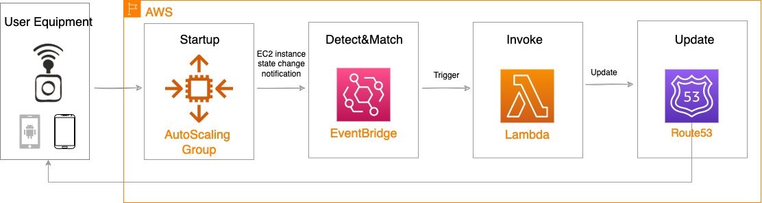


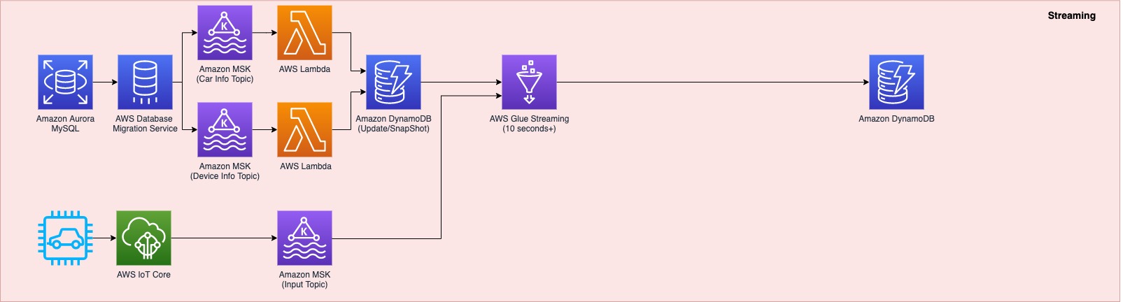
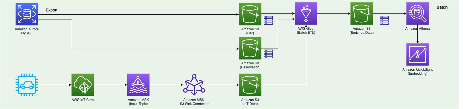
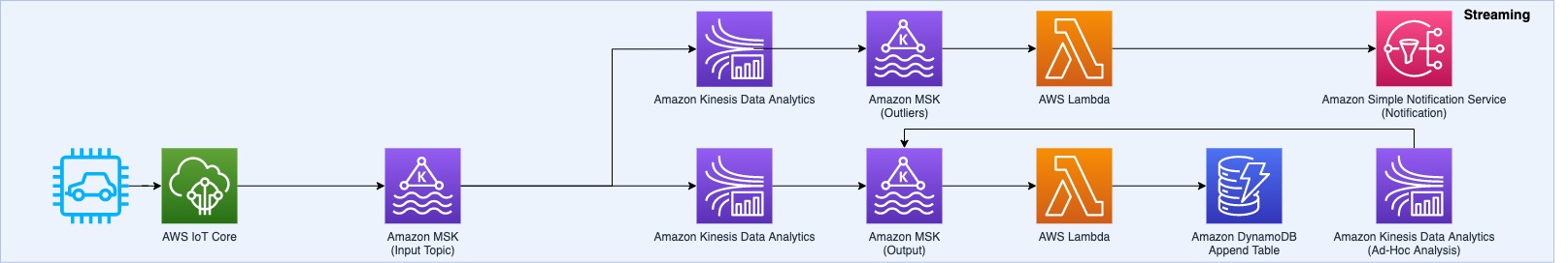


 DoYeun Kim is the Head of Data Engineering at SOCAR. He is a passionate software engineering professional with 19+ years experience. He leads a team of 10+ engineers who are responsible for the data platform, data warehouse and MLOps engineering, as well as building in-house data products.
 SangSu Park is a Lead Data Architect in SOCAR’s cloud DB team. His passion is to keep learning, embrace challenges, and strive for mutual growth through communication. He loves to travel in search of new cities and places.
 YoungMin Park is a Lead Architect in SOCAR’s cloud infrastructure team. His philosophy in life is-whatever it may be-to challenge, fail, learn, and share such experiences to build a better tomorrow for the world. He enjoys building expertise in various fields and basketball.
 Younggu Yun is a Senior Data Lab Architect at AWS. He works with customers around the APAC region to help them achieve business goals and solve technical problems by providing prescriptive architectural guidance, sharing best practices, and building innovative solutions together. In his free time, his son and he are obsessed with Lego blocks to build creative models.
 Vicky Falconer leads the AWS Data Lab program across APAC, offering accelerated joint engineering engagements between teams of customer builders and AWS technical resources to create tangible deliverables that accelerate data analytics modernization and machine learning initiatives.

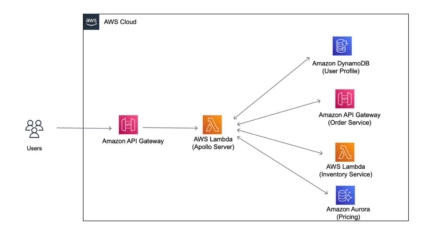
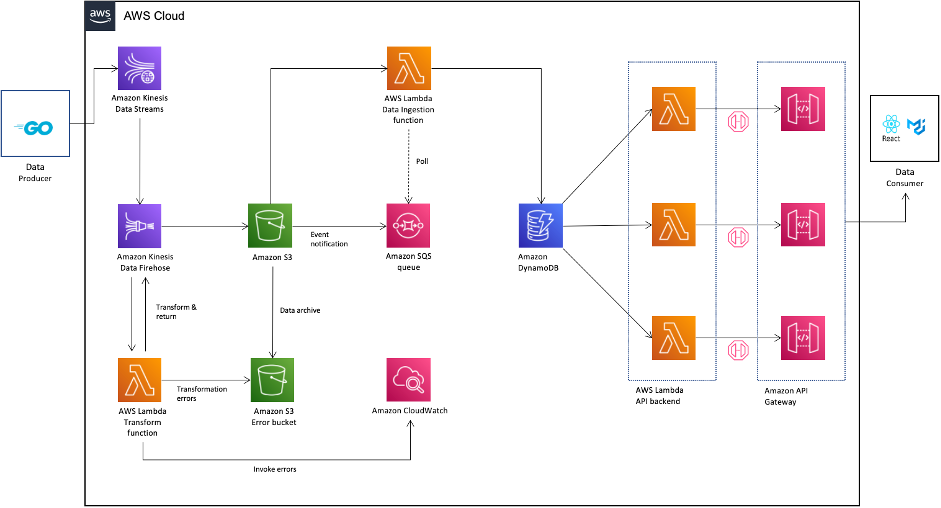


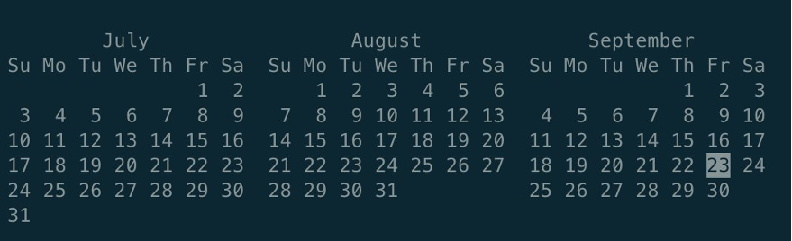
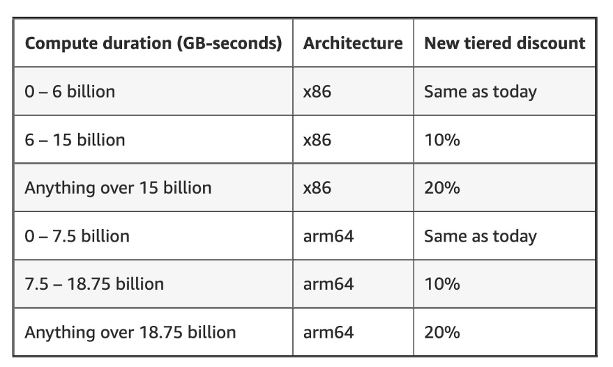

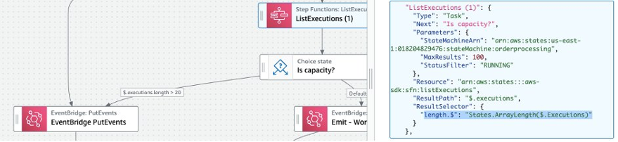


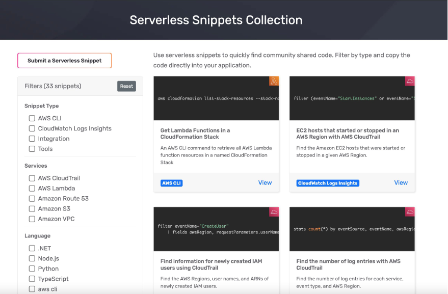
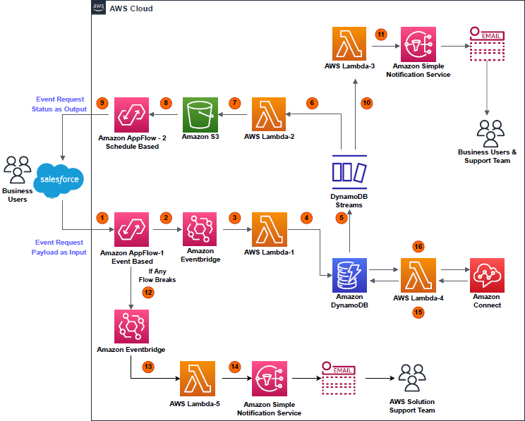
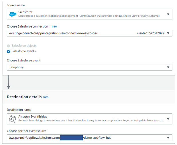
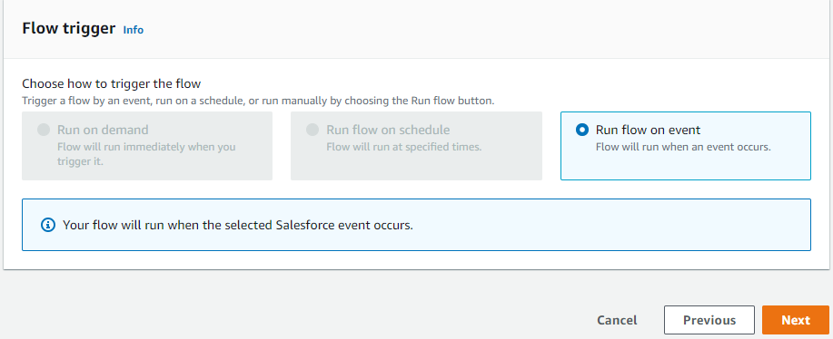
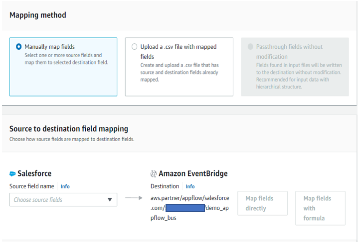
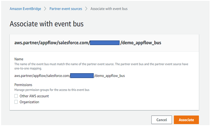
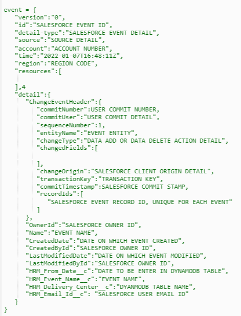
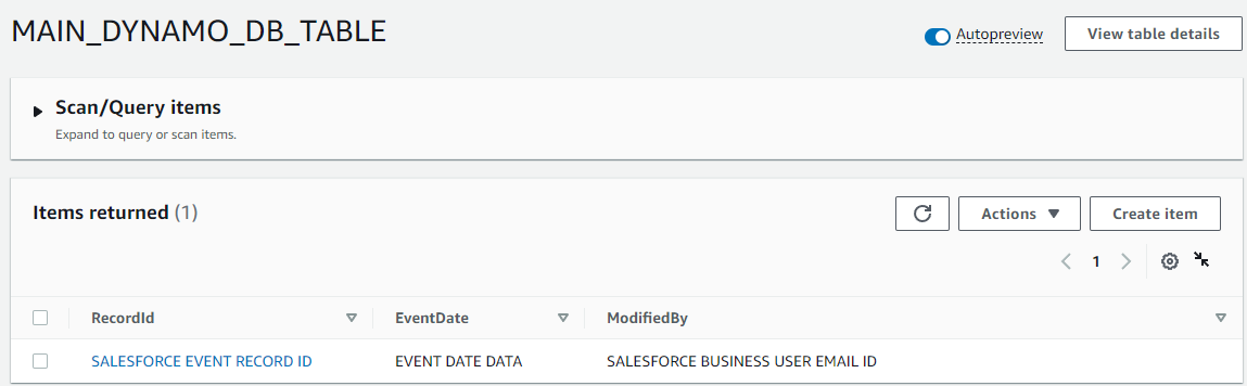
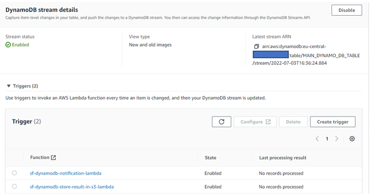
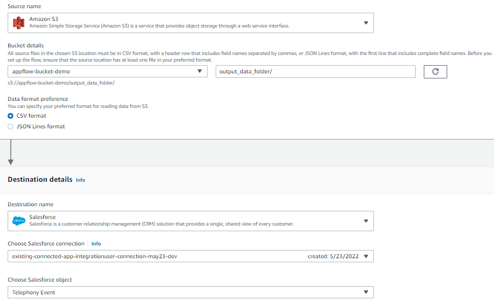
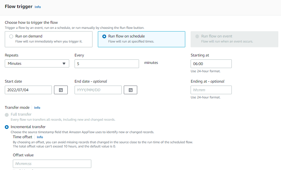
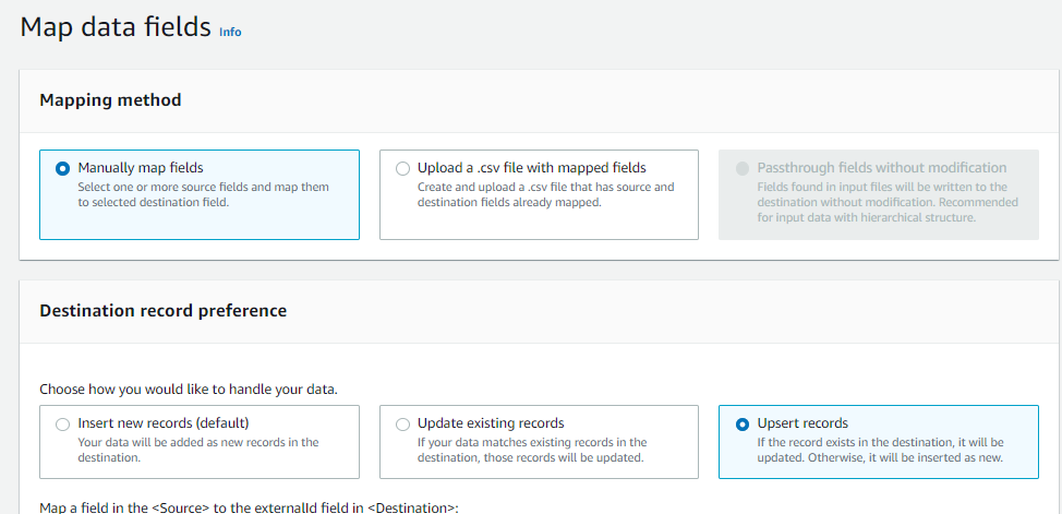


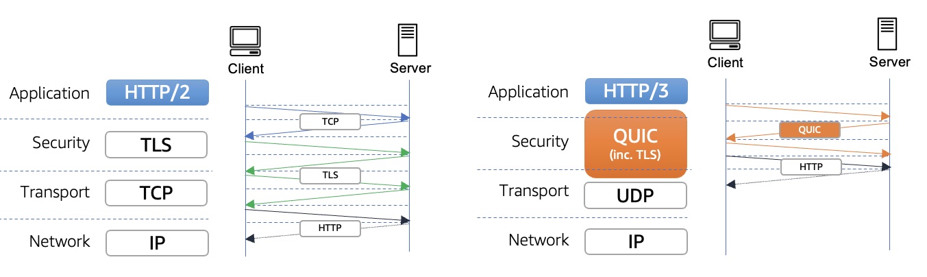


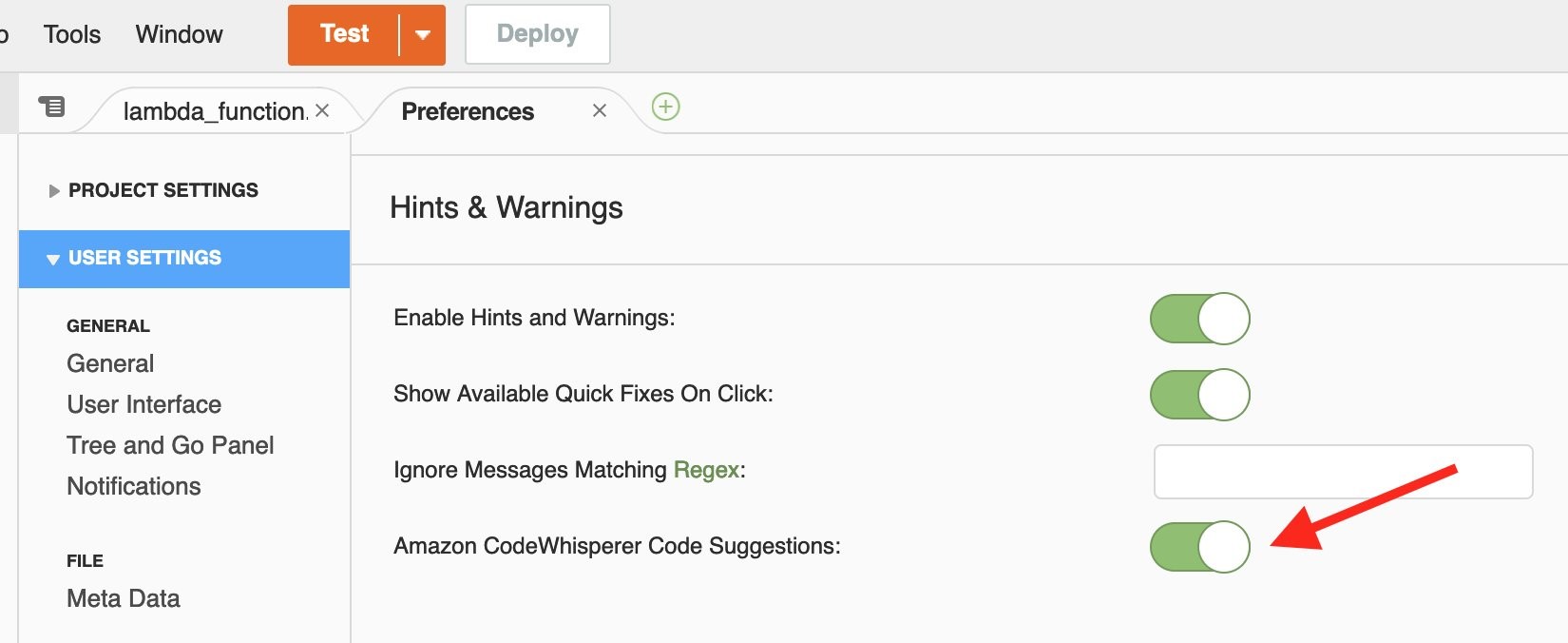

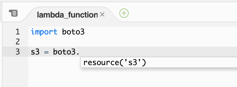


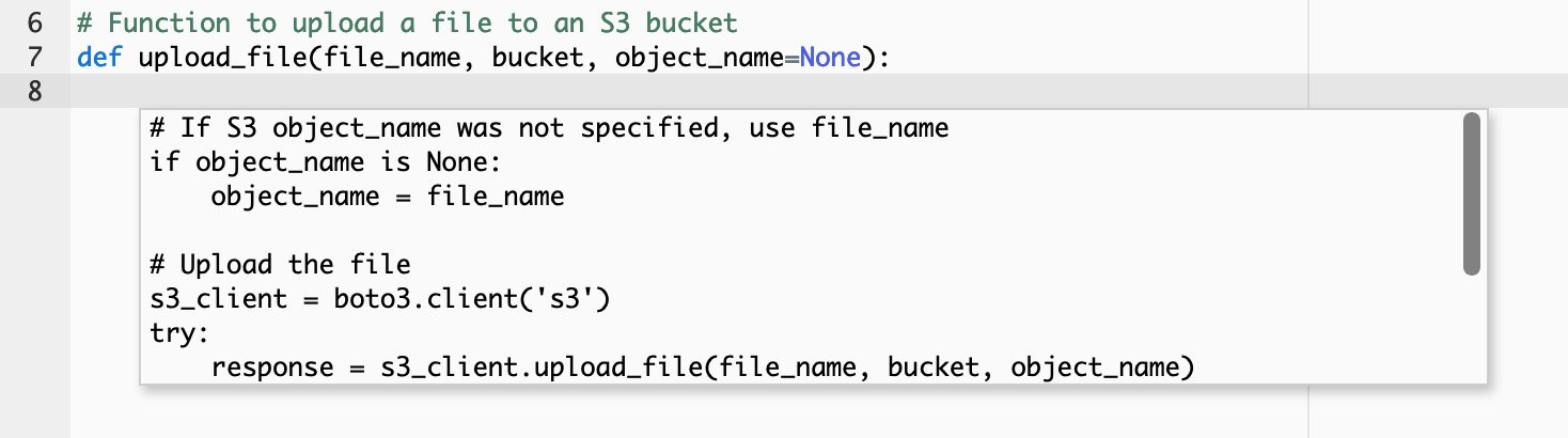

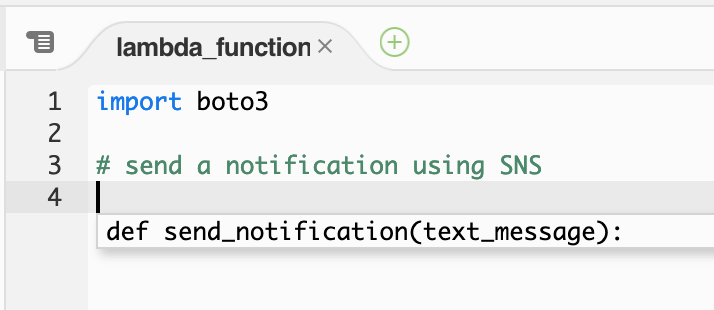

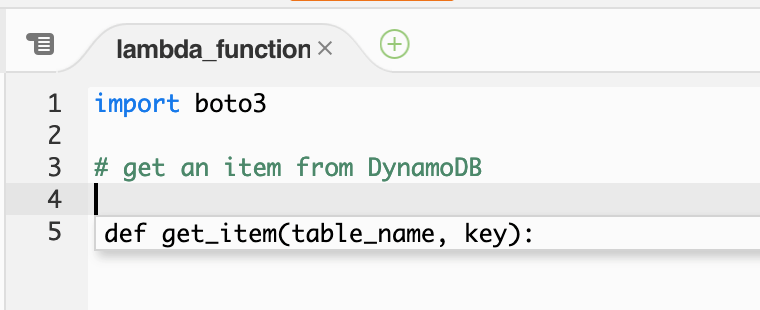

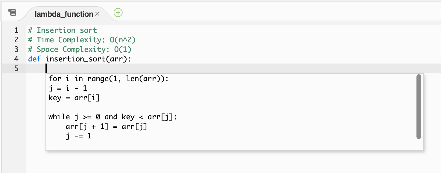

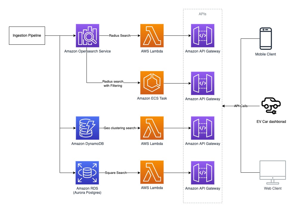
 Anand Shah is a Big Data Prototyping Solution Architect at AWS. He works with AWS customers and their engineering teams to build prototypes using AWS Analytics services and purpose-built databases. Anand helps customers solve the most challenging problems using art-of-the-possible technology. He enjoys beaches in his leisure time.