Post Syndicated from Lakshmi Nair original https://aws.amazon.com/blogs/big-data/connect-share-and-query-where-your-data-sits-using-amazon-sagemaker-unified-studio/
The ability for organizations to quickly analyze data across multiple sources is crucial for maintaining a competitive advantage. Imagine a scenario where the retail analytics team is trying to answer a simple question: Among customers who purchased summer jackets last season, which customers are likely to be interested in the new spring collection?
While the question is straightforward, getting the answer requires piecing together data across multiple data sources such as customer profiles stored in Amazon Simple Storage Service (Amazon S3) from customer relationship management (CRM) systems, historical purchase transactions in an Amazon Redshift data warehouse, and current product catalog information in Amazon DynamoDB. Traditionally, answering this question would involve multiple data exports, complex extract, transform, and load (ETL) processes, and careful data synchronization across systems.
In this blog post, we will demonstrate how business units can use Amazon SageMaker Unified Studio to discover, subscribe to, and analyze these distributed data assets. Through this unified query capability, you can create comprehensive insights into customer transaction patterns and purchase behavior for active products without the traditional barriers of data silos or the need to copy data between systems.
SageMaker Unified Studio provides a unified experience for using data, analytics, and AI capabilities. You can use familiar AWS services for model development, generative AI, data processing, and analytics—all within a single, governed environment. To strike a fine balance of democratizing data and AI access while maintaining strict compliance and regulatory standards, Amazon SageMaker Data and AI Governance is built into SageMaker Unified Studio. With Amazon SageMaker Catalog, teams can collaborate through projects, discover, and access approved data and models using semantic search with generative AI-created metadata, or you can use natural language to ask Amazon Q to find your data. Within SageMaker Unified Studio, organizations can implement a single, centralized permission model with fine-grained access controls, facilitating seamless data and AI asset sharing through streamlined publishing and subscription workflows. Teams can also query the data directly from sources such as Amazon S3 and Amazon Redshift, through Amazon SageMaker Lakehouse.
SageMaker Lakehouse streamlines connecting to, cataloging, and managing permissions on data from multiple sources. Built on AWS Glue Data Catalog and AWS Lake Formation, it organizes data through catalogs that can be accessed through an open, Apache Iceberg REST API to help ensure secure access to data with consistent, fine-grained access controls. SageMaker Lakehouse organizes data access through two types of catalogs: federated catalogs and managed catalogs (shown in the following figure). A catalog is a logical container that organizes objects from a data store, such as schemas, tables, views, or materialized views such as from Amazon Redshift. You can also create nested catalogs to mirror the hierarchical structure of your data sources within SageMaker Lakehouse.

- Federated catalogs: Through SageMaker Unified Studio, you can create connections to external data sources such as Amazon DynamoDB. See Data connections in Amazon SageMaker Lakehouse for all the supported external data sources. These connections are stored in the AWS Glue Data Catalog (Data Catalog) and registered with Lake Formation, allowing you to create a federated catalog for each available data source.
- Managed catalogs: A managed catalog refers to the data that resides on Amazon S3 or Redshift Managed Storage (RMS).
The existing Data Catalog becomes the Default catalog (identified by the AWS account number) and is readily available in SageMaker Lakehouse.
If the business units don’t have a data warehouse but need the benefits of one—such as a query result cache and query rewrite optimizations—then, they can create an RMS managed catalog in SageMaker Unified Studio. This is a SageMaker Lakehouse managed catalog backed by RMS storage. The table metadata is managed by Data Catalog. When you create an RMS managed catalog, it deploys an Amazon Redshift managed serverless workgroup. Users can write data to managed RMS tables using Iceberg APIs, Amazon Redshift, or Zero-ETL ingestion from supported data sources.
Functional working model
In SageMaker Unified Studio, the infrastructure team will enable the blueprints and configure the project profiles for tools and technologies to the respective business units to build and monitor their pipelines. They will also onboard the teams to SageMaker Unified Studio, enabling them to build the data products in a single integrated, governed environment. To enforce standardization within the organization, the central governance team can also create hierarchical representations of business units through domain units and dictate certain actions that these teams can perform under a domain unit. Global policies such as data dictionaries (business glossaries), data classification tags, and additional information with metadata forms can be created by the governance team to ensure standardization and consistency within the organization.
Individual business units will use these project profiles based on their needs to process the data using the authorized tool of their choice and create data products. Business units can enjoy the full flexibility to process and consume the data without worrying about the maintenance of the underlying infrastructure. Depending on the nature of the workloads, business units can choose a storage solution that best fits their use case. You can use SageMaker Lakehouse to unify the data across different data sources.
To share the data outside the business unit, the teams will publish the metadata of their data to a SageMaker catalog and make it discoverable and accessible to other business units. Amazon SageMaker Catalog serves as a central repository hub to store both technical and business catalog information of the data product. To establish trust between the data producers and data consumers, SageMaker Catalog also integrates the data quality metrics and data lineage events to track and drive transparency in data pipelines. While sharing the data, data producers of these business units can apply fine grained access control permissions at row and column level to these assets during subscription approval workflows. SageMaker Unified Studio automatically grants subscription access to the subscribed data assets after the subscription request is approved by the data producer. As shown in the following figure, the data sharing capability highlights that the data remains at its origin with the data producer, while consumers from other business units can consume and analyze it using their own compute resources. This approach eliminates any data duplication or data movement.

Solution overview
In this post, we explore two scenarios for sharing data between different teams (retail, marketing, and data analysts). The solution in this post gives you the implementation for a single account use case.
Scenario 1
The retail team needs to create a comprehensive view of customer behavior to optimize their spring collection launch. Their data landscape is diverse:
- Customer profiles stored in Amazon S3 (default Data Catalog)
- Historical purchase transactions stored in RMS (SageMaker Lakehouse managed RMS catalog)
- Inventory information of the product in DynamoDB. (federated catalog)
The team needs to share this unified view with their regional data analysts while maintaining strict data governance protocols. Data analysts discover the data and subscribe to the data. We will also walk through the publishing and subscription workflow as part of the data sharing process. To get a unified view of the customer sales transactions for active products, the data analysts will use Amazon Athena.

Here are the high level steps of the solution implementation as shown in the preceding diagram:
- In this post, we take an example of two teams who participate in the collaboration. The retail team has created a project
retailsales-sql-project and the data analysts team has created a project dataanalyst-sql-project within SageMaker Unified Studio.
- The retail team creates and stores their data in various sources:
customer data in Amazon S3 (contains customer data)inventory data in a DynamoDB table (contains product catalog information)store_sales_lakehouse in SageMaker Lakehouse managed RMS (contains purchase history)
- The retail team publishes the assets to the project catalog to make them discoverable to other domain members within the organization.
- The data analysts team discovers the data and subscribes to the data assets.
- An incoming request is sent to the retail team, who then approves the subscription request. After the subscription is approved, data analysts use Athena to create a unified query from all the subscribed data assets to get insights into the data.
In this scenario, we will review how SageMaker Catalog manages the subscription grants to Data Catalog assets (both federated and managed).
For this scenario, we assume that the retail team doesn’t have their own data warehouse and they want to create and manage Amazon Redshift tables using Data Catalog.
Scenario 2
The marketing team needs access to transaction data for campaign optimization. They have campaign performance data stored in an Amazon Redshift data warehouse. However, to have improved campaign ROI and better resource allocation, they need data from the retail team to understand actual customer purchase behavior. To improve the campaign ROI, they need answers to crucial questions such as:
- What is the true conversion rate across different customer segments?
- Which customers should be targeted for upcoming promotions?
- How do seasonal buying patterns affect campaign success?

Here the retail team shares the purchase history data store_sales to the marketing team. In this scenario, shown in the preceding figure, we assume that the retail team has their own data warehouse and uses Amazon Redshift to store the purchase history data.
The high level steps of the solution implementation for this scenario are:
- The marketing team has created the project
marketing-sql-project within SageMaker Unified Studio.
- The retail team has
store_sales in Amazon Redshift data warehouse (contains purchase history)
- The retail team has published the assets to the project catalog
- The marketing team discovers the data and subscribes to the data assets.
- An incoming request is sent to the retail team, who then approves the subscription request. After the subscription is approved, the marketing team uses Amazon Redshift to consume the purchase history and identify high-value customer segments.
In this scenario, we will review the process of how SageMaker Catalog grants access to managed Amazon Redshift assets.
Prerequisites
To follow the step by step guide, you must complete the following prerequisites:
Note that the default SQL analytics project profile provides you with a RedshiftServerless blueprint. However, in this post, we want to showcase the data sharing capabilities of different types of SageMaker Lakehouse catalogs (managed and federated).
For the simplicity, we chose the SQL analytics project profile. However, you can also test this by using the Custom project profile by selecting specific blueprints such as LakehouseCatalog and LakeHouseDatabase for scenarios where the business unit doesn’t have their own data warehouse.
Solution walkthrough (Scenario 1)
The first step focuses on preparing the data for each data source for unified access.
Data preparation
In this section, you will create the following data sets:
customer data in Amazon S3 (default Data Catalog)inventory data in a DynamoDB table (federated catalog)store_sales_lakehouse in SageMaker Lakehouse managed RMS (managed catalog)
- Sign in to SageMaker Unified Studio as a member of the retail team and select the project
retailsales-sql-project.
- On the top menu, choose Build, and under DATA ANALYSIS & INTEGRATION, select Query Editor.

- Select the following options:
- Under CONNECTIONS, select
Athena (Lakehouse).
- Under CATALOGS, select
AwsDataCatalog.
- Under DATABASES, select
glue_db_<environmentid> or the customer glue database name you provided during project creation.
- After the options are selected, choose Choose.

When users select a project profile within SageMaker Unified Studio, the system automatically triggers the relevant AWS CloudFormation stack (DataZone-Env-<environmentid>) and deploys the necessary infrastructure resources in the form of environments. Environments are the actual data infrastructure behind a project.
- Run the following SQL:
CREATE TABLE customer AS
SELECT 13251813 cust_id,'Joyce Deaton'   cust_name,'Greece'   cust_country, '[email protected]'   cust_email
UNION
SELECT 1581546  ,'Daniel Dow'  ,'India'  , '[email protected]'
UNION
SELECT 1581536  ,'Marie Lange'  ,'Canada'  , '[email protected]'
UNION
SELECT 1827661  ,'Wesley Harris'  ,'Rome'  , '[email protected]'
UNION
SELECT 1581536  ,'Alexander Salyer'  ,'Germany'  , '[email protected]'
UNION
SELECT 3581536  ,'Jerry Tracy'  ,'Swiss'  , '[email protected]'
- After the SQL is executed, you will find that the
customer table has been created in the Lakehouse section under Lakehouse/AwsDataCatalog/glue_db_<environmentid>.

- The product catalog is stored in DynamoDB. You can create a new table named
inventory in DynamoDB with partition key prod_id through AWS CloudShell with the following command:
aws dynamodb create-table \
    --table-name inventory\
    --attribute-definitions \
AttributeName=prod_id,AttributeType=N \
    --key-schema \
AttributeName=prod_id,KeyType=HASH \
    --provisioned-throughput \
ReadCapacityUnits=5,WriteCapacityUnits=5 \
    --table-class STANDARD
- Populate the DynamoDB table using the following commands:
aws dynamodb put-item --table-name inventory --item '{"prod_id": {"N": "1"}, "prod_name": {"S": "Widget A"},"active": {"S": "Y"}}'

aws dynamodb put-item --table-name inventory --item '{"prod_id": {"N": "2"}, "prod_name": {"S": "Gadget B"},"active": {"S": "Y"}}'

aws dynamodb put-item --table-name inventory --item '{"prod_id": {"N": "3"}, "prod_name": {"S": "Item C"},"active": {"S": "N"}}'
- To use the DynamoDB table in SageMaker Unified Studio, you need to configure a resource-based policy that allows the appropriate actions for the project role.
- To create the resource-based policy, navigate to the DynamoDB console and choose Tables from the navigation pane.
- Select the Permissions table and choose Create table policy.

- The following is an example policy that allows connecting to DynamoDB tables as a federated source. Replace the
<aws_region> with the Region you are working on, <aws_account_id> with the AWS Account ID where DynamoDB is deployed, <dynamodb_table> with the DynamoDB table (in this case inventory) that you intend to query from Amazon SageMaker Unified Studio and <datazone_usr_role_xxxxxxxxxxxxxx_yyyyyyyyyyyyyy> with the Project role Amazon Resource Name (ARN) in SageMaker Unified Studio portal. You can get the project role ARN by navigating to the project in SageMaker Unified Studio and then to Project overview.


{
    "Version": "2012-10-17",
    "Statement": [
        {
            "Effect": "Allow",
            "Principal": "*",
            "Action": [
                "dynamodb:Query",
                "dynamodb:Scan",
                "dynamodb:DescribeTable",
                "dynamodb:PartiQLSelect",
                "dynamodb:BatchWriteItem"
            ],
            "Resource": "arn:aws:dynamodb:<aws_region>:<aws_accountid>:table/<dynamodb_table>",
            "Condition": {
                "ArnEquals": {
                    "aws:PrincipalArn": "arn:aws:iam::<aws_accountid>:role/<datazone_usr_role_xxxxxxxxxxxxxx_yyyyyyyyyyyyyy>"
                }
            }
        }
    ]
}
After the policies are incorporated on the DynamoDB table, create an SageMaker Lakehouse connection within SageMaker Unified Studio. As shown in the example, dynamodb-connection-catalogs is created.

- After the connection is successfully established, you will see the DynamoDB table
inventory under Lakehouse.

The next step is to create a managed catalog for RMS objects using SageMaker Lakehouse.
- Choose Data in the navigation pane.
- In the data explorer, choose the plus icon to add a data source.
- Select Create Lakehouse catalog.
- Choose Next.

- Enter the name of the catalog. The catalog name provided in the example is
redshift-lakehouse-connection-catalogs. Choose Add data.

- After the connection is created, you will see the catalog under Lakehouse.

- This creates a managed Amazon Redshift Serverless workgroup in your AWS account. You will see a new database
dev@<redshift-catalog-name> in the managed Amazon Redshift Serverless workgroup.
- On the top menu, choose Build, and under DATA ANALYSIS & INTEGRATION, select Query Editor.
- Select Redshift (Lakehouse) from CONNECTIONS,
dev@<redshift-catalog-name> from DATABASES and public from SCHEMAS

- Run the following SQL in order. The SQL creates the
store_sales_lakehouse table in the dev database in the public schema. The retail team inserts data into the store_sales_lakehouse table.
CREATE TABLE public.store_sales_lakehouse (
    sale_id INTEGER IDENTITY(1,1) PRIMARY KEY,
    cust_id INTEGER NOT NULL,
    sale_date DATE NOT NULL,
    sale_amount DECIMAL(10, 2) NOT NULL,
    prod_id INTEGER  NOT NULL,
    last_purchase_date DATE
);
INSERT INTO public.store_sales_lakehouse (cust_id, sale_date, sale_amount, prod_id, last_purchase_date)
VALUES
(13251813, '2023-01-15', 150.00, 1, '2023-01-15'),
(29033279, '2023-01-20', 200.00, 4, '2023-01-20'),
(12755125, '2023-02-01', 75.50, 3, '2023-02-01'),
(26009249, '2023-02-10', 300.00, 2, '2023-02-10'),
(3270685, '2023-02-15', 125.00, 2, '2023-02-15'),
(6520539, '2023-03-01', 100.00, 2, '2023-03-01'),
(10251183, '2023-03-10', 250.00, 1, '2023-03-10'),
(10251283, '2023-03-15', 180.00, 1, '2023-03-15'),
(10251383, '2023-04-01', 90.00, 2, '2023-04-01'),
(10251483, '2023-04-10', 220.00, 3, '2023-04-10'),
(10251583, '2023-04-15', 175.00, 3, '2023-04-15'),
(10251683, '2023-05-01', 130.00, 1, '2023-05-01'),
(10251783, '2023-05-10', 280.00, 1, '2023-05-10'),
(10251883, '2023-05-15', 195.00, 4, '2023-05-15'),
(10251983, '2023-06-01', 110.00, 2, '2023-06-01'),
(10251083, '2023-06-10', 270.00, 1, '2023-06-10'),
(10252783, '2023-06-15', 185.00, 2, '2023-06-15'),
(10253783, '2023-07-01', 95.00, 3, '2023-07-01'),
(10254783, '2023-07-10', 240.00, 1, '2023-07-10'),
(10255783, '2023-07-15', 160.00, 3, '2023-07-15');
- On successful creation of the table, you should now be able to query the data. Select the table
store_sales_lakehouse and select Query with Redshift.

Import assets to the project catalog from various data sources
To share your assets outside your own project to other business units, you must first bring your metadata to SageMaker Catalog. To import the assets into the project’s inventory, you need to create a data source in the project catalog. In this section, we show you how to import the technical metadata from AWS Glue data catalogs. Here, you will import data assets from various sources that you have created as part of your data preparation.
- Sign in to SageMaker Unified Studio as a member of the retail team. Select the project
retailsales-sql-project, under Project catalog. Choose Data sources and import the assets by choosing Run.


- To import the federated catalog, create a new data source and choose Run. This will import the metadata of the inventory data from DynamoDB table.
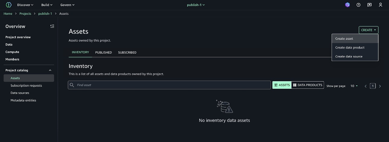
- After successful run of all the data sources, choose Assets under Project catalog in the navigation plane. You will find all the assets in the Inventory of Project catalog.

Publish the assets
To make the assets discoverable to the data analysts team, the retail team must publish their assets.
- In the project
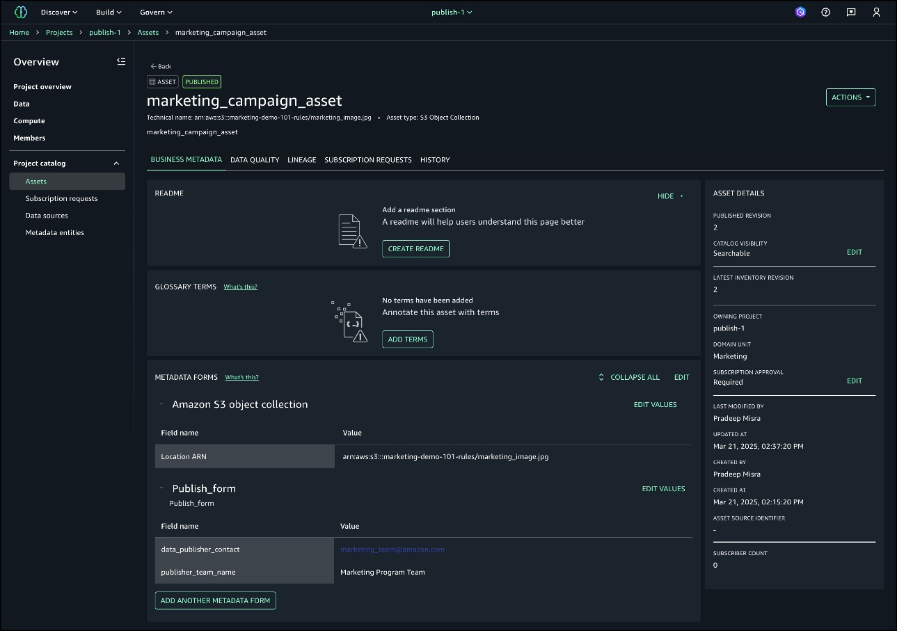
retailsales-sql-project, choose Project catalog and select Assets.
- Select each asset in the INVENTORY tab, enrich the asset with the automated metadata generation and PUBLISH ASSET.
Discover the assets
SageMaker Catalog within SageMaker Unified Studio enables efficient data asset discovery and access management. The data analysts team signs in to SageMaker Unified Studio and selects the project dataanalyst-sql-project. The data analysts team then locates the desired assets in SageMaker Catalog and initiates the subscription request.
In this section, members of dataanalyst-sql-project browse the catalog and find the assets. There are multiple ways to find the desired assets.
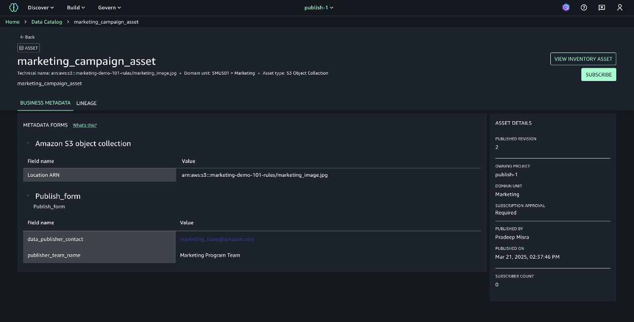
- Sign in to SageMaker Unified Studio as a member of the data analysts team. Choose Discover in the top navigation bar and select Catalog. Find the desired asset by browsing or entering the name of the asset into the search bar.
- Search for the asset through a conversational interface using Amazon Q.
- Use the faceted filter search by selecting the desired project in the BROWSE CATALOG.

The data analysts team selects the project retailsales-sql-project.

Subscribe to the assets
The data analysts team submits a subscription request with an appropriate justification for each of these assets.
- For each asset, choose SUBSCRIBE.
- Select
dataanalyst-sql-project in Project.
- Provide the Reason for request as “need this data for analysis”.
Note that during the subscription process, the requester sees a message that the asset access control and fulfillment will be Managed. This means that SageMaker Unified Studio automatically manages subscription access grants and permissions for these assets.
Subscription approval workflow
To approve the subscription request, you must be a member of the retail team and select the project that has published the asset.
- Sign in to SageMaker Unified Studio as a member of the retail team and select the project
retailsales-sql-project.
- In the navigation pane, choose Project catalog and then select Subscription requests.
- In INCOMING REQUESTS, choose the REQUESTED tab and select View request for each asset to see detailed information of the subscription request.

- REQUEST DETAILS provides information about the subscribing project, the requestor, and the justification to access the asset.
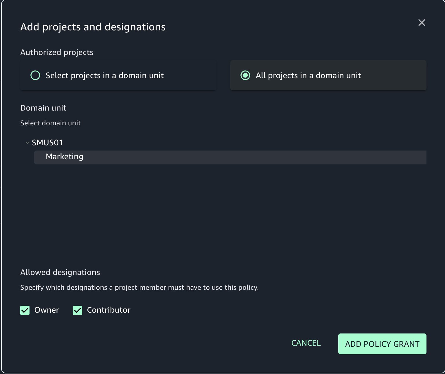
- RESPONSE DETAILS provides an option to approve the subscription with full access to the data (Full access) or restricted access to the data (Approve with row or column filters). With restricted access to data, the subscription approval workflow process offers granular access control for sensitive data through row-level filtering and column-level filtering. Using row filters, approvers can restrict access to specific records based on defined criteria. Using column filters, approvers can control access to specific columns within the data sets. This allows excluding sensitive fields while sharing the relevant data. Approvers can implement these filters during the approval process, helping to ensure that the data access aligns with the organization’s security requirements and compliance policies. For this post, select Full access in the RESPONSE DETAILS
- (Optional) Decision comment is where you can add a comment about accepting or rejecting the subscription request.
- Choose APPROVE.

- Repeat the subscription approval workflow process for all the requested assets.
- After all the subscription requests are approved, choose the APPROVED tab to view all the approved assets.

Subscription fulfillment methods
After subscription approval, a fulfillment process manages access to the assets. SageMaker Unified Studio provides fulfillment methods for managed assets and unmanaged assets.
- Managed assets: SageMaker Unified Studio automatically manages the fulfillment and permissions for assets such as AWS Glue tables and Amazon Redshift tables and views.
- Unmanaged assets: For unmanaged assets, permissions are handled externally. SageMaker Unified Studio publishes standard events for actions such as approvals through Amazon EventBridge, enabling integration with other AWS services or third-party solutions for custom integrations.
In this scenario 1, because the assets are Data Catalogs, SageMaker Unified Studio grants and manages access to these managed assets on your behalf through Lake Formation. See the SageMaker Unified Studio subscription workflow for updates on sharing options.
Analyze the data
The data analysts team uses the subscribed data assets from varied sources to get unified insights.
- As a data analyst, sign in to SageMaker Unified Studio and select the project
dataanalyst-sql-project. In the navigation pane, choose Project catalog and select Assets.
- Choose the SUBSCRIBED tab to find all the subscribed assets from the
retailsales-sql-project.
- The status under each asset is
Asset accessible. This indicates that the subscription grants are fulfilled and the data analysts team can now consume the assets with the compute of their choice.

Query using Athena (subscription grants fulfilled using Lake Formation)
As a member of the data analysts team, create a unified view to get purchase history with customer information for active products.
- In the
dataanalyst-sql-project project, go to Build and select Query Editor.
- Use the following sample query to get the required information. Replace
glue_db_<environmentid> with your subscribed glue database.
select * from "redshift-lakehouse-connection-catalogs/dev"."public"."store_sales_lakehouse" sales
 left  join "awsdatacatalog"."glue_db_<environmentid>"."customer" customer
 on sales.cust_id=customer.cust_id
 inner  join "dynamodb-connection-catalogs"."default"."inventory" inventory
 on sales.prod_id = inventory.prod_id
 where inventory.active ='Y'

Solution walk-through (Scenario 2)
In this scenario, we assume that the retail team stores the purchase history data in their Amazon Redshift data warehouse. Because you’re using the default SQL analytics project profile to create the project, you will use a Redshift Serverless compute (project.redshift). The purchase history data is shared with the marketing team for enhanced campaign performance.
- Sign in to SageMaker Unified Studio as a member of the retail team and select the project
retailsales-sql-project.
- On the top menu, choose Build, and under DATA ANALYSIS & INTEGRATION, select Query Editor
- Select the following options:
- Under CONNECTIONS, select
Redshift(Lakehouse).
- Under CATALOGS, select
dev.
- Under DATABASES, select
public.
- Run the following SQL:
CREATE TABLE public.store_sales (
sale_id INTEGER IDENTITY(1,1) PRIMARY KEY,
cust_id INTEGER NOT NULL,
sale_date DATE NOT NULL,
sale_amount DECIMAL(10, 2) NOT NULL,
prod_id INTEGER  NOT NULL,
last_purchase_date DATE
);
INSERT INTO public.store_sales (cust_id, sale_date, sale_amount, prod_id, last_purchase_date)
VALUES
(13251813, '2023-01-15', 150.00, 1, '2023-01-15'),
(29033279, '2023-01-20', 200.00, 4, '2023-01-20'),
(12755125, '2023-02-01', 75.50, 3, '2023-02-01'),
(26009249, '2023-02-10', 300.00, 2, '2023-02-10'),
(3270685, '2023-02-15', 125.00, 2, '2023-02-15'),
(6520539, '2023-03-01', 100.00, 2, '2023-03-01'),
(10251183, '2023-03-10', 250.00, 1, '2023-03-10'),
(10251283, '2023-03-15', 180.00, 1, '2023-03-15'),
(10251383, '2023-04-01', 90.00, 2, '2023-04-01'),
(10251483, '2023-04-10', 220.00, 3, '2023-04-10'),
(10251583, '2023-04-15', 175.00, 3, '2023-04-15'),
(10251683, '2023-05-01', 130.00, 1, '2023-05-01'),
(10251783, '2023-05-10', 280.00, 1, '2023-05-10'),
(10251883, '2023-05-15', 195.00, 4, '2023-05-15'),
(10251983, '2023-06-01', 110.00, 2, '2023-06-01'),
(10251083, '2023-06-10', 270.00, 1, '2023-06-10'),
(10252783, '2023-06-15', 185.00, 2, '2023-06-15'),
(10253783, '2023-07-01', 95.00, 3, '2023-07-01'),
(10254783, '2023-07-10', 240.00, 1, '2023-07-10'),
(10255783, '2023-07-15', 160.00, 3, '2023-07-15');
5. On successful execution of the query, you will see store_sales under Redshift in the navigation pane.

Import the asset to the project catalog inventory
To share your assets outside your own project to other marketing business units, you must first share your metadata to SageMaker Catalog. To import the assets into the project’s inventory, you need to run the data source in the project catalog.
In the project retailsales-sql-project, under Project catalog, select Data sources and import the asset store-sales. Select the highlighted data source and choose Run as shown in the screenshot.

Publish the asset
To make the assets discoverable to the marketing team, the retail team must publish their asset.
- Go to the navigation pane and choose Project catalog, and then select Assets.
- Select
store-sales in the INVENTORY tab, enrich the asset with the automated metadata generation and PUBLISH ASSET as illustrated in the screenshot.
Discover and subscribe the asset
The marketing team discovers and subscribes to the store-sales asset.
- Sign in to SageMaker Unified Studio as a member of the marketing team and select
marketing-sql-project.
- Navigate to the Discover menu in the top navigation bar and choose Catalog. Find the desired asset by browsing or entering the name of the asset into the search bar.
- Select the asset and choose SUBSCRIBE.
- Enter a justification in Reason for request and choose REQUEST.
Subscription approval workflow
The retail team gets an incoming request in their project to approve the subscription request.
- Sign in to the SageMaker Unified Studio and select the project
retailsales-sql-project as a member of the retail team. Under Project catalog, select Subscription requests.
- In the INCOMING REQUESTS, under the REQUESTED tab, select View request for
store-sales.

- You will see detailed information for the subscription request.
- Select Full access in the RESPONSE DETAILS and choose APPROVE.

Analyze the data
Sign in to SageMaker Unified Studio as a member of the marketing team and select marketing-sql-project.
- In the Project catalog, select Assets and choose the SUBSCRIBED tab to find all the subscribed assets from the
retailsales-sql-project.
- Notice the status under the asset marked as
Asset accessible. This indicates that the subscription grants are fulfilled and the marketing team can now consume the asset with the compute of their choice.

Query using Amazon Redshift (subscription grants fulfilled using native Amazon Redshift data sharing)
To query the shared data with Amazon Redshift compute, select Build and then Query Editor. Select the following options
- Under CONNECTIONS, select
Redshift(Lakehouse).
- Under CATALOGS, select
dev.
- Under DATABASES, select
project.
select * from "dev"."project"."store_sales" sales

When a subscription to an Amazon Redshift table or view is approved, SageMaker Unified Studio automatically adds the subscribed asset to the consumer’s Amazon Redshift Serverless workgroup for the project. Notice the subscribed asset is shared under the folder project. In the Redshift navigation pane, you can also see the datashare created between the source and the target cluster. In this case, because the data is shared in the same account but between different clusters, SageMaker Unified Studio creates a view in the target database and permissions are granted on the view. See Grant access to managed Amazon Redshift assets in Amazon SageMaker Unified Studio for information about data sharing options within Amazon Redshift.
Clean up
Make sure you remove the SageMaker Unified Studio resources to avoid any unexpected costs. Start by deleting the connections, catalogs, underlying data sources, projects, databases, and domain that you created for this post. For additional details, see the Amazon SageMaker Unified Studio Administrator Guide.
Conclusion
In this post, we explored two distinct approaches to data sharing and analytics.
Business units without an existing data warehouse can use a SageMaker Lakehouse managed RMS catalog. In the first scenario, we showcased subscription fulfillment of AWS Glue Data Catalogs using AWS Lake Formation for federated and managed catalogs. The data analysts team was able to connect and subscribe to the data shared by the retail team that resided in Amazon S3, Amazon Redshift, and other data sources such as DynamoDB through SageMaker Lakehouse.
In the second scenario, we demonstrated the native data-sharing capabilities of Amazon Redshift. In this scenario, we assume that the retail team has sales transactions stored in an Amazon Redshift data warehouse. Using the data sharing feature of Amazon Redshift, the asset was shared to the marketing team using Amazon SageMaker Unified Studio.
Both approaches enable unified querying across varied data sources with teams able to efficiently discover, publish, and subscribe to data assets while maintaining strict access controls through Amazon SageMaker Data and AI Governance. Subscription fulfillment is automated, reducing the administrative overhead. Using the query-in-place approach eliminates data redundancy and maintains data consistency while allowing unified analysis across data sources through a single integrated experience.
To learn more, see the Amazon SageMaker Unified Studio Administrator Guide and the following resources:
About the authors
 Lakshmi Nair is a Senior Analytics Specialist Solutions Architect at AWS. She specializes in designing advanced analytics systems across industries. She focuses on crafting cloud-based data platforms, enabling real-time streaming, big data processing, and robust data governance. She can be reached through LinkedIn
 Ramkumar Nottath is a Principal Solutions Architect at AWS focusing on Analytics services. He enjoys working with various customers to help them build scalable, reliable big data and analytics solutions. His interests extend to various technologies such as analytics, data warehousing, streaming, data governance, and machine learning. He loves spending time with his family and friends.


 Suba Palanisamy is a Senior Technical Account Manager helping customers achieve operational excellence using AWS. Suba is passionate about all things data and analytics. She enjoys traveling with her family and playing board games
 Anubhav Gupta is a Solutions Architect at AWS supporting enterprise greenfield customers, focusing on the financial services industry. He has worked with hundreds of customers worldwide building their cloud foundational environments and platforms, architecting new workloads, and creating governance strategy for their cloud environments. In his free time, he enjoys traveling and spending time outdoors
 Anusha Pininti is a Solutions Architect guiding enterprise greenfield customers through every stage of their cloud transformation, specializing in data analytics. She supports customers across various industries, helping them achieve their business objectives through cloud-based solutions. In her free time, Anusha loves to travel, spend time with family, and experiment with new dishes
 Sriharsh Adari is a Senior Solutions Architect at AWS, where he helps customers work backward from business outcomes to develop innovative solutions on AWS. Over the years, he has helped multiple customers on data platform transformations across industry verticals. His core area of expertise includes technology strategy, data analytics, and data science. In his spare time, he enjoys playing sports, watching TV shows, and playing Tabla
 Geetha Penmatsa is a Solutions Architect supporting enterprise greenfield customers through their cloud journey. She helps customers across various industries transform their business with the AWS Cloud. She has a background in data analytics and is specializing in Amazon Connect Cloud contact center to help transform customer experience at scale. Outside work, Geetha loves to travel, ski, hike, and spend time with friends and family


 Pradeep Misra is a Principal Analytics Solutions Architect at AWS. He works across Amazon to architect and design modern distributed analytics and AI/ML platform solutions. He is passionate about solving customer challenges using data, analytics, and AI/ML. Outside of work, Pradeep likes exploring new places, trying new cuisines, and playing board games with his family. He also likes doing science experiments, building LEGOs and watching anime with his daughters.
 Ramesh H Singh is a Senior Product Manager Technical (External Services) at AWS in Seattle, Washington, currently with the Amazon SageMaker team. He is passionate about building high-performance ML/AI and analytics products that enable enterprise customers to achieve their critical goals using cutting-edge technology. Connect with him on
  Sandhya Edupuganti is a Senior Engineering Leader spearheading Amazon DataZone (aka) SageMaker Catalog. She is based in Seattle Metro area and has been with Amazon for over 17 years leading strategic initiatives in Amazon Advertising, Amazon-Retail, Latam-Expansion and AWS Analytics.


 Deepmala Agarwal works as an AWS Data Specialist Solutions Architect. She is passionate about helping customers build out scalable, distributed, and data-driven solutions on AWS. When not at work, Deepmala likes spending time with family, walking, listening to music, watching movies, and cooking!
 Flavio Torres is a Principal Technical Account Manager at AWS. Flavio helps Enterprise Support customers design, deploy, and scale resilient cloud applications. Outside of work, he enjoys hiking and barbecuing.


 Subramanya Vajiraya is a Sr. Cloud Engineer (ETL) at AWS Sydney specialized in AWS Glue. He is passionate about helping customers solve issues related to their ETL workload and implementing scalable data processing and analytics pipelines on AWS. Outside of work, he enjoys going on bike rides and taking long walks with his dog Ollie.
 Noritaka Sekiyama is a Principal Big Data Architect on the AWS Glue team. He works based in Tokyo, Japan. He is responsible for building software artifacts to help customers. In his spare time, he enjoys cycling with his road bike.


