Post Syndicated from Navnit Shukla original https://aws.amazon.com/blogs/big-data/process-and-analyze-highly-nested-and-large-xml-files-using-aws-glue-and-amazon-athena/
In today’s digital age, data is at the heart of every organization’s success. One of the most commonly used formats for exchanging data is XML. Analyzing XML files is crucial for several reasons. Firstly, XML files are used in many industries, including finance, healthcare, and government. Analyzing XML files can help organizations gain insights into their data, allowing them to make better decisions and improve their operations. Analyzing XML files can also help in data integration, because many applications and systems use XML as a standard data format. By analyzing XML files, organizations can easily integrate data from different sources and ensure consistency across their systems, However, XML files contain semi-structured, highly nested data, making it difficult to access and analyze information, especially if the file is large and has complex, highly nested schema.
XML files are well-suited for applications, but they may not be optimal for analytics engines. In order to enhance query performance and enable easy access in downstream analytics engines such as Amazon Athena, it’s crucial to preprocess XML files into a columnar format like Parquet. This transformation allows for improved efficiency and usability in analytics workflows. In this post, we show how to process XML data using AWS Glue and Athena.
Solution overview
We explore two distinct techniques that can streamline your XML file processing workflow:
- Technique 1: Use an AWS Glue crawler and the AWS Glue visual editor – You can use the AWS Glue user interface in conjunction with a crawler to define the table structure for your XML files. This approach provides a user-friendly interface and is particularly suitable for individuals who prefer a graphical approach to managing their data.
- Technique 2: Use AWS Glue DynamicFrames with inferred and fixed schemas – The crawler has a limitation when it comes to processing a single row in XML files larger than 1 MB. To overcome this restriction, we use an AWS Glue notebook to construct AWS Glue
DynamicFrames, utilizing both inferred and fixed schemas. This method ensures efficient handling of XML files with rows exceeding 1 MB in size.
In both approaches, our ultimate goal is to convert XML files into Apache Parquet format, making them readily available for querying using Athena. With these techniques, you can enhance the processing speed and accessibility of your XML data, enabling you to derive valuable insights with ease.
Prerequisites
Before you begin this tutorial, complete the following prerequisites (these apply to both techniques):
- Download the XML files technique1.xml and technique2.xml.
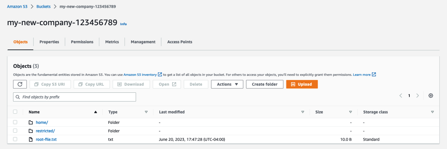
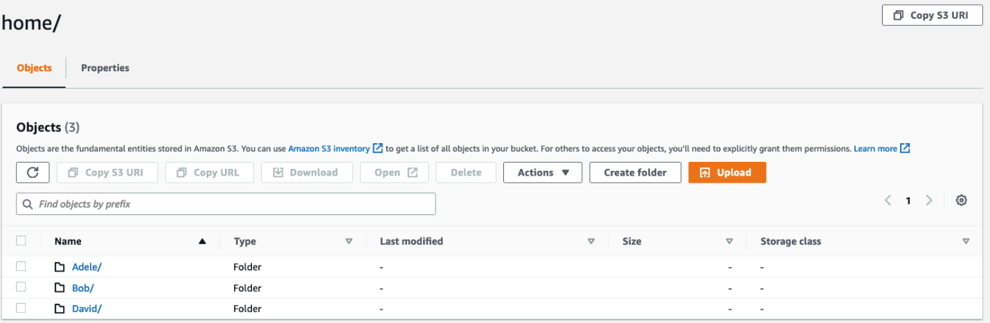
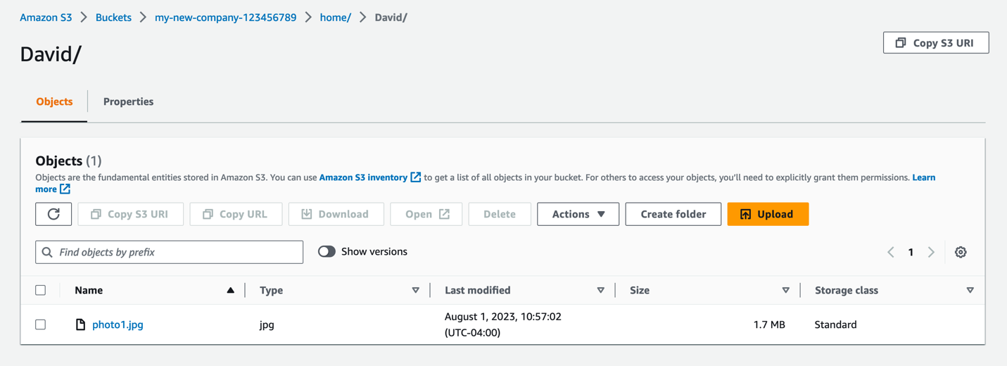
- Upload the files to an Amazon Simple Storage Service (Amazon S3) bucket. You can upload them to the same S3 bucket in different folders or to different S3 buckets.
- Create an AWS Identity and Access Management (IAM) role for your ETL job or notebook as instructed in Set up IAM permissions for AWS Glue Studio.
- Add an inline policy to your role with the iam:PassRole action:
  "Version": "2012-10-17",
  "Statement": [
    {
      "Action": ["iam:PassRole"],
      "Effect": "Allow",
      "Resource": "arn:aws:iam::*:role/AWSGlueServiceRole*",
      "Condition": {
        "StringLike": {
          "iam:PassedToService": ["glue.amazonaws.com"]
        }
      }
    }
}
- Add a permissions policy to the role with access to your S3 bucket.
Now that we’re done with the prerequisites, let’s move on to implementing the first technique.
Technique 1: Use an AWS Glue crawler and the visual editor
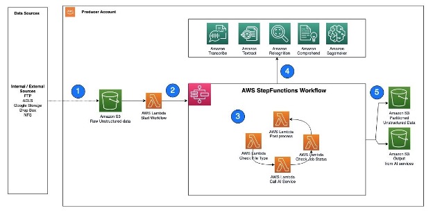
The following diagram illustrates the simple architecture that you can use to implement the solution.

To analyze XML files stored in Amazon S3 using AWS Glue and Athena, we complete the following high-level steps:
- Create an AWS Glue crawler to extract XML metadata and create a table in the AWS Glue Data Catalog.
- Process and transform XML data into a format (like Parquet) suitable for Athena using an AWS Glue extract, transform, and load (ETL) job.
- Set up and run an AWS Glue job via the AWS Glue console or the AWS Command Line Interface (AWS CLI).
- Use the processed data (in Parquet format) with Athena tables, enabling SQL queries.
- Use the user-friendly interface in Athena to analyze the XML data with SQL queries on your data stored in Amazon S3.
This architecture is a scalable, cost-effective solution for analyzing XML data on Amazon S3 using AWS Glue and Athena. You can analyze large datasets without complex infrastructure management.
We use the AWS Glue crawler to extract XML file metadata. You can choose the default AWS Glue classifier for general-purpose XML classification. It automatically detects XML data structure and schema, which is useful for common formats.
We also use a custom XML classifier in this solution. It’s designed for specific XML schemas or formats, allowing precise metadata extraction. This is ideal for non-standard XML formats or when you need detailed control over classification. A custom classifier ensures only necessary metadata is extracted, simplifying downstream processing and analysis tasks. This approach optimizes the use of your XML files.
The following screenshot shows an example of an XML file with tags.

Create a custom classifier
In this step, you create a custom AWS Glue classifier to extract metadata from an XML file. Complete the following steps:
- On the AWS Glue console, under Crawlers in the navigation pane, choose Classifiers.
- Choose Add classifier.
- Select XML as the classifier type.
- Enter a name for the classifier, such as
blog-glue-xml-contact.
- For Row tag, enter the name of the root tag that contains the metadata (for example,
metadata).
- Choose Create.

Create an AWS Glue Crawler to crawl xml file
In this section, we are creating a Glue Crawler to extract the metadata from XML file using the customer classifier created in previous step.
Create a database
- Go to the AWS Glue console, choose Databases in the navigation pane.
- Click on Add database.
- Provide a name such as
blog_glue_xml
- Choose Create Database
Create a Crawler
Complete the following steps to create your first crawler:
- On the AWS Glue console, choose Crawlers in the navigation pane.
- Choose Create crawler.
- On the Set crawler properties page, provide a name for the new crawler (such as
blog-glue-parquet), then choose Next.
- On the Choose data sources and classifiers page, select Not Yet under Data source configuration.
- Choose Add a data store.
- For S3 path, browse to
s3://${BUCKET_NAME}/input/geologicalsurvey/.
Make sure you pick the XML folder rather than the file inside the folder.
- Leave the rest of the options as default and choose Add an S3 data source.
- Expand Custom classifiers – optional, choose blog-glue-xml-contact, then choose Next and keep the rest of the options as default.
- Choose your IAM role or choose Create new IAM role, add the suffix
glue-xml-contact (for example, AWSGlueServiceNotebookRoleBlog), and choose Next.
- On the Set output and scheduling page, under Output configuration, choose
blog_glue_xml for Target database.
- Enter
console_ as the prefix added to tables (optional) and under Crawler schedule, keep the frequency set to On demand.
- Choose Next.
- Review all the parameters and choose Create crawler.
Run the Crawler
After you create the crawler, complete the following steps to run it:
- On the AWS Glue console, choose Crawlers in the navigation pane.
- Open the crawler you created and choose Run.
The crawler will take 1–2 minutes to complete.

- When the crawler is complete, choose Databases in the navigation pane.
- Choose the database you crated and choose the table name to see the schema extracted by the crawler.

Create an AWS Glue job to convert the XML to Parquet format
In this step, you create an AWS Glue Studio job to convert the XML file into a Parquet file. Complete the following steps:
- On the AWS Glue console, choose Jobs in the navigation pane.
- Under Create job, select Visual with a blank canvas.
- Choose Create.
- Rename the job to
blog_glue_xml_job.
Now you have a blank AWS Glue Studio visual job editor. On the top of the editor are the tabs for different views.
- Choose the Script tab to see an empty shell of the AWS Glue ETL script.
As we add new steps in the visual editor, the script will be updated automatically.
- Choose the Job details tab to see all the job configurations.
- For IAM role, choose
AWSGlueServiceNotebookRoleBlog.
- For Glue version, choose Glue 4.0 – Support Spark 3.3, Scala 2, Python 3.
- Set Requested number of workers to 2.
- Set Number of retries to 0.
- Choose the Visual tab to go back to the visual editor.
- On the Source drop-down menu, choose AWS Glue Data Catalog.
- On the Data source properties – Data Catalog tab, provide the following information:
- For Database, choose
blog_glue_xml.
- For Table, choose the table that starts with the name console_ that the crawler created (for example,
console_geologicalsurvey).
- On the Node properties tab, provide the following information:
- Change Name to
geologicalsurvey dataset.
- Choose Action and the transformation Change Schema (Apply Mapping).
- Choose Node properties and change the name of the transform from Change Schema (Apply Mapping) to
ApplyMapping.
- On the Target menu, choose S3.
- On the Data source properties – S3 tab, provide the following information:
- For Format, select Parquet.
- For Compression Type, select Uncompressed.
- For S3 source type, select S3 location.
- For S3 URL, enter
s3://${BUCKET_NAME}/output/parquet/.
- Choose Node Properties and change the name to
Output.
- Choose Save to save the job.
- Choose Run to run the job.
The following screenshot shows the job in the visual editor.

Create an AWS Gue Crawler to crawl the Parquet file
In this step, you create an AWS Glue crawler to extract metadata from the Parquet file you created using an AWS Glue Studio job. This time, you use the default classifier. Complete the following steps:
- On the AWS Glue console, choose Crawlers in the navigation pane.
- Choose Create crawler.
- On the Set crawler properties page, provide a name for the new crawler, such as blog-glue-parquet-contact, then choose Next.
- On the Choose data sources and classifiers page, select Not Yet for Data source configuration.
- Choose Add a data store.
- For S3 path, browse to
s3://${BUCKET_NAME}/output/parquet/.
Make sure you pick the parquet folder rather than the file inside the folder.
- Choose your IAM role created during the prerequisite section or choose Create new IAM role (for example,
AWSGlueServiceNotebookRoleBlog), and choose Next.
- On the Set output and scheduling page, under Output configuration, choose
blog_glue_xml for Database.
- Enter
parquet_ as the prefix added to tables (optional) and under Crawler schedule, keep the frequency set to On demand.
- Choose Next.
- Review all the parameters and choose Create crawler.
Now you can run the crawler, which takes 1–2 minutes to complete.

You can preview the newly created schema for the Parquet file in the AWS Glue Data Catalog, which is similar to the schema of the XML file.

We now possess data that is suitable for use with Athena. In the next section, we perform data queries using Athena.
Query the Parquet file using Athena
Athena doesn’t support querying the XML file format, which is why you converted the XML file into Parquet for more efficient data querying and use dot notation to query complex types and nested structures.
The following example code uses dot notation to query nested data:
SELECT
    idinfo.citation.citeinfo.origin,
    idinfo.citation.citeinfo.pubdate,
    idinfo.citation.citeinfo.title,
    idinfo.citation.citeinfo.geoform,
    idinfo.citation.citeinfo.pubinfo.pubplace,
    idinfo.citation.citeinfo.pubinfo.publish,
    idinfo.citation.citeinfo.onlink,
    idinfo.descript.abstract,
    idinfo.descript.purpose,
    idinfo.descript.supplinf,
    dataqual.attracc.attraccr,
    dataqual.logic,
    dataqual.complete,
    dataqual.posacc.horizpa.horizpar,
    dataqual.posacc.vertacc.vertaccr,
    dataqual.lineage.procstep.procdate,
    dataqual.lineage.procstep.procdesc
FROM "blog_glue_xml"."parquet_parquet" limit 10;

Now that we’ve completed technique 1, let’s move on to learn about technique 2.
Technique 2: Use AWS Glue DynamicFrames with inferred and fixed schemas
In the previous section, we covered the process of handling a small XML file using an AWS Glue crawler to generate a table, an AWS Glue job to convert the file into Parquet format, and Athena to access the Parquet data. However, the crawler encounters limitations when it comes to processing XML files that exceed 1 MB in size. In this section, we delve into the topic of batch processing larger XML files, necessitating additional parsing to extract individual events and conduct analysis using Athena.
Our approach involves reading the XML files through AWS Glue DynamicFrames, employing both inferred and fixed schemas. Then we extract the individual events in Parquet format using the relationalize transformation, enabling us to query and analyze them seamlessly using Athena.
To implement this solution, you complete the following high-level steps:
- Create an AWS Glue notebook to read and analyze the XML file.
- Use
DynamicFrames with InferSchema to read the XML file.
- Use the relationalize function to unnest any arrays.
- Convert the data to Parquet format.
- Query the Parquet data using Athena.
- Repeat the previous steps, but this time pass a schema to
DynamicFrames instead of using InferSchema.
The electric vehicle population data XML file has a response tag at its root level. This tag contains an array of row tags, which are nested within it. The row tag is an array that contains a set of another row tags, which provide information about a vehicle, including its make, model, and other relevant details. The following screenshot shows an example.

Create an AWS Glue Notebook
To create an AWS Glue notebook, complete the following steps:
- Open the AWS Glue Studio console, choose Jobs in the navigation pane.
- Select Jupyter Notebook and choose Create.

- Enter a name for your AWS Glue job, such as
blog_glue_xml_job_Jupyter.
- Choose the role that you created in the prerequisites (
AWSGlueServiceNotebookRoleBlog).

The AWS Glue notebook comes with a preexisting example that demonstrates how to query a database and write the output to Amazon S3.
- Adjust the timeout (in minutes) as shown in the following screenshot and run the cell to create the AWS Glue interactive session.

Create basic Variables
After you create the interactive session, at the end of the notebook, create a new cell with the following variables (provide your own bucket name):
BUCKET_NAME='YOUR_BUCKET_NAME'
S3_SOURCE_XML_FILE = f's3://{BUCKET_NAME}/xml_dataset/'
S3_TEMP_FOLDER = f's3://{BUCKET_NAME}/temp/'
S3_OUTPUT_INFER_SCHEMA = f's3://{BUCKET_NAME}/infer_schema/'
INFER_SCHEMA_TABLE_NAME = 'infer_schema'
S3_OUTPUT_NO_INFER_SCHEMA = f's3://{BUCKET_NAME}/no_infer_schema/'
NO_INFER_SCHEMA_TABLE_NAME = 'no_infer_schema'
DATABASE_NAME = 'blog_xml'
Read the XML file inferring the schema
If you don’t pass a schema to the DynamicFrame, it will infer the schema of the files. To read the data using a dynamic frame, you can use the following command:
df = glueContext.create_dynamic_frame.from_options(
    connection_type="s3",
    connection_options={"paths": [S3_SOURCE_XML_FILE]},
    format="xml",
    format_options={"rowTag": "response"},
)
Print the DynamicFrame Schema
Print the schema with the following code:

The schema shows a nested structure with a row array containing multiple elements. To unnest this structure into lines, you can use the AWS Glue relationalize transformation:
df_relationalized = df.relationalize(
    "root", S3_TEMP_FOLDER
)
We are only interested in the information contained within the row array, and we can view the schema by using the following command:
df_relationalized.select("root_row.row").printSchema()

The column names contain row.row, which correspond to the array structure and array column in the dataset. We don’t rename the columns in this post; for instructions to do so, refer to Automate dynamic mapping and renaming of column names in data files using AWS Glue: Part 1. Then you can convert the data to Parquet format and create the AWS Glue table using the following command:
s3output = glueContext.getSink(
  path= S3_OUTPUT_INFER_SCHEMA,
  connection_type="s3",
  updateBehavior="UPDATE_IN_DATABASE",
  partitionKeys=[],
  compression="snappy",
  enableUpdateCatalog=True,
  transformation_ctx="s3output",
)
s3output.setCatalogInfo(
  catalogDatabase="blog_xml", catalogTableName="jupyter_notebook_with_infer_schema"
)
s3output.setFormat("glueparquet")
s3output.writeFrame(df_relationalized.select("root_row.row"))
AWS Glue DynamicFrame provides features that you can use in your ETL script to create and update a schema in the Data Catalog. We use the updateBehavior parameter to create the table directly in the Data Catalog. With this approach, we don’t need to run an AWS Glue crawler after the AWS Glue job is complete.

Read the XML file by setting a schema
An alternative way to read the file is by predefining a schema. To do this, complete the following steps:
- Import the AWS Glue data types:
from awsglue.gluetypes import *
- Create a schema for the XML file:
schema = StructType([
  Field("row", StructType([
    Field("row", ArrayType(StructType([
            Field("_2020_census_tract", LongType()),
            Field("__address", StringType()),
            Field("__id", StringType()),
            Field("__position", IntegerType()),
            Field("__uuid", StringType()),
            Field("base_msrp", IntegerType()),
            Field("cafv_type", StringType()),
            Field("city", StringType()),
            Field("county", StringType()),
            Field("dol_vehicle_id", IntegerType()),
            Field("electric_range", IntegerType()),
            Field("electric_utility", StringType()),
            Field("ev_type", StringType()),
            Field("geocoded_column", StringType()),
            Field("legislative_district", IntegerType()),
            Field("make", StringType()),
            Field("model", StringType()),
            Field("model_year", IntegerType()),
            Field("state", StringType()),
            Field("vin_1_10", StringType()),
            Field("zip_code", IntegerType())
    ])))
  ]))
])
- Pass the schema when reading the XML file:
df = glueContext.create_dynamic_frame.from_options(
    connection_type="s3",
    connection_options={"paths": [S3_SOURCE_XML_FILE]},
    format="xml",
    format_options={"rowTag": "response", "withSchema": json.dumps(schema.jsonValue())},
)
- Unnest the dataset like before:
df_relationalized = df.relationalize(
    "root", S3_TEMP_FOLDER
)
- Convert the dataset to Parquet and create the AWS Glue table:
s3output = glueContext.getSink(
  path=S3_OUTPUT_NO_INFER_SCHEMA,
  connection_type="s3",
  updateBehavior="UPDATE_IN_DATABASE",
  partitionKeys=[],
  compression="snappy",
  enableUpdateCatalog=True,
  transformation_ctx="s3output",
)
s3output.setCatalogInfo(
  catalogDatabase="blog_xml", catalogTableName="jupyter_notebook_no_infer_schema"
)
s3output.setFormat("glueparquet")
s3output.writeFrame(df_relationalized.select("root_row.row"))
Query the tables using Athena
Now that we have created both tables, we can query the tables using Athena. For example, we can use the following query:
SELECT * FROM "blog_xml"."jupyter_notebook_no_infer_schema " limit 10;
The following screenshot shows the results.

Clean Up
In this post, we created an IAM role, an AWS Glue Jupyter notebook, and two tables in the AWS Glue Data Catalog. We also uploaded some files to an S3 bucket. To clean up these objects, complete the following steps:
- On the IAM console, delete the role you created.
- On the AWS Glue Studio console, delete the custom classifier, crawler, ETL jobs, and Jupyter notebook.
- Navigate to the AWS Glue Data Catalog and delete the tables you created.
- On the Amazon S3 console, navigate to the bucket you created and delete the folders named
temp, infer_schema, and no_infer_schema.
Key Takeaways
In AWS Glue, there’s a feature called InferSchema in AWS Glue DynamicFrames. It automatically figures out the structure of a data frame based on the data it contains. In contrast, defining a schema means explicitly stating how the data frame’s structure should be before loading the data.
XML, being a text-based format, doesn’t restrict the data types of its columns. This can cause issues with the InferSchema function. For example, in the first run, a file with column A having a value of 2 results in a Parquet file with column A as an integer. In the second run, a new file has column A with the value C, leading to a Parquet file with column A as a string. Now there are two files on S3, each with a column A of different data types, which can create problems downstream.
The same happens with complex data types like nested structures or arrays. For example, if a file has one tag entry called transaction, it’s inferred as a struct. But if another file has the same tag, it’s inferred as an array
Despite these data type issues, InferSchema is useful when you don’t know the schema or defining one manually is impractical. However, it’s not ideal for large or constantly changing datasets. Defining a schema is more precise, especially with complex data types, but has its own issues, like requiring manual effort and being inflexible to data changes.
InferSchema has limitations, like incorrect data type inference and issues with handling null values. Defining a schema also has limitations, like manual effort and potential errors.
Choosing between inferring and defining a schema depends on the project’s needs. InferSchema is great for quick exploration of small datasets, whereas defining a schema is better for larger, complex datasets requiring accuracy and consistency. Consider the trade-offs and constraints of each method to pick what suits your project best.
Conclusion
In this post, we explored two techniques for managing XML data using AWS Glue, each tailored to address specific needs and challenges you may encounter.
Technique 1 offers a user-friendly path for those who prefer a graphical interface. You can use an AWS Glue crawler and the visual editor to effortlessly define the table structure for your XML files. This approach simplifies the data management process and is particularly appealing to those looking for a straightforward way to handle their data.
However, we recognize that the crawler has its limitations, specifically when dealing with XML files having rows larger than 1 MB. This is where technique 2 comes to the rescue. By harnessing AWS Glue DynamicFrames with both inferred and fixed schemas, and employing an AWS Glue notebook, you can efficiently handle XML files of any size. This method provides a robust solution that ensures seamless processing even for XML files with rows exceeding the 1 MB constraint.
As you navigate the world of data management, having these techniques in your toolkit empowers you to make informed decisions based on the specific requirements of your project. Whether you prefer the simplicity of technique 1 or the scalability of technique 2, AWS Glue provides the flexibility you need to handle XML data effectively.
About the Authors
 Navnit Shuklaserves as an AWS Specialist Solution Architect with a focus on Analytics. He possesses a strong enthusiasm for assisting clients in discovering valuable insights from their data. Through his expertise, he constructs innovative solutions that empower businesses to arrive at informed, data-driven choices. Notably, Navnit Shukla is the accomplished author of the book titled “Data Wrangling on AWS.
 Patrick Muller works as a Senior Data Lab Architect at AWS. His main responsibility is to assist customers in turning their ideas into a production-ready data product. In his free time, Patrick enjoys playing soccer, watching movies, and traveling.
 Amogh Gaikwad is a Senior Solutions Developer at Amazon Web Services. He helps global customers build and deploy AI/ML solutions on AWS. His work is mainly focused on computer vision, and natural language processing and helping customers optimize their AI/ML workloads for sustainability. Amogh has received his master’s in Computer Science specializing in Machine Learning.
 Sheela Sonone is a Senior Resident Architect at AWS. She helps AWS customers make informed choices and tradeoffs about accelerating their data, analytics, and AI/ML workloads and implementations. In her spare time, she enjoys spending time with her family – usually on tennis courts.


 Satya Adimula is a Senior Data Architect at AWS based in Boston. With over two decades of experience in data and analytics, Satya helps organizations derive business insights from their data at scale.
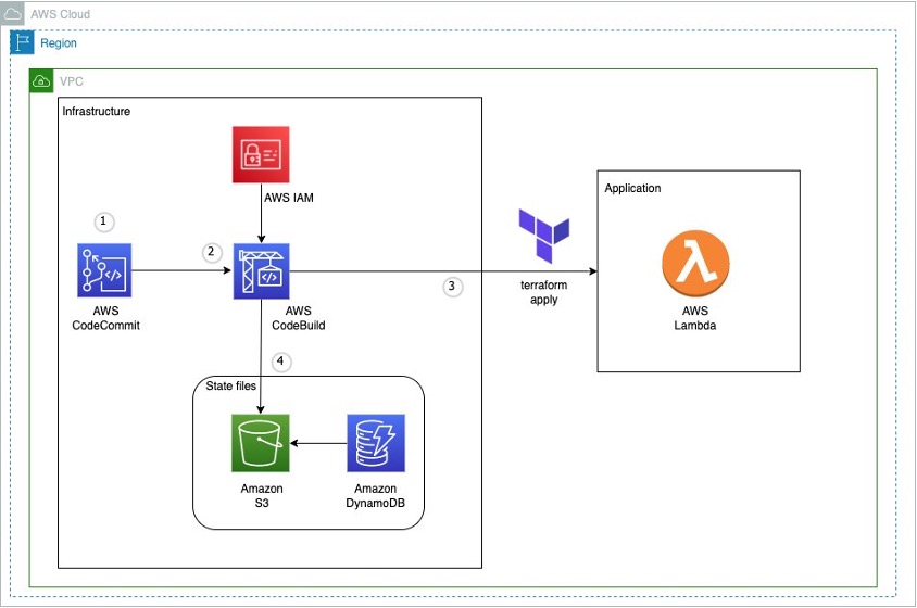


 Parnab Basak is a Senior Solutions Architect and a Serverless Specialist at AWS. He specializes in creating new solutions that are cloud native using modern software development practices like serverless, DevOps, and analytics. Parnab works closely in the analytics and integration services space helping customers adopt AWS services for their workflow orchestration needs.
 Chandan Rupakheti is a Solutions Architect and a Serverless Specialist at AWS. He is a passionate technical leader, researcher, and mentor with a knack for building innovative solutions in the cloud and bringing stakeholders together in their cloud journey. Outside his professional life, he loves spending time with his family and friends besides listening and playing music.
 Vinod Jayendra is a Enterprise Support Lead in ISV accounts at Amazon Web Services, where he helps customers in solving their architectural, operational, and cost optimization challenges. With a particular focus on Serverless technologies, he draws from his extensive background in application development to deliver top-tier solutions. Beyond work, he finds joy in quality family time, embarking on biking adventures, and coaching youth sports team.
 Rupesh Tiwari is a Senior Solutions Architect at AWS in New York City, with a focus on Financial Services. He has over 18 years of IT experience in the finance, insurance, and education domains, and specializes in architecting large-scale applications and cloud-native big data workloads. In his spare time, Rupesh enjoys singing karaoke, watching comedy TV series, and creating joyful moments with his family.


 Harman Singh Dhodi is an Analyst at HR&A Advisors, Harman combines his passion for data analytics with sustainable infrastructure practices, social inclusion, economic viability, climate resiliency, and building stakeholder capacity. Harman’s work often focuses on translating complex datasets into visual stories and accessible tools that help empower communities to understand the challenges they’re facing and create solutions for a brighter future.
 Kiran Kumar Tati is an Analytics Specialist Solutions Architect based out of Omaha, NE. He specializes in building end-to-end analytic solutions. He has more than 13 years of experience with designing and implementing large scale Big Data and Analytics solutions. In his spare time, he enjoys playing cricket and watching sports.
 Sapna Maheshwari is a Sr. Solutions Architect at Amazon Web Services. She helps customers architect data analytics solutions at scale on AWS. Outside of work she enjoys traveling and trying new cuisines.


 Kamen Sharlandjiev is a Sr. Big Data and ETL Solutions Architect and AWS Glue expert. He’s on a mission to make life easier for customers who are facing complex data integration challenges. His secret weapon? Fully managed, low-code AWS services that can get the job done with minimal effort and no coding. Follow Kamen on LinkedIn to keep up to date with the latest AWS Glue news!
 Sean Bjurstrom is a Technical Account Manager in ISV accounts at Amazon Web Services, where he specializes in analytics technologies and draws on his background in consulting to support customers on their analytics and cloud journeys. Sean is passionate about helping businesses harness the power of data to drive innovation and growth. Outside of work, he enjoys running and has participated in several marathons.
 Vinod Jayendra is an Enterprise Support Lead in ISV accounts at Amazon Web Services, where he helps customers solve their architectural, operational, and cost-optimization challenges. With a particular focus on serverless technologies, he draws from his extensive background in application development to help customers build top-tier solutions. Beyond work, he finds joy in quality family time, embarking on biking adventures, and coaching youth sports teams.
 Doug Mbaya is a Senior Partner Solution architect with a focus in analytics and machine learning. Doug works closely with AWS partners and helps them integrate their solutions with AWS analytics and machine learning solutions in the cloud.


 Damon Cortesi is a Principal Developer Advocate with Amazon Web Services. He builds tools and content to help make the lives of data engineers easier. When not hard at work, he still builds data pipelines and splits logs in his spare time.


 Sakti Mishra is a Principal Solutions Architect at AWS, where he helps customers modernize their data architecture and define their end-to-end data strategy, including data security, accessibility, governance, and more. He is also the author of the book
  Bhavana Chirumamilla is a Senior Resident Architect at AWS with a strong passion for data and machine learning operations. She brings a wealth of experience and enthusiasm to help enterprises build effective data and ML strategies. In her spare time, Bhavana enjoys spending time with her family and engaging in various activities such as traveling, hiking, gardening, and watching documentaries.
 Sheela Sonone is a Senior Resident Architect at AWS. She helps AWS customers make informed choices and trade-offs about accelerating their data, analytics, and AI/ML workloads and implementations. In her spare time, she enjoys spending time with her family—usually on tennis courts.
 Daniel Bruno is a Principal Resident Architect at AWS. He had been building analytics and machine learning solutions for over 20 years and splits his time helping customers build data science programs and designing impactful ML products.


 Gokhul Srinivasan is a Senior Partner Solutions Architect leading AWS Healthcare and Life Sciences (HCLS) Global Startup Partners. Gokhul has over 19 years of Healthcare experience helping organizations with digital transformation, platform modernization, and deliver business outcomes.
 Laks Sundararajan is a seasoned Enterprise Architect helping companies reset, transform and modernize their IT, digital, cloud, data and insight strategies. A proven leader with significant expertise around Generative AI, Digital, Cloud and Data/Analytics Transformation, Laks is a Sr. Solutions Architect with Healthcare and Life Sciences (HCLS).
 Anil Chinnam is a Solutions Architect in the Digital Native Business Segment at Amazon Web Services(AWS). He enjoys working with customers to understand their challenges and solve them by creating innovative solutions using AWS services. Outside of work, Anil enjoys being a father, swimming and traveling.


 Navnit Shuklaserves as an AWS Specialist Solution Architect with a focus on Analytics. He possesses a strong enthusiasm for assisting clients in discovering valuable insights from their data. Through his expertise, he constructs innovative solutions that empower businesses to arrive at informed, data-driven choices. Notably, Navnit Shukla is the accomplished author of the book titled “Data Wrangling on AWS.
 Patrick Muller works as a Senior Data Lab Architect at AWS. His main responsibility is to assist customers in turning their ideas into a production-ready data product. In his free time, Patrick enjoys playing soccer, watching movies, and traveling.
 Amogh Gaikwad is a Senior Solutions Developer at Amazon Web Services. He helps global customers build and deploy AI/ML solutions on AWS. His work is mainly focused on computer vision, and natural language processing and helping customers optimize their AI/ML workloads for sustainability. Amogh has received his master’s in Computer Science specializing in Machine Learning.


 available.


 Ravi Itha is a Principal Consultant at AWS Professional Services with specialization in data and analytics and generalist background in application development. Ravi helps customers with enterprise data strategy initiatives across insurance, airlines, pharmaceutical, and financial services industries. In his 6-year tenure at Amazon, Ravi has helped the AWS builder community by publishing approximately 15 open-source solutions (accessible via
  Srinivas Kandi is a Data Architect at AWS Professional Services. He leads customer engagements related to data lakes, analytics, and data warehouse modernizations. He enjoys reading history and civilizations.


 Cristiane de Melo is a Solutions Architect Manager at AWS based in Bay Area, CA. She brings 25+ years of experience driving technical pre-sales engagements and is responsible for delivering results to customers. Cris is passionate about working with customers, solving technical and business challenges, thriving on building and establishing long-term, strategic relationships with customers and partners.
 Archana Inapudi is a Senior Solutions Architect at AWS supporting Strategic Customers. She has over a decade of experience helping customers design and build data analytics, and database solutions. She is passionate about using technology to provide value to customers and achieve business outcomes.
 Nikita Sur is a Solutions Architect at AWS supporting a Strategic Customer. She is curious to learn new technologies to solve customer problems. She has a Master’s degree in Information Systems – Big Data Analytics and her passion is databases and analytics.
 Zach Mitchell is a Sr. Big Data Architect. He works within the product team to enhance understanding between product engineers and their customers while guiding customers through their journey to develop their enterprise data architecture on AWS.