Tag Archives: Customer Solutions

Create a Multi-Region Python Package Publishing Pipeline with AWS CDK and CodePipeline

2022-11-03 Brian Smitches

Post Syndicated from Brian Smitches original https://aws.amazon.com/blogs/devops/create-a-multi-region-python-package-publishing-pipeline-with-aws-cdk-and-codepipeline/

Customers can author and store internal software packages in AWS by leveraging the AWS CodeSuite (AWS CodePipeline, AWS CodeBuild, AWS CodeCommit, and AWS CodeArtifact). As of the publish date of this blog post, there is no native way to replicate your CodeArtifact Packages across regions. This blog addresses how a custom solution built with the AWS Cloud Development Kit and AWS CodePipeline can create a Multi-Region Python Package Publishing Pipeline.

Whether it’s for resiliency or performance improvement, many customers want to deploy their applications across multiple regions. When applications are dependent on custom software packages, the software packages should be replicated to multiple regions as well. This post will walk through how to deploy a custom package publishing pipeline in your own AWS Account. This pipeline connects a Python package source code repository to build and publish pip packages to CodeArtifact Repositories spanning three regions (the primary and two replica regions). While this sample CDK Application is built specifically for pip packages, the underlying architecture can be reused for different software package formats, such as npm, Maven, NuGet, etc.

Solution overview

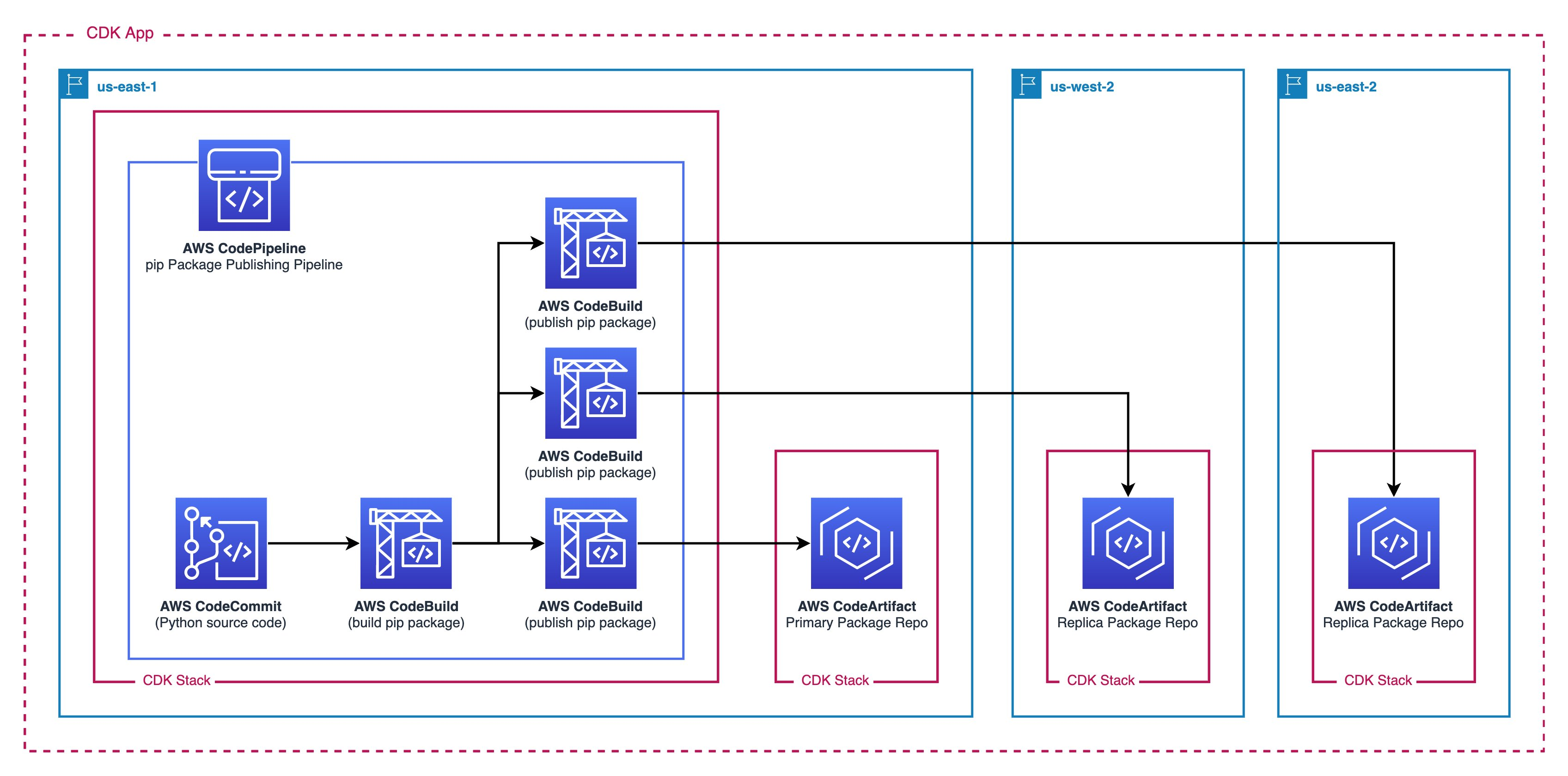
The following figure demonstrates the solution workflow:

A CodePipeline pipeline orchestrates the building and publishing of the software package

1. This pipeline is triggered by commits on the main branch of the CodeCommit repository
2. A CodeBuild job builds the pip packages using twine to be distributed
3. The publish stage (third column) uses three parallel CodeBuild jobs to publish the distribution package to the two CodeArtifact repositories in separate regions

The first CodeArtifact Repository stores the package contents in the primary region.
The second and third CodeArtifact Repository act as replicas and store the package contents in other regions.

Figure 1. A figure showing the architecture diagram

Figure 1. Architecture diagram

All of these resources are defined in a single AWS CDK Application. The resources are defined in CDK Stacks that are deployed as AWS CloudFormation Stacks. AWS CDK can deploy the different stacks across separate regions.

Prerequisites

Before getting started, you will need the following:

An AWS account
An instance of the AWS Cloud9 IDE or an alternative local compute environment, such as your personal computer
The following installed on your compute environment:

1. AWS CDK
2. AWS Command Line Interface (AWS CLI)
3. npm

The AWS Accounts must be bootstrapped for CDK in the necessary regions. The default configuration uses us-east-1, us-east-2 and us-west-2 as these three regions support CodeArtifact.

A new AWS Cloud9 IDE is recommended for this tutorial to isolate these actions in this post from your normal compute environment. See the Cloud9 Documentation for Creating an Environment.

Deploy the Python Package Publishing Pipeline into your AWS Account with the CDK

The source code can be found in this GitHub Repository.

Fork the GitHub Repo into your account. This way you can experiment with changes as necessary to fit your workload.
In your local compute environment, clone the GitHub Repository and cd into the project directory:

git clone [email protected]:<YOUR_GITHUB_USERNAME>/multi-region-
python-package-publishing-pipeline.git && cd multi-region-
python-package-publishing-pipeline

Install the necessary node packages:

npm i

(Optional) Override the default configurations for the CodeArtifact domainName, repositoryName, primaryRegion, and replicaRegions.
1. navigate to ./bin/multiregion_package_publishing.ts and update the relevant fields.
2. From the project’s root directory (multi-region-python-package-publishing-pipeline), deploy the AWS CDK application. This step may take 5-10 minutes.

cdk deploy --all

When prompted “Do you wish to deploy these changes (y/n)?”, Enter y.

Viewing the deployed CloudFormation stacks

After the deployment of the AWS CDK application completes, you can view the deployed AWS CDK Stacks via CloudFormation. From the AWS Console, search “CloudFormation’ in the search bar and navigate to the service dashboard. In the primary region (us-east-1(N. Virginia)) you should see two stacks: CodeArtifactPrimaryStack-<region> and PackagePublishingPipelineStack.

Figure 2. Screenshot showing the CloudFormation Stacks in the primary region

Switch regions to one of the secondary regions us-west-2 (Oregon) or us-east-2 (Ohio) to see the remaining stacks named CodeArtifactReplicaStack-<region>. These correspond to the three AWS CDK Stacks from the architecture diagram.

Figure 3. Screenshot showing the CloudFormation stacks in a separate region

Viewing the CodePipeline Package Publishing Pipeline

From the Console, select the primary region (us-east-1) and navigate to CodePipeline by utilizing the search bar. Select the Pipeline titled packagePipeline and inspect the state of the pipeline. This pipeline triggers after every commit from the CodeCommit repository named PackageSourceCode. If the pipeline is still in process, then wait a few minutes, as this pipeline can take approximately 7–8 minutes to complete all three stages (Source, Build, and Publish). Once it’s complete, the pipeline should reflect the following screenshot:

Figure 4. A screenshot showing the CodePipeline flow

Viewing the Published Package in the CodeArtifact Repository

To view the published artifacts, go to the primary or secondary region and navigate to the CodeArtifact dashboard by utilizing the search bar in the Console. You’ll see a repository named package-artifact-repo. Select the repository and you’ll see the sample pip package named mypippackage inside the repository. This package is defined by the source code in the CodeCommit repository named PackageSourceCode in the primary region (us-east-1).

Figure 5. Screenshot of the package repository

Create a new package version in CodeCommit and monitor the pipeline release

Navigate to your CodeCommit’s PackageSourceCode (us-east-1 CodeCommit > Repositories > PackageSourceCode. Open the setup.py file and select the Edit button. Make a simple modification, change the version = '1.0.0' to version = '1.1.0' and commit the changes to the Main branch.

Figure 6. A screenshot of the source package’s code repository in CodeCommit

Now navigate back to CodePipeline and watch as the pipeline performs the release automatically. When the pipeline finishes, this new package version will live in each of the three CodeArtifact Repositories.

Install the custom pip package to your local Python Environment

For your development team to connect to this CodeArtifact Repository to download repositories, you must configure the pip tool to look in this repository. From your Cloud9 IDE (or local development environment), let’s test the installation of this package for Python3:

Copy the connection instructions for the pip tool. Navigate to the CodeArtifact repository of your choice and select View connection instructions
1. Select Copy to copy the snippet to your clipboard

Figure 7. Screenshot showing directions to connect to a code artifact repository

Paste the command from your clipboard
Run pip install mypippackage==1.0.0

Figure 8. Screenshot showing CodeArtifact login

Test the package works as expected by importing the modules
Start the Python REPL by running python3 in the terminal

Figure 9. Screenshot of the package being imported

Clean up

Destroy all of the AWS CDK Stacks by running cdk destroy --all from the root AWS CDK application directory.

Conclusion

In this post, we walked through how to deploy a CodePipeline pipeline to automate the publishing of Python packages to multiple CodeArtifact repositories in separate regions. Leveraging the AWS CDK simplifies the maintenance and configuration of this multi-region solution by using Infrastructure as Code and predefined Constructs. If you would like to customize this solution to better fit your needs, please read more about the AWS CDK and AWS Developer Tools. Some links we suggest include the CodeArtifact User Guide (with sections covering npm, Python, Maven, and NuGet), the CDK API Reference, CDK Pipelines, and the CodePipeline User Guide.

About the authors:

California State University Chancellor’s Office reduces cost and improves efficiency using Amazon QuickSight for streamlined HR reporting in higher education

2022-11-02 Madi Hsieh

Post Syndicated from Madi Hsieh original https://aws.amazon.com/blogs/big-data/california-state-university-chancellors-office-reduces-cost-and-improves-efficiency-using-amazon-quicksight-for-streamlined-hr-reporting-in-higher-education/

The California State University Chancellor’s Office (CSUCO) sits at the center of America’s most significant and diverse 4-year universities. The California State University (CSU) serves approximately 477,000 students and employs more than 55,000 staff and faculty members across 23 universities and 7 off-campus centers. The CSU provides students with opportunities to develop intellectually and personally, and to contribute back to the communities throughout California. For this large organization, managing a wide system of campuses while maintaining the decentralized autonomy of each is crucial. In 2019, they needed a highly secure tool to streamline the process of pulling HR data. The CSU had been using a legacy central data warehouse based on data from their financial system, but it lacked the robustness to keep up with modern technology. This wasn’t going to work for their HR reporting needs.

Looking for a tool to match the cloud-based infrastructure of their other operations, the Business Intelligence and Data Operations (BI/DO) team within the Chancellor’s Office chose Amazon QuickSight, a fast, easy-to-use, cloud-powered business analytics service that makes it easy for all employees within an organization to build visualizations, perform ad hoc analysis, and quickly get business insights from their data, any time, on any device. The team uses QuickSight to organize HR information across the CSU, implementing a centralized security system.

“It’s easy to use, very straightforward, and relatively intuitive. When you couple the experience of using QuickSight, with a huge cost difference to [the BI platform we had been using], to me, it’s a simple choice,”

– Andy Sydnor, Director Business Intelligence and Data Operations at the CSUCO.

With QuickSight, the team has the capability to harness security measures and deliver data insights efficiently across their campuses.

In this post, we share how the CSUCO uses QuickSight to reduce cost and improve efficiency in their HR reporting.

Delivering BI insights across the CSU’s 23 universities

The CSUCO serves the university system’s faculty, students, and staff by overseeing operations in several areas, including finance, HR, student information, and space and facilities. Since migrating to QuickSight in 2019, the team has built dashboards to support these operations. Dashboards include COVID-related leaves of absence, historical financial reports, and employee training data, along with a large selection of dashboards to track employee data at an individual campus level or from a system-wide perspective.

The team created a process for reading security roles from the ERP system and then translating them using QuickSight groups for internal HR reporting. QuickSight allowed them to match security measures with the benefits of low maintenance and familiarity to their end-users.

With QuickSight, the CSUCO is able to run a decentralized security process where campus security teams can provision access directly and users can get to their data faster. Before transitioning to QuickSight, the BI/DO team spent hours trying to get to specific individual-level data, but with QuickSight, the retrieval time was shortened to just minutes. For the first time, Sydnor and his team were able to pinpoint a specific employee’s work history without having to take additional actions to find the exact data they needed.

Cost savings compared to other BI tools

Sydnor shares that, for a public organization, one of the most attractive qualities of QuickSight is the immense cost savings. The BI/DO team at the Chancellor’s Office estimates that they’re saving roughly 40% on costs since switching from their previous BI platform, which is a huge benefit for a public organization of this scale. Their previous BI tool was costing them extensive amounts of money on licensing for features they didn’t require; the CSUCO felt they weren’t getting the best use of their investment.

The functionality of QuickSight to meet their reporting needs at an affordable price point is what makes QuickSight the CSUCO’s preferred BI reporting tool. Sydnor likes that with QuickSight, “we don’t have to go out and buy a subscription or a license for somebody, we can just provision access. It’s much easier to distribute the product.” QuickSight allows the CSUCO to focus their budget in other areas rather than having to pay for charges by infrequent users.

Simple and intuitive interface

Getting started in QuickSight was a no-brainer for Sydnor and his team. As a public organization, the procurement process can be cumbersome, thereby slowing down valuable time for putting their data to action. As an existing AWS customer, the CSUCO could seamlessly integrate QuickSight into their package of AWS services. An issue they were running into with other BI tools was encountering roadblocks to setting up the system, which wasn’t an issue with QuickSight, because it’s a fully managed service that doesn’t require deploying any servers.

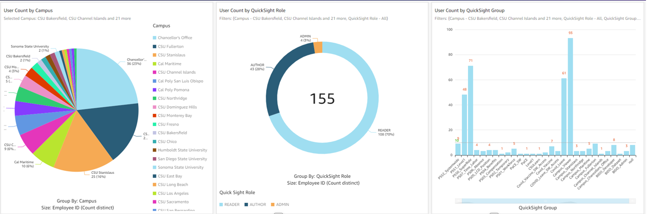
The following screenshot shows an example of the CSUCO security audit dashboard.

Sydnor tells us, “Our previous BI tool had a huge library of visualization, but we don’t need 95% of those. Our presentations look great with the breadth of visuals QuickSight provides. Most people just want the data and ultimately, need a robust vehicle to get data out of a database and onto a table or visualization.”

Converting from their original BI tool to QuickSight was painless for his team. Sydnor tells us that he has “yet to see something we can’t do with QuickSight.” One of Sydnor’s employees who was a user of the previous tool learned QuickSight in just 30 minutes. Now, they conduct QuickSight demos all the time.

Looking to the future: Expanding BI integration and adopting Amazon QuickSight Q

With QuickSight, the Chancellor’s Office aims to roll out more HR dashboards across its campuses and extend the tool for faculty use in the classroom. In the upcoming year, two campuses are joining CSUCO in building their own HR reporting dashboards through QuickSight. The organization is also making plans to use QuickSight to report on student data and implement external-facing dashboards. Some of the data points they’re excited to explore are insights into at-risk students and classroom scheduling on campus.

Thinking ahead, CSUCO is considering Amazon QuickSight Q, a machine learning-powered natural language capability that gives anyone in an organization the ability to ask business questions in natural language and receive accurate answers with relevant visualizations. Sydnor says, “How cool would that be if professors could go in and ask simple, straightforward questions like, ‘How many of my department’s students are taking full course loads this semester?’ It has a lot of potential.”

Summary

The CSUCO is excited to be a champion of QuickSight in the CSU, and are looking for ways to increase its implementation across their organization in the future.

To learn more, visit the website for the California State University Chancellor’s Office. For more on QuickSight, visit the Amazon QuickSight product page, or browse other Big Data Blog posts featuring QuickSight.

About the authors

Madi Hsieh, AWS 2022 Summer Intern, UCLA.

Tina Kelleher, Program Manager at AWS.

Build the next generation, cross-account, event-driven data pipeline orchestration product

2022-11-02 Maria Guerra

Post Syndicated from Maria Guerra original https://aws.amazon.com/blogs/big-data/build-the-next-generation-cross-account-event-driven-data-pipeline-orchestration-product/

This is a guest post by Mehdi Bendriss, Mohamad Shaker, and Arvid Reiche from Scout24.

At Scout24 SE, we love data pipelines, with over 700 pipelines running daily in production, spread across over 100 AWS accounts. As we democratize data and our data platform tooling, each team can create, maintain, and run their own data pipelines in their own AWS account. This freedom and flexibility is required to build scalable organizations. However, it’s full of pitfalls. With no rules in place, chaos is inevitable.

We took a long road to get here. We’ve been developing our own custom data platform since 2015, developing most tools ourselves. Since 2016, we have our self-developed legacy data pipeline orchestration tool.

The motivation to invest a year of work into a new solution was driven by two factors:

Lack of transparency on data lineage, especially dependency and availability of data
Little room to implement governance

As a technical platform, our target user base for our tooling includes data engineers, data analysts, data scientists, and software engineers. We share the vision that anyone with relevant business context and minimal technical skills can create, deploy, and maintain a data pipeline.

In this context, in 2015 we created the predecessor of our new tool, which allows users to describe their pipeline in a YAML file as a list of steps. It worked well for a while, but we faced many problems along the way, notably:

Our product didn’t support pipelines to be triggered by the status of other pipelines, but based on the presence of _SUCCESS files in Amazon Simple Storage Service (Amazon S3). Here we relied on periodic pulls. In complex organizations, data jobs often have strong dependencies to other work streams.
Given the previous point, most pipelines could only be scheduled based on a rough estimate of when their parent pipelines might finish. This led to cascaded failures when the parents failed or didn’t finish on time.
When a pipeline fails and gets fixed, then manually redeployed, all its dependent pipelines must be rerun manually. This means that the data producer bears the responsibility of notifying every single team downstream.

Having data and tooling democratized without the ability to provide insights into which jobs, data, and dependencies exist diminishes synergies within the company, leading to silos and problems in resource allocation. It became clear that we needed a successor for this product that would give more flexibility to the end-user, less computing costs, and no infrastructure management overhead.

In this post, we describe, through a hypothetical case study, the constraints under which the new solution should perform, the end-user experience, and the detailed architecture of the solution.

Case study

Our case study looks at the following teams:

The core-data-availability team has a data pipeline named listings that runs every day at 3:00 AM on the AWS account Account A, and produces on Amazon S3 an aggregate of the listings events published on the platform on the previous day.
The search team has a data pipeline named searches that runs every day at 5:00 AM on the AWS account Account B, and exports to Amazon S3 the list of search events that happened on the previous day.
The rent-journey team wants to measure a metric referred to as X; they create a pipeline named pipeline-X that runs daily on the AWS account Account C, and relies on the data of both previous pipelines. pipeline-X should only run daily, and only after both the listings and searches pipelines succeed.

User experience

We provide users with a CLI tool that we call DataMario (relating to its predecessor DataWario), and which allows users to do the following:

Set up their AWS account with the necessary infrastructure needed to run our solution
Bootstrap and manage their data pipeline projects (creating, deploying, deleting, and so on)

When creating a new project with the CLI, we generate (and require) every project to have a pipeline.yaml file. This file describes the pipeline steps and the way they should be triggered, alerting, type of instances and clusters in which the pipeline will be running, and more.

In addition to the pipeline.yaml file, we allow advanced users with very niche and custom needs to create their pipeline definition entirely using a TypeScript API we provide them, which allows them to use the whole collection of constructs in the AWS Cloud Development Kit (AWS CDK) library.

For the sake of simplicity, we focus on the triggering of pipelines and the alerting in this post, along with the definition of pipelines through pipeline.yaml.

The listings and searches pipelines are triggered as per a scheduling rule, which the team defines in the pipeline.yaml file as follows:

trigger: 
    schedule: 
        hour: 3

pipeline-x is triggered depending on the success of both the listings and searches pipelines. The team defines this dependency relationship in the project’s pipeline.yaml file as follows:

trigger: 
    executions: 
        allOf: 
            - name: listings 
              account: Account_A_ID 
              status: 
                  - SUCCESS 
            - name: searches 
              account: Account_B_ID 
              status: 
                  - SUCCESS

The executions block can define a complex set of relationships by combining the allOf and anyOf blocks, along with a logical operator operator: OR / AND, which allows mixing the allOf and anyOf blocks. We focus on the most basic use case in this post.

Accounts setup

To support alerting, logging, and dependencies management, our solution has components that must be pre-deployed in two types of accounts:

A central AWS account – This is managed by the Data Platform team and contains the following:
- A central data pipeline Amazon EventBridge bus receiving all the run status changes of AWS Step Functions workflows running in user accounts
- An AWS Lambda function logging the Step Functions workflow run changes in an Amazon DynamoDB table to verify if any downstream pipelines should be triggered based on the current event and previous run status changes log
- A Slack alerting service to send alerts to the Slack channels specified by users
- A trigger management service that broadcasts triggering events to the downstream buses in the user accounts
All AWS user accounts using the service – These accounts contain the following:
- A data pipeline EventBridge bus that receives Step Functions workflow run status changes forwarded from the central EventBridge bus
- An S3 bucket to store data pipelines artifacts, along their logs
- Resources needed to run Amazon EMR clusters, like security groups, AWS Identity and Access Management (IAM) roles, and more

With the provided CLI, users can set up their account by running the following code:

$ dpc setup-user-account

Solution overview

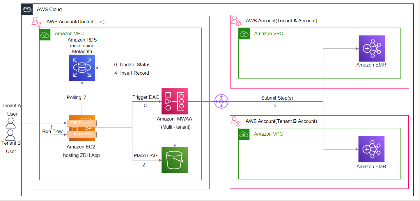
The following diagram illustrates the architecture of the cross-account, event-driven pipeline orchestration product.

In this post, we refer to the different colored and numbered squares to reference a component in the architecture diagram. For example, the green square with label 3 refers to the EventBridge bus default component.

Deployment flow

This section is illustrated with the orange squares in the architecture diagram.

A user can create a project consisting of a data pipeline or more using our CLI tool as follows:

$ dpc create-project -n 'project-name'

The created project contains several components that allow the user to create and deploy data pipelines, which are defined in .yaml files (as explained earlier in the User experience section).

The workflow of deploying a data pipeline such as listings in Account A is as follows:

Deploy listings by running the command dpc deploy in the root folder of the project. An AWS CDK stack with all required resources is automatically generated.
The previous stack is deployed as an AWS CloudFormation template.
The stack uses custom resources to perform some actions, such as storing information needed for alerting and pipeline dependency management.
Two Lambda functions are triggered, one to store the mapping pipeline-X/slack-channels used for alerting in a DynamoDB table, and another one to store the mapping between the deployed pipeline and its triggers (other pipelines that should result in triggering the current one).
To decouple alerting and dependency management services from the other components of the solution, we use Amazon API Gateway for two components:
- The Slack API.
- The dependency management API.
All calls for both APIs are traced in Amazon CloudWatch log groups and two Lambda functions:
- The Slack channel publisher Lambda function, used to store the mapping pipeline_name/slack_channels in a DynamoDB table.
- The dependencies publisher Lambda function, used to store the pipelines dependencies (the mapping pipeline_name/parents) in a DynamoDB table.

Pipeline trigger flow

This is an event-driven mechanism that ensures that data pipelines are triggered as requested by the user, either following a schedule or a list of fulfilled upstream conditions, such as a group of pipelines succeeding or failing.

This flow relies heavily on EventBridge buses and rules, specifically two types of rules:

Scheduling rules.
Step Functions event-based rules, with a payload matching the set of statuses of all the parents of a given pipeline. The rules indicate for which set of statuses all the parents of pipeline-X should be triggered.

Scheduling

This section is illustrated with the black squares in the architecture diagram.

The listings pipeline running on Account A is set to run every day at 3:00 AM. The deployment of this pipeline creates an EventBridge rule and a Step Functions workflow for running the pipeline:

The EventBridge rule is of type schedule and is created on the default bus (this is the EventBridge bus responsible for listening to native AWS events—this distinction is important to avoid confusion when introducing the other buses). This rule has two main components:
- A cron-like notation to describe the frequency at which it runs: 0 3 * * ? *.
- The target, which is the Step Functions workflow describing the workflow of the listings pipeline.
The listings Step Function workflow describes and runs immediately when the rule gets triggered. (The same happens to the searches pipeline.)

Each user account has a default EventBridge bus, which listens to the default AWS events (such as the run of any Lambda function) and scheduled rules.

Dependency management

This section is illustrated with the green squares in the architecture diagram. The current flow starts after the Step Functions workflow (black square 2) starts, as explained in the previous section.

As a reminder, pipeline-X is triggered when both the listings and searches pipelines are successful. We focus on the listings pipeline for this post, but the same applies to the searches pipeline.

The overall idea is to notify all downstream pipelines that depend on it, in every AWS account, passing by and going through the central orchestration account, of the change of status of the listings pipeline.

It’s then logical that the following flow gets triggered multiple times per pipeline (Step Functions workflow) run as its status changes from RUNNING to either SUCCEEDED, FAILED, TIMED_OUT, or ABORTED. The reason being that there could be pipelines downstream potentially listening on any of those status change events. The steps are as follows:

The event of the Step Functions workflow starting is listened to by the default bus of Account A.
The rule export-events-to-central-bus, which specifically listens to the Step Function workflow run status change events, is then triggered.
The rule forwards the event to the central bus on the central account.
The event is then caught by the rule trigger-events-manager.
This rule triggers a Lambda function.
The function gets the list of all children pipelines that depend on the current run status of listings.
The current run is inserted in the run log Amazon Relational Database Service (Amazon RDS) table, following the schema sfn-listings, time (timestamp), status (SUCCEEDED, FAILED, and so on). You can query the run log RDS table to evaluate the running preconditions of all children pipelines and get all those that qualify for triggering.
A triggering event is broadcast in the central bus for each of those eligible children.
Those events get broadcast to all accounts through the export rules—including Account C, which is of interest in our case.
The default EventBridge bus on Account C receives the broadcasted event.
The EventBridge rule gets triggered if the event content matches the expected payload of the rule (notably that both pipelines have a SUCCEEDED status).
If the payload is valid, the rule triggers the Step Functions workflow pipeline-X and triggers the workflow to provision resources (which we discuss later in this post).

Alerting

This section is illustrated with the gray squares in the architecture diagram.

Many teams handle alerting differently across the organization, such as Slack alerting messages, email alerts, and OpsGenie alerts.

We decided to allow users to choose their preferred methods of alerting, giving them the flexibility to choose what kind of alerts to receive:

At the step level – Tracking the entire run of the pipeline
At the pipeline level – When it fails, or when it finishes with a SUCCESS or FAILED status

During the deployment of the pipeline, a new Amazon Simple Notification Service (Amazon SNS) topic gets created with the subscriptions matching the targets specified by the user (URL for OpsGenie, Lambda for Slack or email).

The following code is an example of what it looks like in the user’s pipeline.yaml:

notifications:
    type: FULL_EXECUTION
    targets:
        - channel: SLACK
          addresses:
               - data-pipeline-alerts
        - channel: EMAIL
          addresses:
               - [email protected]

The alerting flow includes the following steps:

As the pipeline (Step Functions workflow) starts (black square 2 in the diagram), the run gets logged into CloudWatch Logs in a log group corresponding to the name of the pipeline (for example, listings).
Depending on the user preference, all the run steps or events may get logged or not thanks to a subscription filter whose target is the execution-tracker-lambda Lambda function. The function gets called anytime a new event gets published in CloudWatch.
This Lambda function parses and formats the message, then publishes it to the SNS topic.
For the email and OpsGenie flows, the flow stops here. For posting the alert message on Slack, the Slack API caller Lambda function gets called with the formatted event payload.
The function then publishes the message to the /messages endpoint of the Slack API Gateway.
The Lambda function behind this endpoint runs, and posts the message in the corresponding Slack channel and under the right Slack thread (if applicable).
The function retrieves the secret Slack REST API key from AWS Secrets Manager.
It retrieves the Slack channels in which the alert should be posted.
It retrieves the root message of the run, if any, so that subsequent messages get posted under the current run thread on Slack.
It posts the message on Slack.
If this is the first message for this run, it stores the mapping with the DB schema execution/slack_message_id to initiate a thread for future messages related to the same run.

Resource provisioning

This section is illustrated with the light blue squares in the architecture diagram.

To run a data pipeline, we need to provision an EMR cluster, which in turn requires some information like Hive metastore credentials, as shown in the workflow. The workflow steps are as follows:

Trigger the Step Functions workflow listings on schedule.
Run the listings workflow.
Provision an EMR cluster.
Use a custom resource to decrypt the Hive metastore password to be used in Spark jobs relying on central Hive tables or views.

End-user experience

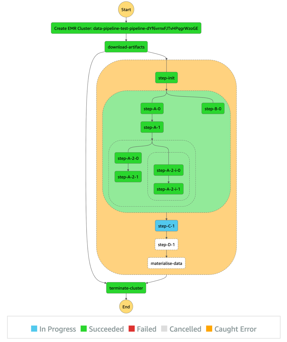
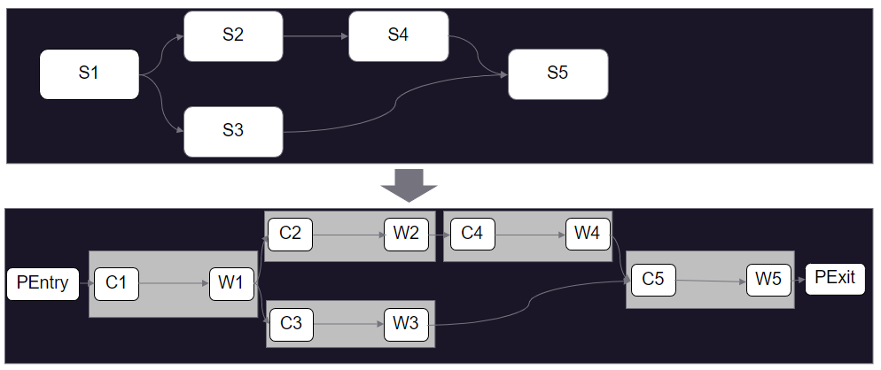
After all preconditions are fulfilled (both the listings and searches pipelines succeeded), the pipeline-X workflow runs as shown in the following diagram.

As shown in the diagram, the pipeline description (as a sequence of steps) defined by the user in the pipeline.yaml is represented by the orange block.

The steps before and after this orange section are automatically generated by our product, so users don’t have to take care of provisioning and freeing compute resources. In short, the CLI tool we provide our users synthesizes the user’s pipeline definition in the pipeline.yaml and generates the corresponding DAG.

Additional considerations and next steps

We tried to stay consistent and stick to one programming language for the creation of this product. We chose TypeScript, which played well with AWS CDK, the infrastructure as code (IaC) framework that we used to build the infrastructure of the product.

Similarly, we chose TypeScript for building the business logic of our Lambda functions, and of the CLI tool (using Oclif) we provide for our users.

As demonstrated in this post, EventBridge is a powerful service for event-driven architectures, and it plays a central and important role in our products. As for its limitations, we found that pairing Lambda and EventBridge could fulfill all our current needs and granted a high level of customization that allowed us to be creative in the features we wanted to serve our users.

Needless to say, we plan to keep developing the product, and have a multitude of ideas, notably:

Extend the list of core resources on which workloads run (currently only Amazon EMR) by adding other compute services, such Amazon Elastic Compute Cloud (Amazon EC2)
Use the Constructs Hub to allow users in the organization to develop custom steps to be used in all data pipelines (we currently only offer Spark and shell steps, which suffice in most cases)
Use the stored metadata regarding pipeline dependencies for data lineage, to have an overview of the overall health of the data pipelines in the organization, and more

Conclusion

This architecture and product brought many benefits. It allows us to:

Have a more robust and clear dependency management of data pipelines at Scout24.
Save on compute costs by avoiding scheduling pipelines based approximately on when its predecessors are usually triggered. By shifting to an event-driven paradigm, no pipeline gets started unless all its prerequisites are fulfilled.
Track our pipelines granularly and in real time on a step level.
Provide more flexible and alternative business logic by exposing multiple event types that downstream pipelines can listen to. For example, a fallback downstream pipeline might be run in case of a parent pipeline failure.
Reduce the cross-team communication overhead in case of failures or stopped runs by increasing the transparency of the whole pipelines’ dependency landscape.
Avoid manually restarting pipelines after an upstream pipeline is fixed.
Have an overview of all jobs that run.
Support the creation of a performance culture characterized by accountability.

We have big plans for this product. We will use DataMario to implement granular data lineage, observability, and governance. It’s a key piece of infrastructure in our strategy to scale data engineering and analytics at Scout24.

We will make DataMario open source towards the end of 2022. This is in line with our strategy to promote our approach to a solution on a self-built, scalable data platform. And with our next steps, we hope to extend this list of benefits and ease the pain in other companies solving similar challenges.

Thank you for reading.

About the authors

Mehdi Bendriss is a Senior Data / Data Platform Engineer, MSc in Computer Science and over 9 years of experience in software, ML, and data and data platform engineering, designing and building large-scale data and data platform products.

Mohamad Shaker is a Senior Data / Data Platform Engineer, with over 9 years of experience in software and data engineering, designing and building large-scale data and data platform products that enable users to access, explore, and utilize their data to build great data products.

Arvid Reiche is a Data Platform Leader, with over 9 years of experience in data, building a data platform that scales and serves the needs of the users.

Marco Salazar is a Solutions Architect working with Digital Native customers in the DACH region with over 5 years of experience building and delivering end-to-end, high-impact, cloud native solutions on AWS for Enterprise and Sports customers across EMEA. He currently focuses on enabling customers to define technology strategies on AWS for the short- and long-term that allow them achieve their desired business objectives, specializing on Data and Analytics engagements. In his free time, Marco enjoys building side-projects involving mobile/web apps, microcontrollers & IoT, and most recently wearable technologies.

Building highly resilient applications with on-premises interdependencies using AWS Local Zones

2022-10-27 Sheila Busser

Post Syndicated from Sheila Busser original https://aws.amazon.com/blogs/compute/building-highly-resilient-applications-with-on-premises-interdependencies-using-aws-local-zones/

This blog post is written by Rachel Rui Liu, Senior Solutions Architect.

AWS Local Zones are a type of infrastructure deployment that places compute, storage, database, and other select AWS services close to large population and industry centers.

Following the successful launch of the AWS Local Zone s in 16 US cities since 2019, in Feb 2022, AWS announced plans to launch new AWS Local Zones in 32 metropolitan areas in 26 countries worldwide.

With Local Zones, we’ve seen use cases in two common categories.

The first category of use cases is for workloads that require extremely low latency between end-user devices and workload servers. For example, let’s consider media content creation and real-time multiplayer gaming. For these use cases, deploying the workload to a Local Zone can help achieve down to single-digit milliseconds latency between end-user devices and the AWS infrastructure, which is ideal for a good end-user experience.

This post will focus on addressing the second category of use cases, which is commonly seen in an enterprise hybrid architecture, where customers must achieve low latency between AWS infrastructure and existing on-premises data centers. Compared to the first category of use cases, these use cases can tolerate slightly higher latency between the end-user devices and the AWS infrastructure. However, these workloads have dependencies to these on-premises systems, so the lowest possible latency between AWS infrastructure and on-premises data centers is required for better application performance. Here are a few examples of these systems:

Financial services sector mainframe workloads hosted on premises serving regional customers.
Enterprise Active Directory hosted on premise serving cloud and on-premises workloads.
Enterprise applications hosted on premises processing a high volume of locally generated data.

For workloads deployed in AWS, the time taken for each interaction with components still hosted in the on-premises data center is increased by the latency. In turn, this delays responses received by the end-user. The total latency accumulates and results in suboptimal user experiences.

By deploying modernized workloads in Local Zones, you can reduce latency while continuing to access systems hosted in on-premises data centers, thereby reducing the total latency for the end-user. At the same time, you can enjoy the benefits of agility, elasticity, and security offered by AWS, and can apply the same automation, compliance, and security best practices that you’ve been familiar with in the AWS Regions.

Enterprise workload resiliency with Local Zones

While designing hybrid architectures with Local Zones, resiliency is an important consideration. You want to route traffic to the nearest Local Zone for low latency. However, when disasters happen, it’s critical to fail over to the parent Region automatically.

Let’s look at the details of hybrid architecture design based on real world deployments from different angles to understand how the architecture achieves all of the design goals.

Hybrid architecture with resilient network connectivity

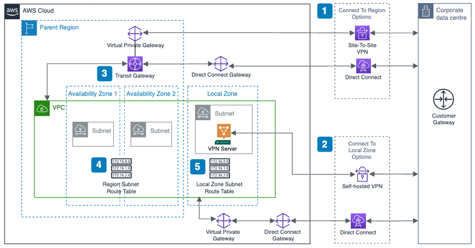
The following diagram shows a high-level overview of a resilient enterprise hybrid architecture with Local Zones, where you have redundant connections between the AWS Region, the Local Zone, and the corporate data center.

Here are a few key points with this network connectivity design:

Use AWS Direct Connect or Site-to-Site VPN to connect the corporate data center and AWS Region.
Use Direct Connect or self-hosted VPN to connect the corporate data center and the Local Zone. This connection will provide dedicated low-latency connectivity between the Local Zone and corporate data center.
Transit Gateway is a regional service. When attaching the VPC to AWS Transit Gateway, you can only add subnets provisioned in the Region. Instances on subnets in the Local Zone can still use Transit Gateway to reach resources in the Region.
For subnets provisioned in the Region, the VPC route table should be configured to route the traffic to the corporate data center via Transit Gateway.
For subnets provisioned in Local Zone, the VPC route table should be configured to route the traffic to the corporate data center via the self-hosted VPN instance or Direct Connect.

Hybrid architecture with resilient workload deployment

The next examples show a public and a private facing workload.

To simplify the diagram and focus on application layer architecture, the following diagrams assume that you are using Direct Connect to connect between AWS and the on-premises data center.

Example 1: Resilient public facing workload

With a public facing workload, end-user traffic will be routed to the Local Zone. If the Local Zone is unavailable, then the traffic will be routed to the Region automatically using an Amazon Route 53 failover policy.

Here are the key design considerations for this architecture:

Deploy the workload in the Local Zone and put the compute layer in an AWS AutoScaling Group, so that the application can scale up and down depending on volume of requests.
Deploy the workload in both the Local Zone and an AWS Region, and put the compute layer into an autoscaling group. The regional deployment will act as pilot light or warm standby with minimal footprint. But it can scale out when the Local Zone is unavailable.
Two Application Load Balancers (ALBs) are required: one in the Region and one in the Local Zone. Each ALB will dispatch the traffic to each workload cluster inside the autoscaling group local to it.
An internet gateway is required for public facing workloads. When using a Local Zone, there’s no extra configuration needed: define a single internet gateway and attach it to the VPC.

If you want to specify an Elastic IP address to be the workload’s public endpoint, the Local Zone will have a different address pool than the Region. Noting that BYOIP is unsupported for Local Zones.

Create a Route 53 DNS record with “Failover” as the routing policy.

For the primary record, point it to the alias of the ALB in the Local Zone. This will set Local Zone as the preferred destination for the application traffic which minimizes latency for end-users.
For the secondary record, point it to the alias of the ALB in the AWS Region.
Enable health check for the primary record. If health check against the primary record fails, which indicates that the workload deployed in the Local Zone has failed to respond, then Route 53 will automatically point to the secondary record, which is the workload deployed in the AWS Region.

Example 2: Resilient private workload

For a private workload that’s only accessible by internal users, a few extra considerations must be made to keep the traffic inside of the trusted private network.

The architecture for resilient private facing workload has the same steps as public facing workload, but with some key differences. These include:

Instead of using a public hosted zone, create private hosted zones in Route 53 to respond to DNS queries for the workload.
Create the primary and secondary records in Route 53 just like the public workload but referencing the private ALBs.
To allow end-users onto the corporate network (within offices or connected via VPN) to resolve the workload, use the Route 53 Resolver with an inbound endpoint. This allows end-users located on-premises to resolve the records in the private hosted zone. Route 53 Resolver is designed to be integrated with an on-premises DNS server.
No internet gateway is required for hosting the private workload. You might need an internet gateway in the Local Zone for other purposes: for example, to host a self-managed VPN solution to connect the Local Zone with the corporate data center.

Hosting multiple workloads

Customers who host multiple workloads in a single VPC generally must consider how to segregate those workloads. As with workloads in the AWS Region, segregation can be implemented at a subnet or VPC level.

If you want to segregate workloads at the subnet level, you can extend your existing VPC architecture by provisioning extra sets of subnets to the Local Zone.

Although not shown in the diagram, for those of you using a self-hosted VPN to connect the Local Zone with an on-premises data center, the VPN solution can be deployed in a centralized subnet.

You can continue to use security groups, network access control lists (NACLs) , and VPC route tables – just as you would in the Region to segregate the workloads.

If you want to segregate workloads at the VPC level, like many of our customers do, within the Region, inter-VPC routing is generally handled by Transit Gateway. However, in this case, it may be undesirable to send traffic to the Region to reach a subnet in another VPC that is also extended to the Local Zone.

Key considerations for this design are as follows:

Direct Connect is deployed to connect the Local Zone with the corporate data center. Therefore, each VPC will have a dedicated Virtual Private Gateway provisioned to allow association with the Direct Connect Gateway.
To enable inter-VPC traffic within the Local Zone, peer the two VPCs together.
Create a VPC route table in VPC A. Add a route for Subnet Y where the destination is the peering link. Assign this route table to Subnet X.
Create a VPC route table in VPC B. Add a route for Subnet X where the destination is the peering link. Assign this route table to Subnet Y.
If necessary, add routes for on-premises networks and the transit gateway to both route tables.

This design allows traffic between subnets X and Y to stay within the Local Zone, thereby avoiding any latency from the Local Zone to the AWS Region while still permitting full connectivity to all other networks.

Conclusion

In this post, we summarized the use cases for enterprise hybrid architecture with Local Zones, and showed you:

Reference architectures to host workloads in Local Zones with low-latency connectivity to corporate data centers and resiliency to enable fail over to the AWS Region automatically.
Different design considerations for public and private facing workloads utilizing this hybrid architecture.
Segregation and connectivity considerations when extending this hybrid architecture to host multiple workloads.

Hopefully you will be able to follow along with these reference architectures to build and run highly resilient applications with local system interdependencies using Local Zones.

How The Mill Adventure enabled data-driven decision-making in iGaming using Amazon QuickSight

2022-10-26 Deepak Singh

Post Syndicated from Deepak Singh original https://aws.amazon.com/blogs/big-data/how-the-mill-adventure-enabled-data-driven-decision-making-in-igaming-using-amazon-quicksight/

This post is co-written with Darren Demicoli from The Mill Adventure.

The Mill Adventure is an iGaming industry enabler offering customizable turnkey solutions to B2B partners and custom branding enablement for its B2C partners. They provide a complete gaming platform, including licenses and operations, for rapid deployment and success in iGaming, and are committed to improving the iGaming experience by being a differentiator through innovation. The Mill Adventure already provides its services to a number of iGaming brands and seeks to continuously grow through the ranks of the industry.

In this post, we show how The Mill Adventure is helping its partners answer business-critical iGaming questions by building a data analytics application using modern data strategy using AWS. This modern data strategy approach has led to high velocity innovation while lowering the total operating cost.

With a gross market revenue exceeding $70 billion and a global player base of around 3 billion players (per a recent imarc Market Overview 2022-2027), the iGaming industry has, without a doubt, been booming over the past few years. This presents a lucrative opportunity to an ever-growing list of businesses seeking to tap into the market and attract a bigger share as their audience. Needless to say, staying competitive in this somewhat saturated market is extremely challenging. Making data-driven decisions is critical to the growth and success of iGaming businesses.

Business challenges

Gaming companies typically generate a massive amount of data, which could potentially enable meaningful insights and answer business-critical questions. Some of the critical and common business challenges in iGaming industry are:

What impacts the brand’s turnover—its new players, retained players, or a mix of both?
How to assess the effectiveness of a marketing campaign? Should a campaign be reinstated? Which games to promote via campaigns?
Which affiliates drive quality players that have better conversion rates? Which paid traffic channels should be discontinued?
For how long does the typical player stay active within a brand? What is the lifetime deposit from a player?
How to improve the registration to first deposit processes? What are the most pressing issues impacting player conversion?

Though sufficient data was captured, The Mill Adventure found two key challenges in their ability to generate actionable insights:

Lack of analysis-ready datasets (not raw and unusable data formats)
Lack of timely access to business-critical data

For example, The Mill Adventure generates over 50 GB of data daily. Its partners have access to this data. However, due to the data being in a raw form, they find it of little value in answering their business-critical questions. This affects their decision-making processes.

To address these challenges, The Mill Adventure chose to build a modern data platform on AWS that was not only capable of providing timely and meaningful business insights for the iGaming industry, but also efficiently manageable, low-cost, scalable, and secure.

Modern data architecture

The Mill Adventure wanted to build a data analytics platform using a modern data strategy that would grow as the company grows. Key tenets of this modern data strategy are:

Build a modern business application and store data in the cloud
Unify data from different application sources into a common data lake, preferably in its native format or in an open file format
Innovate using analytics and machine learning, with an overarching need to meet security and governance compliance requirements

A modern data architecture on AWS applies these tenets. Two key features that form the basic foundation of a modern data architecture on AWS are serverless and microservices.

The Mill Adventure solution

The Mill Adventure built a serverless iGaming data analytics platform that allows its partners to have quick and easy access to a dashboard with data visualizations driven by the varied sources of gaming data, including real-time streaming data. With this platform, stakeholders can use data to devise strategies and plan for future growth based on past performance, evaluate outcomes, and respond to market events with more agility. Having the capability to access insightful information in a timely manner and respond promptly has substantial impact on the turnover and revenue of the business.

A serverless iGaming platform on AWS

In building the iGaming platform, The Mill Adventure was quick to recognize the benefits of having a serverless microservice infrastructure. We wanted to spend time on innovating and building new applications, not managing infrastructure. AWS services such as Amazon API Gateway, AWS Lambda, Amazon DynamoDB, Amazon Kinesis Data Streams, Amazon Simple Storage Service (Amazon S3), Amazon Athena, and Amazon QuickSight are at the core of this data platform solution. Moving to AWS serverless services has saved time, reduced cost, and improved productivity. A microservice architecture has enabled us to accelerate time to value, increase innovation speed, and reduce the need to re-platform, refactor, and rearchitect in the future.

The following diagram illustrates the data flow from the gaming platform to QuickSight.

The data flow includes the following steps:

As players access the gaming portal, associated business functions such as gaming activity, payment, bonus, accounts management, and session management capture the relevant player actions.
Each business function has a corresponding Lambda-based microservice that handles the ingestion of the data from that business function. For example, the Session service handles player session management. The Payment service handles player funds, including deposits and withdrawals from player wallets. Each microservice stores data locally in DynamoDB and manages the create, read, update, and delete (CRUD) tasks for the data. For event sourcing implementation details, see How The Mill Adventure Implemented Event Sourcing at Scale Using DynamoDB.
Data records resulting from the CRUD outputs are written in real time to Kinesis Data Streams, which forms the primary data source for the analytics dashboards of the platform.
Amazon S3 forms the underlying storage for data in Kinesis Data Streams and forms the internal real-time data lake containing raw data.
The raw data is transformed and optimized through custom-built extract, transform, and load (ETL) pipelines and stored in a different S3 bucket in the data lake.
Both raw and processed data are immediately available for querying via Athena and QuickSight.

Raw data is transformed, optimized, and stored as processed data using an hourly data pipeline to meet analytics and business intelligence needs. The following figure shows an example of record counts and the size of the data being written into Kinesis Data Streams, which eventually needs to be processed from the data lake.

These data pipeline jobs can be broadly classified into six main stages:

Cleanup – Filtering out invalid records
Deduplicate – Removing duplicate data records
Aggregate at various levels – Grouping data at various aggregation levels of interest (such as per player, per session, or per hour or day)
Optimize – Writing files to Amazon S3 in optimized Parquet format
Report – Triggering connectors with updated data (such as updates to affiliate providers and compliance)
Ingest – Triggering an event to ingest data in QuickSight for analytics and visualizations

The output of this data pipeline is two-fold:

A transformed data lake that is designed and optimized for fast query performance
A refreshed view of data for all QuickSight dashboards and analyses

Cultivating a data-driven mindset with QuickSight

The Mill Adventure’s partners access their data securely via QuickSight datasets. These datasets are purposefully curated views on top of the transformed data lake. Each partner can access and visualize their data immediately. With QuickSight, partners can build useful dashboards without having deep technical knowledge or familiarity with the internal structure of the data. This approach significantly reduces the time and effort required and speeds up access to valuable gaming insights for business decision-making.

The Mill Adventure also provides each partner with a set of readily available dashboards. These dashboards are built on the years of experience that The Mill Adventure has in the iGaming industry, cover the most common business intelligence requirements, and jumpstart a data-driven mindset.

In the following sections, we provide a high-level overview of some of The Mill Adventure iGaming dashboard features and how these are used to meet the iGaming business analytics needs.

Key performance indicators

This analysis provides a comprehensive set of iGaming key performance indicators (KPIs) across different functional areas, including but not limited to payment activity (deposits and withdrawals), game activity (bets, gross game wins, return to player) and conversion metrics (active customers, active players, unique depositing customers, newly registered customers, new depositing customers, first-time depositors). These are presented concisely in both a quantitative view and in more visual forms.

In the following example KPI report, we can see how by presenting different iGaming metrics for key periods and lifetime, we can identify the overall performance of the brand.

Affiliates analysis

This analysis presents metrics related to the activity generated by players acquired through affiliates. Affiliates usually account for a large share of the traffic driven to gaming sites, and such a report helps identify the most effective affiliates. It informs performance trends per affiliate and compares across different affiliates. By combining data from multiple sources via QuickSight cross-data source joins, affiliate provider-related data such as earnings and clicks can be presented together with other key gaming platform metrics. By having these metrics broken down by affiliate, we can determine which affiliates contribute the most to the brand, as shown in the following example figure.

Cohort analysis

Cohort analyses track the progression of KPIs (such as average deposits) over a period of time for groups of players after their first deposit day. In the following figure, the average deposits per user (ADPU) is presented for players registering in different quarters within the last 2 years. By moving horizontally along each row on the graph, we can see how the ADPU changes for successive quarters for the same group of players. In the following example, the ADPU decreases substantially, indicating higher player churn.

We can use cohort analyses to calculate the churn rate (rate of players who become inactive). Additionally, by averaging the ADPU figures from this analysis, you can extract the lifetime value (LTV) of the ADPU. This shows the average deposit that can be expected to be deposited by players over their lifetime with the brand.

Player onboarding journey

Player onboarding is not a single-step process. In particular, jurisdictional requirements impose a number of compliance checks that need to be fulfilled along various stages during registration flow. All these, plus other steps along the registration (such as email verification), could pose potential pitfalls for players, leading them to fail to complete registration. Showing these steps in QuickSight funnel visuals helps identify such issues and pinpoint any bottlenecks in such flows, as shown in the following example. Additionally, Sankey visuals are used to monitor player movement across registration steps, identifying steps that need to be optimized.

Campaign outcome analysis

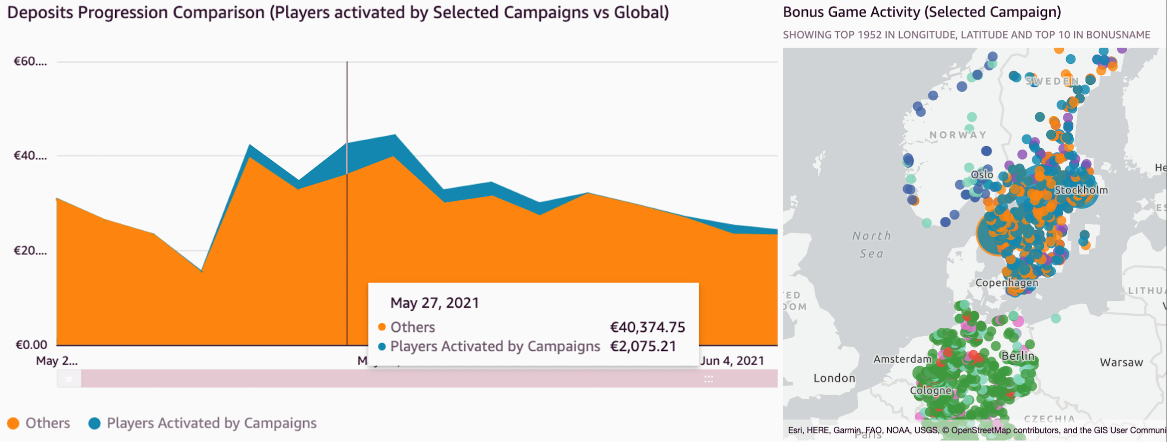
Bonus campaigns are a valuable promotional technique used to reward players and boost engagement. Campaigns can drive turnover and revenue, but there is always an inherent cost associated. It’s critical to assess the performance of campaigns and determine the net outcome. We have built a specific analysis to simplify the task of evaluating these promotions. A number of key metrics related to players activated by campaigns are available. These include both monetary incentives for game activity and deposits and other details related to player demographics (such as country, age group, gender, and channel). Individual campaign performance is analyzed and high-performance ones are identified.

In the following example, the figure on the left shows a time series distribution of deposits coming from campaigns in comparison to the global ones. The figure on the right shows a geographic plot of players activated from selected campaigns.

Demographics distribution analysis

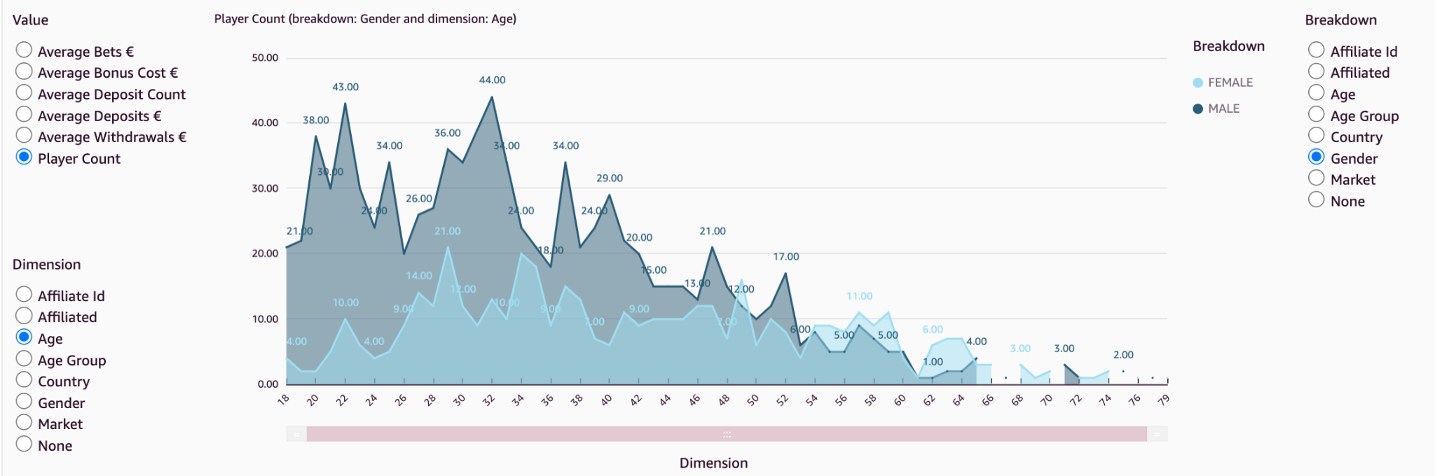
Brands may seek to improve player engagement and retention by tailoring their content for their player base. They need to collect and understand information about their players’ demographics. Players’ demographic distribution varies from brand to brand, and the outcome of actions taken on different brands will vary due to this distribution. Keeping an eye on this demographic (age, country, gender) distribution helps shape a brand strategy in the best way that suits the player base and helps choose the right promotions that appeal most to its audience.

Through visuals such as the following example, it’s possible to quickly analyze the distribution of the selected metric along different demographic categories.

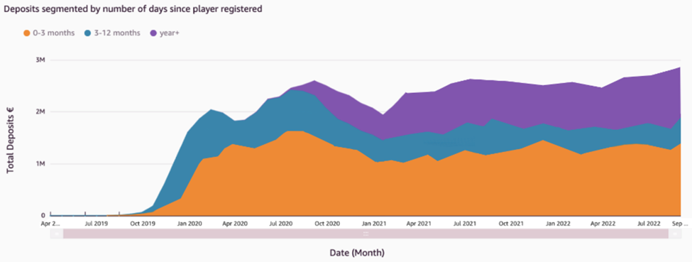
In addition, grouping players by the number of days since registration indicates which players are making a higher contribution to revenue, whether it is existing players or newly registered players. In the following figure, we can see that players who registered in the last 3 months continually account for the highest contribution to deposits. In addition, the proportion of deposits coming from the other two bands of players isn’t increasing, indicating an issue with player retention.

Compliance and responsible gaming

The Mill Adventure treats player protection with the utmost priority. Each iGaming regulated market has its own rules that need to be followed by the gaming operators. These include a number of compliance reports that need to be regularly sent to authorities in the respective jurisdictions. This process was simplified for new brands by creating a common reports template and automating the report creation in QuickSight. This helps new B2B brands meet these reporting requirements quickly and with minimal effort.

In addition, a number of control reports highlighting different areas of player protection are in place. As shown in the following example, responsible gaming reports such as those outlining player behavior deviations help identify accounts with problematic gambling patterns.

Players whose gaming pattern varies from the identified norm are flagged for inspection. This is useful to identify players who may need intervention.

Assessing game play and releases

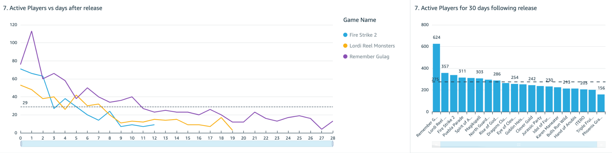
It’s important to measure the performance and popularity of new games post release. Metrics such as unique player participation and player stakes are monitored during the initial days after the release, as shown in the following figures.

Not only does this help evaluate the overall player engagement, but it can also give a clear indication of how these games will perform in the future. By identifying popular games, a brand may choose to focus marketing campaigns on those games, and therefore ensure that it’s promoting games that appeal to its player base.

As shown in these example dashboards, we can use QuickSight to design and create business analytics insights of the iGaming data. This helps us answer real-life business-critical questions and take measurable actions using these insights.

Conclusion

In the iGaming industry, decisions not backed up by data are like an attempt to hit the bullseye blindfolded. With QuickSight, The Mill Adventure empowers its B2B partners and customers to harness data in a timely and convenient manner and support decision-making with winning strategies. Ultimately, in addition to gaining a competitive edge in maximizing revenue opportunities, improved decision-making will also lead to enhanced player experiences.

Reach out to The Mill Adventure and kick-start your iGaming journey today.

Explore rich set of out-of-the-box Amazon QuickSight ML Insights. Amazon QuickSight Q enables dashboards with natural language querying capabilities. For more information and resources on how to get started with free trial, visit Amazon QuickSight.

About the authors

Darren Demicoli is a Senior Devops and Business Intelligence Engineer at The Mill Adventure. He has worked in different roles in technical infrastructure, software development and database administration and has been building solutions for the iGaming sector for the past few years. Outside work, he enjoys travelling, exploring good food and spending time with his family.

Padmaja Suren is a Technical Business Development Manager serving the Public Sector Field Community in Market Intelligence on Analytics. She has 20+ years of experience in building scalable data platforms using a variety of technologies. At AWS she has served as Specialist Solution Architect on services such as Database, Analytics and QuickSight. Prior to AWS, she has implemented successful data and BI initiatives for diverse industry sectors in her capacity as Datawarehouse and BI Architect. She dedicates her free time on her passion project SanghWE which delivers psychosocial education for sexual trauma survivors to heal and recover.

Deepak Singh is a Solution Architect at AWS with specialization in business intelligence and analytics. Deepak has worked across a number of industry verticals such as Finance, Healthcare, Utilities, Retail, and High Tech. Throughout his career, he has focused on solving complex business problems to help customers achieve impactful business outcomes using applied intelligence solutions and services.

How a blockchain startup built a prototype solution to solve the need of analytics for decentralized applications with AWS Data Lab

2022-10-24 Dr. Quan Hoang Nguyen

Post Syndicated from Dr. Quan Hoang Nguyen original https://aws.amazon.com/blogs/big-data/how-a-blockchain-startup-built-a-prototype-solution-to-solve-the-need-of-analytics-for-decentralized-applications-with-aws-data-lab/

This post is co-written with Dr. Quan Hoang Nguyen, CTO at Fantom Foundation.

Here at Fantom Foundation (Fantom), we have developed a high performance, highly scalable, and secure smart contract platform. It’s designed to overcome limitations of the previous generation of blockchain platforms. The Fantom platform is permissionless, decentralized, and open source. The majority of decentralized applications (dApps) hosted on the Fantom platform lack an analytics page that provides information to the users. Therefore, we would like to build a data platform that supports a web interface that will be made public. This will allow users to search for a smart contract address. The application then displays key metrics for that smart contract. Such an analytics platform can give insights and trends for applications deployed on the platform to the users, while the developers can continue to focus on improving their dApps.

AWS Data Lab offers accelerated, joint-engineering engagements between customers and AWS technical resources to create tangible deliverables that accelerate data and analytics modernization initiatives. Data Lab has three offerings: the Build Lab, the Design Lab, and a Resident Architect. The Build Lab is a 2–5 day intensive build with a technical customer team. The Design Lab is a half-day to 2-day engagement for customers who need a real-world architecture recommendation based on AWS expertise, but aren’t yet ready to build. Both engagements are hosted either online or at an in-person AWS Data Lab hub. The Resident Architect provides AWS customers with technical and strategic guidance in refining, implementing, and accelerating their data strategy and solutions over a 6-month engagement.

In this post, we share the experience of our engagement with AWS Data Lab to accelerate the initiative of developing a data pipeline from an idea to a solution. Over 4 weeks, we conducted technical design sessions, reviewed architecture options, and built the proof of concept data pipeline.

Use case review

The process started with us engaging with our AWS Account team to submit a nomination for the data lab. This followed by a call with the AWS Data Lab team to assess the suitability of requirements against the program. After the Build Lab was scheduled, an AWS Data Lab Architect engaged with us to conduct a series of pre-lab calls to finalize the scope, architecture, goals, and success criteria for the lab. The scope was to design a data pipeline that would ingest and store historical and real-time on-chain transactions data, and build a data pipeline to generate key metrics. Once ingested, data should be transformed, stored, and exposed via REST-based APIs and consumed by a web UI to display key metrics. For this Build Lab, we choose to ingest data for Spooky, which is a decentralized exchange (DEX) deployed on the Fantom platform and had the largest Total Value Locked (TVL) at that time. Key metrics such number of wallets that have interacted with the dApp over time, number of tokens and their value exchanged for the dApp over time, and number of transactions for the dApp over time were selected to visualize through a web-based UI.

We explored several architecture options and picked one for the lab that aligned closely with our end goal. The total historical data for the selected smart contract was approximately 1 GB since deployment of dApp on the Fantom platform. We used FTMScan, which allows us to explore and search on the Fantom platform for transactions, to estimate the rate of transfer transactions to be approximately three to four per minute. This allowed us to design an architecture for the lab that can handle this data ingestion rate. We agreed to use an existing application known as the data producer that was developed internally by the Fantom team to ingest on-chain transactions in real time. On checking transactions’ payload size, it was found to not exceed 100 kb for each transaction, which gave us the measure of number of files that will be created once ingested through the data producer application. A decision was made to ingest the past 45 days of historic transactions to populate the platform with enough data to visualize key metrics. Because the feature of backdating exists within the data producer application, we agreed to use that. The Data Lab Architect also advised us to consider using AWS Database Migration Service (AWS DMS) to ingest historic transactions data post lab. As a last step, we decided to build a React-based webpage with Material-UI that allows users to enter a smart contract address and choose the time interval, and the app fetches the necessary data to show the metrics value.

Solution overview

We collectively agreed to incorporate the following design principles for the data lab architecture:

Simplified data pipelines
Decentralized data architecture
Minimize latency as much as possible

The following diagram illustrates the architecture that we built in the lab.

We collectively defined the following success criteria for the Build Lab:

End-to-end data streaming pipeline to ingest on-chain transactions
Historical data ingestion of the selected smart contract
Data storage and processing of on-chain transactions
REST-based APIs to provide time-based metrics for the three defined use cases
A sample web UI to display aggregated metrics for the smart contract

Prior to the Build Lab

As a prerequisite for the lab, we configured the data producer application to use the AWS Software Development Kit (AWS SDK) and PUTRecords API operation to send transactions data to an Amazon Simple Storage Service (Amazon S3) bucket. For the Build Lab, we built additional logic within the application to ingest historic transactions data together with real-time transactions data. As a last step, we verified that transactions data was captured and ingested into a test S3 bucket.

AWS services used in the lab

We used the following AWS services as part of the lab:

AWS Identity and Access Management (IAM) – We created multiple IAM roles with appropriate trust relationships and necessary permissions that can be used by multiple services to read and write on-chain transactions data and generated logs.
Amazon S3 – We created an S3 bucket to store the incoming transactions data as JSON-based files. We created a separate S3 bucket to store incoming transaction data that failed to be transformed and will be reprocessed later.
Amazon Kinesis Data Streams – We created a new Kinesis data stream in on-demand mode, which automatically scales based on data ingestion patterns and provides hands-free capacity management. This stream was used by the data producer application to ingest historical and real-time on-chain transactions. We discussed having the ability to manage and predict cost, and therefore were advised to use the provisioned mode when reliable estimates were available for throughput requirements. We were also advised to continue to use on-demand mode until the data traffic patterns were unpredictable.
Amazon Kinesis Data Firehose – We created a Firehose delivery stream to transform the incoming data and writes it to the S3 bucket. To minimize latency, we set the delivery stream buffer size to 1 MiB and buffer interval to 60 seconds. This would ensure a file is written to the S3 bucket when either of the two conditions are satisfied regardless of the order. Transactions data written to the S3 bucket was in JSON Lines format.
Amazon Simple Queue Service (Amazon SQS) – We set up an SQS queue of the type Standard and an access policy for that SQS queue to allow incoming messages generated from S3 bucket event notifications.
Amazon DynamoDB – In order to pick a data store for on-chain transactions, we needed a service that can store transactions payload of unstructured data with varying schemas, provides the ability to cache query results, and is a managed service. We picked DynamoDB for those reasons. We created a single DynamoDB table that holds the incoming transactions data. After analyzing the access query patterns, we decided to use the address field of the smart contract as the partition key and the timestamp field as the sort key. The table was created with auto scaling of read and write capacity modes because the actual usage requirements would be hard to predict at that time.
AWS Lambda – We created the following functions:
- A Python-based Lambda function to perform transformations on the incoming data from the data producer application to flatten the JSON structure, convert the Unix-based epoch timestamp to a date/time value, and convert hex-based string values to a decimal value representing the number of tokens.
- A second Lambda function to parse incoming SQS queue messages. This message contained values for bucket_name and object_key, which holds the reference to a newly created object within the S3 bucket. The Lambda function logic included parsing of this value to obtain the reference to the S3 object, get the contents of the object, read it into a data frame object using the AWS SDK for pandas (awswrangler) library, convert it into a Pandas data frame object, and use the put_df API call to write a Pandas data frame object as an item into a DynamoDB table. We choose to use Pandas due to familiarity with the library and functions required to perform data transform operations.
- Three separate Lambda functions that contains the logic to query the DynamoDB table and retrieve items to aggregate and calculate metrics values. This calculated metrics value within the Lambda function was formatted as an HTTP response to expose as REST-based APIs.
Amazon API Gateway – We created a REST based API endpoint that uses Lambda proxy integration to pass a smart contract address and time-based interval in minutes as a query string parameter to the backend Lambda function. The response from the Lambda function was a metrics value. We also enabled cross-origin resource sharing (CORS) support within API Gateway to successfully query from the web UI that resides in a different domain.
Amazon CloudWatch – We used a Lambda function in-built mechanism to send function metrics to CloudWatch. Lambda functions come with a CloudWatch Logs log group and a log stream for each instance of your function. The Lambda runtime environment sends details of each invocation to the log stream, and relays logs and other output from your function’s code.

Iterative development approach

Across 4 days of the Build Lab, we undertook iterative development. We started by developing the foundational layer and iteratively added extra features through testing and data validation. This allowed us to develop confidence of the solution being built as we tested the output of the metrics through a web-based UI and verified with the actual data. As errors got discovered, we deleted the entire dataset and reran all the jobs to verify results and resolve those errors.

Lab outcomes

In 4 days, we built an end-to-end streaming pipeline ingesting 45 days of historical data and real-time on-chain transactions data for the selected Spooky smart contract. We also developed three REST-based APIs for the selected metrics and a sample web UI that allows users to insert a smart contract address, choose a time frequency, and visualize the metrics values. In a follow-up call, our AWS Data Lab Architect shared post-lab guidance around the next steps required to productionize the solution:

Scaling of the proof of concept to handle larger data volumes
Security best practices to protect the data while at rest and in transit
Best practices for data modeling and storage
Building an automated resilience technique to handle failed processing of the transactions data
Incorporating high availability and disaster recovery solutions to handle incoming data requests, including adding of the caching layer

Conclusion

Through a short engagement and small team, we accelerated this project from an idea to a solution. This experience gave us the opportunity to explore AWS services and their analytical capabilities in-depth. As a next step, we will continue to take advantage of AWS teams to enhance the solution built during this lab to make it ready for the production deployment.

Learn more about how the AWS Data Lab can help your data and analytics on the cloud journey.

About the Authors

Dr. Quan Hoang Nguyen is currently a CTO at Fantom Foundation. His interests include DLT, blockchain technologies, visual analytics, compiler optimization, and transactional memory. He has experience in R&D at the University of Sydney, IBM, Capital Markets CRC, Smarts – NASDAQ, and National ICT Australia (NICTA).

Ankit Patira is a Data Lab Architect at AWS based in Melbourne, Australia.

Automate Amazon Redshift Serverless data warehouse management using AWS CloudFormation and the AWS CLI

2022-10-19 Ranjan Burman

Post Syndicated from Ranjan Burman original https://aws.amazon.com/blogs/big-data/automate-amazon-redshift-serverless-data-warehouse-management-using-aws-cloudformation-and-the-aws-cli/

Amazon Redshift Serverless makes it simple to run and scale analytics without having to manage the instance type, instance size, lifecycle management, pausing, resuming, and so on. It automatically provisions and intelligently scales data warehouse compute capacity to deliver fast performance for even the most demanding and unpredictable workloads, and you pay only for what you use. Just load your data and start querying right away in the Amazon Redshift Query Editor or in your favorite business intelligence (BI) tool and continue to enjoy the best price performance and familiar SQL features in an easy-to-use, zero administration environment.

Redshift Serverless separates compute and storage and introduces two abstractions:

Workgroup – A workgroup is a collection of compute resources. It groups together compute resources like RPUs, VPC subnet groups, and security groups.
Namespace – A namespace is a collection of database objects and users. It groups together data objects, such as databases, schemas, tables, users, or AWS Key Management Service (AWS KMS) keys for encrypting data.

Some organizations want to automate the creation of workgroups and namespaces for automated infrastructure management and consistent configuration across environments, and provide end-to-end self-service capabilities. You can automate the workgroup and namespace management operations using the Redshift Serverless API, the AWS Command Line Interface (AWS CLI), or AWS CloudFormation, which we demonstrate in this post.

Solution overview

In the following sections, we discuss the automation approaches for various tasks involved in Redshift Serverless data warehouse management using AWS CloudFormation (for more information, see RedshiftServerless resource type reference) and the AWS CLI (see redshift-serverless).

The following are some of the key use cases and appropriate automation approaches to use with AWS CloudFormation:

Enable end-to-end self-service from infrastructure setup to querying
Automate data consumer onboarding for data provisioned through AWS Data Exchange
Accelerate workload isolation by creating endpoints
Create a new data warehouse with consistent configuration across environments

The following are some of the main use cases and approaches for the AWS CLI:

Automate maintenance operations:
- Backup and limits
- Modify RPU configurations
- Manage limits
Automate migration from provisioned to serverless

Prerequisites

To run the operations described in this post, make sure that this user or role has AWS Identity Access and Management (IAM) arn:aws:iam::aws:policy/AWSCloudFormationFullAccess, and either the administrator permission arn:aws:iam::aws:policy/AdministratorAccess or the full Amazon Redshift permission arn:aws:iam::aws:policy/AmazonRedshiftFullAccess policy attached. Refer to Security and connections in Amazon Redshift Serverless for further details.

You should have at least three subnets, and they must span across three Availability Zones.It is not enough if just 3 subnets created in same availability zone. To create a new VPC and subnets, use the following CloudFormation template to deploy in your AWS account.

Create a Redshift Serverless namespace and workgroup using AWS CloudFormation

AWS CloudFormation helps you model and set up your AWS resources so that you can spend less time on infrastructure setup and more time focusing on your applications that run in AWS. You create a template that describes all the AWS resources that you want, and AWS CloudFormation takes care of provisioning and configuring those resources based on the given input parameters.

To create the namespace and workgroup for a Redshift Serverless data warehouse using AWS CloudFormation, complete the following steps:

Choose Launch Stack to launch AWS CloudFormation in your AWS account with a template:
For Stack name, enter a meaningful name for the stack, for example, rsserverless.
Enter the parameters detailed in the following table.

Parameters	Default	Allowed Values	Description
Namespace	.	N/A	The name of the namespace of your choice to be created.
Database Name	dev	N/A	The name of the first database in the Redshift Serverless environment.
Admin User Name	admin	N/A	The administrator’s user name for the Redshift Serverless namespace being create.
Admin User Password	.	N/A	The password associated with the admin user.
Associate IAM Role	.	Comma-delimited list of ARNs of IAM roles	Associate an IAM role to your Redshift Serverless namespace (optional).
Log Export List	userlog, connectionlog, useractivitylog	userlog, connectionlog, useractivitylog	Provide comma-separated values from the list. For example, userlog, connectionlog, useractivitylog. If left blank, LogExport is turned off.
Workgroup	.	N/A	The workgroup name of your choice to be created.
Base RPU	128	Minimum value of 32 and maximum value of 512	The base RPU for the Redshift Serverless workgroup.
Publicly accessible	false	true, false	Indicates if the Redshift Serverless instance is publicly accessible.
Subnet Ids	.	N/A	You must have at least three subnets, and they must span across three Availability Zones.
Security Group Id	.	N/A	The list of security group IDs in your VPC.
Enhanced VPC Routing	false	true, false	The value that specifies whether to enable enhanced VPC routing, which forces Redshift Serverless to route traffic through your VPC.

Pass the parameters provided to the AWS::RedshiftServerless::Namespace and AWS::RedshiftServerless::Workgroup resource types:

Resources:
  RedshiftServerlessNamespace:
    Type: 'AWS::RedshiftServerless::Namespace'
    Properties:
      AdminUsername:
        Ref: AdminUsername
      AdminUserPassword:
        Ref: AdminUserPassword
      DbName:
        Ref: DatabaseName
      NamespaceName:
        Ref: NamespaceName
      IamRoles:
        Ref: IAMRole
      LogExports:
        Ref: LogExportsList        
  RedshiftServerlessWorkgroup:
    Type: 'AWS::RedshiftServerless::Workgroup'
    Properties:
      WorkgroupName:
        Ref: WorkgroupName
      NamespaceName:
        Ref: NamespaceName
      BaseCapacity:
        Ref: BaseRPU
      PubliclyAccessible:
        Ref: PubliclyAccessible
      SubnetIds:
        Ref: SubnetId
      SecurityGroupIds:
        Ref: SecurityGroupIds
      EnhancedVpcRouting:
        Ref: EnhancedVpcRouting        
    DependsOn:
      - RedshiftServerlessNamespace

Perform namespace and workgroup management operations using the AWS CLI

The AWS CLI is a unified tool to manage your AWS services. With just one tool to download and configure, you can control multiple AWS services from the command line and automate them through scripts.

To run the Redshift Serverless CLI commands, you need to install the latest version of AWS CLI. For instructions, refer to Installing or updating the latest version of the AWS CLI.

Now you’re ready to complete the following steps:

Use the following command to create a new namespace:

aws redshift-serverless create-namespace \
    --admin-user-password '<password>' \
    --admin-username cfn-blog-admin \
    --db-name cfn-blog-db \
    --namespace-name 'cfn-blog-ns'

The following screenshot shows an example output.

create-namespace

Use the following command to create a new workgroup mapped to the namespace you just created:

aws redshift-serverless create-workgroup \
    --base-capacity 128 \
    --namespace-name 'cfn-blog-ns' \
    --no-publicly-accessible \
    --security-group-ids "sg-0269bd680e0911ce7" \
    --subnet-ids "subnet-078eedbdd99398568" "subnet-05defe25a59c0e4c2" "subnet-0f378d07e02da3e48"\
    --workgroup-name 'cfn-blog-wg'

The following is an example output.

create workgroup

To allow instances and devices outside the VPC to connect to the workgroup, use the publicly-accessible option in the create-workgroup CLI command.

To verify the workgroup has been created and is in AVAILABLE status, use the following command:

aws redshift-serverless get-workgroup \
--workgroup-name 'cfn-blog-wg' \
--output text \
--query 'workgroup.status'

The following screenshot shows our output.

Regardless of whether your snapshot was made from a provisioned cluster or serverless workgroup, it can be restored into a new serverless workgroup. Restoring a snapshot replaces the namespace and workgroup with the contents of the snapshot.

Use the following command to restore from a snapshot:

aws redshift-serverless restore-from-snapshot \
--namespace-name 'cfn-blog-ns' \
--snapshot-arn arn:aws:redshift:us-east-1:<account-id>:snapshot:<cluster-identifier>/<snapshot-identifier> \
--workgroup-name 'cfn-blog-wg'

The following is an example output.

To check the workgroup status, run the following command:

aws redshift-serverless get-workgroup \
--workgroup-name 'cfn-blog-wg' \
--output text \
--query 'workgroup.status'

To create a snapshot from an existing namespace, run the following command:

aws redshift-serverless create-snapshot \
--namespace-name cfn-blog-ns \
--snapshot-name cfn-blog-snapshot-from-ns \
--retention-period 7

The following is an example output.

Redshift Serverless creates recovery points of your namespace that are available for 24 hours. To keep your recovery point longer than 24 hours, convert it to a snapshot.

To find the recovery points associated to your namespace, run the following command:

aws redshift-serverless list-recovery-points \
--namespace-name cfn-blog-ns \
--no-paginate

The following an example output with the list of all the recovery points.

list recovery points

Let’s take the latest recoveryPointId from the list and convert to snapshot.

To create a snapshot from a recovery point, run the following command:

aws redshift-serverless convert-recovery-point-to-snapshot \
--recovery-point-id f9eaf9ac-a98d-4809-9eee-869ef03e98b4 \
--retention-period 7 \
--snapshot-name cfn-blog-snapshot-from-rp

The following is an example output.

convert-recovery-point

In addition to restoring a snapshot to a serverless namespace, you can also restore from a recovery point.

First, you need to find the recovery point identifier using the list-recovery-points command.
Then use the following command to restore from a recovery point:

aws redshift-serverless restore-from-recovery-point \
--namespace-name cfn-blog-ns \
--recovery-point-id 15c55fb4-d973-4d8a-a8fe-4741e7911137 \
--workgroup-name cfn-blog-wg

The following is an example output.

restore from recovery point

The base RPU determines the starting capacity for your serverless environment.

Use the following command to modify the base RPU based on your workload requirements:

aws redshift-serverless update-workgroup \
--base-capacity 256 \
--workgroup-name 'cfn-blog-wg'

The following is an example output.

Run the following command to verify the workgroup base RPU capacity has been modified to 256:

aws redshift-serverless get-workgroup \
--workgroup-name 'cfn-blog-wg' \
--output text \
--query 'workgroup.baseCapacity'

To keep costs predictable for Redshift Serverless, you can set the maximum RPU hours used per day, per week, or per month. In addition, you can take action when the limit is reached. Actions include: write a log entry to a system table, receive an alert, or turn off user queries.

Use the following command to first get the workgroup ARN:

aws redshift-serverless get-workgroup --workgroup-name 'cfn-blog-wg' \
--output text \
--query 'workgroup.workgroupArn'

The following screenshot shows our output.

Use the workgroupArn output from the preceding command with the following command to set the daily RPU usage limit and set the action behavior to log:

aws redshift-serverless create-usage-limit \
--amount 256 \
--breach-action log \
--period daily \
--resource-arn arn:aws:redshift-serverless:us-east-1:<aws-account-id>:workgroup/1dcdd402-8aeb-432e-8833-b1f78a112a93 \
--usage-type serverless-compute

The following is an example output.

Conclusion

You have now learned how to automate management operations on Redshift Serverless namespaces and workgroups using AWS CloudFormation and the AWS CLI. To automate creation and management of Amazon Redshift provisioned clusters, refer to Automate Amazon Redshift Cluster management operations using AWS CloudFormation.

About the Authors

Ranjan Burman is a Analytics Specialist Solutions Architect at AWS. He specializes in Amazon Redshift and helps customers build scalable analytical solutions. He has more than 15 years of experience in different database and data warehousing technologies. He is passionate about automating and solving customer problems with the use of cloud solutions.

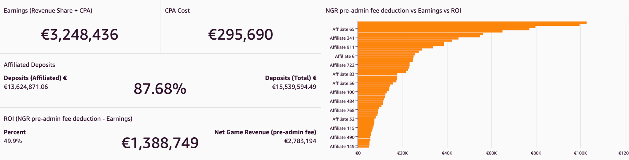
Satesh Sonti is a Sr. Analytics Specialist Solutions Architect based out of Atlanta, specialized in building enterprise data platforms, data warehousing, and analytics solutions. He has over 16 years of experience in building data assets and leading complex data platform programs for banking and insurance clients across the globe.

Urvish Shah is a Senior Database Engineer at Amazon Redshift. He has more than a decade of experience working on databases, data warehousing and in analytics space. Outside of work, he enjoys cooking, travelling and spending time with his daughter.

Adding approval notifications to EC2 Image Builder before sharing AMIs

2022-10-14 Sheila Busser

Post Syndicated from Sheila Busser original https://aws.amazon.com/blogs/compute/adding-approval-notifications-to-ec2-image-builder-before-sharing-amis-2/

This blog post is written by, Glenn Chia Jin Wee, Associate Cloud Architect, and Randall Han, Professional Services.

You may be required to manually validate the Amazon Machine Image (AMI) built from an Amazon Elastic Compute Cloud (Amazon EC2) Image Builder pipeline before sharing this AMI to other AWS accounts or to an AWS organization. Currently, Image Builder provides an end-to-end pipeline that automatically shares AMIs after they’ve been built.

In this post, we will walk through the steps to enable approval notifications before AMIs are shared with other AWS accounts. Image Builder supports automated image testing using test components. The recommended best practice is to automate test steps, however situations can arise where test steps become either challenging to automate or internal compliance policies mandate manual checks be conducted prior to distributing images. In such situations, having a manual approval step is useful if you would like to verify the AMI configuration before it is shared to other AWS accounts or an AWS Organization. A manual approval step reduces the potential for sharing an incorrectly configured AMI with other teams which can lead to downstream issues. This solution sends an email with a link to approve or reject the AMI. Users approve the AMI after they’ve verified that it is built according to specifications. Upon approving the AMI, the solution automatically shares it with the specified AWS accounts.

Overview

In this solution, an Image Builder Pipeline is run that builds a Golden AMI in Account A. After the AMI is built, Image Builder publishes data about the AMI to an Amazon Simple Notification Service (Amazon SNS)
The SNS Topic passes the data to an AWS Lambda function that subscribes to it.
The Lambda function that subscribes to this topic retrieves the data, formats it, and then starts an SSM Automation, passing it the AMI Name and ID.
The first step of the SSM Automation is a manual approval step. The SSM Automation first publishes to an SNS Topic that has an email subscription with the Approver’s email. The approver will receive the email with a URL that they can click to approve the step.
The approval step defines a specific AWS Identity and Access Management (IAM) Role as an approver. This role has the minimum required permissions to approve the manual approval step. After performing manual tests on the Golden AMI, the Approver principal will assume this role.
After assuming this role, the approver will click on the approval link that was sent via email. After approving the step, an AWS Lambda Function is triggered.
This Lambda Function shares the Golden AMI with Account B and sends an email notifying the Target Account Recipients that the AMI has been shared.

Prerequisites

For this walkthrough, you will need the following:

Two AWS accounts – one to host the solution resources, and the second which receives the shared Golden AMI.
- In the account that hosts the solution, prepare an AWS Identity and Access Management (IAM) principal with the sts:AssumeRole permission. This principal must assume the IAM Role that is listed as an approver in the Systems Manager approval step. The ARN of this IAM principal is used in the AWS CloudFormation Approver parameter, This ARN is added to the trust policy of approval IAM Role.
- In addition, in the account hosting the solution, ensure that the IAM principal deploying the CloudFormation template has the required permissions to create the resources in the stack.
A new Amazon Virtual Private Cloud (Amazon VPC) will be created from the stack. Make sure that you have fewer than five VPCs in the selected Region.

Walkthrough

In this section, we will guide you through the steps required to deploy the Image Builder solution. The solution is deployed with CloudFormation.

In this scenario, we deploy the solution within the approver’s account. The approval email will be sent to a predefined email address for manual approval, before the newly created AMI is shared to target accounts.

The approver first assumes the approval IAM Role and then selects the approval link. This leads to the Systems Manager approval page. Upon approval, an email notification will be sent to the predefined target account email address, notifying the relevant stakeholders that the AMI has been successfully shared.

The high-level steps we will follow are:

In Account A, deploy the provided AWS CloudFormation template. This includes an example Image Builder Pipeline, Amazon SNS topics, Lambda functions, and an SSM Automation Document.
Approve the SNS subscription from your supplied email address.
Run the pipeline from the Amazon EC2 Image Builder Console.
[Optional] To conduct manual tests, launch an Amazon EC2 instance from the built AMI after the pipeline runs.
An email will be sent to you with options to approve or reject the step. Ensure that you have assumed the IAM Role that is the approver before clicking the approval link that leads to the SSM console approval page.
Upon approving the step, an AWS Lambda function shares the AMI to the Account B and also sends an email to the target account email recipients notifying them that the AMI has been shared.
Log in to Account B and verify that the AMI has been shared.

Step 1: Deploy the AWS CloudFormation template

1. The CloudFormation template, template.yaml that deploys the solution can also found at this GitHub repository. Follow the instructions at the repository to deploy the stack.

Step 2: Verify your email address

After running the deployment, you will receive an email prompting you to confirm the Subscription at the approver email address. Choose Confirm subscription.

This leads to the following screen, which shows that your subscription is confirmed.

Repeat the previous 2 steps for the target email address.

Step 3: Run the pipeline from the Image Builder console

In the Image Builder console, under Image pipelines, select the checkbox next to the Pipeline created, choose Actions, and select Run pipeline.

Note: The pipeline takes approximately 20 – 30 minutes to complete.

Step 4: [Optional] Launch an Amazon EC2 instance from the built AMI

If you have a requirement to manually validate the AMI before sharing it with other accounts or to the AWS organization an approver will launch an Amazon EC2 instance from the built AMI and conduct manual tests on the EC2 instance to make sure it is functional.

In the Amazon EC2 console, under Images, choose AMIs. Validate that the AMI is created.

Follow AWS docs: Launching an EC2 instances from a custom AMI for steps on how to launch an Amazon EC2 instance from the AMI.

Step 5: Select the approval URL in the email sent

When the pipeline is run successfully, you will receive another email with a URL to approve the AMI.

Before clicking on the Approve link, you must assume the IAM Role that is set as an approver for the Systems Manager step.
In the CloudFormation console, choose the stack that was deployed.

4. Choose Outputs and copy the IAM Role name.

5. While logged in as the IAM Principal that has permissions to assume the approval IAM Role, follow the instructions at AWS IAM documentation for switching a role using the console to assume the approval role.
In the Switch Role page, in Role paste the name of the IAM Role that you copied in the previous step.

Note: This IAM Role was deployed with minimum permissions. Hence, seeing warning messages in the console is expected after assuming this role.

6. Now in the approval email, select the Approve URL. This leads to the Systems Manager console. Choose Submit.

7. After approving the manual step, the second step is executed, which shares the AMI to the target account.

Step 6: Verify that the AMI is shared to Account B

Log in to Account B.
In the Amazon EC2 console, under Images, choose AMIs. Then, in the dropdown, choose Private images. Validate that the AMI is shared.

Verify that a success email notification was sent to the target account email address provided.

Clean up

This section provides the necessary information for deleting various resources created as part of this post.

Deregister the AMIs that were created and shared.
1. Log in to Account A and follow the steps at AWS documentation: Deregister your Linux AMI.
Delete the CloudFormation stack. For instructions, refer to Deleting a stack on the AWS CloudFormation console.

Conclusion

In this post, we explained how to enable approval notifications for an Image Builder pipeline before AMIs are shared to other accounts. This solution can be extended to share to more than one AWS account or even to an AWS organization. With this solution, you will be notified when new golden images are created, allowing you to verify the accuracy of their configuration before sharing them to for wider use. This reduces the possibility of sharing AMIs with misconfigurations that the written tests may not have identified.

We invite you to experiment with different AMIs created using Image Builder, and with different Image Builder components. Check out this GitHub repository for various examples that use Image Builder. Also check out this blog on Image builder integrations with EC2 Auto Scaling Instance Refresh. Let us know your questions and findings in the comments, and have fun!

Fine-tuning Operations at Slice using AWS DevOps Guru

2022-10-12 Adnan Bilwani

Post Syndicated from Adnan Bilwani original https://aws.amazon.com/blogs/devops/fine-tuning-operations-at-slice-using-aws-devops-guru/

This guest post was authored by Sapan Jain, DevOps Engineer at Slice, and edited by Sobhan Archakam and Adnan Bilwani, at AWS.

Slice empowers over 18,000 independent pizzerias with the modern tools that have grown the major restaurant chains. By uniting these small businesses with specialized technology, marketing, data insights, and shared services, Slice enables them to serve their digitally-minded customers and move away from third-party apps. Using Amazon DevOps Guru, Slice is able to fine-tune their operations to better support these customers.

Serial tech entrepreneur Ilir Sela started Slice to modernize and support his family’s New York City pizzerias. Today, the company partners with restaurants in 3,000 cities and all 50 states, forming the nation’s largest pizza network. For more information, visit slicelife.com.

Slice’s challenge

At Slice, we manage a wide variety of systems, services, and platforms, all with varying levels of complexity. Observability, monitoring, and log aggregation are things we excel at, and they’re always critical for our platform engineering team. However, deriving insights from this data still requires some manual investigation, particularly when dealing with operational anomalies and/or misconfigurations.

To gain automated insights into our services and resources, Slice conducted a proof-of-concept utilizing Amazon DevOps Guru to analyze a small selection of AWS resources. Amazon DevOps Guru identified potential issues in our environment, resulting in actionable insights (ultimately leading to remediation). As a result of this analysis, we enabled Amazon DevOps Guru account-wide, thereby leading to numerous insights into our production environment.

Insights with Amazon DevOps Guru

After we configured Amazon DevOps Guru to begin its account-wide analysis, we left the tool alone to begin the process of collecting and analyzing data. We immediately began seeing some actionable insights for various production AWS resources, some of which are highlighted in the following section:

Amazon DynamoDB Point-in-time recovery

Amazon DynamoDB offers a point-in-time recovery (PITR) feature that provides continuous backups of your DynamoDB data for 35 days to help you protect against accidental write or deletes. If enabled, this lets you restore your respective table to a previous state. Amazon DevOps Guru identified several tables in our environment that had PITR disabled, along with a corresponding Recommendation.

The graphic shows proactive insights for the last 1 month. The one insight shown is 'Dynamo Table Point in Time Recovery not enabled' with a status of OnGoing and a severity of low.

Figure 1. The graphic shows proactive insights for the last 1 month. The one insight shown is ‘Dynamo Table Point in Time Recovery not enabled’ with a status of OnGoing and a severity of low.

Elasticache anomalous evictions

Amazon Elasticache for Redis is used by a handful of our services to cache any relevant application data. Amazon DevOps Guru identified that one of our instances was exhibiting anomalous behavior regarding its cache eviction rate. Essentially, due to the memory pressure of the instance, the eviction rate of cache entries began to increase. DevOps Guru recommended revisiting the sizing of this instance and scaling it vertically or horizontally, where appropriate.

The graph shows the metric: count of ElastiCache evictions plotted for the time period Jul 3, 20:35 to Jul 3, 21:35 UTC. A highlighted section shows that the evictions increased to a peak of 2500 between 21:00 and 21:08. Outside of this interval the evictions are below 500.

Figure 2. The graph shows the metric: count of ElastiCache evictions plotted for the time period Jul 3, 20:35 to Jul 3, 21:35 UTC. A highlighted section shows that the evictions increased to a peak of 2500 between 21:00 and 21:08. Outside of this interval the evictions are below 500

AWS Lambda anomalous errors

We manage a few AWS Lambda functions that all serve different purposes. During the beginning of normal work day, we began to see increased error rates for a particular function resulting in an exception being thrown. DevOps Guru was able to detect the increase in error rates and flag them as anomalous. Although retries in this case wouldn’t have solved the problem, it did increase our visibility into the issue (which was also corroborated by our APM platform).

The graph shows the metric: count of AWS/Lambda errors plotted between 11:00 and 13:30 on Jul 6. The sections between the times 11:23 and 12:15 and at 12:37 and 13:13 UTC are highlighted to show the anomalies.

Figure 3. The graph shows the metric: count of AWS/Lambda errors plotted between 11:00 and 13:30 on Jul 6. The sections between the times 11:23 and 12:15 and at 12:37 and 13:13 UTC are highlighted to show the anomalies

Figure 3. The graph shows the metric: count of AWS/Lambda errors plotted between 11:00 and 13:30 on Jul 6. The sections between the times 11:23 and 12:15 UTC are highlighted to show the anomalies

Conclusion

Amazon DevOps Guru integrated into our environment quickly, with no more additional configuration or setup aside from a few button clicks to enable the service. After reviewing several of the proactive insights that DevOps Guru provided, we could formulate plans of action regarding remediation. One specific case example of this is where DevOps Guru flagged several of our Lambda functions for not containing enough subnets. After triaging the finding, we discovered that we were lacking multi-AZ redundancy for several of those functions. As a result, we could implement a change that maximized our availability of those resources.

With the continuous analysis that DevOps Guru performs, we continue to gain new insights into the resources that we utilize and deploy in our environment. This lets us improve operationally while simultaneously maintaining production stability.

About the author:

Best Practices for Hosting Regulated Gaming Workloads in AWS Local Zones and on AWS Outposts

2022-10-07 Sheila Busser

Post Syndicated from Sheila Busser original https://aws.amazon.com/blogs/compute/best-practices-for-hosting-regulated-gaming-workloads-in-aws-local-zones-and-on-aws-outposts/

This blog post is written by Shiv Bhatt, Manthan Raval, and Pawan Matta, who are Senior Solutions Architects with AWS.

Many industries are subject to regulations that are created to protect the interests of the various stakeholders. For some industries, the specific details of the regulatory requirements influence not only the organization’s operations, but also their decisions for adopting new technology. In this post, we highlight the workload residency challenges that you may encounter when you deploy regulated gaming workloads, and how AWS Local Zones and AWS Outposts can help you address those challenges.

Regulated gaming workloads and residency requirements

A regulated gaming workload is a type of workload that’s subject to federal, state, local, or tribal laws related to the regulation of gambling and real money gaming. Examples of these workloads include sports betting, horse racing, casino, poker, lottery, bingo, and fantasy sports. The operators provide gamers with access to these workloads through online and land-based channels, and they’re required to follow various regulations required in their jurisdiction. Some regulations define specific workload residency requirements, and depending on the regulatory agency, the regulations could require that workloads be hosted within a specific city, state, province, or country. For example, in the United States, different state and tribal regulatory agencies dictate whether and where gaming operations are legal in a state, and who can operate. The agencies grant licenses to the operators of regulated gaming workloads, which then govern who can operate within the state, and sometimes, specifically where these workloads can be hosted. In addition, federal legislation can also constrain how regulated gaming workloads can be operated. For example, the United States Federal Wire Act makes it illegal to facilitate bets or wagers on sporting events across state lines. This regulation requires that operators make sure that users who place bets in a specific state are also within the borders of that state.

Benefits of using AWS edge infrastructure with regulated gaming workloads

The use of AWS edge infrastructure, specifically Local Zones and Outposts to host a regulated gaming workload, can help you meet workload residency requirements. You can manage Local Zones and Outposts by using the AWS Management Console or by using control plane API operations, which lets you seamlessly consume compute, storage, and other AWS services.

Local Zones

Local Zones are a type of AWS infrastructure deployment that place compute, storage, database, and other select services closer to large population, industry, and IT centers. Like AWS Regions, Local Zones enable you to innovate more quickly and bring new products to market sooner without having to worry about hardware and data center space procurement, capacity planning, and other forms of undifferentiated heavy-lifting. Local Zones have their own connections to the internet, and support AWS Direct Connect, so that workloads hosted in the Local Zone can serve local end-users with very low-latency communications. Local Zones are by default connected to a parent Region via Amazon’s redundant and high-bandwidth private network. This lets you extend Amazon Virtual Private Cloud (Amazon VPC) in the AWS Region to Local Zones. Furthermore, this provides applications hosted in AWS Local Zones with fast, secure, and seamless access to the broader portfolio of AWS services in the AWS Region. You can see the full list of AWS services supported in Local Zones on the AWS Local Zones features page.

You can start using Local Zones right away by enabling them in your AWS account. There are no setup fees, and as with the AWS Region, you pay only for the services that you use. There are three ways to pay for Amazon Elastic Compute Cloud (Amazon EC2) instances in Local Zones: On-Demand, Savings Plans, and Spot Instances. See the full list of cities where Local Zones are available on the Local Zones locations page.

Outposts

Outposts is a family of fully-managed solutions that deliver AWS infrastructure and services to most customer data center locations for a consistent hybrid experience. For a full list of countries and territories where Outposts is available, see the Outposts rack FAQs and Outposts servers FAQs. Outposts is available in various form factors, from 1U and 2U Outposts servers to 42U Outposts racks, and multiple rack deployments. To learn more about specific configuration options and pricing, see Outposts rack and Outposts servers.

You configure Outposts to work with a specific AWS Region using AWS Direct Connect or an internet connection, which lets you extend Amazon VPC in the AWS Region to Outposts. Like Local Zones, this provides applications hosted on Outposts with fast, secure, and seamless access to the broader portfolio of AWS services in the AWS Region. See the full list of AWS services supported on Outposts rack and on Outposts servers.

Choosing between AWS Regions, Local Zones, and Outposts

When you build and deploy a regulated gaming workload, you must assess the residency requirements carefully to make sure that your workload complies with regulations. As you make your assessment, we recommend that you consider separating your regulated gaming workload into regulated and non-regulated components. For example, for a sports betting workload, the regulated components might include sportsbook operation, and account and wallet management, while non-regulated components might include marketing, the odds engine, and responsible gaming. In describing the following scenarios, it’s assumed that regulated and non-regulated components must be fault-tolerant.

For hosting the non-regulated components of your regulated gaming workload, we recommend that you consider using an AWS Region instead of a Local Zone or Outpost. An AWS Region offers higher availability, larger scale, and a broader selection of AWS services.

For hosting regulated components, the type of AWS infrastructure that you choose will depend on which of the following scenarios applies to your situation:

Scenario one: An AWS Region is available in your jurisdiction and local regulators have approved the use of cloud services for your regulated gaming workload.
Scenario two: An AWS Region isn’t available in your jurisdiction, but a Local Zone is available, and local regulators have approved the use of cloud services for your regulated gaming workload.
Scenario three: An AWS Region or Local Zone isn’t available in your jurisdiction, or local regulators haven’t approved the use of cloud services for your regulated gaming workload, but Outposts is available.

Let’s look at each of these scenarios in detail.

Scenario one: Use an AWS Region for regulated components

When local regulators have approved the use of cloud services for regulated gaming workloads, and an AWS Region is available in your jurisdiction, consider using an AWS Region rather than a Local Zone and Outpost. For example, in the United States, the State of Ohio has announced that it will permit regulated gaming workloads to be deployed in the cloud on infrastructure located within the state when sports betting goes live in January 2023. By using the US East (Ohio) Region, operators in the state don’t need to procure and manage physical infrastructure and data center space. Instead, they can use various compute, storage, database, analytics, and artificial intelligence/machine learning (AI/ML) services that are readily available in the AWS Region. You can host a regulated gaming workload entirely in a single AWS Region, which includes Availability Zones (AZs) – multiple, isolated locations within each AWS Region. By deploying your workload redundantly across at least two AZs, you can help make sure of the high availability, as shown in the following figure.

Scenario two: Use a Local Zone for regulated components

A second scenario might be that local regulators have approved the use of cloud services for regulated gaming workloads, and an AWS Region isn’t available in your jurisdiction, but a Local Zone is available. In this scenario, consider using a Local Zone rather than Outposts. A Local Zone can support more elasticity in a more cost-effective way than Outposts can. However, you might also consider using a Local Zone and Outposts together to increase availability and scalability for regulated components. Let’s consider the State of Illinois, in the United States, which allows regulated gaming workloads to be deployed in the cloud, if workload residency requirements are met. Operators in this state can host regulated components in a Local Zone in Chicago, and they can also use Outposts in their data center in the same state, for high availability and disaster recovery, as shown in the following figure.

Scenario three: Use of Outposts for regulated components

When local regulators haven’t approved the use of cloud services for regulated gaming workloads, or when an AWS Region or Local Zone isn’t available in your jurisdiction, you can still choose to host your regulated gaming workloads on Outposts for a consistent cloud experience, if Outposts is available in your jurisdiction. If you choose to use Outposts, then note that as part of the shared responsibility model, customers are responsible for attesting to physical security and access controls around the Outpost, as well as environmental requirements for the facility, networking, and power. Use of Outposts requires you to procure and manage the data center within the city, state, province, or country boundary (as required by local regulations) that may be suitable to host regulated components, depending on the jurisdiction. Furthermore, you should procure and configure supported network connections between Outposts and the parent AWS Region. During the Outposts ordering process, you should account for the compute and network capacity required to support the peak load and availability design.

For a higher availability level, you should consider procuring and deploying two or more Outposts racks or Outposts servers in a data center. You might also consider deploying redundant network paths between Outposts and the parent AWS Region. However, depending on your business service level agreement (SLA) for regulated gaming workload, you might choose to spread Outposts racks across two or more isolated data centers within the same regulated boundary, as shown in the following figure.

Options to route ingress gaming traffic

You have two options to route ingress gaming traffic coming into your regulated and non-regulated components when you deploy the configurations that we described previously in Scenarios two and three. Your gaming traffic can come through to the AWS Region, or through the Local Zones or Outposts. Note that the benefits that we mentioned previously around selecting the AWS Region for deploying regulated and non-regulated components are the same when you select an ingress route.

Let’s discuss the benefits and trade offs for each of these options.

Option one: Route ingress gaming traffic through an AWS Region

If you choose to route ingress gaming traffic through an AWS Region, your regulated gaming workloads benefit from access to the wide range of tools, services, and capacity available in the AWS Region. For example, native AWS security services, like AWS WAF and AWS Shield, which provide protection against DDoS attacks, are currently only available in AWS Regions. Only traffic that you route into your workload through an AWS Region benefits from these services.

If you route gaming traffic through an AWS Region, and non-regulated components are hosted in an AWS Region, then traffic has a direct path to non-regulated components. In addition, gaming traffic destined to regulated components, hosted in a Local Zone and on Outposts, can be routed through your non-regulated components and a few native AWS services in the AWS Region, as shown in Figure 2.

Option two: Route ingress gaming traffic through a Local Zone or Outposts

Choosing to route ingress gaming traffic through a Local Zone or Outposts requires careful planning to make sure that tools, services, and capacity are available in that jurisdiction, as shown in the following figure. In addition, consider how choosing this route will influence the pillars of the AWS Well-Architected Framework. This route might require deploying and managing most of your non-regulated components in a Local Zone or on Outposts as well, including native AWS services that aren’t available in Local Zones or on Outposts. If you plan to implement this topology, then we recommend that you consider using AWS Partner solutions to replace the native AWS services that aren’t available in Local Zones or Outposts.

Conclusion

If you’re building regulated gaming workloads, then you might have to follow strict workload residency and availability requirements. In this post, we’ve highlighted how Local Zones and Outposts can help you meet these workload residency requirements by bringing AWS services closer to where they’re needed. We also discussed the benefits of using AWS Regions in compliment to the AWS edge infrastructure, and several reliability and cost design considerations.

Although this post provides information to consider when making choices about using AWS for regulated gaming workloads, you’re ultimately responsible for maintaining compliance with the gaming regulations and laws in your jurisdiction. You’re in the best position to determine and maintain ultimate responsibility for determining whether activities are legal, including evaluating the jurisdiction of the activities, how activities are made available, and whether specific technologies or services are required to make sure of compliance with the applicable law. You should always review these regulations and laws before you deploy regulated gaming workloads on AWS.

Automate data archival for Amazon Redshift time series tables

2022-10-04 Nita Shah

Post Syndicated from Nita Shah original https://aws.amazon.com/blogs/big-data/automate-data-archival-for-amazon-redshift-time-series-tables/

Amazon Redshift is a fast, scalable, secure, and fully managed cloud data warehouse that makes it simple and cost-effective to analyze all of your data using standard SQL. Tens of thousands of customers today rely on Amazon Redshift to analyze exabytes of data and run complex analytical queries, making it the most widely used cloud data warehouse. You can run and scale analytics in seconds on all your data without having to manage your data warehouse infrastructure.

A data retention policy is part of an organization’s overall data management. In a big data world, the size of data is consistently increasing, which directly affects the cost of storing the data in data stores. It’s necessary to keep optimizing your data in data warehouses for consistent performance, reliability, and cost control. It’s crucial to define how long an organization needs to hold on to specific data, and if data that is no longer needed should be archived or deleted. The frequency of data archival depends on the relevance of the data with respect to your business or legal needs.

Data archiving is the process of moving data that is no longer actively used in a data warehouse to a separate storage device for long-term retention. Archive data consists of older data that is still important to the organization and may be needed for future reference, as well as data that must be retained for regulatory compliance.

Data purging is the process of freeing up space in the database or deleting obsolete data that isn’t required by the business. The purging process can be based on the data retention policy, which is defined by the data owner or business need.

This post walks you through the process of how to automate data archival and purging of Amazon Redshift time series tables. Time series tables retain data for a certain period of time (days, months, quarters, or years) and need data to be purged regularly to maintain the rolling data to be analyzed by end-users.

Solution overview

The following diagram illustrates our solution architecture.

We use two database tables as part of this solution.

The arch_table_metadata database table stores the metadata for all the tables that need to be archived and purged. You need to add rows into this table that you want to archive and purge. The arch_table_metadata table contains the following columns.

ColumnName	Description
`id`	Database-generated, automatically assigns a unique value to each record.
`schema_name`	Name of the database schema of the table.
`table_name`	Name of the table to be archived and purged.
`column_name`	Name of the date column that is used to identify records to be archived and purged.
`s3_uri`	Amazon S3 location where the data will be archived.
`retention_days`	Number of days the data will be retained for the table. Default is 90 days.

The arch_job_log database table stores the run history of stored procedures. Records are added to this table by the stored procedure. It contains the following columns.

ColumnName	Description
`job_run_id`	Assigns unique numeric value per stored procedure run.
`arch_table_metadata_id`	Id column value from table `arch_table_metadata`.
`no_of_rows_bfr_delete`	Number of rows in the table before purging.
`no_of_rows_deleted`	Number of rows deleted by the purge operation.
`job_start_time`	Time in UTC when the stored procedure started.
`job_end_time`	Time in UTC when the stored procedure ended.
`job_status`	Status of the stored procedure run: IN-PROGRESS, COMPLETED, or FAILED.

Prerequisites

For this solution, complete the following prerequisites:

Create an Amazon Redshift provisioned cluster or Amazon Redshift serverless workgroup.

In Amazon Redshift query editor v2 or a compatible SQL editor of your choice, create the tables arch_table_metadata and arch_job_log. Use the following code for the table DDLs:

create table arch_table_metadata
(
id integer identity(0,1) not null, 
schema_name varchar(100) not null, 
table_name varchar(100) not null, 
column_name varchar(100) not null,
s3_uri varchar(1000) not null,
retention_days integer default 90
);

create table arch_job_log
(
job_run_id bigint not null, 
arch_table_metadata_id  integer not null,
no_of_rows_bfr_delete bigint,
no_of_rows_deleted bigint,
table_arch_start_time timestamp default current_timestamp,
table_arch_end_time timestamp default current_timestamp,
job_start_time timestamp default current_timestamp,
job_end_time timestamp default current_timestamp,
job_status varchar(20)
);

Create the stored procedure sp_archive_data with the following code snippet. The stored procedure takes the AWS Identity and Access Management (IAM) role ARN as an input argument if you’re not using the default IAM role. If you’re using the default IAM role for your Amazon Redshift cluster, you can pass the input parameter as default. For more information, refer to Creating an IAM role as default in Amazon Redshift.

CREATE OR REPLACE PROCEDURE archive_data_sp(p_iam_role IN varchar(256))
AS $$
DECLARE

v_command           varchar(500);
v_sql               varchar(500);
v_count_sql         text;

v_table_id          int;
v_schema_name       text;
v_table_name        text;
v_column_name       text;
v_s3_bucket_url     text;
v_s3_folder_name_prefix     text;
v_retention_days            int = 0;
v_no_of_rows_before_delete  int = 0;
v_no_of_deleted_rows        int =0;
v_job_start_time            timestamp;
v_job_status                int = 1;
v_job_id                    int =0;


table_meta_data_cur CURSOR FOR
SELECT id, schema_name, table_name, column_name,s3_uri,retention_days
FROM arch_table_metadata;

BEGIN

    SELECT NVL(MAX(job_run_id),0) + 1 INTO v_job_id FROM arch_job_log;
    RAISE NOTICE '%', v_job_id;

    OPEN table_meta_data_cur;
    FETCH table_meta_data_cur INTO v_table_id,v_schema_name, v_table_name, v_column_name, v_s3_bucket_url, v_retention_days;
    WHILE v_table_id IS NOT NULL LOOP

        v_count_sql = 'SELECT COUNT(*) AS v_no_of_rows_before_delete FROM ' || v_schema_name || '.' || v_table_name;
        RAISE NOTICE '%', v_count_sql;
        EXECUTE v_count_sql INTO v_no_of_rows_before_delete;
        RAISE NOTICE 'v_no_of_rows_before_delete %', v_no_of_rows_before_delete;

        v_job_start_time = GETDATE();
        v_s3_folder_name_prefix = v_schema_name || '.' || v_table_name || '/';
        v_sql = 'SELECT * FROM ' || v_schema_name || '.' || v_table_name || ' WHERE ' || v_column_name || ' <= DATEADD(DAY,-' || v_retention_days || ',CURRENT_DATE)';

        IF p_iam_role = 'default' THEN
            v_command = 'UNLOAD (''' || v_sql ||  ''') to ''' || v_s3_bucket_url || v_s3_folder_name_prefix || ''' IAM_ROLE default  PARQUET PARTITION BY (' || v_column_name || ') INCLUDE ALLOWOVERWRITE';
        ELSE
            v_command = 'UNLOAD (''' || v_sql ||  ''') to ''' || v_s3_bucket_url || v_s3_folder_name_prefix || ''' IAM_ROLE ''' || p_iam_role || ''' PARQUET PARTITION BY (' || v_column_name || ') INCLUDE ALLOWOVERWRITE';
        END IF;
        RAISE NOTICE '%', v_command;
        EXECUTE v_command;

        v_sql := 'DELETE FROM ' || v_schema_name || '.' || v_table_name || ' WHERE ' || v_column_name || ' <= DATEADD(DAY,-' || v_retention_days || ',CURRENT_DATE)';
        RAISE NOTICE '%', v_sql;
        EXECUTE v_sql;

        GET DIAGNOSTICS v_no_of_deleted_rows := ROW_COUNT;
        RAISE INFO '# of rows deleted = %', v_no_of_deleted_rows;

        v_sql = 'INSERT INTO arch_job_log (job_run_id, arch_table_metadata_id ,no_of_rows_bfr_delete,no_of_rows_deleted,job_start_time,job_end_time,job_status) VALUES ('
                    || v_job_id || ',' || v_table_id || ',' || v_no_of_rows_before_delete || ',' || v_no_of_deleted_rows || ',''' || v_job_start_time || ''',''' || GETDATE() || ''',' || v_job_status || ')';
        RAISE NOTICE '%', v_sql;
        EXECUTE v_sql;

        FETCH table_meta_data_cur INTO v_table_id,v_schema_name, v_table_name, v_column_name, v_s3_bucket_url, v_retention_days;
    END LOOP;
    CLOSE table_meta_data_cur;

    EXCEPTION
    WHEN OTHERS THEN
        RAISE NOTICE 'Error - % ', SQLERRM;
END;
$$ LANGUAGE plpgsql;

Archival and purging

For this use case, we use a table called orders, for which we want to archive and purge any records older than the last 30 days.

Use the following DDL to create the table in the Amazon Redshift cluster:

create table orders (
  O_ORDERKEY bigint NOT NULL,
  O_CUSTKEY bigint,
  O_ORDERSTATUS varchar(1),
  O_TOTALPRICE decimal(18,4),
  O_ORDERDATE Date,
  O_ORDERPRIORITY varchar(15),
  O_CLERK varchar(15),
  O_SHIPPRIORITY Integer,
  O_COMMENT varchar(79))
distkey (O_ORDERKEY)
sortkey (O_ORDERDATE);

The O_ORDERDATE column makes it a time series table, which you can use to retain the rolling data for a certain period.

In order to load the data into the orders table using the below COPY command , you would need to have default IAM role attached to your Redshift cluster or replace the default keyword in the COPY command with the arn of the IAM role attached to the Redshift cluster

copy orders from 's3://redshift-immersionday-labs/data/orders/orders.tbl.'
iam_role default
region 'us-west-2' lzop delimiter '|' COMPUPDATE PRESET;

When you query the table, you can see that this data is for 1998. To test this solution, you need to manually update some of the data to the current date by running the following SQL statement:

update orders set O_ORDERDATE = current_date where O_ORDERDATE < '1998-08-02';

The table looks like the following screenshot after running the update statement.

Now let’s run the following SQL to get the count of number of records to be archived and purged:

select count (*) from orders where O_ORDERDATE <= DATEADD(DAY,-30,CURRENT_DATE)

Before running the stored procedure, we need to insert a row into the arch_file_metadata table for the stored procedure to archive and purge records in the orders table. In the following code, provide the Amazon Simple Storage Service (Amazon S3) bucket name where you want to store the archived data:

INSERT INTO arch_table_metadata (schema_name, table_name, column_name, s3_uri, retention_days) VALUES ('public', 'orders', 'O_ORDERDATE', 's3://<your-bucketname>/redshift_data_archival/', 30);

The stored procedure performs the following high-level steps:

Open a cursor to read and loop through the rows in the arch_table_metadata table.
Retrieve the total number of records in the table before purging.
Export and archive the records to be deleted into the Amazon S3 location as specified in the s3_uri column value. Data is partitioned in Amazon S3 based on the column_name field in arch_table_metadata. The stored procedure uses the IAM role passed as input for the UNLOAD operation.
Run the DELETE command to purge the identified records based on the retention_days column value.
Add a record in arch_job_log with the run details.

Now, let’s run the stored procedure via the call statement passing a role ARN as input parameter to verify the data was archived and purged correctly:

call archive_data_sp('arn:aws:iam:<your-account-id>:role/RedshiftRole-7OR1UWVPFI5J');

As shown in the following screenshot, the stored procedure ran successfully.

Now let’s validate the table was purged successfully by running the following SQL:

select count (*) from orders where O_ORDERDATE <= DATEADD(DAY,-30,CURRENT_DATE)

We can navigate to the Amazon S3 location to validate the archival process. The following screenshot shows the data has been archived into the Amazon S3 location specified in the arch_table_metadata table.

Now let’s run the following SQL statement to look at the stored procedure run log entry:

select a.* from arch_job_log a, arch_table_metadata b
where a.arch_table_metadata_id = b.id
and b.table_name = 'orders'

The following screenshot shows the query results.

In this example, we demonstrated how you can set up and validate your Amazon Redshift table archival and purging process.

Schedule the stored procedure

Now that you have learned how to set up and validate your Amazon Redshift tables for archival and purging, you can schedule this process. For instructions on how to schedule a SQL statement using either the AWS Management Console or the AWS Command Line Interface (AWS CLI), refer to Scheduling SQL queries on your Amazon Redshift data warehouse.

Archive data in Amazon S3

As part of this solution, data is archived in an S3 bucket before it’s deleted from the Amazon Redshift table. This helps reduce the storage on the Amazon Redshift cluster and enables you to analyze the data for any ad hoc requests without needing to load back into the cluster. In the stored procedure, the UNLOAD command exports the data to be purged to Amazon S3, partitioned by the date column, which is used to identify the records to purge. To save costs on Amazon S3 storage, you can manage the storage lifecycle with Amazon S3 lifecycle configuration.

Analyze the archived data in Amazon S3 using Amazon Redshift Spectrum

With Amazon Redshift Spectrum, you can efficiently query and retrieve structured and semistructured data from files in Amazon S3, and easily analyze the archived data in Amazon S3 without having to load it back in Amazon Redshift tables. For further analysis of your archived data (cold data) and frequently accessed data (hot data) in the cluster’s local disk, you can run queries joining Amazon S3 archived data with tables that reside on the Amazon Redshift cluster’s local disk. The following diagram illustrates this process.

Let’s take an example where you want to view the number of orders for the last 2 weeks of December 1998, which is archived in Amazon S3. You need to complete the following steps using Redshift Spectrum:

Create an external schema in Amazon Redshift.

Create a late-binding view to refer to the underlying Amazon S3 files with the following query:

create view vw_orders_hist as select count(*),o_orderdate
from <external_schema>. orders 
where o_orderdate between '1998-12-15' and '1998-12-31' group by 2
with no schema binding;

To see a unified view of the orders historical data archived in Amazon S3 and the current data stored in the Amazon Redshift local table, you can use a UNION ALL clause to join the Amazon Redshift orders table and the Redshift Spectrum orders table:
```
create view vw_orders_unified as 
select * from <external_schema>.orders
union all
select * from public.orders
with no schema binding;
```

To learn more about the best practices for Redshift Spectrum, refer to Best Practices for Amazon Redshift Spectrum.

Best practices

The following are some best practices to reduce your storage footprint and optimize performance of your workloads:

Conclusion

In this post, we demonstrated the automatic archival and purging of data in Amazon Redshift tables to meet your compliance and business requirements, thereby optimizing your application performance and reducing storage costs. As an administrator, you can start working with application data owners to identify retention policies for Amazon Redshift tables to achieve optimal performance, prevent any storage issues specifically for DS2 and DC2 nodes, and reduce overall storage costs.

About the authors

Nita Shah is an Analytics Specialist Solutions Architect at AWS based out of New York. She has been building data warehouse solutions for over 20 years and specializes in Amazon Redshift. She is focused on helping customers design and build enterprise-scale well-architected analytics and decision support platforms.

Ranjan Burman is an Analytics Specialist Solutions Architect at AWS. He specializes in Amazon Redshift and helps customers build scalable analytical solutions. He has more than 15 years of experience in different database and data warehousing technologies. He is passionate about automating and solving customer problems with the use of cloud solutions.

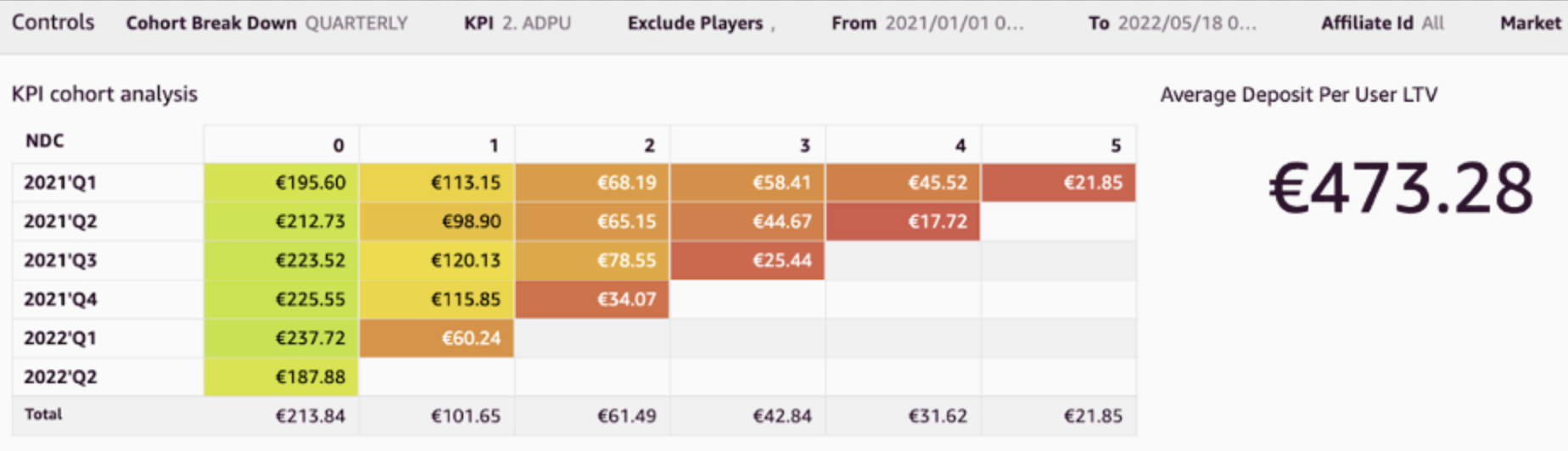
Prathap Thoguru is an Enterprise Solutions Architect at Amazon Web Services. He has over 15 years of experience in the IT industry and is a 9x AWS certified professional. He helps customers migrate their on-premises workloads to the AWS Cloud.

How AWS Data Lab helped BMW Financial Services design and build a multi-account modern data architecture

2022-09-27 Rahul Shaurya

Post Syndicated from Rahul Shaurya original https://aws.amazon.com/blogs/big-data/how-aws-data-lab-helped-bmw-financial-services-design-and-build-a-multi-account-modern-data-architecture/

This post is co-written by Martin Zoellner, Thomas Ehrlich and Veronika Bogusch from BMW Group.

BMW Group and AWS announced a comprehensive strategic collaboration in 2020. The goal of the collaboration is to further accelerate BMW Group’s pace of innovation by placing data and analytics at the center of its decision-making. A key element of the collaboration is the further development of the Cloud Data Hub (CDH) of BMW Group. This is the central platform for managing company-wide data and data solutions in the cloud. At the AWS re:Invent 2019 session, BMW and AWS demonstrated the new Cloud Data Hub platform by outlining different archetypes of data platforms and then walking through the journey of building BMW Group’s Cloud Data Hub. To learn more about the Cloud Data Hub, refer to BMW Cloud Data Hub: A reference implementation of the modern data architecture on AWS.

As part of this collaboration, BMW Group is migrating hundreds of data sources across several data domains to the Cloud Data Hub. Several of these sources pertain to BMW Financial Services.

In this post, we talk about how the AWS Data Lab is helping BMW Financial Services build a regulatory reporting application for one of the European BMW market using the Cloud Data Hub on AWS.

Solution overview

In the context of regulatory reporting, BMW Financial Services works with critical financial services data that contains personally identifiable information (PII). We need to provide monthly insights on our financial data to one of the European National Regulator, and we also need to be compliant with the Schrems II and GDPR regulations as we process PII data. This requires the PII to be pseudonymized when it’s loaded into the Cloud Data Hub, and it has to be processed further in pseudonymized form. For an overview of pseudonymization process, check out Build a pseudonymization service on AWS to protect sensitive data .

To address these requirements in a precise and efficient way, BMW Financial Services decided to engage with the AWS Data Lab. The AWS Data Lab has two offerings: the Design Lab and the Build Lab.

Design Lab

The Design Lab is a 1-to-2-day engagement for customers who need a real-world architecture recommendation based on AWS expertise, but aren’t ready to build. In the case of BMW Financial Services, before beginning the build phase, it was key to get all the stakeholders in the same room and record all the functional and non-functional requirements introduced by all the different parties that might influence the data platform—from owners of the various data sources to end-users that would use the platform to run analytics and get business insights. Within the scope of the Design Lab, we discussed three use cases:

Regulatory reporting – The top priority for BMW Financial Services was the regulatory reporting use case, which involves collecting and calculating data and reports that will be declared to the National Regulator.
Local data warehouse – For this use case, we need to calculate and store all key performance indicators (KPIs) and key value indicators (KVIs) that will be defined during the project. The historical data needs to be stored, but we need to apply a pseudonymization process to respect GDPR directives. Moreover, historical data has to be accessed on a daily basis through a tableau visualization tool. Regarding the structure, it would be valuable to define two levels (at minimum): one at the contract level to justify the calculation of all KPIs, and another at an aggregated level to optimize restitutions. Personal data is limited in the application, but a reidentification process must be possible for authorized consumption patterns.
Accounting details – This use case is based on the BMW accounting tool IFT, which provides the accounting balance at the contract level from all local market applications. It must run at least once a month. However, if some issues are identified on IFT during closing, we must be able to restart it and erase the previous run. When the month-end closing is complete, this use case has to keep the last accounting balance version generated during the month and store it. In parallel, all accounting balance versions have to be accessible by other applications for queries and be able to retrieve the information for 24 months.

Design Lab Solution Architecture

Based on these requirements, we developed the following architecture during the Design Lab.

This solution contains the following components:

The main data source that hydrates our three use cases is the already available in the Cloud Data Hub. The Cloud Data Hub uses AWS Lake Formation resource links to grant access to the dataset to the consumer accounts.
For standard, periodic ETL (extract, transform, and load) jobs that involve operations such as converting data types, or creating labels based on numerical values or Boolean flags based on a label, we used AWS Glue ETL jobs.
For historical ETL jobs or more complex calculations such as in the account details use case, which may involve huge joins with custom configurations and tuning, we recommended to use Amazon EMR. This gives you the opportunity to control cluster configurations at a fine-grained level.
To store job metadata that enables features such as reprocessing inputs or rerunning failed jobs, we recommended building a data registry. The goal of the data registry is to create a centralized inventory for any data being ingested in the data lake. A schedule-based AWS Lambda function could be triggered to register data landing on the semantic layer of the Cloud Data Hub in a centralized metadata store. We recommended using Amazon DynamoDB for the data registry.
Amazon Simple Storage Service (Amazon S3) serves as the storage mechanism that powers the regulatory reporting use case using the data management framework Apache Hudi. Apache Hudi is useful for our use cases because we need to develop data pipelines where record-level insert, update, upsert, and delete capabilities are desirable. Hudi tables are supported by both Amazon EMR and AWS Glue jobs via the Hudi connector, along with query engines such as Amazon Athena and Amazon Redshift Spectrum.
As part of the data storing process in the regulatory reporting S3 bucket, we can populate the AWS Glue Data Catalog with the required metadata.
Athena provides an ad hoc query environment for interactive analysis of data stored in Amazon S3 using standard SQL. It has an out-of-the-box integration with the AWS Glue Data Catalog.
For the data warehousing use case, we need to first de-normalize data to create a dimensional model that enables optimized analytical queries. For that conversion, we use AWS Glue ETL jobs.
Dimensional data marts in Amazon Redshift enable our dashboard and self-service reporting needs. Data in Amazon Redshift is organized into several subject areas that are aligned with the business needs, and a dimensional model allows for cross-subject area analysis.
As a by-product of creating an Amazon Redshift cluster, we can use Redshift Spectrum to access data in the regulatory reporting bucket of the architecture. It acts as a front to access more granular data without actually loading it in the Amazon Redshift cluster.
The data provided to the Cloud Data Hub contains personal data that is pseudonymized. However, we need our pseudonymized columns to be re-personalized when visualizing them on Tableau or when generating CSV reports. Both Athena and Amazon Redshift support Lambda UDFs, which can be used to access Cloud Data Hub PII APIs to re-personalize the pseudonymized columns before presenting them to end-users.
Both Athena and Amazon Redshift can be accessed via JDBC (Java Database Connectivity) to provide access to data consumers.
We can use a Python shell job in AWS Glue to run a query against either of our analytics solutions, convert the results to the required CSV format, and store them to a BMW secured folder.
Any business intelligence (BI) tool deployed on premises can connect to both Athena and Amazon Redshift and use their query engines to perform any heavy computation before it receives the final data to fuel its dashboards.
For the data pipeline orchestration, we recommended using AWS Step Functions because of its low-code development experience and its full integration with all the other components discussed.

With the preceding architecture as our long-term target state, we concluded the Design Lab and decided to return for a Build Lab to accelerate solution development.

Preparing for Build Lab

The typical preparation of a Build Lab that follows a Design Lab involves identifying a few examples of common use case patterns, typically the more complex ones. To maximize the success in the Build Lab, we reduce the long-term target architecture to a subset of components that addresses those examples and can be implemented within a 3-to-5-day intense sprint.

For a successful Build Lab, we also need to identify and resolve any external dependencies, such as network connectivity to data sources and targets. If that isn’t feasible, then we find meaningful ways to mock them. For instance, to make the prototype closer to what the production environment would look like, we decided to use separate AWS accounts for each use case, based on the existing team structure of BMW, and use a consumer S3 bucket instead of BMW network-attached storage (NAS).

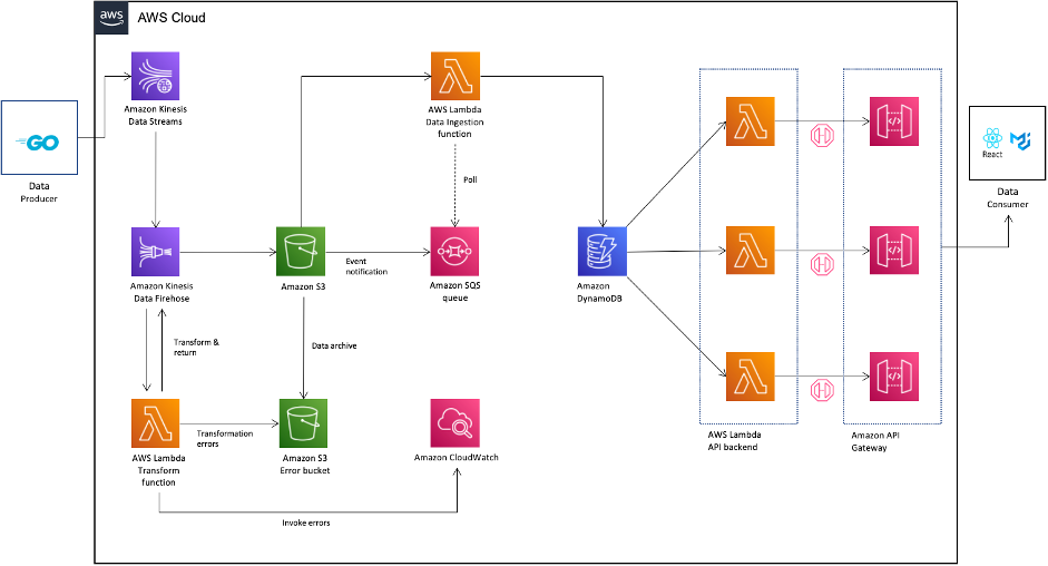
Build Lab

The BMW team set aside 4 days for their Build Lab. During that time, their dedicated Data Lab Architect worked alongside the team, helping them to build the following prototype architecture.

Build Lab Solution

This solution includes the following components:

The first step was to synchronize the AWS Glue Data Catalog of the Cloud Data Hub and regulatory reporting accounts.
AWS Glue jobs running on the regulatory reporting account had access to the data in the Cloud Data Hub resource accounts. During the Build Lab, the BMW team implemented ETL jobs for six tables, addressing insert, update, and delete record requirements using Hudi.
The result of the ETL jobs is stored in the data lake layer stored in the regulatory reporting S3 bucket as Hudi tables that are catalogued in the AWS Glue Data Catalog and can be consumed by multiple AWS services. The bucket is encrypted using AWS Key Management Service (AWS KMS).
Athena is used to run exploratory queries on the data lake.
To demonstrate the cross-account consumption pattern, we created an Amazon Redshift cluster on it, created external tables from the Data Catalog, and used Redshift Spectrum to query the data. To enable cross-account connectivity between the subnet group of the Data Catalog of the regulatory reporting account and the subnet group of the Amazon Redshift cluster on the local data warehouse account, we had to enable VPC peering. To accelerate and optimize the implementation of these configurations during the Build Lab, we received support from an AWS networking subject matter expert, who ran a valuable session, during which the BMW team understood the networking details of the architecture.
For data consumption, the BMW team implemented an AWS Glue Python shell job that connected to Amazon Redshift or Athena using a JDBC connection, ran a query, and stored the results in the reporting bucket as a CSV file, which would later be accessible by the end-users.
End-users can also directly connect to both Athena and Amazon Redshift using a JDBC connection.
We decided to orchestrate the AWS Glue ETL jobs using AWS Glue Workflows. We used the resulting workflow for the end-of-lab demo.

With that, we completed all the goals we had set up and concluded the 4-day Build Lab.

Conclusion

In this post, we walked you through the journey the BMW Financial Services team took with the AWS Data Lab team to participate in a Design Lab to identify a best-fit architecture for their use cases, and the subsequent Build Lab to implement prototypes for regulatory reporting in one of the European BMW market.

To learn more about how AWS Data Lab can help you turn your ideas into solutions, visit AWS Data Lab.

Special thanks to everyone who contributed to the success of the Design and Build Lab: Lionel Mbenda, Mario Robert Tutunea, Marius Abalarus, Maria Dejoie.

About the authors

Martin Zoellner is an IT Specialist at BMW Group. His role in the project is Subject Matter Expert for DevOps and ETL/SW Architecture.

Thomas Ehrlich is the functional maintenance manager of Regulatory Reporting application in one of the European BMW market.

Veronika Bogusch is an IT Specialist at BMW. She initiated the rebuild of the Financial Services Batch Integration Layer via the Cloud Data Hub. The ingested data assets are the base for the Regulatory Reporting use case described in this article.

George Komninos is a solutions architect for the Amazon Web Services (AWS) Data Lab. He helps customers convert their ideas to a production-ready data product. Before AWS, he spent three years at Alexa Information domain as a data engineer. Outside of work, George is a football fan and supports the greatest team in the world, Olympiacos Piraeus.

Rahul Shaurya is a Senior Big Data Architect with AWS Professional Services. He helps and works closely with customers building data platforms and analytical applications on AWS. Outside of work, Rahul loves taking long walks with his dog Barney.

Implementing long running deployments with AWS CloudFormation Custom Resources using AWS Step Functions

2022-09-17 DAMODAR SHENVI WAGLE

Post Syndicated from DAMODAR SHENVI WAGLE original https://aws.amazon.com/blogs/devops/implementing-long-running-deployments-with-aws-cloudformation-custom-resources-using-aws-step-functions/

AWS CloudFormation custom resource provides mechanisms to provision AWS resources that don’t have built-in support from CloudFormation. It lets us write custom provisioning logic for resources that aren’t supported as resource types under CloudFormation. This post focusses on the use cases where CloudFormation custom resource is used to implement a long running task/job. With custom resources, you can manage these custom tasks (which are one-off in nature) as deployment stack resources.

The routine pattern used for implementing custom resources is via AWS Lambda function. However, when using the Lambda function as the custom resource provider, you must consider its trade-offs, such as its 15 minute timeout. Tasks involved in the provisioning of certain AWS resources can be long running and could span beyond the Lambda timeout. In these scenarios, you must look beyond the conventional Lambda function-based approach for custom resources.

In this post, I’ll demonstrate how to use AWS Step Functions to implement custom resources using AWS Cloud Development Kit (AWS CDK). Step Functions allow complex deployment tasks to be orchestrated as a step-by-step workflow. It also offers direct integration with any AWS service via AWS SDK integrations. By default the CloudFormation stack waits for 1 hour before timing out. The timeout can be increased to maximum 12 hours using wait conditions. In this post, you’ll also see how to use wait conditions with custom resource to run long running deployment tasks as part of a CloudFormation stack.

Prerequisites

Before proceeding any further, you must identify and designate an AWS account required for the solution to work. You must also create an AWS account profile in ~/.aws/credentials for the designated AWS account, if you don’t already have one. The profile must have sufficient permissions to run an AWS CDK stack. It should be your private profile and only be used during the course of this post. Therefore, it should be fine if you want to use admin privileges. Don’t share the profile details, especially if it has admin privileges. I recommend removing the profile when you’re finished with this walkthrough. For more information about creating an AWS account profile, see Configuring the AWS CLI.

Services and frameworks used in the post include CloudFormation, Step Functions, Lambda, DynamoDB, Amazon S3, and AWS CDK.

Solution overview

The following architecture diagram shows the application of Step Functions to implement custom resources.

Figure 1. Architecture diagram

The user deploys a CloudFormation stack that includes a custom resource implementation.
The CloudFormation custom resource triggers a Lambda function with the appropriate event which can be CREATE/UPDATE/DELETE.
The custom resource Lambda function invokes Step Functions workflow and offloads the event handling responsibility. The CloudFormation event and context are wrapped inside the Step Function input at the time of invocation.
The custom resource Lambda function returns SUCCESS back to CloudFormation stack indicating that the custom resource provisioning has begun. CloudFormation stack then goes into waiting mode where it waits for a SUCCESS or FAILURE signal to continue.
In the interim, Step Functions workflow handles the custom resource event through one or more steps.
Step Functions workflow prepares the response to be sent back to CloudFormation stack.
Send Response Lambda function sends a success/failure response back to CloudFormation stack. This propels CloudFormation stack out of the waiting mode and into completion.

Solution deep dive

In this section I will get into the details of several key aspects of the solution

Custom Resource Definition

Following code snippet shows the custom resource definition which can be found here. Please note that we also define AWS::CloudFormation::WaitCondition and AWS::CloudFormation::WaitConditionHandle alongside the custom resource. AWS::CloudFormation::WaitConditionHandle resource sets up a pre-signed URL which is passed into the CallbackUrl property of the Custom Resource.

The final completion signal for the custom resource i.e. SUCCESS/FAILURE is received over this CallbackUrl. To learn more about wait conditions please refer to its user guide here. Note that, when updating the custom resource, you cannot use the existing WaitCondition-WaitConditionHandle resource pair. You need to create a new pair for tracking each update/delete operation on the custom resource.

/************************** Custom Resource Definition *****************************/
// When you intend to update CustomResource make sure that a new WaitCondition and 
// a new WaitConditionHandle resource is created to track CustomResource update.
// The strategy we are using here is to create a hash of Custom Resource properties.
// The resource names for WaitCondition and WaitConditionHandle carry this hash.
// Anytime there is an update to the custom resource properties, a new hash is generated,
// which automatically leads to new WaitCondition and WaitConditionHandle resources.
const resourceName: string = getNormalizedResourceName('DemoCustomResource');
const demoData = {
    pk: 'demo-sfn',
    sk: resourceName,
    ts: Date.now().toString()
};
const dataHash = hash(demoData);
const wcHandle = new CfnWaitConditionHandle(
    this, 
    'WCHandle'.concat(dataHash)
)
const customResource = new CustomResource(this, resourceName, {
    serviceToken: customResourceLambda.functionArn,
    properties: {
        DDBTable: String(demoTable.tableName),
        Data: JSON.stringify(demoData),
        CallbackUrl: wcHandle.ref
    }
});
        
// Note: AWS::CloudFormation::WaitCondition resource type does not support updates.
new CfnWaitCondition(
    this,
    'WC'.concat(dataHash),
    {
        count: 1,
        timeout: '300',
        handle: wcHandle.ref
    }
).node.addDependency(customResource)
/**************************************************************************************/

Custom Resource Lambda

Following code snippet shows how the custom resource lambda function passes the CloudFormation event as an input into the StepFunction at the time of invocation. CloudFormation event contains the CallbackUrl resource property I discussed in the previous section.

private async startExecution() {
    const input = {
        cfnEvent: this.event,
        cfnContext: this.context
    };
    const params: StartExecutionInput = {
        stateMachineArn: String(process.env.SFN_ARN),
        input: JSON.stringify(input)
    };
    let attempt = 0;
    let retry = false;
    do {
        try {
            const response = await this.sfnClient.startExecution(params).promise();
            console.debug('Response: ' + JSON.stringify(response));
            retry = false;

Custom Resource StepFunction

The StepFunction handles the CloudFormation event based on the event type. The CloudFormation event containing CallbackUrl is passed down the stages of StepFunction all the way to the final step. The last step of the StepFunction sends back the response over CallbackUrl via send-cfn-response lambda function as shown in the following code snippet.

/**
 * Send response back to cloudformation
 * @param event
 * @param context
 * @param response
 */
export async function sendResponse(event: any, context: any, response: any) {
    const responseBody = JSON.stringify({
        Status: response.Status,
        Reason: "Success",
        UniqueId: response.PhysicalResourceId,
        Data: JSON.stringify(response.Data)
    });
    console.debug("Response body:\n", responseBody);
    const parsedUrl = url.parse(event.ResourceProperties.CallbackUrl);
    const options = {
        hostname: parsedUrl.hostname,
        port: 443,
        path: parsedUrl.path,
        method: "PUT",
        headers: {
            "content-type": "",
            "content-length": responseBody.length
        }
    };
    await new Promise(() => {
        const request = https.request(options, function(response: any) {
	    console.debug("Status code: " + response.statusCode);
	    console.debug("Status message: " + response.statusMessage);
	    context.done();
    	})
	request.on("error", function(error) {
	    console.debug("send(..) failed executing https.request(..): " + error);
	    context.done();
	});
	request.write(responseBody);
	request.end();
    });
    return;
}

Demo

Clone the GitHub repo cfn-custom-resource-using-step-functions and navigate to the folder cfn-custom-resource-using-step-functions. Now, execute the script script-deploy.sh by passing the name of the AWS profile that you created in the prerequisites section above. This should deploy the solution. The commands are shown as follows for your reference. Note that if you don’t pass the AWS profile name ‘default’ the profile will be used for deployment.

git clone 
cd cfn-custom-resource-using-step-functions
./script-deploy.sh "<AWS- ACCOUNT-PROFILE-NAME>"

The deployed solution consists of 2 stacks as shown in the following screenshot

cfn-custom-resource-common-lib: Deploys common components
- DynamoDB table that custom resources write to during their lifecycle events
- Lambda layer used across the rest of the stacks
cfn-custom-resource-sfn: Deploys Step Functions backed custom resource implementation

Figure 2. CloudFormation stacks deployed

For demo purposes, I implemented a custom resource that inserts data into the DynamoDB table. When you deploy the solution for the first time, like you just did in the previous step, it initiates a CREATE event resulting in the creation of a new custom resource using Step Functions. You should see a new record with unix epoch timestamp in the DynamoDB table, indicating that the resource was created as shown in the following screenshot. You can find the DynamoDB table name/arn from the SSM Parameter Store /CUSTOM_RESOURCE_PATTERNS/DYNAMODB/ARN

Figure 3. DynamoDB record indicating custom resource creation

Now, execute the script script-deploy.sh again. This should initiate an UPDATE event, resulting in the update of custom resources. The code also automatically creates new WaitConditionHandle and WaitCondition resources required to wait for the update event to finish. Now you should see that the records in the DynamoDb table have been updated with new values for lastOperation and ts attributes as follows.

Figure 4. DynamoDB record indicating custom resource update

Cleaning up

To remove all of the stacks, run the script script-undeploy.sh as follows.

./script-undeploy.sh "<AWS- ACCOUNT-PROFILE-NAME>"

Conclusion

In this post I showed how to look beyond the conventional approach of building CloudFormation custom resources using a Lambda function. I discussed implementing custom resources using Step Functions and CloudFormation wait conditions. Try this solution in scenarios where you must execute a long running deployment task/job as part of your CloudFormation stack deployment.

About the author:

How ZS created a multi-tenant self-service data orchestration platform using Amazon MWAA

2022-09-16 Manish Mehra

Post Syndicated from Manish Mehra original https://aws.amazon.com/blogs/big-data/how-zs-created-a-multi-tenant-self-service-data-orchestration-platform-using-amazon-mwaa/

This is post is co-authored by Manish Mehra, Anirudh Vohra, Sidrah Sayyad, and Abhishek I S (from ZS), and Parnab Basak (from AWS). The team at ZS collaborated closely with AWS to build a modern, cloud-native data orchestration platform.

ZS is a management consulting and technology firm focused on transforming global healthcare and beyond. We leverage our leading-edge analytics, plus the power of data, science, and products, to help our clients make more intelligent decisions, deliver innovative solutions, and improve outcomes for all. Founded in 1983, ZS has more than 12,000 employees in 35 offices worldwide.

ZAIDYN^TM by ZS is an intelligent, cloud-native platform that helps life sciences organizations shape the future. Its analytics, algorithms, and workflows empower people, transform processes, and unlock real value. Designed to learn and grow with our clients, the platform is modular, future-ready, and fueled by global connectivity. And as more people engage, share, and build, our platform gets smarter—helping organizations fuel discovery, connect with customers, deliver treatments, and improve lives. ZAIDYN is helping companies of all sizes gain fluency in the full spectrum of life sciences so they can move faster, together through its Data & Analytics, Customer Engagement, Field Performance and Clinical Development offerings.

ZAIDYN Data & Analytics apps provide business users with self-service tools to innovate and scale insights delivery across the enterprise. ZAIDYN Data Hub (a part of the Data & Analytics product category) provides self-service options for guided workﬂows, data connectors, quality checks, and more. The elastic data processing offered by AWS helps prioritize processing speeds.

Data Hub customers wanted a one-stop solution for managing their data pipelines. A solution that does not require end users to gain additional knowledge about the nitty-gritties of the tool, one which is easy for users to get onboarded on, thereby increasing the demand for data orchestration capabilities within the application. A few of the sophisticated asks like start and stop of workflows, maintaining history of past runs, and providing real-time status updates for individual tasks of the workflow became increasingly important for end clients. We needed a mature orchestration tool, which led us to Amazon Managed Workflows for Apache Airflow (Amazon MWAA).

Amazon MWAA is a managed orchestration service for Apache Airflow that makes it easier to set up and operate end-to-end data pipelines in the cloud at scale.

In this post, we share how ZS created a multi-tenant self-service data orchestration platform using Amazon MWAA.

Why we chose Amazon MWAA

Choosing the right orchestration tool was critical for us because we had to ensure that the service was operationally efficient and cost-effective, provided high availability, had extensive features to support our business cases, and yet was easy to adapt for our end-users (data engineers). We evaluated and experimented among Amazon MWAA, Azkaban on Amazon EMR, and AWS Step Functions before project initiation.

The following benefits of Amazon MWAA convinced us to adopt it:

AWS managed service – With Amazon MWAA, we don’t have to manage the underlying infrastructure for scalability and availability to maintain quality of service. The built-in autoscaling mechanism of Amazon MWAA automatically increases the number of Apache Airflow workers in response to running and queued tasks, and disposes of extra workers when there are no more tasks queued or running. The default environment is already built for high availability with multiple Airflow schedulers and workers, and the metadata database distributed across multiple Availability Zones. We also evaluated hosting open-source Airflow on our ZS infrastructure. However, due to infrastructure maintenance overhead and the high investment needed to make and maintain it at production grade, we decided to drop that option.
Security – With Amazon MWAA, our data is secure by default because workloads run in our own isolated and secure cloud environment using Amazon Virtual Private Cloud (Amazon VPC), and data is automatically encrypted using AWS Key Management Service (AWS KMS). We can control role-based authentication and authorization for Apache Airflow’s user interface via AWS Identity and Access Management (IAM), providing users single sign-on (SSO) access for scheduling and viewing workflow runs.
Compatibility and active community support – Amazon MWAA hosts the same open-source Apache Airflow version without any forks. The open-source community for Apache Airflow is very active with multiple commits, files changes, issue resolutions, and community advice.
Language and connector support – The flow definitions for Apache Airflow are based on Python, which is easy for our engineers to adapt. An extensive list of features and connectors is available out of the box in Amazon MWAA, including connectors for Hive, Amazon EMR, Livy, and Kubernetes. We needed to run all our Data Hub jobs (ingestion, applying custom rules and quality checks, or exporting data to third-party systems) on Amazon EMR. The necessary Amazon EMR operators are already available as a part of the Amazon-provided package for Airflow (apache-airflow-providers-amazon), which we could supplement rather than construct one from the ground up.
Cost – Cost was the most important aspect for us when adopting Amazon MWAA. Amazon MWAA is useful for those who are running thousands of tasks in the prod environment, which is why we decided to the make the Amazon MWAA environment multi-tenant such that the cost can be shared among clients. With our large Amazon MWAA environment, we only pay for what we use, with no minimum fees or upfront commitments. We estimated paying less than $1,000 per month, combined for our environment usage and additional worker instance pricing, yet achieve the scale of being able to run 200 concurrent tasks running 3 hours per day over 10 concurrent workers. This meant reduced operational costs and engineering overhead while meeting the on-demand monitoring needs of end-to-end data pipeline orchestration.

Solution overview

The following diagram illustrates the solution architecture.

We have a common control tier account where we host our software as a service application (Data Hub) on Amazon Elastic Compute Cloud (Amazon EC2) instances. Each client has their own version of this application deployed on this shared infrastructure. Amazon MWAA is also hosted in the same common control tier account. The control tier account has connectivity with tenant-specific AWS accounts. This is to maintain strong physical isolation of client data by segregating the AWS accounts for each client. Each client-specific account hosts EMR clusters where data processing takes place. When a processing job is complete, data may reside on Amazon EMR (an HDFS cluster) or on Amazon Simple Storage Service (Amazon S3), an EMRFS cluster, depending on configuration. The DAG files generated by our Data Hub application contain metadata of the processes, and don’t contain any sensitive client information. When a job is submitted from Data Hub, the API request contains tenant-specific information needed to pull up the corresponding AWS connection details, which are stored as Airflow connection objects. These connection details are consumed by our custom implementation of Airflow EMR step operators (add and watch) to perform operations on the tenant EMR clusters.

Because the data orchestration capability is an application offering, the client teams create their processes on the Data Hub UI and don’t have access to the underlying Amazon MWAA environment.

The following screenshot shows how an end-user can configure Data Hub process on the application UI.

How Data Hub processes map to Amazon MWAA DAGs

Data Hub processes map to Amazon MWAA DAGs as follows:

Each process in Data Hub corresponds to a DAG in Amazon MWAA, and each component is a task (denoted by S_n) that is submitted as a step on the client EMR clusters.
The application generates the DAG file dynamically and updates it on the S3 bucket linked to the Amazon MWAA environment.
Parsing dedicated structures representing a given process and submitting or tracking the Amazon EMR steps is abstracted from the end-user. Dynamic DAG generation is responsible for using the latest version of the underlying components and helps in managing the DAG schedule.
Some Airflow tasks are created as a part of the DAG, which take care of interacting with the application APIs to ensure that the required metadata is captured in a separate Amazon Relational Database Service (Amazon RDS) database instance.

A user can trigger a given process to run from the Data Hub UI or can schedule it to run at a specified time. Because a single Amazon MWAA environment is responsible for the data orchestration needs of multiple clients, our DAG decode logic ensures that the correct EMR cluster ID and Airflow connection ID are picked up at runtime. The configs responsible for storing these details are placed and updated on the S3 buckets via an automated deployment pipeline. A dedicated connection ID is created per client in Airflow, which is then utilized in our custom implementation of EmrAddStepsOperator. The connection ID captures the Region and role ARN to be assumed to interact with the EMR cluster in the client account. These cross-account roles have access to limited resources in each client account, following the principle of least privilege.

Generating a DAG from a process defined on Data Hub UI

Our front-end application is built using Angular (version 11) and uses a third-party library that facilitates drag-and-drop of components from the left pane on a canvas. Components are stitched together with connections defining dependencies to form a process. This process is translated by our custom engine to generate a dynamic Airflow DAG. A sample DAG generated from the preceding example process defined on the UI looks like the following figure.

We wrap the DAG by PEntry and PExit Python operators, and for each of the components on the Data Hub UI, we create two tasks: C_n and W_n.

The relevant terms for this solution are as follows:

PEntry – The Python operator used to insert an entry in the RDS database that the process run has started via API call.
C_n – The ZS custom implementation of EMRAddStepsOperator used to submit a job (Data Hub component) on a running EMR cluster. This is followed by an API call to insert an entry in the database that the component job has started.
W_n – The custom implementation of Airflow Watcher (EmrStepSensor), which checks the status of the step from our metadata database.
PExit – The Python operator used to update an entry in the RDS database (more of a finally block) via API call.

Lessons learned during the implementation

When implementing this solution, we learned the following:

We faced challenges in being able to consistently predict when a DAG will be parsed and made available in the Airflow UI in Amazon MWAA after the DAG file is synced to the linked S3 bucket. Depending on how complex the DAG is, it could happen within seconds or several minutes. Due to the lack of availability of an API or AWS Command Line Interface (AWS CLI) command to ascertain this, we put in some blanket restrictions (delay) on user operations from our UI to overcome this limitation.
Within Airflow, data pipelines are represented by DAGs, and these DAGs change over time as business needs evolve. A key challenge faced by Airflow users is looking at how a DAG was run in the past, and when it was replaced by a newer version of the DAG. This is because within Airflow (as of this writing), only the current (latest) version of the DAG is represented within the user interface, without any reference to prior versions of the DAG. To overcome this limitation, we implemented a backend way of generating a DAG from the available metadata, and use it to version control over runs.
Airflow CLI commands when invoked in DAGs always return an HTTP 200 response. You can’t solely rely on the HTTP response code to ascertain the status of commands. We applied additional parsing logic (particularly to analyze the errors on failure) to determine the true status of commands.
Airflow doesn’t have a command to gracefully stop a DAG that is currently running. You can stop a DAG (unmark as running) and clear the task’s state or even delete it in the UI. The actual running tasks in the executor won’t stop, but might be stopped if the executor realizes that it’s not in the database anymore.

Conclusion

Amazon MWAA sets up Apache Airflow for you using the same Apache Airflow user interface and open-source code. With Amazon MWAA, you can use Airflow and Python to create workflows without having to manage the underlying infrastructure for scalability, availability, and security. Amazon MWAA automatically scales its workflow run capacity to meet your needs, and is integrated with AWS security services to help provide you with fast and secure access to your data. In this post, we discussed how you can build a bridge tenancy isolation model with a central Amazon MWAA orchestrating task against independent infrastructure stacks in dedicated accounts deployed for each of your tenants. Through a custom UI, you can enable self-service workflow runs via Airflow dynamic DAGs using the power and flexibility of Python. This enables you to achieve economies of scale and operational efficiency while meeting your regulatory, security, and cost considerations.

About the Authors

Manish Mehra is a Software Architect, working with the SD group in ZS. He has more than 11 years of experience working in banking, gaming, and life science domains. He is currently looking into the architecture of the Data & Analytics product category of the ZAIDYN Platform. He has expertise in full-stack application development and building robust, scalable, enterprise-grade big data applications.

Anirudh Vohra is a Director of Cloud Architecture, working within the Cloud Center of Excellence space at ZS. He is passionate about being a developer advocate for internal engineering teams, also designing and building cloud platforms and abstractions to empower developers and troubleshoot complex systems.

Abhishek I S is Associate Cloud Architect at ZS Associates working within the Cloud Centre of Excellence space. He has diverse experience ranging from application development to cloud engineering. Currently, he is primarily focusing on architecture design and automation for the cloud-native solutions of various ZS products.

Sidrah Sayyad is an Associate Software Architect at ZS working within the Software Development (SD) group. She has 9 years of experience, which includes working on identity management, infrastructure management, and ETL applications. She is passionate about coding and helps architect and build applications to achieve business outcomes.

Parnab Basak is a Solutions Architect and a Serverless Specialist at AWS. He specializes in creating new solutions that are cloud native using modern software development practices like serverless, DevOps, and analytics. Parnab was closely involved with the engagement with ZS, providing architectural guidance as well as helping the team overcome technical challenges during the implementation.

Hazard analysis and Chaos engineering at Vanguard Group

2022-09-16 Jason Barto

Post Syndicated from Jason Barto original https://aws.amazon.com/blogs/devops/hazard-analysis-and-chaos-engineering-at-vanguard-group/

Anticipating events that can cause a disruption to your system’s service is critical to building highly available, reliable systems. Hazard analysis gives you a method to identify such events. Chaos engineering gives you a method to confirm that a system behaves as expected in adverse conditions. By combining these methods, Vanguard is building reliability into their systems.

Vanguard engineering teams perform hazard analysis on their systems and capture the identified events as failure scenarios. They use the identified failure scenarios to create hypotheses to support chaos engineering experiments. These hypotheses predict how the system will respond to failures and each hypothesis is then confirmed through experimentation to increase the team’s confidence in the system’s reliability.

In this article we will walk you through how Vanguard uses hazard analysis and chaos engineering. We will also provide guidance on how you can employ these techniques on your applications.

Failure Mode & Effects Analysis

A hazard analysis can be performed using different methods. At Vanguard, they have adapted the failure mode & effects analysis (FMEA) method to support their important services.

FMEA is a bottom-up approach to analyse an architecture and focus on the impact to system functions when one or more components of the system are disrupted. Members of the engineering team and architects responsible for designing and building a system brainstorm possible failure scenarios or failure modes, and document the impact of these failures on the system. Combined with a quantitative method for ranking the failure modes, the analysis process produces a prioritised list of failure modes which describes how the system would respond to individual or combined failures in its component parts or dependencies.

For each failure mode the team conducting the analysis will highlight what protections exist within the system to guard against the failure mode. Sometimes, fault isolation boundaries have been put in place to prevent client impact in failure scenarios. In other scenarios, for one reason or another, there are hard dependencies in place for which the engineering team has decided not to build in fault tolerance. For example, a team responsible for a less-critical function may have architected its system to operate across multiple availability zones, but could decide not to implement other mitigations to prioritize cost over increased resilience.

The FMEA method has been in use by engineers in the automotive, aeronautical, healthcare, and military industries for more than 60 years. Over that time, FMEA has been modified to best suit the organization and the field in which it was applied. In many variations the FMEA measures each failure mode with a risk priority number (RPN), which is intended to quantitatively rank the failure mode based upon:

The failure mode’s impact to the system as a whole
The probability of the failure mode’s occurrence
How easily the failure mode can be detected

Vanguard have adapted the FMEA process to serve their own specific requirements and processes. Vanguard have decided not to adopt the RPN element of the FMEA process, as teams found they spent a lot of time debating the impact, probability, and detectability of individual failure modes. To perform an FMEA more quickly, teams instead focus on the failure modes and system impact only, documenting a mental model of system performance which can be experimented through chaos engineering.

An excerpt of a Vanguard FMEA output is provided as an example in the following table:

The “Process Step” in the table above refers to a business function of the system being analyzed, for example “Request to retrieve stored data”. As part of the analysis, the team identifies the system components needed to perform the Process Step and considers the interactions of those components Focusing on a Process Step makes it easier to anticipate the failure scenarios that would affect the system in performing this particular business function. Also, the Process Step will imply an importance or criticality which can be a factor when prioritizing mitigations.

After selecting a Process Step, you walk through the system components involved and identify how component failures or disruptions will affect the wider system. Such component failures may involve individual components or a combination of components and are captured as “Failure Mode”. This identifies the component or components that are disrupted and their behaviour; for example, “Microservice is unavailable or returns an error”.

“Expected Behaviour” describes the effect of the failure mode on the wider system, in the context of the Process Step. This captures what other system components are affected by the Failure Mode and why, and how this impacts the Process Step as a whole.

Lastly, the “Hypothesis” column forms the basis for the chaos experiments that will follow from the FMEA to confirm that the system performs as expected.

At Vanguard, all mission-critical product teams are conducting FMEAs for their production applications. The outputs of these sessions are maintained over time and serve multiple purposes:

When onboarding new team members, it is helpful to provide the FMEA document alongside an architecture diagram and narrative. It will paint a more robust picture of how the system is intended to operate in both “happy path” and “unhappy path” scenarios.
When troubleshooting incidents, an FMEA document can help on-call engineers – especially those less experienced with debugging – to match up the documented expectations to the observed system behavior.
Site Reliability Engineers (SREs) looking for opportunities to improve the resilience of a system might look to FMEA documentation to understand the existing fault isolation boundaries and introduce additional resilience mechanisms through automation and system changes.
Finally, when selecting scenarios for experimentation with Chaos Engineering, the FMEA document provides a list of conjectures that have been mapped to hypotheses, ready to be validated through experimentation. This input into the Chaos Engineering workflow is the primary use of FMEA documents for Vanguard product teams.

There are many resources available online to learn more about how FMEA is used and applied in other organisations. In Failure Modes and Continuous Resilience, Adrian Cockcroft introduces FMEA as a method for anticipating failure scenarios. The NASA Software Engineering Handbook details how FMEAs are conducted as part of their engineering process. The Automotive Industry Group has also formally documented the use of FMEA in the Automotive Industry Action Group FMEA Handbook.

Chaos Engineering

After failure modes have been identified and mitigated through system design, it’s time to understand how resilient the system’s implementation is to those failure modes. Chaos engineering can be used to explore a system and validate that a system’s implementation meets business resiliency objectives.

Chaos engineering helps to improve a team’s mental model about the system under experimentation and provides insights into how a complex system behaves under adverse conditions. It also enables an engineer to find the unknown unknowns and the known unknowns through experiments that are built on top of the hypothesis. These experiments should simulate real world events, such as network degradation and increased client requests, and the outcome of the experiment should not be known. In other words, an experiment is not an experiment if it’s known that the conditions will cause the system to fail.

Prerequisites to Chaos Experiments at Vanguard

At Vanguard, there are some necessary prerequisites to running a chaos experiment. Firstly, the system under experiment must be set up with some basic observability tooling that will allow teams to monitor the state of the application during the failure injection. This could be as simple as an Amazon CloudWatch dashboard and some associated alarms, or as elaborate as a dedicated dashboard set up in a vendor tool.

Secondly, teams must be able to drive load to the application during the experiment; depending on the experiment type, the level and type of load may vary. The load generator can be as simple as a script on someone’s machine, or a fully automated load test depending on the requirements of the hypothesis.

Finally, teams need to have a good understanding of what the application’s “steady state” looks like. I Ideally, this takes the form of some metrics such as expected error rate, expected latency, and/or a service level objective (SLO) that can be monitored throughout the duration of the experiment. For example, a service level objective for a RESTful API might be that 90% of requests should receive a response within 100 milliseconds.

With the prerequisites met and a completed FMEA, teams can then experiment with their hypothesis using various experiment templates defined by Vanguard’s Climate of Chaos tooling.

Vanguard’s Climate of Chaos

At Vanguard, ensuring its software systems are resilient to adverse events is a critical part of its ongoing mission to provide world-class service to their clients. Vanguard believes that in order to develop high quality software, one must plan for the inevitable “stormy weather” events that occur in a distributed system.

Over the past 2 years, as a response to this need, Vanguard has developed in-house tooling called “The Climate of Chaos” to give teams easy access to common experiment templates, along with a friendly UI interface. The Climate of Chaos helps developers experiment on their systems and validate the hypotheses generated from FMEAs. It also provides the tooling for them to simulate the most common failure scenarios on Vanguard’s most commonly utilized AWS infrastructure, including Amazon Elastic Container Service (Amazon ECS), AWS Fargate, Amazon DynamoDB, Amazon Relational Database Service (Amazon RDS), AWS Lambda, and others.

The Climate of Chaos was created prior to Amazon’s release of the AWS Fault Injection Simulator (FIS), and today there is a lot of overlap with the experiment capabilities available in FIS. The Climate of Chaos has also been enhanced with company-specific features and integrations that make it easier for Vanguard developers to run chaos experiments in a controlled and predictable manner.

The Climate of Chaos includes important safety features such as an “emergency stop” function. This feature enables teams to terminate the experiment immediately if unintended side effects are encountered, rolling back the events simulated to resume steady state operation. The Climate of Chaos has been coupled with other systems like an in-house load testing tooling and added features like the ability to monitor CloudWatch alarms. Vanguard also offers teams the ability to schedule experiments to run at their convenience. Soon, Vanguard hopes to make running chaos experiments even smarter, introducing tools that will help teams run bulk experiments that systematically inject failures on a group of related applications to help pinpoint more complex failure modes.

Next Steps

Failure modes and effects analysis is a hazard analysis method which can help you identify single and combined points of failure in your system so you can prioritize the failure modes. To learn more about the FMEA process, you can read the NASA Software Engineering Handbook which outlines how they perform FMEA on their software-based systems. The AWS Whitepaper Building Mission-Critical Financial Services Applications on AWS provides example forms and suggestions for severity, probability, and detectability rankings. Appendix F in the whitepaper suggests a 1 to 10 ranking for each Risk Priority Number input, and the example spreadsheets recommend performing FMEAs for the application, platform, infrastructure, and operation layers of the system. Using these examples, you can perform an analysis of your own systems and generate hypotheses.

To experiment on your systems and validate your own hypotheses, you can use the AWS Fault Injection Simulator (FIS) mentioned earlier in this article. FIS provides you with a framework for performing controlled chaos experiments on your AWS workloads. It helps you to safely manage your experiments by providing tooling to monitor, rollback, and orchestrate chaos experiments. FIS provides the fault injection mechanisms that you will need to experiment upon your system’s implementation and resilience to identified failure modes. You can start by running experiments in pre-production environments, and then step up to running them as part of your CI/CD workflow and ultimately in your production environment. To learn more about FIS, you can read the FIS User Guide and FIS tutorials.

By using FMEA to anticipate the failures and experimenting on your systems with chaos engineering, you will gain confidence in the reliability of your system.

The content and opinions in this post are those of The Vanguard Group and AWS is not responsible for the content or accuracy of this post.

About the authors:

DevOps with serverless Jenkins and AWS Cloud Development Kit (AWS CDK)

2022-09-12 sangusah

Post Syndicated from sangusah original https://aws.amazon.com/blogs/devops/devops-with-serverless-jenkins-and-aws-cloud-development-kit-aws-cdk/

The objective of this post is to walk you through how to set up a completely serverless Jenkins environment on AWS Fargate using AWS Cloud Development Kit (AWS CDK).

Jenkins is a popular open-source automation server that provides hundreds of plugins to support building, testing, deploying, and automation. Jenkins uses a controller-agent architecture in which the controller is responsible for serving the web UI, stores the configurations and related data on disk, and delegates the jobs to the worker agents that run these jobs as their primary responsibility.

Amazon Elastic Container Service (Amazon ECS) using Fargate is a fully-managed container orchestration service that helps you easily deploy, manage, and scale containerized applications. It deeply integrates with the rest of the AWS platform to provide a secure and easy-to-use solution for running container workloads in the cloud and now on your infrastructure. Fargate is a serverless, pay-as-you-go compute engine that lets you focus on building applications without managing servers. Fargate is compatible with both Amazon ECS and Amazon Elastic Kubernetes Service (Amazon EKS).

Solution overview

The following diagram illustrates the solution architecture. The dashed lines indicate the AWS CDK deployment.

Figure 1 This diagram shows AWS CDK and how it deploys using AWS CloudFormation to create the Elastic Load Balancer, AWS Fargate, and Amazon EFS

You’ll be using the following:

The Jenkins controller URL backed by an Application Load Balancer (ALB).
You’ll be using your default Amazon Virtual Private Cloud (Amazon VPC) for this example.
The Jenkins controller runs as a service in Amazon ECS using Fargate as the launch type. You’ll use Amazon Elastic File System (Amazon EFS) as the persistent backing store for the Jenkins controller task. The Jenkins controller and Amazon EFS are launched in private subnets.

Prerequisites

For this post, you’ll utilize AWS CDK using TypeScript.

Follow the guide on Getting Started for AWS CDK to:

Get your local environment setup
Bootstrap your development account

Code

Let’s review the code used to define the Jenkins environment in AWS using the AWS CDK.

Setup your imports

import { Duration, IResource, RemovalPolicy, Stack, Tags } from 'aws-cdk-lib';
import { Construct } from 'constructs';

import * as cdk from 'aws-cdk-lib';

import * as ecs from 'aws-cdk-lib/aws-ecs';
import * as efs from 'aws-cdk-lib/aws-efs';
import { Port } from 'aws-cdk-lib/aws-ec2';
import * as elbv2 from 'aws-cdk-lib/aws-elasticloadbalancingv2';

Setup your Amazon ECS, which is a logical grouping of tasks or services and set vpc

export class AppStack extends Stack {
  constructor(scope: Construct, id: string, props?: cdk.StackProps) {
    super(scope, id, props);

    const jenkinsHomeDir: string = 'jenkins-home';
    const appName: string = 'jenkins-cdk';

    const cluster = new ecs.Cluster(this, `${appName}-cluster`, {
      clusterName: appName,
    });

    const vpc = cluster.vpc;

Setup Amazon EFS to store the data

    const fileSystem = new efs.FileSystem(this, `${appName}-efs`, {
      vpc: vpc,
      fileSystemName: appName,
      removalPolicy: RemovalPolicy.DESTROY,
    });

Setup Access Point, which are application-specific entry points into an Amazon EFS file system that makes it easier to manage application access to shared datasets

const accessPoint = fileSystem.addAccessPoint(`${appName}-ap`, {
      path: `/${jenkinsHomeDir}`,
      posixUser: {
        uid: '1000',
        gid: '1000',
      },
      createAcl: {
        ownerGid: '1000',
        ownerUid: '1000',
        permissions: '755',
      },
    });

Setup Task Definition to run Docker containers in Amazon ECS

const taskDefinition = new ecs.FargateTaskDefinition(
      this,
      `${appName}-task`,
      {
        family: appName,
        cpu: 1024,
        memoryLimitMiB: 2048,
      }
    );

Setup a Volume mapping the Amazon EFS from above to the Task Definition

taskDefinition.addVolume({
      name: jenkinsHomeDir,
      efsVolumeConfiguration: {
        fileSystemId: fileSystem.fileSystemId,
        transitEncryption: 'ENABLED',
        authorizationConfig: {
          accessPointId: accessPoint.accessPointId,
          iam: 'ENABLED',
        },
      },
    });

Setup the Container using the Task Definition and the Jenkins image from the registry

const containerDefinition = taskDefinition.addContainer(appName, {
      image: ecs.ContainerImage.fromRegistry('jenkins/jenkins:lts'),
      logging: ecs.LogDrivers.awsLogs({ streamPrefix: 'jenkins' }),
      portMappings: [{ containerPort: 8080 }],
    });

Setup Mount Points to bind ephemeral storage to the container

containerDefinition.addMountPoints({
      containerPath: '/var/jenkins_home',
      sourceVolume: jenkinsHomeDir,
      readOnly: false,
    });

Setup Fargate Service to run the container serverless

    const fargateService = new ecs.FargateService(this, `${appName}-service`, {
      serviceName: appName,
      cluster: cluster,
      taskDefinition: taskDefinition,
      desiredCount: 1,
      maxHealthyPercent: 100,
      minHealthyPercent: 0,
      healthCheckGracePeriod: Duration.minutes(5),
    });
    fargateService.connections.allowTo(fileSystem, Port.tcp(2049));

Setup ALB and add listener to checks for connection requests, using the protocol and port that you configure.

    const loadBalancer = new elbv2.ApplicationLoadBalancer(
      this,
      `${appName}-elb`,
      {
        loadBalancerName: appName,
        vpc: vpc,
        internetFacing: true,
      }
    );
    const lbListener = loadBalancer.addListener(`${appName}-listener`, {
      port: 80,
    });

Setup Target to route requests to Jenkins running on Amazon ECS using Fargate

const loadBalancerTarget = lbListener.addTargets(`${appName}-target`, {
      port: 8080,
      targets: [fargateService],
      deregistrationDelay: Duration.seconds(10),
      healthCheck: { path: '/login' },
    });
  }
}

Jenkins Deployment

Now that you have all the code, let’s deploy the AWS CDK definition:

Make sure that you have done the Prerequisite steps from earlier.
Install packages by running the following command in your IDE CLI:

npm i

Now you’ll deploy your AWS CDK definition to your dev account:

cdk deploy

Let’s now login to Jenkins

In your browser, use the DNS Name from the deployed Load Balancer
In Amazon CloudWatch, there will be a Log group that will be created that is associated to Cluster Service.
1. Go into that log and you’ll see it output the Password to login to Jenkins

In Jenkins, follow the wizard to continue the setup

Cleaning up

To avoid incurring future charges, delete the resources.

Let’s destroy our deploy solution

In your IDE CLI:

cdk destroy

Conclusion

With this overview we were able to cover the following:

Build an Elastic Load Balancer
Use AWS Fargate with a Jenkins AMI
All resources running serverlessly
All build using the AWS CDK

About the author:

Fine-grained entitlements in Amazon Redshift: A case study from TrustLogix

2022-09-12 Srikanth Sallaka

Post Syndicated from Srikanth Sallaka original https://aws.amazon.com/blogs/big-data/fine-grained-entitlements-in-amazon-redshift-a-case-study-from-trustlogix/

This post is co-written with Srikanth Sallaka from TrustLogix as the lead author.

TrustLogix is a cloud data access governance platform that monitors data usage to discover patterns, provide insights on least privileged access controls, and manage fine-grained data entitlements across data lake storage solutions like Amazon Simple Storage Service (Amazon S3), data warehouses like Amazon Redshift, and transactional databases like Amazon Relational Database Service (Amazon RDS) and Amazon Aurora.

In this post, we discuss how TrustLogix integrates with Amazon Redshift row-level security (RLS) to help data owners express granular data entitlements in business terms and consistently enforce them.

The challenge: Dynamic data authorization

In this post, we discuss two customer use cases:

Data access based on enterprise territory assignments – Sales representatives should only be able to access data in the opportunities dataset for their assigned territories. This customer wants to grant access to the dataset based on a criteria, an attribute of dataset, such as geographic area, industry, and revenue. The criteria is an attribute of the dataset. The challenge is that this access control policy should be applied by Amazon Redshift regardless of the platform from where the data is accessed.
Entitlement-based data access – One of TrustLogix’s customers is a fortune 500 financial services firm. They use Amazon Redshift to store and perform analysis on a wide range of datasets, like advertising research, pricing to customers, and equity markets. They share this data with traders, quants, and risk managers. This internal data is also consumed by various users across the firm, but not every user is entitled to see all the data. To track this data and access requests, this firm spent a great deal of resources in building a comprehensive list of permissions that define which business user is entitled to what data. A simple scenario is that this entitlement table contains the customer_id and Book_id values assigned to specific user_id values. Any queries on the trade data table, which is tagged as sensitive data, should enforce this policy. The challenge is that these data entitlements should be enforced centrally in Amazon Redshift regardless of the tool from which they are accessed. Data owners should be able to manage this policy with a simple access control policy management interface and shouldn’t be required to know the internals of Amazon Redshift to implement complex procedures.

User-defined function (UDF) and secure view-based implementation

At present, to define fine-grained access controls in Amazon Redshift, TrustLogix is using custom Amazon Redshift user-defined functions (UDFs) and views to author policies from the TrustLogix policy management console and granting users access to the view.

This process involves three steps:

Create a user-defined function that returns a Boolean whenever the conditions of the policy match.
Create a view by joining the UDF and base table.
Grant access to the new view to the appropriate users or groups.
Block direct table access to all users.

Native row-level security (RLS) policies in Amazon Redshift

The row-level security (RLS) feature in Amazon Redshift simplifies design and implementation of fine-grained access to the rows in tables. With RLS, you can restrict access to a subset of rows within a table based on the user’s job role or permissions and level of data sensitivity with SQL commands. By combining column-level access control and RLS, you can provide comprehensive protection by enforcing granular access to your data. TrustLogix integrates with this feature to let their customers specify custom SQL queries and dictate what sets of data are accessible by which users.

TrustLogix is now using the RLS feature to address both use cases mentioned earlier. This reduces the complexity of managing additional UDF functions or secure views and additional grants.

“We’re excited about this deeper level of integration with Amazon Redshift. Our joint customers in security-forward and highly regulated sectors including financial services, healthcare, and pharmaceutical need to have incredibly fine-grained control over which users are allowed to access what data, and under which specific contexts. The new row-level security capabilities will allow our customers to precisely dictate data access controls based on their business entitlements while abstracting them away from the technical complexities. The new Amazon Redshift RLS capability will enable our joint customers to model policies at the business level, deploy and enforce them via a security-as-code model, ensuring secure and consistent access to their sensitive data.”

– Ganesh Kirti, Founder & CEO, TrustLogix Inc.

TrustLogix integration with RLS

Let’s look at our two use cases and how to implement TrustLogix integration with RLS.

Data access based on territories

The data owner logs in to the TrustLogix control plane and authors a data access policy using the business-friendly UI.

TrustLogix auto-generates the following Amazon Redshift RLS policy, attaches it to the appropriate table, and turns on the RLS on this table.

Create RLS POLICY OPPORTUNITIES_BY_REGION 
WITH (region VARCHAR(256))
USING (region IN (SELECT region FROM Territories_Mgmt WHERE user_id = current_user));

Then you can use the following grant statement on the table:

Grant Select on table Sales.opportunities to role SalesRepresentative;

After this policy is deployed into the Amazon Redshift data warehouse, any user who queries this table automatically gets only authorized data.

Entitlement-based data access

Similar to the first use case, TrustLogix creates two separate RLS policies, one on the book_id and another with customer_id, attaching both the policies on the trade details table.

Create RLS POLICY entitlement_book_id_rls with ( book_id integer) using (book_id in (select book_id from entitlements);
Create RLS Policy entitlemen_Customer_id_rls with (Customer_id integer)Using (customer_id in (select customer_id from customer_details.customer_id =Customer_id and user_id = current_user ));
Attach RLS POLICY entitlement_book_id_rls on trade_details to Role Trader;
Attach RLS POLICY entitlemen_Customer_id_rls on trade_details to Role Trader;

In this case, Amazon Redshift evaluates both attached policies using the AND operator, with the effect that users with the Trader role get view-only access for only those customers and books that the Trader role is granted.

Additional TrustLogix and Amazon Redshift integration benefits

The following diagram illustrates how TrustLogix integrates with Amazon Redshift.

This robust new integration offers many powerful security, productivity, and collaboration benefits to joint Amazon Redshift and TrustLogix customers:

A single pane of glass to monitor and manage fine-grained data entitlements across multiple Amazon Redshift data warehouses, AWS data stores including Amazon S3 and Aurora, and other cloud data repositories such as Snowflake and Databricks
Monitoring of data access down to the user and tool level to prevent shadow IT, identify overly granted access permissions, discover dark data, and ensure compliance with legislative mandates like GDPR, HIPAA, SOX, and PCI
A no-code model that enables security as code, ensures consistency, reduces work, and eliminates errors

Summary

The RLS capability in Amazon Redshift delivers granular controls for restricting data. TrustLogix has delivered an integration that reduces the effort, complexity, and dependency of creating and managing complex user-defined functions to fully take advantage of this capability.

Furthermore, TrustLogix doesn’t need to create additional views, which reduces management of user grants on other derived objects. By using the RLS policies, TrustLogix has simplified creating authorization policies for fine-grained data entitlements in Amazon Redshift. You can now provision both coarse-grained and granular access controls within minutes to enable businesses to deliver faster access to analytics while simultaneously tightening your data access controls.

About the authors

Srikanth Sallaka is Head of Product at TrustLogix. Prior to this he has built multiple SaaS and on-premise Data Security and Identity Management solutions. He has honed his Product Management and technical skills working at large enterprise like Oracle, SAP & multiple startups.

Yanzhu Ji is a Product Manager on the Amazon Redshift team. She worked on the Amazon Redshift team as a Software Engineer before becoming a Product Manager. She has rich experience of how the customer-facing Amazon Redshift features are built from planning to launching, and always treats customers’ requirements as first priority. In her personal life, Yanzhu likes painting, photography, and playing tennis.

Amazon migrates financial reporting to Amazon QuickSight

2022-09-09 Chitradeep Barman

Post Syndicated from Chitradeep Barman original https://aws.amazon.com/blogs/big-data/amazon-migrates-financial-reporting-to-amazon-quicksight/

This is a guest post by from Chitradeep Barman and Yaniv Ackerman from Amazon Finance Technology (FinTech).

Amazon Finance Technology (FinTech) is responsible for financial reporting on Earth’s largest transaction dataset, as the central organization supporting accounting and tax operations across Amazon. Amazon FinTech’s accounting, tax, and business finance teams close books and file taxes in different regions.

Amazon FinTech had been using a legacy business intelligence (BI) tool for over 10 years, and with its dataset growing at 20% year over year, it was beginning to face operational and performance challenges.

In 2019, Amazon FinTech decided to migrate its data visualization and BI layer to AWS to improve data analysis capabilities, reduce costs, and improve its use of AWS Cloud–native services, which reduces risk and technical complexity. By the end of 2021, Amazon FinTech had migrated to Amazon QuickSight, which organizations use to understand data by asking questions in natural language, exploring through interactive dashboards, or automatically looking for patterns and outliers powered by machine learning (ML).

In this post, we share the challenges and benefits of this migration.

Improving reporting and BI capabilities on AWS

Amazon FinTech’s customers are in accounting, tax, and business finance teams across Amazon Finance and Global Business Services, AWS, and Amazon subsidiaries. It provides these teams with authoritative data to do financial reporting and close Amazon’s books, as well as file taxes in jurisdictions and countries around the world. Amazon FinTech also provides data and tools for analysis and BI.

“Over time, with data growth, we started facing operational and maintenance challenges with the legacy BI tool, resulting in a multifold increase in engineering overhead,” said Chitradeep Barman, a senior technical program manager with Amazon FinTech who drove the technical implementation of the migration to QuickSight.

To improve security, increase scalability, and reduce costs, Amazon FinTech decided to migrate to QuickSight on AWS. This transition aligned with the organization’s goal to rely on native AWS technology and reduce dependency on other third-party tools.

Amazon FinTech was already using Amazon Redshift, which can analyze exabytes of data and run complex analytical queries. It can run and scale analytics on data in seconds without the need to manage the data warehouse infrastructure for its cloud data warehouse. As an AWS-native data visualization and BI tool, QuickSight seamlessly connects with AWS services, including Amazon Redshift. The migration was sizable: after consolidating existing reports, there were about 2,000 financial reports in the legacy tool that were used by over 2,500 users. The reports pulled data from millions of records.

Innovating while migrating

Amazon FinTech migrated complex reports and simultaneously started multiple training sessions. Additional training modules were built to complement existing QuickSight trainings and calibrated to meet the specific needs of Amazon FinTech’s customers.

Amazon FinTech deals with petabytes of data and had built up a repository of 10,000 reports used by 2,500 employees across Amazon. Collaborating with the QuickSight team, they consolidated their reports to reduce redundancy and focus on what their finance customers needed. Amazon FinTech built 450 canned and over 1,800 ad hoc reports in QuickSight, developing a reusable solution with the QuickSight API. As shown in the following figure, on average per month, Amazon FinTech has over 1,300 unique QuickSight users run almost 2,500 unique QuickSight reports, with more than 4,600 total runs.

Amazon FinTech has been able to scale to meet customer requirements using QuickSight.

“AWS services come along with scalability. The whole point of migrating to AWS is that we do not need to think about scaling our infrastructure, and we can focus on the functional part of it,” says Barman.

QuickSight is cloud based, fully managed, and serverless, meaning you don’t have to build your own infrastructure to handle peak usage. It auto scales across tens of thousands of users who work independently and simultaneously.

As of May 2022, more than 2,500 Amazon Finance employees are using QuickSight for financial and operational reporting and to prepare Amazon’s tax statements.

“The advantage of Amazon QuickSight is that it empowers nontechnical users, including accountants and tax and financial analysts. It gives them more capability to run their reporting and build their own analyses,” says Keith Weiss, principal program manager at Amazon FinTech. According to Weiss, “QuickSight has much richer data visualization than competing BI tools.”

QuickSight is constantly innovating for customers, adding new features, and recently released the AI/ML service Amazon QuickSight Q, which lets users ask questions in natural language and receive accurate answers with relevant visualizations to help gain insights from the underlying data. Barman, Weiss, and the rest of the Amazon FinTech team are excited to implement Q in the near future.

By switching to QuickSight, which uses pay-as-you-go pricing, Amazon FinTech saved 40% without sacrificing the security, governance, and compliance requirements their account needed to comply with internal and external auditors. The AWS pricing structure makes QuickSight much more cost-effective than other BI tools on the market.

Overall, Amazon FinTech saw the following benefits:

Performance improvements – Latency of consumer-facing reports was reduced by 30%
Cost reduction – FinTech reduced licensing, database, and support costs by over 40%, and with the AWS pay-as-you-go model, it’s much more cost-effective to be on QuickSight
Controllership – FinTech reports are global, and controlled accessibility to reporting data is a key aspect to ensure only relevant data is visible to specific teams
Improved governance – QuickSight APIs to track and promote changes within different environments reduced manual overhead and improved change trackability

Seamless and reliable

At the end of each month, Amazon FinTech teams must close books in 5 days, and since implementing QuickSight for this purpose, Barman says that “reports have run seamlessly, and there have been no critical situations.”

Amazon FinTech’s account on QuickSight is now the source of truth for Amazon’s financial reporting, including tax filings and preparing financial statements. It enables Amazon’s own finance team to close its books and file taxes at the unparalleled scale at which Amazon operates, with all its complexity. Most importantly, despite initial skepticism, according to Weiss, “Our finance users love it.”

Learn more about Amazon QuickSight and get started diving deeper into your data today!

About the authors

Chitradeep Barman is a Sr. Technical Program Manager at Amazon Finance Technology (FinTech). He led the Amazon wide migration of BI reporting from Oracle BI (OBIEE) to AWS QuickSight. Chitradeep started his career as a data engineer and over time grew as a data architect. Before joining Amazon, he lead the design and implementation to launch the BI analytics and reporting platform for Cisco Capital (a fully owned subsidiary of Cisco Systems).

Yaniv Ackerman is a senior software development manager in Fintech org. He has over 20 years of experience building business critical, scalable and high-performance software. Yaniv’s team build data lakes, analytics and automation solutions for financial usage.

Tracking email engagement with AWS Analytics services

2022-08-31 Justin Morris

Post Syndicated from Justin Morris original https://aws.amazon.com/blogs/messaging-and-targeting/tracking-email-engagement-with-aws-analytics-services/

Email at scale is one of the most valuable forms of reaching and engaging with customers, but creating the most engaging email content means frequent tracking, monitoring, and analyzing bounces, complaints, opens, and clicks. Managing your reputation as a sender and understanding user engagement have never been more important and play a crucial role in email deliverability and inbox placement.

Amazon Simple Email Service (Amazon SES) is a cost-effective, flexible, and scalable email service that enables customers to send mail from within any application. You can configure Amazon SES quickly to support several email use cases, including transactional, marketing, or mass email communications. An additional benefit of using Amazon SES is event publishing which enables you to track your email sending, feedback, and user engagement at a granular level. AWS also offers analytics tools like Amazon Athena and Amazon QuickSight, which can be connected to SES for even deeper insights capabilities.

In this post, we will walk you through how to create an end-to-end solution for event analysis and how to build custom dashboards to analyze SES utilization, user engagement, and sender reputation.

Prerequisites

The solution presented in this blog requires the following prerequisites to be satisfied before continuing:
An AWS Account that provides access to AWS services.
An AWS Identity and Access Management (IAM) user with the permissions to create an IAM role and policies, and create stacks in AWS CloudFormation.
An Amazon Simple Email Service (Amazon SES) verified identity. You can create and verify a sending identity by following the steps described in the documentation.
Your Amazon SES account is out of the sandbox.
Use a region where AWS Glue DataBrew is available.

Solution Overview

The Figure below describes the architecture diagram for the proposed solution.

Amazon SES publishes email sending events to Amazon Kinesis Data Firehose using a default configuration set.
Amazon Kinesis Data Firehose Delivery Stream stores event data in an Amazon Simple Storage Service (Amazon S3) bucket, known as the Destination bucket.
AWS Glue DataBrew processes and transforms event data in the Destination bucket. It applies the transformations defined in a recipe to the source dataset and stores the output using a different prefix (‘/partitioned’) within the same bucket. Output objects are stored in the Apache Parquet format and partitioned.
An AWS Lambda function copies the resulting output objects to the Aggregation bucket. The Lambda function is invoked asynchronously via Amazon S3 event notifications when objects are created in the Destination bucket.
An AWS Glue crawler runs periodically over the event data stored in the Aggregation bucket to determine its schema and update the table partitions in the AWS Glue Data Catalog.
Amazon Athena queries the event data table registered in the AWS Glue Data Catalog using standard SQL.
Amazon QuickSight dashboards allow visualizing event data in an interactive way via its integration with Amazon Athena data sources.

Figure 1. Serverless architecture for processing Amazon SES Email Sending Events at scale

Solution Deployment

After all the prerequisites listed above are met, the sequence of steps required to deploy the solution is summarized as follows:

Deploy the CloudFormation template in your desired AWS Region.
Configure your Amazon SES verified identity.
Send emails via the Amazon SES API or the Amazon SES Simple Mail Transfer Protocol (SMTP) interface.
Configure AWS Glue DataBrew to transform the source dataset as required.
Create an Amazon QuickSight dashboard to visualize email sending events.

Step 1: Deploy the CloudFormation template in your desired AWS Region

The serverless pipeline described in this post is available as a CloudFormation template at this link.

To deploy the template using the CloudFormation console:

Browse to this URL – make sure to switch to desired AWS Region using the navigation bar.
In the Stack name section, enter a name for the Stack.
Choose Create Stack.

This template will deploy the required resources to implement the serverless pipeline. The deployment takes less than 5 minutes to complete.

Step 2: Configure your Amazon SES verified identity

Amazon SES leverages configuration sets to define groups of rules that you can apply to your verified identities. In this case, the CloudFormation template deployed in the previous step defines a configuration set that uses an event destination based on Amazon Kinesis Data Firehose. In this step you are going to configure your verified identity to use the configuration set “SESConfigurationSet” by default.

Open the Amazon SES console.

In the navigation pane, under Configuration, choose Verified identities.
In the Identity column, select the verified identity that you want to edit.
On the identity’s detail page, select the Configuration set tab and then choose Edit.
In the Default configuration set page, check the Assign a default configuration set box.
For the Default configuration set dropdown, choose SESConfigurationSet.

Step 3: Send emails via the Amazon SES API or the Amazon SES Simple Mail Transfer Protocol (SMTP) interface

To test the pipeline, you can start sending emails using the Amazon SES API or the SMTP interface. During Step 2 you have associated the SESConfigurationSet as the default configuration set for the verified identity. As a result, all the emails you are going to send from the verified identity will generate email sending events that will flow through the Amazon Kinesis Data Firehose Delivery Stream and persisted in the Amazon S3 Destination bucket under the ‘/raw’ prefix.

As an alternative to the Amazon SES API or the SMTP interface, it is possible to quickly send test emails using the Amazon SES mailbox simulator:

Open the Amazon SES console.
In the navigation pane, under Configuration, choose Verified identities.
In the Identity column, select the verified identity that you want to send a test email from.
Choose Send Test Email.
On the Send test email page, for From-address enter the desired value, for example sender.
For Scenario, choose the email sending scenario that you want to simulate, for example Success Delivery.
For Subject, enter the desired email subject.
For Body, type an optional body text.
For Configuration set, you can leave the field empty if you have associated a default configuration set to this identify in Step 2. Choose the SESConfigurationSet otherwise.
Choose Send test email to send the email.

Figure 2. Sending a test email using the Amazon SES mailbox simulator

The Amazon Kinesis Data Firehose Delivery Stream has been configured to buffer data for up to 5 MiB or 60 seconds before delivering it to the Amazon S3 Destination bucket. To verify that the delivery is working as expected, wait for 60 seconds and then:

Open the Amazon S3 console.
In the navigation pane, choose Buckets.
Choose the bucket named <ACCOUNT-ID>-<REGION>-ses-events-destination (replace <ACCOUNT-ID> and <REGION> based on your actual environment).
Navigate to the ‘/raw‘ prefix and verify it contains some compressed objects (the number of objects depends on the volume of email sending events triggered).

As part of this blog post, we are providing you with sample email sending events that will be used to populate the Amazon QuickSight dashboard in Step 5. You can use AWS CloudShell in your own AWS account to run the command below and synchronize the sample events to your Amazon S3 bucket:

aws s3 sync s3://ses-blog-assets/sample-ses-email-events/ s3://<ACCOUNT-ID>-<REGION>-ses-events-destination/

Remember to replace <ACCOUNT-ID> and <REGION> based on your actual environment.

Step 4: Configure AWS Glue DataBrew to transform the source dataset as required

In this step we will go over the configuration of DataBrew, a visual data preparation tool, to clean and prepare the data for analysis in QuickSight. The CloudFormation template you deployed in previous steps already created a DataBrew dataset for you. In this step, you will import a DataBrew recipe that contains the transformations necessary to analyze the SES email sending events, and then create a DataBrew job to process the data.

Upload a DataBrew recipe
To upload a recipe, you should follow the steps below:
1. Download this JSON file that contains the recipe.
2. Navigate to the DataBrew console, on the left panel choose Recipes.
3. In the Recipes console, on the top left choose Upload recipe.
4. For Recipe name provide the following ses-clean-recipe.
5. For Upload recipe choose Upload and select the file you downloaded in Step 1.
6. Choose Create and publish recipe.
Create and Schedule a DataBrew job
Create a job to apply the recipe you created above on the dataset and configure it to output a parquet file. To do that, complete the following steps:
1. In the DataBrew console, at top right of the project editor, choose the Create job button.
2. For Job name, enter ses-event-transformed.
3. In the Job Input section, for Choose dataset choose the dataset named SESDataBrewDataset. Select the recipe imported in the previous step.
4. For output choose Amazon S3.
5. For File type, choose PARQUET and compression as GZIP.
6. For S3 location provide the following S3 Bucket that has been created for you by the CloudFormation template: ‘s3://<ACCOUNT-ID>-<REGION>-ses-events-destination/partitioned/‘ (replace <ACCOUNT-ID> and <REGION> based on your environment).
7. Choose Settings. For File output storage choose Replace output files for each job run. For Custom partition by column values choose Enabled, and on Columns to partition by add the following: year, month, day, hour (in this order). Choose Save.
8. Expand the Associated schedules section, choose Create new schedule and create a schedule that runs every hour and every day. Choose Add.
9. Under Permissions, for Role name, choose an existing role or create a new one.
10. Choose Create and run job.
11. Navigate to the Jobs page and wait for the ses-event-transformed job to complete.
12. Choose the Destination link to navigate to Amazon S3 to access the job output.

You have now created a DataBrew job that would transform your dataset based on the recipe you created above.

The SESDataBrewDataset dataset has been created to fetch only the email sending events generated in the past 1 hour to allow for a more efficient differential processing. At the end of each job execution, a Lambda function copies the latest transformed data to the Aggregation bucket named <ACCOUNT-ID>-<REGION>-ses-events-destination-aggregated. Every hour, an AWS Glue crawler scans the Aggregation bucket to update the Glue Catalog accordingly. Before moving to the next Step, either wait for the next scheduled crawler run or browse to the AWS Glue console and run the crawler called SESEventDataCrawler manually.

Step 5: Create an Amazon QuickSight dashboard to visualize email sending events

Now that your cleaned dataset is ready, you are ready to deploy your dashboard. For this blog post we are providing you with a sample QuickSight dashboard. Follow the steps below to deploy it as is. However, if you would like to have a custom dashboard with your own metrics and KPIs and want to use your BI tool of choice, you can leverage the output of the DataBrew job that is stored in S3 to build your own analysis and deploy it in a dashboard.

To deploy the sample dashboard, you first need to create a QuickSight data source, a QuickSight dataset and then a QuickSight dashboard. These resources are going to be deployed using the AWS CLI. You can use AWS CloudShell in your own AWS account to run the commands below. Remember to replace <ACCOUNT-ID> and <REGION> in the following commands based on your actual environment.

Create a QuickSight data source
1. 1. Download this JSON file which contains the data source definition.
  2. Open the file and change the following:
    1. Principal: the QuickSight users authorized to use the dataset. You can use the procedure described in the documentation to retrieve the QuickSight Principal ARN.
  3. Apply the command below to create the data source.
aws quicksight create-data-source --aws-account-id <ACCOUNT-ID> --cli-input-json file://create-data-source.json --region <REGION>
1. Record the data source ARN.
Create a QuickSight dataset
1. 1. Download this JSON file which contains the dataset definition.
  2. Open the file and change the following:
    1. DataSourceArn: data source ARN from Step a.
    2. ImportMode: if you use QuickSight Enterprise, you can use SPICE. Otherwise, use DIRECT_QUERY.
    3. Principal: the list of QuickSight users ARNs authorized to use the dataset.
  3. Apply the command below to create the data source
aws quicksight create-data-set --aws-account-id <ACCOUNT-ID> --cli-input-json file://create-dataset.json --region <REGION>
1. Record the dataset ARN
Create the Quicksight Dashboard
1. 1. Download this JSON file which contains the dataset definition.
  2. Open the file and change the following:
    1. Principal: the list of QuickSight users ARNs authorized to view the dashboard.
    2. DataSetArn: Dataset ARN from Step b.
  3. Apply the command below to create the data source.
aws quicksight create-dashboard --aws-account-id <ACCOUNT-ID> --cli-input-json file://create-dashboard.json --region <REGION>

After completing the three steps above, you will see a dashboard like the one below populated with your own data.

Figure 3. The sample QuickSight dashboard visualizing SES Email Sending Events

Cleaning up

You should have now successfully produced a first analysis of your Amazon SES email sending events. To avoid incurring any extra charges, remember to delete any resources created manually following the instructions in this blog post and delete the CloudFormation stack that you deployed.

Conclusion

In this blog post we showed you how you can collect your SES email sending events through Firehose, prepare them with DataBrew and visualize them with QuickSight. This solution provides you with a starting point that you can customize at your will to meet your organization requirements. This solution is set to run on a scheduled basis, every hour, making it easier for you to leverage incremental data processing.

You can also augment your event data with your business data by joining them through DataBrew. Finally, you can also leverage Amazon AppFlow (a SaaS integration service) with DataBrew to easily integrate data from third party solutions that you are already using.

About the Authors

Luca Iannario is a Sr. Solutions Architect at AWS within the Public Sector team in EMEA. He works with customers of all sizes across Government, Education, Healthcare and NPO verticals, helps them deploying AWS Services securely at scale and facilitates their cloud adoption journey. His goal is to build better societies by bringing the benefits of the cloud to all citizens. In his spare time, Luca enjoys traveling and watching movies.

Lotfi Mouhib

Lotfi Mouhib is a Senior Solutions Architect working for the Public Sector team with Amazon Web Services. He helps public sector customers across EMEA realize their ideas, build new services, and innovate for citizens. In his spare time, Lotfi enjoys cycling and running

Justin Morris

Justin Morris is a Email Deliverability Manager for the Simple Email Service team. With over 10 years of experience in the IT industry, he has developed a natural talent for diagnosing and resolving customer issues and continuously looks for growth opportunities to learn new technologies and services.

Amazon DevOps Guru increases Operational Efficiency for 605

2022-08-31 Mohit Gadkari

Post Syndicated from Mohit Gadkari original https://aws.amazon.com/blogs/devops/amazon-devops-guru-increases-operational-efficiency-for-605/

605 is an independent TV measurement firm that offers advertising and content measurement, full-funnel attribution, media planning, optimization, and analytical solutions, all on top of their multi-source viewership data set covering over 21 million U.S. households. 605 has built their technology solutions on AWS with dozens of accounts and tens of thousands of resources to monitor.

As 605 continues to innovate and build new solutions, the size and complexity of their AWS deployment has also grown proportionally. Over time, managing their deployment has become an operational challenge for their current team. 605 has deployed different application performance monitoring (APM) tools and notification systems to help their observability staff scale and support their growing cloud environment. However, 605 realized that their continued growth on the cloud would necessitate either increasing their observability staff or assuming some risk of potential application performance issues or even outages.

Amazon DevOps Guru allowed 605 to find a third path forward. Rather than accepting the trade-off of hiring more staff or assuming more risk, 605 discovered that DevOps Guru provides an increase in operational efficiency using their existing staff resources by applying artificial intelligence (AI) to supplement their existing APM and notification platform. Layering DevOps Guru into their DevOps environment , 605 realized a 4-fold decrease in the number of alerts and notifications that proved to be false positives. In fact, 605 went from an environment where 76.2% of their alerts and notifications were false positives, to one with only 18.9% false positives simply by adding Amazon DevOps Guru. In the end, 605 can more effectively and efficiently manage their environment with existing resources and actually freeing-up DevOps brainpower to work on more strategically important initiatives than application management.

“Amazon DevOps Guru has provided insights that help us focus our infrastructure roadmap. Our current SIEM tools require building out alerting ahead of time, while DevOps Guru is constantly evolving, which prevents becoming stagnant in our monitoring. Reducing the risk of false positive alerts has saved countless engineering hours.”

Jared Williams, VP of Infrastructure and Architecture, 605

605 without DevOps Guru had their Amazon CloudWatch and Amazon Elastic Container Service for Kubernetes ( Amazon EKS) configured with different application performance monitoring and notification systems. They saw only 23.8 % legitimate alerts and notifications, where as with the integration with DevOps Guru the legitimate alerts and notifications went up to 81% for a 6-month time period.
605 are monitoring over 13+ AWS Accounts, 20+ Amazon EKS Clusters, 500+ Pods ,15000+ EC2 Instances, 500+ S3 Buckets and 55+ Application Load Balancers with DevOps Guru

Figure 1. 605 are monitoring over 13+ AWS Accounts, 20+ Amazon EKS Clusters, 500+ Pods ,15000+ EC2 Instances, 500+ S3 Buckets and 55+ Application Load Balancers with DevOps Guru.

Amazon DevOps Guru is a service powered by applying artificial intelligence (AI) that’s designed to make it easy to improve an application’s operational performance and availability. DevOps Guru helps detect behaviors that deviate from normal operating patterns so that you can identify operational issues long before they impact your applications. DevOps Guru utilizes ML models informed by years of Amazon.com and AWS operational excellence to identify anomalous application behavior (for example, increased latency, error rates, resource constraints, and others). Furthermore, it helps surface critical issues that could cause potential outages or service disruptions. When DevOps Guru identifies a critical issue, it automatically sends an alert and provides a summary of related anomalies, the likely root cause, and context for when and where the issue occurred. When possible, DevOps Guru also helps provide recommendations regarding how to remediate the issue. DevOps Guru ingests operational data from your AWS applications and provides a single dashboard to visualize issues in your operational data. DevOps Guru can be enabled for all of the resources in your AWS account, resources in your AWS CloudFormation Stacks, or resources grouped together by AWS Tags, with no manual setup or ML expertise required.

The value of DevOps Guru for 605 goes beyond providing operational efficiency and avoiding the choice of adding DevOps resources or assuming more risk. DevOps Guru also discovered issues with application performance that their existing solutions weren’t trained to inspect.

This new data allowed 605 to avoid a potential problem that they didn’t otherwise know would occur. As DevOps Guru doesn’t require any set-up beyond enabling the service and choosing resources to monitor (it’s a managed service), the service can surface issues without any prior configuration.

In the end, the value of DevOps Guru for 605 surfaces in three ways. First, it increases operational efficiency by allowing their existing DevOps team to more effectively manage its AWS applications and resources, as well as the room to grow along with their business needs. Second, DevOps Guru reduces operational fatigue and allows their DevOps teams to focus on more strategic issues by significantly reducing false positives. Lastly, DevOps Guru can find operational issues to which existing APM tools may not be configured or able to detect.

Start monitoring your AWS applications with AWS DevOps Guru today using this link

About the authors: