Tag Archives: Technical How-to

Post-quantum hybrid SFTP file transfers using AWS Transfer Family

2023-06-13 Panos Kampanakis

Post Syndicated from Panos Kampanakis original https://aws.amazon.com/blogs/security/post-quantum-hybrid-sftp-file-transfers-using-aws-transfer-family/

Amazon Web Services (AWS) prioritizes security, privacy, and performance. Encryption is a vital part of privacy. To help provide long-term protection of encrypted data, AWS has been introducing quantum-resistant key exchange in common transport protocols used by AWS customers. In this blog post, we introduce post-quantum hybrid key exchange with Kyber, the National Institute of Standards and Technology’s chosen quantum-resistant key encapsulation algorithm, in the Secure Shell (SSH) protocol. We explain why it’s important and show you how to use it with Secure File Transfer Protocol (SFTP) file transfers in AWS Transfer Family, the AWS file transfer service.

Why use PQ-hybrid key establishment in SSH

Although not available today, a cryptanalytically relevant quantum computer (CRQC) could theoretically break the standard public key algorithms currently in use. Today’s network traffic could be recorded now and then decrypted in the future with a CRQC. This is known as harvest-now-decrypt-later.

With such concerns in mind, the U.S. Congress recently signed the Quantum Computing Cybersecurity Preparedness Act, and the White House issued National Security Memoranda (NSM-8, NSM-10) to prepare for a timely and equitable transition to quantum-resistant cryptography. The National Security Agency (NSA) also announced its quantum-resistant algorithm requirements and timelines in its CNSA 2.0 release. Many other governments like Canada, Germany, and France and organizations like ISO/IEC and IEEE have also been prioritizing preparations and experiments with quantum-resistant cryptography technologies.

AWS is migrating to post-quantum cryptography. AWS Key Management Service (AWS KMS), AWS Certificate Manager (ACM), and AWS Secrets Manager TLS endpoints already include support for post-quantum hybrid (PQ-hybrid) key establishment with Elliptic Curve Diffie-Hellman (ECDH) and Kyber, NIST’s Post-Quantum Cryptography (PQC) project’s chosen key encapsulation mechanism (KEM). Although PQ-hybrid TLS 1.3 key exchange has received a lot of attention, there has been limited work on SSH.

SSH is a protocol widely used by AWS customers for various tasks ranging from moving files between machines to managing Amazon Elastic Compute Cloud (Amazon EC2) instances. Considering the importance of the SSH protocol, its ubiquitous use, and the data it transfers, we introduced PQ-hybrid key exchange with Kyber in it.

How PQ-hybrid key exchange works in Transfer Family SFTP

AWS just announced support for post-quantum key exchange in SFTP file transfers in AWS Transfer Family. Transfer Family securely scales business-to-business file transfers to AWS Storage services using SFTP and other protocols. SFTP is a secure version of the File Transfer Protocol (FTP) that runs over SSH. The post-quantum key exchange support of Transfer Family raises the security bar for data transfers over SFTP.

PQ-hybrid key establishment in SSH introduces post-quantum KEMs used in conjunction with classical key exchange. The client and server still do an ECDH key exchange. Additionally, the server encapsulates a post-quantum shared secret to the client’s post-quantum KEM public key, which is advertised in the client’s SSH key exchange message. This strategy combines the high assurance of a classical key exchange with the security of the proposed post-quantum key exchanges, to help ensure that the handshakes are protected as long as the ECDH or the post-quantum shared secret cannot be broken.

More specifically, the PQ-hybrid key exchange SFTP support in Transfer Family includes combining post-quantum Kyber-512, Kyber-768, and Kyber-1024, with ECDH over P256, P384, P521, or Curve25519 curves. The corresponding SSH key exchange methods — [email protected], [email protected], [email protected], and [email protected] — are specified in the PQ-hybrid SSH key exchange draft.

Why Kyber?

AWS is committed to supporting standardized interoperable algorithms, so we wanted to introduce Kyber to SSH. Kyber was chosen for standardization by NIST’s Post-Quantum Cryptography (PQC) project. Some standards bodies are already integrating Kyber in various protocols.

We also wanted to encourage interoperability by adopting, making available, and submitting for standardization, a draft that combines Kyber with NIST-approved curves like P256 for SSH. To help enhance security for our customers, the AWS implementation of the PQ key exchange in SFTP and SSH follows that draft.

Interoperability

The new key exchange methods — [email protected], [email protected], [email protected], and [email protected] — are supported in two new security policies in Transfer Family. These might change as the draft evolves towards standardization or when NIST ratifies the Kyber algorithm.

Is PQ-hybrid SSH key exchange aligned with cryptographic requirements like FIPS 140?

For customers that require FIPS compliance, Transfer Family provides FIPS cryptography in SSH by using the AWS-LC, open-source cryptographic library. The PQ-hybrid key exchange methods supported in the TransferSecurityPolicy-PQ-SSH-FIPS-Experimental-2023-04 policy in Transfer Family continue to meet FIPS requirements as described in SP 800-56Cr2 (section 2). BSI Germany and ANSSI France also recommend such PQ-hybrid key exchange methods.

How to test PQ SFTP with Transfer Family

To enable PQ-hybrid SFTP in Transfer Family, you need to enable one of the two security policies that support PQ-hybrid key exchange in your SFTP-enabled endpoint. You can choose the security policy when you create a new SFTP server endpoint in Transfer Family, as explained in the documentation; or by editing the Cryptographic algorithm options in an existing SFTP endpoint. The following figure shows an example of the AWS Management Console where you update the security policy.

Figure 1: Use the console to set the PQ-hybrid security policy in the Transfer Family endpoint

The security policy names that support PQ key exchange in Transfer Family are TransferSecurityPolicy-PQ-SSH-Experimental-2023-04 and TransferSecurityPolicy-PQ-SSH-FIPS-Experimental-2023-04. For more details on Transfer Family policies, see Security policies for AWS Transfer Family.

After you choose the right PQ security policy in your SFTP Transfer Family endpoint, you can experiment with post-quantum SFTP in Transfer Family with an SFTP client that supports PQ-hybrid key exchange by following the guidance in the aforementioned draft specification. AWS tested and confirmed interoperability between the Transfer Family PQ-hybrid key exchange in SFTP and the SSH implementations of our collaborators on the NIST NCCOE Post-Quantum Migration project, namely OQS OpenSSH and wolfSSH.

OQS OpenSSH client

OQS OpenSSH is an open-source fork of OpenSSH that adds quantum-resistant cryptography to SSH by using liboqs. liboqs is an open-source C library that implements quantum-resistant cryptographic algorithms. OQS OpenSSH and liboqs are part of the Open Quantum Safe (OQS) project.

To test PQ-hybrid key exchange in Transfer Family SFTP with OQS OpenSSH, you first need to build OQS OpenSSH, as explained in the project’s README. Then you can run the example SFTP client to connect to your AWS SFTP endpoint (for example, s-9999999999999999999.server.transfer.us-west-2.amazonaws.com) by using the PQ-hybrid key exchange methods, as shown in the following command. Make sure to replace <user_priv_key_PEM_file> with the SFTP user private key PEM-encoded file used for user authentication, and <username> with the username, and update the SFTP-enabled endpoint with the one that you created in Transfer Family.

./sftp -S ./ssh -v -o \
   KexAlgorithms=ecdh-nistp384-kyber-768r3-sha384-d00@openquantumsafe.org \
   -i <user_priv_key_PEM_file> \
   <username>@s-9999999999999999999.server.transfer.us-west-2.amazonaws.com

wolfSSH client

wolfSSH is an SSHv2 client and server library that uses wolfCrypt for its cryptography. For more details and a link to download, see wolfSSL’s product licensing information

To test PQ-hybrid key exchange in Transfer Family SFTP with wolfSSH, you first need to build wolfSSH. When built with liboqs, the open-source library that implements post-quantum algorithms, wolfSSH automatically negotiates [email protected]. Run the example SFTP client to connect to your AWS SFTP server endpoint, as shown in the following command. Make sure to replace <user_priv_key_DER_file> with the SFTP user private key DER-encoded file used for user authentication, <user_public_key_PEM_file> with the corresponding SSH user public key PEM-formatted file, and <username> with the username. Also replace the s-9999999999999999999.server.transfer.us-west-2.amazonaws.com SFTP endpoint with the one that you created in Transfer Family.

./examples/sftpclient/wolfsftp -p 22 -u <username> \
      -i <user_priv_key_DER_file> -j <user_public_key_PEM_file> -h \
      s-9999999999999999999.server.transfer.us-west-2.amazonaws.com

As we migrate to a quantum-resistant future, we expect that more SFTP and SSH clients will add support for PQ-hybrid key exchanges that are standardized for SSH.

How to confirm PQ-hybrid key exchange in SFTP

To confirm that PQ-hybrid key exchange was used in an SSH connection for SFTP to Transfer Family, check the client output and optionally use packet captures.

OQS OpenSSH client

The client output (omitting irrelevant information for brevity) should look similar to the following:

$./sftp -S ./ssh -v -o KexAlgorithms=ecdh-nistp384-kyber-768r3-sha384-d00@openquantumsafe.org -i panos_priv_key_PEM_file panos@s-9999999999999999999.server.transfer.us-west-2.amazonaws.com
OpenSSH_8.9-2022-01_p1, Open Quantum Safe 2022-08, OpenSSL 3.0.2 15 Mar 2022
debug1: Reading configuration data /home/lab/openssh/oqs-test/tmp/ssh_config
debug1: Authenticator provider $SSH_SK_PROVIDER did not resolve; disabling
debug1: Connecting to s-9999999999999999999.server.transfer.us-west-2.amazonaws.com [xx.yy.zz..12] port 22.
debug1: Connection established.
[...]
debug1: Local version string SSH-2.0-OpenSSH_8.9-2022-01_
debug1: Remote protocol version 2.0, remote software version AWS_SFTP_1.1
debug1: compat_banner: no match: AWS_SFTP_1.1
debug1: Authenticating to s-9999999999999999999.server.transfer.us-west-2.amazonaws.com:22 as 'panos'
debug1: load_hostkeys: fopen /home/lab/.ssh/known_hosts2: No such file or directory
[...]
debug1: SSH2_MSG_KEXINIT sent
debug1: SSH2_MSG_KEXINIT received
debug1: kex: algorithm: [email protected]
debug1: kex: host key algorithm: ssh-ed25519
debug1: kex: server->client cipher: aes192-ctr MAC: [email protected] compression: none
debug1: kex: client->server cipher: aes192-ctr MAC: [email protected] compression: none
debug1: expecting SSH2_MSG_KEX_ECDH_REPLY
debug1: SSH2_MSG_KEX_ECDH_REPLY received
debug1: Server host key: ssh-ed25519 SHA256:BY3gNMHwTfjd4n2VuT4pTyLOk82zWZj4KEYEu7y4r/0
[...]
debug1: rekey out after 4294967296 blocks
debug1: SSH2_MSG_NEWKEYS sent
debug1: expecting SSH2_MSG_NEWKEYS
debug1: SSH2_MSG_NEWKEYS received
debug1: rekey in after 4294967296 blocks
[...]
Authenticated to AWS.Tranfer.PQ.SFTP.test-endpoint.aws.com ([xx.yy.zz..12]:22) using "publickey".s
debug1: channel 0: new [client-session]
[...]
Connected to s-9999999999999999999.server.transfer.us-west-2.amazonaws.com. sftp>

The output shows that client negotiation occurred using the PQ-hybrid [email protected] method and successfully established an SFTP session.

To view the negotiated PQ-hybrid key, you can use a packet capture in Wireshark or a similar network traffic analyzer. The key exchange method negotiation offered by the client should look similar to the following:

Figure 2: View the client proposed PQ-hybrid key exchange method in Wireshark

Figure 2 shows that the client is offering the PQ-hybrid key exchange method [email protected]. The Transfer Family SFTP server negotiates the same method, and the client offers a PQ-hybrid public key.

Figure 3: View the client P384 ECDH and Kyber-768 public keys

As shown in Figure 3, the client sent 1281 bytes for the PQ-hybrid public key. These are the ECDH P384 92-byte public key, the 1184-byte Kyber-768 public key, and 5 bytes of padding. The server response is of similar size and includes the 92-byte P384 public key and the 1088 Kyber-768 ciphertext.

wolfSSH client

The client output (omitting irrelevant information for brevity) should look similar to the following:

$ ./examples/sftpclient/wolfsftp -p 22 -u panos -i panos_priv_key_DER_file -j panos_public_key_PEM_file -h s-9999999999999999999.server.transfer.us-west-2.amazonaws.com
[...]
2023-05-25 17:37:24 [DEBUG] SSH-2.0-wolfSSHv1.4.12
[...]
2023-05-25 17:37:24 [DEBUG] DNL: name ID = unknown
2023-05-25 17:37:24 [DEBUG] DNL: name ID = unknown
2023-05-25 17:37:24 [DEBUG] DNL: name ID = [email protected]
2023-05-25 17:37:24 [DEBUG] DNL: name ID = unknown
2023-05-25 17:37:24 [DEBUG] DNL: name ID = unknown
2023-05-25 17:37:24 [DEBUG] DNL: name ID = unknown
2023-05-25 17:37:24 [DEBUG] DNL: name ID = unknown
2023-05-25 17:37:24 [DEBUG] DNL: name ID = unknown
2023-05-25 17:37:24 [DEBUG] DNL: name ID = diffie-hellman-group-exchange-sha256
[...]
2023-05-25 17:37:24 [DEBUG] connect state: SERVER_KEXINIT_DONE
[...]
2023-05-25 17:37:24 [DEBUG] connect state: CLIENT_KEXDH_INIT_SENT
[...]
2023-05-25 17:37:24 [DEBUG] Decoding MSGID_KEXDH_REPLY
2023-05-25 17:37:24 [DEBUG] Entering DoKexDhReply()
2023-05-25 17:37:24 [DEBUG] DKDR: Calling the public key check callback
Sample public key check callback
  public key = 0x24d011a
  public key size = 104
  ctx = s-9999999999999999999.server.transfer.us-west-2.amazonaws.com
2023-05-25 17:37:24 [DEBUG] DKDR: public key accepted
[...]
2023-05-25 17:37:26 [DEBUG] Entering wolfSSH_get_error()
2023-05-25 17:37:26 [DEBUG] Entering wolfSSH_get_error()
wolfSSH sftp>

The output shows that the client negotiated the PQ-hybrid [email protected] method and successfully established a quantum- resistant SFTP session. A packet capture of this session would be very similar to the previous one.

Conclusion

In this blog post, we introduced the importance of both migrating to post-quantum cryptography and adopting standardized algorithms and protocols. We also shared our approach for bringing PQ-hybrid key exchanges to SSH, and how to use this today using SFTP with Transfer Family. Additionally, AWS employees are collaborating with other cryptography experts on a draft for PQ-hybrid SSH key exchange, which is the draft specification that Transfer Family follows.

If you have questions about how to use Transfer Family PQ key exchange, start a new thread in the Transfer Family for SFTP forum. If you want to learn more about post-quantum cryptography with AWS, contact the post-quantum cryptography team.

If you have feedback about this post, submit comments in the Comments section below. If you have questions about this post, start a new thread on the AWS Security, Identity, & Compliance re:Post or contact AWS Support.

Want more AWS Security news? Follow us on Twitter.

How to send geofenced marketing messages using Amazon Pinpoint

2023-06-12 Zach Elliott

Post Syndicated from Zach Elliott original https://aws.amazon.com/blogs/messaging-and-targeting/send-geofenced-marketing-messages-using-amazon-pinpoint/

Introduction

Geofencing, which creates a virtual geographical boundary that triggers a marketing action to a mobile device when a user enters or exits that boundary, can be used in marketing messages to drive more traffic and increase conversions. Amazon Pinpoint, AWS’ multichannel communication tool, can be used to create mobile notifications using geofencing technology, so customers receive notifications about a business when they’re close by that physical location.

Ways retailers can use geofencing:

There are a number of different use cases that retail or location-based businesses can use geofencing to drive customer conversions:

Target the customer with real-time offers and promotions when the customer is near the store: Detecting and establishing an interaction with the customer while in the store improves the customer experience. Using geofencing, retailers will be able to detect the presence and will be able to send coupon or promotional notifications.
Improve product search in the store: As the consumer enters the geofenced store, activate the product search for the store to help the consumer to search and navigate easily within the store.
Get more information about the customer in the store: Retailers will be able to collect more accurate consumer behavior inside the store by recording the interaction between the consumers and product search, and using geofencing and position to calculate the dwell time inside the store or how long the consumer is waiting in the queue.

In this blog we will talk about how you can use Amazon Location Service to trigger a notification using Amazon Pinpoint when a consumer enters a geofenced store.

Architecture Overview

Fig. 1: Geofencing and Pinpoint – Sample Architecture

Figure 1 depicts the solution architecture and resources deployed by the AWS CloudFormation Template, described in more detail in later sections. In the solution workflow:

Store Management defines a Geofence around store locations they wish to enroll using Amazon Location Service Geofencing and circular geofences.
A customer who has opted into location tracking using the app will update an Amazon Location Service Tracker Resource. This tracker will be evaluated against the store geofences.
If a geofence ENTER event is triggered, a message is sent to Amazon EventBridge.
EventBridge will trigger an AWS Lambda function.
The Lambda function looks up the Store Information in an Amazon DynamoDB table that matches the geofence ID in order to enrich the email.
Event is sent to a Pinpoint Journey with information from the Geofence event as well as store info.
Personalized email is sent to customer via Pinpoint

Configuring AWS Cloudformation

To deploy the Amazon Location Service resources as well as EventBridge, DynamoDB, and Lambda, we have created an AWS Cloudformation Template.

Use this link to launch the CloudFormation stack in the US-West-2 region. Selecting the button next to “I acknowledge that AWS CloudFormation might create IAM resources.” click Create stack

Fig. 2: AWS CloudFormation Console showing stack options.

Once the stack is complete. We can begin configuring Pinpoint.

Configuring Pinpoint

Our project was created for us via the CloudFormation template, but we still need to configure some items in Pinpoint. First, we’ll set up our email identity to send and receive messages from; for the purposes of this blog, you’ll use the same email address for sending and receiving the email, but in a production environment, your sending identity could either be a specific email address you’ve verified for messaging, or an entire email domain you’ve verified via DNS.

Configuring email channel

Adding an email

On the left-side Pinpoint menu, expand the Email option and choose Email identities
Select Verify email identity
Enter an email address you have access to for the confirmation step
Select Verify email address

Fig. 3: AWS Console showing email verification

Fig. 4: Email verification options

Now, check your inbox for a verification email. It should look something like this:

Fig. 5: Email Verification message from Amazon Pinpoint

Click the link to verify your email address. Now we can begin sending and receiving messages at this address.

Now that we have a verified email, we can configure the email channel.

Configuring the email channel

On the left-side Pinpoint menu, navigate to All projects and select CoffeeShop
Navigate to Settings and select Email
Select Edit next to Identity details
Select the checkbox for Enable the email channel for this project
Select Use an existing email address and select the address you verified in the previous step.
Select Save

Fig. 6: Configuring the email channel

Configuring email template

Next, we need to define what our email looks like that is sent to our customers when they enter a geofence. We’ve provided HTML code for a basic Coffee Shop template here

Configure email template

On the left-side Pinpoint menu, navigate to Message templates, select Create template
Name the template CoffeeShopGeoTarget and set the subject to “We haven’t seen you in a while”
Paste the contents of the HTML template into the Message field.
Select Create

Fig. 7: Configuring the email template

You can see multiple attributes are used in the template. These attributes come from our segment in the case of FirstName, and DynamoDB in the case of the store name and address.

Configuring email segment

Now we need to define who we are going to send an email to. For this, we need to set up our segment within Pinpoint. We’ve provided a sample segment file here. Download this file and open it in a text editor.

Fig. 8: Configuring the email segment

Replace all the values with your own information . The email needs to be the same email we verified in an earlier step. Create a UserID for the user that can be used to uniquely identify them. Leave ChannelType as “EMAIL” to indicate we are using the email channel in Pinpoint, and leave OptOut as “NONE” which indicates the user would like to receive all communications and has not opted-out of receiving notifications. Once the information is edited, save the file.

Importing the segment

On the left-side Pinpoint menu, navigate to All projects, and select your CoffeeShop Project
Navigate to Segments and select Import a segment
Drag the downloaded csv file into the Drop files here box.
Select Create Segment

Fig. 9: Importing a segment

Configuring Journey

In this post, we will be setting up a very simple Journey that sends an email anytime a user enters a geofence. If we wanted to go a step farther, we could add additional activities later in the Journey such as determining if the customer purchased something based on receiving the email, and sending them targeted emails based on the drink they ordered.
Now that we’ve added the email channel, we can set up our journey.

Configuring journey entry

On the left-side Pinpoint menu, navigate to the CoffeeShop Project and select Journeys
Select Create journey
Name the journey “CoffeeShopGeoTarget”
Set the entry condition to “geofence enter”
Select Save

Fig. 10: Journey event configuration

Configuring journey activity

Select the Add activity icon
Select Send an email from the dropdown
Choose the email template we created earlier
Enter the verified email we configured earlier
Select Save

Fig. 11: Journey email destination configuration

Reviewing Journey

Select Review
Select Mark as reviewed
Select Publish

Fig. 12: Reviewing the Journey

Once we publish our journey, a 5 minute timer will start, which will give us time to set up our tracking environment.

Configuring Amazon Location Resources

Now that we’ve configured Pinpoint to send geotargeted emails, we need to set up our Geofences as well as emulate a person passing nearby our coffee shops. To do that, we will use the AWS CLI and AWS Cloudshell .

To open AWS CloudShell, select it in the upper right near the region selection.

Fig. 13: Location of AWS Cloudshell in the AWS Console

AWS CloudShell will now open in the bottom half of the AWS Console , note it may take up to a minute on first launch. First, we’ll create our geofences. For this, we will use Circular geofences around a point location. In this case, we will create two geofences, one for a Coffee shop at Amazon’s Doppler office, and one for a shop at Amazon’s Nitro North office. These correlate with the DynamoDB store information table.

aws location put-geofence --collection-name StoreCollection --geofence-id store_1508 --geometry 'Circle={Center=[-122.33826293063228, 47.61530011310656], Radius=100}'

Successful Geofence creation will create output similar to the below:

{
"CreateTime": "2023-04-21T19:31:57.807000+00:00",
"GeofenceId": "store_1508",
"UpdateTime": "2023-04-21T19:31:57.807000+00:00"
}

Next we create our second geofence:

aws location put-geofence --collection-name StoreCollection --geofence-id store_1509 --geometry 'Circle={Center=[-122.34051934099395, 47.61751544952795], Radius=100}'

Successful Geofence creation will create output similar to the below:

{
"CreateTime": "2023-04-21T19:32:41.980000+00:00",
"GeofenceId": "store_1509",
"UpdateTime": "2023-04-21T19:32:41.980000+00:00"
}

Now that our geofences are created, we can emulate a person walking by and triggering a geofence. We will do this using Amazon Location Service Trackers. In CloudShell, enter the following command:

aws location batch-update-device-position --tracker-name CustomerDevices --updates Accuracy={Horizontal=0},DeviceId=111,Position=-122.33811005706218,47.61541094771129,SampleTime=$(date +%s)

When this command is issued, a geofence is then evaluated which will trigger an event sent to Amazon EventBridge. This event then triggers a Lambda, which creates an event with Pinpoint. This triggers the Journey, which sends an email.

Now check your email, you should see a customized email with the store you were close to and your name . Note because we are not using domain verification, you may receive a warning on the email message. See our documentation on how to use domain verification.

Fig. 14: Email received from Amazon Pinpoint

Next Steps

For this blog, we used the default Journey configuration. However, we can further optimize our Journey by following Tips and best practices for journeys. You can also set up push notifications or in-app notifications to further optimize the customer experience to catch them in the moment they walk by, instead of when they may check their email next. You can read more about push notifications here.

Clean up

Deleting CloudFormation template

In the AWS Console, navigate to the AWS CloudFormation console. Select the PinpointGeotarget stack
Select Delete Stack

Deleting Pinpoint resources

In the AWS Console, navigate to the Pinpoint Console
Select Message templates
Select the CoffeeShop template
Select Delete then confirm you wish to delete it

Removing email identity

In the AWS Console, navigate to the Pinpoint Console
Navigate to Email, and select Email identities
Select the radio button next to the verified email you configured
Select Remove email identity
Type Delete to confirm the removal

Conclusion

In this post, we explored how you can detect the presence of the customer whenever they cross near the geofenced physical store, using Amazon Location Service in which Amazon EventBridge receives the event, triggers an AWS Lambda function, and then triggers a Journey in Amazon Pinpoint to send a notification to the customer with a coupon.

Further more, integrating this solution with your customer data platform and with Amazon Personalize will help you to personalize the promotions and vouchers to fit the tastes and tendencies of customers

Zach Elliott works as a Solutions Architect focusing on Amazon Location Service at AWS. He is passionate about helping customers build geospatial solutions on AWS. He is also part of the IoT Subject Matter Expert community at AWS and loves helping customers develop unique IoT-based solutions.

With an illustrious track record as a technology thought-leader, Anshul joined AWS in 2016 and is the EMEA technology leader for retail. He is responsible for defining and executing the company’s retail technology strategy, which includes building retail-focused solutions with services like Amazon Forecast and Amazon Personalize, as well as experiences like Frictionless Shopping with AI/ML and IoT services from AWS. Anshul also works very closely with AWS global retail customers to help transform their businesses with cutting-edge AWS technologies.

AWS Glue streaming application to process Amazon MSK data using AWS Glue Schema Registry

2023-06-12 Vivekanand Tiwari

Post Syndicated from Vivekanand Tiwari original https://aws.amazon.com/blogs/big-data/aws-glue-streaming-application-to-process-amazon-msk-data-using-aws-glue-schema-registry/

Organizations across the world are increasingly relying on streaming data, and there is a growing need for real-time data analytics, considering the growing velocity and volume of data being collected. This data can come from a diverse range of sources, including Internet of Things (IoT) devices, user applications, and logging and telemetry information from applications, to name a few. By harnessing the power of streaming data, organizations are able to stay ahead of real-time events and make quick, informed decisions. With the ability to monitor and respond to real-time events, organizations are better equipped to capitalize on opportunities and mitigate risks as they arise.

One notable trend in the streaming solutions market is the widespread use of Apache Kafka for data ingestion and Apache Spark for streaming processing across industries. Amazon Managed Streaming for Apache Kafka (Amazon MSK) is a fully managed Apache Kafka service that offers a seamless way to ingest and process streaming data.

However, as data volume and velocity grow, organizations may need to enrich their data with additional information from multiple sources, leading to a constantly evolving schema. The AWS Glue Schema Registry addresses this complexity by providing a centralized platform for discovering, managing, and evolving schemas from diverse streaming data sources. Acting as a bridge between producer and consumer apps, it enforces the schema, reduces the data footprint in transit, and safeguards against malformed data.

To process data effectively, we turn to AWS Glue, a serverless data integration service that provides an Apache Spark-based engine and offers seamless integration with numerous data sources. AWS Glue is an ideal solution for running stream consumer applications, discovering, extracting, transforming, loading, and integrating data from multiple sources.

This post explores how to use a combination of Amazon MSK, the AWS Glue Schema Registry, AWS Glue streaming ETL jobs, and Amazon Simple Storage Service (Amazon S3) to create a robust and reliable real-time data processing platform.

Overview of solution

In this streaming architecture, the initial phase involves registering a schema with the AWS Glue Schema Registry. This schema defines the data being streamed while providing essential details like columns and data types, and a table is created in the AWS Glue Data Catalog based on this schema. This schema serves as a single source of truth for producer and consumer and you can leverage the schema evolution feature of AWS Glue Schema Registry to keep it consistent as the data changes over time. Refer appendix section for more information on this feature. The producer application is able to retrieve the schema from the Schema Registry, and uses it to serialize the records into the Avro format and ingest the data into an MSK cluster. This serialization ensures that the records are properly structured and ready for processing.

Next, an AWS Glue streaming ETL (extract, transform, and load) job is set up to process the incoming data. This job extracts data from the Kafka topics, deserializes it using the schema information from the Data Catalog table, and loads it into Amazon S3. It’s important to note that the schema in the Data Catalog table serves as the source of truth for the AWS Glue streaming job. Therefore, it’s crucial to keep the schema definition in the Schema Registry and the Data Catalog table in sync. Failure to do so may result in the AWS Glue job being unable to properly deserialize records, leading to null values. To avoid this, it’s recommended to use a data quality check mechanism to identify such anomalies and take appropriate action in case of unexpected behavior. The ETL job continuously consumes data from the Kafka topics, so it’s always up to date with the latest streaming data. Additionally, the job employs checkpointing, which keeps track of the processed records and allows it to resume processing from where it left off in the event of a restart. For more information about checkpointing, see the appendix at the end of this post.

After the processed data is stored in Amazon S3, we create an AWS Glue crawler to create a Data Catalog table that acts as a metadata layer for the data. The table can be queried using Amazon Athena, a serverless, interactive query service that enables running SQL-like queries on data stored in Amazon S3.

The following diagram illustrates our solution architecture.

architecture diagram

For this post, we are creating the solution resources in the us-east-1 region using AWS CloudFormation templates. In the following sections, we will show you how to configure your resources and implement the solution.

Prerequisites

Create and download a valid key to SSH into an Amazon Elastic Compute Cloud (Amazon EC2) instance from your local machine. For instructions, see Create a key pair using Amazon EC2.

Configure resources with AWS CloudFormation

To create your solution resources, complete the following steps:

Launch the stack vpc-subnet-and-mskclient using the CloudFormation template vpc-subnet-and-mskclient.template. This stack creates an Amazon VPC, private and public subnets, security groups, interface endpoints, an S3 bucket, an AWS Secrets Manager secret, and an EC2 instance.

Provide parameter values as listed in the following table.

Parameters	Description
`EnvironmentName`	Environment name that is prefixed to resource names.
`VpcCIDR`	IP range (CIDR notation) for this VPC.
`PublicSubnet1CIDR`	IP range (CIDR notation) for the public subnet in the first Availability Zone.
`PublicSubnet2CIDR`	IP range (CIDR notation) for the public subnet in the second Availability Zone.
`PrivateSubnet1CIDR`	IP range (CIDR notation) for the private subnet in the first Availability Zone.
`PrivateSubnet2CIDR`	IP range (CIDR notation) for the private subnet in the second Availability Zone.
`KeyName`	Key pair name used to log in to the EC2 instance.
`SshAllowedCidr`	CIDR block for allowing SSH connection to the instance. Check your public IP using http://checkip.amazonaws.com/ and add /32 at the end of the IP address.
`InstanceType`	Instance type for the EC2 instance.

When stack creation is complete, retrieve the EC2 instance PublicDNS and S3 bucket name (for key BucketNameForScript) from the stack’s Outputs tab.
Log in to the EC2 instance using the key pair you created as a prerequisite.

Clone the GitHub repository, and upload the ETL script from the glue_job_script folder to the S3 bucket created by the CloudFormation template:

$ git clone https://github.com/aws-samples/aws-glue-msk-with-schema-registry.git 
$ cd aws-glue-msk-with-schema-registry 
$ aws s3 cp glue_job_script/mskprocessing.py s3://{BucketNameForScript}/

Launch another stack amazon-msk-and-glue using template amazon-msk-and-glue.template. This stack creates an MSK cluster, schema registry, schema definition, database, table, AWS Glue crawler, and AWS Glue streaming job.

Provide parameter values as listed in the following table.

Parameters	Description	Sample value
`EnvironmentName`	Environment name that is prefixed to resource names.	`amazon-msk-and-glue`
`VpcId`	ID of the VPC for security group. Use the VPC ID created with the first stack.	Refer to the first stack’s output.
`PrivateSubnet1`	Subnet used for creating the MSK cluster and AWS Glue connection.	Refer to the first stack’s output.
`PrivateSubnet2`	Second subnet for the MSK cluster.	Refer to the first stack’s output.
`SecretArn`	Secrets Manager secret ARN for Amazon MSK SASL/SCRAM authentication.	Refer to the first stack’s output.
`SecurityGroupForGlueConnection`	Security group used by the AWS Glue connection.	Refer to the first stack’s output.
`AvailabilityZoneOfPrivateSubnet1`	Availability Zone for the first private subnet used for the AWS Glue connection.
`SchemaRegistryName`	Name of the AWS Glue schema registry.	`test-schema-registry`
`MSKSchemaName`	Name of the schema.	`test_payload_schema`
`GlueDataBaseName`	Name of the AWS Glue Data Catalog database.	`test_glue_database`
`GlueTableName`	Name of the AWS Glue Data Catalog table.	`output`
`ScriptPath`	AWS Glue ETL script absolute S3 path. For example, s3://bucket-name/mskprocessing.py.	Use the target S3 path from the previous steps.
`GlueWorkerType`	Worker type for AWS Glue job. For example, Standard, G.1X, G.2X, G.025X.	`G.1X`
`NumberOfWorkers`	Number of workers in the AWS Glue job.	`5`
`S3BucketForOutput`	Bucket name for writing data from the AWS Glue job.	`aws-glue-msk-output-{accId}-{region}`
`TopicName`	MSK topic name that needs to be processed.	`test`

The stack creation process can take around 15–20 minutes to complete. You can check the Outputs tab for the stack after the stack is created.

Cloudformation stack 2 output

The following table summarizes the resources that are created as a part of this post.

Logical ID	Type
`VpcEndoint`	`AWS::EC2::VPCEndpoint`
`VpcEndoint`	`AWS::EC2::VPCEndpoint`
`DefaultPublicRoute`	`AWS::EC2::Route`
`EC2InstanceProfile`	`AWS::IAM::InstanceProfile`
`EC2Role`	`AWS::IAM::Role`
`InternetGateway`	`AWS::EC2::InternetGateway`
`InternetGatewayAttachment`	`AWS::EC2::VPCGatewayAttachment`
`KafkaClientEC2Instance`	`AWS::EC2::Instance`
`KeyAlias`	`AWS::KMS::Alias`
`KMSKey`	`AWS::KMS::Key`
`KmsVpcEndoint`	`AWS::EC2::VPCEndpoint`
`MSKClientMachineSG`	`AWS::EC2::SecurityGroup`
`MySecretA`	`AWS::SecretsManager::Secret`
`PrivateRouteTable1`	`AWS::EC2::RouteTable`
`PrivateSubnet1`	`AWS::EC2::Subnet`
`PrivateSubnet1RouteTableAssociation`	`AWS::EC2::SubnetRouteTableAssociation`
`PrivateSubnet2`	`AWS::EC2::Subnet`
`PrivateSubnet2RouteTableAssociation`	`AWS::EC2::SubnetRouteTableAssociation`
`PublicRouteTable`	`AWS::EC2::RouteTable`
`PublicSubnet1`	`AWS::EC2::Subnet`
`PublicSubnet1RouteTableAssociation`	`AWS::EC2::SubnetRouteTableAssociation`
`PublicSubnet2`	`AWS::EC2::Subnet`
`PublicSubnet2RouteTableAssociation`	`AWS::EC2::SubnetRouteTableAssociation`
`S3Bucket`	`AWS::S3::Bucket`
`S3VpcEndoint`	`AWS::EC2::VPCEndpoint`
`SecretManagerVpcEndoint`	`AWS::EC2::VPCEndpoint`
`SecurityGroup`	`AWS::EC2::SecurityGroup`
`SecurityGroupIngress`	`AWS::EC2::SecurityGroupIngress`
`VPC`	`AWS::EC2::VPC`
`BootstrapBrokersFunctionLogs`	`AWS::Logs::LogGroup`
`GlueCrawler`	`AWS::Glue::Crawler`
`GlueDataBase`	`AWS::Glue::Database`
`GlueIamRole`	`AWS::IAM::Role`
`GlueSchemaRegistry`	`AWS::Glue::Registry`
`MSKCluster`	`AWS::MSK::Cluster`
`MSKConfiguration`	`AWS::MSK::Configuration`
`MSKPayloadSchema`	`AWS::Glue::Schema`
`MSKSecurityGroup`	`AWS::EC2::SecurityGroup`
`S3BucketForOutput`	`AWS::S3::Bucket`
`CleanupResourcesOnDeletion`	`AWS::Lambda::Function`
`BootstrapBrokersFunction`	`AWS::Lambda::Function`

Build and run the producer application

After successfully creating the CloudFormation stack, you can now proceed with building and running the producer application to publish records on MSK topics from the EC2 instance, as shown in the following code. Detailed instructions including supported arguments and their usage are outlined in the README.md page in the GitHub repository.

$ cd amazon_msk_producer 
$ mvn clean package 
$ BROKERS={OUTPUT_VAL_OF_MSKBootstrapServers – Ref. Step 6}
$ REGISTRY_NAME={VAL_OF_GlueSchemaRegistryName - Ref. Step 6}
$ SCHEMA_NAME={VAL_OF_SchemaName– Ref. Step 6}
$ TOPIC_NAME="test"
$ SECRET_ARN={OUTPUT_VAL_OF_SecretArn – Ref. Step 3}
$ java -jar target/amazon_msk_producer-1.0-SNAPSHOT-jar-with-dependencies.jar -brokers $BROKERS -secretArn $SECRET_ARN -region us-east-1 -registryName $REGISTRY_NAME -schema $SCHEMA_NAME -topic $TOPIC_NAME -numRecords 10

If the records are successfully ingested into the Kafka topics, you may see a log similar to the following screenshot.

kafka log

Grant permissions

Confirm if your AWS Glue Data Catalog is being managed by AWS Lake Formation and grant necessary permissions. To check if Lake Formation is managing the permissions for the newly created tables, we can navigate to the Settings page on the Lake Formation console, or we can use the Lake Formation CLI command get-data-lake-settings.

If the check boxes on the Lake Formation Data Catalog settings page are unselected (see the following screenshot), that means that the Data Catalog permissions are being managed by LakeFormation.

Lakeformation status

If using the Lake Formation CLI, check if the values of CreateDatabaseDefaultPermissions and CreateTableDefaultPermissions are NULL in the output. If so, this confirms that the Data Catalog permissions are being managed by AWS Lake Formation.

If we can confirm that the Data Catalog permissions are being managed by AWS Lake Formation, we have to grant DESCRIBE and CREATE TABLE permissions for the database, and SELECT, ALTER, DESCRIBE and INSERT permissions for the table to the AWS Identity and Access Management role (IAM role) used by AWS Glue streaming ETL job before starting the job. Similarly, we have to grant DESCRIBE permissions for the database and DESCRIBE AND SELECT permissions for the table to the IAM principals using Amazon Athena to query the data. We can get the AWS Glue service IAM role, database, table, streaming job name, and crawler names from the Outputs tab of the CloudFormation stack amazon-msk-and-glue. For instructions on granting permissions via AWS Lake Formation, refer to Granting Data Catalog permissions using the named resource method.

Run the AWS Glue streaming job

To process the data from the MSK topic, complete the following steps:

Retrieve the name of the AWS Glue streaming job from the amazon-msk-and-glue stack output.
On the AWS Glue console, choose Jobs in the navigation pane.
Choose the job name to open its details page.
Choose Run job to start the job.

Because this is a streaming job, it will continue to run indefinitely until manually stopped.

Run the AWS Glue crawler

Once AWS Glue streaming job starts processing the data, you can use the following steps to check the processed data, and create a table using AWS Glue Crawler to query it

Retrieve the name of the output bucket S3BucketForOutput from the stack output and validate if output folder has been created and contains data.
Retrieve the name of the Crawler from the stack output.
Navigate to the AWS Glue Console.
In the left pane, select Crawlers.
Run the crawler.

In this post, we run the crawler one time to create the target table for demo purposes. In a typical scenario, you would run the crawler periodically or create or manage the target table another way. For example, you could use the saveAsTable() method in Spark to create the table as part of the ETL job itself, or you could use enableUpdateCatalog=True in the AWS Glue ETL job to enable Data Catalog updates. For more information about this AWS Glue ETL feature, refer to Creating tables, updating the schema, and adding new partitions in the Data Catalog from AWS Glue ETL jobs.

Validate the data in Athena

After the AWS Glue crawler has successfully created the table for the processed data in the Data Catalog, follow these steps to validate the data using Athena:

On the Athena console, navigate to the query editor.
Choose the Data Catalog as the data source.
Choose the database and table that the crawler created.
Enter a SQL query to validate the data.
Run the query.

The following screenshot shows the output of our example query.

Athena output

Clean up

To clean up your resources, complete the following steps:

Delete the CloudFormation stack amazon-msk-and-glue.
Delete the CloudFormation stack vpc-subnet-and-mskclient.

Conclusion

This post provided a solution for building a robust streaming data processing platform using a combination of Amazon MSK, the AWS Glue Schema Registry, an AWS Glue streaming job, and Amazon S3. By following the steps outlined in this post, you can create and control your schema in the Schema Registry, integrate it with a data producer to ingest data into an MSK cluster, set up an AWS Glue streaming job to extract and process data from the cluster using the Schema Registry, store processed data in Amazon S3, and query it using Athena.

Let’s start using AWS Glue Schema Registry to manage schema evolution for streaming data ETL with AWS Glue. If you have any feedback related to this post, please feel free to leave them in the comments section below.

Appendix

This appendix section provides more information about Apache Spark Structured Streaming Checkpointing feature and a brief summary on how schema evolution can be handled using AWS Glue Schema Registry.

Checkpointing

Checkpointing is a mechanism in Spark streaming applications to persist enough information in a durable storage to make the application resilient and fault-tolerant. The items stored in checkpoint locations are mainly the metadata for application configurations and the state of processed offsets. Spark uses synchronous checkpointing, meaning it ensures that the checkpoint state is updated after every micro-batch run. It stores the end offset value of each partition under the offsets folder for the corresponding micro-batch run before processing, and logs the record of processed batches under the commits folder. In the event of a restart, the application can recover from the last successful checkpoint, provided the offset hasn’t expired in the source Kafka topic. If the offset has expired, we have to set the property failOnDataLoss to false so that the streaming query doesn’t fail as a result of this.

Schema evolution

As the schema of data evolves over time, it needs to be incorporated into producer and consumer applications to avert application failure due to data encoding issues. The AWS Glue Schema Registry offers a rich set of options for schema compatibility such as backward, forward, and full to update the schema in the Schema Registry. Refer to Schema versioning and compatibility for the full list.

The default option is backward compatibility, which satisfies the majority of use cases. This option allows you to delete any existing fields and add optional fields. Steps to implement schema evolution using the default compatibility are as follows:

Register the new schema version to update the schema definition in the Schema Registry.
Upon success, update the AWS Glue Data Catalog table using the updated schema.
Restart the AWS Glue streaming job to incorporate the changes in the schema for data processing.
Update the producer application code base to build and publish the records using the new schema, and restart it.

About the Authors

Vivekanand Tiwari is a Cloud Architect at AWS. He finds joy in assisting customers on their cloud journey, especially in designing and building scalable, secure, and optimized data and analytics workloads on AWS. During his leisure time, he prioritizes spending time with his family.

Subramanya Vajiraya is a Sr. Cloud Engineer (ETL) at AWS Sydney specialized in AWS Glue. He is passionate about helping customers solve issues related to their ETL workload and implement scalable data processing and analytics pipelines on AWS. Outside of work, he enjoys going on bike rides and taking long walks with his dog Ollie, a 2-year-old Corgi.

Akash Deep is a Cloud Engineer (ETL) at AWS with a specialization in AWS Glue. He is dedicated to assisting customers in resolving issues related to their ETL workloads and creating scalable data processing and analytics pipelines on AWS. In his free time, he prioritizes spending quality time with his family.

Cost monitoring for Amazon EMR on Amazon EKS

2023-06-09 Lotfi Mouhib

Post Syndicated from Lotfi Mouhib original https://aws.amazon.com/blogs/big-data/cost-monitoring-for-amazon-emr-on-amazon-eks/

Amazon EMR is the industry-leading cloud big data solution, providing a collection of open-source frameworks such as Spark, Hive, Hudi, and Presto, fully managed and with per-second billing. Amazon EMR on Amazon EKS is a deployment option allowing you to deploy Amazon EMR on the same Amazon Elastic Kubernetes Service (Amazon EKS) clusters that is multi-tenant and used by other applications, improving resource utilization, reducing cost, and simplifying infrastructure management. EMR on EKS provide you up to 5.37 times better performance than OSS Spark v3.3.1 with 76.8% cost savings. It also provides a wide variety of job submission methods, like an AWS API called StartJobRun, or through a declarative way with a Kubernetes controller through the AWS Controllers for Kubernetes for Amazon EMR on EKS.

This consolidation comes with a trade-off of increased difficulty measuring fine-grained costs for showback or chargeback by team or application. According to a CNCF and FinOps Foundation survey, 68% of Kubernetes users either rely on monthly estimates or don’t monitor Kubernetes costs at all. And for respondents reporting active Kubernetes cost monitoring, AWS Cost Explorer and Kubecost were ranked as the most popular tools being used.

Currently, you can distribute costs per tenant using a hard multi-tenancy with separate EKS clusters in dedicated AWS accounts or a soft multi-tenancy using separate node groups in a shared EKS cluster. To reduce costs and improve resource utilization, you can use namespace-based segregation, where nodes are shared across different namespaces. However, calculating and attributing costs to teams by workload or namespaces while taking into account compute optimization (like Saving Plans or Spot Instance cost) and the cost of AWS services like EMR on EKS is a challenging and non-trivial task.

In this post, we present a cost chargeback solution for EMR on EKS that combines the AWS-native capabilities of AWS Cost and Usage Reports (AWS CUR) alongside the in-depth Kubernetes cost visibility and insights using Kubecost on Amazon EKS.

Solution overview

A job in EMR on EKS incur costs mainly on two dimensions: compute resources and a marginal uplift charge for EMR on EKS usage. To track the cost associated with each of the dimensions, we use data from three sources:

AWS CUR – We use this to get the EMR on EKS cost uplift per job and for Kubecost to reconcile the compute cost with any saving plans or reserved instance used. The supporting infrastructure for CUR is deployed as defined in Setting up Athena using AWS CloudFormation templates.
Kubecost – We use this to get the compute cost incurred by the executor and driver pods.

The cost allocation process includes the following components:

The compute cost is provided by Kubecost. However, in order to do an in-depth analysis, we define an hourly Kubernetes CronJob on it that starts a pod to retrieve data from Kubecost and stores it in Amazon Simple Storage Service (Amazon S3).
CUR files are stored in an S3 bucket.
We use Amazon Athena to create a view and provide a consolidated view of the total cost to run an EMR on EKS job.
Finally, you can connect your preferred business intelligence tools using the JDBC or ODBC connections to Athena. In this post, we use Amazon QuickSight native integration for visualization purposes.

The following diagram shows the overall architecture as well as how the different components interact with each other.

emr-eks-cost-tracking-architecture

We provide a shell script to deploy our the tracking solution. The shell script configures the infrastructure using an AWS CloudFormation template, the AWS Command Line Interface (AWS CLI), and eksctl and kubectl commands. This script runs the following actions:

Start the CloudFormation deployment.
Create and configure an AWS Cost and Usage Report.
Configure and deploy Kubecost backed by Amazon Managed Service for Prometheus.
Deploy a Kubernetes CronJob.

Prerequisites

You need the following prerequisites:

The following tools installed: Helm 3.9+, kubectl, and eksctl
Docker
An EKS cluster with the Amazon EBS CSI driver deployed
Your EKS cluster enabled to use AWS Identity and Access Management (IAM) roles for service accounts

This post assumes you already have an EKS cluster and run EMR on EKS jobs. If you don’t have an EKS cluster ready to test the solution, we suggest starting with a standard EMR on EKS blueprint that configures a cluster to submit EMR on EKS jobs.

Set up the solution

To run the shell script, complete the following steps:

Clone the following GitHub repository.
Go to the folder cost-tracking with the following command:

cd cost-tracking

Run the script with following command :

sh deploy-emr-eks-cost-tracking.sh REGION KUBECOST-VERSION EKS-CLUSTER-NAME ACCOUNT-ID

After you run the script, you’re ready to use Kubecost and the CUR data to understand the cost associated with your EMR on EKS jobs.

Tracking cost

In this section, we show you how to analyze the compute cost that is retrieved from Kubecost, how to query EMR on EKS uplift data, and how to combine them to have a single consolidated view for the cost.

Compute cost

Kubecost offers various ways to track cost per Kubernetes object. For example, you can track cost by pod, controller, job, label, or deployment. It also allows you to understand the cost of idle resources, like Amazon Elastic Compute Cloud (Amazon EC2) instances that aren’t fully utilized by pods. In this post, we assume that no nodes are provisioned if no EMR on EKS job is running, and we use the Karpenter Cluster Autoscaler to provision nodes when jobs are submitted. Karpenter also does bin packing, which optimizes the EC2 resource utilization and in turn reduces the cost of idle resources.

To track compute cost associated with EMR on EKS pods, we query the Kubecost allocation API by passing pod and labels in the aggregate parameter. We use the emr-containers.amazonaws.com/job.id and emr-containers.amazonaws.com/virtual-cluster-id labels that are always present in executor and driver pods. The labels are used to filter Kubecost data to get only the cost associated with EMR on EKS pods. You can review various levels of granularity at the pod, job, and virtual cluster level to understand the cost of a driver vs. executor, or of using Spot Instances in jobs. You can also use the virtual cluster cost to understand the overall cost of a EMR on EMR when it’s used in a namespace that is used by applications other than EMR on EKS.

We also provide the instance_id, instance size, and capacity type (On-Demand or Spot) that was used to run the pod. This is retrieved through querying the Kubecost assets API. This data can be useful to understand how you run your jobs and which capacity you use more often.

The data about the cost of running the pods as well as the assets is retrieved with a Kubernetes CronJob that submits the request to the Kubecost API, joins the two data sources (allocation and assets data) on the instance_id, cleans the data, and stores it in Amazon S3 in CSV format.

The compute cost data has multiple fields that are of interest, including cpucost, ramcost (cost of memory), pvcost (cost of Amazon EBS storage), efficiency of use of CPU and RAM, as well as total cost, which represents the aggregate cost of all the resources used, either at pod, job, or virtual cluster level.

To view this data, complete the following steps:

On the Athena console, navigate to the query editor.
Choose athenacurcfn_c_u_r for the database and cost_data for the table.
Run the following query:

SELECT job_id,
vc_id,
sum(totalcost) as cost
FROM "athenacurcfn_c_u_r"."compute_cost"
GROUP BY job_id, vc_id

The following screenshot shows the query results.

To query the data about information at the pod level, you can run the following SQL statement:

SELECT
split_part(name, '/', 1) as pod_name,
job_id,
vc_id,
totalcost,
instance_id,
"properties.labels.node_kubernetes_io_instance_type",
capacity_type
FROM "athenacurcfn_c_u_r"."compute_cost";

EMR on EKS uplift

The cost associated with EMR on EKS uplift is available through AWS CUT and is stored in an S3 bucket. The script you ran in the setup step created an Athena table associated to the data in the S3 bucket. The following steps take you through how you can query the data:

On the Athena console, navigate to the query editor.
Choose athenacurcfn_c_u_r for the database and cur_data for the table.
Run the following query:

SELECT
split_part(line_item_resource_id, '/', 5) as job_id,
split_part(line_item_resource_id, '/', 3) as vc_id,
sum(line_item_blended_cost) as cost
FROM athenacurcfn_c_u_r.automated
WHERE product_product_family='EMR Containers'
GROUP BY line_item_resource_id

This query provides you with the cost per job. The following screenshot shows the results.

You will have to wait up to 24 hours for the CUR data to be available. As such, you should only run the preceding query after the CUR data is available and you have run the EMR on EKS jobs.

Overall cost

To view the overall cost and perform analysis on it, create a view in Athena as follows:

CREATE VIEW emr_eks_cost AS
SELECT
split_part(line_item_resource_id, '/', 5) as job_id,
split_part(line_item_resource_id, '/', 3) as vc_id,
sum(line_item_blended_cost) as cost,
'emr-uplift' as category
FROM athenacurcfn_c_u_r.cur_data
WHERE product_product_family='EMR Containers'
GROUP BY line_item_resource_id
UNION
SELECT
job_id,
vc_id,
sum(totalCost) as cost,
'compute' as category
FROM "athenacurcfn_c_u_r"."compute_cost"
group by job_id, vc_id

Now that the view is created, you can query and analyze the cost of running your EMR on EKS jobs:

SELECT sum(cost) as total_cost, job_id, vc_id
FROM "athenacurcfn_c_u_r"."emr_eks_cost"
GROUP BY job_id, vc_id;

The following screenshot shows an example output of the query on the created view.

Lastly, you can use QuickSight for a graphical high-level view on your EMR on EKS spend. The following screenshot shows an example dashboard.

emr-eks-compute-cost-quicksight-dashboard

You can now adapt this solution to your specific needs and build your custom analysis.

Clean up

Throughout this post, you deployed and configured the required infrastructure components to track cost for your EMR on EKS workloads. To avoid incurring additional charges for this solution, delete all the resources you created:

Empty the S3 buckets cost-data-REGION-ACCOUNT_ID and aws-athena-query-results-cur-REGION-ACCOUNT_ID.
Delete the Athena workgroup kubecost-cur-workgroup.
Empty and delete the ECR repository emreks-compute-cost-exporter.
Run the script destroy-emr-eks-cost-tracking.sh, which will delete the AWS CloudFormation deployment, uninstall Kubecost, delete the CronJob, and delete the Cost and Usage Reports.

Conclusion

In this post, we showed how you can use Kubecost capabilities alongside Cost and Usage Reports to closely monitor the costs for Amazon EMR on EKS per virtual cluster or per job. This solution allows you to achieve more granular costs for chargebacks using Athena, Amazon Managed Service for Prometheus, and QuickSight.

The solution presented steps to set up Cost and Usage Reports and Kubecost, and configure a CronJob on an hourly basis to get the cost of running pods spun by EMR on EKS. You can modify the presented solution to run at longer intervals or to collect data on different EKS clusters. You can also modify the Python script run by the CronJob to further clean data or reduce the amount of data stored by eliminating fields you don’t need. You can use the insights provided to drive cost optimization efforts over time, detect any increase of costs, and measure the impact of new deployments or particular events on resource usage and cost performance. For more information about integrating EMR on EKS in your existing Amazon EKS deployment, refer to Design considerations for Amazon EMR on EKS in a multi-tenant Amazon EKS environment

About the Authors

Lotfi Mouhib is a Senior Solutions Architect working for the Public Sector team with Amazon Web Services. He helps public sector customers across EMEA realize their ideas, build new services, and innovate for citizens. In his spare time, Lotfi enjoys cycling and running.

Hamza Mimi Principal Solutions Architect in the French Public sector team at Amazon Web Services (AWS). With a long experience in the telecommunications industry. He is currently working as a customer advisor on topics ranging from digital transformation to architectural guidance.

Simulating Kubernetes-workload AZ failures with AWS Fault Injection Simulator

2023-06-09 Siva Guruvareddiar

Post Syndicated from Siva Guruvareddiar original https://aws.amazon.com/blogs/architecture/simulating-kubernetes-workload-az-failures-with-aws-fault-injection-simulator/

In highly distributed systems, it is crucial to ensure that applications function correctly even during infrastructure failures. One common infrastructure failure scenario is when an entire Availability Zone (AZ) becomes unavailable. Applications are often deployed across multiple AZs to ensure high availability and fault tolerance in cloud environments such as Amazon Web Services (AWS).

Kubernetes helps manage and deploy applications across multiple nodes and AZs, though it can be difficult to test how your applications will behave during an AZ failure. This is where fault injection simulators come in. The AWS Fault Injection Simulator (AWS FIS) service can intentionally inject faults or failures into a system to test its resilience. In this blog post, we will explore how to use an AWS FIS to simulate an AZ failure for Kubernetes workloads.

Solution overview

To ensure that Kubernetes cluster workloads are architected to handle failures, you must test their resilience by simulating real-world failure scenarios. Kubernetes allows you to deploy workloads across multiple AZs to handle failures, but it’s still important to test how your system behaves during AZ failures. To do this, we use a microservice for product details with the aim of running this microservice using auto-scaling with both Cluster Autoscaler (CA, from Kubernetes community) and Karpenter and test how the system responds to varying traffic levels.

This blog post explores a load test to mimic the behavior of hundreds of users accessing the service concurrently to simulate a realistic failure scenario. This test uses AWS FIS to disrupt network connectivity, and simulate AZ failure in a controlled manner. This allows us to measure how users are impacted when using CA and then with Karpenter.

Both CA and Karpenter automatically adjust the size of a cluster based on the resource requirements of the running workloads. By comparing the performance of the microservice under these two autoscaling tools, we can determine which tool is better-suited to handle such scenarios.

Figure 1 demonstrates the solution’s architecture.

Figure 1. Architecture flow for microservices to simulate a realistic failure scenario

Prerequisites

Install the following utilities on a Linux-based host machine, which can be an Amazon Elastic Compute Cloud (Amazon EC2) instance, AWS Cloud9 instance, or a local machine with access to your AWS account:

AWS CLI version 2 to interact with AWS services using CLI commands
Node.js (v16.0.0 or later) and npm (8.10.0 or later)
AWS CDK v2.70.0 or later to build and deploy cloud infrastructure and Kubernetes resources programmatically
Kubectl to communicate with the Kubernetes API server
Helm to manage Kubernetes applications
eks-node-viewer to visualize dynamic node usage within an Amazon Elastic Kubernetes Service (Amazon EKS) cluster

Setting up a microservice environment

This blog post consists of two major parts: Bootstrap and experiment. The bootstrap section provides step-by-step instructions for:

Creating and deploying a sample microservice
Creating an AWS IAM role for the FIS service
Creating an FIS experiment template

By following these bootstrap instructions, you can set up your own environment to test the different autoscaling tools’ performance in Kubernetes.

In the experiment section, we showcase how the system behaves with CA, then Karpenter.

Let’s start by setting a few environment variables using the following code:

export FIS_ACCOUNT_ID=$(aws sts get-caller-identity --query 'Account' --output text)
export FIS_AWS_REGION=us-west-2
export FIS_CLUSTER_NAME="fis-simulation-cluster"

Next, clone the sample repository which contains the code for our solution:

git clone https://github.com/aws-samples/containers-blog-maelstrom.git
cd ./containers-blog-maelstrom/fis-simulation-blog

Step 1. Bootstrap the environment

This solution uses Amazon EKS for AWS Cloud Development Kit (AWS CDK) Blueprints to provision our Amazon EKS cluster.

The first step to any AWS CDK deployment is bootstrapping the environment. cdk bootstrap is an AWS Command Line Interface (AWS CLI) tool that prepares the environment with resources required by AWS CDK to perform deployments into that environment (for example, a combination of AWS account and AWS Region).

Let’s run the below commands to bootstrap your environment and install all node dependencies required for deploying the solution:

npm install
cdk bootstrap aws://$FIS_ACCOUNT_ID/$FIS_AWS_REGION

We’ll use Amazon EKS Blueprints for CDK to create an Amazon EKS cluster and deploy add-ons. This stack deploys the following add-ons into the cluster:

AWS Load Balancer Controller
AWS VPC CNI
Core DNS
Kube-proxy

Step 2. Create an Amazon EKS cluster

Run the below command to deploy the Amazon EKS cluster:

npm install
cdk deploy "*" --require-approval never

Deployment takes approximately 20-30 minutes; then you will have a fully functioning Amazon EKS cluster in your account.

fis-simulation-cluster

Deployment time: 1378.09s

Copy and run the aws eks update-kubeconfig ... command from the output section to gain access to your Amazon EKS cluster using kubectl.

Step 3. Deploy a microservice to Amazon EKS

Use the code from the following Github repository and deploy using Helm.

git clone https://github.com/aws-containers/eks-app-mesh-polyglot-demo.git
helm install workshop eks-app-mesh-polyglot-demo/workshop/helm-chart/

Note: You are not restricted to this one as a mandate. If you have other microservices, use the same. This command deploys the following three microservices:

Frontend-node as the UI to the product catalog application
Catalog detail backend
Product catalog backend

To test the resiliency, let’s take one of the microservice viz productdetail, the backend microservice as an example. When checking the status of a service like the following, you will see that proddetail is of type ClusterIP, which is accessible only within the cluster. To access this outside of the cluster, perform the following steps.

kubectl get service proddetail -n workshop
NAME TYPE CLUSTER-IP EXTERNAL-IP PORT(S) AGE 5000/TCP 11h
proddetail ClusterIP 10.100.168.219 <none> 3000/TCP 11m

Create ingress class

cat <<EOF | kubectl create -f -
apiVersion: networking.k8s.io/v1
kind: IngressClass
metadata:
name: aws-alb
spec:
controller: ingress.k8s.aws/alb
EOF

Create ingress resource

cat <<EOF | kubectl create -f -
apiVersion: networking.k8s.io/v1
kind: Ingress
metadata:
  namespace: workshop
  name: proddtl-ingress
  annotations:
   alb.ingress.kubernetes.io/scheme: internet-facing
   alb.ingress.kubernetes.io/target-type: ip
spec:
  ingressClassName: aws-alb
  rules:
  - http:
   paths:
   - path: /
   pathType: Prefix
   backend:
   service:
   name: proddetail
   port:
   number: 3000
EOF

After this, your web URL is ready:

kubectl get ingress -n workshop
NAME CLASS HOSTS ADDRESS PORTS AGE
proddtl-ingress aws-alb * k8s-workshop-proddtli-166014b35f-354421654.us-west-1.elb.amazonaws.com 80 14s

Test the connectivity from your browser:

Figure 2. Testing the connectivity from your browser

Step 4. Create an IAM Role for AWS FIS

Before an AWS FIS experiment, create an IAM role. Let’s create a trust policy and attach as shown here:

cat > fis-trust-policy.json << EOF
{
   "Version": "2012-10-17",
   "Statement": [
   {
   "Effect": "Allow",
   "Principal": {
   "Service": [
   "fis.amazonaws.com"
   ]
   },
   "Action": "sts:AssumeRole"
   }
   ]
}
EOF
aws iam create-role --role-name my-fis-role --assume-role-policy-document file://permissons/fis-trust-policy.json

Create an AWS FIS policy and attach

aws iam attach-role-policy --role-name my-fis-role --policy-arn arn:aws:iam::aws:policy/service-role/AWSFaultInjectionSimulatorNetworkAccess
aws iam attach-role-policy --role-name my-fis-role --policy-arn arn:aws:iam::aws:policy/CloudWatchAgentServerPolicy
aws iam attach-role-policy --role-name my-fis-role --policy-arn arn:aws:iam::aws:policy/service-role/AWSFaultInjectionSimulatorEKSAccess
aws iam attach-role-policy --role-name my-fis-role --policy-arn arn:aws:iam::aws:policy/service-role/AWSFaultInjectionSimulatorEC2Access
aws iam attach-role-policy --role-name my-fis-role --policy-arn arn:aws:iam::aws:policy/service-role/AWSFaultInjectionSimulatorSSMAccess

Step 5: Create an AWS FIS experiment

Use AWS FIS to create an experiment to disrupt the network connectivity as below. Use the following experiment template with the IAM role created from the previous step:

Figure 3. Experiment template

Step 6. Failure simulation with AWS FIS on CA and Karpenter

We’ve completed microservice setup, made it internet-accessible, and created an AWS FIS template to simulate failures. Now let’s experiment with how the system behaves with different autoscalers: CA and Karpenter.

With the microservice available within Amazon EKS cluster, we’ll use Locust to simulate user behavior with a total of 100 users trying to access the URLs concurrently.

For the following experiments, Run 1 shows 100 users trying to access the service without any system disruptions. We’ll then move to AWS FIS and disrupt network connectivity in Run 2. Measuring the user impact and comparing it to the results from the first run provides insights on how the system responds to failures and can be improved for greater reliability and performance.

Simulating failures with Cluster Autoscaler (CA)

To perform this experiment, select your experiment template and click Start experiment, then enter start in the field. Currently 12 replicas of the proddetail microservice are running.

As the following Locust charts detail, Run 1 completed without failures. Run 2 simulated network connectivity disruption, resulting in a visible failure rate of 4 percent, with a peak of 7 failures at one time.

For this experiment, we used a total of seven nodes of type t3.small. Use eks-node-viewer to visualize dynamic node usage within a cluster.

Figure 4. CA experiment results

Figure 5. Dynamic node usage within cluster

Simulating failures with Karpenter

Continuing the same experiment with 12 replicas of the proddetail microservice, this time we are using Karpenter. As in the following figures, the cluster uses a combination of t3.small and “C” and “M” instances provided in Karpenter’s provisioner configuration.

In Run 1, we observe 0 failures. In Run 2, when network connectivity was disrupted by AWS FIS, Karpenter was able to maintain user requests with almost 0 percent failure. This outcome highlights the effectiveness of Karpenter as an autoscaler for maintaining high availability by carefully configuring the provisioner.

Figure 6. Karpenter experiment results

Figure 7. Dynamic node usage within cluster

Cleanup

Use the following commands to clean up your experiment environment.

#delete Ingress resources
kubectl delete ingress proddtl-ingresss -n workshop
kubectl delete ingressclass aws-alb

#delete IAM resources
aws iam delete-role --role-name my-fis-role

#delete FIS resources
fis_template_id=`aws fis list-experiment-templates --region $FIS_AWS_REGION |jq ".experimentTemplates[0].id"`
aws fis delete-experiment-template --id $fis_template_id --region $FIS_AWS_REGION

#delete application resources and cluster
helm uninstall workshop
cdk destroy

Conclusion

This experiment results show that Karpenter performs better and recovers quicker from network disrupt connectivity than Cluster Autoscaler. The figures in this blog post highlight Karpenter’s resiliency and ability to scale and recover from failures quickly.

While this experiment provides valuable insights into the performance and reliability of Kubernetes workloads in the face of failures, it’s important to acknowledge that this is not a true test of an AZ unavailable situation. In a real-world scenario, an AZ failure can have a cascading effect, potentially impacting other services that workloads depend upon. But simulating an AZ failure in a controlled environment helps you better understand how your Kubernetes cluster and applications will behave in an actual failure scenario. This knowledge can help you identify and address any issues before they occur in production, ensuring that your applications remain highly available and resilient.

In summary, this experiment provides good insights into the performance and resilience of Kubernetes workloads. It is not a perfect representation of a real-world AZ failure, but by leveraging tools such as AWS FIS and carefully configuring autoscaling policies, you can take proactive steps to optimize performance and ensure high availability for critical applications.

Temporary elevated access management with IAM Identity Center

2023-06-09 Taiwo Awoyinfa

Post Syndicated from Taiwo Awoyinfa original https://aws.amazon.com/blogs/security/temporary-elevated-access-management-with-iam-identity-center/

AWS recommends using automation where possible to keep people away from systems—yet not every action can be automated in practice, and some operations might require access by human users. Depending on their scope and potential impact, some human operations might require special treatment.

One such treatment is temporary elevated access, also known as just-in-time access. This is a way to request access for a specified time period, validate whether there is a legitimate need, and grant time-bound access. It also allows you to monitor activities performed, and revoke access if conditions change. Temporary elevated access can help you to reduce risks associated with human access without hindering operational capabilities.

In this post, we introduce a temporary elevated access management solution (TEAM) that integrates with AWS IAM Identity Center (successor to AWS Single Sign-On) and allows you to manage temporary elevated access to your multi-account AWS environment. You can download the TEAM solution from AWS Samples, deploy it to your AWS environment, and customize it to meet your needs.

The TEAM solution provides the following features:

Workflow and approval — TEAM provides a workflow that allows authorized users to request, review, and approve or reject temporary access. If a request is approved, TEAM activates access for the requester with the scope and duration specified in the request.
Invoke access using IAM Identity Center — When temporary elevated access is active, a requester can use the IAM Identity Center AWS access portal to access the AWS Management Console or retrieve temporary credentials. A requester can also invoke access directly from the command line by configuring AWS Command Line Interface (AWS CLI) to integrate with IAM Identity Center.
View request details and session activity — Authorized users can view request details and session activity related to current and historical requests from within the application’s web interface.
Ability to use managed identities and group memberships — You can either sync your existing managed identities and group memberships from an external identity provider into IAM Identity Center, or manage them directly in IAM Identity Center, in order to control user authorization in TEAM. Similarly, users can authenticate directly in IAM Identity Center, or they can federate from an external identity provider into IAM Identity Center, to access TEAM.
A rich authorization model — TEAM uses group memberships to manage eligibility (authorization to request temporary elevated access with a given scope) and approval (authorization to approve temporary elevated access with a given scope). It also uses group memberships to determine whether users can view historical and current requests and session activity, and whether they can administer the solution. You can manage both eligibility and approval policies at different levels of granularity within your organization in AWS Organizations.

TEAM overview

You can download the TEAM solution and deploy it into the same organization where you enable IAM Identity Center. TEAM consists of a web interface that you access from the IAM Identity Center access portal, a workflow component that manages requests and approvals, an orchestration component that activates temporary elevated access, and additional components involved in security and monitoring.

Figure 1 shows an organization with TEAM deployed alongside IAM Identity Center.

Figure 1: An organization using TEAM alongside IAM Identity Center

Figure 1 shows three main components:

TEAM — a self-hosted solution that allows users to create, approve, monitor and manage temporary elevated access with a few clicks in a web interface.
IAM Identity Center — an AWS service which helps you to securely connect your workforce identities and manage their access centrally across accounts.
AWS target environment — the accounts where you run your workloads, and for which you want to securely manage both persistent access and temporary elevated access.

There are four personas who can use TEAM:

Requesters — users who request temporary elevated access to perform operational tasks within your AWS target environment.
Approvers — users who review and approve or reject requests for temporary elevated access.
Auditors — users with read-only access who can view request details and session activity relating to current and historical requests.
Admins — users who can manage global settings and define policies for eligibility and approval.

TEAM determines a user’s persona from their group memberships, which can either be managed directly in IAM Identity Center or synced from an external identity provider into IAM Identity Center. This allows you to use your existing access governance processes and tools to manage the groups and thereby control which actions users can perform within TEAM.

The following steps describe how you use TEAM during normal operations to request, approve, and invoke temporary elevated access. The steps correspond to the numbered items in Figure 1:

Access the AWS access portal in IAM Identity Center (all personas)
Access the TEAM application (all personas)
Request elevated access (requester persona)
Approve elevated access (approver persona)
Activate elevated access (automatic)
Invoke elevated access (requester persona)
Log session activity (automatic)
End elevated access (automatic; or requester or approver persona)
View request details and session activity (requester, approver, or auditor persona)

In the TEAM walkthrough section later in this post, we provide details on each of these steps.

Deploy and set up TEAM

Before you can use TEAM, you need to deploy and set up the solution.

Prerequisites

To use TEAM, you first need to have an organization set up in AWS Organizations with IAM Identity Center enabled. If you haven’t done so already, create an organization, and then follow the Getting started steps in the IAM Identity Center User Guide.

Before you deploy TEAM, you need to nominate a member account for delegated administration in IAM Identity Center. This has the additional benefit of reducing the need to use your organization’s management account. We strongly recommend that you use this account only for IAM Identity Center delegated administration, TEAM, and associated services; that you do not deploy any other workloads into this account, and that you carefully manage access to this account using the principle of least privilege.

We recommend that you enforce multi-factor authentication (MFA) for users, either in IAM Identity Center or in your external identity provider. If you want to statically assign access to users or groups (persistent access), you can do that in IAM Identity Center, independently of TEAM, as described in Multi-account permissions.

Deploy TEAM

To deploy TEAM, follow the solution deployment steps in the TEAM documentation. You need to deploy TEAM in the same account that you nominate for IAM Identity Center delegated administration.

Access TEAM

After you deploy TEAM, you can access it through the IAM Identity Center web interface, known as the AWS access portal. You do this using the AWS access portal URL, which is configured when you enable IAM Identity Center. Depending on how you set up IAM Identity Center, you are either prompted to authenticate directly in IAM Identity Center, or you are redirected to an external identity provider to authenticate. After you authenticate, the AWS access portal appears, as shown in Figure 2.

Figure 2: TEAM application icon in the AWS access portal of IAM Identity Center

You configure TEAM as an IAM Identity Center Custom SAML 2.0 application, which means it appears as an icon in the AWS access portal. To access TEAM, choose TEAM IDC APP.

When you first access TEAM, it automatically retrieves your identity and group membership information from IAM Identity Center. It uses this information to determine what actions you can perform and which navigation links are visible.

Set up TEAM

Before users can request temporary elevated access in TEAM, a user with the admin persona needs to set up the application. This includes defining policies for eligibility and approval. A user takes on the admin persona if they are a member of a named IAM Identity Center group that is specified during TEAM deployment.

Manage eligibility policies

Eligibility policies determine who can request temporary elevated access with a given scope. You can define eligibility policies to ensure that people in specific teams can only request the access that you anticipate they’ll need as part of their job function.

To manage eligibility policies, in the left navigation pane, under Administration, select Eligibility policy. Figure 3 shows this view with three eligibility policies already defined.

Figure 3: Manage eligibility policies

An eligibility policy has four main parts:

Name and Type — An IAM Identity Center user or group
Accounts or OUs — One or more accounts, organizational units (OUs), or both, which belong to your organization
Permissions — One or more IAM Identity Center permission sets (representing IAM roles)
Approval required — whether requests for temporary elevated access require approval.

Each eligibility policy allows the specified IAM Identity Center user, or a member of the specified group, to log in to TEAM and request temporary elevated access using the specified permission sets in the specified accounts. When you choose a permission set, you can either use a predefined permission set provided by IAM Identity Center, or you can create your own permission set using custom permissions to provide least-privilege access for particular tasks.

Note: If you specify an OU in an eligibility or approval policy, TEAM includes the accounts directly under that OU, but not those under its child OUs.

Manage approval policies

Approval policies work in a similar way as eligibility policies, except that they authorize users to approve temporary elevated access requests, rather than create them. If a specific account is referenced in an eligibility policy that is configured to require approval, then you need to create a corresponding approval policy for the same account. If there is no corresponding approval policy—or if one exists but its groups have no members — then TEAM won’t allow users to create temporary elevated access requests for that account, because no one would be able to approve them.

To manage approval policies, in the left navigation pane, under Administration, select Approval policy. Figure 4 shows this view with three approval policies already defined.

Figure 4: Manage approval policies

An approval policy has two main parts:

Id, Name, and Type — Identifiers for an account or organizational unit (OU)
Approver groups — One or more IAM Identity Center groups

Each approval policy allows a member of a specified group to log in to TEAM and approve temporary elevated access requests for the specified account, or all accounts under the specified OU, regardless of permission set.

Note: If you specify the same group for both eligibility and approval in the same account, this means approvers can be in the same team as requesters for that account. This is a valid approach, sometimes known as peer approval. Nevertheless, TEAM does not allow an individual to approve their own request. If you prefer requesters and approvers to be in different teams, specify different groups for eligibility and approval.

TEAM walkthrough

Now that the admin persona has defined eligibility and approval policies, you are ready to use TEAM.

To begin this walkthrough, imagine that you are a requester, and you need to perform an operational task that requires temporary elevated access to your AWS target environment. For example, you might need to fix a broken deployment pipeline or make some changes as part of a deployment. As a requester, you must belong to a group specified in at least one eligibility policy that was defined by the admin persona.

Step 1: Access the AWS access portal in IAM Identity Center

To access the AWS access portal in IAM Identity Center, use the AWS access portal URL, as described in the Access TEAM section earlier in this post.

Step 2: Access the TEAM application

To access the TEAM application, select the TEAM IDC APP icon, as described in the Access TEAM section earlier.

Step 3: Request elevated access

The next step is to create a new elevated access request as follows:

Under Requests, in the left navigation pane, choose Create request.
In the Elevated access request section, do the following, as shown in Figure 5:
1. Select the account where you need to perform your task.
2. For Role, select a permission set that will give you sufficient permissions to perform the task.
3. Enter a start date and time, duration, ticket ID (typically representing a change ticket or incident ticket related to your task), and business justification.
4. Choose Submit.

Figure 5: Create a new request

When creating a request, consider the following:

In each request, you can specify exactly one account and one permission set.
You can only select an account and permission set combination for which you are eligible based on the eligibility policies defined by the admin persona.
As a requester, you should apply the principle of least privilege by selecting a permission set with the least privilege, and a time window with the least duration, that will allow you to complete your task safely.
TEAM captures a ticket identifier for audit purposes only; it does not try to validate it.
The duration specified in a request determines the time window for which elevated access is active, if your request is approved. During this time window, you can invoke sessions to access the AWS target environment. It doesn’t affect the duration of each session.
Session duration is configured independently for each permission set by an IAM Identity Center administrator, and determines the time period for which IAM temporary credentials are valid for sessions using that permission set.
Sessions invoked just before elevated access ends might remain valid beyond the end of the approved elevated access period. If this is a concern, consider minimizing the session duration configured in your permission sets, for example by setting them to 1 hour.

Step 4: Approve elevated access

After you submit your request, approvers are notified by email. Approvers are notified when there are new requests that fall within the scope of what they are authorized to approve, based on the approval policies defined earlier.

For this walkthrough, imagine that you are now the approver. You will perform the following steps to approve the request. As an approver, you must belong to a group specified in an approval policy that the admin persona configured.

Access the TEAM application in exactly the same way as for the other personas.
In the left navigation pane, under Approvals, choose Approve requests. TEAM displays requests awaiting your review, as shown in Figure 6.
- To view the information provided by the requester, select a request and then choose View details.
Figure 6: Requests awaiting review
Select a pending request, and then do one of the following:
- To approve the request, select Actions and then choose Approve.
- To reject the request, select Actions and then choose Reject.
Figure 7 shows what TEAM displays when you approve a request.

Figure 7: Approve a request
After you approve or reject a request, the original requester is notified by email.

A requester can view the status of their requests in the TEAM application.

To see the status of your open requests in the TEAM application, in the left navigation pane, under Requests, select My requests. Figure 8 shows this view with one approved request.

Figure 8: Approved request

Step 5: Automatic activation of elevated access

After a request is approved, the TEAM application waits until the start date and time specified in the request and then automatically activates elevated access. To activate access, a TEAM orchestration workflow creates a temporary account assignment, which links the requester’s user identity in IAM Identity Center with the permission set and account in their request. Then TEAM notifies the requester by email that their request is active.

A requester can now view their active request in the TEAM application.

To see active requests, in the left navigation pane under Elevated access, choose Active access. Figure 9 shows this view with one active request.

Figure 9: Active request
To see further details for an active request, select a request and then choose View details. Figure 10 shows an example of these details.

Figure 10: Details of an active request

Step 6: Invoke elevated access

During the time period in which elevated access is active, the requester can invoke sessions to access the AWS target environment to complete their task. Each session has the scope (permission set and account) approved in their request. There are three ways to invoke access.

The first two methods involve accessing IAM Identity Center using the AWS access portal URL. Figure 11 shows the AWS access portal while a request is active.

Figure 11: Invoke access from the AWS access portal

From the AWS access portal, you can select an account and permission set that is currently active. You’ll also see the accounts and permission sets that have been statically assigned to you using IAM Identity Center, independently of TEAM. From here, you can do one of the following:

Choose Management console to federate to the AWS Management Console.
Choose Command line or programmatic access to copy and paste temporary credentials.

The third method is to initiate access directly from the command line using AWS CLI. To use this method, you first need to configure AWS CLI to integrate with IAM Identity Center. This method provides a smooth user experience for AWS CLI users, since you don’t need to copy and paste temporary credentials to your command line.

Regardless of how you invoke access, IAM Identity Center provides temporary credentials for the IAM role and account specified in your request, which allow you to assume that role in that account. The temporary credentials are valid for the duration specified in the role’s permission set, defined by an IAM Identity Center administrator.

When you invoke access, you can now complete the operational tasks that you need to perform in the AWS target environment. During the period in which your elevated access is active, you can invoke multiple sessions if necessary.

Step 7: Log session activity

When you access the AWS target environment, your activity is logged to AWS CloudTrail. Actions you perform in the AWS control plane are recorded as CloudTrail events.

Note: Each CloudTrail event contains the unique identifier of the user who performed the action, which gives you traceability back to the human individual who requested and invoked temporary elevated access.

Step 8: End elevated access

Elevated access ends when either the requested duration elapses or it is explicitly revoked in the TEAM application. The requester or an approver can revoke elevated access whenever they choose.

When elevated access ends, or is revoked, the TEAM orchestration workflow automatically deletes the temporary account assignment for this request. This unlinks the permission set, the account, and the user in IAM Identity Center. The requester is then notified by email that their elevated access has ended.

Step 9: View request details and session activity

You can view request details and session activity for current and historical requests from within the TEAM application. Each persona can see the following information:

Requesters can inspect elevated access requested by them.
Approvers can inspect elevated access that falls within the scope of what they are authorized to approve.
Auditors can inspect elevated access for all TEAM requests.

Session activity is recorded based on the log delivery times provided by AWS CloudTrail, and you can view session activity while elevated access is in progress or after it has ended. Figure 12 shows activity logs for a session displayed in the TEAM application.

Figure 12: Session activity logs

Security and resiliency considerations

The TEAM application controls access to your AWS environment, and you must manage it with great care to prevent unauthorized access. This solution is built using AWS Amplify to ease the reference deployment. Before operationalizing this solution, consider how to align it with your existing development and security practices.

Further security and resiliency considerations including setting up emergency break-glass access are available in the TEAM documentation.

Additional resources

AWS Security Partners provide temporary elevated access solutions that integrate with IAM Identity Center, and AWS has validated the integration of these partner offerings and assessed their capabilities against a common set of customer requirements. For further information, see temporary elevated access in the IAM Identity Center User Guide.

The blog post Managing temporary elevated access to your AWS environment describes an alternative self-hosted solution for temporary elevated access which integrates directly with an external identity provider using OpenID Connect, and federates users directly into AWS Identity and Access Management (IAM) roles in your accounts. The TEAM solution described in this blog post, on the other hand, integrates with IAM Identity Center, which provides a way to centrally manage user access to accounts across your organization and optionally integrates with an external identity provider.

Conclusion

In this blog post, you learned that your first priority should be to use automation to avoid the need to give human users persistent access to your accounts. You also learned that in the rare cases in which people need access to your accounts, not all access is equal; there are times when you need a process to verify that access is needed, and to provide temporary elevated access.

We introduced you to a temporary elevated access management solution (TEAM) that you can download from AWS Samples and use alongside IAM Identity Center to give your users temporary elevated access. We showed you the TEAM workflow, described the TEAM architecture, and provided links where you can get started by downloading and deploying TEAM.

If you have feedback about this post, submit comments in the Comments section below. If you have questions about this post, start a new thread on AWS IAM Identity Center re:Post or contact AWS Support.

Want more AWS Security news? Follow us on Twitter.

Implement alerts in Amazon OpenSearch Service with PagerDuty

2023-06-08 Manikanta Gona

Post Syndicated from Manikanta Gona original https://aws.amazon.com/blogs/big-data/implement-alerts-in-amazon-opensearch-service-with-pagerduty/

In today’s fast-paced digital world, businesses rely heavily on their data to make informed decisions. This data is often stored and analyzed using various tools, such as Amazon OpenSearch Service, a powerful search and analytics service offered by AWS. OpenSearch Service provides real-time insights into your data to support use cases like interactive log analytics, real-time application monitoring, website search, and more. Analyzing logs can help businesses quickly identify and troubleshoot issues.

However, with the increasing amount of data, it can be challenging to monitor everything manually. Manual monitoring consumes a lot of resources and is hard to maintain as the application landscape changes. We need a sustainable and automated approach to monitor critical applications and infrastructure.

With automated alerting with a third-party service like PagerDuty, an incident management platform, combined with the robust and powerful alerting plugin provided by OpenSearch Service, businesses can proactively manage and respond to critical events. You can use this proactive alerting to monitor data patterns for existing data, monitor clusters, detect patterns, and more.

OpenSearch Dashboard provides an alerting plugin that you can use to set up various types of monitors and alerts. You can use the plugin to set up different monitors, including cluster health, an individual document, a custom query, or aggregated data. These monitors can be used to send alerts to users.

In this post, we demonstrate how to implement PagerDuty as the notification mechanism to get notified based on cluster health status. These notifications can be delivered via various channels, including email, SMS, or custom webhooks (like PagerDuty). The OpenSearch Service alerting plugin supports complex alert rules and provides a user interface to manage them.

Solution overview

PagerDuty is a cloud-based incident management platform that helps businesses handle their alerts and incidents in real time. PagerDuty works by consolidating alerts from various monitoring tools and routing them to the right team member, ensuring that issues are addressed promptly. Many businesses are using PagerDuty for real-time incident notifications via multiple channels, ensuring that the right team members are alerted quickly.

In this post, we describe how to set up PagerDuty and integrate it with an OpenSearch Service custom webhook for alert notifications when a threshold is met.

The following diagram illustrate OpenSearch Service running within an Amazon VPC using monitors and triggers to send a notification to the PagerDuty service using an Events API custom webhook

We need to set up a service and integration on PagerDuty to begin receiving incident notifications from OpenSearch Service. A service in PagerDuty represents an application, component, or team that we can trigger the notification against.

Prerequisites

Before you get started, create the following resources, if not already available:

An AWS account where you can create an OpenSearch Service domain with dashboard access to create monitors and notification channels. For instructions, refer to Creating and managing Amazon OpenSearch Service domains.
A PagerDuty account with access to create a service and integration.

Create a service on PagerDuty

To create a service on PagerDuty, complete the following steps:

Log in to PagerDuty using your personal or enterprise account that is being used to enable the integration with OpenSearch Service.
On the Services tab, choose New Service.
Enter a name and optional description, then choose Next.

In the next step, we create or assign an escalation policy for the service. An escalation policy represents the order of responsibility for reacting to the issues detected on a service.

If you already have an escalation policy defined within the organization or team, select Select an existing Escalation Policy and specify your policy. Otherwise, select Generate a new Escalation Policy, then choose Next.

In the next step, we can group the alerts based on time or content:

- To group alerts together based on the alert content, select Content-Based grouping.
- To group them based on a specific time duration, select Time-Based grouping.
- Selecting the Intelligent grouping option will group the alerts intelligently based on content or time.

Leave the defaults and choose Next.
On the Integrations page, select the Events API V2 integration (this will be used for integration with OpenSearch Service) and choose Create Service.

If you don’t select the integration during this step, you can add it later.

Take note of the integration key on the Integrations tab.

Create a notification channel on OpenSearch Service with a custom webhook

Custom webhooks provide the ability to send these notifications to third-party services like PagerDuty using a REST API. After we configure the notification channel, we can use it for other monitors beyond this use case and to detect data patterns that are stored within the cluster.

Complete the following steps to configure the notification channel:

On the OpenSearch Dashboards page, choose Notifications under Amazon OpenSearch Plugins in the navigation pane.
On the Channels tab, choose Create channel.
Enter a name for the channel and an optional description.
For Channel type, choose Custom webhook.
For Method, choose POST.
For Define endpoints by, select Custom attributes URL.

For Host, enter events.PagerDuty.com.
For Path, enter v2/enqueue.
Under Webhook headers, choose Add header.
Enter X-Routing-Key as the key and the integration key you obtained earlier as the value.
Choose Create and ensure the channel is successfully created.

Configure OpenSearch Service alerts to send notifications to PagerDuty

We can monitor OpenSearch cluster health in two different ways:

Using the OpenSearch Dashboard alerting plugin by setting up a per cluster metrics monitor. This provides a query to retrieve metrics related to the cluster health.
Integrating with Amazon CloudWatch, a monitoring and observability service.

In this use case, we use the alerting plugin. Complete the following steps:

On the OpenSearch Dashboards page, choose Alerting under Amazon OpenSearch Plugins in the navigation pane.
On the Monitors tab, choose Create monitor.
For Monitor name, enter a name (for example, Monitor Cluster Health).
For Monitor type, select Per cluster metrics monitor.
Under Schedule¸ configure the monitor to run every minute.
In the Query section, for Request type, choose Cluster health.
Choose Preview query.
Create a trigger by choosing Add trigger.
For Trigger name, enter a name (for example, Cluster Health Status is Red).
Leave Severity level at 1 (Highest).
Under Trigger condition, delete the default code and enter the following:

ctx.results[0].status == "red"

Choose Preview condition response to confirm that Trigger condition response shows as false, indicating that the cluster is healthy.
Under Actions, choose Add action.
For Action name, enter a name (for example, Send a PagerDuty notification).
For Channels, choose the channel you created earlier.
For Message, enter the following code:

{ "event_action": "trigger",
"payload" :
	{	"summary": "{{ctx.trigger.name}}",
		"source": " {{ctx.monitor.name}}",
		"severity": "critical",
		"custom_details":
			{ 
				"-Severity" : "{{ctx.trigger.severity}}",
				"-Period start" : "{{ctx.periodStart}}",
				"-Period end": "{{ctx.periodEnd}}"
			}
	}
}

Note that apart from the custom_details section in the code, the rest of the fields are mandatory for PagerDuty.

Choose Send test message and test to make sure you receive an alert on the PagerDuty service.
Choose Create and ensure the monitor was created successfully.

A notification will be sent to the PagerDuty service as part of the test, which will trigger a notification via a phone call or text message for the person who is available based on the escalation policy defined earlier. This notification can be safely acknowledged and resolved from PagerDuty because this is was a test.

Clean up

To clean up the infrastructure and avoid additional charges, complete the following steps:

Delete the PagerDuty service.
Delete the OpenSearch Service domain that was created as part of the prerequisites.

Conclusion

The integration of OpenSearch Service alerts with PagerDuty provides a powerful and efficient solution for managing and responding to critical events in real time. With this integration, you can easily set up alerts and notifications to stay informed about potential issues within your OpenSearch Service clusters or issues related to data and documents stored within the cluster, and proactively take action to resolve any problems that arise. Additionally, the integration allows for seamless collaboration between teams, enabling them to work together to identify and troubleshoot issues as they occur.

For more information about anomaly detection and alerts in OpenSearch Service, refer to Anomaly Detection in Amazon OpenSearch and Configuring Alerts in Amazon OpenSearch.

About the Authors

Manikanta Gona is a Data and ML Engineer at AWS Professional Services. He joined AWS in 2021 with 6+ years of experience in IT. At AWS, he is focused on Data Lake implementations, and Search, Analytical workloads using Amazon OpenSearch Service. In his spare time, he love to garden, and go on hikes and biking with his husband.

Vivek Shrivastava is a Principal Data Architect, Data Lake in AWS Professional Services. He is a Bigdata enthusiast and holds 14 AWS Certifications. He is passionate about helping customers build scalable and high-performance data analytics solutions in the cloud. In his spare time, he loves reading and finds areas for home automation

Ravikiran Rao is a Data Architect at AWS and is passionate about solving complex data challenges for various customers. Outside of work, he is a theatre enthusiast and an amateur tennis player.

Hari Krishna KC is a Data Architect with the AWS Professional Services Team. He specializes in AWS Data Lakes & AWS OpenSearch Service and have helped numerous client migrate their workload to Data Lakes and Search data stores

How to deploy workloads in a multicloud environment with AWS developer tools

2023-06-08 Brent Van Wynsberge

Post Syndicated from Brent Van Wynsberge original https://aws.amazon.com/blogs/devops/how-to-deploy-workloads-in-a-multicloud-environment-with-aws-developer-tools/

As organizations embrace cloud computing as part of “cloud first” strategy, and migrate to the cloud, some of the enterprises end up in a multicloud environment. We see that enterprise customers get the best experience, performance and cost structure when they choose a primary cloud provider. However, for a variety of reasons, some organizations end up operating in a multicloud environment. For example, in case of mergers & acquisitions, an organization may acquire an entity which runs on a different cloud platform, resulting in the organization operating in a multicloud environment. Another example is in the case where an ISV (Independent Software Vendor) provides services to customers operating on different cloud providers. One more example is the scenario where an organization needs to adhere to data residency and data sovereignty requirements, and ends up with workloads deployed to multiple cloud platforms across locations. Thus, the organization ends up running in a multicloud environment.

In the scenarios described above, one of the challenges organizations face operating such a complex environment is managing release process (building, testing, and deploying applications at scale) across multiple cloud platforms. If an organization’s primary cloud provider is AWS, they may want to continue using AWS developer tools to deploy workloads in other cloud platforms. Organizations facing such scenarios can leverage AWS services to develop their end-to-end CI/CD and release process instead of developing a release pipeline for each platform, which is complex, and not sustainable in the long run.

In this post we show how organizations can continue using AWS developer tools in a hybrid and multicloud environment. We walk the audience through a scenario where we deploy an application to VMs running on-premises and Azure, showcasing AWS’ hybrid and multicloud DevOps capabilities.

Solution and scenario overview

In this post we’re demonstrating the following steps:

Setup a CI/CD pipeline using AWS CodePipeline, and show how it’s run when application code is updated, and checked into the code repository (GitHub).
Check out application code from the code repository, and use an IDE (Visual Studio Code) to make changes, and check-in the code to the code repository.
Check in the modified application code to automatically run the release process built using AWS CodePipeline. It makes use of AWS CodeBuild to retrieve the latest version of code from code repository, compile it, build the deployment package, and test the application.
Deploy the updated application to VMs across on-premises, and Azure using AWS CodeDeploy.

The high-level solution is shown below. This post does not show all of the possible combinations and integrations available to build the CI/CD pipeline. As an example, you can integrate the pipeline with your existing tools for test and build such as Selenium, Jenkins, SonarQube etc.

This post focuses on deploying application in a multicloud environment, and how AWS Developer Tools can support virtually any scenario or use case specific to your organization. We will be deploying a sample application from this AWS tutorial to an on-premises server, and an Azure Virtual Machine (VM) running Red Hat Enterprise Linux (RHEL). In future posts in this series, we will cover how you can deploy any type of workload using AWS tools, including containers, and serverless applications.

Architecture Diagram

CI/CD pipeline setup

This section describes instructions for setting up a multicloud CI/CD pipeline.

Note: A key point to note is that the CI/CD pipeline setup, and related sub-sections in this post, are a one-time activity, and you’ll not need to perform these steps every time an application is deployed or modified.

Install CodeDeploy agent

The AWS CodeDeploy agent is a software package that is used to execute deployments on an instance. You can install the CodeDeploy agent on an on-premises server and Azure VM by either using the command line, or AWS Systems Manager.

Setup GitHub code repository

Setup GitHub code repository using the following steps:

Create a new GitHub code repository or use a repository that already exists.
Copy the Sample_App_Linux app (zip) from Amazon S3 as described in Step 3 of Upload a sample application to your GitHub repository tutorial.

Commit the files to code repository

git add .
git commit -m 'Initial Commit'
git push

You will use this repository to deploy your code across environments.

Configure AWS CodePipeline

Follow the steps outlined below to setup and configure CodePipeline to orchestrate the CI/CD pipeline of our application.

Navigate to CodePipeline in the AWS console and click on ‘Create pipeline’
Give your pipeline a name (eg: MyWebApp-CICD) and allow CodePipeline to create a service role on your behalf.
For the source stage, select GitHub (v2) as your source provide and click on the Connect to GitHub button to give CodePipeline access to your git repository.
Create a new GitHub connection and click on the Install a new App button to install the AWS Connector in your GitHub account.
Back in the CodePipeline console select the repository and branch you would like to build and deploy.

Image showing the configured source stage

Now we create the build stage; Select AWS CodeBuild as the build provider.
Click on the ‘Create project’ button to create the project for your build stage, and give your project a name.
Select Ubuntu as the operating system for your managed image, chose the standard runtime and select the ‘aws/codebuild/standard’ image with the latest version.

In the Buildspec section select “Insert build commands” and click on switch to editor. Enter the following yaml code as your build commands:

version: 0.2
phases:
    build:
        commands:
            - echo "This is a dummy build command"
artifacts:
    files:
        - "*/*"

Note: you can also integrate build commands to your git repository by using a buildspec yaml file. More information can be found at Build specification reference for CodeBuild.

Leave all other options as default and click on ‘Continue to CodePipeline’

Image showing the configured buildspec

Back in the CodePipeline console your Project name will automatically be filled in. You can now continue to the next step.
Click the “Skip deploy stage” button; We will create this in the next section.
Review your changes and click “Create pipeline”. Your newly created pipeline will now build for the first time!

Image showing the first execution of the CI/CD pipeline

Configure AWS CodeDeploy on Azure and on-premises VMs

Now that we have built our application, we want to deploy it to both the environments – Azure, and on-premises. In the “Install CodeDeploy agent” section we’ve already installed the CodeDeploy agent. As a one-time step we now have to give the CodeDeploy agents access to the AWS environment. You can leverage AWS Identity and Access Management (IAM) Roles Anywhere in combination with the code-deploy-session-helper to give access to the AWS resources needed.
The IAM Role should at least have the AWSCodeDeployFullAccess AWS managed policy and Read only access to the CodePipeline S3 bucket in your account (called codepipeline-<region>-<account-id>) .

For more information on how to setup IAM Roles Anywhere please refer how to extend AWS IAM roles to workloads outside of AWS with IAM Roles Anywhere. Alternative ways to configure access can be found in the AWS CodeDeploy user guide. Follow the steps below for instances you want to configure.

Configure your CodeDeploy agent as described in the user guide. Ensure the AWS Command Line Interface (CLI) is installed on your VM and execute the following command to register the instance with CodeDeploy.
```
aws deploy register-on-premises-instance --instance-name <name_for_your_instance> --iam-role-arn <arn_of_your_iam_role>
```

Tag the instance as follows

aws deploy add-tags-to-on-premises-instances --instance-names <name_for_your_instance> --tags Key=Application,Value=MyWebApp

You should now see both instances registered in the “CodeDeploy > On-premises instances” panel. You can now deploy application to your Azure VM and on premises VMs!

Image showing the registered instances

Configure AWS CodeDeploy to deploy WebApp

Follow the steps mentioned below to modify the CI/CD pipeline to deploy the application to Azure, and on-premises environments.

Create an IAM role named CodeDeployServiceRole and select CodeDeploy > CodeDeploy as your use case. IAM will automatically select the right policy for you. CodeDeploy will use this role to manage the deployments of your application.
In the AWS console navigate to CodeDeploy > Applications. Click on “Create application”.
Give your application a name and choose “EC2/On-premises” as the compute platform.
Configure the instances we want to deploy to. In the detail view of your application click on “Create deployment group”.
Give your deployment group a name and select the CodeDeployServiceRole.
In the environment configuration section choose On-premises Instances.
Configure the Application, MyWebApp key value pair.
Disable load balancing and leave all other options default.
Click on create deployment group. You should now see your newly created deployment group.

Image showing the created CodeDeploy Application and Deployment group

We can now edit our pipeline to deploy to the newly created deployment group.
Navigate to your previously created Pipeline in the CodePipeline section and click edit. Add the deploy stage by clicking on Add stage and name it Deploy. Aftewards click Add action.
Name your action and choose CodeDeploy as your action provider.
Select “BuildArtifact” as your input artifact and select your newly created application and deployment group.
Click on Done and on Save in your pipeline to confirm the changes. You have now added the deploy step to your pipeline!

Image showing the updated pipeline

This completes the on-time devops pipeline setup, and you will not need to repeat the process.

Automated DevOps pipeline in action

This section demonstrates how the devops pipeline operates end-to-end, and automatically deploys application to Azure VM, and on-premises server when the application code changes.

Click on Release Change to deploy your application for the first time. The release change button manually triggers CodePipeline to update your code. In the next section we will make changes to the repository which triggers the pipeline automatically.
During the “Source” stage your pipeline fetches the latest version from github.
During the “Build” stage your pipeline uses CodeBuild to build your application and generate the deployment artifacts for your pipeline. It uses the buildspec.yml file to determine the build steps.
During the “Deploy” stage your pipeline uses CodeDeploy to deploy the build artifacts to the configured Deployment group – Azure VM and on-premises VM. Navigate to the url of your application to see the results of the deployment process.

Update application code in IDE

You can modify the application code using your favorite IDE. In this example we will change the background color and a paragraph of the sample application.

Once you’ve modified the code, save the updated file followed by pushing the code to the code repository.

git add .
git commit -m "I made changes to the index.html file "
git push

DevOps pipeline (CodePipeline) – compile, build, and test

Once the code is updated, and pushed to GitHub, the DevOps pipeline (CodePipeline) automatically compiles, builds and tests the modified application. You can navigate to your pipeline (CodePipeline) in the AWS Console, and should see the pipeline running (or has recently completed). CodePipeline automatically executes the Build and Deploy steps. In this case we’re not adding any complex logic, but based on your organization’s requirements you can add any build step, or integrate with other tools.

Deployment process using CodeDeploy

In this section, we describe how the modified application is deployed to the Azure, and on-premises VMs.

Open your pipeline in the CodePipeline console, and click on the “AWS CodeDeploy” link in the Deploy step to navigate to your deployment group. Open the “Deployments” tab.

Image showing application deployment history

Click on the first deployment in the Application deployment history section. This will show the details of your latest deployment.

In the “Deployment lifecycle events” section click on one of the “View events” links. This shows you the lifecycle steps executed by CodeDeploy and will display the error log output if any of the steps have failed.

Image showing deployment events on instance

Navigate back to your application. You should now see your changes in the application. You’ve successfully set up a multicloud DevOps pipeline!

Conclusion

In summary, the post demonstrated how AWS DevOps tools and services can help organizations build a single release pipeline to deploy applications and workloads in a hybrid and multicloud environment. The post also showed how to set up CI/CD pipeline to deploy applications to AWS, on-premises, and Azure VMs.

If you have any questions or feedback, leave them in the comments section.

About the Authors

How Cargotec uses metadata replication to enable cross-account data sharing

2023-06-07 Sumesh M R

Post Syndicated from Sumesh M R original https://aws.amazon.com/blogs/big-data/how-cargotec-uses-metadata-replication-to-enable-cross-account-data-sharing/

This is a guest blog post co-written with Sumesh M R from Cargotec and Tero Karttunen from Knowit Finland.

Cargotec (Nasdaq Helsinki: CGCBV) is a Finnish company that specializes in cargo handling solutions and services. They are headquartered in Helsinki, Finland, and operates globally in over 100 countries. With its leading cargo handling solutions and services, they are pioneers in their field. Through their unique position in ports, at sea, and on roads, they optimize global cargo flows and create sustainable customer value.

Cargotec captures terabytes of IoT telemetry data from their machinery operated by numerous customers across the globe. This data needs to be ingested into a data lake, transformed, and made available for analytics, machine learning (ML), and visualization. For this, Cargotec built an Amazon Simple Storage Service (Amazon S3) data lake and cataloged the data assets in AWS Glue Data Catalog. They chose AWS Glue as their preferred data integration tool due to its serverless nature, low maintenance, ability to control compute resources in advance, and scale when needed.

In this blog, we discuss the technical challenges faced by Cargotec in replicating their AWS Glue metadata across AWS accounts, and how they navigated these challenges successfully to enable cross-account data sharing. By sharing their story, we hope to inspire readers facing similar challenges and provide insights into how our services can be customized to meet your specific needs.

Challenges

Like many customers, Cargotec’s data lake is distributed across multiple AWS accounts that are owned by different teams. Cargotec wanted to find a solution to share datasets across accounts and use Amazon Athena to query them. To share the datasets, they needed a way to share access to the data and access to catalog metadata in the form of tables and views. Cargotec’s use cases also required them to create views that span tables and views across catalogs. Cargotec’s implementation covers three discrete AWS accounts, 25 databases, 150 tables, and 10 views.

Solution overview

Cargotec required a single catalog per account that contained metadata from their other AWS accounts. The solution that best fit their needs was to replicate metadata using an in-house version of a publicly available utility called Metastore Migration utility. Cargotec extended the utility by changing the overall orchestration layer by adding an Amazon SQS notification and an AWS Lambda. The approach was to programmatically copy and make available each catalog entity (databases, tables, and views) to all consumer accounts. This makes the tables or views local to the account where the query is being run, while the data still remains in its source S3 bucket.

Cargotec’s solution architecture

The following diagram summarizes the architecture and overall flow of events in Cargotec’s design.

Solution Architecture

Catalog entries from a source account are programmatically replicated to multiple target accounts using the following series of steps.

An AWS Glue job (metadata exporter) runs daily on the source account. It reads the table and partition information from the source AWS Glue Data Catalog. Since the target account is used for analytical purposes and does not require real-time schema changes, the metadata exporter runs only once a day. Cargotec uses partition projection, which ensures that the new partitions are available in real-time.
The job then writes the metadata to an S3 bucket in the same account. Please note that the solution doesn’t involve movement of the data across accounts. The target accounts read data from the source account S3 buckets. For guidance on setting up the right permissions, please see the Amazon Athena User Guide.
After the metadata export has been completed, the AWS Glue job pushes a notification to an Amazon Simple Notification Service (Amazon SNS) topic. This message contains the S3 path to the latest metadata export. The SNS notification is Cargotec’s customization to the existing open-source utility.
Every target account runs an AWS Lambda function that is notified when the source account SNS topic receives a push. In short, there are multiple subscriber Lambda functions (one per target account) for the source account SNS topics that get triggered when an export job is completed.
Once triggered, the Lambda function then initiates an AWS Glue job (metadata importer) on the respective target account. The job receives as input the source account’s S3 path to the metadata that has been recently exported.
Based on the path provided, the metadata importer reads the exported metadata from the source S3 bucket.
The metadata importer now uses this information to create or update the corresponding catalog information in the target account.

All along the way, any errors are published to a separate SNS topic for logging and monitoring purposes. With this approach, Cargotec was able to create and consume views that span tables and views from multiple catalogs spread across different AWS accounts.

Implementation

The core of the catalog replication utility is two AWS Glue scripts:

Metadata exporter – An AWS Glue job that reads the source data catalog and creates an export of the databases, tables, and partitions in an S3 bucket in the source account.
Metadata importer – An AWS Glue job that reads the export that was created by the metadata exporter and applies the metadata to target databases. This code is triggered by a Lambda function once files are written to S3. The job runs in the target account.

Metadata exporter

This section provides details on the AWS Glue job that exports the AWS Glue Data Catalog into an S3 location. The source code for the application is hosted the AWS Glue GitHub. Though this may need to be customized to suit your needs, we will go over the core components of the code in this blog.

Metadata exporter inputs

The application takes a few job input parameters as described below:

--mode key accepts either to-s3 or to-jdbc. The latter is used when the code is moving the metadata directly into a JDBC Hive Metastore. In the case of Cargotec, since we are moving the metadata to files on S3, the value for --mode will remain to-s3.
--output-path accepts an S3 location to which the exported metadata should be written. The code creates subdirectories corresponding to databases, tables, and partitions.
--database-names accepts a semicolon-separated list of databases on the source catalog that need to be replicated to the target

Reading the catalog

The metadata about the database, tables, and partitions are read from the AWS Glue catalog.

dyf = glue_context.create_dynamic_frame.from_options(
 connection_type=’com.amazonaws.services.glue.connections.DataCatalogConnection‘,
            connection_options = {
                            'catalog.name': ‘datacatalog’,
                            'catalog.database': database,
                            'catalog.region': region
                                 })

The above code snippet reads the metadata into an AWS Glue DynamicFrame. The frame is then converted to a Spark DataFrame. It is filtered into individual DataFrames based on it being either part of a database, table, or partition. A schema is attached to the data frame using one of the below:

DATACATALOG_DATABASE_SCHEMA = 
    StructType([
        StructField('items', ArrayType(
            DATACATALOG_DATABASE_ITEM_SCHEMA, False),
                    True),
        StructField('type', StringType(), False)
    ])

DATACATALOG_TABLE_SCHEMA = 
    StructType([
        StructField('database', StringType(), False),
        StructField('type', StringType(), False),
        StructField('items', ArrayType(DATACATALOG_TABLE_ITEM_SCHEMA, False), True)
    ])

DATACATALOG_PARTITION_SCHEMA = 
    StructType([
        StructField('database', StringType(), False),
        StructField('table', StringType(), False),
        StructField('items', ArrayType(DATACATALOG_PARTITION_ITEM_SCHEMA, False), True),
        StructField('type', StringType(), False)
    ])

For details on the individual item schema, refer to the schema definition on GitHub.

Persisting the metadata

After converting to a DataFrame with schema, it is persisted to the S3 location marked by the output-path parameter

databases.write.format('json').mode('overwrite').save(output_path + 'databases')
tables.write.format('json').mode('overwrite').save(output_path + 'tables')
partitions.write.format('json').mode('overwrite').save(output_path + 'partitions')

Exploring the output

Navigate to the S3 bucket that contains the output location, and you should be able to see the output metadata in format. An example export for a table would look like the following code snippet.

{
    "database": "default",
    "type": "table",
    "item": {
        "createTime": "1651241372000",
        "lastAccessTime": "0",
        "owner": "spark",
        "retention": 0,
        "name": "an_example_table",
        "tableType": "EXTERNAL_TABLE",
        "parameters": {
            "totalSize": "2734148",
            "EXTERNAL": "TRUE",
            "last_commit_time_sync": "20220429140907",
            "spark.sql.sources.schema.part.0": "{redacted_schema}",
            "numFiles": "1",
            "transient_lastDdlTime": "1651241371",
            "spark.sql.sources.schema.numParts": "1",
            "spark.sql.sources.provider": "hudi"
        },
        "partitionKeys": [],
        "storageDescriptor": {
            "inputFormat": "org.apache.hudi.hadoop.HoodieParquetInputFormat",
            "compressed": false,
            "storedAsSubDirectories": false,
            "location": "s3://redacted_bucket_name/table/an_example_table",
            "numberOfBuckets": -1,
            "outputFormat": "org.apache.hadoop.hive.ql.io.parquet.MapredParquetOutputFormat",
            "bucketColumns": [],
            "columns": [{
                    "name": "_hoodie_commit_time",
                    "type": "string"
                },
                {
                    "name": "_hoodie_commit_seqno",
                    "type": "string"
                }
            ],
            "parameters": {},
            "serdeInfo": {
                "serializationLibrary": "org.apache.hadoop.hive.ql.io.parquet.serde.ParquetHiveSerDe",
                "parameters": {
                    "hoodie.query.as.ro.table": "false",
                    "path": "s3://redacted_bucket_name/table/an_example_table",
                    "serialization.format": "1"
                }
            },
            "skewedInfo": {
                "skewedColumnNames": [],
                "skewedColumnValueLocationMaps": {},
                "skewedColumnValues": []
            },
            "sortColumns": []
        }
    }
}

Once the export job is complete, the output S3 path will be pushed to an SNS topic. A Lambda function at the target account processes this message and invokes the import AWS Glue job by passing the S3 import location.

Metadata importer

The import job runs on the target account. The code for the job is available on GitHub. As with the exporter, you may need to customize it to suit your specific requirements, but the code as-is should work for most scenarios.

Metadata importer inputs

The inputs to the application are provided as job parameters. Below is a list of parameters that are used for the import process:

--mode key accepts either from-s3 or from-jdbc. The latter is used when migration is from a JDBC source to the AWS Glue Data Catalog. At Cargotec, the metadata is already written to Amazon S3, and hence the value for this key is always set to from-s3.
--region key accepts a valid AWS Region for the AWS Glue Catalog. The target Region is specified using this key.
--database-input-path key accepts the path to the file containing the database metadata. This is the output of the previous import job.
--table-input-path key accepts the path to the file containing the table metadata. This is the output of the previous import job.
--partition-input-path key accepts the path to the file containing the partition metadata. This is the output of the previous import job.

Reading the metadata

The metadata, as previously discussed, are files on Amazon S3. They are read into individual spark data frames with their respective schema information

databases = sql_context.read.json(path=db_input_dir, schema=METASTORE_DATABASE_SCHEMA)
tables = sql_context.read.json(path=tbl_input_dir, schema=METASTORE_TABLE_SCHEMA)
partitions = sql_context.read.json(path=parts_input_dir, schema=METASTORE_PARTITION_SCHEMA)

Loading the catalog

Once the spark data frames are read, they are converted to AWS Glue DynamicFrame and then loaded to the catalog, as shown in the following snippet.

glue_context.write_dynamic_frame.from_options(
        frame=dyf_databases, 
        connection_type='catalog',
        connection_options={
               'catalog.name': datacatalog_name, 
               'catalog.region': region
         }
)
glue_context.write_dynamic_frame.from_options(
        frame=dyf_tables, 
        connection_type='catalog',
        connection_options={
                'catalog.name': datacatalog_name, 
                'catalog.region': region
        }
)
glue_context.write_dynamic_frame.from_options(
        frame=dyf_partitions, 
        connection_type='catalog',
        connection_options={
                 'catalog.name': datacatalog_name, 
                 'catalog.region': region
         }
)

Once the job concludes, you can query the target AWS Glue catalog to ensure the tables from the source have been synced with the destination. To keep things simple and easy to manage, instead of implementing a mechanism to identify tables that change over time, Cargotec updates the catalog information of all databases or tables that are configured in the export job.

Considerations

Though the setup works effectively for Cargotec’s current business requirements, there are a few drawbacks to this approach, which are highlighted below:

The solution involves code. Customizations were made to the existing open-source utility to be able to publish an SNS notification once an export is complete and a Lambda function to trigger the import process.
The export process on the source account is a scheduled job. Hence there is no real-time sync between the source and target accounts. This was not a requirement for Cargotec’s business process.
For tables that don’t use Athena partition projection, query results may be outdated until the new partitions are added to the metastore through MSCK REPAIR TABLE, ALTER TABLE ADD PARTITION, AWS Glue crawler, and so on.
The current approach requires syncing all the tables across the source and target. If the requirement is to capture only the ones that changed instead of a scheduled daily export, the design needs to change and could benefit from the Amazon EventBridge integration with AWS Glue. An example implementation of using AWS Glue APIs to identify changes is shown in Identify source schema changes using AWS Glue.

Conclusion

In this blog post, we have explored a solution for cross-account sharing of data and tables that makes it possible for Cargotec to create views that combine data from multiple AWS accounts. We’re excited to share Cargotec’s success and believe the post has provided you with valuable insights and inspiration for your own projects.

We encourage you to explore our range of services and see how they can help you achieve your goals. Lastly, for more data and analytics blogs, feel free to bookmark the AWS Blogs.

About the Authors

Sumesh M R is a Full Stack Machine Learning Architect at Cargotec. He has several years of software engineering and ML background. Sumesh is an expert in Sagemaker and other AWS ML/Analytics services. He is passionate about data science and loves to explore the latest ML libraries and techniques. Before joining Cargotec, he worked as a Solution Architect at TCS. In his spare time, he loves to play cricket and badminton.

Tero Karttunen is a Senior Cloud Architect at Knowit Finland. He advises clients on architecting and adopting Data Architectures that best serve their Data Analytics and Machine Learning needs. He has helped Cargotec in their data journey for more than two years. Outside of work, he enjoys running, winter sports, and role-playing games.

Arun A K is a Big Data Specialist Solutions Architect at AWS. He works with customers to provide architectural guidance for running analytics solutions on AWS Glue, AWS Lake Formation, Amazon Athena, and Amazon EMR. In his free time, he likes to spend time with his friends and family.

Advanced patterns with AWS SDK for pandas on AWS Glue for Ray

2023-06-05 Abdel Jaidi

Post Syndicated from Abdel Jaidi original https://aws.amazon.com/blogs/big-data/advanced-patterns-with-aws-sdk-for-pandas-on-aws-glue-for-ray/

AWS SDK for pandas is a popular Python library among data scientists, data engineers, and developers. It simplifies interaction between AWS data and analytics services and pandas DataFrames. It allows easy integration and data movement between 22 types of data stores, including Amazon Simple Storage Service (Amazon S3), Amazon Athena, Amazon Redshift, and Amazon OpenSearch Service.

In the previous post, we discussed how you can use AWS SDK for pandas to scale your workloads on AWS Glue for Ray. We explained how using both Ray and Modin within the library enabled us to distribute workloads across a compute cluster. To illustrate these capabilities, we explored examples of writing Parquet files to Amazon S3 at scale and querying data in parallel with Athena.

In this post, we show some more advanced ways to use this library on AWS Glue for Ray. We cover features and APIs from AWS services such as S3 Select, Amazon DynamoDB, and Amazon Timestream.

Solution overview

The Ray and Modin frameworks allow scaling of pandas workloads easily. You can write code on your laptop that uses the SDK for pandas to get data from an AWS data or analytics service to a pandas DataFrame, transform it using pandas, and then write it back to the AWS service. By using the distributed version of the SDK for pandas and replacing pandas with Modin, exactly the same code will scale on a Ray runtime—all logic about task coordination and distribution is hidden. Taking advantage of these abstractions, the AWS SDK for pandas team has made considerable use of Ray primitives to distribute some of the existing APIs (for the full list, see Supported APIs).

In this post, we show how to use some of these APIs in an AWS Glue for Ray job, namely querying with S3 Select, writing to and reading from a DynamoDB table, and writing to a Timestream table. Because AWS Glue for Ray is a fully managed environment, it’s by far the easiest way to run jobs because you don’t need to worry about cluster management. If you want to create your own cluster on Amazon Elastic Compute Cloud (Amazon EC2), refer to Distributing Calls on Ray Remote Cluster.

Configure solution resources

We use an AWS CloudFormation stack to provision the solution resources. Complete the following steps:

Choose Launch stack to provision the stack in your AWS account:

This takes about 2 minutes to complete. On successful deployment, the CloudFormation stack shows the status as CREATE_COMPLETE.

CloudFormation CREATE_COMPLETE

Navigate to AWS Glue Studio to find an AWS Glue job named AdvancedGlueRayJob.

Glue for Ray Job Script

On the Job details tab, scroll down and choose Advanced Properties.

Under Job Parameters, AWS SDK for pandas is specified as an additional Python module to install, along with Modin as an extra dependency.

Glue for Ray Job Details

To run the job, choose Run and navigate to the Runs tab to monitor the job’s progress.

Glue for Ray Job Runs

Import the library

To import the library, use the following code:

import awswrangler as wr

AWS SDK for pandas detects if the runtime supports Ray, and automatically initializes a cluster with the default parameters. Advanced users can override this process by starting the Ray runtime before the import command.

Scale S3 Select workflows

S3 Select allows you to use SQL statements to query and filter S3 objects, including compressed files. This can be particularly useful if you have large files of several TBs and want to extract some information. Because the workload is delegated to Amazon S3, you don’t have to download and filter objects on the client side, leading to lower latency, lower cost, and higher performance.

With AWS SDK for pandas, these calls to S3 Select can be distributed across Ray workers in the cluster. In the following example, we query Amazon reviews data in Parquet format, filtering for reviews with 5-star ratings in the Mobile_Electronics partition. star_rating is a column in the Parquet data itself, while the partition is a directory.

# Filter for 5-star reviews with S3 Select within a partition
df_select = wr.s3.select_query(
    sql="SELECT * FROM s3object s where s.\"star_rating\" >= 5",
    path="s3://amazon-reviews-pds/parquet/product_category=Mobile_Electronics/",
    input_serialization="Parquet",
    input_serialization_params={},
    scan_range_chunk_size=1024*1024*16,
)

scan_range_chunk_size is an important parameter to calibrate when using S3 Select. It specifies the range of bytes to query the S3 object, thereby determining the amount of work delegated to each worker. For this example, it’s set to 16 MB, meaning the work of scanning the object is parallelized into separate S3 Select requests each 16 MB in size. A higher value equates to larger chunks per worker but fewer workers, and vice versa.

The results are returned in a Modin DataFrame, which is a drop-in replacement for pandas. It exposes the same APIs but enables you to use all the workers in the cluster. The data in the Modin DataFrame is distributed along with all the operations among the workers.

Scale DynamoDB workflows

DynamoDB is a scalable NoSQL database service that provides high-performance, low-latency, and managed storage.

AWS SDK for pandas uses Ray to scale DynamoDB workflows, allowing parallel data retrieval and insertion operations. The wr.dynamodb.read_items function retrieves data from DynamoDB in parallel across multiple workers, and the results are returned as a Modin DataFrame. Similarly, data insertion into DynamoDB can be parallelized using the wr.dynamodb.put_df function.

For example, the following code inserts the Amazon Reviews DataFrame obtained from S3 Select into a DynamoDB table and then reads it back:

# Write Modin DataFrame to DynamoDB
wr.dynamodb.put_df(
    df=df_select,
    table_name=dynamodb_table_name,
    use_threads=4,
)
# Read data back from DynamoDB to Modin
    df_dynamodb = wr.dynamodb.read_items(
    table_name=dynamodb_table_name,
    allow_full_scan=True,
)

DynamoDB calls are subject to AWS service quotas. The concurrency can be limited using the use_threads parameter.

Scale Timestream workflows

Timestream is a fast, scalable, fully managed, purpose-built time series database that makes it easy to store and analyze trillions of time series data points per day. With AWS SDK for pandas, you can distribute Timestream write operations across multiple workers in your cluster.

Data can be written to Timestream using the wr.timestream.write function, which parallelizes the data insertion process for improved performance.

In this example, we use sample data from Amazon S3 loaded into a Modin DataFrame. Familiar pandas commands such as selecting columns or resetting the index are applied at scale with Modin:

# Select columns
df_timestream = df_timestream.loc[:, ["region", "az", "hostname", "measure_kind", "measure", "time"]]
# Overwrite the time column
df_timestream["time"] = datetime.now()
# Reset the index
df_timestream.reset_index(inplace=True, drop=False)
# Filter a measure
df_timestream = df_timestream[df_timestream.measure_kind == "cpu_utilization"]

The Timestream write operation is parallelized across blocks in your dataset. If the blocks are too big, you can use Ray to repartition the dataset and increase the throughput, because each block will be handled by a separate thread:

# Repartition the data into 100 blocks
df_timestream = ray.data.from_modin(df_timestream).repartition(100).to_modin()

We are now ready to insert the data into Timestream, and a final query confirms the number of rows in the table:

# Write data to Timestream
rejected_records = wr.timestream.write(
    df=df_timestream,
    database=timestream_database_name,
    table=timestream_table_name,
    time_col="time",
    measure_col="measure",
    dimensions_cols=["index", "region", "az", "hostname"],
)

# Query
df = wr.timestream.query(f'SELECT COUNT(*) AS counter FROM "{timestream_database_name}"."{timestream_table_name}"')

Clean up

To prevent unwanted charges to your AWS account, we recommend deleting the AWS resources that you used in this post:

On the Amazon S3 console, empty the data from the S3 bucket with prefix glue-ray-blog-script.

S3 Bucket

On the AWS CloudFormation console, delete the AdvancedSDKPandasOnGlueRay stack.

All resources will be automatically deleted with it.

Conclusion

In this post, we showcased some more advanced patterns to run your workloads using AWS SDK for pandas. In particular, these examples demonstrated how Ray is used within the library to distribute operations for several other AWS services, not just Amazon S3. When used in combination with AWS Glue for Ray, this gives you access to a fully managed environment to run at scale. We hope this solution can help with migrating your existing pandas jobs to achieve higher performance and speedups across multiple data stores on AWS.

About the Authors

Abdel Jaidi is a Senior Cloud Engineer for AWS Professional Services. He works on open-source projects focused on AWS Data & Analytics services. In his spare time, he enjoys playing tennis and hiking.

Anton Kukushkin is a Data Engineer for AWS Professional Services based in London, UK. In his spare time, he enjoys playing musical instruments.

Leon Luttenberger is a Data Engineer for AWS Professional Services based in Austin, Texas. He works on AWS open-source solutions that help our customers analyze their data at scale. In his spare time, he enjoys reading and traveling.

Enable complex row-level security in embedded dashboards for non-provisioned users in Amazon QuickSight with OR-based tags

2023-06-05 Srikanth Baheti

Post Syndicated from Srikanth Baheti original https://aws.amazon.com/blogs/big-data/enable-complex-row-level-security-in-embedded-dashboards-for-non-provisioned-users-in-amazon-quicksight-with-or-based-tags/

Amazon QuickSight is a fully managed, cloud-native business intelligence (BI) service that makes it easy to connect to your data, create interactive dashboards, and share these with tens of thousands of users, both within QuickSight and embedded in your software as a service (SaaS) applications.

QuickSight Enterprise edition started supporting nested conditions within row-level security (RLS) tags where you can combine AND and OR conditions to simplify multi-tenant access patterns. Previously, QuickSight only supported the AND operator for all tags. When users are assigned multiple roles, which enables them to view data in multiple dimensions, you need both AND and OR operators to express RLS rules. QuickSight enables authors and developers to use the OR operator in the form of OR of AND, which allows you to satisfy even the most complex data security scenarios. In this post, we look at how this can be implemented.

Feature overview

When you embed QuickSight dashboards in your application for users who aren’t provisioned (registered) in QuickSight, this is called anonymous embedding. In this scenario, even though the user is anonymous to QuickSight, you can still customize the data that user sees in the dashboard using RLS tags.

You can do this in three simple steps:

Add RLS tags to a dataset.
Add the OR condition to RLS tags.
Assign values to those tags at runtime using the GenerateEmbedUrlForAnonymousUser API operation. For more information, see Embedding QuickSight data dashboards for anonymous (unregistered) users.

To see this feature in action, see Using tag-based rules.

Use case overview

AnyHealth Inc. is a fictitious independent software vendor (ISV) in the healthcare space. They have a SaaS application for different hospitals across different regions of the country to manage their revenue. AnyHealth Inc has thousands of healthcare employees accessing their application portal. Part of their application portal has embedded operational insights related to their business within a QuickSight dashboard. AnyHealth doesn’t want to manage their users in QuickSight separately, and wants to secure data based on who the user is and the hospital the user is affiliated to. AnyHealth decided to authorize data access to their users at runtime, enabling row-level security using tags.

AnyHealth has hospitals (North Hospital, South Hospital, and Downtown Hospital) in regions Central, East, South, and West.

In this example, the following users access AnyHealth’s application with the embedded dashboard. Each user has a certain level of data restriction that define what they can access in the dashboards. PowerUser is a super user that can see the data for all hospitals and regions.

AnyHealth’s Application Users	Hospital	Region	Condition	Payor	State
`NorthMedicaidUser`	North Hospital	Central and East	OR	Medicaid	New York
`SouthMedicareUser`	South Hospital	South	OR	Medicare	All states
`NorthAdmin`	North Hospital	All regions
`SouthAdmin`	South Hospital	All regions
`PowerUser`	All hospitals	All regions

These users are only application-level users and haven’t been provisioned in QuickSight. AnyHealth wants to continue with user management and their roles at the application level as a single source of truth. This way, when the user accesses the embedded QuickSight dashboard from the application, AnyHealth must secure the data on the dashboard based on the roles and permissions that user has. AnyHealth has different combinations of user permissions; for example, all AnyHealth administrators have access to all the data that can be achieved by PowerUser permissions. A hospital admin, for example NorthAdmin, is a user who is the administrator at North Hospital and can only view all the data related to that hospital. A hospital user, for example SouthUser, is a user who has access to data at South Hospital in a specific region.

Additionally, when there are Medicaid and Medicare claims, there are special users who monitor these programs. For example, there can be a user at North Hospital who has access to all the data in North Hospital in regions Central and East. But this user also manages Medicaid for New York. In this case, to show all the relevant data, RLS rules have to be defined such that the user can see data where (Hospital = North Hospital and Region in (Central, East)) or (payor = Medicaid and State = New York). This can be achieved with the new RLS with OR tags feature in QuickSight.

Solution overview

Setup involves two steps:

Create tag keys.
Set SessionTags for each user.

Create tag keys

AnyHealth creates tag keys on the dataset they’re using to power the dashboard. This can be done in two ways, either through an UpdateDataset API call or through the QuickSight console.

Configuration using the API

In the UpdateDataset API call, the RowLevelPermissionTagConfiguration element is set as follows. Note that the items within an item in TagRuleConfigurations will always run a logical AND when the rules are passed, and if there is more than one item in the list, then the items are run with a logical OR. We use the following sample configuration to address our use case:

"RowLevelPermissionTagConfiguration": {
            "Status": "ENABLED",
            "TagRules": [
                {
                    "TagKey": "region",
                    "ColumnName": "Region",
                    "TagMultiValueDelimiter": ",",
                    "MatchAllValue": "*"
                },
                {
                    "TagKey": "hospital",
                    "ColumnName": "Hospital",
                    "TagMultiValueDelimiter": ",",
                    "MatchAllValue": "*"
                },
                {
                    "TagKey": "payor",
                    "ColumnName": "Payor Segment",
                    "TagMultiValueDelimiter": "*",
                    "MatchAllValue": ","
                },
                {
                    "TagKey": "state",
                    "ColumnName": "State",
                    "TagMultiValueDelimiter": ",",
                    "MatchAllValue": "*"
                }
            ],
            "TagRuleConfigurations": [
                [
                    "region",
                    "hospital"
                ],
                [
                    "payor",
                    "state"
                ]
            ]
        }

Configuration using the QuickSight console

To use the QuickSight console, complete the following steps:

On the QuickSight console, choose Datasets in the navigation pane.
Choose the dataset from the list to apply tag-based RLS tags (for this post, we use the patientinfo dataset).
Choose Edit under Row-level security.
On the Set up row-level security page, expand Tag-based rules.
To begin adding rules, choose columns on the Column drop-down menu under Manage tags.
Create rules as per the permissions table.

To grant access to QuickSight provisioned users, you still need to configure user-based rules.

Repeat these steps to add the required tags.
After all the tags are added, choose Add OR Condition under Manage rules.
Choose your tags for the OR condition and choose Update.

Note that you need to explicitly update the first condition that automatically created AND for all fields added.

Once the rules are created, choose Apply.

Set SessionTags

At runtime, when embedding the dashboards via the GenerateDahboardEmbedURLForAnonymousUser API, set SessionTags for each user.

SessionTags for NorthAdmin are as follows:

{
    "SessionTags": [
        {
            "Key": "hospital",
            "Value": "North Hospital"
        },
        {
            "Key": "region",
            "Value": "*"
        }
    ]
}

SessionTags for SouthAdmin are as follows:

{
    "SessionTags": [
        {
            "Key": "hospital",
            "Value": "South Hospital"
        },
        {
            "Key": "region",
            "Value": "*"
        }
    ]
}

SessionTags for PowerUser are as follows:

{
    "SessionTags": [
        {
            "Key": "hospital",
            "Value": "*"
        },
        {
            "Key": "region",
            "Value": "*"
        }
    ]
}

SessionTags for NorthMedicaidUser are as follows:

{
    "SessionTags": [
        {
            "Key": "hospital",
            "Value": "North Hospital"
        },
        {
            "Key": "region",
            "Value": "East"
        }, 
        {
            "Key": "payor",
            "Value": "Medicaid"
        },
        {
            "Key": "state",
            "Value": "New York"
        }
    ]
}

SessionTags for SouthMedicareUser are as follows:

{
    "SessionTags": [
        {
            "Key": "hospital",
            "Value": "South Hospital"
        },
        {
            "Key": "region",
            "Value": "South"
        }, 
        {
            "Key": "payor",
            "Value": "Medicare"
        },
        {
            "Key": "state",
            "Value": "*"
        }
    ]
}

The following screenshot shows what NorthMedicaidUser sees pertaining to all North hospitals in the East region and Medicaid in New York state.

The following screenshot shows what SouthMedicaidUser sees pertaining to all South hospitals in the South region or Medicare in all states.

Based on session tags with OR of AND’s support, AnyHealth has secured data on the embedded dashboards such that each user only sees specific data based on their access. You can access the dashboard as one of the users (by changing the user on the drop-down menu on the top right) and see how the data changes based on the user selected.

Overall, with row-level security using OR of AND, AnyHealth is able to provide a compelling analytics experience within their SaaS application, while making sure that each user only sees the appropriate data without having to provision and manage users in QuickSight. QuickSight provides a highly scalable, secure analytics option that you can set up and roll out to production in days, instead of weeks or months previously.

Conclusion

The combination of embedding dashboards for users not provisioned in QuickSight and row-level security using tags with OR of AND enables developers and ISVs to quickly set up sophisticated, customized analytics for their application users—all without any infrastructure setup or user management, while scaling to millions of users. For more updates from QuickSight embedded analytics, see What’s New in the Amazon QuickSight User Guide.

If you have any questions or feedback, please leave a comment. For additional discussions and help getting answers to your questions, check out the QuickSight Community.

About the Authors

Srikanth Baheti is a Specialized World Wide Principal Solution Architect for Amazon QuickSight. He started his career as a consultant and worked for multiple private and government organizations. Later he worked for PerkinElmer Health and Sciences & eResearch Technology Inc, where he was responsible for designing and developing high traffic web applications, highly scalable and maintainable data pipelines for reporting platforms using AWS services and Serverless computing.

Raji Sivasubramaniam is a Sr. Solutions Architect at AWS, focusing on Analytics. Raji is specialized in architecting end-to-end Enterprise Data Management, Business Intelligence and Analytics solutions for Fortune 500 and Fortune 100 companies across the globe. She has in-depth experience in integrated healthcare data and analytics with wide variety of healthcare datasets including managed market, physician targeting and patient analytics.

Mayank Agarwal is a product manager for Amazon QuickSight, AWS’ cloud-native, fully managed BI service. He focuses on embedded analytics and developer experience. He started his career as an embedded software engineer developing handheld devices. Prior to QuickSight he was leading engineering teams at Credence ID, developing custom mobile embedded device and web solutions using AWS services that make biometric enrollment and identification fast, intuitive, and cost-effective for Government sector, healthcare and transaction security applications.

Real-time inference using deep learning within Amazon Kinesis Data Analytics for Apache Flink

2023-06-01 Jeremy Ber

Post Syndicated from Jeremy Ber original https://aws.amazon.com/blogs/big-data/real-time-inference-using-deep-learning-within-amazon-kinesis-data-analytics-for-apache-flink/

Apache Flink is a framework and distributed processing engine for stateful computations over data streams. Amazon Kinesis Data Analytics for Apache Flink is a fully managed service that enables you to use an Apache Flink application to process streaming data. The Deep Java Library (DJL) is an open-source, high-level, engine-agnostic Java framework for deep learning.

In this blog post, we demonstrate how you can use DJL within Kinesis Data Analytics for Apache Flink for real-time machine learning inference. Real-time inference can be valuable in a variety of applications and industries where it is essential to make predictions or take actions based on new data as quickly as possible with low latencies. We show how to load a pre-trained deep learning model from the DJL model zoo into a Flink job and apply the model to classify data objects in a continuous data stream. The DJL model zoo includes a wide variety of pre-trained models for image classification, semantic segmentation, speech recognition, text embedding generation, question answering, and more. It supports HuggingFace, Pytorch, MXNet, and TensorFlow model frameworks and also helps developers create and publish their own models. We will focus on image classification and use a popular classifier called ResNet-18 to produce predictions in real time. The model has been pre-trained on ImageNet with 1.2 million images belonging to 1,000 class labels.

We provide sample code, architecture diagrams, and an AWS CloudFormation template so you can follow along and employ ResNet-18 as your classifier to make real-time predictions. The solution we provide here is a powerful design pattern for continuously producing ML-based predictions on streaming data within Kinesis Data Analytics for Apache Flink. You can adapt the provided solution for your use case and choose an alternative model from the model zoo or even provide your own model.

Image classification is a classic problem that takes an image and selects the best-fitting class, such as whether the image from an autonomous driving system is that of a bicycle or a pedestrian. Common use cases for real-time inference on streams of images include classifying images from vehicle cameras and license plate recognition systems, and classifying images uploaded to social media and ecommerce websites. The use cases typically need low latency while handling high throughput and potentially bursty streams. For example, in ecommerce websites, real-time classification of uploaded images can help in marking pictures of banned goods or hazardous materials that have been supplied by sellers. Immediate determination through streaming inference is needed to trigger alerts and follow-up actions to prevent these images from being part of the catalog. This enables faster decision-making compared to batch jobs that run on a periodic basis. The data stream pipeline can involve multiple models for different purposes, such as classifying uploaded images into ecommerce categories of electronics, toys, fashion, and so on.

Solution overview

The following diagram illustrates the workflow of our solution.

architecture showcasing a kinesis data analytics for apache flink application reading from Images in an Amazon S3 bucket, classifying those images and then writing out to another S3 bucket called "classifications"

The application performs the following steps:

Read in images from Amazon Simple Storage Service (Amazon S3) using the Apache Flink Filesystem File Source connector.
Window the images into a collection of records.
Classify the batches of images using the DJL image classification class.
Write inference results to Amazon S3 at the path specified.

Images are recommended to be of reasonable size so that they may fit into a Kinesis Processing Unit. Images larger than 50MB in size may result in latency in processing and classification.

The main class for this Apache Flink job is located at src/main/java/com.amazon.embeddedmodelinference/EMI.java. Here you can find the main() method and entry point to our Flink job.

Prerequisites

To get started, configure the following prerequisites on your local machine:

Java 11 installed for local development of Apache Flink applications
Maven downloaded and installed for packaging of Apache Flink applications
Apache Flink set up on IntelliJ IDE on your local machine

Once this is set up, you can clone the code base to access the source code for this solution. The Java application code for this example is available on GitHub. To download the application code, clone the remote repository using the following command:

git clone https://github.com/aws-samples/amazon-kinesis-data-analytics-examples

Find and navigate to the folder of the image classification example, called image-classification.

An example set of images to stream and test the code is available in the imagenet-sample-images folder.

Let’s walk through the code step by step.

Test on your local machine

If you would like to test this application locally on your machine, ensure you have AWS credentials set up locally on your machine. Additionally, download the Flink S3 Filesystem Hadoop JAR to use with your Apache Flink installation and place it in a folder named plugins/s3 in the root of your project. Then configure the following environment variables either on your IDE or in your machine’s local variable scope:

IS_LOCAL=true;
plugins.dir=<<path-to-flink-s3-fs-hadoop jar>>
s3.access.key=<<aws access key>>
s3.secret.key=<<aws secret key>>

Replace these values with your own. showcasing the environment properties to replace on IntelliJ

After configuring the environment variables and downloading the necessary plugin JAR, let’s look at the code.

In the main method, after setting up our StreamExecutionEnvironment, we define our FileSource to read files from Amazon S3. By default, this source operator reads from a sample bucket. You can replace this bucket name with your own by changing the variable called bucket, or setting the application property on Kinesis Data Analytics for Apache Flink once deployed.

final FileSource<StreamedImage> source =
FileSource.forRecordStreamFormat(new ImageReaderFormat(), new Path(s3SourcePath))
               .monitorContinuously(Duration.ofSeconds(10))
               .build();

The FileSource is configured to read in files in the ImageReaderFormat, and will check Amazon S3 for new images every 10 seconds. This can be configured as well.

After we have read in our images, we convert our FileSource into a stream that can be processed:

DataStream<StreamedImage> stream =
env.fromSource(source, WatermarkStrategy.noWatermarks(), "file-source");

Next, we create a tumbling window of a variable time window duration, specified in the configuration, defaulting to 60 seconds. Every window close creates a batch (list) of images to be classified using a ProcessWindowFunction.

This ProcessWindowFunction calls the classifier predict function on the list of images and returns the best probability of classification from each image. This result is then sent back to the Flink operator, where it’s promptly written out to the S3 bucket path of your configuration.

.process(new ProcessWindowFunction<StreamedImage, String, String, TimeWindow>() {
                    @Override
                    public void process(String s,
                                        ProcessWindowFunction<StreamedImage, String, String, TimeWindow>.Context context,
                                        Iterable<StreamedImage> iterableImages,
                                        Collector<String> out) throws Exception {


                            List<Image> listOfImages = new ArrayList<Image>();
                            iterableImages.forEach(x -> {
                                listOfImages.add(x.getImage());
                            });
                        try
                        {
                            // batch classify images
                            List<Classifications> list = classifier.predict(listOfImages);
                            for (Classifications classifications : list) {
                                Classifications.Classification cl = classifications.best();
                                String ret = cl.getClassName() + ": " + cl.getProbability();
                                out.collect(ret);
                            }
                        } catch (ModelException | IOException | TranslateException e) {
                            logger.error("Failed predict", e);
                        }
                        }
                    });

In Classifier.java, we read the image and apply crop, transpose, reshape, and finally convert to an N-dimensional array that can be processed by the deep learning model. Then we feed the array to the model and apply a forward pass. During the forward pass, the model computes the neural network layer by layer. At last, the output object contains the probabilities for each image object that the model is being trained on. We map the probabilities with the object name and return to the map function.

Deploy the solution with AWS CloudFormation

To run this code base on Kinesis Data Analytics for Apache Flink, we have a helpful CloudFormation template that will spin up the necessary resources. Simply open AWS CloudShell or your local machine’s terminal and enter the following commands. Complete the following steps to deploy the solution:

If you don’t have the AWS Cloud Development Kit (AWS CDK) bootstrapped in your account, run the following command, providing your account number and current Region:

cdk bootstrap aws://ACCOUNT-NUMBER/REGION

The script will clone a GitHub repo of images to classify and upload them to your source S3 bucket. Then it will launch the CloudFormation stack given your input parameters. video walking through the setup of the cloudformation template. Described in text later

Enter the following code and replace the BUCKET variables with your own source bucket and sink bucket, which will contain the source images and the classifications, respectively:

export SOURCE_BUCKET=s3://SAMPLE-BUCKET/PATH;
export SINK_BUCKET=s3://SAMPLE_BUCKET/PATH;
git clone https://github.com/EliSchwartz/imagenet-sample-images; cd imagenet-sample-images;
aws s3 cp . $SOURCE_BUCKET --recursive --exclude "*/";
aws cloudformation create-stack --stack-name KDAImageClassification --template-url https://aws-blogs-artifacts-public.s3.amazonaws.com/artifacts/BDB-3098/BlogStack.template.json --parameters ParameterKey=inputBucketPath,ParameterValue=$SOURCE_BUCKET ParameterKey=outputBucketPath,ParameterValue=$SINK_BUCKET --capabilities CAPABILITY_IAM;

This CloudFormation stack creates the following resources:

- A Kinesis Data Analytics application with 1 Kinesis Processing Unit (KPU) preconfigured with some application properties

- An S3 bucket for your output results

- AWS Identity and Access Management (IAM) roles for the communication between the two services

When the stack is complete, navigate to the Kinesis Data Analytics for Apache Flink console.
Find the application called blog-DJL-flink-ImageClassification-application and choose Run.
On the Amazon S3 console, navigate to the bucket you specified in the outputBucketPath variable.

If you have readable images in the source bucket listed, you should see classifications of those images within the checkpoint interval of the running application.

Deploy the solution manually

If you prefer to use your own code base, you can follow the manual steps in this section:

After you clone the application locally, create your application JAR by navigating to the directory that contains your pom.xml and running the following command:

mvn clean package

This builds your application JAR in the target/ directory called embedded-model-inference-1.0-SNAPSHOT.jar.

application properties on KDA console

Upload this application JAR to an S3 bucket, either the one created from the CloudFormation template, or another one to store code artifacts.
You can then configure your Kinesis Data Analytics application to point to this newly uploaded S3 JAR file.
This is also a great opportunity to configure your runtime properties, as shown in the following screenshot.
Choose Run to start your application.

You can open the Apache Flink Dashboard to check for application exceptions or to see data flowing through the tasks defined in the code.

image of flink dashboard showing successful running of the application

Validate the results

To validate our results, let’s check the results in Amazon S3 by navigating to the Amazon S3 console and finding our S3 bucket. We can find the output in a folder called output-kda.

image showing folders within amazon s3 partitioned by datetime

When we choose one of the data-partitioned folders, we can see partition files. Ensure that there is no underscore in front of your part file, because this indicates that the results are still being finalized according to the rollover interval defined in Apache Flink’s FileSink connector. After the underscores have disappeared, we can use Amazon S3 Select to view our data.

partition files as they land in Amazon S3

We now have a solution that continuously performs classification on incoming images in real time using Kinesis Data Analytics for Apache Flink. It extracts a pre-trained classification model (ResNet-18) from the DJL model zoo, applies some preprocessing, loads the model into a Flink operator’s memory, and continuously applies the model for online predictions on streaming images.

Although we used ResNet-18 in this post, you can choose another model by modifying the classifier. The DJL model zoo provides many other models, both for classification and other applications, that can be used out of the box. You can also load your custom model by providing an S3 link or URL to the criteria. DJL supports models in a large number of engines such as PyTorch, ONNX, TensorFlow, and MXNet. Using a model in the solution is relatively simple. All of the preprocessing and postprocessing code is encapsulated in the (built-in) translator, so all we have to do is load the model, create a predictor, and call predict(). This is done within the data source operator, which processes the stream of input data and sends the links to the data to the inference operator where the model you selected produces the prediction. Then the sink operator writes the results.

The CloudFormation template in this example focused on a simple 1 KPU application. You could extend the solution to further scale out to large models and high-throughput streams, and support multiple models within the pipeline.

Clean up

To clean up the CloudFormation script you launched, complete the following steps:

Empty the source bucket you specified in the bash script.
On the AWS CloudFormation console, locate the CloudFormation template called KDAImageClassification.
Delete the stack, which will remove all of the remaining resources created for this post.
You may optionally delete the bootstrapping CloudFormation template, CDKToolkit, which you launched earlier as well.

Conclusion

In this post, we presented a solution for real-time classification using the Deep Java Library within Kinesis Data Analytics for Apache Flink. We shared a working example and discussed how you can adapt the solution for your specific ML use case. If you have any feedback or questions, please leave them in the comments section.

About the Authors

Jeremy Ber has been working in the telemetry data space for the past 9 years as a Software Engineer, Machine Learning Engineer, and most recently a Data Engineer. At AWS, he is a Streaming Specialist Solutions Architect, supporting both Amazon Managed Streaming for Apache Kafka (Amazon MSK) and AWS’s managed offering for Apache Flink.

Deepthi Mohan is a Principal Product Manager for Amazon Kinesis Data Analytics, AWS’s managed offering for Apache Flink.

Gaurav Rele is a Data Scientist at the Amazon ML Solution Lab, where he works with AWS customers across different verticals to accelerate their use of machine learning and AWS Cloud services to solve their business challenges.

Managing data confidentiality for Scope 3 emissions using AWS Clean Rooms

2023-05-31 Sundeep Ramachandran

Post Syndicated from Sundeep Ramachandran original https://aws.amazon.com/blogs/architecture/managing-data-confidentiality-for-scope-3-emissions-using-aws-clean-rooms/

Scope 3 emissions are indirect greenhouse gas emissions that are a result of a company’s activities, but occur outside the company’s direct control or ownership. Measuring these emissions requires collecting data from a wide range of external sources, like raw material suppliers, transportation providers, and other third parties. One of the main challenges with Scope 3 data collection is ensuring data confidentiality when sharing proprietary information between third-party suppliers. Organizations are hesitant to share information that could potentially be used by competitors. This can make it difficult for companies to accurately measure and report on their Scope 3 emissions. And the result is that it limits their ability to manage climate-related impacts and risks.

In this blog, we show how to use AWS Clean Rooms to share Scope 3 emissions data between a reporting company and two of their value chain partners (a raw material purchased goods supplier and a transportation provider). Data confidentially requirements are specified by each organization before participating in the data AWS Clean Rooms collaboration (see Figure 1).

Figure 1. Data confidentiality requirements of reporting company and value chain partners

Each account has confidential data described as follows:

Column 1 lists the raw material Region of origin. This is business confidential information for supplier.
Column 2 lists the emission factors at the raw material level. This is sensitive information for the supplier.
Column 3 lists the mode of transportation. This is business confidential information for the transportation provider.
Column 4 lists the emissions in transporting individual items. This is sensitive information for the transportation provider.
Rows in column 5 list the product recipe at the ingredient level. This is trade secret information for the reporting company.

Overview of solution

In this architecture, AWS Clean Rooms is used to analyze and collaborate on emission datasets without sharing, moving, or revealing underlying data to collaborators (shown in Figure 2).

Figure 2. Architecture for AWS Clean Rooms Scope 3 collaboration

Three AWS accounts are used to demonstrate this approach. The Reporting Account creates a collaboration in AWS Clean Rooms and invites the Purchased Goods Account and Transportation Account to join as members. All accounts can protect their underlying data with privacy-enhancing controls to contribute data directly from Amazon Simple Storage Service (S3) using AWS Glue tables.

The Purchased Goods Account includes users who can update the purchased goods bucket. Similarly, the Transportation Account has users who can update the transportation bucket. The Reporting Account can run SQL queries on the configured tables. AWS Clean Rooms only returns results complying with the analysis rules set by all participating accounts.

Prerequisites

For this walkthrough, you should have the following prerequisites:

Three AWS accounts in the same AWS Region
An Amazon S3 bucket in each account with emissions data (see Figure 1)
An AWS Glue Data Catalog for the emissions data stored in each S3 bucket

Although Amazon S3 and AWS Clean Rooms are free-tier eligible, a low fee applies to AWS Glue. Clean-up actions are provided later in this blog post to minimize costs.

Configuration

We configured the S3 buckets for each AWS account as follows:

Reporting Account: reportingcompany.csv
Purchased Goods Account: purchasedgood.csv
Transportation Account: transportation.csv

Create an AWS Glue Data Catalog for each S3 data source following the method in the Glue Data Catalog Developer Guide. The AWS Glue tables should match the schema detailed previously in Figure 1, for each respective account (see Figure 3).

Figure 3. Configured AWS Glue table for ‘Purchased Goods’

Data consumers can be configured to ingest, analyze, and visualize queries (refer back to Figure 2). We will tag the Reporting Account Glue Database as “reporting-db” and the Glue Table as “reporting.” Likewise, the Purchased Goods Account will have “purchase-db” and “purchase” tags.

Security

Additional actions are recommended to secure each account in a production environment. To configure encryption, review the Further Reading section at the end of this post, AWS Identity and Access Management (IAM) roles, and Amazon CloudWatch.

Walkthrough

This walkthrough consists of four steps:

The Reporting Account creates the AWS Clean Rooms collaboration and invites the Purchased Goods Account and Transportation Account to share data.
The Purchased Goods Account and Transportation Account accepts this invitation.
Rules are applied for each collaboration account restricting how data is shared between AWS Clean Rooms collaboration accounts.
The SQL query is created and run in the Reporting Account.

1. Create the AWS Clean Rooms collaboration in the Reporting Account

(The steps covered in this section require you to be logged into the Reporting Account.)

Navigate to the AWS Clean Rooms console and click Create collaboration.
In the Details section, type “Scope 3 Clean Room Collaboration” in the Name field.
Scroll to the Member 1 section. Enter “Reporting Account” in the Member display name field.
In Member 2 section, enter “Purchased Goods Account” for your first collaboration member name, with their account number in the Member AWS account ID box.
Click Add another member and add “Transportation Account” as the third collaborator with their AWS account number.
Choose the “Reporting Account” as the Member who can query and receive result in the Member abilities section. Click Next.
Select Yes, join by creating membership now. Click Next.
Verify the collaboration settings on the Review and Create page, then select Create and join collaboration and create membership.

Both accounts will then receive an invitation to accept the collaboration (see Figure 4). The console reveals each member status as “Invited” until accepted. Next, we will show how the invited members apply query restrictions on their data.

Figure 4. New collaboration created in AWS Clean Rooms

2. Accept invitations and configure table collaboration rules

Steps in this section are applied to the Purchased Goods Account and Transportation Account following collaboration environment setup. For brevity, we will demonstrate steps using the Purchased Goods Account. Differences for the Transportation Account are noted.

Log in to the AWS account owning the Purchased Goods Account and accept the collaboration invitation.
Open the AWS Clean Rooms console and select Collaborations on the left-hand navigation pane, then click Available to join.
You will see an invitation from the Scope 3 Clean Room Collaboration. Click on Scope 3 Clean Room Collaboration and then Create membership.
Select Tables, then Associate table. Click Configure new table.

The next action is to associate the Glue table created from the purchasedgoods.csv file. This sequence restricts access to the origin_region column (transportation_mode for the Transportation Account table) in the collaboration.

In the Scope 3 Clean Room Collaboration, select Configured tables in the left-hand pane, then Configure new table. Select the AWS Glue table associated with purchasedgoods.csv (shown in Figure 5).
Select the AWS Glue Database (purchase-db) and AWS Glue Table (purchase).
Verify the correct table section by toggling View schema from the AWS Glue slider bar.
In the Columns allowed in collaboration section, select all fields except for origin_region. This action prevents the origin_region column being accessed and viewed in the collaboration.
Complete this step by selecting Configure new table.

Figure 5. Purchased Goods account table configuration

Select Configure analysis rule (see Figure 6).
Select Aggregation type then Next.
Select SUM as the Aggregate function and s3_upstream_purchased_good for the column.
Under Join controls, select Specify Join column. Select “item” from the list of options. This permits SQL join queries to execute on the “item” column. Click Next.

Figure 6. Table rules for the Purchased Goods account

The next page specifies the minimum number of unique rows to aggregate for the “join” command. Select “item” for Column name and “2” for the Minimum number of distinct values. Click Next.
To confirm the table configuration query rules, click Configure analysis rule.
The final step is to click Associate to collaboration and select Scope 3 Clean Room Collaboration in the pulldown menu. Select Associate table after page refresh.

The procedure in this section is repeated for the Transportation Account, with the following exceptions:

The columns shared in this collaboration are item, s3_upstream_transportation, and unit.
The Aggregation function is a SUM applied on the s3_upstream_transportation column.
The item column has an Aggregation constraint minimum of two distinct values.

3. Configure table collaboration rules inside the Reporting Account

At this stage, member account tables are created and shared in the collaboration. The next step is to configure the Reporting Account tables in the Reporting Account’s AWS account.

Navigate to AWS Clean Rooms. Select Configured tables, then Configure new table.
Select the Glue database and table associated with the file reportingcompany.csv.
Under Columns allowed in collaboration, select All columns, then Configure new table.
Configure collaboration rules by clicking Configure analysis rule using the Guided workflow.
Select Aggregation type, then Next.
Select SUM as the Aggregate function and ingredient for the column (see Figure 7).
Only SQL join queries can be executed on the ingredient column by selecting it in the Specify join columns section.
In the Dimension controls, select product. This option permits grouping by product name in the SQL query. Select Next.
Select None in the Scalar functions section. Click Next. Read more about scalar functions in the AWS Clean Rooms User Guide.

Figure 7. Table rules for the Reporting account

On the next page, select ingredient for Column name and 2 for the Minimum number of distinct values. Click Next. To confirm query control submission, select Configure analysis rule on the next page.
Validate the setting in the Review and Configure window, then select Next.
Inside the Configured tables tab, select Associate to collaboration. Assign the table to the Scope 3 Clean Rooms Collaboration.
Select the Scope 3 Clean Room Collaboration in the dropdown menu. Select Choose collaboration.
On the Scope 3 Clean Room Collaboration page, select reporting, then Associate table.

4. Create and run the SQL query

Queries can now be run inside the Reporting Account (shown in Figure 8).

Figure 8. Query results in the Clean Rooms Reporting Account

Select an S3 destination to output the query results. Select Action, then Set results settings.
Enter the S3 bucket name, then click Save changes.
Paste this SQL snippet inside the query text editor (see Figure 8):

SELECT
r.product AS “Product”,
SUM(p.s3_upstream_purchased_good) AS “Scope_3_Purchased_Goods_Emissions”,
SUM(t.s3_upstream_transportation) AS “Scope_3_Transportation_Emissions”
FROM
reporting r
INNER JOIN purchase p ON r.ingredient = p.item
INNER JOIN transportation t ON p.item = t.item
GROUP BY
r.product

Click Run query. The query results should appear after a few minutes on the initial query, but will take less time for subsequent queries.

Conclusion

This example shows how Clean Rooms can aggregate data across collaborators to produce total Scope 3 emissions for each product from purchased goods and transportation. This query was performed between three organizations without revealing underlying emission factors or proprietary product recipe to one another. This alleviates data confidentially concerns and improves sustainability reporting transparency.

Clean Up

The following steps are taken to clean up all resources created in this walkthrough:

Member and Collaboration Accounts:
1. AWS Clean Rooms: Disassociate and delete collaboration tables
2. AWS Clean Rooms: Remove member account in the collaboration
3. AWS Glue: Delete the crawler, database, and tables
4. AWS IAM: Delete the AWS Clean Rooms service policy
5. Amazon S3: Delete the CSV file storage buckets
  ·
Collaboration Account only:

1. Amazon S3: delete the SQL query bucket
2. AWS Clean Rooms: delete the Scope 3 Clean Room Collaboration

Further Reading:

Security Practices

AWS Clean Rooms security practices
Create IAM Roles to enforce S3 and Clean Rooms access policies through least privilege permissions
Apply encryption rules on S3 buckets with key rotation
Use CloudTrail to record AWS Clean Rooms API calls
Encrypt Glue tables using KMS keys

Get custom data into Amazon Security Lake through ingesting Azure activity logs

2023-05-30 Adam Plotzker

Post Syndicated from Adam Plotzker original https://aws.amazon.com/blogs/security/get-custom-data-into-amazon-security-lake-through-ingesting-azure-activity-logs/

Amazon Security Lake automatically centralizes security data from both cloud and on-premises sources into a purpose-built data lake stored on a particular AWS delegated administrator account for Amazon Security Lake.

In this blog post, I will show you how to configure your Amazon Security Lake solution with cloud activity data from Microsoft Azure Monitor activity log, which you can query alongside your existing AWS CloudTrail data. I will walk you through the required steps — from configuring the required AWS Identity and Access Management (IAM) permissions, AWS Glue jobs, and Amazon Kinesis Data Streams required on the AWS side to forwarding that data from within Azure.

When you turn on Amazon Security Lake, it begins to collect actionable security data from various AWS sources. However, many enterprises today have complex environments that include a mix of different cloud resources in addition to on-premises data centers.

Although the AWS data sources in Amazon Security Lake encompass a large amount of the necessary security data needed for analysis, you may miss the full picture if your infrastructure operates across multiple cloud venders (for example, AWS, Azure, and Google Cloud Platform) and on-premises at the same time. By querying data from across your entire infrastructure, you can increase the number of indicators of compromise (IOC) that you identify, and thus increase the likelihood that those indicators will lead to actionable outputs.

Solution architecture

Figure 1 shows how to configure data to travel from an Azure event hub to Amazon Security Lake.

Figure 1: Solution architecture

As shown in Figure 1, the solution involves the following steps:

An AWS user instantiates the required AWS services and features that enable the process to function, including AWS Identity and Access Management (IAM) permissions, Kinesis data streams, AWS Glue jobs, and Amazon Simple Storage Service (Amazon S3) buckets, either manually or through an AWS CloudFormation template, such as the one we will use in this post.
In response to the custom source created from the CloudFormation template, a Security Lake table is generated in AWS Glue.
From this point on, Azure activity logs in their native format are stored within an Azure cloud event hub within an Azure account. An Azure function is deployed to respond to new events within the Azure event hub and forward these logs over the internet to the Kinesis data stream that was created in the preceding step.
The Kinesis data stream forwards the data to an AWS Glue streaming job fronted by the Kinesis data.
The AWS Glue job then performs the extract, transfer, and load (ETL) mapping to the appropriate Open Cybersecurity Schema Framework (OCSF) (specified for API Activity events at OCSF API Activity Mappings).
The Azure events are partitioned with respect to the required partitioning requirements in Amazon Security Lake tables and stored in S3.
The user can query these tables by using Amazon Athena alongside the rest of their data inside Amazon Security Lake.

Prerequisites

Before you implement the solution, complete the following prerequisites:

Verify that you have enabled Amazon Security Lake in the AWS Regions that correspond to the Azure Activity logs that you will forward. For more information, see What is Amazon Security Lake?
Preconfigure the custom source logging for the source AZURE_ACTIVITY in your Region. To configure this custom source in Amazon Security Lake, open the Amazon Security Lake console, navigate to Create custom data source, and do the following, as shown in Figure 2:
- For Data source name, enter AZURE_ACTIVITY.
- For Event class, select API_ACTIVITY.
- For Account Id, enter the ID of the account which is authorized to write data to your data lake.
- For External Id, enter “AZURE_ACTIVITY-<YYYYMMDD>“
Figure 2: Configure custom data source

For more information on how to configure custom sources for Amazon Security Lake, see Collecting data from custom sources.

Step 1: Configure AWS services for Azure activity logging

The first step is to configure the AWS services for Azure activity logging.

To configure Azure activity logging in Amazon Security Lake, first prepare the assets required in the target AWS account. You can automate this process by using the provided CloudFormation template — Security Lake CloudFormation — which will do the heavy lifting for this portion of the setup.

Note: I have predefined these scripts to create the AWS assets required to ingest Azure activity logs, but you can generalize this process for other external log sources, as well.

The CloudFormation template has the following components:
- securitylakeGlueStreamingRole — includes the following managed policies:
  - AWSLambdaKinesisExecutionRole
  - AWSGlueServiceRole
- securitylakeGlueStreamingPolicy — includes the following attributes:
  - “s3:GetObject”
  - “s3:PutObject”
- securitylakeAzureActivityStream — This Kinesis data stream is the endpoint that acts as the connection point between Azure and AWS and the frontend of the AWS Glue stream that feeds Azure activity logs to Amazon Security Lake.
- securitylakeAzureActivityJob — This is an AWS Glue streaming job that is used to take in feeds from the Kinesis data stream and map the Azure activity logs within that stream to OCSF.
- securitylake-glue-assets S3 bucket — This is the S3 bucket that is used to store the ETL scripts used in the AWS Glue job to map Azure activity logs.
Running the CloudFormation template will instantiate the aforementioned assets in your AWS delegated administrator account for Amazon Security Lake.
The CloudFormation template creates a new S3 bucket with the following syntax: securityLake-glue-assets-<ACCOUNT-ID>–<REGION>. After the CloudFormation run is complete, navigate to this bucket within the S3 console.
Within the S3 bucket, create a scripts and temporary folder in the S3 bucket, as shown in Figure 4.

Figure 4: Glue assets bucket
Update the Azure AWS Glue Pyspark script by replacing the following values in the file. You will attach this script to your AWS Glue job and use it to generate the AWS assets required for the implementation.
- Replace <AWS_REGION_NAME> with the Region that you are operating in — for example, us-east-2.
- Replace <AWS_ACCOUNT_ID> with the account ID of your delegated administrator account for Amazon Security Lake — for example, 111122223333.
- Replace <SECURITYLAKE-AZURE-STREAM-ARN> with the Kinesis stream name created through the CloudFormation template. To find the stream name, open the Kinesis console, navigate to the Kinesis stream with the name securityLakeAzureActivityStream — <STREAM-UID>, and copy the Amazon Resource Name (ARN), as shown in the following figure.
  
  Figure 5: Kinesis stream ARN
- Replace <SECURITYLAKE-BUCKET-NAME> with the name of your data lake S3 bucket root name — for example, s3://aws-security-data-lake-DOC-EXAMPLE-BUCKET.
After you replace these values, navigate within the scripts folder and upload the AWS Glue PySpark Python script named azure-activity-pyspark.py, as shown in Figure 6.

Figure 6: AWS Glue script
Within your AWS Glue job, choose Job details and configure the job as follows:
- For Type, select Spark Streaming.
- For Language, select Python 3.
- For Script path, select the S3 path that you created in the preceding step.
- For Temporary path, select the S3 path that you created in the preceding step.
Save the changes, and run the AWS Glue job by selecting Save and then Run.
Choose the Runs tab, and make sure that the Run status of the job is Running.

Figure 7: AWS Glue job status

At this point, you have finished the configurations from AWS.

Step 2: Configure Azure services for Azure activity log forwarding

You will complete the next steps in the Azure Cloud console. You need to configure Azure to export activity logs to an Azure cloud event hub within your desired Azure account or organization. Additionally, you need to create an Azure function to respond to new events within the Azure event hub and forward those logs over the internet to the Kinesis data stream that the CloudFormation template created in the initial steps of this post.

For information about how to set up and configure Azure Functions to respond to event hubs, see Azure Event Hubs Trigger for Azure Functions in the Azure documentation.

Configure the following Python script — Azure Event Hub Function — in an Azure function app. This function is designed to respond to event hub events, create a connection to AWS, and forward those events to Kinesis as deserialized JSON blobs.

In the script, replace the following variables with your own information:

For <SECURITYLAKE-AZURE-STREAM-ARN>, enter the Kinesis data stream ARN.
For <SECURITYLAKE-AZURE-STREAM-NAME>, enter the Kinesis data stream name.
For <SECURITYLAKE-AZURE-STREAM-KEYID>, enter the AWS Key Management Service (AWS KMS) key ID created through the CloudFormation template.

The <SECURITYLAKE-AZURE-STREAM-ARN> and securityLakeAzureActivityStream—<STREAM-UID> are the same variables that you obtained earlier in this post (see Figure 5).

You can find the AWS KMS key ID within the AWS KMS managed key policy associated with securityLakeAzureActivityStream. For example, in the key policy shown in Figure 8, the <SECURITYLAKE-AZURE-STREAM-KEYID> is shown in line 3.

Figure 8: Kinesis data stream inputs

Important: When you are working with KMS keys retrieved from the AWS console or AWS API keys within Azure, you should be extremely mindful of how you approach key management. Improper or poor handling of keys could result in the interception of data from the Kinesis stream or Azure function.

It’s a best security practice to use a trusted key management architecture that uses sufficient encryption and security protocols when working with keys that safeguard sensitive security information. Within Azure, consider using services such as the AWS Azure AD integration for seamless and ephemeral credential usage inside of the azure function. See – Azure AD Integration – for more information on how the Azure AD Integration works to safeguard and manage stored security keys and help make sure that no keys are accessible to unauthorized parties or stored as unencrypted text outside the AWS console.

Step 3: Validate the workflow and query Athena

After you complete the preceding steps, your logs should be flowing. To make sure that the process is working correctly, complete the following steps.

In the Kinesis Data Streams console, verify that the logs are flowing to your data stream. Open the Kinesis stream that you created previously, choose the Data viewer tab, and then choose Get records, as shown in Figure 9.

Figure 9: Kinesis data stream inputs
Verify that the logs are partitioned and stored within the correct Security Lake bucket associated with the configured Region. The log partitions within the Security Lake bucket should have the following syntax — “region=<region>/account_id=<account_id>/eventDay=<YYYYMMDD>/”, and they should be stored with the expected parquet compression.

Figure 10: S3 bucket with object

Assuming that CloudTrail logs exist within your Amazon Security Lake instance as well, you can now create a query in Athena that pulls data from the newly created Azure activity table and examine it alongside your existing CloudTrail logs by running queries such as the following:

SELECT 
    api.operation,
    actor.user.uid,
    actor.user.name,
    src_endpoint.ip,
    time,
    severity,
    metadata.version,
    metadata.product.name,
    metadata.product.vendor_name,
    category_name,
    activity_name,
    type_uid,
FROM {SECURITY-LAKE-DB}.{SECURITY-LAKE-AZURE-TABLE}
UNION ALL
SELECT 
    api.operation,
    actor.user.uid,
    actor.user.name,
    src_endpoint.ip,
    time,
    severity,
    metadata.version,
    metadata.product.name,
    metadata.product.vendor_name,
    category_name,
    activity_name,
    type_uid,
FROM {SECURITY-LAKE-DB}.{SECURITY-LAKE-CLOUDTRAIL-TABLE}

Figure 11: Query Azure activity and CloudTrail together in Athena

For additional guidance on how to configure access and query Amazon Security Lake in Athena, see the following resources:

Conclusion

In this blog post, you learned how to create and deploy the AWS and Microsoft Azure assets needed to bring your own data to Amazon Security Lake. By creating an AWS Glue streaming job that can transform Azure activity data streams and by fronting that AWS Glue job with a Kinesis stream, you can open Amazon Security Lake to intake from external Azure activity data streams.

You also learned how to configure Azure assets so that your Azure activity logs can stream to your Kinesis endpoint. The combination of these two creates a working, custom source solution for Azure activity logging.

To get started with Amazon Security Lake, see the Getting Started page, or if you already use Amazon Security Lake and want to read additional blog posts and articles about this service, see Blog posts and articles.

If you have feedback about this blog post, submit comments in the Comments section below. If you have questions about this blog post, start a new thread on Amazon Security Lake re:Post or contact AWS Support.

Want more AWS Security news? Follow us on Twitter.

Amazon Security Lake is now generally available

2023-05-30 Ross Warren

Post Syndicated from Ross Warren original https://aws.amazon.com/blogs/security/amazon-security-lake-is-now-generally-available/

Today we are thrilled to announce the general availability of Amazon Security Lake, first announced in a preview release at 2022 re:Invent. Security Lake centralizes security data from Amazon Web Services (AWS) environments, software as a service (SaaS) providers, on-premises, and cloud sources into a purpose-built data lake that is stored in your AWS account. With Open Cybersecurity Schema Framework (OCSF) support, the service normalizes and combines security data from AWS and a broad range of security data sources. This helps provide your team of analysts and security engineers with broad visibility to investigate and respond to security events, which can facilitate timely responses and helps to improve your security across multicloud and hybrid environments.

Figure 1 shows how Security Lake works, step by step. In this post, we discuss these steps, highlight some of the most popular use cases for Security Lake, and share the latest enhancements and updates that we have made since the preview launch.

Figure 1: How Security Lake works

Target use cases

In this section, we showcase some of the use cases that customers have found to be most valuable while the service was in preview.

Facilitate your security investigations with elevated visibility

Amazon Security Lake helps to streamline security investigations by aggregating, normalizing, and optimizing data storage in a single security data lake. Security Lake automatically normalizes AWS logs and security findings to the OCSF schema. This includes AWS CloudTrail management events, Amazon Virtual Private Cloud (Amazon VPC) Flow Logs, Amazon Route 53 Resolver query logs, and AWS Security Hub security findings from Amazon security services, including Amazon GuardDuty, Amazon Inspector, and AWS IAM Access Analyzer, as well as security findings from over 50 partner solutions. By having security-related logs and findings in a centralized location, and in the same format, Security Operations teams can streamline their process and devote more time to investigating security issues. This centralization reduces the need to spend valuable time collecting and normalizing logs into a specific format.

Figure 2 shows the Security Lake activation page, which presents users with options to enable log sources, AWS Regions, and accounts.

Figure 2: Security Lake activation page with options to enable log sources, Regions, and accounts

Figure 3 shows another section of the Security Lake activation page, which presents users with options to set rollup Regions and storage classes.

Figure 3: Security Lake activation page with options to select a rollup Region and set storage classes

Simplify your compliance monitoring and reporting

With Security Lake, customers can centralize security data into one or more rollup Regions, which can help teams to simplify their regional compliance and reporting obligations. Teams often face challenges when monitoring for compliance across multiple log sources, Regions, and accounts. By using Security Lake to collect and centralize this evidence, security teams can significantly reduce the time spent on log discovery and allocate more time towards compliance monitoring and reporting.

Analyze multiple years of security data quickly

Security Lake offers integration with third-party security services such as security information and event management (SIEM) and extended detection and response (XDR) tools, as well as popular data analytics services like Amazon Athena and Amazon OpenSearch Service to quickly analyze petabytes of data. This enables security teams to gain deep insights into their security data and take nimble measures to help protect their organization. Security Lake helps enforce least-privilege controls for teams across organizations by centralizing data and implementing robust access controls, automatically applying policies that are scoped to the required subscribers and sources. Data custodians can use the built-in features to create and enforce granular access controls, such as to restrict access to the data in the security lake to only those who require it.

Figure 4 depicts the process of creating a data access subscriber within Security Lake.

Figure 4: Creating a data access subscriber in Security Lake

Unify security data management across hybrid environments

The centralized data repository in Security Lake provides a comprehensive view of security data across hybrid and multicloud environments, helping security teams to better understand and respond to threats. You can use Security Lake to store security-related logs and data from various sources, including cloud-based and on-premises systems, making it simpler to collect and analyze security data. Additionally, by using automation and machine learning solutions, security teams can help identify anomalies and potential security risks more efficiently. This can ultimately lead to better risk management and enhance the overall security posture for the organization. Figure 5 illustrates the process of querying AWS CloudTrail and Microsoft Azure audit logs simultaneously by using Amazon Athena.

Figure 5: Querying AWS CloudTrail and Microsoft Azure audit logs together in Amazon Athena

Updates since preview launch

Security Lake automatically normalizes logs and events from natively supported AWS services to the OCSF schema. With the general availability release, Security Lake now supports the latest version of OCSF, which is version 1 rc2. CloudTrail management events are now normalized into three distinct OCSF event classes: Authentication, Account Change, and API Activity.

We made various improvements to resource names and schema mapping to enhance the usability of logs. Onboarding is made simpler with automated AWS Identity and Access Management (IAM) role creation from the console. Additionally, you have the flexibility to collect CloudTrail sources independently including management events, Amazon Simple Storage Service (Amazon S3) data events, and AWS Lambda events.

To enhance query performance, we made a transition from hourly to daily time partitioning in Amazon S3, resulting in faster and more efficient data retrieval. Also, we added Amazon CloudWatch metrics to enable proactive monitoring of your log ingestion process to facilitate the identification of collection gaps or surges.

New Security Lake account holders are eligible for a 15-day free trial in supported Regions. Security Lake is now generally available in the following AWS Regions: US East (Ohio), US East (N. Virginia), US West (Oregon), Asia Pacific (Singapore), Asia Pacific (Sydney), Asia Pacific (Tokyo), Europe (Frankfurt), Europe (Ireland), Europe (London), and South America (São Paolo).

Ecosystem integrations

We have expanded our support for third-party integrations and have added 23 new partners. This includes 10 source partners — Aqua Security, Claroty, Confluent, Darktrace, ExtraHop, Gigamon, Sentra, Torq, Trellix, and Uptycs — enabling them to send data directly to Security Lake. Additionally, we have integrated with nine new subscribing partners — ChaosSearch, New Relic, Ripjar, SOC Prime, Stellar Cyber, Swimlane, Tines, Torq, and Wazuh. We have also established six new services partners, including Booz Allen Hamilton, CMD Solutions, part of Mantel Group, Infosys, Insbuilt, Leidos, and Tata Consultancy Services.

In addition, Security Lake supports third-party sources that provide OCSF security data. Notable partners include Barracuda Networks, Cisco, Cribl, CrowdStrike, CyberArk, Lacework, Laminar, NETSCOUT, Netskope, Okta, Orca, Palo Alto Networks, Ping Identity, Tanium, The Falco Project, Trend Micro, Vectra AI, VMware, Wiz, and Zscaler. We have integrated with various third-party security, automation, and analytics tools. This includes Datadog, IBM, Rapid7, SentinelOne, Splunk, Sumo Logic, and Trellix. Lastly, we have partnered with service partners such as Accenture, Eviden , Deloitte, DXC Technology, Kyndryl, PwC, and Wipro, that can work with you and Security Lake to deliver comprehensive solutions.

Get help from AWS Professional Services

The AWS Professional Services organization is a global team of experts that can help customers realize their desired business outcomes when using AWS. Our teams of data architects and security engineers engage with customer Security, IT, and business leaders to develop enterprise solutions. We follow current recommendations to support customers in their journey to integrate data into Security Lake. We integrate ready-built data transformations, visualizations, and AI/machine learning (ML) workflows that help Security Operations teams rapidly realize value. If you are interested in learning more, reach out to your AWS Professional Services account representative.

Summary

We invite you to explore the benefits of using Amazon Security Lake by taking advantage of our 15-day free trial and providing your feedback on your experiences, use cases, and solutions. We have several resources to help you get started and build your first data lake, including comprehensive documentation, demo videos, and webinars. By giving Security Lake a try, you can experience firsthand how it helps you centralize, normalize, and optimize your security data, and ultimately streamline your organization’s security incident detection and response across multicloud and hybrid environments.

If you have feedback about this post, submit comments in the Comments section below. If you have questions about this post, contact AWS Support.

Want more AWS Security news? Follow us on Twitter.

Join a streaming data source with CDC data for real-time serverless data analytics using AWS Glue, AWS DMS, and Amazon DynamoDB

2023-05-30 Manish Kola

Post Syndicated from Manish Kola original https://aws.amazon.com/blogs/big-data/join-streaming-source-cdc-glue/

Customers have been using data warehousing solutions to perform their traditional analytics tasks. Recently, data lakes have gained lot of traction to become the foundation for analytical solutions, because they come with benefits such as scalability, fault tolerance, and support for structured, semi-structured, and unstructured datasets.

Data lakes are not transactional by default; however, there are multiple open-source frameworks that enhance data lakes with ACID properties, providing a best of both worlds solution between transactional and non-transactional storage mechanisms.

Traditional batch ingestion and processing pipelines that involve operations such as data cleaning and joining with reference data are straightforward to create and cost-efficient to maintain. However, there is a challenge to ingest datasets, such as Internet of Things (IoT) and clickstreams, at a fast rate with near-real-time delivery SLAs. You will also want to apply incremental updates with change data capture (CDC) from the source system to the destination. To make data-driven decisions in a timely manner, you need to account for missed records and backpressure, and maintain event ordering and integrity, especially if the reference data also changes rapidly.

In this post, we aim to address these challenges. We provide a step-by-step guide to join streaming data to a reference table changing in real time using AWS Glue, Amazon DynamoDB, and AWS Database Migration Service (AWS DMS). We also demonstrate how to ingest streaming data to a transactional data lake using Apache Hudi to achieve incremental updates with ACID transactions.

Solution overview

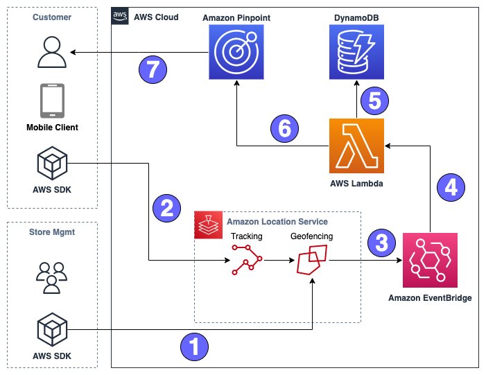
For our example use case, streaming data is coming through Amazon Kinesis Data Streams, and reference data is managed in MySQL. The reference data is continuously replicated from MySQL to DynamoDB through AWS DMS. The requirement here is to enrich the real-time stream data by joining with the reference data in near-real time, and to make it queryable from a query engine such as Amazon Athena while keeping consistency. In this use case, reference data in MySQL can be updated when the requirement is changed, and then queries need to return results by reflecting updates in the reference data.

This solution addresses the issue of users wanting to join streams with changing reference datasets when the size of the reference dataset is small. The reference data is maintained in DynamoDB tables, and the streaming job loads the full table into memory for each micro-batch, joining a high-throughput stream to a small reference dataset.

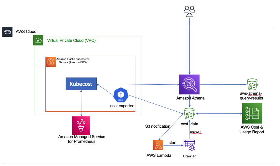
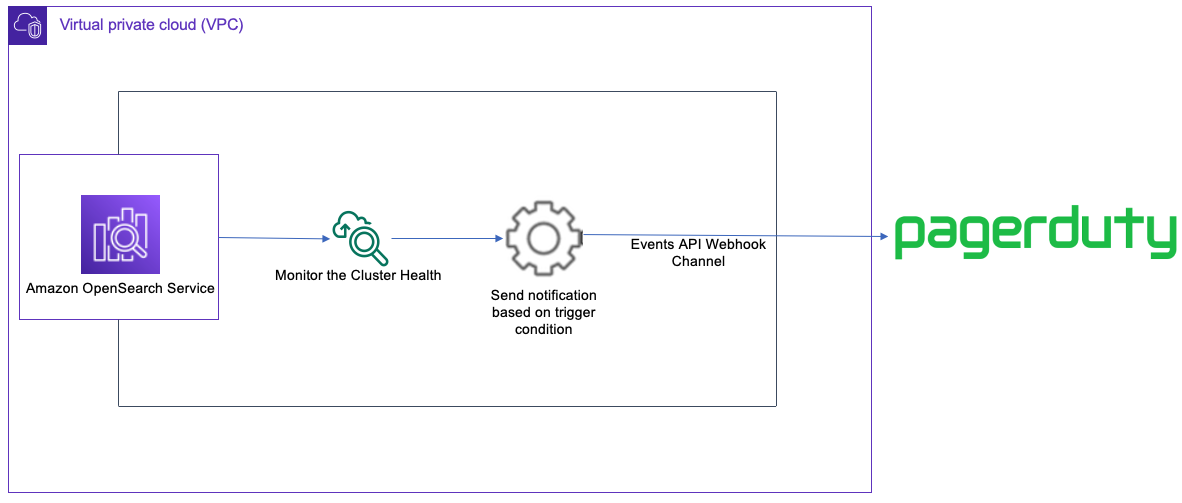
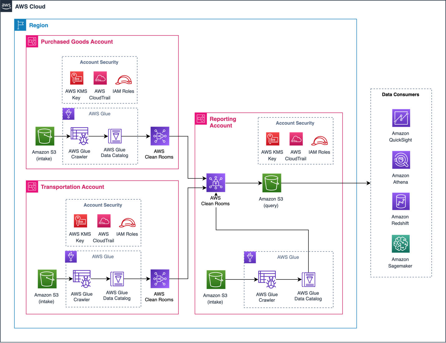
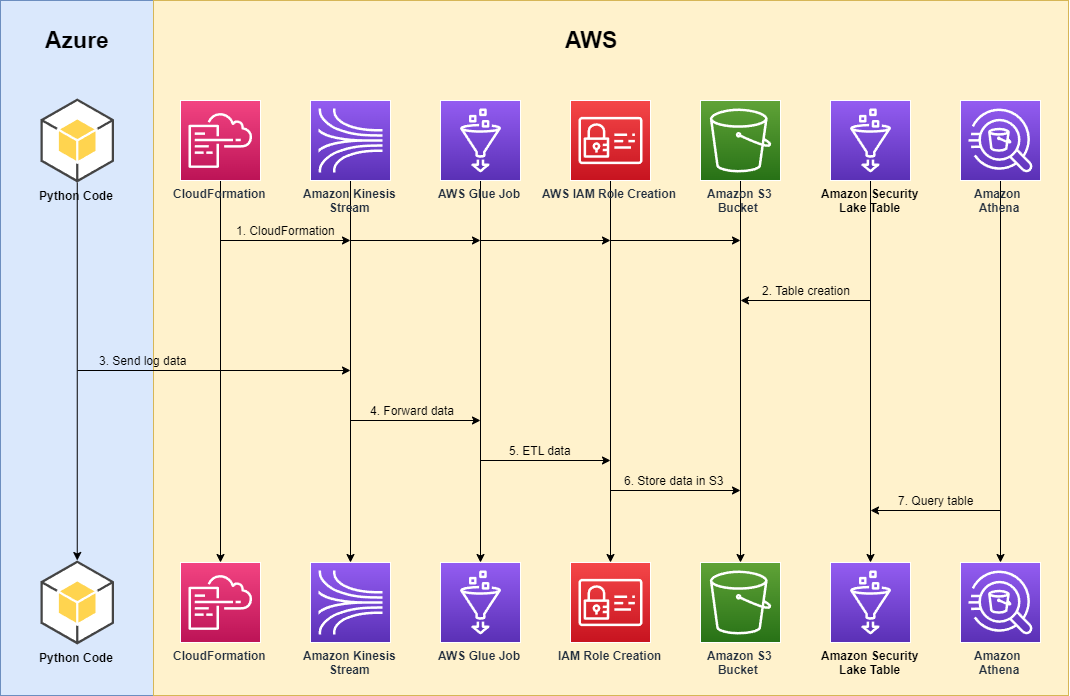
The following diagram illustrates the solution architecture.

Prerequisites

For this walkthrough, you should have the following prerequisites:

An AWS account.
A host with the installed MySQL utility, such as an Amazon Elastic Compute Cloud (Amazon EC2) instance, AWS Cloud9, your laptop, and so on. The host is used to access an Amazon Aurora MySQL-Compatible Edition cluster that you create and to run a Python script that sends sample records to the Kinesis data stream.

Create IAM roles and S3 bucket

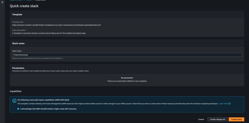
In this section, you create an Amazon Simple Storage Service (Amazon S3) bucket and two AWS Identity and Access Management (IAM) roles: one for the AWS Glue job, and one for AWS DMS. We do this using an AWS CloudFormation template. Complete the following steps:

Sign in to the AWS CloudFormation console.
Choose Launch Stack::
Choose Next.
For Stack name, enter a name for your stack.
For DynamoDBTableName, enter tgt_country_lookup_table. This is the name of your new DynamoDB table.
For S3BucketNamePrefix, enter the prefix of your new S3 bucket.
Select I acknowledge that AWS CloudFormation might create IAM resources with custom names.
Choose Create stack.

Stack creation can take about 1 minute.

Create a Kinesis data stream

In this section, you create a Kinesis data stream:

On the Kinesis console, choose Data streams in the navigation pane.
Choose Create data stream.
For Data stream name, enter your stream name.
Leave the remaining settings as default and choose Create data stream.

A Kinesis data stream is created with on-demand mode.

Create and configure an Aurora MySQL cluster

In this section, you create and configure an Aurora MySQL cluster as the source database. First, configure your source Aurora MySQL database cluster to enable CDC through AWS DMS to DynamoDB.

Create a parameter group

Complete the following steps to create a new parameter group:

On the Amazon RDS console, choose Parameter groups in the navigation pane.
Choose Create parameter group.
For Parameter group family, select aurora-mysql5.7.
For Type, choose DB Cluster Parameter Group.
For Group name, enter my-mysql-dynamodb-cdc.
For Description, enter Parameter group for demo Aurora MySQL database.
Choose Create.
Select my-mysql-dynamodb-cdc, and choose Edit under Parameter group actions.
Edit the parameter group as follows:

Name	Value
binlog_row_image	full
binlog_format	ROW
binlog_checksum	NONE
log_slave_updates	1

Choose Save changes.

Create the Aurora MySQL cluster

Complete following steps to create the Aurora MySQL cluster:

On the Amazon RDS console, choose Databases in the navigation pane.
Choose Create database.
For Choose a database creation method, choose Standard create.
Under Engine options, for Engine type, choose Aurora (MySQL Compatible).
For Engine version, choose Aurora (MySQL 5.7) 2.11.2.
For Templates, choose Production.
Under Settings, for DB cluster identifier, enter a name for your database.
For Master username, enter your primary user name.
For Master password and Confirm master password, enter your primary password.
Under Instance configuration, for DB instance class, choose Burstable classes (includes t classes) and choose db.t3.small.
Under Availability & durability, for Multi-AZ deployment, choose Don’t create an Aurora Replica.
Under Connectivity, for Compute resource, choose Don’t connect to an EC2 compute resource.
For Network type, choose IPv4.
For Virtual private cloud (VPC), choose your VPC.
For DB subnet group, choose your public subnet.
For Public access, choose Yes.
For VPC security group (firewall), choose the security group for your public subnet.
Under Database authentication, for Database authentication options, choose Password authentication.
Under Additional configuration, for DB cluster parameter group, choose the cluster parameter group you created earlier.
Choose Create database.

Grant permissions to the source database

The next step is to grant the required permission on the source Aurora MySQL database. Now you can connect to the DB cluster using the MySQL utility. You can run queries to complete the following tasks:

Create a demo database and table and run queries on the data
Grant permission for a user used by the AWS DMS endpoint

Complete the following steps:

Log in to the EC2 instance that you’re using to connect to your DB cluster.
Enter the following command at the command prompt to connect to the primary DB instance of your DB cluster:

$ mysql -h mycluster.cluster-123456789012.us-east-1.rds.amazonaws.com -P 3306 -u admin -p

Run the following SQL command to create a database:

> CREATE DATABASE mydev;

Run the following SQL command to create a table:

> use mydev; 
> CREATE TABLE country_lookup_table
(
code varchar(5),
countryname varchar(40) not null,
combinedname varchar(40) not null
);

Run the following SQL command to populate the table with data:

> INSERT INTO country_lookup_table(code, countryname, combinedname) VALUES ('IN', 'India', 'IN-India'), ('US', 'USA', 'US-USA'), ('CA', 'Canada', 'CA-Canada'), ('CN', 'China', 'CN-China');

Run the following SQL command to create a user for the AWS DMS endpoint and grant permissions for CDC tasks (replace the placeholder with your preferred password):

> CREATE USER repl IDENTIFIED BY '<your-password>';
> GRANT REPLICATION CLIENT, REPLICATION SLAVE ON *.* TO 'repl'@'%';
> GRANT SELECT ON mydev.country_lookup_table TO 'repl'@'%';

Create and configure AWS DMS resources to load data into the DynamoDB reference table

In this section, you create and configure AWS DMS to replicate data into the DynamoDB reference table.

Create an AWS DMS replication instance

First, create an AWS DMS replication instance by completing the following steps:

On the AWS DMS console, choose Replication instances in the navigation pane.
Choose Create replication instance.
Under Settings, for Name, enter a name for your instance.
Under Instance configuration, for High Availability, choose Dev or test workload (Single-AZ).
Under Connectivity and security, for VPC security groups, choose default.
Choose Create replication instance.

Create Amazon VPC endpoints

Optionally, you can create Amazon VPC endpoints for DynamoDB when you need to connect to your DynamoDB table from the AWS DMS instance in a private network. Also make sure that you enable Publicly accessible when you need to connect to a database outside of your VPC.

Create an AWS DMS source endpoint

Create an AWS DMS source endpoint by completing the following steps:

On the AWS DMS console, choose Endpoints in the navigation pane.
Choose Create endpoint.
For Endpoint type, choose Source endpoint.
Under Endpoint configuration, for Endpoint identifier, enter a name for your endpoint.
For Source engine, choose Amazon Aurora MySQL.
For Access to endpoint database, choose Provide access information manually.
For Server Name, enter the endpoint name of your Aurora writer instance (for example, mycluster.cluster-123456789012.us-east-1.rds.amazonaws.com).
For Port, enter 3306.
For User name, enter a user name for your AWS DMS task.
For Password, enter a password.
Choose Create endpoint.

Crate an AWS DMS target endpoint

Create an AWS DMS target endpoint by completing the following steps:

On the AWS DMS console, choose Endpoints in the navigation pane.
Choose Create endpoint.
For Endpoint type, choose Target endpoint.
Under Endpoint configuration, for Endpoint identifier, enter a name for your endpoint.
For Target engine, choose Amazon DynamoDB.
For Service access role ARN, enter the IAM role for your AWS DMS task.
Choose Create endpoint.

Create AWS DMS migration tasks

Create AWS DMS database migration tasks by completing the following steps:

On the AWS DMS console, choose Database migration tasks in the navigation pane.
Choose Create task.
Under Task configuration, for Task identifier, enter a name for your task.
For Replication instance, choose your replication instance.
For Source database endpoint, choose your source endpoint.
For Target database endpoint, choose your target endpoint.
For Migration type, choose Migrate existing data and replicate ongoing changes.
Under Task settings, for Target table preparation mode, choose Do nothing.
For Stop task after full load completes, choose Don’t stop.
For LOB column settings, choose Limited LOB mode.
For Task logs, enable Turn on CloudWatch logs and Turn on batch-optimized apply.
Under Table mappings, choose JSON Editor and enter the following rules.

Here you can add values to the column. With the following rules, the AWS DMS CDC task will first create a new DynamoDB table with the specified name in target-table-name. Then it will replicate all the records, mapping the columns in the DB table to the attributes in the DynamoDB table.

{
    "rules": [
        {
            "rule-type": "selection",
            "rule-id": "1",
            "rule-name": "1",
            "object-locator": {
                "schema-name": "mydev",
                "table-name": "country_lookup_table"
            },
            "rule-action": "include"
        },
        {
            "rule-type": "object-mapping",
            "rule-id": "2",
            "rule-name": "2",
            "rule-action": "map-record-to-record",
            "object-locator": {
                "schema-name": "mydev",
                "table-name": "country_lookup_table"
            },
            "target-table-name": "tgt_country_lookup_table",
            "mapping-parameters": {
                "partition-key-name": "code",
                "sort-key-name": "countryname",
                "exclude-columns": [
                    "code",
                    "countryname"
                ],
                "attribute-mappings": [
                    {
                        "target-attribute-name": "code",
                        "attribute-type": "scalar",
                        "attribute-sub-type": "string",
                        "value": "${code}"
                    },
                    {
                        "target-attribute-name": "countryname",
                        "attribute-type": "scalar",
                        "attribute-sub-type": "string",
                        "value": "${countryname}"
                    }
                ],
                "apply-during-cdc": true
            }
        }
    ]
}

Choose Create task.

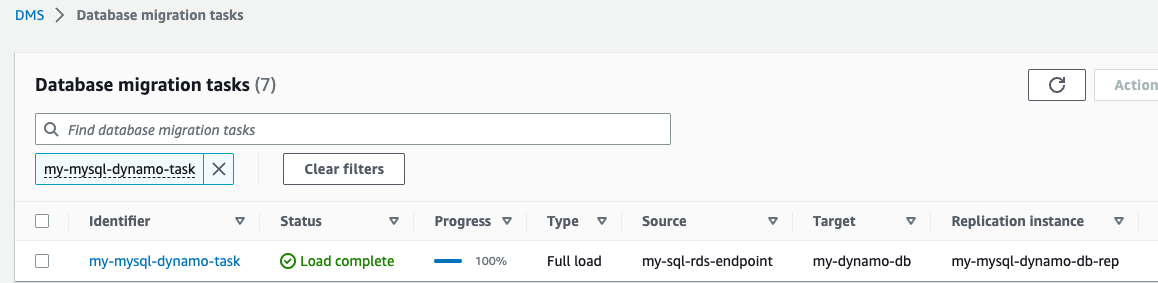
Now the AWS DMS replication task has been started.

Wait for the Status to show as Load complete.

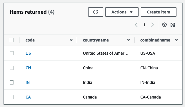
On the DynamoDB console, choose Tables in the navigation pane.
Select the DynamoDB reference table, and choose Explore table items to review the replicated records.

Create an AWS Glue Data Catalog table and an AWS Glue streaming ETL job

In this section, you create an AWS Glue Data Catalog table and an AWS Glue streaming extract, transform, and load (ETL) job.

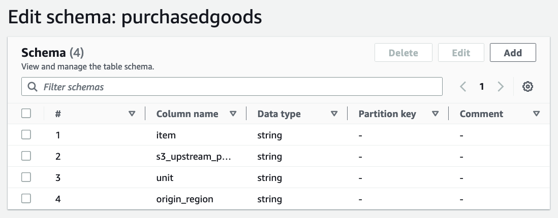
Create a Data Catalog table

Create an AWS Glue Data Catalog table for the source Kinesis data stream with the following steps:

On the AWS Glue console, choose Databases under Data Catalog in the navigation pane.
Choose Add database.
For Name, enter my_kinesis_db.
Choose Create database.
Choose Tables under Databases, then choose Add table.
For Name, enter my_stream_src_table.
For Database, choose my_kinesis_db.
For Select the type of source, choose Kinesis.
For Kinesis data stream is located in, choose my account.
For Kinesis stream name, enter a name for your data stream.
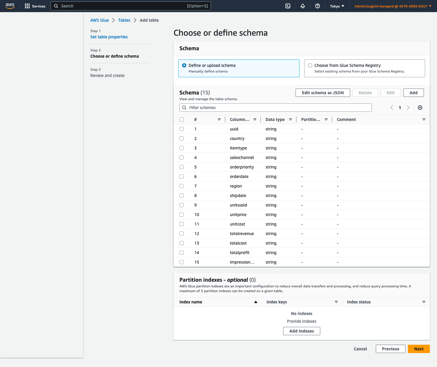
For Classification, select JSON.
Choose Next.
Choose Edit schema as JSON, enter the following JSON, then choose Save.

[
  {
    "Name": "uuid",
    "Type": "string",
    "Comment": ""
  },
  {
    "Name": "country",
    "Type": "string",
    "Comment": ""
  },
  {
    "Name": "itemtype",
    "Type": "string",
    "Comment": ""
  },
  {
    "Name": "saleschannel",
    "Type": "string",
    "Comment": ""
  },
  {
    "Name": "orderpriority",
    "Type": "string",
    "Comment": ""
  },
  {
    "Name": "orderdate",
    "Type": "string",
    "Comment": ""
  },
  {
    "Name": "region",
    "Type": "string",
    "Comment": ""
  },
  {
    "Name": "shipdate",
    "Type": "string",
    "Comment": ""
  },
  {
    "Name": "unitssold",
    "Type": "string",
    "Comment": ""
  },
  {
    "Name": "unitprice",
    "Type": "string",
    "Comment": ""
  },
  {
    "Name": "unitcost",
    "Type": "string",
    "Comment": ""
  },
  {
    "Name": "totalrevenue",
    "Type": "string",
    "Comment": ""
  },
  {
    "Name": "totalcost",
    "Type": "string",
    "Comment": ""
  },
  {
    "Name": "totalprofit",
    "Type": "string",
    "Comment": ""
  },
  {
    "Name": "impressiontime",
    "Type": "string",
    "Comment": ""
  }
]

1. Choose Next, then choose Create.

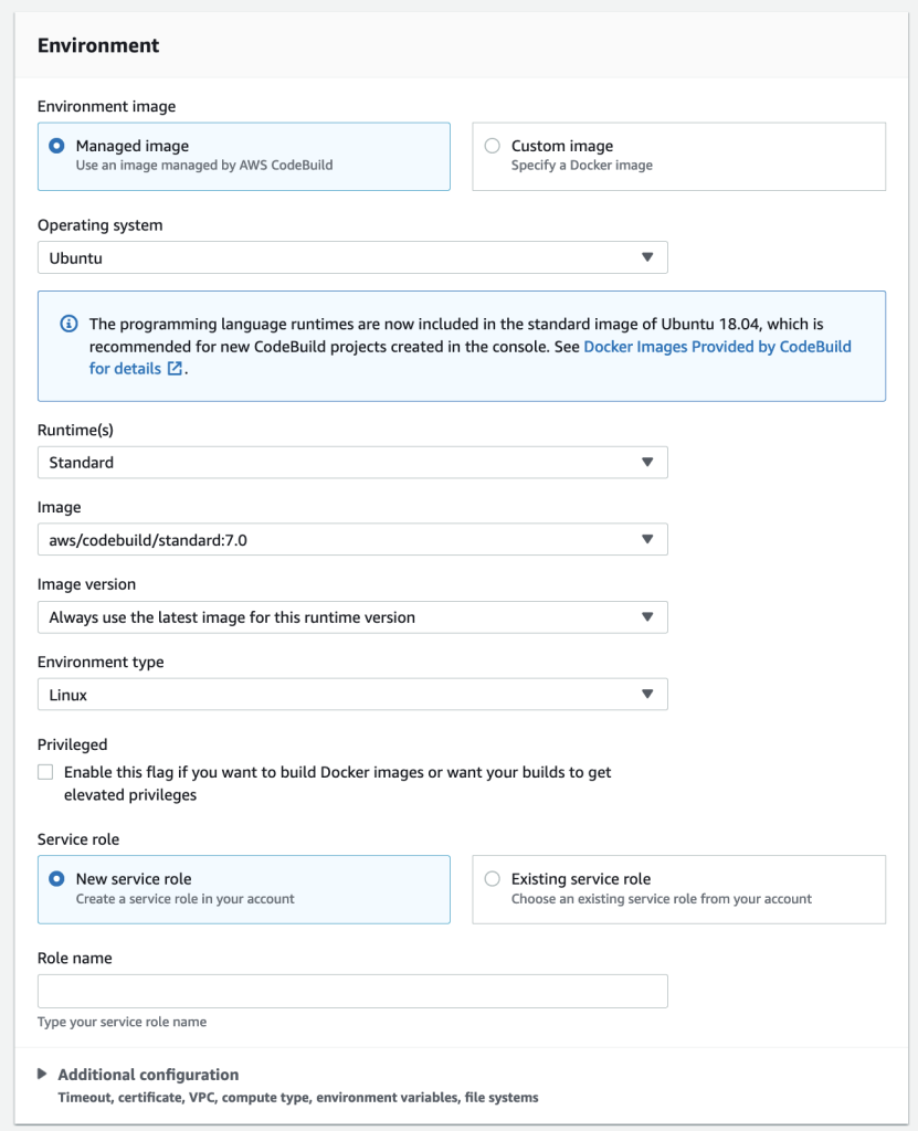
Create an AWS Glue streaming ETL job

Next, you create an AWS Glue streaming job. AWS Glue 3.0 and later supports Apache Hudi natively, so we use this native integration to ingest into a Hudi table. Complete the following steps to create the AWS Glue streaming job:

On the AWS Glue Studio console, choose Spark script editor and choose Create.
Under Job details tab, for Name, enter a name for your job.
For IAM Role, choose the IAM role for your AWS Glue job.
For Type, select Spark Streaming.
For Glue version, choose Glue 4.0 – Supports spark 3.3, Scala 2, Python 3.
For Requested number of workers, enter 3.
Under Advanced properties, for Job parameters, choose Add new parameter.
For Key, enter --conf.
For Value, enter spark.serializer=org.apache.spark.serializer.KryoSerializer --conf spark.sql.hive.convertMetastoreParquet=false.
Choose Add new parameter.
For Key, enter --datalake-formats.
For Value, enter hudi.
For Script path, enter s3://<S3BucketName>/scripts/.
For Temporary path, enter s3://<S3BucketName>/temporary/.
Optionally, for Spark UI logs path, enter s3://<S3BucketName>/sparkHistoryLogs/.

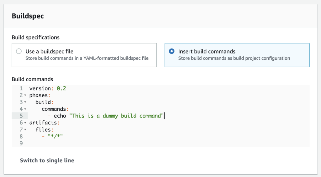
On the Script tab, enter the following script into the AWS Glue Studio editor and choose Create.

The near-real-time streaming job enriches data by joining a Kinesis data stream with a DynamoDB table that contains frequently updated reference data. The enriched dataset is loaded into the target Hudi table in the data lake. Replace <S3BucketName> with your bucket that you created via AWS CloudFormation:

import sys, json
import boto3
from pyspark.sql import DataFrame, Row
from pyspark.context import SparkContext
from pyspark.sql.types import *
from pyspark.sql.functions import *
from awsglue.transforms import *
from awsglue.utils import getResolvedOptions
from awsglue.context import GlueContext
from awsglue.job import Job

args = getResolvedOptions(sys.argv,["JOB_NAME"])

# Initialize spark session and Glue context
sc = SparkContext() 
glueContext = GlueContext(sc)
spark = glueContext.spark_session
job = Job(glueContext)
job.init(args["JOB_NAME"], args)

# job paramters
dydb_lookup_table = "tgt_country_lookup_table"
kin_src_database_name = "my_kinesis_db" 
kin_src_table_name = "my_stream_src_table" 
hudi_write_operation = "upsert" 
hudi_record_key = "uuid" 
hudi_precomb_key = "orderdate" 
checkpoint_path = "s3://<S3BucketName>/streamlab/checkpoint/" 
s3_output_folder = "s3://<S3BucketName>/output/"
hudi_table = "hudi_table"
hudi_database = "my_kinesis_db"

# hudi options 
additional_options={
    "hoodie.datasource.hive_sync.use_jdbc": "false",
    "hoodie.datasource.write.recordkey.field": hudi_record_key,
    "hoodie.datasource.hive_sync.database": hudi_database,
    "hoodie.table.name": hudi_table,
    "hoodie.consistency.check.enabled": "true",
    "hoodie.datasource.write.keygenerator.class": "org.apache.hudi.keygen.NonpartitionedKeyGenerator",
    "hoodie.datasource.hive_sync.partition_extractor_class": "org.apache.hudi.hive.NonPartitionedExtractor",
    "hoodie.datasource.write.hive_style_partitioning": "false",
    "hoodie.datasource.write.precombine.field": hudi_precomb_key,
    "hoodie.bulkinsert.shuffle.parallelism": "4",
    "hoodie.datasource.hive_sync.enable": "true",
    "hoodie.datasource.write.operation": hudi_write_operation,
    "hoodie.datasource.write.storage.type": "COPY_ON_WRITE",
}

# Scan and load the reference data table from DynamoDB into AWS Glue DynamicFrames using boto3 API.
def readDynamoDb():
    dynamodb = boto3.resource(“dynamodb”)
    table = dynamodb.Table(dydb_lookup_table)
    response = table.scan()
    items = response[“Items”]
    jsondata = sc.parallelize(items)
    lookupDf = glueContext.read.json(jsondata)
    return lookupDf


# Load the Amazon Kinesis data stream from Amazon Glue Data Catalog.
source_df = glueContext.create_data_frame.from_catalog(
    database=kin_src_database_name,
    table_name=kin_src_table_name,
    transformation_ctx=”source_df”,
    additional_options={“startingPosition”: “TRIM_HORIZON”},
)

# As part of batch processing, implement the transformation logic for joining streaming data frames with reference data frames.
def processBatch(data_frame, batchId):
    if data_frame.count() > 0:

        # Refresh the dymanodb table to pull latest snapshot for each microbatch
        country_lookup_df = readDynamoDb() 
                
        final_frame = data_frame.join(
            country_lookup_df, 
            data_frame["country"] == country_lookup_df["countryname"], 
            'left'
        ).drop(
            "countryname",
            "country",
            "unitprice", 
            "unitcost",
            "totalrevenue",
            "totalcost",
            "totalprofit"
        )

        # Script generated for node my-lab-hudi-connector
        final_frame.write.format("hudi") \
            .options(**additional_options) \
            .mode("append") \
            .save(s3_output_folder)
        
try:
    glueContext.forEachBatch(
        frame=source_df,
        batch_function=processBatch,
        options={"windowSize": "60 seconds", "checkpointLocation": checkpoint_path},
    )
except Exception as e:
    print(f"Error is @@@ ....{e}")

Choose Run to start the streaming job.

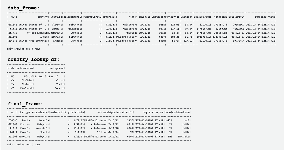
The following screenshot shows examples of the DataFrames data_frame, country_lookup_df, and final_frame.

The AWS Glue job successfully joined records coming from the Kinesis data stream and the reference table in DynamoDB, and then ingested the joined records into Amazon S3 in Hudi format.

Create and run a Python script to generate sample data and load it into the Kinesis data stream

In this section, you create and run a Python to generate sample data and load it into the source Kinesis data stream. Complete the following steps:

Log in to AWS Cloud9, your EC2 instance, or any other computing host that puts records in your data stream.
Create a Python file called generate-data-for-kds.py:

$ python3 generate-data-for-kds.py

Open the Python file and enter the following script:

import json
import random
import boto3
import time

STREAM_NAME = "<mystreamname>"

def get_data():
    return {
        "uuid": random.randrange(0, 1000001, 1),
        "country": random.choice( [ "United Arab Emirates", "China", "India", "United Kingdom", "United States of America", ] ),
        "itemtype": random.choice( [ "Snacks", "Cereals", "Cosmetics", "Fruits", "Clothes", "Babycare", "Household", ] ),
        "saleschannel": random.choice( [ "Snacks", "Cereals", "Cosmetics", "Fruits", "Clothes", "Babycare", "Household", ] ),
        "orderpriority": random.choice(["H", "L", "M", "C"]),
        "orderdate": random.choice( [ "1/4/10", "2/28/10", "2/15/11", "11/8/11", "2/1/12", "2/18/12", "3/1/12", "9/24/12",
                                      "10/13/12", "12/2/12", "12/29/12", "3/30/13", "7/29/13", "3/23/14", "6/14/14", 
                                      "7/15/14", "10/19/14", "5/7/15", "10/11/15", "11/22/15", "8/23/16", "1/15/17", 
                                      "1/27/17", "2/25/17", "3/10/17", "4/1/17", ] ),
        "region": random.choice( ["Asia" "Europe", "Americas", "Middle Eastern", "Africa"] ),
        "shipdate": random.choice( [ "1/4/10", "2/28/10", "2/15/11", "11/8/11", "2/1/12", "2/18/12", "3/1/12", "9/24/12", 
                                    "10/13/12", "12/2/12", "12/29/12", "3/30/13", "7/29/13", "3/23/14", "6/14/14", "7/15/14",
                                      "10/19/14", "5/7/15", "10/11/15", "11/22/15", "8/23/16", "1/15/17", "1/27/17", 
                                      "2/25/17", "3/10/17", "4/1/17", ] ),
        "unitssold": random.choice( [ "8217", "3465", "8877", "2882", "70", "7044", "6307", "2384", "1327", "2572", "8794", 
                                     "4131", "5793", "9091", "4314", "9085", "5270", "5459", "1982", "8245", "4860", "4656", 
                                     "8072", "65", "7864", "9778", ] ),
        "unitprice": random.choice( [ "97.44", "117.11", "364.69", "502.54", "263.33", "117.11", "35.84", "6.92", "35.84", 
                                     "6.92", "35.84", "56.67", "159.42", "502.54", "117.11", "56.67", "524.96", "502.54", 
                                     "56.67", "56.67", "159.42", "56.67", "35.84", "159.42", "502.54", "31.79", ] ),
        "unitcost": random.choice( [ "97.44", "117.11", "364.69", "502.54", "263.33", "117.11", "35.84", "6.92", "35.84", 
                                    "6.92", "35.84", "56.67", "159.42", "502.54", "117.11", "56.67", "524.96", "502.54", 
                                    "56.67", "56.67", "159.42", "56.67", "35.84", "159.42", "502.54", "31.79", ] ),
        "totalrevenue": random.choice( [ "1253749.86", "712750.5", "3745117.53", "1925954.14", "30604", "1448950.8", 
                                        "689228.96", "22242.72", "145014.56", "23996.76", "961008.32", "337626.63", 
                                        "1478837.04", "6075242.57", "887389.8", "742517.05", "3431876.7", "3648085.93", 
                                        "161988.86", "673863.85", "1240660.8", "380534.88", "882108.16", "16593.2", 
                                        "5255275.28", "463966.1", ] ),
        "totalcost": random.choice( [ "800664.48", "405786.15", "3237353.13", "1448320.28", "18433.1", "824922.84", 
                                     "226042.88", "16497.28", "47559.68", "17798.24", "315176.96", "234103.77", "923520.06",
                                       "4568591.14", "505212.54", "514846.95", "2766539.2", "2743365.86", 
                                       "112319.94", "467244.15", "774781.2", "263855.52", "289300.48", "10362.3", 
                                       "3951974.56", "310842.62", ] ),
        "totalprofit": random.choice( [ "453085.38", "306964.35", "507764.4", "477633.86", "12170.9", "624027.96", 
                                       "463186.08", "5745.44", "97454.88", "6198.52", "645831.36", "103522.86", "555316.98", 
                                       "1506651.43", "382177.26", "227670.1", "665337.5", "904720.07", "49668.92", "206619.7",
                                         "465879.6", "116679.36", "592807.68", "6230.9", "1303300.72", "153123.48", ] ),
        "impressiontime": random.choice( [ "2022-10-24T02:27:41Z", "2022-10-24T02:27:41Z", "2022-11-24T02:27:41Z", 
                                          "2022-12-24T02:27:41Z", "2022-13-24T02:27:41Z", "2022-14-24T02:27:41Z", 
                                          "2022-15-24T02:27:41Z", ] ),
    }

def generate(stream_name, kinesis_client):
    while True:
        data = get_data()
        print(data)
        kinesis_client.put_record(
            StreamName=stream_name, Data=json.dumps(data), PartitionKey="partitionkey"
        )
        time.sleep(2)

if __name__ == "__main__":
    generate(STREAM_NAME, boto3.client("kinesis"))

This script puts a Kinesis data stream record every 2 seconds.

Simulate updating the reference table in the Aurora MySQL cluster

Now all the resources and configurations are ready. For this example, we want to add a 3-digit country code to the reference table. Let’s update records in the Aurora MySQL table to simulate changes. Complete the following steps:

Make sure that the AWS Glue streaming job is already running.
Connect to the primary DB instance again, as described earlier.
Enter your SQL commands to update records:

> UPDATE country_lookup_table SET combinedname='US-USA-US' WHERE code='US';
> UPDATE country_lookup_table SET combinedname='CA-CAN-Canada' WHERE code='CA';
> UPDATE country_lookup_table SET combinedname='CN-CHN-China' WHERE code='CN';
> UPDATE country_lookup_table SET combinedname='IN-IND-India' WHERE code='IN';

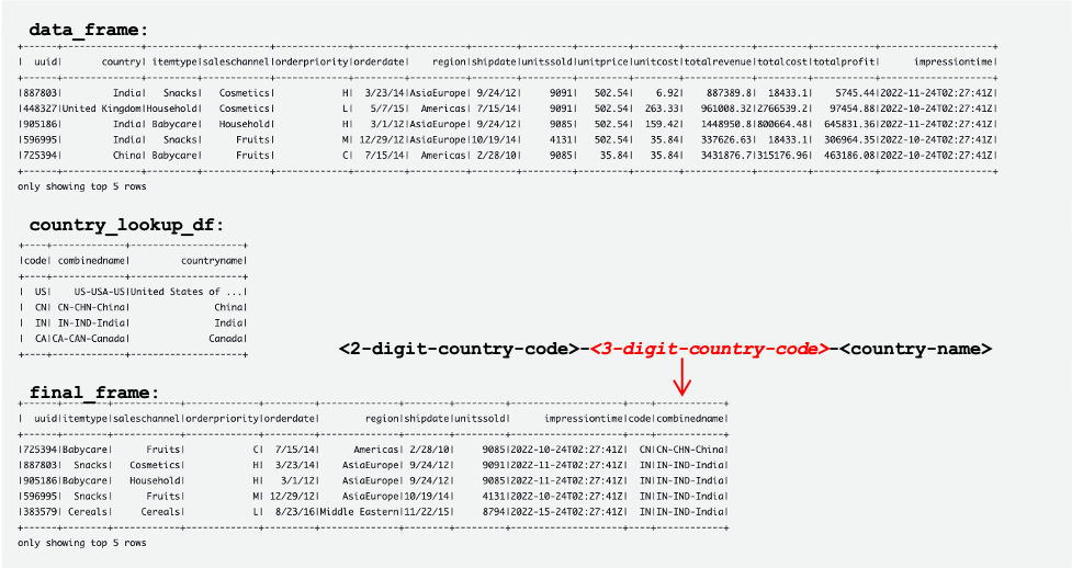
Now the reference table in the Aurora MySQL source database has been updated. Then the changes are automatically replicated to the reference table in DynamoDB.

The following tables show records in data_frame, country_lookup_df, and final_frame. In country_lookup_df and final_frame, the combinedname column has values formatted as <2-digit-country-code>-<3-digit-country-code>-<country-name>, which shows that the changed records in the referenced table are reflected in the table without restarting the AWS Glue streaming job. It means that the AWS Glue job successfully joins the incoming records from the Kinesis data stream with the reference table even when the reference table is changing.

Query the Hudi table using Athena

Let’s query the Hudi table using Athena to see the records in the destination table. Complete the following steps:

Make sure that the script and the AWS Glue Streaming job is still working:
1. The Python script (generate-data-for-kds.py) is still running.
2. The generated data is being sent to the data stream.
3. The AWS Glue streaming job is still running.
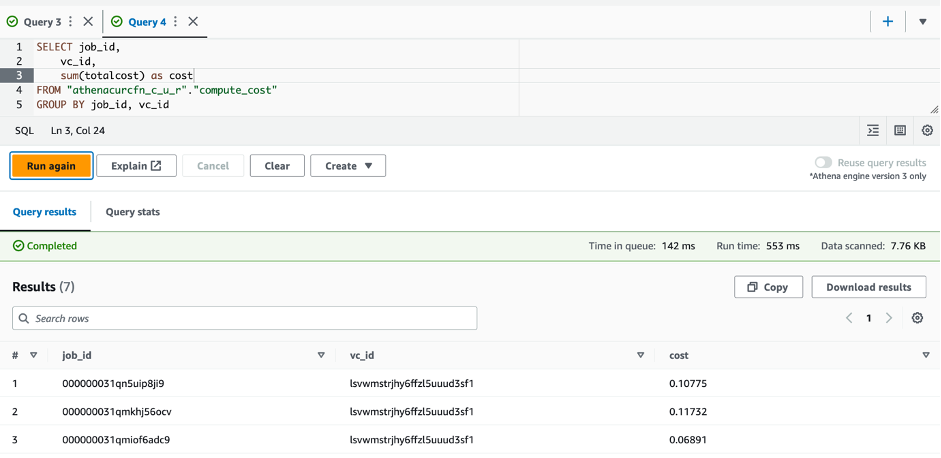
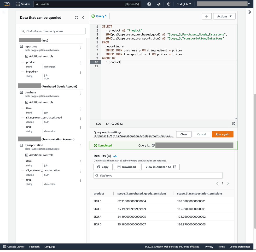
On the Athena console, run the following SQL in the query editor:

select shipdate, unitssold, impressiontime, code,combinedname from <database>.<table>
where combinedname is not null
limit 10;

The following query result shows the records that are processed before the referenced table was changed. Records in the combinedname column are similar to <2-digit-country-code>-<country-name>.

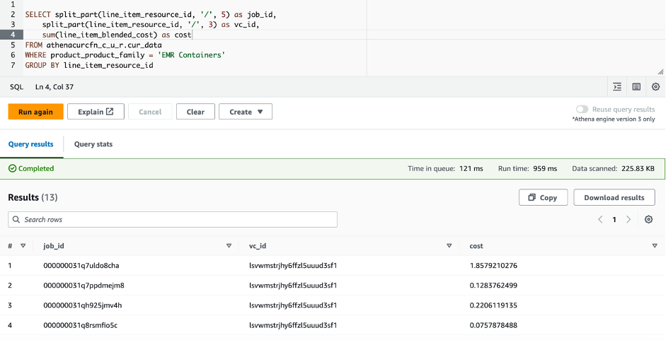
The following query result shows the records that are processed after the referenced table was changed. Records in the combinedname column are similar to <2-digit-country-code>-<3-digit-country-code>-<country-name>.

Now you understand that the changed reference data is successfully reflected in the target Hudi table joining records from the Kinesis data stream and the reference data in DynamoDB.

Clean up

As the final step, clean up the resources:

Delete the Kinesis data stream.
Delete the AWS DMS migration task, endpoint, and replication instance.
Stop and delete the AWS Glue streaming job.
Delete the AWS Cloud9 environment.
Delete the CloudFormation template.

Conclusion

Building and maintaining a transactional data lake that involves real-time data ingestion and processing has multiple variable components and decisions to be made, such as what ingestion service to use, how to store your reference data, and what transactional data lake framework to use. In this post, we provided the implementation details of such a pipeline, using AWS native components as the building blocks and Apache Hudi as the open-source framework for a transactional data lake.

We believe that this solution can be a starting point for organizations looking to implement a new data lake with such requirements. Additionally, the different components are fully pluggable and can be mixed and matched to existing data lakes to target new requirements or migrate existing ones, addressing their pain points.

About the authors

Manish Kola is a Data Lab Solutions Architect at AWS, where he works closely with customers across various industries to architect cloud-native solutions for their data analytics and AI needs. He partners with customers on their AWS journey to solve their business problems and build scalable prototypes. Before joining AWS, Manish’s experience includes helping customers implement data warehouse, BI, data integration, and data lake projects.

Santosh Kotagiri is a Solutions Architect at AWS with experience in data analytics and cloud solutions leading to tangible business results. His expertise lies in designing and implementing scalable data analytics solutions for clients across industries, with a focus on cloud-native and open-source services. He is passionate about leveraging technology to drive business growth and solve complex problems.

Chiho Sugimoto is a Cloud Support Engineer on the AWS Big Data Support team. She is passionate about helping customers build data lakes using ETL workloads. She loves planetary science and enjoys studying the asteroid Ryugu on weekends.

Noritaka Sekiyama is a Principal Big Data Architect on the AWS Glue team. He is responsible for building software artifacts to help customers. In his spare time, he enjoys cycling with his new road bike.

Introducing the Enhanced Document API for DynamoDB in the AWS SDK for Java 2.x

2023-05-26 John Viegas

Post Syndicated from John Viegas original https://aws.amazon.com/blogs/devops/introducing-the-enhanced-document-api-for-dynamodb-in-the-aws-sdk-for-java-2-x/

We are excited to announce that the AWS SDK for Java 2.x now offers the Enhanced Document API for DynamoDB, providing an enhanced way of working with Amazon DynamoDb items.
This post covers using the Enhanced Document API for DynamoDB with the DynamoDB Enhanced Client. By using the Enhanced Document API, you can create an EnhancedDocument instance to represent an item with no fixed schema, and then use the DynamoDB Enhanced Client to read and write to DynamoDB.
Furthermore, unlike the Document APIs of aws-sdk-java 1.x, which provided arguments and return types that were not type-safe, the EnhancedDocument provides strongly-typed APIs for working with documents. This interface simplifies the development process and ensures that the data is correctly typed.

Prerequisites:

Before getting started, ensure you are using an up-to-date version of the AWS Java SDK dependency with all the latest released bug-fixes and features. For Enhanced Document API support, you must use version 2.20.33 or later. See our “Set up an Apache Maven project” guide for details on how to manage the AWS Java SDK dependency in your project.

Add dependency for dynamodb-enhanced in pom.xml.

<dependency>
<groupId>software.amazon.awssdk</groupId>
<artifactId>dynamodb-enhanced</artifactId>
<version>2.20.33</version>
</dependency>

Quick walk-through for using Enhanced Document API to interact with DDB

Step 1 : Create a DynamoDB Enhanced Client

Create an instance of the DynamoDbEnhancedClient class, which provides a high-level interface for Amazon DynamoDB that simplifies working with DynamoDB tables.

DynamoDbEnhancedClient enhancedClient = DynamoDbEnhancedClient.builder()
                                               .dynamoDbClient(DynamoDbClient.create())
                                               .build();

Step 2 : Create a DynamoDbTable resource object with Document table schema

To execute commands against a DynamoDB table using the Enhanced Document API, you must associate the table with your Document table schema to create a DynamoDbTable resource object. The Document table schema builder requires the primary index key and attribute converter providers. Use AttributeConverterProvider.defaultProvider() to convert document attributes of default types. An optional secondary index key can be added to the builder.


DynamoDbTable<EnhancedDocument> documentTable = enhancedClient.table("my_table",
                                              TableSchema.documentSchemaBuilder()
                                                         .addIndexPartitionKey(TableMetadata.primaryIndexName(),"hashKey", AttributeValueType.S)
                                                         .addIndexSortKey(TableMetadata.primaryIndexName(), "sortKey", AttributeValueType.N)
                                                         .attributeConverterProviders(AttributeConverterProvider.defaultProvider())
                                                         .build());
                                                         
// call documentTable.createTable() if "my_table" does not exist in DynamoDB

Step 3 : Write a DynamoDB item using an EnhancedDocument

The EnhancedDocument class has static factory methods along with a builder method to add attributes to a document. The following snippet demonstrates the type safety provided by EnhancedDocument when you construct a document item.

EnhancedDocument simpleDoc = EnhancedDocument.builder()
 .attributeConverterProviders(defaultProvider())
 .putString("hashKey", "sampleHash")
 .putNull("nullKey")
 .putNumber("sortKey", 1.0)
 .putBytes("byte", SdkBytes.fromUtf8String("a"))
 .putBoolean("booleanKey", true)
 .build();
 
documentTable.putItem(simpleDoc);

Step 4 : Read a Dynamo DB item as an EnhancedDocument

Attributes of the Documents retrieved from a DynamoDB table can be accessed with getter methods

EnhancedDocument docGetItem = documentTable.getItem(r -> r.key(k -> k.partitionValue("samppleHash").sortValue(1)));

docGetItem.getString("hashKey");
docGetItem.isNull("nullKey")
docGetItem.getNumber("sortKey").floatValue();
docGetItem.getBytes("byte");
docGetItem.getBoolean("booleanKey");

AttributeConverterProviders for accessing document attributes as custom objects

You can provide a custom AttributeConverterProvider instance to an EnhancedDocument to convert document attributes to a specific object type.
These providers can be set on either DocumentTableSchema or EnhancedDocument to read or write attributes as custom objects.

TableSchema.documentSchemaBuilder()
           .attributeConverterProviders(CustomClassConverterProvider.create(), defaultProvider())
           .build();
    
// Insert a custom class instance into an EnhancedDocument as attribute 'customMapOfAttribute'.
EnhancedDocument customAttributeDocument =
EnhancedDocument.builder().put("customMapOfAttribute", customClassInstance, CustomClass.class).build();

// Retrieve attribute 'customMapOfAttribute' as CustomClass object.
CustomClass customClassObject = customAttributeDocument.get("customMapOfAttribute", CustomClass.class);

Convert Documents to JSON and vice-versa

The Enhanced Document API allows you to convert a JSON string to an EnhancedDocument and vice-versa.

// Enhanced document created from JSON string using defaultConverterProviders.
EnhancedDocument documentFromJson = EnhancedDocument.fromJson("{\"key\": \"Value\"}")
                                              
// Converting an EnhancedDocument to JSON string "{\"key\": \"Value\"}"                                                 
String jsonFromDocument = documentFromJson.toJson();

Define a Custom Attribute Converter Provider

Custom attribute converter providers are implementations of AttributeConverterProvider that provide converters for custom classes.
Below is an example for a CustomClassForDocumentAPI which has as a single field stringAttribute of type String and its corresponding AttributeConverterProvider implementation.

public class CustomClassForDocumentAPI {
    private final String stringAttribute;

    public CustomClassForDocumentAPI(Builder builder) {
        this.stringAttribute = builder.stringAttribute;
    }
    public static Builder builder() {
        return new Builder();
    }
    public String stringAttribute() {
        return stringAttribute;
    }
    public static final class Builder {
        private String stringAttribute;
        private Builder() {
        }
        public Builder stringAttribute(String stringAttribute) {
            this.stringAttribute = string;
            return this;
        }
        public CustomClassForDocumentAPI build() {
            return new CustomClassForDocumentAPI(this);
        }
    }
}

import java.util.Map;
import software.amazon.awssdk.enhanced.dynamodb.AttributeConverter;
import software.amazon.awssdk.enhanced.dynamodb.AttributeConverterProvider;
import software.amazon.awssdk.enhanced.dynamodb.EnhancedType;
import software.amazon.awssdk.utils.ImmutableMap;

public class CustomAttributeForDocumentConverterProvider implements AttributeConverterProvider {
    private final Map<EnhancedType<?>, AttributeConverter<?>> converterCache = ImmutableMap.of(
        EnhancedType.of(CustomClassForDocumentAPI.class), new CustomClassForDocumentAttributeConverter());
        // Different types of converters can be added to this map.

    public static CustomAttributeForDocumentConverterProvider create() {
        return new CustomAttributeForDocumentConverterProvider();
    }

    @Override
    public <T> AttributeConverter<T> converterFor(EnhancedType<T> enhancedType) {
        return (AttributeConverter<T>) converterCache.get(enhancedType);
    }
}

A custom attribute converter is an implementation of AttributeConverter that converts a custom classes to and from a map of attribute values, as shown below.

import java.util.LinkedHashMap;
import java.util.Map;
import software.amazon.awssdk.enhanced.dynamodb.AttributeConverter;
import software.amazon.awssdk.enhanced.dynamodb.AttributeValueType;
import software.amazon.awssdk.enhanced.dynamodb.EnhancedType;
import software.amazon.awssdk.enhanced.dynamodb.internal.converter.attribute.EnhancedAttributeValue;
import software.amazon.awssdk.enhanced.dynamodb.internal.converter.attribute.StringAttributeConverter;
import software.amazon.awssdk.services.dynamodb.model.AttributeValue;

public class CustomClassForDocumentAttributeConverter implements AttributeConverter<CustomClassForDocumentAPI> {
    public static CustomClassForDocumentAttributeConverter create() {
        return new CustomClassForDocumentAttributeConverter();
    }
    @Override
    public AttributeValue transformFrom(CustomClassForDocumentAPI input) {
        Map<String, AttributeValue> attributeValueMap = new LinkedHashMap<>();
        if(input.string() != null){
            attributeValueMap.put("stringAttribute", AttributeValue.fromS(input.string()));
        }
        return EnhancedAttributeValue.fromMap(attributeValueMap).toAttributeValue();
    }

    @Override
    public CustomClassForDocumentAPI transformTo(AttributeValue input) {
        Map<String, AttributeValue> customAttr = input.m();
        CustomClassForDocumentAPI.Builder builder = CustomClassForDocumentAPI.builder();
        if (customAttr.get("stringAttribute") != null) {
            builder.stringAttribute(StringAttributeConverter.create().transformTo(customAttr.get("stringAttribute")));
        }
        return builder.build();
    }
    @Override
    public EnhancedType<CustomClassForDocumentAPI> type() {
        return EnhancedType.of(CustomClassForDocumentAPI.class);
    }
    @Override
    public AttributeValueType attributeValueType() {
        return AttributeValueType.M;
    }
}

Attribute Converter Provider for EnhancedDocument Builder

When working outside of a DynamoDB table context, make sure to set the attribute converter providers explicitly on the EnhancedDocument builder. When used within a DynamoDB table context, the table schema’s converter provider will be used automatically for the EnhancedDocument.
The code snippet below shows how to set an AttributeConverterProvider using the EnhancedDocument builder method.

// Enhanced document created from JSON string using custom AttributeConverterProvider.
EnhancedDocument documentFromJson = EnhancedDocument.builder()
                                                    .attributeConverterProviders(CustomClassConverterProvider.create())
                                                    .json("{\"key\": \"Values\"}")
                                                    .build();
                                                    
CustomClassForDocumentAPI customClass = documentFromJson.get("key", CustomClassForDocumentAPI.class)

Conclusion

In this blog post we showed you how to set up and begin using the Enhanced Document API with the DynamoDB Enhanced Client and standalone with the EnhancedDocument class. The enhanced client is open-source and resides in the same repository as the AWS SDK for Java 2.0.
We hope you’ll find this new feature useful. You can always share your feedback on our GitHub issues page.

Improving email deliverability with new virtual deliverability manager features

2023-05-25 Vinay Ujjini

Post Syndicated from Vinay Ujjini original https://aws.amazon.com/blogs/messaging-and-targeting/improving-email-deliverability-with-new-virtual-deliverability-manager-features/

Background:

Email deliverability is a critical aspect of email as it directly impacts the success of campaigns by ensuring that messages reach the intended recipients’ inboxes. It encompasses factors like avoiding spam filters, maximizing open rates, and minimizing bounces. Companies often encounter deliverability problems due to various reasons, such as poor sender reputation, inadequate list hygiene, incorrect authentication, or engaging in spam-like behavior. Managing these problems can be challenging for companies because existing tools and techniques often fall short in addressing the ever-evolving email ecosystem. Factors such as evolving spam filters, complex email client algorithms, and constantly changing best practices necessitate continuous monitoring, optimization, and fine-tuning of email marketing strategies. Companies struggle to keep pace with these dynamic challenges and require advanced tools and expertise to effectively navigate deliverability obstacles.

Virtual deliverability manager (VDM) is an Amazon SES feature that helps you enhance email deliverability, like increasing inbox deliverability and email conversions, by providing insights into your sending and delivery data, and giving advice on how to fix the issues that are negatively affecting your delivery success rate and reputation. Virtual deliverability manager offers three components to help customers increase their email deliverability rates: deliverability insights, optimization recommendations, and detailed dashboards.

Visit this blog for details on the initial launch of virtual deliverability manager. After listening to our customers, we have added new features to virtual deliverability manager that this blog will address.

Graph & time view:

VDM now features a graph and time based view. The improvements in monitoring and diagnosing issues include the ability to view the data in graph form and with a timeline.

Graph view

The new metrics pane displays VDM metrics as time series graphs with Volume progression on the left and Rate progression on the right. Hovering over a date interval in the graphs will show the exact volume count or rate percentage based on a daily aggregation. You can use the ‘select metrics’ dropdown menu to filter and choose the metrics you want to view.

This depicts metrics like Sent, delivered, complaints.

Use case:

A time series graph displaying volume progression and rate progression can provide valuable insights to improve email deliverability for customers. Let’s consider a specific use case to illustrate this:

Use Case: Monitoring Engagement Metrics for Email Deliverability

Scenario: A business wants to enhance their email deliverability and ensure that their messages reach their subscribers’ inboxes. They are experiencing issues with low open rates and high spam complaints. To address these challenges, they decide to use a time series graph with volume progression and rate progression.

Implementation:

Volume Progression: By tracking the volume of emails sent over time, the business can observe any significant changes or spikes. A sudden increase in email volume might indicate a new marketing campaign or a change in email practices. Monitoring volume helps identify potential issues or anomalies that could impact deliverability. It allows businesses to correlate changes in volume with engagement metrics.

Rate Progression: Rate progression refers to tracking various engagement metrics over time, such as open rates, click-through rates, and unsubscribe rates. By analyzing these rates alongside email volume, the business can identify patterns or trends. For instance, a sudden drop in open rates may suggest that emails are landing in spam folders or being ignored by recipients. Conversely, a gradual increase in engagement rates indicates that emails are resonating with subscribers and likely to be delivered to their inboxes.

Benefits:

Early Detection of Issues: With a time series graph, businesses can detect delivery issues promptly. If a sudden drop in open rates or an increase in spam complaints is observed alongside a spike in email volume, it could indicate that the emails are being marked as spam or sent to the promotions tab. Identifying such issues early allows the business to take corrective measures, such as adjusting email content, optimizing subject lines, or reviewing their sender reputation.

Data-Driven Decision Making: By analyzing volume progression and rate progression, businesses gain valuable data to make informed decisions. They can assess the impact of changes in email strategies, content, or sending practices on deliverability. For instance, if a change in email design correlates with a decrease in open rates, the business can revert to a previous design or experiment with variations to optimize engagement.

Proactive Monitoring: By regularly monitoring volume and engagement metrics, businesses can proactively address potential deliverability issues. They can identify trends and take corrective action before they escalate. It enables businesses to maintain a positive sender reputation, improve email engagement, and optimize deliverability over time.

BIMI check in VDM Advisor:

Brand indicators for Message Identification (BIMI) is an email specification that enables email inboxes to display a brand’s logo next to the brand’s authenticated email messages within supported email clients. BIMI is an email specification that’s directly connected to authentication, but it’s not a standalone email authentication protocol as it requires all your email to comply with DMARC authentication.

While BIMI requires DMARC, DMARC requires your domain to have either SPF or DKIM records to align, however, it should be noted that both SPF and DKIM are recommended for best practice. Some email service providers (ESPs) require both when using BIMI. VDM’s Advisor now will let users know if BIMI records are not found or are not configured properly.

Image showing BIMI records missing and for how long

Breakdown by accounts, ISP, sending identity or config set:

Accounts: The VDM Account statistics table gives an overview of your deliverability and reputation metrics showing the total volume, rate percentage, and difference percentage for permanent/transient bounces, complaints, opens, clicks, sends, and delivered email.

Graph with account statistics

ISP: You can now get these metrics by accounts, Internet Service Providers (ISP), sending identities and configuration sets. ISP specific data is important when you have a deliverability issue to a specific ISP or mailbox provider. Instead of trying to adjust your entire account which may otherwise be doing well, you can focus on the problematic endpoint and align with its best practices to improve sender reputation to that ISP and restore good inbox deliverability in order to reach your recipients.

Sending identities: Sending identity table shows the deliverability metrics like send volume, delivered, bounces (transient & permanent), complaints, opens & clicks, broken down by each sending identity.

Image with breakdown by sending identities

When you can click on the sending identity, graphic cards will appear for the deliverability metrics and an ISP table will be displayed listing all the ISPs the sending identity sent mail to with bounce/complaint, open/click, and send/delivery rates given for each ISP within the date range entered.

Deliverability metrics by ISP

Configuration sets: The Configuration sets table displays deliver rates for each configuration set that’s been used to send mail for the date range entered in the account overview panel. To get specific configuration set details, you can click on any configuration set to see its graphics card with deliverability details pertaining to that configuration set. The corresponding ISP table will be displayed listing all the ISPs the configuration set was used to send mail to with bounce/complaint, open/click, and send/delivery rates given for each ISP within the date range entered.

Metrics per configuration set

Conclusion:

By adding VDM to Amazon SES, now customers can gather greater insight into their deliverability through more granular deliverability metric aggregations, automated detection of deliverability configuration problems (with resolution instructions), and optimization of sending through high reputation channels.

About the author:

Vinay Ujjini

Vinay Ujjini is an Amazon Pinpoint and Amazon Simple Email Service Worldwide Principal Specialist Solutions Architect at AWS. He has been solving customer’s omni-channel challenges for over 15 years. He is an avid sports enthusiast and in his spare time, enjoys playing tennis & cricket.

How to use managed dedicated IPs for email sending

2023-05-24 Tyler Holmes

Post Syndicated from Tyler Holmes original https://aws.amazon.com/blogs/messaging-and-targeting/how-to-use-managed-dedicated-ips-for-email-sending/

Starting to use dedicated IPs has always been a long, complicated process driven by factors such as the large effort to monitor and maintain the IPs and the costs, both in infrastructure and management of IP and Domain reputation. The Dedicated IP (Managed) feature in Amazon SES eliminates much of the complexity of sending email via dedicated IPs and allows you to start sending through dedicated IPs much faster and with less management overhead.

What’s the Difference Between standard dedicated IPs and managed dedicated IPs?

You can use SES for dedicated IP addresses in two ways: standard and managed. Both allow you to lease dedicated IP addresses for an additional fee, but differ in how they’re configured and managed. While there are shared commonalities they each have unique advantages dependent on your use case, see here for a comparison.

Standard dedicated IPs are manually set up and managed in SES. They allow you full control over your sending reputation but require you to fully manage your dedicated IPs, including warming them up, scaling them out, and managing your pools.

Managed dedicated IPs are a quick, and easy, way to start using dedicated IP addresses. These dedicated IP addresses leverage machine learning to remove the need to manage the IP warm-up process. The feature also handles the scaling of your IPs up or down as your volume increases (or decreases) to provide a quick, easy, and cost-efficient way to start using dedicated IP addresses that are managed by SES.

How Does the Managed Dedicated IP Feature Automate IP Warming?

Great deliverability through your dedicated IP address requires that you have a good reputation with the receiving ISPs, also known as a mailbox provider. Mailbox providers will only accept a small volume of email from an IP that they don’t recognize. When you’re first allocated an IP, it’s new and won’t be recognized by the receiving mailbox provider because it doesn’t have any reputation associated with it. In order for an IP’s reputation to be established, it must gradually build trust with receiving mailbox providers—this gradual trust building process is referred to as warming-up. Adding to the complexity is that each mailbox provider has their own concept of warming, accepting varying volumes of email as you work through the warm up process.

The concept of IP warming has always been a misnomer, with customers thinking that once their IP is “warm” that it stays that way when in reality the process is an ongoing one, fluctuating as your recipient domain mix changes and your volume changes. Ensuring that you have the best deliverability when sending via dedicated IPs requires monitoring more than just recipient engagement rates (opens, clicks, bounces, complaints, opt-ins, etc.), you also need to manage volume per mailbox provider. Understanding the volumes that recipient mailbox providers will accept is very difficult if not impossible for senders using standard Dedicated IPs. Managing this aspect of the warm up creates risk for sending too little, meaning warm-up takes longer, or too much, which means receiving mailbox providers may throttle, reduce IP reputation, or even filter out email being sent by an IP that is not properly warming up.

This process is a costly, risky, and time consuming one that can be eliminated using the managed feature. Managed dedicated IPs will automatically apportion the right amount of traffic per mailbox provider to your dedicated IPs and any leftover email volume is sent over the shared network of IPs, allowing you to send as you normally would. As time goes on, the proportion of email traffic being sent over your dedicated IPs increases until they are warm, at which point all of your emails will be sent through your dedicated IPs. In later stages, any sending that is in excess of your normal patterns is proactively queued to ensure the best deliverability to each mailbox provider.

As an example, if you’ve been sending all your traffic to Gmail, the IP addresses are considered warmed up only for Gmail and cold for other mailbox providers. If your customer domain mix changes and includes a large proportion of email sends to Hotmail, SES ramps up traffic slowly for Hotmail as the IP addresses are not warmed up yet while continuing to deliver all the traffic to Gmail via your dedicated IPs. The warmup adjustment is adaptive and is based on your actual sending patterns.

The managed feature is great for those that prioritize and want to be in complete control of their reputation while not wanting to spend the time and effort to manage the warm-up process or the scaling of IPs as your volume grows. A full breakdown of the use cases that are a good fit for the managed feature can be found here

How to Configure Managed Pools and Configuration Sets

Enabling managed dedicated IPs can be configured in just a few steps and can be done either from the console or programmatically. The first step is to create a managed IP pool, then the managed dedicated IPs feature will determine how many dedicated IPs you require based on your sending patterns, provision them for you, and then manage how they scale based on your sending requirements. Note that this process is not instantaneous, dependent on your sending patterns it may take more or less time for the dedicated IPs to be provisioned, you need to have consistent email volume coming from your account in order for the feature to provision the correct number of IPs.

Once enabled, you can utilize managed dedicated IPs in your email sending by associating the managed IP pool with a configuration set, and then specifying that configuration set when sending email. The configuration set can also be applied to a sending identity by using a default configuration set, which can simplify your sending, as anytime the associated sending identity is used to send email your managed dedicated IPs will be used.

Instructions

Configure Via The Console

To enable Dedicated IPs (Managed) via the Amazon SES console:

Sign in to the AWS Management Console and open the Amazon SES console at https://console.aws.amazon.com/ses/.
In the left navigation pane, choose Dedicated IPs.
Do one of the following (Note: You will begin to incur charges after creating a Dedicated IPs (Managed) pool below)
- If you don’t have existing dedicated IPs in your account:
  - The Dedicated IPs onboarding page is displayed. In the Dedicated IPs (Managed) overview panel, choose Enable dedicated IPs. The Create IP Pool page opens.
- If you have existing dedicated IPs in your account:
  - Select the Managed IP pools tab on the Dedicated IPs page.
  - In the All Dedicated IP (managed) pools panel, choose Create Managed IP pool. The Create IP Pool page opens.
In the Pool details panel,
- Choose Managed (auto managed) in the Scaling mode field.
- Enter a name for your managed pool in the IP pool name field.
- Note
  - The IP pool name must be unique. It can’t be a duplicate of a standard dedicated IP pool name in your account.
  - You can have a mix of up to 50 pools split between both Standard and Dedicated IPs (Managed) per AWS Region in your account.
(Optional) You can associate this managed IP pool with a configuration set by choosing one from the dropdown list in the Configuration sets field.
- Note
  - If you choose a configuration set that’s already associated with an IP pool, it will become associated with this managed pool, and no longer be associated with the previous pool.
  - To add or remove associated configuration sets after this managed pool is created, edit the configuration set’s Sending IP pool parameter in the General details panel.
  - If you haven’t created any configuration sets yet, see Using configuration sets in Amazon SES.
(Optional) You can add one or more Tags to your IP pool by including a tag key and an optional value for the key.
- Choose Add new tag and enter the Key. You can also add an optional Value for the tag. You can add up to 50 tags, if you make a mistake, choose Remove.
- To add the tags, choose Save changes. After you create the pool, you can add, remove, or edit tags by selecting the managed pool and choosing Edit.
Select Create pool.
- Note
  - After you create a managed IP pool, it can’t be converted to a standard IP pool.
  - When using Dedicated IPs (Managed), you can’t have more than 10,000 sending identities (domains and email addresses, in any combination) per AWS Region in your account.
After you create your managed IP pool, a link will automatically be generated in the CloudWatch metrics column in the All Dedicated IPs (Managed) pools table in the SES console, that when selected, will open the Amazon CloudWatch console and display your sending reputation at an effective daily rate with specific mailbox providers for the managed pool using the following metrics:

	Metric	Description
1	Available24HourSend	Indicates how much volume the managed pool has available to send towards a specific mailbox provider.
2	SentLast24Hours	Indicates how much volume of email has been sent through the managed pool by dedicated IPs towards a specific mailbox provider.

You can also track the managed pool’s sending performance by using event publishing.

Configure VIA The API

You can configure your Managed Dedicated IP Pool through the API as well. A dedicated pool can be specified to be managed by setting the scaling-mode to “MANAGED” when creating the dedicated pool.

Create a Dedicated Managed Pool with the CreateDedicatedIpPool action
- Specify “ScalingMode” as “Managed”
Create a configuration set that that will send through the dedicated pool with the CreateConfigurationSet action
- Specify the name of the Pool you created in step 1
Optional: Specify the Configuration as the default for a Sending Identity https://docs.aws.amazon.com/ses/latest/APIReference-V2/API_PutEmailIdentityConfigurationSetAttributes.html
Dependent on whether you completed step 3 do one of the following to send email either via SMTP or API
- Send via a Configuration Set
  - Specify the Configuration Set in your SendEmail call
- Send via a Sending Identity
  - Specify your FromEmailAddress with your SendEmail call

Configure Via The CLI

You can configure your SES resources through the CLI. A dedicated pool can be specified to be managed by setting the —scaling-mode MANAGED parameter when creating the dedicated pool.

# Specify which AWS region to use
- export AWS_DEFAULT_REGION=’us-east-1′
# Create a managed dedicated pool
- aws sesv2 create-dedicated-ip-pool —pool-name dedicated1 —scaling-mode MANAGED
# Create a configuration set that that will send through the dedicated pool
- aws sesv2 create-configuration-set —configuration-set-name cs_dedicated1 —delivery-options SendingPoolName=dedicated1
# Configure the configuration set as the default for your sending identity
- aws sesv2 put-email-identity-configuration-set-attributes —email-identity {{YOUR-SENDING-IDENTITY-HERE}} —configuration-set-name cs_dedicated1
# Send SES email through the API or SMTP without requiring any code changes. Emails will # be sent out through the dedicated pool.
- aws sesv2 send-email –from-email-address “{YOUR-SENDING-IDENTITY-HERE}}” –destination “[email protected]” —content ‘{“Simple”: {“Subject”: {“Data”: “Sent from a Dedicated IP Managed pool”},”Body”: {“Text”: {“Data”: “Hello”}}}}’

Monitoring

We recommend customers onboard to event destinations and delivery delay events to more accurately track the sending performance of their dedicated sending.

Conclusion

In this blog post we explained the benefits of sending via a Dedicated IPs (Managed) feature as well as how to configure and begin sending through a Managed Dedicated IP. Dedicated IPs (Managed) pricing can be reviewed at the pricing page for SES here.

Reserving EC2 Capacity across Availability Zones by utilizing On Demand Capacity Reservations (ODCRs)

2023-05-23 Sheila Busser

Post Syndicated from Sheila Busser original https://aws.amazon.com/blogs/compute/reserving-ec2-capacity-across-availability-zones-by-utilizing-on-demand-capacity-reservations-odcrs/

This post is written by Johan Hedlund, Senior Solutions Architect, Enterprise PUMA.

Many customers have successfully migrated business critical legacy workloads to AWS, utilizing services such as Amazon Elastic Compute Cloud (Amazon EC2), Auto Scaling Groups (ASGs), as well as the use of Multiple Availability Zones (AZs), Regions for Business Continuity, and High Availability.

These critical applications require increased levels of availability to meet strict business Service Level Agreements (SLAs), even in extreme scenarios such as when EC2 functionality is impaired (see Advanced Multi-AZ Resilience Patterns for examples). Following AWS best practices such as architecting for flexibility will help here, but for some more rigid designs there can still be challenges around EC2 instance availability.

In this post, I detail an approach for Reserving Capacity for this type of scenario to mitigate the risk of the instance type(s) that your application needs being unavailable, including code for building it and ways of testing it.

Baseline: Multi-AZ application with restrictive instance needs

To focus on the problem of Capacity Reservation, our reference architecture is a simple horizontally scalable monolith. This consists of a single executable running across multiple instances as a cluster in an Auto Scaling group across three AZs for High Availability.

The application in this example is both business critical and memory intensive. It needs six r6i.4xlarge instances to meet the required specifications. R6i has been chosen to meet the required memory to vCPU requirements.

The third-party application we need to run, has a significant license cost, so we want to optimize our workload to make sure we run only the minimally required number of instances for the shortest amount of time.

The application should be resilient to issues in a single AZ. In the case of multi-AZ impact, it should failover to Disaster Recovery (DR) in an alternate Region, where service level objectives are instituted to return operations to defined parameters. But this is outside the scope for this post.

The problem: capacity during AZ failover

In this solution, the Auto Scaling Group automatically balances its instances across the selected AZs, providing a layer of resilience in the event of a disruption in a single AZ. However, this hinges on those instances being available for use in the Amazon EC2 capacity pools. The criticality of our application comes with SLAs which dictate that even the very low likelihood of instance types being unavailable in AWS must be mitigated.

The solution: Reserving Capacity

There are 2 main ways of Reserving Capacity for this scenario: (a) Running extra capacity 24/7, (b) On Demand Capacity Reservations (ODCRs).

In the past, another recommendation would have been to utilize Zonal Reserved Instances (Non Zonal will not Reserve Capacity). But although Zonal Reserved Instances do provide similar functionality as On Demand Capacity Reservations combined with Savings Plans, they do so in a less flexible way. Therefore, the recommendation from AWS is now to instead use On Demand Capacity Reservations in combination with Savings Plans for scenarios where Capacity Reservation is required.

The TCO impact of the licensing situation rules out the first of the two valid options. Merely keeping the spare capacity up and running all the time also doesn’t cover the scenario in which an instance needs to be stopped and started, for example for maintenance or patching. Without Capacity Reservation, there is a theoretical possibility that that instance type would not be available to start up again.

This leads us to the second option: On Demand Capacity Reservations.

How much capacity to reserve?

Our failure scenario is when functionality in one AZ is impaired and the Auto Scaling Group must shift its instances to the remaining AZs while maintaining the total number of instances. With a minimum requirement of six instances, this means that we need 6/2 = 3 instances worth of Reserved Capacity in each AZ (as we can’t know in advance which one will be affected).

Spinning up the solution

If you want to get hands-on experience with On Demand Capacity Reservations, refer to this CloudFormation template and its accompanying README file for details on how to spin up the solution that we’re using. The README also contains more information about the Stack architecture. Upon successful creation, you have the following architecture running in your account.

Note that the default instance type for the AWS CloudFormation stack has been downgraded to t2.micro to keep our experiment within the AWS Free Tier.

Testing the solution

Now we have a fully functioning solution with Reserved Capacity dedicated to this specific Auto Scaling Group. However, we haven’t tested it yet.

The tests utilize the AWS Command Line Interface (AWS CLI), which we execute using AWS CloudShell.

To interact with the resources created by CloudFormation, we need some names and IDs that have been collected in the “Outputs” section of the stack. These can be accessed from the console in a tab under the Stack that you have created.

We set these as variables for easy access later (replace the values with the values from your stack):

export AUTOSCALING_GROUP_NAME=ASGWithODCRs-CapacityBackedASG-13IZJWXF9QV8E
export SUBNET_FOR_MANUALLY_ADDED_INSTANCE=subnet-03045a72a6328ef72
export SUBNETS_TO_KEEP=subnet-03045a72a6328ef72,subnet-0fd00353b8a42f251

How does the solution react to scaling out the Auto Scaling Group beyond the Capacity Reservation?

First, let’s look at what happens if the Auto Scaling Group wants to Scale Out. Our requirements state that we should have a minimum of six instances running at any one time. But the solution should still adapt to increased load. Before knowing anything about how this works in AWS, imagine two scenarios:

The Auto Scaling Group can scale out to a total of nine instances, as that’s how many On Demand Capacity Reservations we have. But it can’t go beyond that even if there is On Demand capacity available.
The Auto Scaling Group can scale just as much as it could when On Demand Capacity Reservations weren’t used, and it continues to launch unreserved instances when the On Demand Capacity Reservations run out (assuming that capacity is in fact available, which is why we have the On Demand Capacity Reservations in the first place).

The instances section of the Amazon EC2 Management Console can be used to show our existing Capacity Reservations, as created by the CloudFormation stack.

As expected, this shows that we are currently using six out of our nine On Demand Capacity Reservations, with two in each AZ.

Now let’s scale out our Auto Scaling Group to 12, thus using up all On Demand Capacity Reservations in each AZ, as well as requesting one extra Instance per AZ.

aws autoscaling set-desired-capacity \
--auto-scaling-group-name $AUTOSCALING_GROUP_NAME \
--desired-capacity 12

The Auto Scaling Group now has the desired Capacity of 12:

And in the Capacity Reservation screen we can see that all our On Demand Capacity Reservations have been used up:

In the Auto Scaling Group we see that – as expected – we weren’t restricted to nine instances. Instead, the Auto Scaling Group fell back on launching unreserved instances when our On Demand Capacity Reservations ran out:

How does the solution react to adding a matching instance outside the Auto Scaling Group?

But what if someone else/another process in the account starts an EC2 instance of the same type for which we have the On Demand Capacity Reservations? Won’t they get that Reservation, and our Auto Scaling Group will be left short of its three instances per AZ, which would mean that we won’t have enough reservations for our minimum of six instances in case there are issues with an AZ?

This all comes down to the type of On Demand Capacity Reservation that we have created, or the “Eligibility”. Looking at our Capacity Reservations, we can see that they are all of the “targeted” type. This means that they are only used if explicitly referenced, like we’re doing in our Target Group for the Auto Scaling Group.

It’s time to prove that. First, we scale in our Auto Scaling Group so that only six instances are used, resulting in there being one unused capacity reservation in each AZ. Then, we try to add an EC2 instance manually, outside the target group.

First, scale in the Auto Scaling Group:

aws autoscaling set-desired-capacity \
--auto-scaling-group-name $AUTOSCALING_GROUP_NAME \
--desired-capacity 6

Then, spin up the new instance, and save its ID for later when we clean up:

export MANUALLY_CREATED_INSTANCE_ID=$(aws ec2 run-instances \
--image-id resolve:ssm:/aws/service/ami-amazon-linux-latest/amzn2-ami-hvm-x86_64-gp2 \
--instance-type t2.micro \
--subnet-id $SUBNET_FOR_MANUALLY_ADDED_INSTANCE \
--query 'Instances[0].InstanceId' --output text)

We still have the three unutilized On Demand Capacity Reservations, as expected, proving that the On Demand Capacity Reservations with the “targeted” eligibility only get used when explicitly referenced:

How does the solution react to an AZ being removed?

Now we’re comfortable that the Auto Scaling Group can grow beyond the On Demand Capacity Reservations if needed, as long as there is capacity, and that other EC2 instances in our account won’t use the On Demand Capacity Reservations specifically purchased for the Auto Scaling Group. It’s time for the big test. How does it all behave when an AZ becomes unavailable?

For our purposes, we can simulate this scenario by changing the Auto Scaling Group to be across two AZs instead of the original three.

First, we scale out to seven instances so that we can see the impact of overflow outside the On Demand Capacity Reservations when we subsequently remove one AZ:

aws autoscaling set-desired-capacity \
--auto-scaling-group-name $AUTOSCALING_GROUP_NAME \
--desired-capacity 7

Then, we change the Auto Scaling Group to only cover two AZs:

aws autoscaling update-auto-scaling-group \
--auto-scaling-group-name $AUTOSCALING_GROUP_NAME \
--vpc-zone-identifier $SUBNETS_TO_KEEP

Give it some time, and we see that the Auto Scaling Group is now spread across two AZs, On Demand Capacity Reservations cover the minimum six instances as per our requirements, and the rest is handled by instances without Capacity Reservation:

Cleanup

It’s time to clean up, as those Instances and On Demand Capacity Reservations come at a cost!

First, remove the EC2 instance that we made:

aws ec2 terminate-instances --instance-ids $MANUALLY_CREATED_INSTANCE_ID

Then, delete the CloudFormation stack.

Conclusion

Using a combination of Auto Scaling Groups, Resource Groups, and On Demand Capacity Reservations (ODCRs), we have built a solution that provides High Availability backed by reserved capacity, for those types of workloads where the requirements for availability in the case of an AZ becoming temporarily unavailable outweigh the increased cost of reserving capacity, and where the best practices for architecting for flexibility cannot be followed due to limitations on applicable architectures.

We have tested the solution and confirmed that the Auto Scaling Group falls back on using unreserved capacity when the On Demand Capacity Reservations are exhausted. Moreover, we confirmed that targeted On Demand Capacity Reservations won’t risk getting accidentally used by other solutions in our account.

Now it’s time for you to try it yourself! Download the IaC template and give it a try! And if you are planning on using On Demand Capacity Reservations, then don’t forget to look into Savings Plans, as they significantly reduce the cost of that Reserved Capacity..