Tag Archives: Amazon Simple Storage Service (S3)

Build incremental crawls of data lakes with existing Glue catalog tables

Post Syndicated from Leonardo Gomez original https://aws.amazon.com/blogs/big-data/build-incremental-crawls-of-data-lakes-with-existing-glue-catalog-tables/

AWS Glue includes crawlers, a capability that make discovering datasets simpler by scanning data in Amazon Simple Storage Service (Amazon S3) and relational databases, extracting their schema, and automatically populating the AWS Glue Data Catalog, which keeps the metadata current. This reduces the time to insight by making newly ingested data quickly available for analysis with your preferred analytics and machine learning (ML) tools.

Previously, you could reduce crawler cost by using Amazon S3 Event Notifications to incrementally crawl changes on Data Catalog tables created by crawler. Today, we’re extending this support to crawling and updating Data Catalog tables that are created by non-crawler methods, such as using data pipelines. This crawler feature can be useful for several use cases, such as following:

  • You currently have a data pipeline to create AWS Glue Data Catalog tables and want to offload detection of partition information from the data pipeline to a scheduled crawler
  • You have an S3 bucket with event notifications enabled and want to continuously catalog new changes and prevent creation of new tables in case of ill-formatted files that break the partition detection
  • You have manually created Data Catalog tables and want to run incremental crawls on new file additions instead of running full crawls due to long crawl times

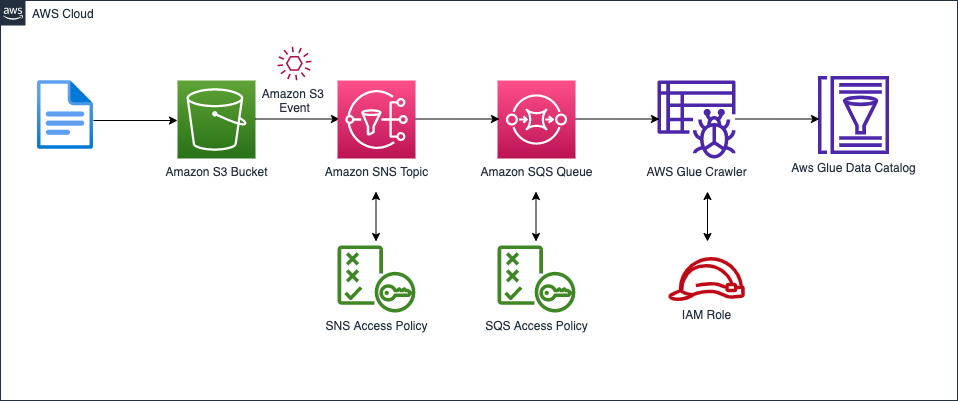
To accomplish incremental crawling, you can configure Amazon S3 Event Notifications to be sent to an Amazon Simple Queue Service (Amazon SQS) queue. You can then use the SQS queue as a source to identify changes and can schedule or run an AWS Glue crawler with Data Catalog tables as a target. With each run of the crawler, the SQS queue is inspected for new events. If no new events are found, the crawler stops. If events are found in the queue, the crawler inspects their respective folders, processes through built-in classifiers (for CSV, JSON, AVRO, XML, and so on), and determines the changes. The crawler then updates the Data Catalog with new information, such as newly added or deleted partitions or columns. This feature reduces the cost and time to crawl large and frequently changing Amazon S3 data.

This post shows how to create an AWS Glue crawler that supports Amazon S3 event notification on existing Data Catalog tables using the new crawler UI and an AWS CloudFormation template.

Overview of solution

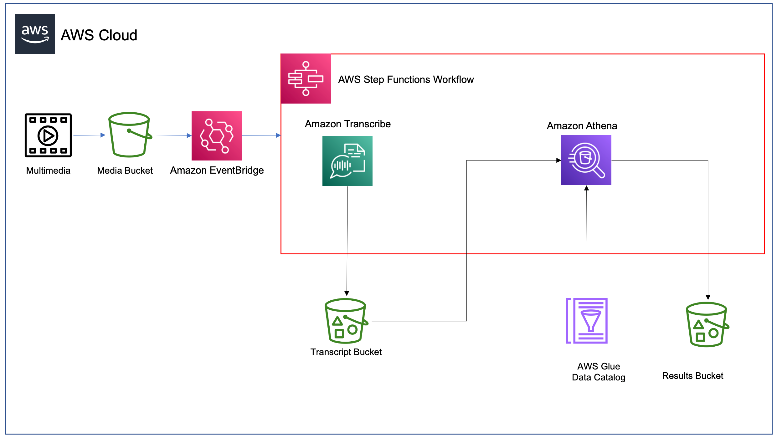
To demonstrate how the new AWS Glue crawler performs incremental updates, we use the Toronto parking tickets dataset—specifically data about parking tickets issued in the city of Toronto between 2019–2020. The goal is to create a manual dataset as well as its associated metadata tables in AWS Glue, followed by an event-based crawler that detects and implements changes to the manually created datasets and catalogs.

As mentioned before, instead of crawling all the subfolders on Amazon S3, we use an Amazon S3 event-based approach. This helps improve the crawl time by using Amazon S3 events to identify the changes between two crawls by listing all the files from the subfolder that triggered the event instead of listing the full Amazon S3 target. To accomplish this, we create an S3 bucket, an event-based crawler, an Amazon Simple Storage Service (Amazon SNS) topic, and an SQS queue. The following diagram illustrates our solution architecture.

Prerequisites

For this walkthrough, you should have the following prerequisites:

If the AWS account you use to follow this post uses Lake Formation to manage permissions on the AWS Glue Data Catalog, make sure that you log in as a user with access to create databases and tables. For more information, refer to Implicit Lake Formation permissions.

Launch your CloudFormation stack

To create your resources for this use case, complete the following steps:

  1. Launch your CloudFormation stack in us-east-1:
  2. For Stack name, enter a name for your stack .
  3. For paramBucketName, enter a name for your S3 bucket (with your account number).
  4. Choose Next.
  5. Select I acknowledge that AWS CloudFormation might create IAM resources with custom names.
  6. Choose Create stack.

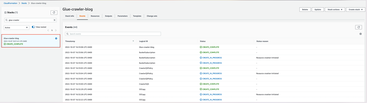
Wait for the stack formation to finish provisioning the requisite resources. When you see the CREATE_COMPLETE status, you can proceed to the next steps.

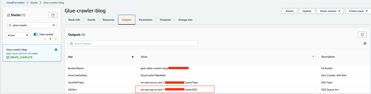
Additionally, note down the ARN of the SQS queue to use at a later point.

Query your Data Catalog

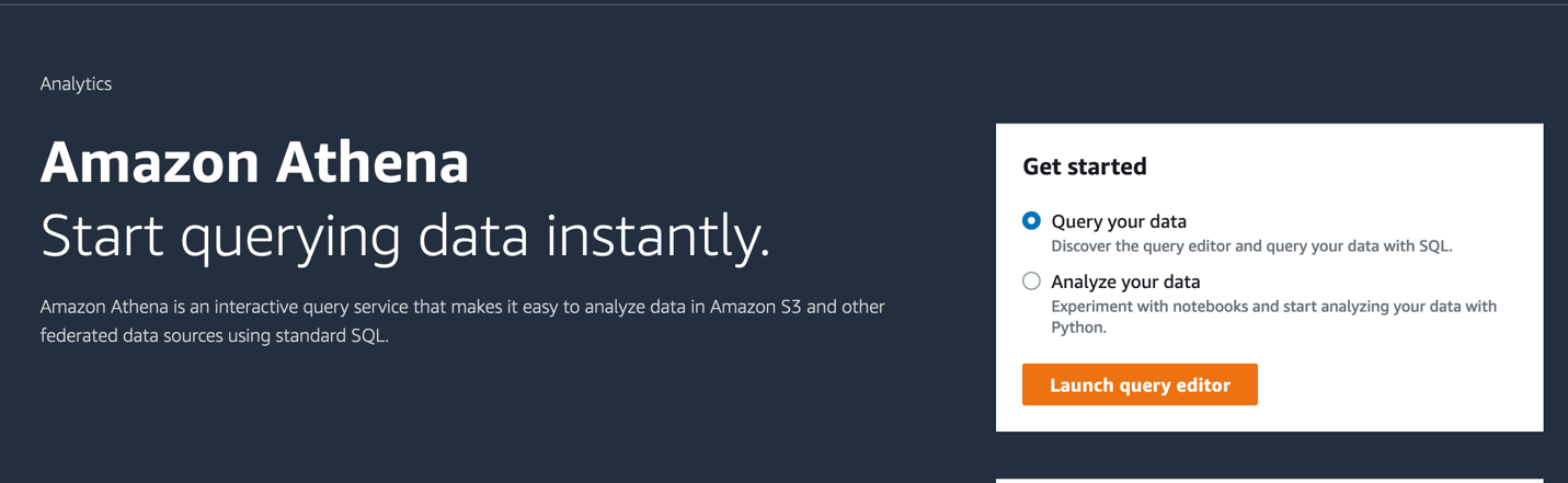
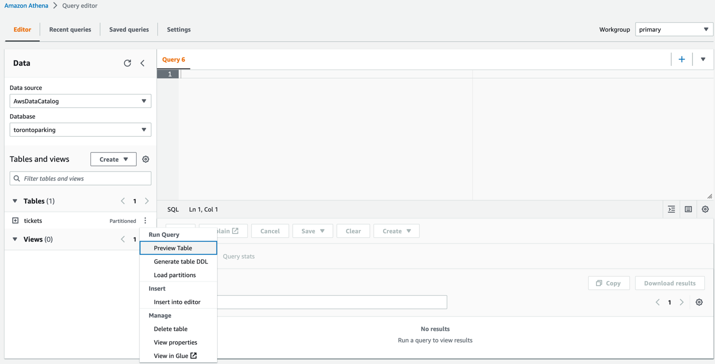
Next, we use Amazon Athena to confirm that the manual tables have been created in the Data Catalog, as part of the CloudFormation template.

  1. On the Athena console, choose Launch query editor.
  2. For Data source, choose AwsDataCatalog.
  3. For Database, choose torontoparking.

    The tickets table should appear in the Tables section.

    Now you can query the table to see its contents.
  4. You can write your own query, or choose Preview Table on the options menu.

    This writes a simple SQL query to show us the first 10 rows.
  5. Choose Run to run the query.

As we can see in the query results, the database and table for 2019 parking ticket data have been created and partitioned.

Create the Amazon S3 event crawler

The next step is to create the crawler that detects and crawls only on incrementally updated tables.

  1. On the AWS Glue console, choose Crawlers in the navigation pane.
  2. Choose Create crawler.
  3. For Name, enter a name.
  4. Choose Next.

    Now we need to select the data source for the crawler.
  5. Select Yes to indicate that our data is already mapped to our AWS Glue Data Catalog.
  6. Choose Add tables.
  7. For Database, choose torontoparking and for Tables, choose tickets.
  8. Select Crawl based on events.
  9. For Include SQS ARN, enter the ARN you saved from the CloudFormation stack outputs.
  10. Choose Confirm.

    You should now see the table populated under Glue tables, with the parameter set as Recrawl by event.
  11. Choose Next.
  12. For Existing IAM role, choose the IAM role created by the CloudFormation template (GlueCrawlerTableRole).
  13. Choose Next.
  14. For Frequency, choose On demand.

    You also have the option of choosing a schedule on which the crawler will run regularly.
  15. Choose Next.
  16. Review the configurations and choose Create crawler.

    Now that the crawler has been created, we add the 2020 ticketing data to our S3 bucket so that we can test our new crawler. For this step, we use the AWS Command Line Interface (AWS CLI)
  17. To add this data, use the following command:
    aws s3 cp s3://aws-bigdata-blog/artifacts/gluenewcrawlerui2/source/year=2020/Parking_Tags_Data_2020.000.csv s3://glue-table-crawler-blog-<YOURACCOUNTNUMBER>/year=2020/Parking_Tags_Data_2020.000.csv

After successful completion of this command, your S3 bucket should contain the 2020 ticketing data and your crawler is ready to run. The terminal should return the following:

copy: s3://aws-bigdata-blog/artifacts/gluenewcrawlerui2/source/year=2020/Parking_Tags_Data_2020.000.csv to s3://glue-table-crawler-blog-<YOURACCOUNTNUMBER>/year=2020/Parking_Tags_Data_2020.000.csvRun the crawler and verify the updates

Run the crawler and verify the updates

Now that the new folder has been created, we run the crawler to detect the changes in the table and partitions.

  1. Navigate to your crawler on the AWS Glue console and choose Run crawler.

    After running the crawler, you should see that it added the 2020 data to the tickets table.
  2. On the Athena console, we can ensure that the Data Catalog has been updated by adding a where year = 2020 filter to the query.

AWS CLI option

You can also create the crawler using the AWS CLI. For more information, refer to create-crawler.

Clean up

To avoid incurring future charges, and to clean up unused roles and policies, delete the resources you created: the CloudFormation stack, S3 bucket, AWS Glue crawler, AWS Glue database, and AWS Glue table.

Conclusion

You can use AWS Glue crawlers to discover datasets, extract schema information, and populate the AWS Glue Data Catalog. In this post, we provided a CloudFormation template to set up AWS Glue crawlers to use Amazon S3 event notifications on existing Data Catalog tables, which reduces the time and cost needed to incrementally process table data updates in the Data Catalog.

With this feature, incremental crawling can now be offloaded from data pipelines to the scheduled AWS Glue crawler, reducing cost. This alleviates the need for full crawls, thereby reducing crawl times and Data Processing Units (DPUs) required to run the crawler. This is especially useful for customers that have S3 buckets with event notifications enabled and want to continuously catalog new changes.

To learn more about this feature, refer to Accelerating crawls using Amazon S3 event notifications.

Special thanks to everyone who contributed to this crawler feature launch: Theo Xu, Jessica Cheng, Arvin Mohanty, and Joseph Barlan.


About the authors

Leonardo Gómez is a Senior Analytics Specialist Solutions Architect at AWS. Based in Toronto, Canada, he has over a decade of experience in data management, helping customers around the globe address their business and technical needs.

Aayzed Tanweer is a Solutions Architect working with startup customers in the FinTech space, with a special focus on analytics services. Originally hailing from Toronto, he recently moved to New York City, where he enjoys eating his way through the city and exploring its many peculiar nooks and crannies.

Sandeep Adwankar is a Senior Technical Product Manager at AWS. Based in the California Bay Area, he works with customers around the globe to translate business and technical requirements into products that enable customers to improve how they manage, secure, and access data.

AWS Week in Review – October 10, 2022

Post Syndicated from Marcia Villalba original https://aws.amazon.com/blogs/aws/aws-week-in-review-october-10-2022/

This post is part of our Week in Review series. Check back each week for a quick roundup of interesting news and announcements from AWS!

I had an amazing start to the week last week as I was speaking at the AWS Community Day NL. This event had 500 attendees and over 70 speakers, and Dr. Werner Vogels, Amazon CTO, delivered the keynote. AWS Community Days are community-led conferences organized by local communities, with a variety of workshops and sessions. I recommend checking your region for any of these events.

Community Day NL

Last Week’s Launches
Here are some launches that got my attention during the previous week.

Amazon S3 Object Lambda now supports using your own code to change the results of HEAD and LIST requests, besides GET (which we launched last year). This feature now enables more capabilities for what you can do with S3 Object Lambda. Danilo made a Twitter thread with lots of use cases for this new launch.

Amazon SageMaker Clarify now can provide near real-time explanations for ML predictions. SageMaker Clarify is a service that provides explainability by ML models individual predictions. These explanations are important for developers to get visibility into their training data and models to identify potential bias.

AWS Storage Gateway now supports 15 TiB tapes. It increased the maximum supported virtual tape size on Tape Gateway from 5 TiB to 15 TiB, so you can store more data on a single virtual tape, and you can reduce the number of tapes you need to manage.

Amazon Aurora Serverless v2 now supports AWS CloudFormation. Early this year, we announced the general availability of Aurora Serverless v2, and now you can use AWS CloudFormation Templates to deploy and change the database along with the rest of your infrastructure.

AWS Config now supports 15 new resource types, including AWS DataSync, Amazon GuardDuty, Amazon Simple Email Service (Amazon SES), AWS AppSync, AWS Cloud Map, Amazon EC2, and AWS AppConfig. With this launch, you can use AWS Config to monitor configuration data for the supported resource types in your AWS account, and you can see how the configuration changes.

For a full list of AWS announcements, be sure to keep an eye on the What’s New at AWS page.

Other AWS News
Some other updates and news that you may have missed:

This week an article about how AWS is leading a pilot project to turn the Greek island of Naxos into a smart island caught my attention. The project introduces smart solutions for mobility, primary healthcare, and the transport of goods. The solution has been built based on four pillars that were important for the island: sustainability, telehealth, leisure, and digital skills. Check out the whole article to learn what they are doing.

Podcast Charlas Técnicas de AWS – If you understand Spanish, this podcast is for you. Podcast Charlas Técnicas is one of the official AWS podcasts in Spanish, and every other week there is a new episode. The podcast is meant for builders, and it shares stories about how customers implemented and learned AWS services, how to architect applications, and how to use new services. You can listen to all the episodes directly from your favorite podcast app or at AWS Podcasts en español.

AWS open-source news and updates – This is a newsletter curated by my colleague Ricardo to bring you the latest open-source projects, posts, events, and more.

Upcoming AWS Events
Check your calendars and sign up for these AWS events:

AWS re:Invent reserved seating opens on October 11. If you are planning to attend, book a spot in advance for your favorite sessions. AWS re:Invent is our biggest conference of the year, it happens in Las Vegas from November 28 to December 2, and registrations are open. Many writers of this blog have sessions at re:Invent, and you can search the event agenda using our names.

I started the post talking about AWS Community Days, and there is one in Warsaw, Poland, on October 14. If you are around Warsaw during this week, you can first check out the AWS Pop-up Hub in Warsaw that runs October 10-14 and then join for the Community Day.

On October 20, there is a virtual event for modernizing .NET workloads with Windows containers on AWS, You can register for free.

That’s all for this week. Check back next Monday for another Week in Review!

— Marcia

Lifting and shifting a web application to AWS Serverless: Part 2

Post Syndicated from Marcia Villalba original https://aws.amazon.com/blogs/compute/lifting-and-shifting-a-web-application-to-aws-serverless-part-2/

In part 1, you learn if it is possible to migrate a non-serverless web application to a serverless environment without changing much code. You learn different tools that can help you in this process, like Lambda Web Adaptor and AWS Amplify. By the end, you have migrated an application into a serverless environment.

However, if you test the migrated app, you find two issues. The first one is that the user session is not sticky. Every time you log in, you are logged out unexpectedly from the application. The second one is that when you create a new product, you cannot upload new images of that product.

This final post analyzes each of the problems in detail and shows solutions. In addition, it analyzes the cost and performance of the solution.

Authentication and authorization migration

The original application handled the authentication and authorization by itself. There is a user directory in the database, with the passwords and emails for each of the users. There are APIs and middleware that take care of validating that the user is logged in before showing the application. All the logic for this is developed inside the Node.js/Express application.

However, with the current migrated application every time you log in, you are logged out unexpectedly from the application. This is because the server code is responsible for handling the authentication and the authorization of the users, and now our server is running in an AWS Lambda function and functions are stateless. This means that there will be one function running per request—a request can load all the products in the landing page, get the details for a product, or log in to the site—and if you do something in one of these functions, the state is not shared across.

To solve this, you must remove the authentication and authorization mechanisms from the function and use a service that can preserve the state across multiple invocations of the functions.

There are many ways to solve this challenge. You can add a layer of authentication and session management with a database like Redis, or build a new microservice that is in charge of authentication and authorization that can handle the state, or use an existing managed service for this.

Because of the migration requirements, we want to keep the cost as low as possible, with the fewest changes to the application. The better solution is to use an existing managed service to handle authentication and authorization.

This demo uses Amazon Cognito, which provides user authentication and authorization to AWS resources in a managed, pay as you go way. One rapid approach is to replace all the server code with calls to Amazon Cognito using the AWS SDK. But this adds complexity that can be replaced completely by just invoking Amazon Cognito APIs from the React application.

Using Cognito

For example, when a new user is registered, the application creates the user in the Amazon Cognito user pool directory, as well as in the application database. But when a user logs in to the web app, the application calls Amazon Cognito API directly from the AWS Amplify application. This way minimizes the amount of code needed.

In the original application, all authenticated server APIs are secured with a middleware that validates that the user is authenticated by providing an access token. With the new setup that doesn’t change, but the token is generated by Amazon Cognito and then it can be validated in the backend.

let auth = (req, res, next) => {
    const token = req.headers.authorization;
    const jwtToken = token.replace('Bearer ', '');

    verifyToken(jwtToken)
        .then((valid) => {
            if (valid) {
                getCognitoUser(jwtToken).then((email) => {
                    User.findByEmail(email, (err, user) => {
                        if (err) throw err;
                        if (!user)
                            return res.json({
                                isAuth: false,
                                error: true,
                            });

                        req.user = user;
                        next();
                    });
                });
            } else {
                throw Error('Not valid Token');
            }
        })
        .catch((error) => {
            return res.json({
                isAuth: false,
                error: true,
            });
        });
};

You can see how this is implemented step by step in this video.

Storage migration

In the original application, when a new product is created, a new image is uploaded to the Node.js/Express server. However, now the application resides in a Lambda function. The code (and files) that are part of that function cannot change, unless the function is redeployed. Consequently, you must separate the user storage from the server code.

For doing this, there are a couple of solutions: using Amazon Elastic File System (EFS) or Amazon S3. EFS is a file storage, and you can use that to have a dynamic storage where you upload the new images. Using EFS won’t change much of the code, as the original implementation is using a directory inside the server as EFS provides. However, using EFS adds more complexity to the application, as functions that use EFS must be inside an Amazon Virtual Private Cloud (Amazon VPC).

Using S3 to upload your images to the application is simpler, as it only requires that an S3 bucket exists. For doing this, you must refactor the application, from uploading the image to the application API to use the AWS Amplify library that uploads and gets images from S3.

export function uploadImage(file) {
    const fileName = `uploads/${file.name}`;

    const request = Storage.put(fileName, file).then((result) => {
        return {
            image: fileName,
            success: true,
        };
    });

    return {
        type: IMAGE_UPLOAD,
        payload: request,
    };
}

An important benefit of using S3 is that you can also use Amazon CloudFront to accelerate the retrieval of the images from the cloud. In this way, you can speed up the loading time of your page. You can see how this is implemented step by step in this video.

How much does this application cost?

If you deploy this application in an empty AWS account, most of the usage of this application is covered by the AWS Free Tier. Serverless services, like Lambda and Amazon Cognito, have a forever free tier that gives you the benefits in pricing for the lifetime of hosting the application.

  • AWS Lambda—With 100 requests per hour, an average 10ms invocation and 1GB of memory configured, it costs 0 USD per month.
  • Amazon S3—Using S3 standard, hosting 1 GB per month and 10k PUT and GET requests per month costs 0.07 USD per month. This can be optimized using S3 Intelligent-Tiering.
  • Amazon Cognito—Provides 50,000 monthly active users for free.
  • AWS Amplify—If you build your client application once a week, serve 3 GB and store 1 GB per month, this costs 0.87 USD.
  • AWS Secrets Manager—There are two secrets stored using Secrets Manager and this costs 1.16 USD per month. This can be optimized by using AWS System Manager Parameter Store and AWS Key Management Service (AWS KMS).
  • MongoDB Atlas Forever free shared cluster.

The total monthly cost of this application is approximately 2.11 USD.

Performance analysis

After you migrate the application, you can run a page speed insight tool, to measure this application’s performance. This tool provides results mostly about the front end and the experience that the user perceives. The results are displayed in the following image. The performance of this website is good, according to the insight tool performance score – it responds quickly and the user experience is good.

Page speed insight tool results

After the application is migrated to a serverless environment, you can do some refactoring to improve further the overall performance. One alternative is whenever a new image is uploaded, it gets resized and formatted into the correct next-gen format automatically using the event driven capabilities that S3 provides. Another alternative is to use Lambda on Edge to serve the right image size for the device, as it is possible to format the images on the fly when serving them from a distribution.

You can run load tests for understanding how your backend and database will perform. For this, you can use Artillery, an open-source library that allows you to run load tests. You can run tests with the expected maximum load your site will get and ensure that your site can handle it.

For example, you can configure a test that sends 30 requests per seconds to see how your application reacts:

config:
  target: 'https://xxx.lambda-url.eu-west-1.on.aws'
  phases:
    - duration: 240
      arrivalRate: 30
      name: Testing
scenarios:
  - name: 'Test main page'
    flow:
      - post:
          url: '/api/product/getProducts/'

This test is performed on the backend APIs, not only testing your backend but also your integration with the MongoDB. After running it, you can see how the Lambda function performs on the Amazon CloudWatch dashboard.

Running this load test helps you understand the limitations of your system. For example, if you run a test with too many concurrent users, you might see that the number of throttles in your function increases. This means that you need to lift the limit of invocations of the functions you can have at the same time.

Or when increasing the requests per second, you may find that the MongoDB cluster starts throttling your requests. This is because you are using the free tier and that has a set number of connections. You might need a larger cluster or to migrate your database to another service that provides a large free tier, like Amazon DynamoDB.

Cloudwatch dashboard

Conclusion

In this two-part article, you learn if it is possible to migrate a non-serverless web application to a serverless environment without changing much code. You learn different tools that can help you in this process, like AWS Lambda Web Adaptor and AWS Amplify, and how to solve some of the typical challenges that we have, like storage and authentication.

After the application is hosted in a fully serverless environment, it can scale up and down to meet your needs. This web application is also performant once the backend is hosted in a Lambda function.

If you need, from here you can start using the strangler pattern to refactor the application to take advantage of the benefits of event-driven architecture.

To see all the steps of the migration, there is a playlist that contains all the tutorials for you to follow.

For more serverless learning resources, visit Serverless Land.

Lifting and shifting a web application to AWS Serverless: Part 1

Post Syndicated from Marcia Villalba original https://aws.amazon.com/blogs/compute/lifting-and-shifting-a-web-application-to-aws-serverless-part-1/

Customers migrating to the cloud often want to get the benefits of serverless architecture. But what is the best approach and is it possible? There are many strategies to do a migration, but lift and shift is often the fastest way to get to production with the migrated workload.

You might also wonder if it’s possible to lift and shift an existing application that runs in a traditional environment to serverless. This blog post shows how to do this for a Mongo, Express, React, and Node.js (MERN) stack web app. However, the discussions presented in this post apply to other stacks too.

Why do a lift and shift migration?

Lift and shift, or sometimes referred to as rehosting the application, is moving the application with as few changes as possible. Lift and shift migrations often allow you to get the new workload in production as fast as possible. When migrating to serverless, lift and shift can bring a workload that is not yet in the cloud or in a serverless environment to use managed and serverless services quickly.

Migrating a non-serverless workload to serverless with lift and shift might not bring all the serverless benefits right away, but it enables the development team to refactor, using the strangler pattern, the parts of the application that might benefit from what serverless technologies offer.

Why migrate a web app to serverless?

Web apps hosted in a serverless environment benefit most from the capability of serverless applications to scale automatically and for paying for what you use.

Imagine that you have a personal web app with little traffic. If you are hosting in a serverless environment, you don’t pay a fixed price to have the servers up and running. Your web app has only a few requests and the rest of the time is idle.

This benefit applies to the opposite case. For an owner of a small ecommerce site running on a server, imagine if a social media influencer with millions of followers recommends one of their products. Suddenly, thousands of requests arrive and make the site unavailable. If the site is hosted on a serverless platform, the application will scale to the traffic that it receives.

Requirements for migration

Before starting a migration, it is important to define the nonfunctional requirements that you need the new application to have. These requirements help when you must make architectural decisions during the migration process.

These are the nonfunctional requirements of this migration:

  • Environment that scales to zero and scales up automatically.
  • Pay as little as possible for idle time.
  • Configure as little infrastructure as possible.
  • Automatic high availability of the application.
  • Minimal changes to the original code.

Application overview

This blog post guides you on how to migrate a MERN application. The original application is hosted in two different servers: One contains the Mongo database and another contains the Node/js/Express and ReactJS applications.

Application overview

This demo application simulates a swag ecommerce site. The database layer stores the products, users, and the purchases history. The server layer takes care of the ecommerce business logic, hosting the product images, and user authentication and authorization. The web layer takes care of all the user interaction and communicates with the server layer using REST APIs.

How the application looks like

These are the changes that you must make to migrate to a serverless environment:

  • Database migration: Migrate the database from on-premises to MongoDB Atlas.
  • Backend migration: Migrate the NodeJS/Express application from on-premises to an AWS Lambda function.
  • Web app migration: Migrate the React web app from on-premises to AWS Amplify.
  • Authentication migration: Migrate the custom-built authentication to use Amazon Cognito.
  • Storage migration: Migrate the local storage of images to use Amazon S3 and Amazon CloudFront.

The following image shows the proposed solution for the migrated application:

Proposed architecture

Database migration

The database is already in a MongoDB vanilla container that has all the data for this application. As MongoDB is the database engine for our stack, their recommended solution to migrate to serverless is to use MongoDB Atlas. Atlas provides a database cluster in the cloud that scales automatically and you pay for what you use.

To get started, create a new Atlas cluster, then migrate the data from the existing database to the serverless one. To migrate the data, you can first dump all the content of the database to a dump folder and then restore it to the cloud:

mongodump --uri="mongodb://<localuser>:<localpassword>@localhost:27017"

mongorestore --uri="mongodb+srv://<user>:<password>@<clustername>.debkm.mongodb.net" .

After doing that, your data is now in the cloud. The next step is to change the configuration string in the server to point to the new database. To see this in action, check this video that shows a walkthrough of the migration.

Backend migration

Migrating the Node.js/Express backend is the most challenging of the layers to migrate to a serverless environment, as the server layer is a Node.js application that runs in a server.

One option for this migration is to use AWS Fargate. Fargate is a serverless container service that allows you to scale automatically and you pay as you go. Another option is to use AWS AppRunner, a container service that auto scales and you also pay as you go. However, neither of these options align with our migration requirements, as they don’t scale to zero.

Another option for the lift and shift migration of this Node.js application is to use Lambda with the AWS Lambda Web Adapter. The AWS Lambda Web Adapter is an open-source project that allows you to build web applications with familiar frameworks, like Express.js, Flask, SpringBoot, and run it on Lambda. You can learn more about this project in its GitHub repository.

Lambda Web Adapter

Using this project, you can create a new Lambda function that has the Express/NodeJS application as the function code. You can lift and shift all the code into the function. If you want a step-by-step tutorial on how to do this, check out this video.

const lambdaAdapterFunction = new Function(this,`${props.stage}-LambdaAdapterFunction`,
            {
                runtime: Runtime.NODEJS_16_X,
                code: Code.fromAsset('backend-app'),
                handler: 'run.sh',
                environment: {
                    AWS_LAMBDA_EXEC_WRAPPER: '/opt/bootstrap',
                    REGION: this.region,
                    ASYNC_INIT: 'true',
                },
                memorySize: 1024,
                layers: [layerLambdaAdapter],
                timeout: Duration.seconds(2),
                tracing: Tracing.ACTIVE,
            }
        );

The next step is to create an HTTP endpoint for the server application. There are three options for doing this: API Gateway, Application Load Balancer (ALB) , or to use Lambda Function URLs. All the options are compatible with Lambda Web Adapter and can solve the challenge for you.

For this demo, choose function URLs, as they are simple to configure and one function URL forwards all routes to the Express server. API Gateway and ALB require more configuration and have separate costs, while the cost of function URLs is included in the Lambda function.

Web app migration

The final layer to migrate is the React application. The best way to migrate the web layer and to adhere to the migration requirements is to use AWS Amplify to host it. AWS Amplify is a fully managed service that provides many features like hosting web applications and managing the CICD process for the web app. It provides client libraries to connect to different AWS resources, and many other features.

Migrating the React application is as simple as creating a new Amplify application in your AWS account and uploading the React application to a code repository like GitHub. This AWS Amplify application is connected to a GitHub branch, and when there is a new commit in this branch, AWS Amplify redeploys the code.

The Amplify application receives configuration parameters like the function URL endpoint (the server URL) using environmental variables.

const amplifyApp = new App(this, `${props.stage}-AmplifyReactShopApp`, {
            sourceCodeProvider: new GitHubSourceCodeProvider({
                owner: config.frontend.owner,
                repository: config.frontend.repository_name,
                oauthToken: SecretValue.secretsManager('github-token'),
            }),
            environmentVariables: {
                REGION: this.region,
                SERVER_URL: props.serverURL,
            },
        });

If you want to see a step-by-step guide on how to make your web layer serverless, you can check this video.

Next steps

However, if you test this migrated app, you will find two issues. The first one is that the user session is not sticky. Every time you log in, you are logged out unexpectedly from the application. The second one is that when you create a new product, you cannot upload new images of that product.

In part two, I analyze each of the problems in detail and find solutions. These issues arise because of the stateless and immutable characteristics of this solution. The next part of this article explains how to solve these issues, also it analyzes costs and performance of the solution.

Conclusion

In this article, you learn if it is possible to migrate a non-serverless web application to a serverless environment without changing much code. You learn different tools that can help you in this process, like the AWS Lambda Web Adaptor and AWS Amplify.

If you want to see the migration in action and learn all the steps for this, there is a playlist that contains all the tutorials for you to follow and learn how this is possible.

For more serverless learning resources, visit Serverless Land.

Convert Oracle XML BLOB data to JSON using Amazon EMR and load to Amazon Redshift

Post Syndicated from Abhilash Nagilla original https://aws.amazon.com/blogs/big-data/convert-oracle-xml-blob-data-to-json-using-amazon-emr-and-load-to-amazon-redshift/

In legacy relational database management systems, data is stored in several complex data types, such XML, JSON, BLOB, or CLOB. This data might contain valuable information that is often difficult to transform into insights, so you might be looking for ways to load and use this data in a modern cloud data warehouse such as Amazon Redshift. One such example is migrating data from a legacy Oracle database with XML BLOB fields to Amazon Redshift, by performing preprocessing and conversion of XML to JSON using Amazon EMR. In this post, we describe a solution architecture for this use case, and show you how to implement the code to handle the XML conversion.

Solution overview

The first step in any data migration project is to capture and ingest the data from the source database. For this task, we use AWS Database Migration Service (AWS DMS), a service that helps you migrate databases to AWS quickly and securely. In this example, we use AWS DMS to extract data from an Oracle database with XML BLOB fields and stage the same data in Amazon Simple Storage Service (Amazon S3) in Apache Parquet format. Amazon S3 is an object storage service offering industry-leading scalability, data availability, security, and performance, and is the storage of choice for setting up data lakes on AWS.

After the data is ingested into an S3 staging bucket, we used Amazon EMR to run a Spark job to perform the conversion of XML fields to JSON fields, and the results are loaded in a curated S3 bucket. Amazon EMR runtime for Apache Spark can be over three times faster than clusters without EMR runtime, and has 100% API compatibility with standard Apache Spark. This improved performance means your workloads run faster and it saves you compute costs, without making any changes to your application.

Finally, transformed and curated data is loaded into Amazon Redshift tables using the COPY command. The Amazon Redshift table structure should match the number of columns and the column data types in the source file. Because we stored the data as a Parquet file, we specify the SERIALIZETOJSON option in the COPY command. This allows us to load complex types, such as structure and array, in a column defined as SUPER data type in the table.

The following architecture diagram shows the end-to-end workflow.

In detail, AWS DMS migrates data from the source database tables into Amazon S3, in Parquet format. Apache Spark on Amazon EMR reads the raw data, transforms the XML data type into JSON, and saves the data to the curated S3 bucket. In our code, we used an open-source library, called spark-xml, to parse and query the XML data.

In the rest of this post, we assume that the AWS DMS tasks have already run and created the source Parquet files in the S3 staging bucket. If you want to set up AWS DMS to read from an Oracle database with LOB fields, refer to Effectively migrating LOB data to Amazon S3 from Amazon RDS for Oracle with AWS DMS or watch the video Migrate Oracle to S3 Data lake via AWS DMS.

Prerequisites

If you want to follow along with the examples in this post using your AWS account, we provide an AWS CloudFormation template you can launch by choosing Launch Stack:

BDB-2063-launch-cloudformation-stack

Provide a stack name and leave the default settings for everything else. Wait for the stack to display Create Complete (this should only take a few minutes) before moving on to the other sections.

The template creates the following resources:

  • A virtual private cloud (VPC) with two private subnets that have routes to an Amazon S3 VPC endpoint
  • The S3 bucket {stackname}-s3bucket-{xxx}, which contains the following folders:
    • libs – Contains the JAR file to add to the notebook
    • notebooks – Contains the notebook to interactively test the code
    • data – Contains the sample data
  • An Amazon Redshift cluster, in one of the two private subnets, with a database named rs_xml_db and a schema named rs_xml
  • A secret (rs_xml_db) in AWS Secrets Manager
  • An EMR cluster

The CloudFormation template shared in this post is purely for demonstration purposes only. Please conduct your own security review and incorporate best practices prior to any production deployment using artifacts from the post.

Finally, some basic knowledge of Python and Spark DataFrames can help you review the transformation code, but isn’t mandatory to complete the example.

Understanding the sample data

In this post, we use college students’ course and subjects sample data that we created. In the source system, data consists of flat structure fields, like course_id and course_name, and an XML field that includes all the course material and subjects involved in the respective course. The following screenshot is an example of the source data, which is staged in an S3 bucket as a prerequisite step.

We can observe that the column study_material_info is an XML type field and contains nested XML tags in it. Let’s see how to convert this nested XML field to JSON in the subsequent steps.

Run a Spark job in Amazon EMR to transform the XML fields in the raw data to JSON

In this step, we use an Amazon EMR notebook, which is a managed environment to create and open Jupyter Notebook and JupyterLab interfaces. It enables you to interactively analyze and visualize data, collaborate with peers, and build applications using Apache Spark on EMR clusters. To open the notebook, follow these steps:

  1. On the Amazon S3 console, navigate to the bucket you created as a prerequisite step.
  2. Download the file in the notebooks folder.
  3. On the Amazon EMR console, choose Notebooks in the navigation pane.
  4. Choose Create notebook.
  5. For Notebook name, enter a name.
  6. For Cluster, select Choose an existing cluster.
  7. Select the cluster you created as a prerequisite.
  8. For Security Groups, choose BDB1909-EMR-LIVY-SG and BDB1909-EMR-Notebook-SG
  9. For AWS Service Role, choose the role bdb1909-emrNotebookRole-{xxx}.
  10. For Notebook location, specify the S3 path in the notebooks folder (s3://{stackname}-s3bucket-xxx}/notebooks/).
  11. Choose Create notebook.
  12. When the notebook is created, choose Open in JupyterLab.
  13. Upload the file you downloaded earlier.
  14. Open the new notebook.

    The notebook should look as shown in the following screenshot, and it contains a script written in Scala.
  15. Run the first two cells to configure Apache Spark with the open-source spark-xml library and import the needed modules.The spark-xml package allows reading XML files in local or distributed file systems as Spark DataFrames. Although primarily used to convert (portions of) large XML documents into a DataFrame, spark-xml can also parse XML in a string-valued column in an existing DataFrame with the from_xml function, in order to add it as a new column with parsed results as a struct.
  16. To do so, in the third cell, we load the data from the Parquet file generated by AWS DMS into a DataFrame, then we extract the attribute that contains the XML code (STUDY_MATERIAL_INFO) and map it to a string variable name payloadSchema.
  17. We can now use the payloadSchema in the from_xml function to convert the field STUDY_MATERIAL_INFO into a struct data type and added it as a column named course_material in a new DataFrame parsed.
  18. Finally, we can drop the original field and write the parsed DataFrame to our curated zone in Amazon S3.

Due to the structure differences between DataFrame and XML, there are some conversion rules from XML data to DataFrame and from DataFrame to XML data. More details and documentation are available XML Data Source for Apache Spark.

When we convert from XML to DataFrame, attributes are converted as fields with the heading prefix attributePrefix (underscore (_) is the default). For example, see the following code:

  <book category="undergraduate">
    <title lang="en">Introduction to Biology</title>
    <author>Demo Author 1</author>
    <year>2005</year>
    <price>30.00</price>
  </book>

It produces the following schema:

root
 |-- category: string (nullable = true)
 |-- title: struct (nullable = true)
 |    |-- _VALUE: string (nullable = true)
 |    |-- _lang: string (nullable = true)
 |-- author: string (nullable = true)
 |-- year: string (nullable = true)
 |-- price: string (nullable = true)

Next, we have a value in an element that has no child elements but attributes. The value is put in a separate field, valueTag. See the following code:

<title lang="en">Introduction to Biology</title>

It produces the following schema, and the tag lang is converted into the _lang field inside the DataFrame:

|-- title: struct (nullable = true)
 |    |-- _VALUE: string (nullable = true)
 |    |-- _lang: string (nullable = true)

Copy curated data into Amazon Redshift and query tables seamlessly

Because our semi-structured nested dataset is already written in the S3 bucket as Apache Parquet formatted files, we can use the COPY command with the SERIALIZETOJSON option to ingest data into Amazon Redshift. The Amazon Redshift table structure should match the metadata of the Parquet files. Amazon Redshift can replace any Parquet columns, including structure and array types, with SUPER data columns.

The following code demonstrates CREATE TABLE example to create a staging table.

create table rs_xml_db.public.stg_edw_course_catalog 
(
course_id bigint,
course_name character varying(5000),
course_material super
);

The following code uses the COPY example to load from Parquet format:

COPY rs_xml_db.public.stg_edw_course_catalog FROM 's3://<<your Amazon S3 Bucket for curated data>>/data/target/<<your output parquet file>>' 
IAM_ROLE '<<your IAM role>>' 
FORMAT PARQUET SERIALIZETOJSON; 

By using semistructured data support in Amazon Redshift, you can ingest and store semistructured data in your Amazon Redshift data warehouses. With the SUPER data type and PartiQL language, Amazon Redshift expands the data warehouse capability to integrate with both SQL and NoSQL data sources. The SUPER data type only supports up to 1 MB of data for an individual SUPER field or object. Note, the JSON object may be stored in a SUPER data type, but reading this data using JSON functions currently has a VARCHAR (65535 byte) limit. See Limitations for more details.

The following example shows how nested JSON can be easily accessed using SELECT statements:

SELECT DISTINCT bk._category
	,bk.author
	,bk.price
	,bk.year
	,bk.title._lang
FROM rs_xml_db.public.stg_edw_course_catalog main
INNER JOIN main.course_material.book bk ON true;

The following screenshot shows our results.

Clean up

To avoid incurring future charges, first delete the notebook and the related files on Amazon S3 bucket as explained in this EMR documentation page then the CloudFormation stack.

Conclusion

This post demonstrated how to use AWS services like AWS DMS, Amazon S3, Amazon EMR, and Amazon Redshift to seamlessly work with complex data types like XML and perform historical migrations when building a cloud data lake house on AWS. We encourage you to try this solution and take advantage of all the benefits of these purpose-built services.

If you have questions or suggestions, please leave a comment.


About the authors

Abhilash Nagilla is a Sr. Specialist Solutions Architect at AWS, helping public sector customers on their cloud journey with a focus on AWS analytics services. Outside of work, Abhilash enjoys learning new technologies, watching movies, and visiting new places.

Avinash Makey is a Specialist Solutions Architect at AWS. He helps customers with data and analytics solutions in AWS. Outside of work he plays cricket, tennis and volleyball in free time.

Fabrizio Napolitano is a Senior Specialist SA for DB and Analytics. He has worked in the analytics space for the last 20 years, and has recently and quite by surprise become a Hockey Dad after moving to Canada.

A multi-dimensional approach helps you proactively prepare for failures, Part 2: Infrastructure layer

Post Syndicated from Piyali Kamra original https://aws.amazon.com/blogs/architecture/a-multi-dimensional-approach-helps-you-proactively-prepare-for-failures-part-2-infrastructure-layer/

Distributed applications resiliency is a cumulative resiliency of applications, infrastructure, and operational processes. Part 1 of this series explored application layer resiliency. In Part 2, we discuss how using Amazon Web Services (AWS) managed services, redundancy, high availability, and infrastructure failover patterns based on recovery time and point objectives (RTO and RPO, respectively) can help in building more resilient infrastructures.

Pattern 1: Recognize high impact/likelihood infrastructure failures

To ensure cloud infrastructure resilience, we need to understand the likelihood and impact of various infrastructure failures, so we can mitigate them. Figure 1 illustrates that most of the failures with high likelihood happen because of operator error or poor deployments.

Automated testing, automated deployments, and solid design patterns can mitigate these failures. There could be datacenter failures—like whole rack failures—but deploying applications using auto scaling and multi-availability zone (multi-AZ) deployment, plus resilient AWS cloud native services, can mitigate the impact.

Likelihood and impact of failure events

Figure 1. Likelihood and impact of failure events

As demonstrated in the Figure 1, infrastructure resiliency is a combination of high availability (HA) and disaster recovery (DR). HA involves increasing the availability of the system by implementing redundancy among the application components and removing single points of failure.

Application layer decisions, like creating stateless applications, make it simpler to implement HA at the infrastructure layer by allowing it to scale using Auto Scaling groups and distributing the redundant applications across multiple AZs.

Pattern 2: Understanding and controlling infrastructure failures

Building a resilient infrastructure requires understanding which infrastructure failures are under control and which ones are not, as demonstrated in Figure 2.

These insights allow us to automate the detection of failures, control them, and employ pro-active patterns, such as static stability, to mitigate the need to scale up the infrastructure by over-provisioning it in advance.

Proactively designing systems in the event of failure

Figure 2. Proactively designing systems in the event of failure

The infrastructure decisions under our control that can increase the infrastructure resiliency of our system, include:

  • AWS services have control and data planes designed for minimum blast radius. Data planes typically have higher availability design goals than control planes and are usually less complex. When implementing recovery or mitigation responses to events that can affect resiliency, using control plane operations can lower the overall resiliency of your architectures. For example, Amazon Route 53 (Route 53) has a data plane designed for a 100% availability SLA. A good fail-over mechanism should rely on the data plane and not the control plane, as explained in Creating Disaster Recovery Mechanisms Using Amazon Route 53.
  • Understanding networking design and routes implemented in a virtual private cloud (VPC) are critical when testing the flow of traffic in our application. Understanding the flow of traffic helps us design better applications and see how one component failure can affect overall ingress/egress traffic. To achieve better network resiliency, it’s important to implement a good subnet strategy and manage our IP addresses to avoid fail-over issues and asymmetric routing in hybrid architectures. Use IP address management tools for established subnet strategies and routing decisions.
  • When designing VPCs and AZs, understanding the service limits, deploying independent routing tables and components in each zone increases availability. For example, highly available NAT gateways are preferred over NAT instances, as noted in the comparison provided in the Amazon VPC documentation.

Pattern 3: Considering different ways of increasing HA at the infrastructure layer

As already detailed, infrastructure resiliency = HA + DR.

Different ways by which system availability can be increased include:

  • Building for redundancy: Redundancy is the duplication of application components to increase the overall availability of the distributed system. After following application layer best practices, we can build auto healing mechanisms at the infrastructure layer.

We can take advantage of auto scaling features and use Amazon CloudWatch metrics and alarms to set up auto scaling triggers and deploy redundant copies of our applications across multiple AZs. This protects workloads from AZ failures, as shown in Figure 3.

Redundancy increases availability

Figure 3. Redundancy increases availability

  • Auto scale your infrastructure: When there are AZ failures, infrastructure auto scaling maintains the desired number of redundant components, which helps maintain the base level application throughput. This way, HA system and manage costs are maintained. Auto scaling uses metrics to scale in and out, appropriately, as shown in Figure 4.
How auto scaling improves availability

Figure 4. How auto scaling improves availability

  • Implement resilient network connectivity patterns: While building highly resilient distributed systems, network access to AWS infrastructure also needs to be highly resilient. While deploying hybrid applications, the capacity needed for hybrid applications to communicate with their cloud native application counterparts is an important consideration in designing the network access using AWS Direct Connect or VPNs.

Testing failover and fallback scenarios helps validate that network paths operate as expected and routes fail over as expected to meet RTO objectives. As the number of connection points between the data center and AWS VPCs increases, a hub and spoke configuration provided by the Direct Connect gateway and transit gateways simplify network topology, testing, and fail over. For more information, visit the AWS Direct Connect Resiliency Recommendations.

  • Whenever possible, use the AWS networking backbone to increase security, resiliency, and lower cost. AWS PrivateLink provides secure access to AWS services and exposes the application’s functionalities and APIs to other business units or partner accounts hosted on AWS.
  • Security appliances need to be set up in HA configuration, so that even if one AZ is unavailable, security inspection can be taken over by the redundant appliances in the other AZs.
  • Think ahead about DNS resolution: DNS is a critical infrastructure component; hybrid DNS resolution should be designed carefully with Route 53 HA inbound and outbound resolver endpoints instead of using self-managed proxies.

Implement a good strategy to share DNS resolver rules across AWS accounts and VPC’s with Resource Access Manager. Network failover tests are an important part of Disaster Recovery and Business Continuity Plans. To learn more, visit Set up integrated DNS resolution for hybrid networks in Amazon Route 53.

Additionally, ELB uses health checks to make sure that requests will route to another component if the underlying traffic application component fails. This improves the distributed system’s availability, as it is the cumulative availability of all different layers in our system. Figure 5 details advantages of some AWS managed services.

AWS managed services help in building resilient infrastructures (click the image to enlarge)

Figure 5. AWS managed services help in building resilient infrastructures (click the image to enlarge)

Pattern 4: Use RTO and RPO requirements to determine the correct failover strategy for your application

Capture RTO and RPO requirements early on to determine solid failover strategies (Figure 6). Disaster recovery strategies within AWS range from low cost and complexity (like backup and restore), to more complex strategies when lower values of RTO and RPO are required.

In pilot light and warm standby, only the primary region receives traffic. Pilot light only critical infrastructure components run in the backup region. Automation is used to check failures in the primary region using health checks and other metrics.

When health checks fail, use a combination of auto scaling groups, automation, and Infrastructure as Code (IaC) for quick deployment of other infrastructure components.

Note: This strategy depends on control plane availability in the secondary region for deploying the resources; keep this point in mind if you don’t have compute pre-provisioned in the secondary region. Carefully consider the business requirements and a distributed system’s application-level characteristics before deciding on a failover strategy. To understand all the factors and complexities involved in each of these disaster recovery strategies refer to disaster recovery options in the cloud.

Relationship between RTO, RPO, cost, data loss, and length of service interruption

Figure 6. Relationship between RTO, RPO, cost, data loss, and length of service interruption

Conclusion

In Part 2 of this series, we discovered that infrastructure resiliency is a combination of HA and DR. It is important to consider likelihood and impact of different failure events on availability requirements. Building in application layer resiliency patterns (Part 1 of this series), along with early discovery of the RTO/RPO requirements, as well as operational and process resiliency of an organization helps in choosing the right managed services and putting in place the appropriate failover strategies for distributed systems.

It’s important to differentiate between normal and abnormal load threshold for applications in order to put automation, alerts, and alarms in place. This allows us to auto scale our infrastructure for normal expected load, plus implement corrective action and automation to root out issues in case of abnormal load. Use IaC for quick failover and test failover processes.

Stay tuned for Part 3, in which we discuss operational resiliency!

Happy 10th Anniversary, Amazon S3 Glacier – A Decade of Cold Storage in the Cloud

Post Syndicated from Channy Yun original https://aws.amazon.com/blogs/aws/happy-10th-anniversary-amazon-s3-glacier-a-decade-of-cold-storage-in-the-cloud/

Ten years ago, on August 20, 2012, AWS announced the general availability of Amazon Glacier, secure, reliable, and extremely low-cost storage designed for data archiving and backup. At the time, I was working as an AWS customer and it felt like an April Fools’ joke, offering long-term, secure, and durable cloud storage that allowed me to archive large amounts of data at a very low cost.

In Jeff’s original blog post for this launch, he noted that:

Glacier provides, at a cost as low as $0.01 (one US penny, one one-hundredth of a dollar) per Gigabyte per month, extremely low-cost archive storage. You can store a little bit, or you can store a lot (terabytes, petabytes, and beyond). There’s no upfront fee, and you pay only for the storage that you use. You don’t have to worry about capacity planning, and you will never run out of storage space.

Ten years later, Amazon S3 Glacier has evolved to be the best place in the world for you to store your archive data. The Amazon S3 Glacier storage classes are purpose-built for data archiving, providing you with the highest performance, most retrieval flexibility, and the lowest cost archive storage in the cloud.

You can now choose from three archive storage classes optimized for different access patterns and storage duration – Amazon S3 Glacier Instant Retrieval, Amazon S3 Glacier Flexible Retrieval (formerly Amazon S3 Glacier), and Amazon S3 Glacier Deep Archive. We’ll dive into each of these storage classes in a bit.

A Decade of Innovation in Amazon S3 Glacier
To understand how we got here, we’ll walk through through the last decade and revisit some of the most significant Amazon S3 Glacier launches that fundamentally changed archive storage forever:

August 2012 – Amazon Glacier: Archival Storage for One Penny per GB per Month
We launched Amazon Glacier to store any amount of data with high durability at a cost that allows you to get rid of your tape libraries and all the operational complexity and overhead that have been part of data archiving for decades. Amazon Glacier was modeled on S3’s durability and dependability but designed and built from the ground up to offer an archival storage to you at an extremely low cost. At that time, Glacier introduced the concept of a “vault” for storing archival data. You could then easily retrieve your archival data by initiating a request and then the data was made available to you for download in 3–5 hours.

November 2012 – Archiving Amazon S3 Data to Glacier
While Glacier was purpose-built from the ground up for archival data, many customers had object data that originated in S3 warmer storage that they would eventually want to move to colder storage. To make that easy for customers, Amazon S3’s Lifecycle Management (aka Lifecycle Rule) integrated S3 and Glacier and made the details visible via the storage class of each object. Lifecycle Management allows you to define time-based rules that can start Transition (changing S3 storage class to Glacier) and Expiration (deletion of objects). In 2014, we combined the flexibility of S3 versioned objects with Glacier, helping you to further reduce your overall storage costs.

November 2016 – Glacier Price Reductions and Additional Retrieval Options for Glacier
As part of AWS’s long-term focus on reducing costs and passing along those savings to customers, we reduced the price of Glacier storage to $0.004 (less than half a cent) in the case of 1 GB for 1 month in the US East (N. Virginia) Region, from $0.007 in 2015 and $0.010 in 2012. With storing data at a very low cost but having flexibility in how quickly they can retrieve the data, we introduced two more options for data retrieval that were based on the amount of data that you stored in Glacier and the rate at which you retrieved it. You could select expedited retrieval (typically taking 1–5 minutes), bulk retrieval (5–12 hours), or the existing standard retrieval method (3–5 hours).

November 2018 – Amazon S3 Glacier Storage Class to Integrate S3 Experiences
Glacier customers appreciated the way they could easily move data from S3 to Glacier via S3 lifecycle management, and wanted us to expand on that capability to use the most common S3 APIs to operate directly on S3 Glacier objects. So, we added S3 PUT API to S3 Glacier, which enables you to use the standard S3 PUT API and select any storage class, including S3 Glacier, to store the data. Data can be stored directly in S3 Glacier, eliminating the need to upload to S3 Standard and immediately transition to S3 Glacier with a zero-day lifecycle policy. So, you could PUT to S3 Glacier like any other S3 storage class.

March 2019 – Amazon S3 Glacier Deep Archive – the Lowest Cost Storage in the Cloud
While the original Glacier service offered an extremely low price for archival storage, we challenged ourselves to see if we could find a way to invent an even lower priced storage offering for very cold data. The Amazon S3 Glacier Deep Archive storage class delivers the lowest cost storage, up to 75 percent lower cost (than S3 Glacier Flexible Retrieval), for long-lived archive data that is accessed less than once per year and is retrieved asynchronously. At just $0.00099 per GB-month (or $1 per TB-month), S3 Glacier Deep Archive offers the lowest cost storage in the cloud at prices significantly lower than storing and maintaining data in on-premises tape or archiving data off-site.

November 2020 – Amazon S3 Intelligent-Tiering adds Archive Access and Deep Archive Access tiers
In November 2018, we launched Amazon S3 Intelligent-Tiering, the only cloud storage class that delivers automatic storage cost savings, up to 95 percent when data access patterns change, without performance impact or operational overhead. In order to offer customers the simplicity and flexibility of S3 Intelligent-Tiering and the low storage cost of archival data, we added the Archive Access tier providing the same performance and pricing as the S3 Glacier storage class as well as the Deep Archive Access tier which offers the same performance and pricing as the S3 Glacier Deep Archive storage class.

November 2021 – Amazon S3 Glacier Flexible Retrieval and S3 Glacier Instant Retrieval
The Amazon S3 Glacier storage class was renamed to Amazon S3 Glacier Flexible Retrieval and now includes free bulk retrievals along with an additional 10 percent price reduction across all Regions, making it optimized for use cases such as backup and disaster recovery.

Additionally, customers asked us for a storage solution that had the low costs of Glacier but allowed for fast access when data was needed very quickly. So, we introduced Amazon S3 Glacier Instant Retrieval, a new archive storage class that delivers the lowest cost storage for long-lived data that is rarely accessed and requires milliseconds retrieval. You can save up to 68 percent on storage costs compared to using the S3 Standard-Infrequent Access (S3 Standard-IA) storage class when your data is accessed once per quarter.

The Amazon S3 Intelligent-Tiering storage class also recently added a new Archive Instant Access tier, providing the same performance and pricing as the S3 Glacier Instant Retrieval storage class which delivers automatic 68% cost savings for customers using S3 Intelligent-Tiering with long-lived data.

Then and Now
Customers across all industries and verticals use the S3 Glacier storage classes for every imaginable archival workload. Accessing and using the S3 Glacier storage classes through the S3 APIs and S3 console provides enhanced functionality for data management and cost optimization.

As we discussed above, you can now choose from three archive storage classes optimized for different access patterns and storage duration:

  • S3 Glacier Instant Retrieval – For archive data that needs immediate access, such as medical images, news media assets, or genomics data, choose the S3 Glacier Instant Retrieval storage class, an archive storage class that delivers the lowest cost storage with milliseconds retrieval.
  • S3 Glacier Flexible Retrieval – For archive data that does not require immediate access but needs to have the flexibility to retrieve large sets of data at no cost, such as backup or disaster recovery use cases, choose the S3 Glacier Flexible Retrieval storage class, with retrieval in minutes or free bulk retrievals in 12 hours.
  • S3 Glacier Deep Archive – For retaining data for 7–10 years or longer to meet customer needs and regulatory compliance requirements, such as financial services, healthcare, media and entertainment, and public sector, choose the S3 Glacier Deep Archive storage class, the lowest cost storage in the cloud with data retrieval within 12–48 hours.

Watch a brief introduction video for an overview of the S3 Glacier storage classes.

All S3 Glacier storage classes are designed for 99.999999999% (11 9s) of durability for objects. Data is redundantly stored across three or more Availability Zones that are physically separated within an AWS Region. Here are some comparisons across the S3 Glacier storage classes at a glance:

Performances S3 Glacier
Instant Retrieval
S3 Glacier
Flexible Retrieval
S3 Glacier
Deep Archive
Availability 99.9% 99.99% 99.99%
Availability SLA 99% 99.9% 99.9%
Minimum capacity charge per object 128 KB 40 KB 40 KB
Minimum storage duration charge 90 days 90 days 180 days
Retrieval charge per GB per GB per GB
Retrieval time milliseconds Expedited (1–5 minutes),
Standard (3–5 hours),
Bulk (5–12 hours) free
Standard (within 12 hours),
Bulk (within 48 hours)

For data with changing access patterns that you want to automatically archive based on the last access of that data, choose the S3 Intelligent-Tiering storage class. Doing so will optimize storage costs by automatically moving data to the most cost-effective access tier when access patterns change. Its Archive Instant Access, Archive Access, and Deep Archive Access tiers have the same performance as S3 Glacier Instant Retrieval, S3 Glacier Flexible Retrieval, and S3 Glacier Deep Archive respectively. To learn more, see the blog post Automatically archive and restore data with Amazon S3 Intelligent-Tiering.

To get started with S3 Glacier, see the blog post Best practices for archiving large datasets with AWS for key considerations and actions when planning your cold data storage patterns. You can also use a hands-on lab tutorial that will help you get started with the S3 Glacier storage classes in just 20 minutes, and start archiving your data in the S3 Glacier storage classes in the S3 console.

Happy Birthday, Amazon S3 Glacier!
During the last AWS Storage Day 2022, Kevin Miller, VP & GM of Amazon S3, mentioned the 10th anniversary of S3 Glacier and its pace of innovation for many customer use cases throughout his interview with theCUBE.

In this expanding world of data growth, you have to have an archiving strategy. Everyone has archival data — every company, every vertical, and every industry. There is an archiving need not only for companies that have been around for a while but also for digital native businesses.

Lots of AWS customers such as Nasdaq, Electronic Arts, and NASCAR have used S3 Glacier storage classes for their backup and archiving workloads. The following are some additional recent customer-authored blogs focusing on AWS archiving best practices from customers in the financial, media, gaming, and software industries.

A big thank you to all of our S3 Glacier customers from around the world! Over 90 percent of S3’s roadmap has come directly from feedback from customers like you. We will never stop listening to you, as your feedback and ideas are essential to how we improve the service. Thank you for trusting us and for constantly raising the bar and pushing us to improve to lower costs, simplify your storage, increase your agility, and allow you to innovate faster.

In accordance with Customer Obsession, one of the Amazon Leadership Principles, your feedback is always welcome! If you want to see new S3 Glacier features and capabilities, please send any feedback to AWS re:Post for S3 Glacier or through your usual AWS Support contacts.

– Channy

Welcome to AWS Storage Day 2022

Post Syndicated from Veliswa Boya original https://aws.amazon.com/blogs/aws/welcome-to-aws-storage-day-2022/

We are on the fourth year of our annual AWS Storage Day! Do you remember our first Storage Day 2019 and the subsequent Storage Day 2020? I watched Storage Day 2021, which was streamed live from downtown Seattle. We continue to hear from our customers about how powerful the Storage Day announcements and educational sessions were. With this year’s lineup, we aim to share our insights on how to protect your data and put it to work. The free Storage Day 2022 virtual event is happening now on the AWS Twitch channel. Tune in to hear from experts about new announcements, leadership insights, and educational content related to the broad portfolio of AWS Storage services.

Our customers are looking to reduce and optimize storage costs, while building the cloud storage skills they need for themselves and for their organizations. Furthermore, our customers want to protect their data for resiliency and put their data to work. In this blog post, you will find our insights and announcements that address all these needs and more.

Let’s get into it…

Protect Your Data
Data protection has become an operational model to deliver the resiliency of applications and the data they rely on. Organizations use the National Institute of Standards and Technology (NIST) cybersecurity framework and its Identify->Protect->Detect->Respond->Recover process to approach data protection overall. It’s necessary to consider data resiliency and recovery upfront in the Identify and Protect functions, so there is a plan in place for the later Respond and Recover functions.

AWS is making data resiliency, including malware-type recovery, table stakes for our customers. Many of our customers use Amazon Elastic Block Store (Amazon EBS) for mission-critical applications. If you already use Amazon EBS and you regularly back up EBS volumes using EBS multi-volume snapshots, I have an announcement that you will find very exciting.

Amazon EBS
Amazon EBS scales fast for the most demanding, high-performance workloads, and this is why our customers trust Amazon EBS for critical applications such as SAP, Oracle, and Microsoft. Currently, Amazon EBS enables you to back up volumes at any time using EBS Snapshots. Snapshots retain the data from all completed I/O operations, allowing you to restore the volume to its exact state at the moment before backup.

Many of our customers use snapshots in their backup and disaster recovery plans. A common use case for snapshots is to create a backup of a critical workload such as a large database or file system. You can choose to create snapshots of each EBS volume individually or choose to create multi-volume snapshots of the EBS volumes attached to a single Amazon Elastic Compute Cloud (EC2) instance. Our customers love the simplicity and peace of mind that comes with regularly backing up EBS volumes attached to a single EC2 instance using EBS multi-volume snapshots, and today we’re announcing a new feature—crash consistent snapshots for a subset of EBS volumes.

Previously, when you wanted to create multi-volume snapshots of EBS volumes attached to a single Amazon EC2 instance, if you only wanted to include some—but not all—attached EBS volumes, you had to make multiple API calls to keep only the snapshots you wanted. Now, you can choose specific volumes you want to exclude in the create-snapshots process using a single API call or by using the Amazon EC2 console, resulting in significant cost savings. Crash consistent snapshots for a subset of EBS volumes is also supported by Amazon Data Lifecycle Manager policies to automate the lifecycle of your multi-volume snapshots.

This feature is now available to you at no additional cost. To learn more, please visit the EBS Snapshots user guide.

Put Your Data to Work
We give you controls and tools to get the greatest value from your data—at an organizational level down to the individual data worker and scientist. Decisions you make today will have a long-lasting impact on your ability to put your data to work. Consider your own pace of innovation and make sure you have a cloud provider that will be there for you no matter what the future brings. AWS Storage provides the best cloud for your traditional and modern applications. We support data lakes in AWS Storage, analytics, machine learning (ML), and streaming on top of that data, and we also make cloud benefits available at the edge.

Amazon File Cache (Coming Soon)
Today we are also announcing Amazon File Cache, an upcoming new service on AWS that accelerates and simplifies hybrid cloud workloads. Amazon File Cache provides a high-speed cache on AWS that makes it easier for you to process file data, regardless of where the data is stored. Amazon File Cache serves as a temporary, high-performance storage location for your data stored in on-premises file servers or in file systems or object stores in AWS.

This new service enables you to make dispersed data sets available to file-based applications on AWS with a unified view and at high speeds with sub-millisecond latencies and up to hundreds of GB/s of throughput. Amazon File Cache is designed to enable a wide variety of cloud bursting workloads and hybrid workflows, ranging from media rendering and transcoding, to electronic design automation (EDA), to big data analytics.

Amazon File Cache will be generally available later this year. If you are interested in learning more about this service, please sign up for more information.

AWS Transfer Family
During Storage Day 2020, we announced that customers could deploy AWS Transfer Family server endpoints in Amazon Virtual Private Clouds (Amazon VPCs). AWS Transfer Family helps our customers easily manage and share data with simple, secure, and scalable file transfers. With Transfer Family, you can seamlessly migrate, automate, and monitor your file transfer workflows into and out of Amazon S3 and Amazon Elastic File System (Amazon EFS) using the SFTP, FTPS, and FTP protocols. Exchanged data is natively accessible in AWS for processing, analysis, and machine learning, as well as for integrations with business applications running on AWS.

On July 26th of this year, Transfer Family launched support for the Applicability Statement 2 (AS2) protocol. Customers across verticals such as healthcare and life sciences, retail, financial services, and insurance that rely on AS2 for exchanging business-critical data can now use AWS Transfer Family’s highly available, scalable, and globally available AS2 endpoints to more cost-effectively and securely exchange transactional data with their trading partners.

With a focus on helping you work with partners of your choice, we are excited to announce the AWS Transfer Family Delivery Program as part of the AWS Partner Network (APN) Service Delivery Program (SDP). Partners that deliver cloud-native Managed File Transfer (MFT) and business-to-business (B2B) file exchange solutions using AWS Transfer Family are welcome to join the program. Partners in this program meet a high bar, with deep technical knowledge, experience, and proven success in delivering Transfer Family solutions to our customers.

Five New AWS Storage Learning Badges
Earlier I talked about how our customers are looking to add the cloud storage skills they need for themselves and for their organizations. Currently, storage administrators and practitioners don’t have an easy way of externally demonstrating their AWS storage knowledge and skills. Organizations seeking skilled talent also lack an easy way of validating these skills for prospective employees.

In February 2022, we announced digital badges aligned to Learning Plans for Block Storage and Object Storage on AWS Skill Builder. Today, we’re announcing five additional storage learning badges. Three of these digital badges align to the Skill Builder Learning Plans in English for File, Data Protection & Disaster Recovery (DPDR), and Data Migration. Two of these badges—Core and Technologist—are tiered badges that are awarded to individuals who earn a series of Learning Plan-related badges in the following progression:

Image showing badge progression. To get the Storage Core badge users must first get Block, File, and Object badges. To get the Storage Technologist Badge users must first get the Core, Data Protection & Disaster Recovery, and Data Migration badges.

To learn more, please visit the AWS Learning Badges page.

Well, That’s It!
As I’m sure you’ve picked up on the pattern already, today’s announcements focused on continuous innovation and AWS’s ongoing commitment to providing the cloud storage training that your teams are looking for. Best of all, this AWS training is free. These announcements also focused on simplifying your data migration to the cloud, protecting your data, putting your data to work, and cost-optimization.

Now Join Us Online
Register for free and join us for the AWS Storage Day 2022 virtual event on the AWS channel on Twitch. The event will be live from 9:00 AM Pacific Time (12:00 PM Eastern Time) on August 10. All sessions will be available on demand approximately 2 days after Storage Day.

We look forward to seeing you on Twitch!

– Veliswa x

Coordinating large messages across accounts and Regions with Amazon SNS and SQS

Post Syndicated from Mrudhula Balasubramanyan original https://aws.amazon.com/blogs/architecture/coordinating-large-messages-across-accounts-and-regions-with-amazon-sns-and-sqs/

Many organizations have applications distributed across various business units. Teams in these business units may develop their applications independent of each other to serve their individual business needs. Applications can reside in a single Amazon Web Services (AWS) account or be distributed across multiple accounts. Applications may be deployed to a single AWS Region or span multiple Regions.

Irrespective of how the applications are owned and operated, these applications need to communicate with each other. Within an organization, applications tend to be part of a larger system, therefore, communication and coordination among these individual applications is critical to overall operation.

There are a number of ways to enable coordination among component applications. It can be done either synchronously or asynchronously:

  • Synchronous communication uses a traditional request-response model, in which the applications exchange information in a tightly coupled fashion, introducing multiple points of potential failure.
  • Asynchronous communication uses an event-driven model, in which the applications exchange messages as events or state changes and are loosely coupled. Loose coupling allows applications to evolve independently of each other, increasing scalability and fault-tolerance in the overall system.

Event-driven architectures use a publisher-subscriber model, in which events are emitted by the publisher and consumed by one or more subscribers.

A key consideration when implementing an event-driven architecture is the size of the messages or events that are exchanged. How can you implement an event-driven architecture for large messages, beyond the default maximum of the services? How can you architect messaging and automation of applications across AWS accounts and Regions?

This blog presents architectures for enhancing event-driven models to exchange large messages. These architectures depict how to coordinate applications across AWS accounts and Regions.

Challenge with application coordination

A challenge with application coordination is exchanging large messages. For the purposes of this post, a large message is defined as an event payload between 256 KB and 2 GB. This stems from the fact that Amazon Simple Notification Service (Amazon SNS) and Amazon Simple Queue Service (Amazon SQS) currently have a maximum event payload size of 256 KB. To exchange messages larger than 256 KB, an intermediate data store must be used.

To exchange messages across AWS accounts and Regions, set up the publisher access policy to allow subscriber applications in other accounts and Regions. In the case of large messages, also set up a central data repository and provide access to subscribers.

Figure 1 depicts a basic schematic of applications distributed across accounts communicating asynchronously as part of a larger enterprise application.

Asynchronous communication across applications

Figure 1. Asynchronous communication across applications

Architecture overview

The overview covers two scenarios:

  1. Coordination of applications distributed across AWS accounts and deployed in the same Region
  2. Coordination of applications distributed across AWS accounts and deployed to different Regions

Coordination across accounts and single AWS Region

Figure 2 represents an event-driven architecture, in which applications are distributed across AWS Accounts A, B, and C. The applications are all deployed to the same AWS Region, us-east-1. A single Region simplifies the architecture, so you can focus on application coordination across AWS accounts.

Application coordination across accounts and single AWS Region

Figure 2. Application coordination across accounts and single AWS Region

The application in Account A (Application A) is implemented as an AWS Lambda function. This application communicates with the applications in Accounts B and C. The application in Account B is launched with AWS Step Functions (Application B), and the application in Account C runs on Amazon Elastic Container Service (Application C).

In this scenario, Applications B and C need information from upstream Application A. Application A publishes this information as an event, and Applications B and C subscribe to an SNS topic to receive the events. However, since they are in other accounts, you must define an access policy to control who can access the SNS topic. You can use sample Amazon SNS access policies to craft your own.

If the event payload is in the 256 KB to 2 GB range, you can use Amazon Simple Storage Service (Amazon S3) as the intermediate data store for your payload. Application A uses the Amazon SNS Extended Client Library for Java to upload the payload to an S3 bucket and publish a message to an SNS topic, with a reference to the stored S3 object. The message containing the metadata must be within the SNS maximum message limit of 256 KB. Amazon EventBridge is used for routing events and handling authentication.

The subscriber Applications B and C need to de-reference and retrieve the payloads from Amazon S3. The SQS queue in Account B and Lambda function in Account C subscribe to the SNS topic in Account A. In Account B, a Lambda function is used to poll the SQS queue and read the message with the metadata. The Lambda function uses the Amazon SQS Extended Client Library for Java to retrieve the S3 object referenced in the message.

The Lambda function in Account C uses the Payload Offloading Java Common Library for AWS to get the referenced S3 object.

Once the S3 object is retrieved, the Lambda functions in Accounts B and C process the data and pass on the information to downstream applications.

This architecture uses Amazon SQS and Lambda as subscribers because they provide libraries that support offloading large payloads to Amazon S3. However, you can use any Java-enabled endpoint, such as an HTTPS endpoint that uses Payload Offloading Java Common Library for AWS to de-reference the message content.

Coordination across accounts and multiple AWS Regions

Sometimes applications are spread across AWS Regions, leading to increased latency in coordination. For existing applications, it could take substantive effort to consolidate to a single Region. Hence, asynchronous coordination would be a good fit for this scenario. Figure 3 expands on the architecture presented earlier to include multiple AWS Regions.

Application coordination across accounts and multiple AWS Regions

Figure 3. Application coordination across accounts and multiple AWS Regions

The Lambda function in Account C is in the same Region as the upstream application in Account A, but the Lambda function in Account B is in a different Region. These functions must retrieve the payload from the S3 bucket in Account A.

To provide access, configure the AWS Lambda execution role with the appropriate permissions. Make sure that the S3 bucket policy allows access to the Lambda functions from Accounts B and C.

Considerations

For variable message sizes, you can specify if payloads are always stored in Amazon S3 regardless of their size, which can help simplify the design.

If the application that publishes/subscribes large messages is implemented using the AWS Java SDK, it must be Java 8 or higher. Service-specific client libraries are also available in Python, C#, and Node.js.

An Amazon S3 Multi-Region Access Point can be an alternative to a centralized bucket for the payloads. It has not been explored in this post due to the asynchronous nature of cross-region replication.

In general, retrieval of data across Regions is slower than in the same Region. For faster retrieval, workloads should be run in the same AWS Region.

Conclusion

This post demonstrates how to use event-driven architectures for coordinating applications that need to exchange large messages across AWS accounts and Regions. The messaging and automation are enabled by the Payload Offloading Java Common Library for AWS and use Amazon S3 as the intermediate data store. These components can simplify the solution implementation and improve scalability, fault-tolerance, and performance of your applications.

Ready to get started? Explore SQS Large Message Handling.

Augmentation patterns to modernize a mainframe on AWS

Post Syndicated from Lewis Tang original https://aws.amazon.com/blogs/architecture/augmentation-patterns-to-modernize-a-mainframe-on-aws/

Customers with mainframes want to use Amazon Web Services (AWS) to increase agility, maximize the value of their investments, and innovate faster. On June 8, 2022, AWS announced the general availability of AWS Mainframe Modernization, a new service that makes it faster and simpler for customers to modernize mainframe-based workloads.

In this post, we discuss the common use cases and the augmentation architecture patterns that help liberate data from mainframe for modern data analytics, get rid of expensive and unsupported tape storage solutions for mainframe, build new capabilities that integrate with core mainframe workloads, and enable agile development and testing by adopting CI/CD for mainframe.

Pattern 1: Augment mainframe data retention with backup and archival on AWS

Mainframes process and generate the most business-critical data. It’s imperative to provide data protection via solutions, such as data backup, archiving, and disaster recovery. Mainframes usually use automated tape libraries—virtual tape libraries for backup and archive. These tapes need to be stored, organized, and transported to vaults and disaster recovery sites. All this can be very expensive and rigid.

There is a more cost-effective approach that helps simplify the operations of tape libraries:  leverage AWS partner tools, such as Model9, to transparently migrate the data on tape storage to AWS.

As depicted in Figure 1, mainframe data can be transferred via the secured network connection using AWS Transfer Family services or AWS DataSync to AWS cloud storage services, such as Amazon Elastic File System, Amazon Elastic Block Store, and Amazon Simple Storage Service (S3). After data is stored in AWS cloud, you can configure and move data among these services to meet with the business data processing need. Depending on data storage requirements, data storage costs can be further optimized by configuring S3 Lifecyle policies to move data among Amazon S3 storage classes. For long-term data archiving purpose, you can choose S3 Glacier storage class to achieve durability, resilience, and the optimal cost effectiveness.

Mainframe data backup and archival augmentation

Figure 1. Mainframe data backup and archival augmentation

Pattern 2: Augment mainframe with agile development and test environments including CI/CD pipeline on AWS

For any business-critical business application, a typical mainframe workload requires development and test environments to support production workloads. It’s common to see the lengthy application development lifecycle, a lack of automated testing, and an absent CI/CD pipeline with most of mainframes. Furthermore, the existing mainframe development processes and tools are outdated, as they are unable to keep up with the business pace, resulting in a growing backlog. Organizations with mainframes look for application development solutions to solve these challenges.

As demonstrated in Figure 2, AWS developer tools orchestrate code compilation, testing, and deployment among mainframe test environments. Mainframe test environments are either provided by the mainframe vendors as emulators or by AWS partners, such as Micro Focus. You can load the preferred developer tools and run an integrated development environment (IDE) from Amazon WorkSpaces or Amazon AppStream 2.0. Developers create or modify code in the IDE, and then commit and push their code to AWS CodeCommit. As soon as the code is pushed, an event is generated and triggers the pipeline in AWS CodePipeline to build the new code in a compilation environment via AWS CodeBuild. The pipeline pushes the new code to the test environment.

To optimize cost, you can scale the test environment capacity to meet needs. The tests are executed, and the test environment can be shut down when not in use. When the tests are successful, the pipeline pushes the code back to the mainframe via AWS CodeDeploy and an intermediary server. On the mainframe side, the code can go through a recompilation and final testing before being pushed to production.

You can further optimize operations and licensing cost of mainframe emulator by leveraging the managed integrated development and test environment provided by AWS Mainframe Modernization service.

Mainframe CI/CD augmentation

Figure 2. Mainframe CI/CD augmentation

Pattern 3: Augment mainframe with agile data analytics on AWS

Core business applications running on mainframes generate a lot of data throughout the years. Decades of historical business transactions and massive amounts of user data present an opportunity to develop deep business insight. By creating a data lake using the AWS big data services, you can gain faster analytics capabilities and better insight into core business data originated from mainframe applications.

Figure 3 depicts data being pulled from relational, hierarchical, or mainframe file-based data stores on mainframes. These data are presented in various formats and stored as DB2 for z/OS, VSAM, IMS DB, IDMS, DMS, or other formats. You can use AWS partners data replication and change data capture tools from AWS Marketplace or AWS cloud services, such as Amazon Managed Streaming for Apache Kafka for near real-time data streaming, Transfer Family services, and DataSync for moving data in batch from mainframes to AWS.

Once data are replicated to AWS, you can further process data using the services like AWS Lambda, or Amazon Elastic Container Service and store the processed data on various AWS storage services, such as Amazon DynamoDB, Amazon Relational Database Service, and Amazon S3.

By using AWS big data and data analytics services, such as Amazon EMR, Amazon Redshift, Amazon Athena, AWS Glue, and Amazon QuickSight, you can develop deep business insight and present flexible visuals to your customers. Read more about mainframe data integration.

Mainframe data analytics augmentation

Figure 3. Mainframe data analytics augmentation

Pattern 4: Augment mainframe with new functions and channels on AWS

Organizations with a mainframe use AWS to innovate and iterate quickly, as they often lack agility. For example, a common scenario for a bank could be providing a mobile application for customer engagements, such as supporting a marketing campaign for a new credit card.

As depicted in Figure 4, with the data replicated from mainframes to AWS cloud and analyzed by AWS big data and analytics services, new business functions can be developed on cloud-native applications by using Amazon API Gateway, AWS Lambda, and AWS Fargate. These new business applications can interact with mainframe data, and the combination can give deep business insight.

To add new innovation capabilities, with time-series data generated by the new business function applications, using Amazon Forecast can predict domain-specific metrics, such as inventory, workforce, web traffic, and finances. Amazon Lex can build virtual agents, automate informational response to customer enquiries, and improve business productivity. Adding Amazon SageMaker, you can prepare data gathered from mainframe and new business applications at scale to build, train, and deploy machine learning models for any business cases.

You can further improve customer engagement by incorporating Amazon Connect and Amazon Pinpoint to build multichannel communications.

Mainframe new functions and channels augmentation

Figure 4. Mainframe new functions and channels augmentation

Conclusion

To increase agility, maximize the value of investments, and innovate faster, organizations can adopt the patterns discussed in this post to augment mainframes by using AWS services to build resilient data protection solution, provision agile CI/CD integrated development and test environment, liberate mainframe data and developing innovation solutions for new digital customer experience. With AWS Mainframe Modernization service, you can accelerate this journey and innovate faster.

Introducing Amazon CodeWhisperer in the AWS Lambda console (In preview)

Post Syndicated from Julian Wood original https://aws.amazon.com/blogs/compute/introducing-amazon-codewhisperer-in-the-aws-lambda-console-in-preview/

This blog post is written by Mark Richman, Senior Solutions Architect.

Today, AWS is launching a new capability to integrate the Amazon CodeWhisperer experience with the AWS Lambda console code editor.

Amazon CodeWhisperer is a machine learning (ML)–powered service that helps improve developer productivity. It generates code recommendations based on their code comments written in natural language and code.

CodeWhisperer is available as part of the AWS toolkit extensions for major IDEs, including JetBrains, Visual Studio Code, and AWS Cloud9, currently supporting Python, Java, and JavaScript. In the Lambda console, CodeWhisperer is available as a native code suggestion feature, which is the focus of this blog post.

CodeWhisperer is currently available in preview with a waitlist. This blog post explains how to request access to and activate CodeWhisperer for the Lambda console. Once activated, CodeWhisperer can make code recommendations on-demand in the Lambda code editor as you develop your function. During the preview period, developers can use CodeWhisperer at no cost.

Amazon CodeWhisperer

Amazon CodeWhisperer

Lambda is a serverless compute service that runs your code in response to events and automatically manages the underlying compute resources for you. You can trigger Lambda from over 200 AWS services and software as a service (SaaS) applications and only pay for what you use.

With Lambda, you can build your functions directly in the AWS Management Console and take advantage of CodeWhisperer integration. CodeWhisperer in the Lambda console currently supports functions using the Python and Node.js runtimes.

When writing AWS Lambda functions in the console, CodeWhisperer analyzes the code and comments, determines which cloud services and public libraries are best suited for the specified task, and recommends a code snippet directly in the source code editor. The code recommendations provided by CodeWhisperer are based on ML models trained on a variety of data sources, including Amazon and open source code. Developers can accept the recommendation or simply continue to write their own code.

Requesting CodeWhisperer access

CodeWhisperer integration with Lambda is currently available as a preview only in the N. Virginia (us-east-1) Region. To use CodeWhisperer in the Lambda console, you must first sign up to access the service in preview here or request access directly from within the Lambda console.

In the AWS Lambda console, under the Code tab, in the Code source editor, select the Tools menu, and Request Amazon CodeWhisperer Access.

Request CodeWhisperer access in Lambda console

Request CodeWhisperer access in Lambda console

You may also request access from the Preferences pane.

Request CodeWhisperer access in Lambda console preference pane

Request CodeWhisperer access in Lambda console preference pane

Selecting either of these options opens the sign-up form.

CodeWhisperer sign up form

CodeWhisperer sign up form

Enter your contact information, including your AWS account ID. This is required to enable the AWS Lambda console integration. You will receive a welcome email from the CodeWhisperer team upon once they approve your request.

Activating Amazon CodeWhisperer in the Lambda console

Once AWS enables your preview access, you must turn on the CodeWhisperer integration in the Lambda console, and configure the required permissions.

From the Tools menu, enable Amazon CodeWhisperer Code Suggestions

Enable CodeWhisperer code suggestions

Enable CodeWhisperer code suggestions

You can also enable code suggestions from the Preferences pane:

Enable CodeWhisperer code suggestions from Preferences pane

Enable CodeWhisperer code suggestions from Preferences pane

The first time you activate CodeWhisperer, you see a pop-up containing terms and conditions for using the service.

CodeWhisperer Preview Terms

CodeWhisperer Preview Terms

Read the terms and conditions and choose Accept to continue.

AWS Identity and Access Management (IAM) permissions

For CodeWhisperer to provide recommendations in the Lambda console, you must enable the proper AWS Identity and Access Management (IAM) permissions for either your IAM user or role. In addition to Lambda console editor permissions, you must add the codewhisperer:GenerateRecommendations permission.

Here is a sample IAM policy that grants a user permission to the Lambda console as well as CodeWhisperer:

{
  "Version": "2012-10-17",
  "Statement": [{
      "Sid": "LambdaConsolePermissions",
      "Effect": "Allow",
      "Action": [
        "lambda:AddPermission",
        "lambda:CreateEventSourceMapping",
        "lambda:CreateFunction",
        "lambda:DeleteEventSourceMapping",
        "lambda:GetAccountSettings",
        "lambda:GetEventSourceMapping",
        "lambda:GetFunction",
        "lambda:GetFunctionCodeSigningConfig",
        "lambda:GetFunctionConcurrency",
        "lambda:GetFunctionConfiguration",
        "lambda:InvokeFunction",
        "lambda:ListEventSourceMappings",
        "lambda:ListFunctions",
        "lambda:ListTags",
        "lambda:PutFunctionConcurrency",
        "lambda:UpdateEventSourceMapping",
        "iam:AttachRolePolicy",
        "iam:CreatePolicy",
        "iam:CreateRole",
        "iam:GetRole",
        "iam:GetRolePolicy",
        "iam:ListAttachedRolePolicies",
        "iam:ListRolePolicies",
        "iam:ListRoles",
        "iam:PassRole",
        "iam:SimulatePrincipalPolicy"
      ],
      "Resource": "*"
    },
    {
      "Sid": "CodeWhispererPermissions",
      "Effect": "Allow",
      "Action": ["codewhisperer:GenerateRecommendations"],
      "Resource": "*"
    }
  ]
}

This example is for illustration only. It is best practice to use IAM policies to grant restrictive permissions to IAM principals to meet least privilege standards.

Demo

To activate and work with code suggestions, use the following keyboard shortcuts:

  • Manually fetch a code suggestion: Option+C (macOS), Alt+C (Windows)
  • Accept a suggestion: Tab
  • Reject a suggestion: ESC, Backspace, scroll in any direction, or keep typing and the recommendation automatically disappears.

Currently, the IDE extensions provide automatic suggestions and can show multiple suggestions. The Lambda console integration requires a manual fetch and shows a single suggestion.

Here are some common ways to use CodeWhisperer while authoring Lambda functions.

Single-line code completion

When typing single lines of code, CodeWhisperer suggests how to complete the line.

CodeWhisperer single-line completion

CodeWhisperer single-line completion

Full function generation

CodeWhisperer can generate an entire function based on your function signature or code comments. In the following example, a developer has written a function signature for reading a file from Amazon S3. CodeWhisperer then suggests a full implementation of the read_from_s3 method.

CodeWhisperer full function generation

CodeWhisperer full function generation

CodeWhisperer may include import statements as part of its suggestions, as in the previous example. As a best practice to improve performance, manually move these import statements to outside the function handler.

Generate code from comments

CodeWhisperer can also generate code from comments. The following example shows how CodeWhisperer generates code to use AWS APIs to upload files to Amazon S3. Write a comment describing the intended functionality and, on the following line, activate the CodeWhisperer suggestions. Given the context from the comment, CodeWhisperer first suggests the function signature code in its recommendation.

CodeWhisperer generate function signature code from comments

CodeWhisperer generate function signature code from comments

After you accept the function signature, CodeWhisperer suggests the rest of the function code.

CodeWhisperer generate function code from comments

CodeWhisperer generate function code from comments

When you accept the suggestion, CodeWhisperer completes the entire code block.

CodeWhisperer generates code to write to S3.

CodeWhisperer generates code to write to S3.

CodeWhisperer can help write code that accesses many other AWS services. In the following example, a code comment indicates that a function is sending a notification using Amazon Simple Notification Service (SNS). Based on this comment, CodeWhisperer suggests a function signature.

CodeWhisperer function signature for SNS

CodeWhisperer function signature for SNS

If you accept the suggested function signature. CodeWhisperer suggest a complete implementation of the send_notification function.

CodeWhisperer function send notification for SNS

CodeWhisperer function send notification for SNS

The same procedure works with Amazon DynamoDB. When writing a code comment indicating that the function is to get an item from a DynamoDB table, CodeWhisperer suggests a function signature.

CodeWhisperer DynamoDB function signature

CodeWhisperer DynamoDB function signature

When accepting the suggestion, CodeWhisperer then suggests a full code snippet to complete the implementation.

CodeWhisperer DynamoDB code snippet

CodeWhisperer DynamoDB code snippet

Once reviewing the suggestion, a common refactoring step in this example would be manually moving the references to the DynamoDB resource and table outside the get_item function.

CodeWhisperer can also recommend complex algorithm implementations, such as Insertion sort.

CodeWhisperer insertion sort.

CodeWhisperer insertion sort.

As a best practice, always test the code recommendation for completeness and correctness.

CodeWhisperer not only provides suggested code snippets when integrating with AWS APIs, but can help you implement common programming idioms, including proper error handling.

Conclusion

CodeWhisperer is a general purpose, machine learning-powered code generator that provides you with code recommendations in real time. When activated in the Lambda console, CodeWhisperer generates suggestions based on your existing code and comments, helping to accelerate your application development on AWS.

To get started, visit https://aws.amazon.com/codewhisperer/. Share your feedback with us at [email protected].

For more serverless learning resources, visit Serverless Land.

AWS Week In Review – July 11, 2022

Post Syndicated from Sébastien Stormacq original https://aws.amazon.com/blogs/aws/aws-week-in-review-july-11/

This post is part of our Week in Review series. Check back each week for a quick roundup of interesting news and announcements from AWS!

In France, we know summer has started when you see the Tour de France bike race on TV or in a city nearby. This year, the tour stopped in the city where I live, and I was blocked on my way back home from a customer conference to let the race pass through.

It’s Monday today, so let’s make another tour—a tour of the AWS news, announcements, or blog posts that captured my attention last week. I selected these as being of interest to IT professionals and developers: the doers, the builders that spend their time on the AWS Management Console or in code.

Last Week’s Launches
Here are some launches that got my attention during the previous week:

Amazon EC2 Mac M1 instances are generally available – this new EC2 instance type allows you to deploy Mac mini computers with M1 Apple Silicon running macOS using the same console, API, SDK, or CLI you are used to for interacting with EC2 instances. You can start, stop them, assign a security group or an IAM role, snapshot their EBS volume, and recreate an AMI from it, just like with Linux-based or Windows-based instances. It lets iOS developers create full CI/CD pipelines in the cloud without requiring someone in your team to reinstall various combinations of macOS and Xcode versions on on-prem machines. Some of you had the chance the enter the preview program for EC2 Mac M1 instances when we announced it last December. EC2 Mac M1 instances are now generally available.

AWS IAM Roles Anywhere – this is one of those incremental changes that has the potential to unlock new use cases on the edge or on-prem. AWS IAM Roles Anywhere enables you to use IAM roles for your applications outside of AWS to access AWS APIs securely, the same way that you use IAM roles for workloads on AWS. With IAM Roles Anywhere, you can deliver short-term credentials to your on-premises servers, containers, or other compute platforms. It requires an on-prem Certificate Authority registered as a trusted source in IAM. IAM Roles Anywhere exchanges certificates issued by this CA for a set of short-term AWS credentials limited in scope by the IAM role associated to the session. To make it easy to use, we do provide a CLI-based signing helper tool that can be integrated in your CLI configuration.

A streamlined deployment experience for .NET applications – the new deployment experience focuses on the type of application you want to deploy instead of individual AWS services by providing intelligent compute recommendations. You can find it in the AWS Toolkit for Visual Studio using the new “Publish to AWS” wizard. It is also available via the .NET CLI by installing AWS Deploy Tool for .NET. Together, they help easily transition from a prototyping phase in Visual Studio to automated deployments. The new deployment experience supports ASP.NET Core, Blazor WebAssembly, console applications (such as long-lived message processing services), and tasks that need to run on a schedule.

For a full list of AWS announcements, be sure to keep an eye on the What’s New at AWS page.

Other AWS News
This week, I also learned from these blog posts:

TLS 1.2 to become the minimum TLS protocol level for all AWS API endpointsthis article was published at the end of June, and it deserves more exposure. Starting in June 2022, we will progressively transition all our API endpoints to TLS 1.2 only. The good news is that 95 percent of the API calls we observe are already using TLS 1.2, and only five percent of the applications are impacted. If you have applications developed before 2014 (using a Java JDK before version 8 or .NET before version 4.6.2), it is worth checking your app and updating them to use TLS 1.2. When we detect your application is still using TLS 1.0 or TLS 1.1, we inform you by email and in the AWS Health Dashboard. The blog article goes into detail about how to analyze AWS CloudTrail logs to detect any API call that would not use TLS 1.2.

How to implement automated appointment reminders using Amazon Connect and Amazon Pinpoint this blog post guides you through the steps to implement a system to automatically call your customers to remind them of their appointments. This automated outbound campaign for appointment reminders checked the campaign list against a “do not call” list before making an outbound call. Your customers are able to confirm automatically or reschedule by speaking to an agent. You monitor the results of the calls on a dashboard in near real time using Amazon QuickSight. It provides you with AWS CloudFormation templates for the parts that can be automated and detailed instructions for the manual steps.

Using Amazon CloudWatch metrics math to monitor and scale resources AWS Auto Scaling is one of those capabilities that may look like magic at first glance. It uses metrics to take scale-out or scale-in decisions. Most customers I talk with struggle a bit at first to define the correct combination of metrics that allow them to scale at the right moment. Scaling out too late impacts your customer experience while scaling out too early impacts your budget. This article explains how to use metric math, a way to query multiple Amazon CloudWatch metrics, and use math expressions to create new time series based on these metrics. These math metrics may, in turn, be used to trigger scaling decisions. The typical use case would be to mathematically combine CPU, memory, and network utilization metrics to decide when to scale in or to scale out.

How to use Amazon RDS and Amazon Aurora with a static IP address – in the cloud, it is better to access network resources by referencing their DNS name instead of IP addresses. IP addresses come and go as resources are stopped, restarted, scaled out, or scaled in. However, when integrating with older, more rigid environments, it might happen, for a limited period of time, to authorize access through a static IP address. You have probably heard that scary phrase: “I have to authorize your IP address in my firewall configuration.” This new blog post explains how to do so for Amazon Relational Database Service (Amazon RDS) database. It uses a Network Load Balancer and traffic forwarding at the Linux-kernel level to proxy your actual database server.

Amazon S3 Intelligent-Tiering significantly reduces storage costs – we estimate our customers saved up to $250 millions in storage costs since we launched S3 Intelligent-Tiering in 2018. A recent blog post describes how Amazon Photo, a service that provides unlimited photo storage and 5 GB of video storage to Amazon Prime members in eight marketplaces world-wide, uses S3 Intelligent-Tiering to significantly save on storage costs while storing hundreds of petabytes of content and billions of images and videos on S3.

Upcoming AWS Events
Check your calendars and sign up for these AWS events:

AWS re:Inforce is the premier cloud security conference, July 26-27. This year it is hosted at the Boston Convention and Exhibition Center, Massachusetts, USA. The conference agenda is available and there is still time to register.

AWS Summit Chicago, August 25, at McCormick Place, Chicago, Illinois, USA. You may register now.

AWS Summit Canberra, August 31, at the National Convention Center, Canberra, Australia. Registrations are already open.

That’s all for this week. Check back next Monday for another tour of AWS news and launches!

— seb

Using AWS Backup and Oracle RMAN for backup/restore of Oracle databases on Amazon EC2: Part 2

Post Syndicated from Jeevan Shetty original https://aws.amazon.com/blogs/architecture/using-aws-backup-and-oracle-rman-for-backup-restore-of-oracle-databases-on-amazon-ec2-part-2/

Customers running Oracle databases on Amazon Elastic Compute Cloud (Amazon EC2) often take database and schema backups using Oracle native tools like Data Pump and Recovery Manager (RMAN) to satisfy data protection, disaster recovery (DR), and compliance requirements. A priority is to reduce backup time as the data grows exponentially and recover sooner in case of failure/disaster.

In Part 1 of this two-part series, we explain how we can use AWS Backup and Amazon Simple Storage Service (Amazon S3) bucket to perform the backup and restore of an Oracle Database on AWS EC2.

In Part 2, we provide a mechanism to use AWS Backup to create a full backup of the EC2 instance, including the OS image, Oracle binaries, logs, and data files. The mechanism also uses Oracle RMAN to perform archived redo log backup to Amazon Elastic File System (Amazon EFS). Then, we demonstrate the steps to restore a database to a specific point-in-time using AWS Backup and Oracle RMAN.

Solution overview

Figure 1 demonstrates the workflow:

  1. Oracle database on Amazon EC2 configured with Oracle Secure Backup.
  2. AWS Backup service to backup EC2 instance at regular intervals.
  3. Amazon EFS for storing Oracle RMAN archive log backups.
Oracle Database in Amazon EC2 using AWS Backup and EFS for backup and restore

Figure 1. Oracle Database in Amazon EC2 using AWS Backup and EFS for backup and restore

Prerequisites

  1. An AWS account
  2. Oracle database and AWS CLI in an EC2 instance
  3. Access to configure AWS Backup
  4. Access to configure EFS to store the Oracle RMAN archive log backups

1. Configure AWS Backup

Configure AWS Backup as detailed in Step 1 of Part 1.

Oracle RMAN archive log backup

While AWS Backup is now creating a daily backup of the EC2 instance, we also want to make sure we backup the archived log files to a protected location. This will let us do point-in-time restores and restore to more recent times than just the last daily EC2 backup. Below we provide the steps to backup archive log using RMAN to Amazon EFS.

Backup/restore archive logs to/from Amazon EFS

Backing up the Oracle Archive logs is an important part of the process. In this section, we will describe how you can backup their Oracle archive logs to Amazon EFS. One advantage of this option (as compared with using Oracle Secure Backup [detailed in Part 1 of this series]) is that it does not require any additional Oracle licensing.

2. Configure Amazon EFS

a. Create an Amazon EFS file system that will be used to store Oracle RMAN Archive log backups. The image below details the steps involved in creation of an Amazon EFS. Consider that a sample file system ID: fs-0123abcdef012345 is created and will be used to store RMAN archive log backup.

Figure 2. Configure Amazon EFS which is used to store Oracle RMAN archive log backups

b. Install the Amazon EFS Client and follow instructions to install EFS client on RHEL EC2 instance. Note: next steps were tested on RHEL 7.9.

sudo yum -y install git
sudo yum -y install rpm-build
git clone https://github.com/aws/efs-utils
cd efs-utils/
sudo yum -y install make
sudo make rpm
sudo yum -y install ./build/amazon-efs-utils*rpm

c. Mount the EFS file system on your EC2 instance. In this example, we show the steps to mount EFS filesystem on EC2 Instance (if the command requests to upgrade stunnel, refer to Upgrading stunnel. Ensure that the EC2 instance profile attached has necessary policies to access EFS. /rman for mount point and file system ID: fs-0123abcdef012345 are examples for EFS file system.

sudo mkdir /rman
sudo mount -t efs -o tls,iam fs-0123abcdef012345 /rman

d. To mount EFS file system automatically on EC2 instance reboot, add an entry in /etc/fstab. This example is for RHEL EC2 instance:

fs-0123abcdef012345:/      /rman        efs     _netdev,tls,iam        0 0

3. Configure RMAN backup to Amazon EFS

With Amazon EFS mounted on EC2 instance, we can configure Oracle RMAN archive log backups to EFS. In below commands oratst is used as an example of your ORACLE_SID.

a. Configure RMAN repository to take control file backup to Amazon EFS automatically.

CONFIGURE CONTROLFILE AUTOBACKUP FORMAT FOR DEVICE TYPE DISK TO '/rman/ctrl-D_%d_%F';
CONFIGURE CONTROLFILE AUTOBACKUP ON;

b. Create a script (for example, rman_archive.sh) with below commands and schedule using crontab (example entry: */5 * * * * rman_archive.sh) to run every 5 minutes. This will ensure that Oracle Archive logs are backed up to Amazon EFS (/rman) frequently, ensuring an recovery point objective (RPO) of 5 minutes.

dt=`date +%Y%m%d_%H%M%S`

rman target / log=/rman/rman_arch_bkup_oratst_${dt}.log <<EOF

RUN
{
    allocate channel c1_efs device type disk format '/rman/arch-D-%d_%T_s%s_p%p' MAXPIECESIZE 10G;
    BACKUP ARCHIVELOG ALL delete all input;
    release channel c1_efs;
}

EOF

4. Perform database point-in-time recovery

In event of a database crash/corruption, we can use AWS Backup service and Oracle RMAN archive log backup to recover database to a specific point-in-time.

a. Typically, you would pick the most recent Recovery Point completed before the time to which you wish to recover. Using AWS Backup, identify the Recovery point ID to restore by following the steps from Restoring an Amazon EC2 instance. Note: when following the steps, be sure to set the “User data” settings as described in the next bulleted item.

After the EBS volumes are created from the snapshot, there is no need to wait for all of the data to transfer from Amazon S3 to your Amazon EBS volume before your attached instance can start accessing the volume. Amazon EBS Snapshots implement lazy loading, so that you can begin using them right away.

b. Ensure that database does not start automatically after restoring the EC2 instance, by renaming /etc/oratab. Use below command in “User data” section while restoring EC2 instance. After database recovery, we can rename it back to /etc/oratab.

#!/usr/bin/sh
sudo su - 
mv /etc/oratab /etc/oratab_bk

c. Login to the EC2 instance once it is up and execute the RMAN recovery commands mentioned below. Identify the DBID from RMAN logs saved in the EFS. Below commands use database oratst as an example.

rman target /

RMAN> startup nomount

RMAN> set dbid DBID


# Below command is to restore the controlfile from autobackup

RMAN> RUN
{
    set controlfile autobackup format for device type disk to '/rman/ctrl-D_%d_%F';
    RESTORE CONTROLFILE FROM AUTOBACKUP;
    alter database mount;
}


#Identify the recovery point (sequence_number) by listing the backups available in catalog.

RMAN> list backup;

In Figure 3, the most recent archive log backed up is 460, so you can use this sequence number in the next set of RMAN commands.

RMAN> RUN
{
    allocate channel c1_efs device type disk format '/rman/arch-D-%d_%T_s%s_p%p';    
    recover database until sequence sequence_number;
    ALTER DATABASE OPEN RESETLOGS;
    release channel c1_efs;
}

Sample output of Oracle RMAN “list backup” command

Figure 3. Sample output of Oracle RMAN “list backup” command

d. To avoid performance issues due to lazy loading, after the database is open, you can run below command to force a faster restoration of the blocks from S3 bucket to EBS volumes (below example allocates two channels and validates the entire database).

RMAN> RUN
{
  ALLOCATE CHANNEL c1 DEVICE TYPE DISK;
  ALLOCATE CHANNEL c2 DEVICE TYPE DISK;
  VALIDATE database section size 1200M;
}

e. This completes the recovery of database, and we can let the database to auto start by renaming file back to /etc/oratab.

mv /etc/oratab_bk /etc/oratab

5. Backup retention

Ensure that the AWS Backup Lifecycle policy match Oracle archive log backup retention. Also, follow documentation to configure Oracle backup retention and deleting expired backup. Below is a sample command for Oracle backup retention.

CONFIGURE BACKUP OPTIMIZATION ON;
CONFIGURE RETENTION POLICY TO RECOVERY WINDOW OF 31 DAYS; 

RMAN> RUN
{
    allocate channel c1_efs device type disk format '/rman/arch-D-%d_%T_s%s_p%p';

    crosscheck backup;
    delete noprompt obsolete;
    delete noprompt expired backup;
    
    release channel c1_efs;
}

Cleanup

Follow below instructions to remove or cleanup the setup:

  1. Delete the backup plan created in Step 1.
  2. Remove the cron entry from the EC2 instance configured in Step 3b.
  3. Delete the EFS that was created in Step 2 to store Oracle RMAN archive log backups.

Conclusion

In this post, we demonstrated the use for AWS Backup for EC2 snapshot and EFS as storage for Oracle RMAN archive log backups. With this strategy for backup, Oracle Database running on EC2 can be restored and recovered to a point-in-time faster than oracle native backup and recovery strategies. Also, by using EFS for Oracle RMAN archive log backups, we can avoid the additional licensing required to use Oracle Secure Backup, explained in Part 1. You can leverage this solution to facilitate restoring copies of your production database for development or testing purposes and to Recover from a user error that removes data or corrupts existing data.

To learn more about AWS Backup, refer to the AWS Backup Documentation.

Using AWS Backup and Oracle RMAN for backup/restore of Oracle databases on Amazon EC2: Part 1

Post Syndicated from Jeevan Shetty original https://aws.amazon.com/blogs/architecture/using-aws-backup-and-oracle-rman-for-backup-restore-of-oracle-databases-on-amazon-ec2-part-1/

Customers running Oracle databases on Amazon Elastic Compute Cloud (Amazon EC2) often take database and schema backups using Oracle native tools, like Data Pump and Recovery Manager (RMAN), to satisfy data protection, disaster recovery (DR), and compliance requirements. A priority is to reduce backup time as the data grows exponentially and recover sooner in case of failure/disaster.

In situations where RMAN backup is used as a DR solution, using AWS Backup to backup the file system and using RMAN to backup the archive logs are an efficient method to perform Oracle database point-in-time recovery in the event of a disaster.

Sample use cases:

  1. Quickly build a copy of production database to test bug fixes or for a tuning exercise.
  2. Recover from a user error that removes data or corrupts existing data.
  3. A complete database recovery after a media failure.

There are two options to backup the archive logs using RMAN:

  1. Using Oracle Secure Backup (OSB) and an Amazon Simple Storage Service (Amazon S3) bucket as the storage for archive logs
  2. Using Amazon Elastic File System (Amazon EFS) as the storage for archive logs

This is Part 1 of this two-part series, we provide a mechanism to use AWS Backup to create a full backup of the EC2 instance, including the OS image, Oracle binaries, logs, and data files. In this post, we will use Oracle RMAN to perform archived redo log backup to an Amazon S3 bucket. Then, we demonstrate the steps to restore a database to a specific point-in-time using AWS Backup and Oracle RMAN.

Solution overview

Figure 1 demonstrates the workflow:

  1. Oracle database on Amazon EC2 configured with Oracle Secure Backup (OSB)
  2. AWS Backup service to backup EC2 instance at regular intervals.
  3. AWS Identity and Access Management (IAM) role for EC2 instance that grants permission to write archive log backups to Amazon S3
  4. S3 bucket for storing Oracle RMAN archive log backups
Figure 1. Oracle Database in Amazon EC2 using AWS Backup and S3 for backup and restore

Figure 1. Oracle Database in Amazon EC2 using AWS Backup and S3 for backup and restore

Prerequisites

For this solution, the following prerequisites are required:

  1. An AWS account
  2. Oracle database and AWS CLI in an EC2 instance
  3. Access to configure AWS Backup
  4. Acces to S3 bucket to store the RMAN archive log backup

1. Configure AWS Backup

You can choose AWS Backup to schedule daily backups of the EC2 instance. AWS Backup efficiently stores your periodic backups using backup plans. Only the first EBS snapshot performs a full copy from Amazon Elastic Block Storage (Amazon EBS) to Amazon S3. All subsequent snapshots are incremental snapshots, copying just the changed blocks from Amazon EBS to Amazon S3, thus, reducing backup duration and storage costs. Oracle supports Storage Snapshot Optimization, which takes third-party snapshots of the database without placing the database in backup mode. By default, AWS Backup now creates crash-consistent backups of Amazon EBS volumes that are attached to an EC2 instance. Customers no longer have to stop their instance or coordinate between multiple Amazon EBS volumes attached to the same EC2 instance to ensure crash-consistency of their application state.

You can create daily scheduled backup of EC2 instances. Figures 2, 3, and 4 are sample screenshots of the backup plan, associating an EC2 instance with the backup plan.

Configure backup rule using AWS Backup

Figure 2. Configure backup rule using AWS Backup

Select EC2 instance containing Oracle Database for backup

Figure 3. Select EC2 instance containing Oracle Database for backup

Summary screen showing the backup rule and resources managed by AWS Backup

Figure 4. Summary screen showing the backup rule and resources managed by AWS Backup

Oracle RMAN archive log backup

While AWS Backup is now creating a daily backup of the EC2 instance, we also want to make sure we backup the archived log files to a protected location. This will let us do point-in-time restores and restore to other recent times than just the last daily EC2 backup. Here, we provide the steps to backup archive log using RMAN to S3 bucket.

Backup/restore archive logs to/from Amazon S3 using OSB

Backing-up the Oracle archive logs is an important part of the process. In this section, we will describe how you can backup their Oracle Archive logs to Amazon S3 using OSB. Note: OSB is a separately licensed product from Oracle Corporation, so you will need to be properly licensed for OSB if you use this approach.

2. Setup S3 bucket and IAM role

Oracle Archive log backups can be scheduled using cron script to run at regular interval (for example, every 15 minutes). These backups are stored in an S3 bucket.

a. Create an S3 bucket with lifecycle policy to transition the objects to S3 Standard-Infrequent Access.
b. Attach the following policy to the IAM Role of EC2 containing Oracle database or create an IAM role (ec2access) with the following policy and attach it to the EC2 instance. Update bucket-name with the bucket created in previous step.


        {
            "Sid": "S3BucketAccess",
            "Effect": "Allow",
            "Action": [
                "s3:PutObject",
                "s3:GetObjectAcl",
                "s3:GetObject",
                "s3:ListBucket",
                "s3:DeleteObject"
            ],
            "Resource": [
                "arn:aws:s3:::bucket-name",
                "arn:aws:s3:::bucket-name/*"
            ]
        }

3. Setup OSB

After we have configured the backup of EC2 instance using AWS Backup, we setup OSB in the EC2 instance. In these steps, we show the mechanism to configure OSB.

a. Verify hardware and software prerequisites for OSB Cloud Module.
b. Login to the EC2 instance with User ID owning the Oracle Binaries.
c. Download Amazon S3 backup installer file (osbws_install.zip)
d. Create Oracle wallet directory.

mkdir $ORACLE_HOME/dbs/osbws_wallet

e. Create a file (osbws.sh) in the EC2 instance with the following commands. Update IAM role with the one created/updated in Step 2b.

java -jar osbws_install.jar —IAMRole ec2access walletDir $ORACLE_HOME/dbs/osbws_wallet -libDir $ORACLE_HOME/lib/

f. Change permission and run the file.

chmod 700 osbws.sh
./osbws.sh

Sample output: AWS credentials are valid.
Oracle Secure Backup Web Service wallet created in directory /u01/app/oracle/product/19.3.0.0/db_1/dbs/osbws_wallet.
Oracle Secure Backup Web Service initialization file /u01/app/oracle/product/19.3.0.0/db_1/dbs/osbwsoratst.ora created.
Downloading Oracle Secure Backup Web Service Software Library from file osbws_linux64.zip.
Download complete.

g. Set ORACLE_SID by executing below command:

. oraenv

h. Running the script – osbws.sh installs OSB libraries and creates a file called osbws<ORACLE_SID>.ora.
i. Add/modify below with S3 bucket(bucket-name) and region(ex:us-west-2) created in Step 2a.

OSB_WS_HOST=http://s3.us-west-2.amazonaws.com
OSB_WS_BUCKET=bucket-name
OSB_WS_LOCATION=us-west-2

4. Configure RMAN backup to S3 bucket

With OSB installed in the EC2 instance, you can backup Oracle archive logs to S3 bucket. These backups can be used to perform database point-in-time recovery in case of database crash/corruption . oratst is used as an example in below commands.

a. Configure RMAN repository. Example below uses Oracle 19c and Oracle Sid – oratst.

RMAN> configure channel device type sbt parms='SBT_LIBRARY=/u01/app/oracle/product/19.3.0.0/db_1/lib/libosbws.so,SBT_PARMS=(OSB_WS_PFILE=/u01/app/oracle/product/19.3.0.0/db_1/dbs/osbwsoratst.ora)';

b. Create a script (for example, rman_archive.sh) with below commands, and schedule using crontab (example entry: */5 * * * * rman_archive.sh) to run every 5 minutes. This will makes sure Oracle Archive logs are backed up to Amazon S3 frequently, thus ensuring an recovery point objective (RPO) of 5 minutes.

dt=`date +%Y%m%d_%H%M%S`

rman target / log=rman_arch_bkup_oratst_${dt}.log <<EOF

RUN
{
	allocate channel c1_s3 device type sbt
	parms='SBT_LIBRARY=/u01/app/oracle/product/19.3.0.0/db_1/lib/libosbws.so,SBT_PARMS=(OSB_WS_PFILE=/u01/app/oracle/product/19.3.0.0/db_1/dbs/osbwsoratst.ora)' MAXPIECESIZE 10G;

	BACKUP ARCHIVELOG ALL delete all input;
	Backup CURRENT CONTROLFILE;

release channel c1_s3;
	
}

EOF

c. Copy RMAN logs to S3 bucket. These logs contain the database identifier (DBID) that is required when we have to restore the database using Oracle RMAN.

aws s3 cp rman_arch_bkup_oratst_${dt}.log s3://bucket-name

5. Perform database point-in-time recovery

In the event of a database crash/corruption, we can use AWS Backup service and Oracle RMAN Archive log backup to recover database to a specific point-in-time.

a. Typically, you would pick the most recent recovery point completed before the time you wish to recover. Using AWS Backup, identify the recovery point ID to restore by following the steps on restoring an Amazon EC2 instance. Note: when following the steps, be sure to set the “User data” settings as described in the next bullet item.

After the EBS volumes are created from the snapshot, there is no need to wait for all of the data to transfer from Amazon S3 to your EBS volume before your attached instance can start accessing the volume. Amazon EBS snapshots implement lazy loading, so that you can begin using them right away.

b. Be sure the database does not start automatically after restoring the EC2 instance, by renaming /etc/oratab. Use the following command in “User data” section while restoring EC2 instance. After database recovery, we can rename it back to /etc/oratab.

#!/usr/bin/sh
sudo su - 
mv /etc/oratab /etc/oratab_bk

c. Login to the EC2 instance once it is up, and execute the RMAN recovery commands mentioned. Identify the DBID from RMAN logs saved in the S3 bucket. These commands use database oratst as an example:

rman target /

RMAN> startup nomount

RMAN> set dbid DBID

# Below command is to restore the controlfile from autobackup

RMAN> RUN
{
    allocate channel c1_s3 device type sbt
	parms='SBT_LIBRARY=/u01/app/oracle/product/19.3.0.0/db_1/lib/libosbws.so,SBT_PARMS=(OSB_WS_PFILE=/u01/app/oracle/product/19.3.0.0/db_1/dbs/osbwsoratst.ora)';

    RESTORE CONTROLFILE FROM AUTOBACKUP;
    alter database mount;

    release channel c1_s3;
}


#Identify the recovery point (sequence_number) by listing the backups available in catalog.

RMAN> list backup;

In Figure 5, the most recent archive log backed up is 380, so you can use this sequence number in the next set of RMAN commands.

Sample output of Oracle RMAN “list backup” command

Figure 5. Sample output of Oracle RMAN “list backup” command

RMAN> RUN
{
    allocate channel c1_s3 device type sbt
	parms='SBT_LIBRARY=/u01/app/oracle/product/19.3.0.0/db_1/lib/libosbws.so,SBT_PARMS=(OSB_WS_PFILE=/u01/app/oracle/product/19.3.0.0/db_1/dbs/osbwsoratst.ora)';

    recover database until sequence sequence_number;
    ALTER DATABASE OPEN RESETLOGS;
    release channel c1_s3;
}

d. To avoid performance issues due to lazy loading, after the database is open, run the following command to force a faster restoration of the blocks from S3 bucket to EBS volumes (this example allocates two channels and validates the entire database).

RMAN> RUN
{
  ALLOCATE CHANNEL c1 DEVICE TYPE DISK;
  ALLOCATE CHANNEL c2 DEVICE TYPE DISK;
  VALIDATE database section size 1200M;
}

e. This completes the recovery of database, and we can let the database automatically start by renaming file back to /etc/oratab.

mv /etc/oratab_bk /etc/oratab

6. Backup retention

Ensure that the AWS Backup lifecycle policy matches the Oracle Archive log backup retention. Also, follow documentation to configure Oracle backup retention and delete expired backups. This is a sample command for Oracle backup retention:

CONFIGURE BACKUP OPTIMIZATION ON;
CONFIGURE RETENTION POLICY TO RECOVERY WINDOW OF 31 DAYS; 

RMAN> RUN
{
    allocate channel c1_s3 device type sbt
	parms='SBT_LIBRARY=/u01/app/oracle/product/19.3.0.0/db_1/lib/libosbws.so,SBT_PARMS=(OSB_WS_PFILE=/u01/app/oracle/product/19.3.0.0/db_1/dbs/osbwsoratst.ora)';

            crosscheck backup;
            delete noprompt obsolete;
            delete noprompt expired backup;

    release channel c1_s3;
}

Cleanup

Follow below instructions to remove or cleanup the setup:

  1. Delete the backup plan created in Step 1.
  2. Uninstall Oracle Secure Backup from the EC2 instance.
  3. Delete/Update IAM role (ec2access) to remove access from the S3 bucket used to store archive logs.
  4. Remove the cron entry from the EC2 instance configured in Step 4b.
  5. Delete the S3 bucket that was created in Step 2a to store Oracle RMAN archive log backups.

Conclusion

In this post, we demonstrate how to use AWS Backup and Oracle RMAN Archive log backup of Oracle databases running on Amazon EC2 can restore and recover efficiently to a point-in-time, without requiring an extra-step of restoring data files. Data files are restored as part of the AWS Backup EC2 instance restoration. You can leverage this solution to facilitate restoring copies of your production database for development or testing purposes, plus recover from a user error that removes data or corrupts existing data.

To learn more about AWS Backup, refer to the AWS Backup AWS Backup Documentation.

Data warehouse and business intelligence technology consolidation using AWS

Post Syndicated from Bappaditya Datta original https://aws.amazon.com/blogs/architecture/data-warehouse-and-business-intelligence-technology-consolidation-using-aws/

Organizations have been using data warehouse and business intelligence (DWBI) workloads to support business decision making for many years. These workloads are brought to the Amazon Web Services (AWS) platform to utilize the benefit of AWS cloud. However, these workloads are built using multiple vendor tools and technologies, and the customer faces the burden of administrative overhead.

This post provides architectural guidance to consolidate multiple DWBI technologies to AWS Managed Services to help reduce the administrative overhead, bring operational ease, and business efficiency. Two scenarios are explored:

  1. Upstream transactional databases are already on AWS
  2. Upstream transactional databases are present at on-premise datacenter

Challenges faced by an organization

Organizations are engaged in managing multiple DWBI technologies due to acquisitions, mergers, and the lift-and-shift of workloads. These workloads use extract, transform, and load (ETL) tools to read relational data from upstream transactional databases, process it, and store it in a data warehouse. Thereafter, these workloads use business intelligence tools to generate valuable insight and present it to users in form of reports and dashboards.

These DWBI technologies are generally installed and maintained on their own server. Figure 1 demonstrates the increased the administrative overhead for the organization but also creates challenges in maintaining the team’s overall knowledge.

DWBI workload with multiple tools

Figure 1. DWBI workload with multiple tools

Therefore, organizations are looking to consolidate technology usage and continue supporting important business functions.

Scenario 1

As we know, three major functions of DWBI workstream are:

  • ETL data using a tool
  • Store/manage the data in a data warehouse
  • Generate information from the data using business intelligence

Each of these functions can be performed efficiently using an AWS service. For example, AWS Glue can be used for ETL, Amazon Redshift for data warehouse, and Amazon QuickSight for business intelligence.

With the use of mentioned AWS services, organizations will be able to consolidate their DWBI technology usage. Organizations also will be able to quickly adapt to these services, as their engineering team can more easily use their DWBI knowledge with these services. For example, using SQL knowledge in AWS Glue jobs with SprakSQL, in Amazon Redshift queries, and in Amazon QuickSight dashboards.

Figure 2 demonstrates the redesigned the architecture of Figure 1 using AWS services. In this architecture, ETL functions are consolidated in AWS Glue. An AWS Glue crawler is used to auto-catalogue the source and target table metadata; then, AWS Glue ETL jobs use these catalogues to read data from source and write to target (data warehouse). AWS Glue jobs also apply necessary transformations (such as join, filter, and aggregate) to the data before writing. Additionally, an AWS Glue trigger is used to schedule the job executions. Alternatively, AWS Managed Workflows for Apache Airflow can be used to schedule jobs.

Consolidated workload with source on AWS

Figure 2. Consolidated workload with source on AWS

Similarly, data warehousing function is consolidated with Amazon Redshift. Amazon Redshift is used to store and organize enriched data and also enforce appropriate data access control for both workloads and users.

Lastly, business intelligence functions are consolidated using Amazon QuickSight. It used to create necessary dashboards that source data from Amazon Redshift and apply complex business logic to produce necessary charts and graphs needed for business insights. It is also used to implement necessary access restrictions to dashboards and data.

Scenario 2

In situation where source databases are in on-premises datacenter, the overall solution will be similar to Scenario 1, with an additional step to move the data continually from on-premise database to an Amazon Simple Storage Service (Amazon S3) bucket. The data movement can be efficiently handled by AWS Database Migration Service (AWS DMS).

To make the source database accessible to AWS DMS, a connection needs to established between the AWS cloud and on-premise network. Based on performance and throughput needs, the organization can choose either AWS Direct Connect service or AWS Site-to-Site VPN service to securely move the data. For the purpose of this discussion, we are considering AWS Direct Connect.

In Figure 3, AWS DMS task is used to perform a full-load followed by change data capture to continuously move the data to an S3 bucket. In this scenario, AWS Glue is used to catalogue and read the data from S3 bucket. The remaining portion of the dataflow is the same as the one mentioned in Scenario 1.

Consolidated workload with source at datacenter

Figure 3. Consolidated workload with source at datacenter

Scaling

Both of the updated architectures provide necessary scaling:

  • Auto scaling feature can be used to scale-up or -down AWS Glue ETL job resources
  • Concurrency scaling feature can be used to support virtually unlimited concurrent users and queries in Amazon Redshift
  • Amazon QuickSight resources (web server, Amazon QuickSight engine, and SPICE) are auto scaled by design

Security, monitoring, and auditing

Also, the updated architectures provide necessary security by using access control, data encryption at-rest and in transit, monitoring, and auditing.

Additionally, both Amazon Redshift and Amazon QuickSight provides their own authentication and access controls. Therefore, a user can be a local user or a federated one. With the help of these authentications, an organization will be able to control access to data in Amazon Redshift and also access to the dashboard in Amazon QuickSight.

Conclusion

In this blog post, we discussed how AWS Glue, Amazon Redshift, and Amazon QuickSight can be used to consolidate DWBI technologies. We also have discussed how an architecture can help an organization build a scalable, secure workload with auto scaling, access control, log monitoring and activity auditing.

Ready to get started?

Image background removal using Amazon SageMaker semantic segmentation

Post Syndicated from Patrick Gryczka original https://aws.amazon.com/blogs/architecture/image-background-removal-using-amazon-sagemaker-semantic-segmentation/

Many individuals are creating their own ecommerce and online stores in order to sell their products and services. This simplifies and speeds the process of getting products out to your selected markets. This is a critical key indicator for the success of your business.

Artificial Intelligence/Machine Learning (AI/ML) and automation can offer you an improved and seamless process for image manipulation. You can take a picture identifying your products. You can then remove the background in order to publish high quality and clean product images. These images can be added to your online stores for consumers to view and purchase. This automated process will drastically decrease the manual effort required, though some manual quality review will be necessary. It will increase your time-to-market (TTM) and quickly get your products out to customers.

This blog post explains how you can automate the removal of image backgrounds by combining semantic segmentation inferences using Amazon SageMaker JumpStart. You can automate image processing using AWS Lambda. We will walk you through how you can set up an Amazon SageMaker JumpStart semantic segmentation inference endpoint using curated training data.

Amazon SageMaker JumpStart solution overview

Solution architecture for automatically processing new images and outputting isolated labels identified through semantic segmentation.

Figure 1. Architecture for automatically processing new images and outputting isolated labels identified through semantic segmentation.

The example architecture in Figure 1 shows a serverless architecture that uses SageMaker to perform semantic segmentation on images. Image processing takes place within a Lambda function, which extracts the identified (product) content from the background content in the image.

In this event driven architecture, Amazon Simple Storage Service (Amazon S3) invokes a Lambda function each time a new product image lands in the Uploaded Image Bucket. That Lambda function calls out to a semantic segmentation endpoint in Amazon SageMaker. The function then receives a segmentation mask that identifies the pixels that are part of the segment we are identifying. Then, the Lambda function processes the image to isolate the identified segment from the rest of the image, outputting the result to our Processed Image Bucket.

Semantic segmentation model

The semantic segmentation algorithm provides a fine-grained, pixel-level approach to developing computer vision applications. It tags every pixel in an image with a class label from a predefined set of classes. Because the semantic segmentation algorithm classifies every pixel in an image, it also provides information about the shapes of the objects contained in the image. The segmentation output is represented as a grayscale image, called a segmentation mask. A segmentation mask is a grayscale image with the same shape as the input image.

You can use the segmentation mask and replace the pixels that correspond to the class that is identified with the pixels from the original image. You can use the Python library PIL to do pixel manipulation on the image. The following images show how the image in Figure 1 will result in the image shown in Figure 2, when passed through semantic segmentation. When you use the Figure 2 mask and replace it with pixels from Figure 1, the end result is the image from Figure 3. Due to minor quality issues of the final image, you will need to do manual cleanup after automation.

Car image with background

Figure 2. Car image with background

Car mask image

Figure 3. Car mask image

Final image, background removed

Figure 4. Final image, background removed

SageMaker JumpStart streamlines the deployment of the prebuilt model on SageMaker, which supports the semantic segmentation algorithm. You can test this using the sample Jupyter notebook available at Extract Image using Semantic Segmentation, which demonstrates how to extract an individual form from the surrounding background.

Learn more about SageMaker JumpStart

SageMaker JumpStart is a quick way to learn about SageMaker features and capabilities through curated one-step solutions, example notebooks, and deployable pre-trained models. You can also fine-tune the models and then deploy them. You can access JumpStart using Amazon SageMaker Studio or programmatically through the SageMaker APIs.

SageMaker JumpStart provides lot of different semantic segmentation models that are pre-trained with class of objects it can identify. These models are fine-tuned for a sample dataset. You can tune the model with your dataset to get an effective mask for the class of object you want to retrieve from the image. When you fine-tune a model, you can use the default dataset or choose your own data, which is located in an Amazon S3 bucket. You can customize the hyperparameters of the training job that are used to fine-tune the model.

When the fine-tuning process is complete, JumpStart provides information about the model: parent model, training job name, training job Amazon Resource Name (ARN), training time, and output path. We retrieve the deploy_image_uri, deploy_source_uri, and base_model_uri for the pre-trained model. You can host the pre-trained base-model by creating an instance of sagemaker.model.Model and deploying it.

Conclusion

In this blog, we review the steps to use Amazon SageMaker JumpStart and AWS Lambda for automation and processing of images. It uses pre-trained machine learning models and inference. The solution ingests the product images, identifies your products, and then removes the image background. After some review and QA, you can then publish your products to your ecommerce store or other medium.

Further resources:

Analyzing Amazon SES event data with AWS Analytics Services

Post Syndicated from Oscar Mendoza original https://aws.amazon.com/blogs/messaging-and-targeting/analyzing-amazon-ses-event-data-with-aws-analytics-services/

In this post, we will walk through using AWS Services, such as, Amazon Kinesis Firehose, Amazon Athena and Amazon QuickSight to monitor Amazon SES email sending events with the granularity and level of detail required to get insights from your customers engage with the emails you send.

Nowadays, email Marketers rely on internal applications to create their campaigns or any communications requirements, such us newsletters or promotional content. From those activities, they need to collect as much information as possible to analyze and improve their pipeline to get better interaction with the customers. Data such us bounces, rejections, success reception, delivery delays, complaints or open rate can be a powerful tool to understand the customers. Usually applications work with high-level data points without detailed logging or granular information that could help improve even better the effectiveness of their campaigns.

Amazon Simple Email Service (SES) is a smart tool for companies that wants a cost-effective, flexible, and scalable email service solution to easily integrate with their own products. Amazon SES provides methods to control your sending activity with built-in integration with Amazon CloudWatch Metrics and also provides a mechanism to collect the email sending events data.

In this post, we propose an architecture and step-by-step guide to track your email sending activities at a granular level, where you can configure several types of email sending events, including sends, deliveries, opens, clicks, bounces, complaints, rejections, rendering failures, and delivery delays. We will use the configuration set feature of Amazon SES to send detailed logging to our analytics services to store, query and create dashboards for a detailed view.

Overview of solution

This architecture uses Amazon SES built-in features and AWS analytics services to provide a quick and cost-effective solution to address your mail tracking requirements. The following services will be implemented or configured:

The following diagram shows the architecture of the solution:

Serverless Architecture to Analyze Amazon SES events

Figure 1. Serverless Architecture to Analyze Amazon SES events

The flow of the events starts when a customer uses Amazon SES to send an email. Each of those send events will be capture by the configuration set feature and forward the events to a Kinesis Firehose delivery stream to buffer and store those events on an Amazon S3 bucket.

After storing the events, it will be required to create a database and table schema and store it on AWS Glue Data Catalog in order for Amazon Athena to be able to properly query those events on S3. Finally, we will use Amazon QuickSight to create interactive dashboard to search and visualize all your sending activity with an email level of detailed.

Prerequisites

For this walkthrough, you should have the following prerequisites:

Walkthrough

Step 1: Use AWS CloudFormation to deploy some additional prerequisites

You can get started with our sample AWS CloudFormation template that includes some prerequisites. This template creates an Amazon S3 Bucket, an IAM role needed to access from Amazon SES to Amazon Kinesis Data Firehose.

To download the CloudFormation template, run one of the following commands, depending on your operating system:

In Windows:

curl https://raw.githubusercontent.com/aws-samples/amazon-ses-analytics-blog/main/SES-Blog-PreRequisites.yml -o SES-Blog-PreRequisites.yml

In MacOS

wget https://raw.githubusercontent.com/aws-samples/amazon-ses-analytics-blog/main/SES-Blog-PreRequisites.yml

To deploy the template, use the following AWS CLI command:

aws cloudformation deploy --template-file ./SES-Blog-PreRequisites.yml --stack-name ses-dashboard-prerequisites --capabilities CAPABILITY_NAMED_IAM

After the template finishes creating resources, you see the IAM Service role and the Delivery Stream on the stack Outputs tab. You are going to use these resources in the following steps.

IAM Service role and Delivery Stream created by CloudFormation template

Figure 2. CloudFormation template outputs

Step 2: Creating a configuration set in SES and setting the default configuration set for a verified identity

SES can track the number of send, delivery, open, click, bounce, and complaint events for each email you send. You can use event publishing to send information about these events to other AWS service. In this case we are going to send the events to Kinesis Firehose. To do this, a configuration set is required.

To create a configuration set, complete the following steps:

  1. On the AWS Console, choose the Amazon Simple Email Service.
  2. Choose Configuration sets.
  3. Click on Create set.

    Create a configuration set in Amazon SES

    Figure 3. Amazon SES Create Configuration Set

  4. Set a Configuration set name.
  5. Leave the other configurations by default.

    Write a name for your configuration set

    Figure 4. Configuration Set Name

  6. Once the configuration set is created, select Event destinations

    Configuration set created successfully

    Figure 5. Configuration set created successfully

  7. Click on Add destination
  8. Select the event types you would like to analyze and then click on next.

    Sending Events to analyze

    Figure 6. Sending Events to analyze

  9. Select Amazon Kinesis Data Firehose as the destination, choose the delivery stream and the IAM role created previously, click on next and in the review page, click on Add destination.

    Destination for Amazon SES sending events

    Figure 7. Destination for Amazon SES sending events

  10. Once you have created the configuration set and added the event destination, you can define the Default configuration set for the verified identity (domain or email address). In the SES console, choose Verified identities.

    Amazon SES Verified Identity

    Figure 8 Amazon SES Verified Identity

  11. Choose the verified identity from which you want to collect events and select Configuration set. Click on Edit.

    Edit Configuration Set for Verified Identity

    Figure 9. Edit Configuration Set for Verified Identity

  12. Click on the checkbox Assign a default configuration set and choose the configuration set created previously.

    Assign default configuration set

    Figure 10. Assign default configuration set

  13. Once you have completed the previous steps, your events will be sent to Amazon S3. Due to the buffer’s configuration on the Kinesis Delivery Stream, the data will be loaded every 5 minutes or every 5 MiB to Amazon S3. You can check the structure created on the bucket and see json logs with SES events data.

    Amazon S3 bucket structure

    Figure 11. Amazon S3 bucket structure

Step 3: Using Amazon Athena to query the SES event logs

Amazon SES publishes email sending event records to Amazon Kinesis Data Firehose in JSON format. The top-level JSON object contains an eventType string, a mail object, and either a Bounce, Complaint, Delivery, Send, Reject, Open, Click, Rendering Failure, or DeliveryDelay object, depending on the type of event.

  1. In order to simplify the analysis of email sending events, create the sesmaster table by running the following script in Amazon Athena. Don’t forget to change the location in the following script with your own bucket containing the data of email sending events.
    CREATE EXTERNAL TABLE sesmaster (
    eventType string,
    complaint struct < arrivaldate: string,
    complainedrecipients: array < struct < emailaddress: string >>,
    complaintfeedbacktype: string,
    feedbackid: string,
    `timestamp`: string,
    useragent: string >,
    bounce struct < bouncedrecipients: array < struct < action: string,
    diagnosticcode: string,
    emailaddress: string,
    status: string >>,
    bouncesubtype: string,
    bouncetype: string,
    feedbackid: string,
    reportingmta: string,
    `timestamp`: string >,
    mail struct < timestamp: string,
    source: string,
    sourcearn: string,
    sendingaccountid: string,
    messageid: string,
    destination: string,
    headerstruncated: boolean,
    headers: array < struct < name: string,
    value: string >>,
    commonheaders: struct < `from`: array < string >,
    to: array < string >,
    messageid: string,
    subject: string >,
    tags: struct < ses_source_tls_version: string,
    ses_operation: string,
    ses_configurationset: string,
    ses_source_ip: string,
    ses_outgoing_ip: string,
    ses_from_domain: string,
    ses_caller_identity: string >>,
    send string,
    delivery struct < processingtimemillis: int,
    recipients: array < string >,
    reportingmta: string,
    smtpresponse: string,
    `timestamp`: string >,
    open struct < ipaddress: string,
    `timestamp`: string,
    userAgent: string >,
    reject struct < reason: string >,
    click struct < ipAddress: string,
    `timestamp`: string,
    userAgent: string,
    link: string >
    )
    ROW FORMAT SERDE 'org.openx.data.jsonserde.JsonSerDe'
    WITH SERDEPROPERTIES (
    "mapping.ses_caller_identity" = "ses:caller-identity",
    "mapping.ses_configurationset" = "ses:configuration-set",
    "mapping.ses_from_domain" = "ses:from-domain",
    "mapping.ses_operation" = "ses:opeation",
    "mapping.ses_outgoing_ip" = "ses:outgoing-ip",
    "mapping.ses_source_ip" = "ses:source-ip",
    "mapping.ses_source_tls_version" = "ses:source-tls-version"
    )
    LOCATION 's3://aws-s3-ses-analytics-<aws-account-number>/'
    

    The sesmaster table uses the org.openx.data.jsonserde.JsonSerDe SerDe library to deserialize the JSON data.

    We have leveraged the support for JSON arrays and maps and the support for nested data structures. Those features ease the process of preparation and visualization of data.

    In the sesmaster table, the following mappings were applied to avoid errors due to name of JSON fields containing colons.

    • “mapping.ses_configurationset”=”ses:configuration-set”
    • “mapping.ses_source_ip”=”ses:source-ip”
    • “mapping.ses_from_domain”=”ses:from-domain”
    • “mapping.ses_caller_identity”=”ses:caller-identity” “mapping.ses_outgoing_ip”=”ses:outgoing-ip”
  2. Once the sesmaster table is ready, it is a good strategy to create curated views of its data. The first view called vwSESMaster contains all the records of email sending events and all the fields which are unique on each event. Create the vwSESMaster view by running the following script in Amazon Athena.
    CREATE OR REPLACE VIEW vwSESMaster AS
    SELECT
    eventtype as eventtype
    , mail.messageId as mailmessageid
    , mail.timestamp as mailtimestamp
    , mail.source as mailsource
    , mail.sendingAccountId as mailsendingAccountId
    , mail.commonHeaders.subject as mailsubject
    , mail.tags.ses_configurationset as mailses_configurationset
    , mail.tags.ses_source_ip as mailses_source_ip
    , mail.tags.ses_from_domain as mailses_from_domain
    , mail.tags.ses_outgoing_ip as mailses_outgoing_ip
    , delivery.processingtimemillis as deliveryprocessingtimemillis
    , delivery.reportingmta as deliveryreportingmta
    , delivery.smtpresponse as deliverysmtpresponse
    , delivery.timestamp as deliverytimestamp
    , delivery.recipients[1] as deliveryrecipient
    , open.ipaddress as openipaddress
    , open.timestamp as opentimestamp
    , open.userAgent as openuseragent
    , bounce.bounceType as bouncebounceType
    , bounce.bouncesubtype as bouncebouncesubtype
    , bounce.feedbackid as bouncefeedbackid
    , bounce.timestamp as bouncetimestamp
    , bounce.reportingMTA as bouncereportingmta
    , click.ipAddress as clickipaddress
    , click.timestamp as clicktimestamp
    , click.userAgent as clickuseragent
    , click.link as clicklink
    , complaint.timestamp as complainttimestamp
    , complaint.userAgent as complaintuseragent
    , complaint.complaintFeedbackType as complaintcomplaintfeedbacktype
    , complaint.arrivalDate as complaintarrivaldate
    , reject.reason as rejectreason
    FROM
    sesmaster

    The sesmaster table contains some fields which are represented by nested arrays, so it is necessary to flatten them into multiples rows. Following you can see the event types and the fields which need to be flatten.

    • Event type SEND: field mail.commonHeaders
    • Event type BOUNCE: field bounce.bouncedrecipients
    • Event type COMPLAINT: field complaint.complainedrecipients

    To flatten those arrays into multiple rows, we used the CROSS JOIN in conjunction with the UNNEST operator using the following strategy for all the three events:

    • Create a temporal view with the mail.messageID and the field to be flattened.
    • Create another temporal view with the array flattened into multiple rows.
    • Create the final view joining the sesmaster table with the second temporal view by event type and mail.messageID.

    To create those views, follow the next steps.

  3. Run the following scripts in Amazon Athena to flat the mail.commonHeaders array in the SEND event type
    CREATE OR REPLACE VIEW vwSendMailTmpSendTo AS 
    SELECT
    mail.messageId as messageid
    , mail.commonHeaders.to as recipients
    FROM
    sesmaster
    WHERE 
    eventtype='Send'
    
    CREATE OR REPLACE VIEW vwsendmailrecipients AS 
    SELECT
    messageid
    , recipient
    FROM
    ("vwSendMailTmpSendTo"
    CROSS JOIN UNNEST(recipients) t (recipient))
    
    CREATE OR REPLACE VIEW vwSentMails AS
    SELECT 
    eventtype as eventtype
    , mail.messageId as mailmessageid
    , mail.timestamp as mailtimestamp
    , mail.source as mailsource
    , mail.sendingAccountId as mailsendingAccountId
    , mail.commonHeaders.subject as mailsubject
    , mail.tags.ses_configurationset as mailses_configurationset
    , mail.tags.ses_source_ip as mailses_source_ip
    , mail.tags.ses_from_domain as mailses_from_domain
    , mail.tags.ses_outgoing_ip as mailses_outgoing_ip
    , dest.recipient as mailto
    FROM
    sesmaster as sm
    ,vwsendmailrecipients as dest
    WHERE
    sm.eventtype = 'Send'
    and sm.mail.messageid = dest.messageid
  4. Run the following scripts in Amazon Athena to flat the bounce.bouncedrecipients array in the BOUNCE event type
    CREATE OR REPLACE VIEW vwbouncemailtmprecipients AS 
    SELECT
    mail.messageId as messageid
    , bounce.bouncedrecipients
    FROM
    sesmaster
    WHERE (eventtype = 'Bounce')
    
    CREATE OR REPLACE VIEW vwbouncemailrecipients AS 
    SELECT
    messageid
    , recipient.action
    , recipient.diagnosticcode
    , recipient.emailaddress
    FROM
    (vwbouncemailtmprecipients
    CROSS JOIN UNNEST(bouncedrecipients) t (recipient))
    
    CREATE OR REPLACE VIEW vwBouncedMails AS
    SELECT
    eventtype as eventtype
    , mail.messageId as mailmessageid
    , mail.timestamp as mailtimestamp
    , mail.source as mailsource
    , mail.sendingAccountId as mailsendingAccountId
    , mail.commonHeaders.subject as mailsubject
    , mail.tags.ses_configurationset as mailses_configurationset
    , mail.tags.ses_source_ip as mailses_source_ip
    , mail.tags.ses_from_domain as mailses_from_domain
    , mail.tags.ses_outgoing_ip as mailses_outgoing_ip
    , bounce.bounceType as bouncebounceType
    , bounce.bouncesubtype as bouncebouncesubtype
    , bounce.feedbackid as bouncefeedbackid
    , bounce.timestamp as bouncetimestamp
    , bounce.reportingMTA as bouncereportingmta
    , bd.action as bounceaction
    , bd.diagnosticcode as bouncediagnosticcode
    , bd.emailaddress as bounceemailaddress
    FROM
    sesmaster as sm
    ,vwbouncemailrecipients as bd
    WHERE
    sm.eventtype = 'Bounce'
    and sm.mail.messageid = bd.messageid
    
  5. Run the following scripts in Amazon Athena to flat the complaint.complainedrecipients array in the COMPLAINT event type
    CREATE OR REPLACE VIEW vwcomplainttmprecipients AS 
    SELECT
    mail.messageId as messageid
    , complaint.complainedrecipients
    FROM
    sesmaster
    WHERE (eventtype = 'Complaint')
    
    CREATE OR REPLACE VIEW vwcomplainedrecipients AS 
    SELECT
    messageid
    , recipient.emailaddress
    FROM
    (vwcomplainttmprecipients 
    CROSS JOIN UNNEST(complainedrecipients) t (recipient))
    

    At the end we have one table and four views which can be used in Amazon QuickSight to analyze email sending events:

    • Table sesmaster
    • View vwSESMaster
    • View vwSentMails
    • View vwBouncedMails
    • View vwComplainedemails

Step 4: Analyze and visualize data with Amazon QuickSight

 In this blog post, we use Amazon QuickSight to analyze and to visualize email sending events from the sesmaster and the four curated views created previously. Amazon QuickSight can directly access data through Athena. Its pay-per-session pricing enables you to put analytical insights into the hands of everyone in your organization.

Let’s set this up together. We first need to select our table and our views to create new data sources in Athena and then we use these data sources to populate the visualization. We are creating just an example of visualization. Feel free to create your own visualization based on your information needs.

Before we can use the data in Amazon QuickSight, we need to first grant access to the underlying S3 bucket. If you haven’t done so already for other analyses, see our documentation on how to do so.

  1. On the Amazon QuickSight home page, choose Datasets from the menu on the left side, then choose New dataset from the upper-right corner, set and pick Athena as data source. In the following dialog box, give the data source a descriptive name and choose Create data source.

    Create New Athena Data Source

    Figure 12. Create New Athena Data Source

  2. In the following dialog box, select the Catalog and the Database containing your sesmaster and curated views. Let’s select the sesmaster table in order to create some basic Key Performance Indicators. Select the table sesmaster and click on the Select

    Select Sesmaster Table

    Figure 13. Select Sesmaster Table

  3. Our sesmaster table now is a data source for Amazon QuickSight and we can turn to visualizing the data.

    QuickSight Visualize Data

    Figure 14. QuickSight Visualize Data

  4. You can see the list fields on the left. The canvas on the right is still empty. Before we populate it with data, let’s select Key Performance Indicator from the available visual types.

    QuickSight Visual Types

    Figure 15. QuickSight Visual Types

  5. To populate the graph, drag and drop the fields from the field list on the left onto their respective destinations. In our case, we put the field send onto the value well and use count as aggregation.

    Add Send field to visualization

    Figure 16. Add Send field to visualization

  6. Add another visual from the left-upper side and select Key Performance Indicator as visual type.
    Add a new visual

    Figure 17. Add a new visual

    Key Performance Indicator Visual Type

    Figure 18. Key Performance Indicator Visual Type

  7. Put the field Delivery onto the value well and use count as aggregation.

    Add Delivery Field to visualization

    Figure 19. Add Delivery Field to visualization

  8. Repeat the same procedure, (steps 1 to 4) to count the number of Open, Click, Bounce, Complaint and Reject Events. At the end, you should see something similar to the following visualization. After resizing and rearranging the visuals, you should get an analysis like the shown in the image below.

    Preview of Key Performance Indicators

    Figure 20. Preview of Key Performance Indicators

  9. Let´s add another dataset by clicking the pencil on the right of the current Dataset.

    Add a New Dataset

    Figure 21. Add a New Dataset

  10. On the following dialog box, select Add Dataset.

    Add a New Dataset

    Figure 22. Add a New Dataset

  11. Select the view called vwsesmaster and click Select.
    Add vwsesmaster dataset

    Figure 23. Add vwsesmaster dataset

    Now you can see all the available fields of the vwsesmaster view.

    New fields from vwsesmaster dataset

    Figure 24. New fields from vwsesmaster dataset

  12. Let’s create a new visual and select the Table visual type.

    QuickSight Visual Types

    Figure 25. QuickSight Visual Types

  13. Drag and drop the fields from the field list on the left onto their respective destinations. In our case, we put the fields eventtype, mailmessageid, and mailsubject onto the Group By well, but you can add as many fields as you need.

    Add eventtype, mailmessageid and mailsubject fields

    Figure 26. Add eventtype, mailmessageid and mailsubject fields

  14. Now let’s create a filter for this visual in order to filter by type of event. Be sure you select the table and then click on Filter on the left menu.

    Add a Filter

    Figure 27. Add a Filter

  15. Click on Create One and select the field eventtype on the popup window. Now select the eventtype filter to see the following options.

    Create eventtype filter

    Figure 28. Create eventtype filter

  16. Click on the dots on the right of the eventtype filter and select Add to Sheet.

    Add filter to sheet

    Figure 29. Add filter to sheet

  17. Leave all the default values, scroll down and select Apply

    Apply filters with default values

    Figure 30. Apply filters with default values

  18. Now you can filter the vwsesmaster view by eventtype.

    Filter vwsesmasterview by eventtype

    Figure 31. Filter vwsesmasterview by eventtype

  19. You can continue customizing your visualization with all the available data in the sesmaster table, the vwsesmaster view and even add more datasets to include data from the vwSentMails, vwBouncedMails, and vwComplainedemails views. Below, you can see some other visualizations created from those views.
    Final visualization 1

    Figure 32. Final visualization 1

    Final visualization 2

    Figure 33. Final visualization 2

    Final visualization 3

    Figure 34. Final visualization 3

Clean up

To avoid ongoing charges, clean up the resources you created as part of this post:

  1. Delete the visualizations created in Amazon Quicksight.
  2. Unsubscribe from Amazon QuickSight if you are not using it for other projects.
  3. Delete the views and tables created in Amazon Athena.
  4. Delete the Amazon SES configuration set.
  5. Delete the Amazon SES events stored in S3.
  6. Delete the CloudFormation stack in order to delete the Amazon Kinesis Delivery Stream.

Conclusion

In this blog we showed how you can use AWS native services and features to quickly create an email tracking solution based on Amazon SES events to have a more detailed view on your sending activities. This solution uses a full serverless architecture without having to manage the underlying infrastructure and giving you the flexibility to use the solution for small, medium or intense Amazon SES usage, without having to take care of any servers.

We showed you some samples of dashboards and analysis that can be built for most of customers requirements, but of course you can evolve this solution and customize it according to your needs, adding or removing charts, filters or events to the dashboard. Please refer to the following documentation for the available Amazon SES Events, their structure and also how to create analysis and dashboards on Amazon QuickSight:

From a performance and cost efficiency perspective there are still several configurations that can be done to improve the solution, for example using a columnar file formant like parquet, compressing with snappy or setting your S3 partition strategy according to your email sending usage. Another improvement could be importing data into SPICE to read data in Amazon Quicksight. Using SPICE results in the data being loaded from Athena only once, until it is either manually refreshed or automatically refreshed using a schedule.

You can use this walkthrough to configure your first SES dashboard and start visualizing events detail. You can adjust the services described in this blog according to your company requirements.

About the authors

Oscar Mendoza AWS Solutions Architect Oscar Mendoza is a Solutions Architect at AWS based in Bogotá, Colombia. Oscar works with our customers to provide guidance in architectural best practices and to build Well Architected solutions on the AWS platform. He enjoys spending time with his family and his dog and playing music.
Luis Eduardo Torres AWS Solutions Architect Luis Eduardo Torres is a Solutions Architect at AWS based in Bogotá, Colombia. He helps companies to build their business using the AWS cloud platform. He has a great interest in Analytics and has been leading the Analytics track of AWS Podcast in Spanish.
Santiago Benavidez AWS Solutions Architect Santiago Benavídez is a Solutions Architect at AWS based in Buenos Aires, Argentina, with more than 13 years of experience in IT, currently helping DNB/ISV customers to achieve their business goals using the breadth and depth of AWS services, designing highly available, resilient and cost-effective architectures.

Building a low-code speech “you know” counter using AWS Step Functions

Post Syndicated from Julian Wood original https://aws.amazon.com/blogs/compute/building-a-low-code-speech-you-know-counter-using-aws-step-functions/

This post is written by Doug Toppin, Software Development Engineer, and Kishore Dhamodaran, Solutions Architect.

In public speaking, filler phrases can distract the audience and reduce the value and impact of what you are telling them. Reviewing recordings of presentations can be helpful to determine whether presenters are using filler phrases. Instead of manually reviewing prior recordings, automation can process media files and perform a speech-to-text function. That text can then be processed to report on the use of filler phrases.

This blog explains how to use AWS Step Functions, Amazon EventBridge, Amazon Transcribe and Amazon Athena to report on the use of the common phrase “you know” in media files. These services can automate and reduce the time required to find the use of filler phrases.

Step Functions can automate and chain together multiple activities and other Amazon services. Amazon Transcribe is a speech to text service that uses media files as input and produces textual transcripts from them. Athena is an interactive query service that makes it easier to analyze data in Amazon S3 using standard SQL. Athena enables the use of standard SQL to query data in S3.

This blog shows a low-code, configuration driven approach to implementing this solution. Low-code means writing little or no custom software to perform a function. Instead, you use a configuration drive approach using service integrations where state machine tasks call AWS services using existing SDKs, APIs, or interfaces. A configuration driven approach in this example is using Step Functions’ Amazon States Language (ASL) to tie actions together rather than writing traditional code. This requires fewer details for data management and error handling combined with a visual user interface for composing the workflow. As the actions and logic are clearly defined with the visual workflow, this reduces maintenance.

Solution overview

The following diagram shows the solution architecture.

SolutionOverview

Solution Overview

  1. You upload a media file to an Amazon S3 Media bucket.
  2. The media file upload to S3 triggers an EventBridge rule.
  3. The EventBridge rule starts the Step Functions state machine execution.
  4. The state machine invokes Amazon Transcribe to process the media file.
  5. The transcription output file is stored in the Amazon S3 Transcript bucket.
  6. The state machine invokes Athena to query the textual transcript for the filler phrase. This uses the AWS Glue table to describe the format of the transcription results file.
  7. The filler phrase count determined by Athena is returned and stored in the Amazon S3 Results bucket.

Prerequisites

  1. An AWS account and an AWS user or role with sufficient permissions to create the necessary resources.
  2. Access to the following AWS services: Step Functions, Amazon Transcribe, Athena, and Amazon S3.
  3. Latest version of the AWS Serverless Application Model (AWS SAM) CLI, which helps developers create and manage serverless applications in the AWS Cloud.
  4. Test media files (for example, the Official AWS Podcast).

Example walkthrough

  1. Clone the GitHub repository to your local machine.
  2. git clone https://github.com/aws-samples/aws-stepfunctions-examples.git
  3. Deploy the resources using AWS SAM. The deploy command processes the AWS SAM template file to create the necessary resources in AWS. Choose you-know as the stack name and the AWS Region that you want to deploy your solution to.
  4. cd aws-stepfunctions-examples/sam/app-low-code-you-know-counter/
    sam deploy --guided

Use the default parameters or replace with different values if necessary. For example, to get counts of a different filler phrase, replace the FillerPhrase parameter.

GlueDatabaseYouKnowP Name of the AWS Glue database to create.
AthenaTableName Name of the AWS Glue table that is used by Athena to query the results.
FillerPhrase The filler phrase to check.
AthenaQueryPreparedStatementName Name of the Athena prepared statement used to run SQL queries on.
AthenaWorkgroup Athena workgroup to use
AthenaDataCatalog The data source for running the Athena queries
SAM Deploy

SAM Deploy

Running the filler phrase counter

  1. Navigate to the Amazon S3 console and upload an mp3 or mp4 podcast recording to the bucket named bucket-{account number}-{Region}-you-know-media.
  2. Navigate to the Step Functions console. Choose the running state machine, and monitor the execution of the transcription state machine.
  3. State Machine Execution

    State Machine Execution

  4. When the execution completes successfully, select the QueryExecutionSuccess task to examine the output and see the filler phrase count.
  5. State Machine Output

    State Machine Output

  6. Amazon Transcribe produces the transcript text of the media file. You can examine the output in the Results bucket. Using the S3 console, navigate to the bucket, choose the file matching the media file name and use ‘Query with S3 Select’ to view the content.
  7. If the transcription job does not execute, the state machine reports the failure and exits.
  8. State Machine Fail

    State Machine Fail

Exploring the state machine

The state machine orchestrates the transcription processing:

State Machine Explore

State Machine Explore

The StartTranscriptionJob task starts the transcription job. The Wait state adds a 60-second delay before checking the status of the transcription job. Until the status of the job changes to FAILED or COMPLETED, the choice state continues.

When the job successfully completes, the AthenaStartQueryExecutionUsingPreparedStatement task starts the Athena query, and stores the results in the S3 results bucket. The AthenaGetQueryResults task retrieves the count from the resultset.

The TranscribeMediaBucket holds the media files to be uploaded. The configuration sends the upload notification event to EventBridge:

      
   NotificationConfiguration:
     EventBridgeConfiguration:
       EventBridgeEnabled: true
	  

The TranscribeResultsBucket has an associated policy to provide access to Amazon Transcribe. Athena stores the output from the queries performed by the state machine in the AthenaQueryResultsBucket .

When a media upload occurs, the YouKnowTranscribeStateMachine uses Step Functions’ native event integration to trigger an EventBridge rule. This contains an event object similar to:

{
  "version": "0",
  "id": "99a0cb40-4b26-7d74-dc59-c837f5346ac6",
  "detail-type": "Object Created",
  "source": "aws.s3",
  "account": "012345678901",
  "time": "2022-05-19T22:21:10Z",
  "region": "us-east-2",
  "resources": [
    "arn:aws:s3:::bucket-012345678901-us-east-2-you-know-media"
  ],
  "detail": {
    "version": "0",
    "bucket": {
      "name": "bucket-012345678901-us-east-2-you-know-media"
    },
    "object": {
      "key": "Podcase_Episode.m4a",
      "size": 202329,
      "etag": "624fce93a981f97d85025e8432e24f48",
      "sequencer": "006286C2D604D7A390"
    },
    "request-id": "B4DA7RD214V1QG3W",
    "requester": "012345678901",
    "source-ip-address": "172.0.0.1",
    "reason": "PutObject"
  }
}

The state machine allows you to prepare parameters and use the direct SDK integrations to start the transcription job by calling the Amazon Transcribe service’s API. This integration means you don’t have to write custom code to perform this function. The event triggering the state machine execution contains the uploaded media file location.


  StartTranscriptionJob:
	Type: Task
	Comment: Start a transcribe job on the provided media file
	Parameters:
	  Media:
		MediaFileUri.$: States.Format('s3://{}/{}', $.detail.bucket.name, $.detail.object.key)
	  TranscriptionJobName.$: "$.detail.object.key"
	  IdentifyLanguage: true
	  OutputBucketName: !Ref TranscribeResultsBucket
	Resource: !Sub 'arn:${AWS::Partition}:states:${AWS::Region}:${AWS::AccountId}:aws-sdk:transcribe:startTranscriptionJob'

The SDK uses aws-sdk:transcribe:getTranscriptionJob to get the status of the job.


  GetTranscriptionJob:
	Type: Task
	Comment: Retrieve the status of an Amazon Transcribe job
	Parameters:
	  TranscriptionJobName.$: "$.TranscriptionJob.TranscriptionJobName"
	Resource: !Sub 'arn:${AWS::Partition}:states:${AWS::Region}:${AWS::AccountId}:aws-sdk:transcribe:getTranscriptionJob'
	Next: TranscriptionJobStatus

The state machine uses a polling loop with a delay to check the status of the transcription job.


  TranscriptionJobStatus:
	Type: Choice
	Choices:
	- Variable: "$.TranscriptionJob.TranscriptionJobStatus"
	  StringEquals: COMPLETED
	  Next: AthenaStartQueryExecutionUsingPreparedStatement
	- Variable: "$.TranscriptionJob.TranscriptionJobStatus"
	  StringEquals: FAILED
	  Next: Failed
	Default: Wait

When the transcription job completes successfully, the filler phrase counting process begins.

An Athena prepared statement performs the query with the transcription job name as a runtime parameter. The AWS SDK starts the query and the state machine execution pauses, waiting for the results to return before progressing to the next state:

athena:startQueryExecution.sync

When the query completes, Step Functions uses the SDK integration to retrieve the results using athena:getQueryResults:

athena:getQueryResults

It creates an Athena prepared statement to pass the transcription jobname as a parameter for the query execution:

  ResultsQueryPreparedStatement:
    Type: AWS::Athena::PreparedStatement
    Properties:
      Description: Create a statement that allows the use of a parameter for specifying an Amazon Transcribe job name in the Athena query
      QueryStatement: !Sub >-
        select cardinality(regexp_extract_all(results.transcripts[1].transcript, '${FillerPhrase}')) AS item_count from "${GlueDatabaseYouKnow}"."${AthenaTableName}" where jobname like ?
      StatementName: !Ref AthenaQueryPreparedStatementName
      WorkGroup: !Ref AthenaWorkgroup

There are several opportunities to enhance this tool. For example, adding support for multiple filler phrases. You could build a larger application to upload media and retrieve the results. You could take advantage of Amazon Transcribe’s real-time transcription API to display the results while a presentation is in progress to provide immediate feedback to the presenter.

Cleaning up

  1. Navigate to the Amazon Transcribe console. Choose Transcription jobs in the left pane, select the jobs created by this example, and choose Delete.
  2. Cleanup Delete

    Cleanup Delete

  3. Navigate to the S3 console. In the Find buckets by name search bar, enter “you-know”. This shows the list of buckets created for this example. Choose each of the radio buttons next to the bucket individually and choose Empty.
  4. Cleanup S3

    Cleanup S3

  5. Use the following command to delete the stack, and confirm the stack deletion.
  6. sam delete

Conclusion

Low-code applications can increase developer efficiency by reducing the amount of custom code required to build solutions. They can also enable non-developer roles to create automation to perform business functions by providing drag-and-drop style user interfaces.

This post shows how a low-code approach can build a tool chain using AWS services. The example processes media files to produce text transcripts and count the use of filler phrases in those transcripts. It shows how to process EventBridge data and how to invoke Amazon Transcribe and Athena using Step Functions state machines.

For more serverless learning resources, visit Serverless Land.

Serverless architecture for optimizing Amazon Connect call-recording archival costs

Post Syndicated from Brian Maguire original https://aws.amazon.com/blogs/architecture/serverless-architecture-for-optimizing-amazon-connect-call-recording-archival-costs/

In this post, we provide a serverless solution to cost-optimize the storage of contact-center call recordings. The solution automates the scheduling, storage-tiering, and resampling of call-recording files, resulting in immediate cost savings. The solution is an asynchronous architecture built using AWS Step Functions, Amazon Simple Queue Service (Amazon SQS), and AWS Lambda.

Amazon Connect provides an omnichannel cloud contact center with the ability to maintain call recordings for compliance and gaining actionable insights using Contact Lens for Amazon Connect and AWS Contact Center Intelligence Partners. The storage required for call recordings can quickly increase as customers meet compliance retention requirements, often spanning six or more years. This can lead to hundreds of terabytes in long-term storage.

Solution overview

When an agent completes a customer call, Amazon Connect sends the call recording to an Amazon Simple Storage Solution (Amazon S3) bucket with: a date and contact ID prefix, the file stored in the .WAV format and encoded using bitrate 256 kb/s, pcm_s16le, 8000 Hz, two channels, and 256 kb/s. The call-recording files are approximately 2 Mb/minute optimized for high-quality processing, such as machine learning analysis (see Figure 1).

Asynchronous architecture for batch resampling for call-recording files on Amazon S3

Figure 1. Asynchronous architecture for batch resampling for call-recording files on Amazon S3

When a call recording is sent to Amazon S3, downstream post-processing is often performed to generate analytics reports for agents and quality auditors. The downstream processing can include services that provide transcriptions, quality-of-service metrics, and sentiment analysis to create reports and trigger actionable events.

While this processing is often completed within minutes, the downstream applications could require processing retries. As audio resampling reduces the quality of the audio files, it is essential to delay resampling until after processing is completed. As processed call recordings are infrequently accessed days after a call is completed, with only a small percentage accessed by agents and call quality auditors, call recordings can benefit from resampling and transitioning to long-term Amazon S3 storage tiers.

In Figure 2, multiple AWS services work together to provide an end-to-end cost-optimization solution for your contact center call recordings.

AWS Step Function orchestrates the batch resampling of call recordings

Figure 2. AWS Step Function orchestrates the batch resampling of call recordings

An Amazon EventBridge schedule rule triggers the step function to perform the batch resampling process for all call recordings from the previous 7 days.

In the first step function task, the Lambda function task iterates the S3 bucket using the ListObjectsV2 API, obtaining the call recordings (1000 objects per iteration) with the date prefix from 7 days ago.

The next task invokes a Lambda function inserting the call recording objects into the Amazon SQS queue. The audio-conversion Lambda function receives the Amazon SQS queue events via the event source mapping Lambda integration. Each concurrent Lambda invocation downloads a stored call recording from Amazon S3, resampling the .WAV with ffmpeg and tagging the S3 object with a “converted=True” tag.

Finally, the conversion function uploads the resampled file to Amazon S3, overwriting the original call recording with the resampled recording using a cost-optimized storage class, such as S3 Glacier Instant Retrieval. S3 Glacier Instant Retrieval provides the lowest cost for long-lived data that is rarely accessed and requires milliseconds retrieval, such as for contact-center call-recording playback. By default, Amazon Connect stores call recordings with S3 Versioning enabled, maintaining the original file as a version. You can use lifecycle policies to delete object versions from a version-enabled bucket to permanently remove the original version, as this will minimize the storage of the original call recording.

This solution captures failures within the step function workflow with logging and a dead-letter queue, such as when an error occurs with resampling a recording file. A Step Function task monitors the Amazon SQS queue using the AWS Step Function integration with AWS SDK with SQS and ending the workflow when the queue is emptied. Table 1 demonstrates the default and resampled formats.

Detailed AWS Step Functions state machine diagram

Figure 3. Detailed AWS Step Functions state machine diagram

Resampling

Table 1. Default and resampled call recording audio formats

Audio sampling formats File size/minute Notes
Bitrate 256 kb/s, pcm_s16le, 8000 Hz, 2 channels, 256 kb/s 2 MB The default for Amazon Connect call recordings. Sampled for audio quality and call analytics processing.
Bitrate 64 kb/s, pcm_alaw, 8000 Hz, 1 channel, 64 kb/s 0.5 MB Resampled to mono channel 8 bit. This resampling is not reversible and should only be performed after all call analytics processing has been completed.

Cost assessment

For pricing information for the primary services used in the solution, visit:

The costs incurred by the solution are based on usage and are AWS Free Tier eligible. After the AWS Free Tier allowance is consumed, usage costs are approximately $0.11 per 1000 minutes of call recordings. S3 Standard starts at $0.023 per GB/month; and S3 Glacier Instant Retrieval is $0.004 per GB/month, with $0.003 per GB of data retrieval. During a 6-year compliance retention term, the schedule-based resampling and storage tiering results in significant cost savings.

In the 6-year example detailed in Table 2, the S3 Standard storage costs would be approximately $356,664 for 3 million call-recording minutes/month. The audio resampling and S3 Glacier Instant Retrieval tiering reduces the 6-year cost to approximately $41,838.

Table 2. Multi-year costs savings scenario (3 million minutes/month) in USD

Year Total minutes (3 million/month) Total storage (TB) Cost of storage, S3 Standard (USD) Cost of running the resampling (USD) Cost of resampling solution with S3 Glacier Instant Retrieval (USD)
1 36,000,000 72 10,764 3,960 4,813
2 72,000,000 108 30,636 3,960 5,677
3 108,000,000 144 50,508 3,960 6,541
4 144,000,000 180 70,380 3,960 7,405
5 180,000,000 216 90,252 3,960 8,269
6 216,000,000 252 110,124 3,960 9,133
Total 1,008,000,000 972 356,664 23,760 41,838

To explore PCA costs for yourself, use AWS Cost Explorer or choose Bill Details on the AWS Billing Dashboard to see your month-to-date spend by service.

Deploying the solution

The code and documentation for this solution are available by cloning the git repository and can be deployed with AWS Cloud Development Kit (AWS CDK).

Bash
# clone repository
git clone https://github.com/aws-samples/amazon-connect-call-recording-cost-optimizer.git
# navigate the project directory
cd amazon-connect-call-recording-cost-optimizer

Modify the cdk.context.json with your environment’s configuration setting, such as the bucket_name. Next, install the AWS CDK dependencies and deploy the solution:

:# ensure you are in the root directory of the repository

./cdk-deploy.sh

Once deployed, you can test the resampling solution by waiting for the EventBridge schedule rule to execute based on the num_days_age setting that is applied. You can also manually run the AWS Step Function with a specified date, for example {"specific_date":"01/01/2022"}.

The AWS CDK deployment creates the following resources:

  • AWS Step Function
  • AWS Lambda function
  • Amazon SQS queues
  • Amazon EventBridge rule

The solution handles the automation of transitioning a storage tier, such as S3 Glacier Instant Retrieval. In addition, Amazon S3 Lifecycles can be set manually to transition the call recordings after resampling to alternative Amazon S3 Storage Classes.

Cleanup

When you are finished experimenting with this solution, cleanup your resources by running the command:

cdk destroy

This command deletes the AWS CDK-deployed resources. However, the S3 bucket containing your call recordings and CloudWatch log groups are retained.

Conclusion

This call recording resampling solution offers an automated, cost-optimized, and scalable architecture to reduce long-term compliance call recording archival costs.