Today, we are announcing the general availability of vector search for Amazon DocumentDB (with MongoDB compatibility), a new built-in capability that lets you store, index, and search millions of vectors with millisecond response times within your document database.
Vector search is an emerging technique used in machine learning (ML) to find similar data points to given data by comparing their vector representations using distance or similarity metrics. Vectors are numerical representation of unstructured data created from large language models (LLM) hosted in Amazon Bedrock, Amazon SageMaker, and other open source or proprietary ML services. This approach is useful in creating generative artificial intelligence (AI) applications, such as intuitive search, product recommendation, personalization, and chatbots using Retrieval Augmented Generation (RAG) model approach. For example, if your data set contained individual documents for movies, you could semantically search for movies similar to Titanic based on shared context such as “boats”, “tragedy”, or “movies based on true stories” instead of simply matching keywords.
With vector search for Amazon DocumentDB, you can effectively search the database based on nuanced meaning and context without spending time and cost to manage a separate vector database infrastructure. You also benefit from the fully managed, scalable, secure, and highly available JSON-based document database that Amazon DocumentDB provides.
Getting started with vector search on Amazon DocumentDB The vector search feature is available on your Amazon DocumentDB 5.0 instance-based clusters. To implement a vector search application, you generate vectors using embedding models for fields inside your document and store vectors side by side your source data inside Amazon DocumentDB.
Next, you create a vector index on a vector field that will help retrieve similar vectors and can search the Amazon DocumentDB database using semantic search. Finally, user-submitted queries are converted to vectors using the same embedding model to get semantically similar documents and return them to the client.
Let’s look at how to implement a simple semantic search application using vector search on Amazon DocumentDB.
Step 1. Create vector embeddings using the Amazon Titan Embeddings model Let’s use the Amazon Titan Embeddings model to create an embedding vector. Amazon Titan Embeddings model is available in Amazon Bedrock, a serverless generative AI service. You can easily access it using a single API and without managing any infrastructure.
prompt = "I love dog and cat."
response = bedrock_runtime.invoke_model(
    body= json.dumps({"inputText": prompt}),
    modelId='amazon.titan-embed-text-v1',
    accept='application/json',
    contentType='application/json'
)
response_body = json.loads(response['body'].read())
embedding = response_body.get('embedding')
The returned vector embedding will look similar to this:
Step 2. Insert vector embeddings and create a vector index You can add generated vector embeddings using the insertMany( [{},...,{}] ) operation with a list of the documents that you want added to your collection in Amazon DocumentDB.
db.collection.insertMany([
    {sentence: "I love a dog and cat.", vectorField: [0.82421875, -0.6953125,...]},
    {sentence: "My dog is very cute.", vectorField: [0.05883789, -0.020385742,...]},
    {sentence: "I write with a pen.", vectorField: [-0.020385742, 0.32421875,...]},
  ...
]);
You can create a vector index using the createIndex command. Amazon DocumentDB performs an approximate nearest neighbor (ANN) search using the inverted file with flat compression (IVFFLAT) vector index. The feature supports three distance metrics: euclidean, cosine, and inner product. We will use the euclidean distance, a measure of the straight-line distance between two points in space. The smaller the euclidean distance, the closer the vectors are to each other.
db.collection.createIndex (
   { vectorField: "vector" },
   { "name": "index name",
     "vectorOptions": {
        "dimensions": 100, // the number of vector data dimensions
        "similarity": "euclidean", // Or cosine and dotProduct
        "lists": 100
      }
   }
);
Step 3. Search vector embeddings from Amazon DocumentDB You can now search for similar vectors within your documents using a new aggregation pipeline operator within $search. The example code to search “I like pets” is as follows:
db.collection.aggregate ({
  $search: {
    "vectorSearch": {
      "vector": [0.82421875, -0.6953125,...], // Search for ‘I like pets’
      "path": vectorField,
      "k": 5,
      "similarity": "euclidean", // Or cosine and dotProduct
      "probes": 1 // the number of clusters for vector search
      }
     }
   });
This returns search results such as “I love a dog and cat.” which is semantically similar.
To learn more, see Amazon DocumentDB documentation. To see a more practical example—a semantic movie search with Amazon DocumentDB—find the Python source codes and data-sets in the GitHub repository.
Now available Vector search for Amazon DocumentDB is now available at no additional cost to all customers using Amazon DocumentDB 5.0 instance-based clusters in all AWS Regions where Amazon DocumentDB is available. Standard compute, I/O, storage, and backup charges will apply as you store, index, and search vector embeddings on Amazon DocumentDB.
Today, we are announcing the general availability of Amazon DynamoDB zero-ETL integration with Amazon OpenSearch Service, which lets you perform a search on your DynamoDB data by automatically replicating and transforming it without custom code or infrastructure. This zero-ETL integration reduces the operational burden and cost involved in writing code for a data pipeline architecture, keeping the data in sync, and updating code with frequent application changes, enabling you to focus on your application.
With this zero-ETL integration, Amazon DynamoDB customers can now use the powerful search features of Amazon OpenSearch Service, such as full-text search, fuzzy search, auto-complete, and vector search for machine learning (ML) capabilities to offer new experiences that boost user engagement and improve satisfaction with their applications.
This zero-ETL integration uses Amazon OpenSearch Ingestion to synchronize the data between Amazon DynamoDB and Amazon OpenSearch Service. You choose the DynamoDB table whose data needs to be synchronized and Amazon OpenSearch Ingestion synchronizes the data to an Amazon OpenSearch managed cluster or serverless collection within seconds of it being available.
You can also specify index mapping templates to ensure that your Amazon DynamoDB fields are mapped to the correct fields in your Amazon OpenSearch Service indexes. Also, you can synchronize data from multiple DynamoDB tables into one Amazon OpenSearch Service managed cluster or serverless collection to offer holistic insights across several applications.
Getting started with this zero-ETL integration With a few clicks, you can synchronize data from DynamoDB to OpenSearch Service. To create an integration between DynamoDB and OpenSearch Service, choose the Integrations menu in the left pane of the DynamoDB console and the DynamoDB table whose data you want to synchronize.
You must turn on point-in-time recovery (PITR) and the DynamoDB Streams feature. This feature allows you to capture item-level changes in your table and push the changes to a stream. Choose Turn on for PITR and enable DynamoDB Streams in the Exports and streams tab.
After turning on PITR and DynamoDB Stream, choose Create to set up an OpenSearch Ingestion pipeline in your account that replicates the data to an OpenSearch Service managed domain.
In the first step, enter a unique pipeline name and set up pipeline capacity and compute resources to automatically scale your pipeline based on the current ingestion workload.
Now you can configure the pre-defined pipeline configuration in YAML file format. You can browse resources to look up and paste information to build the pipeline configuration. This pipeline is a combination of a source part from DyanmoDB settings and a sink part for OpenSearch Service.
You must set multiple IAM roles (sts_role_arn) with the necessary permissions to read data from the DynamoDB table and write to an OpenSearch domain. This role is then assumed by OpenSearch Ingestion pipelines to ensure that the right security posture is always maintained when moving the data from source to destination. To learn more, see Setting up roles and users in Amazon OpenSearch Ingestion in the AWS documentation.
After entering all required values, you can validate the pipeline configuration to ensure that your configuration is valid. To learn more, see Creating Amazon OpenSearch Ingestion pipelines in the AWS documentation.
Take a few minutes to set up the OpenSearch Ingestion pipeline, and you can see your integration is completed in the DynamoDB table.
Now you can search synchronized items in the OpenSearch Dashboards.
Things to know Here are a couple of things that you should know about this feature:
Custom schema – You can specify your custom data schema along with the index mappings used by OpenSearch Ingestion when writing data from Amazon DynamoDB to OpenSearch Service. This experience is added to the console within Amazon DynamoDB so that you have full control over the format of indices that are created on OpenSearch Service.
Pricing – There will be no additional cost to use this feature apart from the cost of the existing underlying components. Note that Amazon OpenSearch Ingestion charges OpenSearch Compute Units (OCUs) which will be used to replicate data between Amazon DynamoDB and Amazon OpenSearch Service. Furthermore, this feature uses Amazon DynamoDB streams for the change data capture (CDC) and you will incur the standard costs for Amazon DynamoDB Streams.
Monitoring – You can monitor the state of the pipelines by checking the status of the integration on the DynamoDB console or using the OpenSearch Ingestion dashboard. Additionally, you can use Amazon CloudWatch to provide real-time metrics and logs, which lets you to set up alerts in case of a breach of user-defined thresholds.
Now available Amazon DynamoDB zero-ETL integration with Amazon OpenSearch Service is now generally available in all AWS Regions where OpenSearch Ingestion is available today.
Today, we are announcing the availability of Amazon ElastiCache Serverless, a new serverless option that allows customers to create a cache in under a minute and instantly scale capacity based on application traffic patterns. ElastiCache Serverless is compatible with two popular open-source caching solutions, Redis and Memcached.
You can use ElastiCache Serverless to operate a cache for even the most demanding workloads without spending time in capacity planning or requiring caching expertise. ElastiCache Serverless constantly monitors your application’s memory, CPU, and network resource utilization and scales instantly to accommodate changes to the access patterns of workloads it serves. You can create a highly available cache with data automatically replicated across multiple Availability Zones and up to 99.99 percent availability Service Level Agreement (SLA) for all workloads, which saves you time and money.
Customers wanted to get radical simplicity to deploy and operate a cache. ElastiCache Serverless offers a simple endpoint experience abstracting the underlying cluster topology and cache infrastructure. You can reduce application complexity and have more operational excellence without handling reconnects and rediscovering nodes.
With ElastiCache Serverless, there are no upfront costs, and you pay for only the resources you use. You pay for the amount of cache data storage and ElastiCache Processing Units (ECPUs) resources consumed by your applications.
Getting started with Amazon ElastiCache Serverless To get started, go to the ElastiCache console and choose Redis caches or Memcached caches in the left navigation pane. ElastiCache Serverless supports engine versions of Redis 7.1 or higher and Memcached 1.6 or higher.
For example, in the case of Redis caches, choose Create Redis cache.
You see two deployment options: either Serverless or Design your own cache to create a node-based cache cluster. Choose the Serverless option, the New cache method, and provide a name.
Use the default settings to create a cache in your default VPC, Availability Zones, service-owned encryption key, and security groups. We will automatically set recommended best practices. You don’t have to enter any additional settings.
If you want to customize default settings, you can set your own security groups, or enable automatic backups. You can also set maximum limits for your compute and memory usage to ensure your cache doesn’t grow beyond a certain size. When your cache reaches the memory limit, keys with a time to live (TTL) are evicted according to the least recently used (LRU) logic. When your compute limit is reached, ElastiCache will throttle requests, which will lead to elevated request latencies.
When you create a new serverless cache, you can see the details of settings for connectivity and data protection, including an endpoint and network environment.
Now, you can configure the ElastiCache Serverless endpoint in your application and connect using any Redis client that supports Redis in cluster mode, such as redis-cli.
$ redis-cli -h channy-redis-serverless.elasticache.amazonaws.com --tls -c -p 6379
set x Hello
OK
get x
"Hello"
If you have an existing Redis cluster, you can migrate your data to ElastiCache Serverless by specifying the ElastiCache backups or Amazon S3 location of a backup file in a standard Redis rdb file format when creating your ElastiCache Serverless cache.
For a Memcached cache, you can create and use a new serverless cache in the same way as Redis.
If you use ElastiCache Serverless for Memcached, there are significant benefits of high availability and instant scaling because they are not natively available in the Memcached engine. You no longer have to write custom business logic, manage multiple caches, or use a third-party proxy layer to replicate data to get high availability with Memcached. Now you can get up to 99.99 percent availability SLA and data replication across multiple Availability Zones.
To connect to the Memcached endpoint, run the openssl client and Memcached commands as shown in the following example output:
$ /usr/bin/openssl s_client -connect channy-memcached-serverless.cache.amazonaws.com:11211 -crlf
set a 0 0 5
hello
STORED
get a
VALUE a 0 5
hello
END
Scaling and performance ElastiCache Serverless scales without downtime or performance degradation to the application by allowing the cache to scale up and initiating a scale-out in parallel to meet capacity needs just in time.
To show ElastiCache Serverless’ performance we conducted a simple scaling test. We started with a typical Redis workload with an 80/20 ratio between reads and writes with a key size of 512 bytes. Our Redis client was configured to Read From Replica (RFR) using the READONLY Redis command, for optimal read performance. Our goal is to show how fast workloads can scale on ElastiCache Serverless without any impact on latency.
As you can see in the graph above, we were able to double the requests per second (RPS) every 10 minutes up until the test’s target request rate of 1M RPS. During this test, we observed that p50 GET latency remained around 751 microseconds and at all times below 860 microseconds. Similarly, we observed p50 SET latency remained around 1,050 microseconds, not crossing the 1,200 microseconds even during the rapid increase in throughput.
Things to know
Upgrading engine version – ElastiCache Serverless transparently applies new features, bug fixes, and security updates, including new minor and patch engine versions on your cache. When a new major version is available, ElastiCache Serverless will send you a notification in the console and an event in Amazon EventBridge. ElastiCache Serverless major version upgrades are designed for no disruption to your application.
Performance and monitoring – ElastiCache Serverless publishes a suite of metrics to Amazon CloudWatch, including memory usage (BytesUsedForCache), CPU usage (ElastiCacheProcessingUnits), and cache metrics, including CacheMissRate, CacheHitRate, CacheHits, CacheMisses, and ThrottledRequests. ElastiCache Serverless also publishes Amazon EventBridge events for significant events, including cache creation, deletion, and limit updates. For a full list of available metrics and events, see the documentation.
Security and compliance – ElastiCache Serverless caches are accessible from within a VPC. You can access the data plane using AWS Identity and Access Management (IAM). By default, only the AWS account creating the ElastiCache Serverless cache can access it. ElastiCache Serverless encrypts all data at rest and in-transit by transport layer security (TLS) encrypting each connection to ElastiCache Serverless. You can optionally choose to limit access to the cache within your VPCs, subnets, IAM access, and AWS Key Management Service (AWS KMS) key for encryption. ElastiCache Serverless is compliant with PCI-DSS, SOC, and ISO and is HIPAA eligible.
Now available Amazon ElastiCache Serverless is now available in all commercial AWS Regions, including China. With ElastiCache Serverless, there are no upfront costs, and you pay for only the resources you use. You pay for cached data in GB-hours, ECPUs consumed, and Snapshot storage in GB-months.
Today, we are announcing the preview of Amazon Aurora Limitless Database, a new capability supporting automated horizontal scaling to process millions of write transactions per second and manage petabytes of data in a single Aurora database.
Amazon Aurora read replicas allow you to increase the read capacity of your Aurora cluster beyond the limits of what a single database instance can provide. Now, Aurora Limitless Database scales write throughput and storage capacity of your database beyond the limits of a single Aurora writer instance. The compute and storage capacity that is used for Limitless Database is in addition to and independent of the capacity of your writer and reader instances in the cluster.
With Limitless Database, you can focus on building high-scale applications without having to build and maintain complex solutions for scaling your data across multiple database instances to support your workloads. Aurora Limitless Database scales based on the workload to support write throughput and storage capacity that, until today, would require multiple Aurora writer instances.
The architecture of Amazon Aurora Limitless Database Limitless Database has a two-layer architecture consisting of multiple database nodes, either transaction routers or shards.
Shards are Aurora PostgreSQL DB instances that each store a subset of the data for your database, allowing for parallel processing to achieve higher write throughput. Transaction routers manage the distributed nature of the database and present a single database image to database clients.
Transaction routers maintain metadata about where data is stored, parse incoming SQL commands and send those commands to shards, aggregate data from shards to return a single result to the client, and manage distributed transactions to maintain consistency across the entire distributed database. All the nodes that make up your Limitless Database architecture are contained in a DB shard group. The DB shard group has a separate endpoint where your access your Limitless Database resources.
Getting started with Aurora Limitless Database To get started with a preview of Aurora Limitless Database, you can sign up today and will be invited soon. The preview runs in a new Aurora PostgreSQL cluster with version 15 in the AWS US East (Ohio), US East (N. Virginia), US West (Oregon), Asia Pacific (Tokyo), and Europe (Ireland) Regions.
As part of the creation workflow for an Aurora cluster, choose the Limitless Database compatible version in the Amazon RDS console or the Amazon RDS API. Then you can add a DB shard group and create new Limitless Database tables. You can choose the maximum Aurora capacity units (ACUs).
After the DB shard group is created, you can view its details on the Databases page, including its endpoint.
To use Aurora Limitless Database, you should connect to a DB shard group endpoint, also called the limitless endpoint, using psql or any other connection utility that works with PostgreSQL.
There will be two types of tables that contain your data in Aurora Limitless Database:
Sharded tables – These tables are distributed across multiple shards. Data is split among the shards based on the values of designated columns in the table, called shard keys.
Reference tables – These tables have all their data present on every shard so that join queries can work faster by eliminating unnecessary data movement. They are commonly used for infrequently modified reference data, such as product catalogs and zip codes.
Once you have created a sharded or reference table, you can load massive data into Aurora Limitless Database and manipulate data in those tables using the standard PostgreSQL queries.
Join the preview You can join the preview of Amazon Aurora Limitless Database to be among the first to experience all of this power.
Now generally available: Amazon Aurora MySQL zero-ETL integration with Amazon Redshift Today, we announced the general availability of Amazon Aurora MySQL zero-ETL integration with Amazon Redshift. With this fully managed solution, you no longer need to build and maintain complex data pipelines in order to derive time-sensitive insights from your transactional data to inform critical business decisions.
This zero-ETL integration between Amazon Aurora and Amazon Redshift unlocks opportunities for you to run near real-time analytics and machine learning (ML) on petabytes of transactional data in Amazon Redshift. As this data gets written into Aurora, it will be available in Amazon Redshift within seconds.
It also enables you to run consolidated analytics from multiple Aurora MySQL database clusters in Amazon Redshift to derive holistic insights across many applications or partitions. Amazon Aurora MySQL zero-ETL integration with Amazon Redshift processes over 1 million transactions per minute (an equivalent of 17.5 million insert/update/delete row operations per minute) from multiple Aurora databases and makes them available in Amazon Redshift in less than 15 seconds (p50 latency lag).
Furthermore, you can take advantage of the analytics and built-in ML capabilities of Amazon Redshift, such as materialized views, cross-Region data sharing, and federated access to multiple data stores and data lakes.
Let’s get started In this article, I’ll highlight some steps along with information on how you can get started easily. I will use my existing Amazon Aurora MySQL serverless database and Amazon Redshift data warehouse.
To get started, I need to navigate to Amazon RDS and select Create zero-ETL integration on the Zero-ETL integrations page.
On the Create zero-ETL integration page, I need to follow a few steps to configure the integration for my Amazon Aurora database cluster and my Amazon Redshift data warehouse.
First, I define an identifier for my integration and select Next.
On the next page, I need to select the source database by selecting Browse RDS databases.
Here, I can select my existing database as the source.
The next step asks me the target Amazon Redshift data warehouse. Here, I have the flexibility to choose the Amazon Redshift Serverless or RA3 data warehouse in my account or in different account. I select Browse Redshift data warehouses.
Then, I choose the target data warehouse.
Because Amazon Aurora needs to replicate into the data warehouse, we need to add an additional resource policy and add the Aurora database as an authorized integration source in the Amazon Redshift data warehouse.
I can solve this by manually updating in the Amazon Redshift console or let Amazon RDS fix it for me. I tick the checkbox.
On the next page, it shows me the changes that Amazon RDS will perform for us. I select Continue.
On the next page, I can configure the tags and also the encryption. By default, zero-ETL integration encrypts your data using AWS Key Management Service (AWS KMS), and I have the option to use my own key.
Then, I need to review all the configurations and select Create zero-ETL integration to create the integration.
After a few minutes, my zero-ETL integration is sucessfully created. Then, I switch to Amazon Redshift, and on the Zero-ETL integrations page, I can see that I have my recently created zero-ETL integration.
Since the integration does not yet have a target database inside Amazon Redshift, I need to create one.
Now the integration configuration is complete. On this page, I can see the integration status is active, and there is one table that has been replicated.
For testing, I create a new table in my Amazon Aurora database and insert a record into this table.
Then I switched to the Redshiftquery editor v2 inside Amazon Redshift. Here I can make a connection to the database that I formed as part of the integration. By running a simple query, I can see that my data is already available inside Amazon Redshift.
I found this zero-ETL integration very convenient for two reasons. First, I could unify all data from multiple database clusters together and analyze it in aggregate. Second, within seconds of the transactional data being written into Amazon Aurora MySQL, this zero-ETL integration seamlessly made the data available in Amazon Redshift.
Things to know
Availability – Amazon Aurora zero-ETL integration with Amazon Redshift is available in US East (Ohio), US East (N. Virginia), US West (Oregon), Asia Pacific (Singapore), Asia Pacific (Sydney), Asia Pacific (Tokyo), Europe (Frankfurt), Europe (Ireland), and Europe (Stockholm).
Supported Database Engines – Amazon Aurora zero-ETL Integration with Amazon Redshift currently supports MySQL-compatible editions of Amazon Aurora. Support for Amazon Aurora PostgreSQL-Compatible Edition is a work in progress.
Pricing – Amazon Aurora zero-ETL integration with Amazon Redshift is provided at no additional cost. You pay for existing Amazon Aurora and Amazon Redshift resources used to create and process the change data created as part of a zero-ETL integration.
If you use or plan to use Secure Sockets Layer (SSL) or Transport Layer Security (TLS) with certificate verification to connect to your database instances of Amazon RDS for MySQL, MariaDB, SQL Server, Oracle, PostgreSQL, and Amazon Aurora, it means you should rotate new certificate authority (CA) certificates in both your DB instances and application before the root certificate expires.
Most SSL/TLS certificates (rds-ca-2019) for your DB instances will expire in 2024 after the certificate update in 2020. In December 2022, we released new CA certificates that are valid for 40 years (rds-ca-rsa2048-g1) and 100 years (rds-ca-rsa4096-g1 and rds-ca-ecc384-g1). So, if you rotate your CA certificates, you don’t need to do It again for a long time.
Here is a list of affected Regions and their expiration dates of rds-ca-2019:
Expiration Date
Regions
May 8, 2024
Middle East (Bahrain)
August 22, 2024
US East (Ohio), US East (N. Virginia), US West (N. California), US West (Oregon), Asia Pacific (Mumbai), Asia Pacific (Osaka), Asia Pacific (Seoul), Asia Pacific (Singapore), Asia Pacific (Sydney), Asia Pacific (Tokyo), Canada (Central), Europe (Frankfurt), Europe (Ireland), Europe (London), Europe (Milan), Europe (Paris), Europe (Stockholm), and South America (São Paulo)
September 9, 2024
China (Beijing), China (Ningxia)
October 26, 2024
Africa (Cape Town)
October 28, 2024
Europe (Milan)
Not affected until 2061
Asia Pacific (Hong Kong), Asia Pacific (Hyderabad), Asia Pacific (Jakarta), Asia Pacific (Melbourne), Europe (Spain), Europe (Zurich), Israel (Tel Aviv), Middle East (UAE), AWS GovCloud (US-East), and AWS GovCloud (US-West)
The following steps demonstrate how to rotate your certificates to maintain connectivity from your application to your database instances.
Step 1 – Identify your impacted Amazon RDS resources As I said, you can identify the total number of affected DB instances in the Certificate update page of the Amazon RDS console and see all of your affected DB instances. Note: This page only shows the DB instances for the current Region. If you have DB instances in more than one Region, check the certificate update page in each Region to see all DB instances with old SSL/TLS certificates.
You can also use AWS Command Line Interface (AWS CLI) to call describe-db-instances to find instances that use the expiring CA. The query will show a list of RDS instances in your account and us-east-1 Region.
Step 2 – Updating your database clients and applications Before applying the new certificate on your DB instances, you should update the trust store of any clients and applications that use SSL/TLS and the server certificate to connect. There’s currently no easy method from your DB instances themselves to determine if your applications require certificate verification as a prerequisite to connect. The only option here is to inspect your applications’ source code or configuration files.
Although the DB engine-specific documentation outlines what to look for in most common database connectivity interfaces, we strongly recommend you work with your application developers to determine whether certificate verification is used and the correct way to update the client applications’ SSL/TLS certificates for your specific applications.
To update certificates for your application, you can use the new certificate bundle that contains certificates for both the old and new CA so you can upgrade your application safely and maintain connectivity during the transition period.
For information about checking for SSL/TLS connections and updating applications for each DB engine, see the following topics:
Step 3 – Test CA rotation on a non-production RDS instance If you have updated new certificates in all your trust stores, you should test with a RDS instance in non-production. Do this set up in a development environment with the same database engine and version as your production environment. This test environment should also be deployed with the same code and configurations as production.
To rotate a new certificate in your test database instance, choose Modify for the DB instance that you want to modify in the Amazon RDS console.
In the Connectivity section, choose rds-ca-rsa2048-g1.
Choose Continue to check the summary of modifications. If you want to apply the changes immediately, choose Apply immediately.
To use the AWS CLI to change the CA from rds-ca-2019 to rds-ca-rsa2048-g1 for a DB instance, call the modify-db-instance command and specify the DB instance identifier with the --ca-certificate-identifier option.
This is the same way to rotate new certificates manually in the production database instances. Make sure your application reconnects without any issues using SSL/TLS after the rotation using the trust store or CA certificate bundle you referenced.
When you create a new DB instance, the default CA is still rds-ca-2019 until January 25, 2024, when it will be changed to rds-ca-rsa2048-g1. For setting the new CA to create a new DB instance, you can set up a CA override to ensure all new instance launches use the CA of your choice.
You should do this in all the Regions where you have RDS DB instances.
Step 4 – Safely update your production RDS instances After you’ve completed testing in non production environment, you can start the rotation of your RDS databases CA certificates in your production environment. You can rotate your DB instance manually as shown in Step 3. It’s worth noting that many of the modern engines do not require a restart, but it’s still a good idea to schedule it in your maintenance window.
In the Certificate update page of Step 1, choose the DB instance you want to rotate. By choosing Schedule, you can schedule the certificate rotation for your next maintenance window. By choosing Apply now, you can apply the rotation immediately.
If you choose Schedule, you’re prompted to confirm the certificate rotation. This prompt also states the scheduled window for your update.
After your certificate is updated (either immediately or during the maintenance window), you should ensure that the database and the application continue to work as expected.
Most of modern DB engines do not require restarting your database to update the certificate. If you don’t want to restart the database just for CA update, you can use the --no-certificate-rotation-restart flag in the modify-db-instance command.
To check if your engine requires a restart you can check the SupportsCertificateRotationWithoutRestart field in the output of the describe-db-engine-versions command. You can use this command to see which engines support rotations without restart:
Even if you don’t use SSL/TLS for the database instances, I recommend to rotate your CA. You may need to use SSL/TLS in the future, and some database connectors like the JDBC and ODBC connectors check for a valid cert before connecting and using an expired CA can prevent you from doing that.
To learn about updating your certificate by modifying your DB instance manually, automatic server certificate rotation, and finding a sample script for importing certificates into your trust store, see the Amazon RDS User Guide or the Amazon Aurora User Guide.
Things to Know Here are a couple of important things to know:
Amazon RDS Proxy and Amazon Aurora Serverless use certificates from the AWS Certificate Manager (ACM). If you’re using Amazon RDS Proxy when you rotate your SSL/TLS certificate, you don’t need to update applications that use Amazon RDS Proxy connections. If you’re using Aurora Serverless, rotating your SSL/TLS certificate isn’t required.
Now through January 25, 2024 – new RDS DB instances will have the rds-ca-2919 certificate by default, unless you specify a different CA via the ca-certificate-identifier option on the create-db-instance API; or you specify a default CA override for your account like mentioned in the above section. Starting January 26, 2024 – any new database instances will default to using the rds-ca-rsa2048-g1 certificate. If you wish for new instances to use a different certificate, you can specify which certificate to use with the AWS console or the AWS CLI. For more information, see the create-db-instanceAPI documentation.
Except for Amazon RDS for SQL Server, most modern RDS and Aurora engines support certificate rotation without a database restart in the latest versions. Call describe-db-engine-versions and check for the response field SupportsCertificateRotationWithoutRestart. If this field is set to true, then your instance will not require a database restart for CA update. If set to false, a restart will be required. For more information, see Setting the CA for your database in the AWS documentation.
Your rotated CA signs the DB server certificate, which is installed on each DB instance. The DB server certificate identifies the DB instance as a trusted server. The validity of DB server certificate depends on the DB engine and version either 1 year or 3 year. If your CA supports automatic server certificate rotation, RDS automatically handles the rotation of the DB server certificate too. For more information about DB server certificate rotation, see Automatic server certificate rotation in the AWS documentation.
You can choose to use the 40-year validity certificate (rds-ca-rsa2048-g1) or the 100-year certificates. The expiring CA used by your RDS instance uses the RSA2048 key algorithm and SHA256 signing algorithm. The rds-ca-rsa2048-g1 uses the exact same configuration and therefore is best suited for compatibility. The 100-year certificates (rds-ca-rsa4096-g1 andrds-ca-ecc384-g1) use more secure encryption schemes than rds-ca-rsa2048-g1. If you want to use them, you should test well in pre-production environments to double-check that your database client and server support the necessary encryption schemes in your Region.
Just Do It Now! Even if you have one year left until your certificate expires, you should start planning with your team. Updating SSL/TLS certificate may require restart your DB instance before the expiration date. We strongly recommend that you schedule your applications to be updated before the expiry date and run tests on a staging or pre-production database environment before completing these steps in a production environments. To learn more about updating SSL/TLS certificates, see Amazon RDS User Guide and Amazon Aurora User Guide.
If you don’t use SSL/TLS connections, please note that database security best practices are to use SSL/TLS connectivity and to request certificate verification as part of the connection authentication process. To learn more about using SSL/TLS to encrypt a connection to your DB instance, see Amazon RDS User Guide and Amazon Aurora User Guide.
If you have questions or issues, contact your usual AWS Support by your Support plan.
Hyperdrive makes accessing your existing databases from Cloudflare Workers, wherever they are running, hyper fast. You connect Hyperdrive to your database, change one line of code to connect through Hyperdrive, and voilà: connections and queries get faster (and spoiler: you can use it today).
In a nutshell, Hyperdrive uses our global network to speed up queries to your existing databases, whether they’re in a legacy cloud provider or with your favorite serverless database provider; dramatically reduces the latency incurred from repeatedly setting up new database connections; and caches the most popular read queries against your database, often avoiding the need to go back to your database at all.
Without Hyperdrive, that core database — the one with your user profiles, product inventory, or running your critical web app — sitting in the us-east1 region of a legacy cloud provider is going to be really slow to access for users in Paris, Singapore and Dubai and slower than it should be for users in Los Angeles or Vancouver. With each round trip taking up to 200ms, it’s easy to burn up to a second (or more!) on the multiple round-trips needed just to set up a connection, before you’ve even made the query for your data. Hyperdrive is designed to fix this.
To demonstrate Hyperdrive’s performance, we built a demo application that makes back-to-back queries against the same database: both with Hyperdrive and without Hyperdrive (directly). The app selects a database in a neighboring continent: if you’re in Europe, it selects a database in the US — an all-too-common experience for many European Internet users — and if you’re in Africa, it selects a database in Europe (and so on). It returns raw results from a straightforward SELECT query, with no carefully selected averages or cherry-picked metrics.
We built a demo app that makes real queries to a PostgreSQL database, with and without Hyperdrive
Throughout internal testing, initial user reports and the multiple runs in our benchmark, Hyperdrive delivers a 17 – 25x performance improvement vs. going direct to the database for cached queries, and a 6 – 8x improvement for uncached queries and writes. The cached latency might not surprise you, but we think that being 6 – 8x faster on uncached queries changes “I can’t query a centralized database from Cloudflare Workers” to “where has this been all my life?!”. We’re also continuing to work on performance improvements: we’ve already identified additional latency savings, and we’ll be pushing those out in the coming weeks.
We’ve been working on Hyperdrive in secret for a short while: but allowing developers to connect to databases they already have — with their existing data, queries and tooling — has been something on our minds for quite some time.
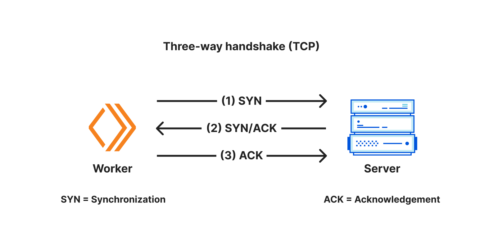
In a modern distributed cloud environment like Workers, where compute is globally distributed (so it’s close to users) and functions are short-lived (so you’re billed no more than is needed), connecting to traditional databases has been both slow and unscalable. Slow because it takes upwards of seven round-trips (TCP handshake; TLS negotiation; then auth) to establish the connection, and unscalable because databases like PostgreSQL have a high resource cost per connection. Even just a couple of hundred connections to a database can consume non-negligible memory, separate from any memory needed for queries.
Our friends over at Neon (a popular serverless Postgres provider) wrote about this, and even released a WebSocket proxy and driver to reduce the connection overhead, but are still fighting uphill in the snow: even with a custom driver, we’re down to 4 round-trips, each still potentially taking 50-200 milliseconds or more. When those connections are long-lived, that’s OK — it might happen once every few hours at best. But when they’re scoped to an individual function invocation, and are only useful for a few milliseconds to minutes at best — your code spends more time waiting. It’s effectively another kind of cold start: having to initiate a fresh connection to your database before making a query means that using a traditional database in a distributed or serverless environment is (to put it lightly) really slow.
To combat this, Hyperdrive does two things.
First, it maintains a set of regional database connection pools across Cloudflare’s network, so a Cloudflare Worker avoids making a fresh connection to a database on every request. Instead, the Worker can establish a connection to Hyperdrive (fast!), with Hyperdrive maintaining a pool of ready-to-go connections back to the database. Since a database can be anywhere from 30ms to (often) 300ms away over a single round-trip (let alone the seven or more you need for a new connection), having a pool of available connections dramatically reduces the latency issue that short-lived connections would otherwise suffer.
Second, it understands the difference between read (non-mutating) and write (mutating) queries and transactions, and can automatically cache your most popular read queries: which represent over 80% of most queries made to databases in typical web applications. That product listing page that tens of thousands of users visit every hour; open jobs on a major careers site; or even queries for config data that changes occasionally; a tremendous amount of what is queried does not change often, and caching it closer to where the user is querying it from can dramatically speed up access to that data for the next ten thousand users. Write queries, which can’t be safely cached, still get to benefit from both Hyperdrive’s connection pooling and Cloudflare’s global network: being able to take the fastest routes across the Internet across our backbone cuts down latency there, too.
Even if your database is on the other side of the country, 70ms x 6 round-trips is a lot of time for a user to be waiting for a query response.
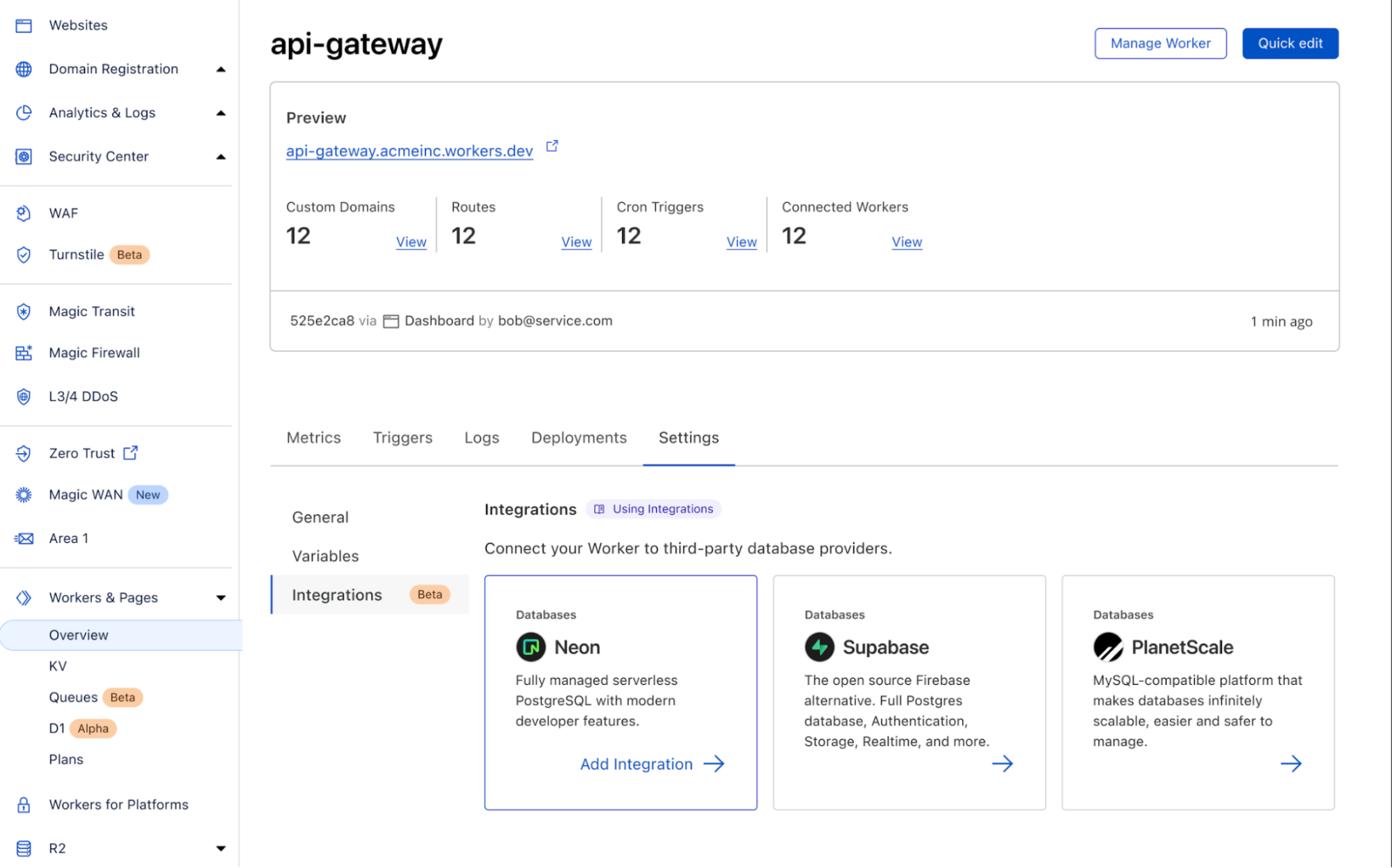
Hyperdrive works not only with PostgreSQL databases — including Neon, Google Cloud SQL, AWS RDS, and Timescale, but also PostgreSQL-compatible databases like Materialize (a powerful stream-processing database), CockroachDB (a major distributed database), Google Cloud’s AlloyDB, and AWS Aurora Postgres.
We’re also working on bringing support for MySQL, including providers like PlanetScale, by the end of the year, with more database engines planned in the future.
The magic connection string
One of the major design goals for Hyperdrive was the need for developers to keep using their existing drivers, query builder and ORM (Object-Relational Mapper) libraries. It wouldn’t have mattered how fast Hyperdrive was if we required you to migrate away from your favorite ORM and/or rewrite hundreds (or more) lines of code & tests to benefit from Hyperdrive’s performance.
The magic behind Hyperdrive is that you can start using it in your existing Workers applications, with your existing queries, just by swapping out your connection string for the one Hyperdrive generates instead.
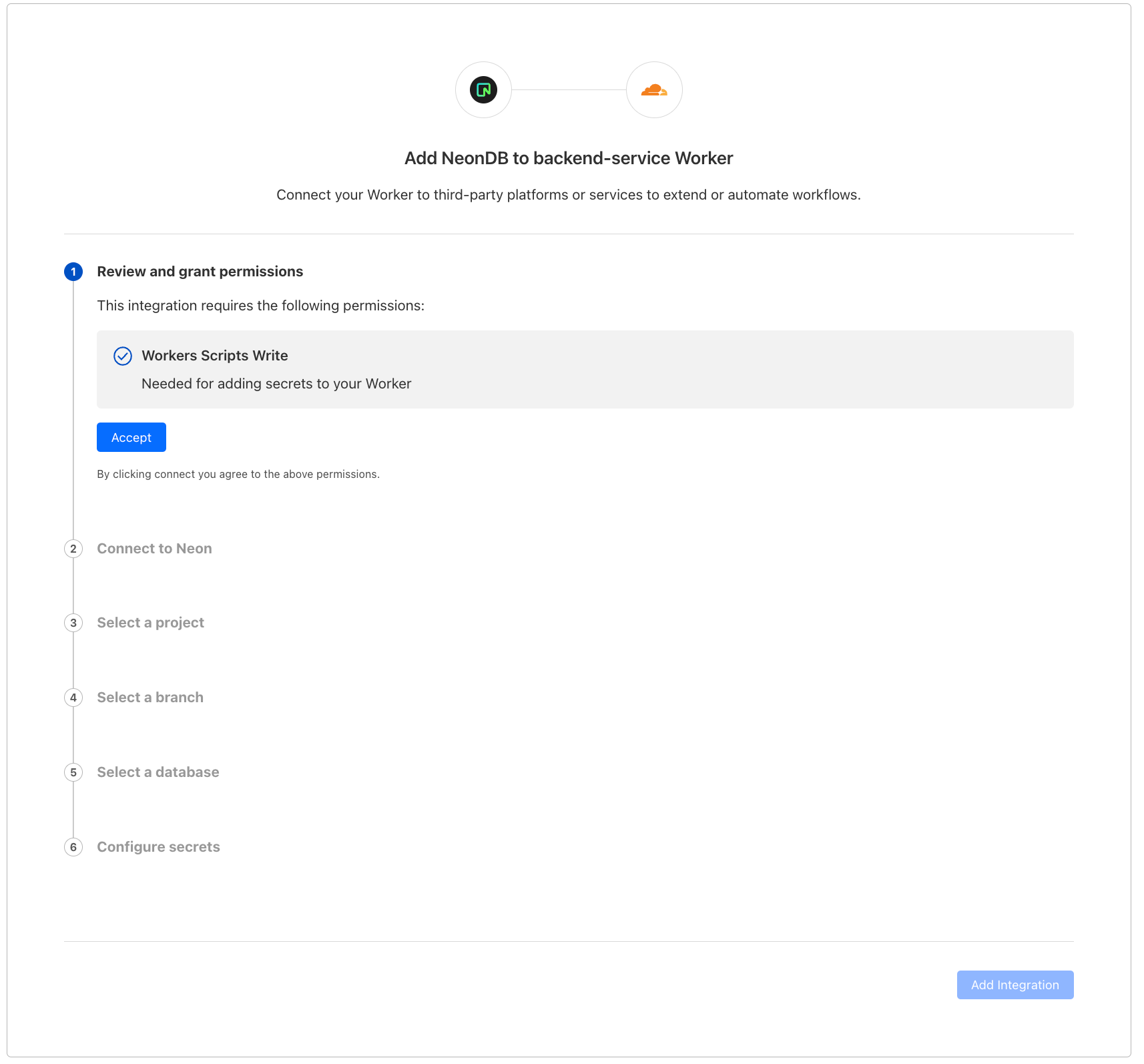
Creating a Hyperdrive
With an existing database ready to go — in this example, we’ll use a Postgres database from Neon — it takes less than a minute to get Hyperdrive running (yes, we timed it).
If you don’t have an existing Cloudflare Workers project, you can quickly create one:
$ npm create cloudflare@latest
# Call the application "hyperdrive-demo"
# Choose "Hello World Worker" as your template
From here, we just need the database connection string for our database and a quick wrangler command-line invocation to have Hyperdrive connect to it.
# Using wrangler v3.8.0 or above
wrangler hyperdrive databases create a-faster-database --connection-string="postgres://user:[email protected]/neondb"

# This will return an ID: we'll use this in the next step
[[hyperdrive]]
name = "HYPERDRIVE"
database_id = "cdb28782-0dfc-4aca-a445-a2c318fb26fd"
We can now write a Worker — or take an existing Worker script — and use Hyperdrive to speed up connections and queries to our existing database. We use node-postgres here, but we could just as easily use Drizzle ORM.
import { Client } from 'pg';

export interface Env {
	HYPERDRIVE: Hyperdrive;
}

export default {
	async fetch(request: Request, env: Env, ctx: ExecutionContext) {
		console.log(JSON.stringify(env));
		// Create a database client that connects to our database via Hyperdrive
		//
		// Hyperdrive generates a unique connection string you can pass to
		// supported drivers, including node-postgres, Postgres.js, and the many
		// ORMs and query builders that use these drivers.
		const client = new Client({ connectionString: env.HYPERDRIVE.connectionString });

		try {
			// Connect to our database
			await client.connect();

			// A very simple test query
			let result = await client.query({ text: 'SELECT * FROM pg_tables' });

			// Return our result rows as JSON
			return Response.json({ result: result });
		} catch (e) {
			console.log(e);
			return Response.json({ error: JSON.stringify(e) }, { status: 500 });
		}
	},
};
The code above is intentionally simple, but hopefully you can see the magic: our database driver gets a connection string from Hyperdrive, and is none-the-wiser. It doesn’t need to know anything about Hyperdrive, we don’t have to toss out our favorite query builder library, and we can immediately realize the speed benefits when making queries.
Connections are automatically pooled and kept warm, our most popular queries are cached, and our entire application gets faster.
We think Hyperdrive is critical to accessing your existing databases when building on Cloudflare Workers: traditional databases were just never designed for a world where clients are globally distributed.
Hyperdrive’s connection pooling will always be free, for both database protocols we support today and new database protocols we add in the future. Just like DDoS protection and our global CDN, we think access to Hyperdrive’s core feature is too useful to hold back.
During the open beta, Hyperdrive itself will not incur any charges for usage, regardless of how you use it. We’ll be announcing more details on how Hyperdrive will be priced closer to GA (early in 2024), with plenty of notice.
Time to query
So where to from here for Hyperdrive?
We’re planning on bringing Hyperdrive to GA in early 2024 — and we’re focused on landing more controls over how we cache & automatically invalidate based on writes, detailed query and performance analytics (soon!), support for more database engines (including MySQL) as well as continuing to work on making it even faster.
We’re also working to enable private network connectivity via Magic WAN and Cloudflare Tunnel, so that you can connect to databases that aren’t (or can’t be) exposed to the public Internet.
To connect Hyperdrive to your existing database, visit our developer docs — it takes less than a minute to create a Hyperdrive and update existing code to use it. Join the #hyperdrive-beta channel in our Developer Discord to ask questions, surface bugs, and talk to our Product & Engineering teams directly.
D1 is now in open beta, and the theme is “scale”: with higher per-database storage limits and the ability to create more databases, we’re unlocking the ability for developers to build production-scale applications on D1. Any developers with an existing paid Workers plan don’t need to lift a finger to benefit: we’ve retroactively applied this to all existing D1 databases.
D1 our native serverless database, which we launched into alpha in November last year: the queryable database complement to Workers KV, Durable Objects and R2.
When we set out to build D1, we knew a few things for certain: it needed to be fast, it needed to be incredibly easy to create a database, and it needed to be SQL-based.
That last one was critical: so that developers could a) avoid learning another custom query language and b) make it easier for existing query buildings, ORM (object relational mapper) libraries and other tools to connect to D1 with minimal effort. From this, we’ve seen a huge number of projects build support in for D1: from support for D1 in the Drizzle ORM and Kysely, to the T4 App, a full-stack toolkit that uses D1 as its database.
We also knew that D1 couldn’t be the only way to query a database from Workers: for teams with existing databases and thousands of lines of SQL or existing ORM code, migrating across to D1 isn’t going to be an afternoon’s work. For those teams, we built Hyperdrive, allowing you to connect to your existing databases and make them feel global. We think this gives teams flexibility: combine D1 and Workers for globally distributed apps, and use Hyperdrive for querying the databases you have in legacy clouds and just can’t get rid of overnight.
Larger databases, and more of them
This has been the biggest ask from the thousands of D1 users throughout the alpha: not just more databases, but also bigger databases.
Developers on the Workers paid plan will now be able to grow each database up to 2GB and create 25 databases (up from 500MB and 10).
We’ll be continuing to work on unlocking even larger databases over the coming weeks and months: developers using the D1 beta will see automatic increases to these limits published on D1’s public changelog.
One of the biggest impediments to double-digit-gigabyte databases is performance: we want to ensure that a database can load in and be ready really quickly — cold starts of seconds (or more) just aren’t acceptable. A 10GB or 20GB database that takes 15 seconds before it can answer a query ends up being pretty frustrating to use.
Users on the Workers free plan will keep the ten 500MB databases (changelog) forever: we want to give more developers the room to experiment with D1 and Workers before jumping in.
Time Travel is here
Time Travel allows you to roll your database back to a specific point in time: specifically, any minute in the last 30 days. And it’s enabled by default for every D1 database, doesn’t cost any more, and doesn’t count against your storage limit.
For those who have been keeping tabs: we originally announced Time Travel earlier this year, and made it available to all D1 users in July. At its core, it’s deceptively simple: Time Travel introduces the concept of a “bookmark” to D1. A bookmark represents the state of a database at a specific point in time, and is effectively an append-only log. Time Travel can take a timestamp and turn it into a bookmark, or a bookmark directly: allowing you to restore back to that point. Even better: restoring doesn’t prevent you from going back further.
We think Time Travel works best with an example, so let’s make a change to a database: one with an Order table that stores every order made against our e-commerce store:
# To illustrate: we have 89,185 unique addresses in our order database.
# To illustrate: we have 89,185 unique addresses in our order database.
➜  wrangler d1 execute northwind --command "SELECT count(distinct ShipAddress) FROM [Order]"
┌──────────┐
│ count(*) │
├──────────┤
│ 89185    │
└──────────┘
OK, great. Now what if we wanted to make a change to a specific set of orders: an address change or freight company change?
# I think we might be forgetting something here...
➜  wrangler d1 execute northwind --command "UPDATE [Order] SET ShipAddress = 'Av. Veracruz 38, Roma Nte., Cuauhtémoc, 06700 Ciudad de México, CDMX, Mexico'
Wait: we’ve made a mistake that many, many folks have before: we forgot the WHERE clause on our UPDATE query. Instead of updating a specific order Id, we’ve instead updated the ShipAddress for every order in our table.
# Every order is now going to a wine bar in Mexico City.
➜  wrangler d1 execute northwind --command "SELECT count(distinct ShipAddress) FROM [Order]"
┌──────────┐
│ count(*) │
├──────────┤
│ 1        │
└──────────┘
Panic sets in. Did we remember to make a backup before we did this? How long ago was it? Did we turn on point-in-time recovery? It seemed potentially expensive at the time…
It’s OK. We’re using D1. We can Time Travel. It’s on by default: let’s fix this and travel back a few minutes.
# Let's go back in time.
➜  wrangler d1 time-travel restore northwind --timestamp="2023-09-23T14:20:00Z"

🚧 Restoring database northwind from bookmark 0000000b-00000002-00004ca7-9f3dba64bda132e1c1706a4b9d44c3c9
✔ OK to proceed (y/N) … yes

⚡️ Time travel in progress...
✅ Database dash-db restored back to bookmark 00000000-00000004-00004ca7-97a8857d35583887de16219c766c0785
↩️ To undo this operation, you can restore to the previous bookmark: 00000013-ffffffff-00004ca7-90b029f26ab5bd88843c55c87b26f497
We think that Time Travel becomes even more powerful when you have many smaller databases, too: the downsides of any restore operation is reduced further and scoped to a single user or tenant.
This is also just the beginning for Time Travel: we’re working to support not just only restoring a database, but also the ability to fork from and overwrite existing databases. If you can fork a database with a single command and/or test migrations and schema changes against real data, you can de-risk a lot of the traditional challenges that working with databases has historically implied.
Row-based pricing
Back in May we announced pricing for D1, to a lot of positive feedback around how much we’d included in our Free and Paid plans. In August, we published a new row-based model, replacing the prior byte-units, that makes it easier to predict and quantify your usage. Specifically, we moved to rows as it’s easier to reason about: if you’re writing a row, it doesn’t matter if it’s 1KB or 1MB. If your read query uses an indexed column to filter on, you’ll see not only performance benefits, but cost savings too.
Here’s D1’s pricing — almost everything has stayed the same, with the added benefit of charging based on rows:
As before, D1 does not charge you for “database hours”, the number of databases, or point-in-time recovery (Time Travel) — just query D1 and pay for your reads, writes, and storage — that’s it.
We believe this makes D1 not only far more cost-efficient, but also makes it easier to manage multiple databases to isolate customer data or prod vs. staging: we don’t care which database you query. Manage your data how you like, separate your customer data, and avoid having to fall for the trap of “Billing Based Architecture”, where you build solely around how you’re charged, even if it’s not intuitive or what makes sense for your team.
To make it easier to both see how much a given query charges and when to optimize your queries with indexes, D1 also returns the number of rows a query read or wrote (or both) so that you can understand how it’s costing you in both cents and speed.
For example, the following query filters over orders based on date:
The unindexed query above scans 16,800 rows. Even if we don’t optimize it, D1 includes 25 billion queries per month for free, meaning we could make this query 1.4 million times for a whole month before having to worry about extra costs.
But we can do better with an index:
CREATE INDEX IF NOT EXISTS idx_orders_date ON [Order](ShippedDate)
With the index created, let’s see how many rows our query needs to read now:
The same query with an index on the ShippedDate column reads just 417 rows: not only it is faster (duration is in milliseconds!), but it costs us less: we could run this query 59 million times per month before we’d have to pay any more than what the $5 Workers plan gives us.
D1 also exposes row counts via both the Cloudflare dashboard and our GraphQL analytics API: so not only can you look at this per-query when you’re tuning performance, but also break down query patterns across all of your databases.
D1 for Platforms
Throughout D1’s alpha period, we’ve both heard from and worked with teams who are excited about D1’s ability to scale out horizontally: the ability to deploy a database-per-customer (or user!) in order to keep data closer to where teams access it and more strongly isolate that data from their other users.
Teams building the next big thing on Workers for Platforms — think of it as “Functions as a Service, as a Service” — can use D1 to deploy a database per user — keeping customer data strongly separated from each other.
For example, and as one of the early adopters of D1, RONIN is building an edge-first content & data platform backed by a dedicated D1 database per customer, which allows customers to place data closer to users and provides each customer isolation from the queries of others.
Instead of spinning up and managing countless traditional database instances, RONIN uses D1 for Platforms to offer automatic infinite scalability at the edge. This allows RONIN to focus on providing a sleek, intuitive editing experience for your content & data.
When it comes to enabling “D1 for Platforms”, we’ve thought about this in a few ways from the very beginning:
Support for more than 100,000+ databases for Workers for Platforms users (there’s no limit, but if we said “unlimited” you might not believe us).
D1’s pricing – you don’t pay per-database or for “idle databases”. If you have a range of users, from thousands of QPS down to 1-2 every 10 minutes — you aren’t paying more for “database hours” on the less trafficked databases, or having to plan around spiky workloads across your user-base.
The ability to programmatically configure more databases via D1’s HTTP APIand attach them to your Worker without re-deploying. There’s no “provisioning” delay, either: you create the database, and it’s immediately ready to query by you or your users.
Detailed per-database analytics, so you can understand which databases are being used and how they’re being queried via D1’s GraphQL analytics API.
If you’re building the next big platform on top of Workers & want to use D1 at scale — whether you’re part of the Workers Launchpad program or not — reach out.
What’s next for D1?
We’re setting a clear goal: we want to make D1 “generally available” (GA) for production use-cases by early next year(Q1 2024). Although you can already use D1 without a waitlist or approval process, we understand that the GA label is an important one for many when it comes to a database (and as do we).
Between now and GA, we’re working on some really key parts of the D1 vision, with a continued focus on reliability and performance.
One of the biggest remaining pieces of that vision is global read replication, which we wrote about earlier this year. Importantly, replication will be free, won’t multiply your storage consumption, and will still enable session consistency (read-your-writes). Part of D1’s mission is about getting data closer to where users are, and we’re excited to land it.
We’re also working to expand Time Travel, D1’s built-in point-in-time recovery capabilities, so that you can branch and/or clone a database from a specific point-in-time on the fly.
We’ll also be progressively opening up our limits around per-database storage, unlocking more storage per account, and the number of databases you can create over the rest of this year, so keep an eye on the D1 changelog (or your inbox).
In the meantime, if you haven’t yet used D1, you can get started right now, visit D1’s developer documentation to spark some ideas, or join the #d1-beta channel on our Developer Discord to talk to other D1 developers and our product-engineering team.
SQL databases in Amazon Web Services (AWS), using services like Amazon Relational Database Service (Amazon RDS) and Amazon Aurora, offer software architects scalability, automated management, robust security, and cost-efficiency. This combination simplifies database management, improves performance, enhances security, and allows architects to create efficient and scalable software systems.
In this post, we introduce caching strategies and continue with real case studies that use services like Amazon ElastiCache or Amazon MemoryDB in real workloads where customers share the reasoning behind their approaches. It’s very important to understand the context for leveraging a specific solution or pattern, and these resources answer many commonly asked questions.
For software architects and developers, striking the right balance between operational complexity and cost efficiency is a perpetual challenge. Often, provisioning a separate database for each workload is the gold standard, offering unmatched isolation and granular operational controls. However, it’s not always the most cost-effective or operationally manageable approach. Through a real-world success story, we explore how Aurora played a pivotal role in helping VMware Aria Cost, powered by CloudHealth, consolidate a staggering 166 self-managed MySQL databases onto 62 Aurora clusters.
Amazon RDS Blue/Green Deployments revolutionizes the way you handle database updates, ensuring safety and simplicity, often achieving rapid updates in just a minute, with zero data loss. Meanwhile, Amazon RDS Optimized Writes turbocharges write transaction throughput by as much as double, without any additional extra cost. Amazon RDS Optimized Reads steps in to deliver a significant boost to database performance, processing queries up to 50% faster.
Discover how to leverage these capabilities of Amazon RDS in this one-hour video from re:Invent 2022.
In the world of mission-critical workloads, the importance of a robust disaster recovery (DR) strategy cannot be overstated. It’s the lifeline that ensures databases stay operational, even in the face of unexpected events. Discover the intricacies of crafting a dependable, cross-Region DR strategy tailored to Amazon RDS for SQL Server.
In this AWS Developers session, we uncover the best practices for efficiently managing and monitoring these cross-Region read replicas. From proactive monitoring to fine-tuning, you’ll gain the insights needed to keep your DR strategy finely tuned.
Aurora represents a paradigm shift in relational databases, boasting an architecture that decouples computational processes from data storage. It introduces advanced features, such as Global Database and low-latency read replicas, redefining the landscape of database management.
This modern database service excels in performance, scalability, and high availability on a large scale, offering compatibility with both MySQL and PostgreSQL open-source editions. Additionally, it provides an array of developer tools tailored for serverless and machine learning-driven applications.
This re:Invent 2022 session is an in-depth exploration of some of Aurora’s most compelling features, including Aurora Serverless v2 and Global Database. We also share the most recent innovations aimed at enhancing performance, scalability, and security while streamlining operational processes.
If you're anywhere near the developer community, it's almost impossible to avoid the impact that AI’s recent advancements have had on the ecosystem. Whether you're using AI in your workflow to improve productivity, or you’re shipping AI based features to your users, it’s everywhere. The focus on AI improvements are extraordinary, and we’re super excited about the opportunities that lay ahead, but it's not enough.
Not too long ago, if you wanted to leverage the power of AI, you needed to know the ins and outs of machine learning, and be able to manage the infrastructure to power it.
As a developer platform with over one million active developers, we believe there is so much potential yet to be unlocked, so we’re changing the way AI is delivered to developers. Many of the current solutions, while powerful, are based on closed, proprietary models and don't address privacy needs that developers and users demand. Alternatively, the open source scene is exploding with powerful models, but they’re simply not accessible enough to every developer. Imagine being able to run a model, from your code, wherever it’s hosted, and never needing to find GPUs or deal with setting up the infrastructure to support it.
That's why we are excited to launch Workers AI – an AI inference as a service platform, empowering developers to run AI models with just a few lines of code, all powered by our global network of GPUs. It's open and accessible, serverless, privacy-focused, runs near your users, pay-as-you-go, and it's built from the ground up for a best in class developer experience.
Workers AI – making inference just work
We’re launching Workers AI to put AI inference in the hands of every developer, and to actually deliver on that goal, it should just work out of the box. How do we achieve that?
At the core of everything, it runs on the right infrastructure – our world-class network of GPUs
We provide off-the-shelf models that run seamlessly on our infrastructure
Finally, deliver it to the end developer, in a way that’s delightful. A developer should be able to build their first Workers AI app in minutes, and say “Wow, that’s kinda magical!”.
So what exactly is Workers AI? It’s another building block that we’re adding to our developer platform – one that helps developers run well-known AI models on serverless GPUs, all on Cloudflare’s trusted global network. As one of the latest additions to our developer platform, it works seamlessly with Workers + Pages, but to make it truly accessible, we’ve made it platform-agnostic, so it also works everywhere else, made available via a REST API.
Models you know and love
We’re launching with a curated set of popular, open source models, that cover a wide range of inference tasks:
Text generation (large language model): meta/llama-2-7b-chat-int8
Text classification: huggingface/distilbert-sst-2-int8
Image classification: microsoft/resnet-50
Embeddings: baai/bge-base-en-v1.5
You can browse all available models in your Cloudflare dashboard, and soon you’ll be able to dive into logs and analytics on a per model basis!
This is just the start, and we’ve got big plans. After launch, we’ll continue to expand based on community feedback. Even more exciting – in an effort to take our catalog from zero to sixty, we’re announcing a partnership with Hugging Face, a leading AI community + hub. The partnership is multifaceted, and you can read more about it here, but soon you’ll be able to browse and run a subset of the Hugging Face catalog directly in Workers AI.
Accessible to everyone
Part of the mission of our developer platform is to provide all the building blocks that developers need to build the applications of their dreams. Having access to the right blocks is just one part of it — as a developer your job is to put them together into an application. Our goal is to make that as easy as possible.
To make sure you could use Workers AI easily regardless of entry point, we wanted to provide access via: Workers or Pages to make it easy to use within the Cloudflare ecosystem, and via REST API if you want to use Workers AI with your current stack.
Here’s a quick CURL example that translates some text from English to French:
curl https://api.cloudflare.com/client/v4/accounts/{ACCOUNT_ID}/ai/run/@cf/meta/@cf/meta/m2m100-1.2b \
-H "Authorization: Bearer {API_TOKEN}" \
	-d '{ "text": "I'll have an order of the moule frites", "target_lang": "french" }'
Use it with any stack, anywhere – your favorite Jamstack framework, Python + Django/Flask, Node.js, Ruby on Rails, the possibilities are endless. And deploy
Designed for developers
Developer experience is really important to us. In fact, most of this post has been about just that. Making sure it works out of the box. Providing popular models that just work. Being accessible to all developers whether you build and deploy with Cloudflare or elsewhere. But it’s more than that – the experience should be frictionless, zero to production should be fast, and it should feel good along the way.
Let’s walk through another example to show just how easy it is to use! We’ll run Llama 2, a popular large language model open sourced by Meta, in a worker.
We’ll assume you have some of the basics already complete (Cloudflare account, Node, NPM, etc.), but if you don’t this guide will get you properly set up!
1. Create a Workers project
Create a new project named workers-ai by running:
$ npm create cloudflare@latest
When setting up your workers-ai worker, answer the setup questions as follows:
Enter workers-ai for the app name
Choose Hello World script for the type of application
Select yes to using TypeScript
Select yes to using Git
Select no to deploying
Lastly navigate to your new app directory:
cd workers-ai
2. Connect Workers AI to your worker
Create a Workers AI binding, which allows your worker to access the Workers AI service without having to manage an API key yourself.
To bind Workers AI to your worker, add the following to the end of your wrangler.toml file:
[ai]
binding = "AI" #available in your worker via env.AI
You can also bind Workers AI to a Pages Function. For more information, refer to Functions Bindings.
3. Install the Workers AI client library
npm install @cloudflare/ai --save-dev
4. Run an inference task in your worker
Update the source/index.ts with the following code:
import { Ai } from '@cloudflare/ai'
export default {
  async fetch(request, env) {
    const ai = new Ai(env.AI);
    const input = { prompt: "What's the origin of the phrase 'Hello, World'" };
    const output = await ai.run('@cf/meta/llama-2-7b-chat-int8', input );
    return new Response(JSON.stringify(output));
  },
};
5. Develop locally with Wrangler
While in your project directory, test Workers AI locally by running:
$ npx wranlger dev --remote
Note – These models currently only run on Cloudflare’s network of GPUs (and not locally), so setting `–remote` above is a must, and you’ll be prompted to log in at this point.
Wrangler will give you a URL (most likely localhost:8787). Visit that URL, and you’ll see a response like this
{
  "response": "Hello, World is a common phrase used to test the output of a computer program, particularly in the early stages of programming. The phrase "Hello, World!" is often the first program that a beginner learns to write, and it is included in many programming language tutorials and textbooks as a way to introduce basic programming concepts. The origin of the phrase "Hello, World!" as a programming test is unclear, but it is believed to have originated in the 1970s. One of the earliest known references to the phrase is in a 1976 book called "The C Programming Language" by Brian Kernighan and Dennis Ritchie, which is considered one of the most influential books on the development of the C programming language.
}
6. Deploy your worker
Finally, deploy your worker to make your project accessible on the Internet:
$ npx wranlger dev --remote
# Outputs: https://workers-ai.<YOUR_SUBDOMAIN>.workers.dev
And that’s it. You can literally go from zero to deployed AI in minutes. This is obviously a simple example, but shows how easy it is to run Workers AI from any project.
Privacy by default
When Cloudflare was founded, our value proposition had three pillars: more secure, more reliable, and more performant. Over time, we’ve realized that a better Internet is also a more private Internet, and we want to play a role in building it.
That’s why Workers AI is private by default – we don’t train our models, LLM or otherwise, on your data or conversations, and our models don’t learn from your usage. You can feel confident using Workers AI in both personal and business settings, without having to worry about leaking your data. Other providers only offer this fundamental feature with their enterprise version. With us, it’s built in for everyone.
We’re also excited to support data localization in the future. To make this happen, we have an ambitious GPU rollout plan – we’re launching with seven sites today, roughly 100 by the end of 2023, and nearly everywhere by the end of 2024. Ultimately, this will empower developers to keep delivering killer AI features to their users, while staying compliant with their end users’ data localization requirements.
The power of the platform
Vector database – Vectorize
Workers AI is all about running Inference, and making it really easy to do so, but sometimes inference is only part of the equation. Large language models are trained on a fixed set of data, based on a snapshot at a specific point in the past, and have no context on your business or use case. When you submit a prompt, information specific to you can increase the quality of results, making it more useful and relevant. That’s why we’re also launching Vectorize, our vector database that’s designed to work seamlessly with Workers AI. Here’s a quick overview of how you might use Workers AI + Vectorize together.
Example: Use your data (knowledge base) to provide additional context to an LLM when a user is chatting with it.
Generate initial embeddings: run your data through Workers AI using an embedding model. The output will be embeddings, which are numerical representations of those words.
Insert those embeddings into Vectorize: this essentially seeds the vector database with your data, so we can later use it to retrieve embeddings that are similar to your users’ query
Generate embedding from user question: when a user submits a question to your AI app, first, take that question, and run it through Workers AI using an embedding model.
Get context from Vectorize: use that embedding to query Vectorize. This should output embeddings that are similar to your user’s question.
Create context aware prompt:Now take the original text associated with those embeddings, and create a new prompt combining the text from the vector search, along with the original question
Run prompt: run this prompt through Workers AI using an LLM model to get your final result
AI Gateway
That covers a more advanced use case. On the flip side, if you are running models elsewhere, but want to get more out of the experience, you can run those APIs through our AI gateway to get features like caching, rate-limiting, analytics and logging. These features can be used to protect your end point, monitor and optimize costs, and also help with data loss prevention. Learn more about AI gateway here.
Start building today
Try it out for yourself, and let us know what you think. Today we’re launching Workers AI as an open Beta for all Workers plans – free or paid. That said, it’s super early, so…
Warning – It’s an early beta
Usage is not currently recommended for production apps, and limits + access are subject to change.
Limits
We’re initially launching with limits on a per-model basis
@cf/meta/llama-2-7b-chat-int8: 5 reqs/min
All other modes are between 120-180 reqs/min
Checkout our docs for a full overview of our limits.
Pricing
What we released today is just a small preview to give you a taste of what’s coming (we simply couldn’t hold back), but we’re looking forward to putting the full-throttle version of Workers AI in your hands.
We realize that as you approach building something, you want to understand: how much is this going to cost me? Especially with AI costs being so easy to get out of hand. So we wanted to share the upcoming pricing of Workers AI with you.
While we won’t be billing on day one, we are announcing what we expect our pricing will look like.
Users will be able to choose from two ways to run Workers AI:
Fast Twitch Neurons (FTN) – running at nearest user location at $1.25 / 1k neurons
You may be wondering — what’s a neuron?
Neurons are a way to measure AI output that always scales down to zero (if you get no usage, you will be charged for 0 neurons). To give you a sense of what you can accomplish with a thousand neurons, you can: generate 130 LLM responses, 830 image classifications, or 1,250 embeddings.
Our goal is to help our customers pay only for what they use, and choose the pricing that best matches their use case, whether it’s price or latency that is top of mind.
What’s on the roadmap?
Workers AI is just getting started, and we want your feedback to help us make it great. That said, there are some exciting things on the roadmap.
More models, please
We're launching with a solid set of models that just work, but will continue to roll out new models based on your feedback. If there’s a particular model you'd love to see on Workers AI, pop into our Discord and let us know!
In addition to that, we're also announcing a partnership with Hugging Face, and soon you'll be able to access and run a subset of the Hugging Face catalog directly from Workers AI.
Analytics + observability
Up to this point, we’ve been hyper focussed on one thing – making it really easy for any developer to run powerful AI models in just a few lines of code. But that’s only one part of the story. Up next, we’ll be working on some analytics and observability capabilities to give you insights into your usage + performance + spend on a per-model basis, plus the ability to fig into your logs if you want to do some exploring.
A road to global GPU coverage
Our goal is to be the best place to run inference on Region: Earth, so we're adding GPUs to our data centers as fast as we can.
We plan to be in 100 data centers by the end this year
And nearly everywhere by the end of 2024
We’re really excited to see you build – head over to our docs to get started.
If you need inspiration, want to share something you’re building, or have a question – pop into our Developer Discord.
Vectorize is our brand-new vector database offering, designed to let you build full-stack, AI-powered applications entirely on Cloudflare’s global network: and you can start building with it right away. Vectorize is in open beta, and is available to any developer using Cloudflare Workers.
You can use Vectorize with Workers AI to power semantic search, classification, recommendation and anomaly detection use-cases directly with Workers, improve the accuracy and context of answers from LLMs (Large Language Models), and/or bring-your-own embeddings from popular platforms, including OpenAI and Cohere.
Visit Vectorize’s developer documentation to get started, or read on if you want to better understand what vector databases do and how Vectorize is different.
Why do I need a vector database?
Machine learning models can’t remember anything: only what they were trained on.
Vector databases are designed to solve this, by capturing how an ML model represents data — including structured and unstructured text, images and audio — and storing it in a way that allows you to compare against future inputs. This allows us to leverage the power of existing machine-learning models and LLMs (Large Language Models) for content they haven’t been trained on: which, given the tremendous cost of training models, turns out to be extremely powerful.
To better illustrate why a vector database like Vectorize is useful, let’s pretend they don’t exist, and see how painful it is to give context to an ML model or LLM for a semantic search or recommendation task. Our goal is to understand what content is similar to our query and return it: based on our own dataset.
Our user query comes in: they’re searching for “how to write to R2 from Cloudflare Workers”
We load up our entire documentation dataset — a thankfully “small” dataset at about 65,000 sentences, or 2.1 GB — and provide it alongside the query from our user. This allows the model to have the context it needs, based on our data.
We wait.
(A long time)
We get our similarity scores back, with the sentences most similar to the user’s query, and then work to map those back to URLs before we return our search results.
… and then another query comes in, and we have to start this all over again.
In practice, this isn’t really possible: we can’t pass that much context in an API call (prompt) to most machine learning models, and even if we could, it’d take tremendous amounts of memory and time to process our dataset over-and-over again.
With a vector database, we don’t have to repeat step 2: we perform it once, or as our dataset updates, and use our vector database to provide a form of long-term memory for our machine learning model. Our workflow looks a little more like this:
We load up our entire documentation dataset, run it through our model, and store the resulting vector embeddings in our vector database (just once).
For each user query (and only the query) we ask the same model and retrieve a vector representation.
We query our vector database with that query vector, which returns the vectors closest to our query vector.
If we looked at these two flows side by side, we can quickly see how inefficient and impractical it is to use our own dataset with an existing model without a vector database:
Using a vector database to help machine learning models remember.
From this simple example, it’s probably starting to make some sense: but you might also be wondering why you need a vector database instead of just a regular database.
Vectors are the model’s representation of an input: how it maps that input to its internal structure, or “features”. Broadly, the more similar vectors are, the more similar the model believes those inputs to be based on how it extracts features from an input.
This is seemingly easy when we look at example vectors of only a handful of dimensions. But with real-world outputs, searching across 10,000 to 250,000 vectors, each potentially 1,536 dimensions wide, is non-trivial. This is where vector databases come in: to make search work at scale, vector databases use a specific class of algorithm, such as k-nearest neighbors (kNN) or other approximate nearest neighbor (ANN) algorithms to determine vector similarity.
And although vector databases are extremely useful when building AI and machine learning powered applications, they’re not only useful in those use-cases: they can be used for a multitude of classification and anomaly detection tasks. Knowing whether a query input is similar — or potentially dissimilar — from other inputs can power content moderation (does this match known-bad content?) and security alerting (have I seen this before?) tasks as well.
Building a recommendation engine with vector search
We built Vectorize to be a powerful partner to Workers AI: enabling you to run vector search tasks as close to users as possible, and without having to think about how to scale it for production.
We’re going to take a real world example — building a (product) recommendation engine for an e-commerce store — and simplify a few things.
Our goal is to show a list of “relevant products” on each product listing page: a perfect use-case for vector search. Our input vectors in the example are placeholders, but in a real world application we would generate them based on product descriptions and/or cart data by passing them through a sentence similarity model (such as Worker’s AI’s text embedding model)
Each vector represents a product across our store, and we associate the URL of the product with it. We could also set the ID of each vector to the product ID: both approaches are valid. Our query — vector search — represents the product description and content for the product user is currently viewing.
Let’s step through what this looks like in code: this example is pulled straight from our developer documentation:
export interface Env {
	// This makes our vector index methods available on env.MY_VECTOR_INDEX.*
	// e.g. env.MY_VECTOR_INDEX.insert() or .query()
	TUTORIAL_INDEX: VectorizeIndex;
}

// Sample vectors: 3 dimensions wide.
//
// Vectors from a machine-learning model are typically ~100 to 1536 dimensions
// wide (or wider still).
const sampleVectors: Array<VectorizeVector> = [
	{ id: '1', values: [32.4, 74.1, 3.2], metadata: { url: '/products/sku/13913913' } },
	{ id: '2', values: [15.1, 19.2, 15.8], metadata: { url: '/products/sku/10148191' } },
	{ id: '3', values: [0.16, 1.2, 3.8], metadata: { url: '/products/sku/97913813' } },
	{ id: '4', values: [75.1, 67.1, 29.9], metadata: { url: '/products/sku/418313' } },
	{ id: '5', values: [58.8, 6.7, 3.4], metadata: { url: '/products/sku/55519183' } },
];

export default {
	async fetch(request: Request, env: Env, ctx: ExecutionContext): Promise<Response> {
		if (new URL(request.url).pathname !== '/') {
			return new Response('', { status: 404 });
		}
		// Insert some sample vectors into our index
		// In a real application, these vectors would be the output of a machine learning (ML) model,
		// such as Workers AI, OpenAI, or Cohere.
		let inserted = await env.TUTORIAL_INDEX.insert(sampleVectors);

		// Log the number of IDs we successfully inserted
		console.info(`inserted ${inserted.count} vectors into the index`);

		// In a real application, we would take a user query - e.g. "durable
		// objects" - and transform it into a vector emebedding first.
		//
		// In our example, we're going to construct a simple vector that should
		// match vector id #5
		let queryVector: Array<number> = [54.8, 5.5, 3.1];

		// Query our index and return the three (topK = 3) most similar vector
		// IDs with their similarity score.
		//
		// By default, vector values are not returned, as in many cases the
		// vectorId and scores are sufficient to map the vector back to the
		// original content it represents.
		let matches = await env.TUTORIAL_INDEX.query(queryVector, { topK: 3, returnVectors: true });

		// We map over our results to find the most similar vector result.
		//
		// Since our index uses the 'cosine' distance metric, scores will range
		// from 1 to -1.  A value of '1' means the vector is the same; the
		// closer to 1, the more similar. Values of -1 (least similar) and 0 (no
		// match).
		// let closestScore = 0;
		// let mostSimilarId = '';
		// matches.matches.map((match) => {
		// 	if (match.score > closestScore) {
		// 		closestScore = match.score;
		// 		mostSimilarId = match.vectorId;
		// 	}
		// });

		return Response.json({
			// This will return the closest vectors: we'll see that the vector
			// with id = 5 has the highest score (closest to 1.0) as the
			// distance between it and our query vector is the smallest.
			// Return the full set of matches so we can see the possible scores.
			matches: matches,
		});
	},
};
The code above is intentionally simple, but illustrates vector search at its core: we insert vectors into our database, and query it for vectors with the smallest distance to our query vector.
Here are the results, with the values included, so we visually observe that our query vector [54.8, 5.5, 3.1] is similar to our highest scoring match: [58.799, 6.699, 3.400] returned from our search. This index uses cosine similarity to calculate the distance between vectors, which means that the closer the score to 1, the more similar a match is to our query vector.
In a real application, we could now quickly return product recommendation URLs based on the most similar products, sorting them by their score (highest to lowest), and increasing the topK value if we want to show more. The metadata stored alongside each vector could also embed a path to an R2 object, a UUID for a row in a D1 database, or a key-value pair from Workers KV.
Workers AI + Vectorize: full stack vector search on Cloudflare
In a real application, we need a machine learning model that can both generate vector embeddings from our original dataset (to seed our database) and quickly turn user queries into vector embeddings too. These need to be from the same model, as each model represents features differently.
Here’s a compact example building an entire end-to-end vector search pipeline on Cloudflare:
import { Ai } from '@cloudflare/ai';
export interface Env {
	TEXT_EMBEDDINGS: VectorizeIndex;
	AI: any;
}
interface EmbeddingResponse {
	shape: number[];
	data: number[][];
}

export default {
	async fetch(request: Request, env: Env, ctx: ExecutionContext): Promise<Response> {
		const ai = new Ai(env.AI);
		let path = new URL(request.url).pathname;
		if (path.startsWith('/favicon')) {
			return new Response('', { status: 404 });
		}

		// We only need to generate vector embeddings just the once (or as our
		// data changes), not on every request
		if (path === '/insert') {
			// In a real-world application, we could read in content from R2 or
			// a SQL database (like D1) and pass it to Workers AI
			const stories = ['This is a story about an orange cloud', 'This is a story about a llama', 'This is a story about a hugging emoji'];
			const modelResp: EmbeddingResponse = await ai.run('@cf/baai/bge-base-en-v1.5', {
				text: stories,
			});

			// We need to convert the vector embeddings into a format Vectorize can accept.
			// Each vector needs an id, a value (the vector) and optional metadata.
			// In a real app, our ID would typicaly be bound to the ID of the source
			// document.
			let vectors: VectorizeVector[] = [];
			let id = 1;
			modelResp.data.forEach((vector) => {
				vectors.push({ id: `${id}`, values: vector });
				id++;
			});

			await env.TEXT_EMBEDDINGS.upsert(vectors);
		}

		// Our query: we expect this to match vector id: 1 in this simple example
		let userQuery = 'orange cloud';
		const queryVector: EmbeddingResponse = await ai.run('@cf/baai/bge-base-en-v1.5', {
			text: [userQuery],
		});

		let matches = await env.TEXT_EMBEDDINGS.query(queryVector.data[0], { topK: 1 });
		return Response.json({
			// We expect vector id: 1 to be our top match with a score of
			// ~0.896888444
			// We are using a cosine distance metric, where the closer to one,
			// the more similar.
			matches: matches,
		});
	},
};
The code above does four things:
It passes the three sentences to Workers AI’s text embedding model (@cf/baai/bge-base-en-v1.5) and retrieves their vector embeddings.
It inserts those vectors into our Vectorize index.
Takes the user query and transforms it into a vector embedding via the same Workers AI model.
Queries our Vectorize index for matches.
This example might look “too” simple, but in a production application, we’d only have to change two things: just insert our vectors once (or periodically via Cron Triggers), and replace our three example sentences with real data stored in R2, a D1 database, or another storage provider.
In fact, this is incredibly similar to how we run Cursor, the AI assistant that can answer questions about Cloudflare Worker: we migrated Cursor to run on Workers AI and Vectorize. We generate text embeddings from our developer documentation using its built-in text embedding model, insert them into a Vectorize index, and transform user queries on the fly via that same model.
BYO embeddings from your favorite AI API
Vectorize isn’t just limited to Workers AI, though: it’s a fully-fledged, standalone vector database.
If you’re already using OpenAI’s Embedding API, Cohere’s multilingual model, or any other embedding API, then you can easily bring-your-own (BYO) vectors to Vectorize.
It works just the same: generate your embeddings, insert them into Vectorize, and pass your queries through the model before you query your index. Vectorize includes a few shortcuts for some of the most popular embedding models.
# Vectorize has ready-to-go presets that set the dimensions and distance metric for popular embeddings models
$ wrangler vectorize create openai-index-example --preset=openai-text-embedding-ada-002
This can be particularly useful if you already have an existing workflow around an existing embeddings API, and/or have validated a specific multimodal or multilingual embeddings model for your use-case.
Making the cost of AI predictable
There’s a tremendous amount of excitement around AI and ML, but there’s also one big concern: that it’s too expensive to experiment with, and hard to predict at scale.
With Vectorize, we wanted to bring a simpler pricing model to vector databases. Have an idea for a proof-of-concept at work? That should fit into our free-tier limits. Scaling up and optimizing your embedding dimensions for performance vs. accuracy? It shouldn’t break the bank.
Importantly, Vectorize aims to be predictable: you don’t need to estimate CPU and memory consumption, which can be hard when you’re just starting out, and made even harder when trying to plan for your peak vs. off-peak hours in production for a brand new use-case. Instead, you’re charged based on the total number of vector dimensions you store, and the number of queries against them each month. It’s our job to take care of scaling up to meet your query patterns.
Here’s the pricing for Vectorize — and if you have a Workers paid plan now, Vectorize is entirely free to use until 2024:
Workers Free (coming soon)
Workers Paid ($5/month)
Queried vector dimensions included
30M total queried dimensions / month
50M total queried dimensions / month
Stored vector dimensions included
5M stored dimensions / month
10M stored dimensions / month
Additional cost
$0.04 / 1M vector dimensions queried or stored
$0.04 / 1M vector dimensions queried or stored
Pricing is based entirely on what you store and query: (total vector dimensions queried + stored) * dimensions_per_vector * price. Query more? Easy to predict. Optimizing for smaller dimensions per vector to improve speed and reduce overall latency? Cost goes down. Have a few indexes for prototyping or experimenting with new use-cases? We don’t charge per-index.
Create as many as you need indexes to prototype new ideas and/or separate production from dev.
As an example: if you load 10,000 Workers AI vectors (384 dimensions each) and make 5,000 queries against your index each day, it’d result in 49 million total vector dimensions queried and still fit into what we include in the Workers Paid plan ($5/month). Better still: we don’t delete your indexes due to inactivity.
Note that while this pricing isn’t final, we expect few changes going forward. We want to avoid the element of surprise: there’s nothing worse than starting to build on a platform and realizing the pricing is untenable after you’ve invested the time writing code, tests and learning the nuances of a technology.
This is also just the beginning of the vector database story for us at Cloudflare. Over the next few weeks and months, we intend to land a new query engine that should further improve query performance, support even larger indexes, introduce sub-index filtering capabilities, increased metadata limits, and per-index analytics.
If you’re looking for inspiration on what to build, see the semantic search tutorial that combines Workers AI and Vectorize for document search, running entirely on Cloudflare. Or an example of how to combine OpenAI and Vectorize to give an LLM more context and dramatically improve the accuracy of its answers.
And if you have questions about how to use Vectorize for our product & engineering teams, or just want to bounce an idea off of other developers building on Workers AI, join the #vectorize and #workers-ai channels on our Developer Discord.
In-memory databases play a critical role in modern computing, particularly in reducing the strain on existing resources, scaling workloads efficiently, and minimizing the cost of infrastructure. The advanced performance capabilities of in-memory databases make them vital for demanding applications characterized by voluminous data, real-time analytics, and rapid response requirements.
In this edition of Let’s Architect!, we are introducing caching strategies and, further, examining case studies that use Amazon Web Services (AWS), like Amazon ElastiCache or Amazon MemoryDB for Redis, in real workloads where customers share the reasoning behind their approaches. It is very important understanding the context for leveraging a specific solution or pattern, and many common questions can be answered with these resources.
Many services built at Amazon rely on caching systems in the background to speed up performance, deal with low latency requirements, and avoid overloading on source databases and other microservices. Operating caches and adding caches into our systems may present complex challenges in terms of monitoring, data consistency, and load on the other components of the system. Indeed, a cache can give big benefits, but it’s also a new component to run and keep healthy. Furthermore, engineers may need to use empirical methods to choose the cache size, expiration policy, and eviction policy: we always have to perform tests and use the metrics to tune the setup.
With this Amazon Builder’s Library resource, you can learn strategies for using caching in your architecture and best practices directly from Amazon’s engineers.
Discover how Yahoo effectively leverages the power of Amazon ElastiCache and data tiering to process an astounding 1.3 million advertising data events per second, all while generating savings of up to 50% on their overall bill.
Data tiering is an ingenious method to scale up to hundreds of terabytes of capacity by intelligently managing data. It achieves this by automatically shifting the least-recently accessed data between RAM and high-performance SSDs.
In this video, you will gain insights into how data tiering operates and how you can unlock ultra-fast speeds and seamless scalability for your workloads in a cost-efficient manner. Furthermore, you can also learn how it’s implemented under the hood.
MemoryDB is a robust, durable database marked by microsecond reads, low single-digit millisecond writes, scalability, and fortified enterprise security. It guarantees an impressive 99.99% availability, coupled with instantaneous recovery without any data loss.
In this session, we explore multiple use cases across sectors, such as Financial Services, Retail, and Media & Entertainment, like payment processing, message brokering, and durable session store applications. Moreover, through a practical demonstration, you can learn how to utilize MemoryDB to establish a microservices message broker for a Media & Entertainment application.
MemoryDB offers the kind of ultra-fast performance that only an in-memory database can deliver, curtailing latency to microseconds and processing 160+ million requests per second —without data loss. In this re:Invent 2022 session, you will understand why Samsung SmartThings selected MemoryDB as the engine to power the next generation of their IoT device connectivity platform, one that processes millions of events every day.
You can also discover the intricate design of MemoryDB and how it ensures data durability without compromising the performance of in-memory operations, thanks to the utilization of a multi-AZ transactional log. This session is an enlightening deep-dive into durable, in-memory data operations.
In this edition of AWS Online Tech Talks, explore Amazon ElastiCache, a managed service that facilitates the seamless setup, operation, and scaling of widely used, open-source–compatible, in-memory datastores in the cloud environment. This service positions you to develop data-intensive applications or enhance the performance of your existing databases through high-throughput, low-latency, in-memory datastores. Learn how it is leveraged for caching, session stores, gaming, geospatial services, real-time analytics, and queuing functionalities.
This course can help cultivate a deeper understanding of Amazon ElastiCache, and how it can be used to accelerate your data processing while maintaining robustness and reliability.
During Developer Week we announced Database Integrations on Workers a new and seamless way to connect with some of the most popular databases. You select the provider, authorize through an OAuth2 flow and automatically get the right configuration stored as encrypted environment variables to your Worker.
Today we are thrilled to announce that we have been working with Upstash to expand our integrations catalog. We are now offering three new integrations: Upstash Redis, Upstash Kafka and Upstash QStash. These integrations allow our customers to unlock new capabilities on Workers. Providing them with a broader range of options to meet their specific requirements.
Add the integration
We are going to show the setup process using the Upstash Redis integration.
Select your Worker, go to the Settings tab, select the Integrations tab to see all the available integrations.
After selecting the Upstash Redis integration we will get the following page.
First, you need to review and grant permissions, so the Integration can add secrets to your Worker. Second, we need to connect to Upstash using the OAuth2 flow. Third, select the Redis database we want to use. Then, the Integration will fetch the right information to generate the credentials. Finally, click “Add Integration” and it's done! We can now use the credentials as environment variables on our Worker.
Implementation example
On this occasion we are going to use the CF-IPCountry header to conditionally return a custom greeting message to visitors from Paraguay, United States, Great Britain and Netherlands. While returning a generic message to visitors from other countries.
To begin we are going to load the custom greeting messages using Upstash’s online CLI tool.
➜ set PY "Mba'ẽichapa 🇵🇾"
OK
➜ set US "How are you? 🇺🇸"
OK
➜ set GB "How do you do? 🇬🇧"
OK
➜ set NL "Hoe gaat het met u? 🇳🇱"
OK
We also need to install @upstash/redis package on our Worker before we upload the following code.
import { Redis } from '@upstash/redis/cloudflare'

export default {
  async fetch(request, env, ctx) {
    const country = request.headers.get("cf-ipcountry");
    const redis = Redis.fromEnv(env);
    if (country) {
      const localizedMessage = await redis.get(country);
      if (localizedMessage) {
        return new Response(localizedMessage);
      }
    }
    return new Response("👋👋 Hello there! 👋👋");
  },
};
Just like that we are returning a localized message from the Redis instance depending on the country which the request originated from. Furthermore, we have a couple ways to improve performance, for write heavy use cases we can use Smart Placement with no replicas, so the Worker code will be executed near the Redis instance provided by Upstash. Otherwise, creating a Global Database on Upstash to have multiple read replicas across regions will help.
Upstash Redis, Kafka and QStash are now available for all users! Stay tuned for more updates as we continue to expand our Database Integrations catalog.
High availability is non-negotiable for organizations today to prevent business-critical application disruptions. Enterprises must prioritize database scalability and availability to avoid downtime in their databases, network, servers, or storage environments.
For organizations that want to avoid required application changes, Oracle Real Application Clusters (RAC) is an option for providing high availability and scalability to the Oracle database. While the RAC feature is not supported by Oracle databases on Amazon Elastic Compute Cloud (Amazon EC2), Oracle Active Data Guard helps achieve high availability on AWS cloud.
The Oracle Data Guard feature helps customers survive disasters and data corruption while creating, maintaining, and managing one or more synchronized standby databases. But further, configuring Oracle Data Guard Fast-Start Failover (FSFO) helps achieve high availability.
In this blog post, we provide an architectural solution to achieve database high availability when running Oracle Database on Amazon EC2 with Oracle Data Guard along with Fast-Start Failover to address Availability Zones (AZs) or Amazon EC2 instance failures. We also introduce the steps you can take to make database failover happen without manual intervention, and offer recommendations for cross-Region disaster recovery.
Solution overview
Let’s explore this solution by discussing the architecture and two alternate options for securing high availability using Oracle Data Guard, along with the advantages and limitations of each. We will then offer a walkthrough of steps to make database failover happen without manual intervention.
Oracle high availability using Oracle Data Guard with multi-AZ and multi-Region with multi-AZ setup
This architecture is recommended to maintain high availability for Oracle databases on Amazon EC2 with protection against Amazon EC2 service outages in a Region. A disaster recovery environment and higher resiliency are provided after an Amazon EC2 service outage. This protects against Amazon EC2 service outages in an AWS Region and maintains resiliency due to the multi-AZ setup in a secondary Region.
In this architecture, Oracle Data Guard Fast Sync replication exists between the Primary database in AZ 1 in Region A, with standbys in AZ 2 Region A (Fast Sync), AZ1 in Region B (ASYNC), and AZ2 in Region B (ASYNC). There is an asynchronous cascading replication setup between standby databases to avoid network latency issues across regions.
Should Region A experience an Amazon EC2 service outage, the Oracle observer, a client software that monitors Oracle Data Guard and initiate failover to the Standby database in Region B. Applications can continue to connect to the database resulting in high availability with limited/minimal data loss based on the data change rate amount, as in Figure 1.
Figure 1. Oracle with cascading standby databases across regions
Using Oracle RedoRoutes, the default behavior of Data guard can be controlled and it can be set using the following example during setup.
Database failover with Amazon Route 53 and Oracle Data Guard
The following walkthrough defines the steps you can take to make database failover happen without manual intervention using Amazon Route 53 and Oracle Data Guard.
Prerequisites
Before getting started, review the following prerequisites for this solution:
For applications to connect without manual intervention on event of failure, we recommend creating an Oracle database service using the Oracle DBMS_Package called DBMS_SERVICE.
Applications can connect to the database seamlessly without manual intervention in an event of a failover from the Primary database to Standby using the Oracle Transparent Application Failover (TAF) approach, though TAF requires updating application connection strings in case of a host IP change.
The following approach using Amazon Route 53 is recommended for added flexibility and scalability. Route 53 has DNS A records that map to the database instance IPs and CNAME records that can redirect DNS queries to A records. The following depicts the DNS mapping. The CNAME, along with the database service name, can be used by the application in its network configuration.
In an event of a failure, the Primary will failover and the Standby starts up as the new Primary. A trigger needs to be created on the Primary database to execute the job on any failover to update the Route53 CNAME using the following code.
create or replace trigger SYS.Update_Route53_Record AFTER STARTUP ON DATABASE DECLARE db_role varchar2(16); db_mode varchar2(20);BEGIN select database_role, open_mode into db_role, db_mode from v$database; if db_role = 'PRIMARY' then dbms_scheduler.run_job('route53update') ; END IF; END; /
Alternate Option 1: Single Region with multi-AZ
This option is a minimum recommended configuration to maintain high availability for Oracle databases on Amazon EC2 for customers who do not have a multi-region setup.
Advantage: Protects against Amazon EC2 service outage in a single AZ.
Limitation: Does not protect against Amazon EC2 service outages in a single Region.
In this architecture, Oracle Data Guard Fast Sync replication exists between the Oracle database instance in a multi-AZ setup with the Primary database (Read Write) in AZ 1 and the Standby database (Read Only) in AZ 2.
If the primary database is unreachable due to any failure, the observer will failover to the standby database in a different AZ. Applications can continue to connect to the database with zero data loss due to synchronous replication between AZ using the Maximum Availability/Maximum Protection mode setup in Oracle Data Guard. If the primary database is in us-east-1a and standby in us-east-1b, the RedoRoutes property can be defined as follows.
Oracle RedoRoutes setup example:
dgmgrl> edit database DB_1A set property RedoRoutes= '(LOCAL: (DB_1B FASTSYNC)'
dgmgrl> edit database DB_1B set property RedoRoutes= '(LOCAL: (DB_1A FASTSYNC)'
Alternate Option 2: Multi-AZ with multi-Region with single AZ
This option is recommended to maintain high availability for an Oracle database on Amazon EC2 for customers who need multi-region availability. It provides protection against the rare unavailability of Amazon EC2 instances in the primary Region, in which case a disaster recovery environment is provided.
Advantage: Protects against Amazon EC2 service outages in a 2 AZ or AWS Region.
Limitation: Decreased resiliency without high availability on Amazon EC2 service outage in an entire Region
In this architecture, Oracle Data Guard Fast Sync replication exists between the Oracle database instance in multi-AZ within the single Region, with the Primary database in AZ 1 in Region A and Standby database in AZ 2 in Region A. There is an asynchronous replication setup between the Standby database cross-Region.
Asynchronous replication is recommended between Region replication to avoid network latency issue. A cascading standby setup ensures there is no additional performance impact on the primary database to send data to multiple standbys.
If the primary database is unreachable, failover happens between AZs in Region A. In the event of an Amazon EC2 service outage in a Region, failover occurs to Region B, resulting in high availability with minimal data loss based on the data change rate amount. If the primary database is in us-east-1a and standby in us-east-1b (Fast Sync) and us-east-2a (Async), the RedoRoutes property can be defined as follows.
The services involved in this solution incur costs. When you’re done using this solution, clean up the following resources:
Amazon EC2 instances – Stop or delete (terminate) the Amazon EC2 instances that you provisioned.
Route53 – Delete the hosted Zone ID and A records/CNAMEs created.
Conclusion
This blog post demonstrates how high availability and disaster recovery can be achieved for an Oracle database on an Amazon EC2 instance using Oracle Data Guard. Using the architectures in this post, you can achieve zero data loss with the Oracle Fast-Start Failover option within the same Region or cross-Region on Amazon EC2.
You can also use this architecture to replicate data from an Oracle database on Amazon EC2 to an Oracle database hosted outside of the AWS cloud. With Oracle Cascading Standby and Oracle RedoRoutes, you can remove high dependency on the Primary database to improve overall performance.
Amazon QuickSight is a scalable, serverless, embeddable, machine learning (ML) powered business intelligence (BI) service built for the cloud that supports identity federation in both Standard and Enterprise editions. Organizations are working toward centralizing their identity and access strategy across all their applications, including on-premises and third-party. Many organizations use Keycloak as their identity provider (IdP) to control and manage user authentication and authorization centrally. You can enable role-based access control to make sure users get appropriate role permissions in QuickSight based on their entitlement stored in Keycloak attributes.
In this post, we walk through the steps you need to configure federated single sign-on (SSO) between QuickSight and open-source IdP Keycloak. We also demonstrate ways to to assign QuickSight roles based on Keycloak membership. Administrators can publish QuickSight applications on the Keycloak Admin console. This enables you to SSO to QuickSight using your Keycloak credentials.
Prerequisites
To complete the walkthrough, you need the following prerequisites:
Assign the newly created roles in IAM to users and groups in Keycloak.
Register a client application in KeyCloak
To configure the integration of an SSO application in Keycloak, you need to create a Keycloak client application.
Sign in to your Keycloak admin dashboard. For instructions on installing Keycloak, refer to Keycloak Downloads. For the Keycloak admin dashboard, use http://localhost:8080/.
Create a new realm by choosing Create realm on the default realm master page.
Assign a name for this new realm. For this example, we assign the name aws-realm.
When the new realm has been created, choose Clients.
Choose Createclient to create a new Keycloak application for SSO Federation to QuickSight.
Configure the application in Keycloak
Follow the steps to configure the application in Keycloak.
In the navigation pane under Clients, import the SAML metadata file.
Choose Import client.
Choose Browse.
Leave the rest of the fields blank. The metadata.xml file that you import later automatically populates them.
When imported, press Save.
On the Clients Application Setting page, choose the recently added client.
Update the properties of the client ID:
Change Home URL to /realms/aws-client/protocol/saml/clients/amazon-qs.
Change the IdP Initiated SSO URL to amazon-qs.
Change the IdP initiated SSO Relay State to https://quicksight.aws.amazon.com.
On the Client scopes tab, choose the client ID.
On the Scope tab, make sure the Full scope allowed toggle is set to off.
Insert your specific host domain name where the Keycloak application resides in the following URL: https://<your_host_domain>/realms/aws-realm/protocol/saml/descriptor.
Download the Keycloak IdP SAML metadata file from that URL location.
You now have Keycloak installed in your local machine, a new client added, AWS federation properties updated, and the Keycloak SAML metadata downloaded for AWS use in the following section.
Add Keycloak as your SAML IdP in AWS
To configure Keycloak as your SAML IdP, complete the following steps:
Open a new tab in your browser.
Sign in to the IAM console in your AWS account with admin permissions.
On the IAM console, under Access Management in the navigation pane, choose Identity providers.
Choose Add provider.
For Provider type, select SAML.
For Provider name, enter keycloak.
For Metadata document, upload the Keycloak IdP SAML metadata XML file you downloaded and saved to your local machine earlier.
Choose Add provider.
Verify Keycloak has been added as an IAM IdP and copy the ARN assigned.
The ARN is used in a later step for federated users and IdP Keycloak advanced configuration.
Configure IAM policies
Create three IAM policies for mapping to three different roles with permissions in QuickSight (admin, author, and reader):
Admin – Uses QuickSight for authoring and for performing administrative tasks such as managing users or purchasing SPICE capacity
Author – Authors analyses and dashboards in QuickSight but doesn’t perform any administrative tasks
Reader – Interacts with shared dashboards, but doesn’t author analyses or dashboards or perform any administrative tasks
Use the following steps to setup the QuickSight-Admin policy. This policy grants the admin privileges in QuickSight to the federated user.
On the IAM console, choose Policies.
Choose Create policy.
Choose JSON and replace the existing text with the code from the following table for QuickSight-Admin.
Repeat the steps for QuickSight-Reader and QuickSight-Author.
Configure IAM roles
Create the roles that your Keycloak users assume when federating into QuickSight. Use the following steps to set up the admin role:
On the IAM console, choose Roles in the navigation pane.
Choose Create role.
For Select type of trusted entity, choose SAML 2.0 federation.
For SAML provider, choose the IdP you created earlier (keycloak).
Select Allow programmatic and AWS Management Console access.
Choose Next: Permissions.
Choose the QuickSight-Admin IAM policy you created in the previous step.
Choose Next: Name, review, and create.
For Role name, enter QuickSight-Admin-Role.
For Role description, enter a description.
Choose Create role.
Repeat these steps to create your author and reader roles and attach the appropriate policies:
For QuickSight-Author-Role, use the policy QuickSight-Author
For QuickSight-Reader-Role, use the policy QuickSight-Reader
With the completion of these steps, you have created an IdP in AWS, created policies, and created roles for the Keycloak IdP.
Assign the newly created roles in IAM to users and groups in Keycloak
To create a role for the client, complete the following steps:
Log back in to the Keycloak admin console.
Select aws-realm and client amazon:webservices.
Choose Create Role.
Provide a comma-separated string using the ARN for the IAM role and the ARN for the Keycloak IdP, as in the following example: arn:aws:iam:: <AWS account>:role/QuickSight-Admin-Role,arn:aws:iam::<AWS account>:saml-provider/keycloak
When the role has been added successfully, choose Save.
Repeat the steps to add QuickSight-Author-Role and QuickSight-Reader-Role.
Create mappers
To create a mapper for the client, complete the following steps:
On the Client scopes tab, select the client amazon:webservices for aws-realm.
On the Mappers tab, choose Add mapper.
Choose By configuration to generate mappers for Session Role, Session Duration, and Session Name.
Add the values needed for the Session Role mapper:
Name: Session Role
Mapper type: Role list
Friendly Name: Session Role
Role attribute name:https://aws.amazon.com/SAML/Attributes/Role
SAML Attribute NameFormat: Basic
Add the values needed for the Session Duration mapper:
To create groups and users for the Keycloak IdP, complete the following steps:
Choose Group in the navigation pane.
Create a new group named READ_ONLY_AWS_USERS.
Choose the Role mapping tab and Assign role.
Add the role created for the client.
Choose Assign.
Create a sample user
Complete these steps to create a sample user with credentials:
Choose Users in the navigation pane.
Choose Create new user.
Create a sample user, such as John.
Set the credentials for the created user.
Add the sample user created in earlier to the group READ_ONLY_AWS_USERS.
You now have a Keycloak role for the realm and client, and Keycloak mappers, groups, and users in your groups.
Test the application
Let’s invoke the application you have created to seamlessly sign in to QuickSight using the following URL. Make sure you enter your domain for Keycloak.
When prompted for your user ID and password, enter the credentials that you created earlier.
Keycloak successfully validates the credentials and federates access to the QuickSight console by assuming the role.
Conclusion
In this post, we provided step-by-step instructions to configure federated SSO between Keycloak IdP and QuickSight. We also discussed how to create new roles and map users and groups in Keycloak to IAM for secure access to QuickSight.
If you have any questions or feedback, please leave a comment.
About the Authors
Ayah Chamseddin is a Sr. Engagement Manager at AWS. She has a deep understanding of cloud technologies and has successfully overseen and lead strategic projects, partnering with clients to define business objectives, develop implementation strategies, and drive the successful delivery of solutions.
Vamsi Bhadriraju is a Data Architect at AWS. He works closely with enterprise customers to build data lakes and analytical applications on the AWS Cloud.
Srikanth Baheti is a Specialized World Wide Principal Solutions Architect for Amazon QuickSight. He started his career as a consultant and worked for multiple private and government organizations. Later he worked for PerkinElmer Health and Sciences & eResearch Technology Inc, where he was responsible for designing and developing high traffic web applications, highly scalable and maintainable data pipelines for reporting platforms using AWS services and Serverless computing.
Raji Sivasubramaniam is a Sr. Solutions Architect at AWS, focusing on Analytics. Raji is specialized in architecting end-to-end Enterprise Data Management, Business Intelligence and Analytics solutions for Fortune 500 and Fortune 100 companies across the globe. She has in-depth experience in integrated healthcare data and analytics with wide variety of healthcare datasets including managed market, physician targeting and patient analytics.
In the digital age, email remains a powerful tool for businesses to communicate with their customers. Whether it’s for marketing campaigns, customer service updates, or important announcements, a well-maintained email database is crucial for ensuring that your messages reach their intended recipients. However, managing an email database is not just about storing email addresses. It involves keeping the database healthy, which means it’s up-to-date, accurate, and filled with engaged subscribers.
Amazon Simple Email Service (SES) offers robust features that help businesses manage their email environments effectively. Trusted by customers such as Amazon.com, Netflix, Duolingo and Reddit, SES helps customers deliver high-volume email campaigns of hundreds of billions of emails per year. Introduced in 2020, the list and subscription management feature of Amazon SES has added a new dimension to email database management, thereby reducing effort and time-to-value of managing a subscription list by allowing you to manage your list of contacts via its REST API, SDK or AWS CLI.
In this blog post, we will delve into the world of email database management in Amazon SES. You will explore two ways to manage your email database: building out your own email database functionality and using the built-in list and subscription management service. You will also learn the pros and cons of each approach and provide examples of customer use cases that would benefit from each approach. Regardless of the approach you ultimately decide to take, the blog will also share updated strategies for email database management to help with improving deliverability and customer engagement.
This guide is designed to help you navigate the complexities of email database management and make informed decisions that best suit your business needs. So, whether you’re new to Amazon SES or looking to optimize your existing email database management practices, this guide is for you. Let’s get started!
Email Database Management in Amazon SES
Amazon Simple Email Service (SES) offers two primary ways to manage your email database: building out your own email database functionality and using the built-in list and subscription management service. Each approach has its own set of advantages and potential drawbacks, and the best choice depends on your specific use case and business needs.
Building Out Your Email Database Functionality
When you choose to build out your own email database functionality, you have the flexibility to customize the database to suit your specific needs and leverage SES’ scalability as an email channel to send email at high volumes to your customer. Depending on the business requirement, the customizations could involve creating custom fields for subscriber data, implementing complex logic for categorizing and segmenting users, or integrating with other systems in your tech stack.
Using the Built-in List and Subscription Management Service
Alternatively, you can look at Amazon SES’s built-in list and subscription management service, which offers a ready-made solution for managing your email database. It handles tasks such as managing subscriptions to different topics and maintaining your customer email database through contact lists. Additionally, you can insert up to two links per email to the subscription preference page, which allow users to manage their topic preferences within Amazon SES.
The non-configurable subscription page will automatically populate the customer’s current subscribed topic and allow setting of granular topic’s preferences. More information on how to configure that can be found here.
The following table should serve as a guideline to help you with deciding your approach for Email Database Management.
Building Your Own Email Database Functionality
Using Built-in List and Subscription Management Service
Pros
Customization: Full control over the database structure and functionality, allowing for tailoring to specific needs. This includes creating custom fields for subscriber data, implementing own algorithms for handling bounces and complaints, and integrating with other systems in the tech stack.
Integration: Flexible flow of data across the business due to the ability to integrate the email database with other systems in the tech stack. You’ve already built your own email database or have one in mind which supports querying, building that database external to Amazon SES would make for a more customizable implementation.
Data Ownership: When you manage your own database, you have full ownership and control over your data. This can be important for businesses with strict data governance or regulatory requirements.
Ease of Use: The built-in service provides readily-available API to create, update and delete contacts. These operations are also available via REST API, AWS CLI and SDK. Once you’ve set up the subscription topics and contact lists, you can leverage the preference center to allow your customers to easily sub/unsubscribe from different topics.
Cost-Effective: More cost-effective than building own functionality as it requires less time and resources. The built-in service is also available free of charge unlike building out own infrastructure which would require ongoing infrastructure service costs.
Cons
Time and Resources: Building your own email database functionality requires a significant investment of time and resources. This includes the initial setup of the database, designing the schema, setting up the servers, and configuring the database software. Additionally, you’ll need to develop the functionality for managing subscriptions, and database cleanup in upon receiving bounces and complaints. Databases require ongoing maintenance to ensure they remain operational and efficient. This includes tasks like updating the database software, managing backups, optimizing queries, and scaling the database as your subscriber base grows.
Complexity: As your subscriber base grows, managing your own email database can become increasingly complex. You’ll need to handle more data, which can slow down queries and make the database more difficult to manage. You’ll also need to deal with more complex issues like data integrity, redundancy, and normalization. Additionally, as you add more features to your email database functionality, the codebase can become more complex, making it harder to maintain and debug.
Security: When you manage your own email database, you’re responsible for its security. This includes protecting the data from unauthorized access, ensuring the confidentiality of your subscribers’ information, and complying with data protection regulations. You’ll need to implement security measures like encryption, access controls, and regular security audits. If your database is compromised, it could lead to data loss or a breach of your subscribers’ privacy, which could damage your reputation and potentially lead to legal consequences.
Limited Customization: The built-in service may not offer the same level of customization as building own functionality. It may not meet all needs if there are specific requirements. For example, the preference center management page cannot be customized.
Dependence: Using the built-in service means you’re reliant on Amazon SES for your email database management. If the service experiences downtime or issues, it could impact your ability to manage your email database. This could potentially disrupt your email campaigns and affect your relationship with your subscribers. Furthermore, if you decide to switch to a different email service provider in the future, migrating your email database from the built-in service could be a complex and time-consuming process. Additionally, if your email database needs to be accessed or manipulated by other systems in your tech stack, this dependency on Amazon SES could complicate the integration process and limit your flexibility.
Customer Use Cases
Best suited for businesses with specific needs that aren’t met by standard list management services, or those who wish to integrate their email database with other systems. For example, a large e-commerce company might choose to build out their own email database functionality to integrate with their customer relationship management (CRM) and inventory systems.
Ideal for small to medium-sized businesses that need a straightforward, cost-effective solution for managing their email database. It’s also a good fit for businesses without the resources or technical expertise to build their own email database functionality.
Strategies for Email Database Management with Amazon Simple Email Service
Once you’ve made the decision on whether to manage your email database within Amazon SES or build your own, that’s only half of the equation. It’s important to recognize that your email databases will only work best to serve the business needs when youhave processes in place to maintain them. In this section, let’s go through some of the best practices on how to do so.
Maintaining email list hygiene:
Both Amazon SES and a custom-built email database require maintaining a healthy email list. This involves regularly cleaning your list to remove invalid email addresses, hard bounces, and unengaged subscribers. With Amazon SES, the process to handle hard bounces and complaints is automated.
With a custom-built email database, you have more control over how and when this cleaning occurs. Rather than focusing on only email addresses that either hard bounces or complained, you can remove unengaged users. Every business will have their own definition of an un-engaged users based on business needs. Regardless, you will need to store the engagement attribute (e.g. days since last interaction). This will be simpler to architect in an external database which supports querying and bulk modification.
Managing Subscriptions:
With Amazon SES, you can easily manage subscriptions using the built-in functionality. This includes adding new subscribers, removing unsubscribed users, and updating user topic preferences. However, you will not be able to customize the look-and-feel of your subscription preference pages.
If you build your own email database, you’ll need to create your own system for managing subscriptions, which could require significant time and resources. The trade-off is that you can fully customize your subscription management system to showcase your branding on the subscription preference page and also handle custom logic for subscription/unsubscription.
Encouraging Engagement: Low engagement rates can indicate that your recipients are not interested in your content. To stimulate action, you can include a survey in the email, ask for feedback, or run a giveaway. You can then filter out inactive subscribers who still aren’t interacting with your emails. For engaged subscribers, you can segment these audiences into sub-groups by preference and send tailored email marketing campaigns. Before removing less active subscribers, consider what other kinds of content you could provide that might be more appealing. Unengaged subscribers can sometimes be re-engaged with the right offer, such as a free gift, a special perk, or exclusive content.
Renewing Opt-In: For your disengaged subscribers, send a re-optin campaign and remove them if they don’t re-subscribe. Be transparent! Notify inactive subscribers that you’ve noticed their lack of engagement and let them know that you don’t want to clutter their inbox if they’re not interested. Ask them if they want to continue to receive emails with a clear call-to-action button that will re-sign them up for future emails.
Making It Easy to Unsubscribe: Including an easy-to-find unsubscribe button and a one-step opt-out process won’t encourage subscribers to leave if you’re giving them a reason to stay. If recipients feel like they can’t leave, they’ll just mark your emails as spam, which counts as a big strike against your sender reputation.
Remember, effective email database management is a continuous process that requires regular attention and maintenance. By following these best practices, you can maximize the effectiveness of your email marketing efforts and build strong relationships with your subscribers.
Conclusion
In conclusion, maintaining a healthy email database is a critical aspect of successful email marketing. Whether you choose to build out your own email database functionality or use Amazon SES’s built-in list and subscription management service, it’s important to understand the pros and cons of each approach and align your decision with your business needs.
Building your own email database functionality offers the advantage of customization and integration with other systems in your tech stack. However, it requires significant time, resources, and technical expertise. On the other hand, Amazon SES’s built-in service is easy to use, cost-effective, and handles many complexities of email database management, but it may not offer the same level of customization.
Regardless of the approach you choose, following best practices for email database management is essential. This includes handling bounces and complaints, managing subscriptions, encouraging engagement, sending re-engagement email campaigns, renewing opt-ins, and making it easy to unsubscribe.
These practices will help you maintain a healthy email list, improve engagement rates, and ultimately, enhance the effectiveness of your email marketing efforts.It’s important to stay updated with the latest trends and strategies in email database management. So, keep exploring, learning, and implementing the best practices that suit your business needs.
For more information on Amazon SES and its features, visit the Amazon SES Documentation. Here, you’ll find comprehensive guides, tutorials, and API references to help you make the most of Amazon SES.
One of the best feelings as a developer is seeing your idea come to life. You want to move fast and Cloudflare’s developer platform gives you the tools to take your applications from 0 to 100 within minutes.
One thing that we’ve heard slows developers down is the question: “What databases can be used with Workers?”. Developers stumble when it comes to things like finding the databases that Workers can connect to, the right library or driver that's compatible with Workers and translating boilerplate examples to something that can run on our developer platform.
Today we’re announcing Database Integrations – making it seamless to connect to your database of choice on Workers. To start, we’ve added some of the most popular databases that support HTTP connections: Neon, PlanetScale and Supabase with more (like Prisma, Fauna, MongoDB Atlas) to come!
Focus more on code, less on config
Our serverless SQL database, D1, launched in open alpha last year, and we’re continuing to invest in making it production ready (stay tuned for an exciting update later this week!). We also recognize that there are plenty of flavours of databases, and we want developers to have the freedom to select what’s best for them and pair it with our powerful compute offering.
On our second day of this Developer Week 2023, data is in the spotlight. We’re taking huge strides in making it possible and more performant to connect to databases from Workers (spoiler alert!):
Making it possible and performant is just the start, we also want to make connecting to databases painless. Databases have specific protocols, drivers, APIs and vendor specific features that you need to understand in order to get up and running. With Database Integrations, we want to make this process foolproof.
Whether you’re working on your first project or your hundredth project, you should be able to connect to your database of choice with your eyes closed. With Database Integrations, you can spend less time focusing on configuration and more on doing what you love – building your applications!
What does this experience look like?
Discoverability
If you’re starting a project from scratch or want to connect Workers to an existing database, you want to know “What are my options?”.
Workers supports connections to a wide array of database providers over HTTP. With newly released outbound TCP support, the databases that you can connect to on Workers will only grow!
In the new “Integrations” tab, you’ll be able to view all the databases that we support and add the integration to your Worker directly from here. To start, we have support for Neon, PlanetScale and Supabase with many more coming soon.
Authentication
You should never have to copy and paste your database credentials or other parts of the connection string.
Once you hit “Add Integration” we take you through an OAuth2 flow that automatically gets the right configuration from your database provider and adds them as encrypted environment variables to your Worker.
Once you have credentials set up, check out our documentation for examples on how to get started using the data platform’s client library. What’s more – we have templates coming that will allow you to get started even faster!
That’s it! With database integrations, you can connect your Worker with your database in just a few clicks. Head to your Worker > Settings > Integrations to try it out today.
What’s next?
We’ve only just scratched the surface with Database Integrations and there’s a ton more coming soon!
While we’ll be continuing to add support for more popular data platforms we also know that it's impossible for us to keep up in a moving landscape. We’ve been working on an integrations platform so that any database provider can easily build their own integration with Workers. As a developer, this means that you can start tinkering with the next new database right away on Workers.
Additionally, we’re working on adding wrangler support, so you can create integrations directly from the CLI. We’ll also be adding support for account level environment variables in order for you to share integrations across the Workers in your account.
We’re really excited about the potential here and to see all the new creations from our developers! Be sure to join Cloudflare’s Developer Discord and share your projects. Happy building!
Today, we are excited to announce a new API in Cloudflare Workers for creating outbound TCP sockets, making it possible to connect directly to any TCP-based service from Workers.
Standard protocols including SSH, MQTT, SMTP, FTP, and IRC are all built on top of TCP. Most importantly, nearly all applications need to connect to databases, and most databases speak TCP. And while Cloudflare D1 works seamlessly on Workers, and some hosted database providers allow connections over HTTP or WebSockets, the vast majority of databases, both relational (SQL) and document-oriented (NoSQL), require clients to connect by opening a direct TCP “socket”, an ongoing two-way connection that is used to send queries and receive data. Now, Workers provides an API for this, the first of many steps to come in allowing you to use any database or infrastructure you choose when building full-stack applications on Workers.
Database drivers, the client code used to connect to databases and execute queries, are already using this new API. pg, the most widely used JavaScript database driver for PostgreSQL, works on Cloudflare Workers today, with more database drivers to come.
The TCP Socket API is available today to everyone. Get started by reading the TCP Socket API docs, or connect directly to any PostgreSQL database from your Worker by following this guide.
First — what is a TCP Socket?
TCP (Transmission Control Protocol) is a foundational networking protocol of the Internet. It is the underlying protocol that is used to make HTTP requests (prior to HTTP/3, which uses QUIC), to send email over SMTP, to query databases using database–specific protocols like MySQL, and many other application-layer protocols.
A TCP socket is a programming interface that represents a two-way communication connection between two applications that have both agreed to “speak” over TCP. One application (ex: a Cloudflare Worker) initiates an outbound TCP connection to another (ex: a database server) that is listening for inbound TCP connections. Connections are established by negotiating a three-way handshake, and after the handshake is complete, data can be sent bi-directionally.
A socket is the programming interface for a single TCP connection — it has both a readable and writable “stream” of data, allowing applications to read and write data on an ongoing basis, as long as the connection remains open.
connect() — A simpler socket API
With Workers, we aim to support standard APIs that are supported across browsers and non-browser environments wherever possible, so that as many NPM packages as possible work on Workers without changes, and package authors don’t have to write runtime-specific code. But for TCP sockets, we faced a challenge — there was no clear shared standard across runtimes. Node.js provides the net and tls APIs, but Deno implements a different API — Deno.connect. And web browsers do not provide a raw TCP socket API, though a WICG proposal does exist, and it is different from both Node.js and Deno.
We also considered how a TCP socket API could be designed to maximize performance and ergonomics in a serverless environment. Most networking APIs were designed well before serverless emerged, with the assumption that the developer’s application is also the server, responsible for directly handling configuring TLS options and credentials.
With this backdrop, we reached out to the community, with a focus on maintainers of database drivers, ORMs and other libraries that create outbound TCP connections. Using this feedback, we’ve tried to incorporate the best elements of existing APIs and proposals, and intend to contribute back to future standards, as part of the Web-interoperable Runtimes Community Group (WinterCG).
The API we landed on is a simple function, connect(), imported from the new cloudflare:sockets module, that returns an instance of a Socket. Here’s a simple example showing it used to connect to a Gopher server. Gopher was one of the Internet’s early protocols that relied on TCP/IP, and still works today:
Opportunistic TLS (StartTLS), without separate APIs
Opportunistic TLS, a pattern of creating an initial insecure connection, and then upgrading it to a secure one that uses TLS, remains common, particularly with database drivers. In Node.js, you must use the net API to create the initial connection, and then use the tls API to create a new, upgraded connection. In Deno, you pass the original socket to Deno.startTls(), which creates a new, upgraded connection.
Drawing on a previous W3C proposal for a TCP Socket API, we’ve simplified this by providing one API, that allows TLS to be enabled, allowed, or used when creating a socket, and exposes a simple method, startTls(), for upgrading a socket to use TLS.
// Create a new socket without TLS. secureTransport defaults to "off" if not specified.
const socket = connect("address:port", { secureTransport: "off" })

// Create a new socket, then upgrade it to use TLS.
// Once startTls() is called, only the newly created socket can be used.
const socket = connect("address:port", { secureTransport: "starttls" })
const secureSocket = socket.startTls();

// Create a new socket with TLS
const socket = connect("address:port", { secureTransport: "use" })
TLS configuration — a concern of host infrastructure, not application code
Existing APIs for creating TCP sockets treat TLS as a library that you interact with in your application code. The tls.createSecureContext() API from Node.js has a plethora of advanced configuration options that are mostly environment specific. If you use custom certificates when connecting to a particular service, you likely use a different set of credentials and options in production, staging and development. Managing direct file paths to credentials across environments and swapping out .env files in production build steps are common pain points.
Host infrastructure is best positioned to manage this on your behalf, and similar to Workers support for making subrequests using mTLS, TLS configuration and credentials for the socket API will be managed via Wrangler, and a connect() function provided via a capability binding. Currently, custom TLS credentials and configuration are not supported, but are coming soon.
Start writing data immediately, before the TLS handshake finishes
Because the connect() API synchronously returns a new socket, one can start writing to the socket immediately, without waiting for the TCP handshake to first complete. This means that once the handshake completes, data is already available to send immediately, and host platforms can make use of pipelining to optimize performance.
connect() API + DB drivers = Connect directly to databases
Many serverless databases already work on Workers, allowing clients to connect over HTTP or over WebSockets. But most databases don’t “speak” HTTP, including databases hosted on most cloud providers.
Databases each have their own “wire protocol”, and open-source database “drivers” that speak this protocol, sending and receiving data over a TCP socket. Developers rely on these drivers in their own code, as do database ORMs. Our goal is to make sure that you can use the same drivers and ORMs you might use in other runtimes and on other platforms on Workers.
Try it now — connect to PostgreSQL from Workers
We’ve worked with the maintainers of pg, one of the most popular database drivers in the JavaScript ecosystem, used by ORMs including Sequelize and knex.js, to add support for connect().
You can try this right now. First, create a new Worker and install pg:
name = "my-worker"
main = "src/index.ts"
compatibility_date = "2023-05-15"
node_compat = true
In just 20 lines of TypeScript, you can create a connection to a Postgres database, execute a query, return results in the response, and close the connection:
index.ts
import { Client } from "pg";

export interface Env {
  DB: string;
}

export default {
  async fetch(
    request: Request,
    env: Env,
    ctx: ExecutionContext
  ): Promise<Response> {
    const client = new Client(env.DB);
    await client.connect();
    const result = await client.query({
      text: "SELECT * from customers",
    });
    console.log(JSON.stringify(result.rows));
    const resp = Response.json(result.rows);
    // Close the database connection, but don't block returning the response
    ctx.waitUntil(client.end());
    return resp;
  },
};
To test this in local development, use the --experimental-local flag (instead of –local), which uses the open-source Workers runtime, ensuring that what you see locally mirrors behavior in production:
wrangler dev --experimental-local
What’s next for connecting to databases from Workers?
This is only the beginning. We’re aiming for the two popular MySQL drivers, mysql and mysql2, to work on Workers soon, with more to follow. If you work on a database driver or ORM, we’d love to help make your library work on Workers.
If you’ve worked more closely with database scaling and performance, you might have noticed that in the example above, a new connection is created for every request. This is one of the biggest current challenges of connecting to databases from serverless functions, across all platforms. With typical client connection pooling, you maintain a local pool of database connections that remain open. This approach of storing a reference to a connection or connection pool in global scope will not work, and is a poor fit for serverless. Managing individual pools of client connections on a per-isolate basis creates other headaches — when and how should connections be terminated? How can you limit the total number of concurrent connections across many isolates and locations?
Instead, we’re already working on simpler approaches to connection pooling for the most popular databases. We see a path to a future where you don’t have to think about or manage client connection pooling on your own. We’re also working on a brand new approach to making your database reads lightning fast.
What’s next for sockets on Workers?
Supporting outbound TCP connections is only one half of the story — we plan to support inbound TCP and UDP connections, as well as new emerging application protocols based on QUIC, so that you can build applications beyond HTTP with Socket Workers.
Earlier today we also announced Smart Placement, which improves performance by placing any Worker that makes multiple HTTP requests to an origin run as close as possible to reduce round-trip time. We’re working on making this work with Workers that open TCP connections, so that if your Worker connects to a database in Virginia and makes many queries over a TCP connection, each query is lightning fast and comes from the nearest location on Cloudflare’s global network.
We also plan to support custom certificates and other TLS configuration options in the coming months — tell us what is a must-have in order to connect to the services you need to connect to from Workers.
Get started, and share your feedback
The TCP Socket API is available today to everyone. Get started by reading the TCP Socket API docs, or connect directly to any PostgreSQL database from your Worker by following this guide.
We want to hear your feedback, what you’d like to see next, and more about what you’re building. Join the Cloudflare Developers Discord.
Customers choose AWS for running their Oracle database workload to help increase resiliency, performance, and scalability of the database layer. A high availability (HA) solution for the database stack is an important aspect to consider when migrating or deploying Oracle databases in AWS to help ensure that the architecture can meet the service level agreement (SLA) of the application. Customers who run their Oracle databases on Amazon Elastic Compute Cloud (Amazon EC2) commonly choose Oracle Data Guard physical standby databases to help meet the HA and disaster recovery (DR) for their Oracle database workloads.
As discussed in this Oracle documentation, role-based services with multiple listener endpoints in the connection URL or tnsnames.ora entry is the preferred way to transparently connect to the database layer that is part of a Data Guard configuration. However, some application components and driver configurations don’t support multiple hostnames in the connection URL. Those applications require a single hostname or IP for the clients to connect to the Data Guard environment.
This post talks about the concept of using an Amazon Route 53CNAME record in a Data Guard environment on EC2 and lists the artifacts to automatically route the connection between primary and standby environments in a Data Guard configuration based on the database role.
Solution overview
To help avoid the manual efforts to update DNS entries or tnsnames.ora file after a failover or switchover operation in a Data Guard environment, the solution uses an AFTER DB_ROLE_CHANGE trigger to automate the DNS failover process. This trigger runs a shell script on the database host, which in turn updates the CNAME record in Route 53 to point the CNAME records to reflect the role transition. The following diagram illustrates the solution architecture (Figure 1).
Figure 1. Solution architecture
The solution discussed in this post covers routing new database connection requests to the right database post a Data Guard switchover activity. However, other factors such as application/client TTL settings and behavior of the connection pool to invalidate the connection handles created prior to the switchover activity can cause the application to connect to the database with a different role (like read-write workloads are connected to standby after switchover) and can generate errors, such as ORA-16000: database or pluggable database open for read-only access. It is a best practice to verify the database role before using the connection handles for transactions to verify that the application is connected to the database with the expected role.
The following workflow depicts the sequence of events that happens during a failover or switchover activity in a Data Guard environment to enable seamless connectivity for the application:
A role transition event occurs in the Data Guard environment.
The event triggers the AFTER DB_ROLE_CHANGE trigger.
The trigger runs the shell script on the EC2 instance using a scheduler job.
The shell script updates Route 53 to point the CNAME records to reflect the role transition.
Prerequisites
This post assumes the following prerequisites:
You should have an existing Data Guard configuration with one primary and one standby DB instance within a single VPC. Refer to the Oracle quick start template to deploy a Data Guard environment on Amazon EC2.
The steps discussed here are for self-managed Data Guard configuration on Amazon EC2 with Red Hat Linux AMI.
The scenario discussed in the post involves one primary and one standby database in the Data Guard configuration. For any other configurations, the scripts shown in this example require additional changes.
A private or public Route 53 hosted zone should be configured in the VPC where the DB environment exists.
The shell script uses the instance profile of the EC2 instance to run the AWS Command Line Interface (AWS CLI) commands. Make sure that the instance profile of the EC2 instances hosting the primary and standby databases has a policy attached that allows changing the record set in the hosted zone such as the following:
Nslookup, jq, and curl utilities must be installed on all of the DB hosts. If not installed, you can install the utility on RHEL Linux using the following command:
This post assumes a Data Guard configuration with two instances within a single VPC, one primary and one standby, with the following details and naming conventions:
Oracle database version – 19.10 configured in maximum performance mode with Active Data Guard
Route 53 domain name –mydbdomain
Database name –orcl
DB_UNIQUE_NAME –orcl_a and orcl_b
Instance names –orcl
Route 53 A record for the host in AZ1 –orcl-a-db.mydbdomain
Route 53 A record for the host in AZ2 –orcl-b-db.mydbdomain
Route 53 configuration
Two A records are created in Route 53 to point to the IPs of the primary and standby hosts. Two CNAME records are also created in Route 53, which are automatically updated during the Data Guard switchover and failover scenarios. The CNAME record orcl-rw.mydbdomain points to the instance in the primary role that can accept read/write transactions, and orcl-ro.mydbdomain points to the instance in the standby role that accepts read-only queries.
The A records configuration is as follows:
DB host IP in AZ1 (10.0.0.5 in this example) –orcl-a-db.mydbdomain
DB host IP in AZ2 (10.0.32.5 in this example) –orcl-b-db.mydbdomain
The CNAME records configuration is as follows:
orcl-a-db.mydbdomain –orcl-rw.mydbdomain
orcl-b-db.mydbdomain –orcl-ro.mydbdomain
The following screenshot shows the Route 53 console view of the domain mydbdomain.
Figure 2. The Route 53 console view of the domain mydbdomain
TNS configuration
The following tnsnames.ora file entries show how connections can be made to primary and standby databases using the CNAME records without a dependency on the actual IP address of the EC2 instances that host primary and standby databases. The entry orcl_a always points to the instance on orcl-a-db.mydbdomain, and orcl_b always points to the instance on orcl-b-db.mydbdomain, regardless of their roles. The entries orclrw and orclro direct the connection to the databases playing primary and standby roles, respectively.
To enable connectivity using orclrw and orclro TNS entries, you can use either a role-based service or a static listener registration entry in both the primary and standby listener, as shown in the following code:
To implement an automated DNS update during an Oracle switchover or failover, we use an Oracle database trigger and a shell script. The following are the high-level steps for the entire workflow:
Create a DB_ROLE_CHANGE ON DATABASE trigger on the primary database
The trigger in turn creates a DBMS job that calls a shell script with the cname_switch.sh.
The shell script updates the Route 53 CNAME entries.
Database trigger
Use the following code for the database trigger:
CREATE OR REPLACE TRIGGER sys.cname_flip_post_role_change
AFTER DB_ROLE_CHANGE ON DATABASE
DECLARE
  v_db_name VARCHAR2(9);
  v_db_role VARCHAR2(16);
BEGIN
  SELECT DATABASE_ROLE  INTO v_db_role FROM V$DATABASE;
  SELECT DB_UNIQUE_NAME INTO v_db_name FROM V$DATABASE;

  IF v_db_role = 'PRIMARY' THEN
    BEGIN
      dbms_scheduler.drop_job('RW_CNAME_FLIP');
    EXCEPTION
      WHEN OTHERS THEN NULL;
    END;

    dbms_scheduler.create_job(
      job_name   => 'RW_CNAME_FLIP',
      job_type   => 'EXECUTABLE',
      number_of_arguments => 1,
      job_action => '/home/oracle/admin/bin/cname_switch.sh',
      enabled    => false,
      auto_drop  => true);

    dbms_scheduler.set_job_argument_value(
      job_name          => 'RW_CNAME_FLIP',
      argument_position => 1,
      argument_value    => v_db_name);

    BEGIN
      dbms_scheduler.run_job('RW_CNAME_FLIP');
    EXCEPTION
    WHEN OTHERS THEN
      raise_application_error(-20101, 'CNAME flip failed, check script error');
    END;

  END IF;

EXCEPTION
  WHEN OTHERS THEN
    raise_application_error(-20102, 'CNAME flip failed due to error: ' || SQLERR
M);
END;
/
Shell script
This script determines the current CNAME, identifies the dependent A records, and maps the CNAME to the correct A records accordingly. This shell script is provided for reference assuming the naming conventions for db_name and db_unique_name as used in the sample configuration. You should review and modify the script to meet your specific requirements and organization standards.
As per the example shown earlier, the shell script is placed in the location /home/oracle/admin/bin/cname_switch.sh.
Note: it’s common to see production databases that are restored or cloned to lower environments.
If the script is run in those environments, it can potentially change the CNAME entries unexpectedly. To mitigate this, the shell script has the function restore_safeguard. This function checks that the IP assigned to the EC2 instance is actually matching with the A records configured for this database in Route 53. If no match is found, this will not perform CNAME failover.
#! /bin/bash
#set -x
# Variables may need to be changed to suit your environment
DB_NAME=$1
DB_IN=$1
echo "Orginal Input : ${DB_NAME}"
DB_NAME=`echo "${DB_NAME::-2}"` # removing last 2 characters from DB_UNIQUE_NAME
DB_NAME=`echo "${DB_NAME}" | tr '[:upper:]' '[:lower:]'`
echo "Modified Input : ${DB_NAME}"
DB_DOMAIN=<<YOUR_AWS_ROUTE53_DOMAIN_NAME>> # Update as per your AWS Route53 domian name
ZONE_ID=<<YOUR_AWS_ROUTE53_HOSTED_ZONE_ID>> # Update as per your AWS Route53 hosted zone ID
EC2_METADATA='http://169.254.169.254/latest/dynamic/instance-identity/document'
# CNAME and A-Records related varables :
RW_CNAME=`echo "${DB_NAME}-rw.${DB_DOMAIN}"`
RO_CNAME=`echo "${DB_NAME}-ro.${DB_DOMAIN}"`
A_CNAME=`echo "${DB_NAME}-a-db.${DB_DOMAIN}"`
B_CNAME=`echo "${DB_NAME}-b-db.${DB_DOMAIN}"`
REGION=`curl -s ${EC2_METADATA}|grep region|awk -F\" '{print $4}'`
# Logfile configuration and file initilization
TS=`date +%Y%m%d_%H%M%S`
LOG_DIR=/tmp
CHANGE_SET_FILE=`echo "${LOG_DIR}/${DB_NAME}-CnameFlip-${TS}.json"`
LOG_FILE=`echo "${LOG_DIR}/${DB_NAME}-CnameFlip-${TS}.log"`
CONF_FILE=`echo "file://${CHANGE_SET_FILE}"`
# Function to check if current host IP matching with Route 53 configuration
IS_SAFE='Unsafe'
function restore_safeguard()
{
AWS_TOKEN=`curl -X PUT "http://169.254.169.254/latest/api/token" -H "X-aws-ec2-metadata-token-ttl-seconds: 21600"`
LOCAL_IPV4=`curl -sH "X-aws-ec2-metadata-token: $AWS_TOKEN" -v http://169.254.169.254/latest/meta-data/local-ipv4`
PUBLIC_IPV4=`curl -sH "X-aws-ec2-metadata-token: $AWS_TOKEN" -v http://169.254.169.254/latest/meta-data/public-ipv4`
NOT_FOUND=`echo ${PUBLIC_IPV4} | grep '404 - Not Found' | wc -l`
if [ ${NOT_FOUND} == 1 ]; then
PUBLIC_IPV4='No Public IP Assigned'
fi
A_IP=$(aws route53 list-resource-record-sets --hosted-zone-id ${ZONE_ID} \
--query 'ResourceRecordSets[?Type==`A`].{Name: Name, Value:ResourceRecords[0].Value}' | \
jq -cr --arg DB_NAME "${DB_NAME}-a" '.[] | select( .Name | contains($DB_NAME)).Value')
B_IP=$(aws route53 list-resource-record-sets --hosted-zone-id ${ZONE_ID} \
--query 'ResourceRecordSets[?Type==`A`].{Name: Name, Value:ResourceRecords[0].Value}' | \
jq -cr --arg DB_NAME "${DB_NAME}-b" '.[] | select( .Name | contains($DB_NAME)).Value')
PREVIOUS_RW_ID=$(aws route53 list-resource-record-sets --hosted-zone-id ${ZONE_ID} \
--query 'ResourceRecordSets[?Type==`CNAME`].{Name: Name, Value:ResourceRecords[0].Value}' | \
jq -cr --arg DB_NAME "${DB_NAME}-rw" '.[] | select( .Name | contains($DB_NAME)).Value' | cut -d'-' -f2)
if [ ${PREVIOUS_RW_ID} == 'a' ]; then
RW_NODE_IP=${A_IP}
RO_NODE_IP=${B_IP}
else
RW_NODE_IP=${B_IP}
RO_NODE_IP=${A_IP}
fi
# Looging Input values
echo "Orginal Input : ${DB_IN}" | tee -a ${LOG_FILE}
echo "Modified Input : ${DB_NAME}" | tee -a ${LOG_FILE}
echo "Current RW ID : ${PREVIOUS_RW_ID}" | tee -a ${LOG_FILE}
echo "Host Private IP : ${LOCAL_IPV4}" | tee -a ${LOG_FILE}
echo "Host Public IP : ${PUBLIC_IPV4}" | tee -a ${LOG_FILE}
echo "A Node IP : ${A_IP}" | tee -a ${LOG_FILE}
echo "A Node IP : ${B_IP}" | tee -a ${LOG_FILE}
echo "RW Node IP : ${RW_NODE_IP}" | tee -a ${LOG_FILE}
echo "RO Node IP : ${RO_NODE_IP}" | tee -a ${LOG_FILE}
if [ "${LOCAL_IPV4}" == "${RO_NODE_IP}" -o "${PUBLIC_IPV4}" == "${RO_NODE_IP}" ]; then
IS_SAFE='Safe'
else
IS_SAFE='Unsafe'
fi
}
restore_safeguard
if [ ${IS_SAFE} == 'Safe' ]; then
echo "Safe for CNAME faliover..." | tee -a ${LOG_FILE}
else
echo "Unsafe for CNAME faliover..." | tee -a ${LOG_FILE}
echo "Aborting..."
exit 1
fi
PRI_DB_ID=`nslookup ${RW_CNAME}|grep "canonical name"|cut -d'=' -f2|cut -d'-' -f2`
# Looging Input values :
echo "Orginal Input : ${DB_IN}" | tee ${LOG_FILE}
echo "Modified Input : ${DB_NAME}" | tee -a ${LOG_FILE}
echo "Current RW host ID : ${PRI_DB_ID}" | tee -a ${LOG_FILE}
echo -e "\nChange to be done : \n" | tee -a ${LOG_FILE}
if [ ${PRI_DB_ID} == 'a' ]; then
echo "Changing ${RW_CNAME} from ${A_CNAME} to ${B_CNAME}" | tee -a ${LOG_FILE}
echo "Changing ${RO_CNAME} from ${B_CNAME} to ${A_CNAME}" | tee -a ${LOG_FILE}
TO_BE_RW_CNAME=${B_CNAME}
TO_BE_RO_CNAME=${A_CNAME}
else
echo "Changing ${RW_CNAME} from ${B_CNAME} to ${A_CNAME}" | tee -a ${LOG_FILE}
echo "Changing ${RO_CNAME} from ${A_CNAME} to ${B_CNAME}" | tee -a ${LOG_FILE}
TO_BE_RW_CNAME=${A_CNAME}
TO_BE_RO_CNAME=${B_CNAME}
fi
R53_CHANGE=`echo -e "
{
\"Comment\": \"Flip CNAMEs\",
\"Changes\": [
{
\"Action\" : \"UPSERT\",
\"ResourceRecordSet\" : {
\"Name\" : \"${RW_CNAME}.\",
\"Type\" : \"CNAME\",
\"TTL\" : 60,
\"ResourceRecords\" : [{ \"Value\": \"${TO_BE_RW_CNAME}.\" }]
}
},
{
\"Action\" : \"UPSERT\",
\"ResourceRecordSet\" : {
\"Name\" : \"${RO_CNAME}\",
\"Type\" : \"CNAME\",
\"TTL\" : 60,
\"ResourceRecords\" : [{ \"Value\": \"${TO_BE_RO_CNAME}.\" }]
}
}
]
}
"`
echo -e "\nRoute53 Change Set :\n" | tee -a ${LOG_FILE}
echo ${R53_CHANGE} | tee -a ${LOG_FILE}
echo ${R53_CHANGE} > ${CHANGE_SET_FILE}
echo -e "\nCommand to Execute : " | tee -a ${LOG_FILE}
echo -e "\naws route53 change-resource-record-sets --hosted-zone-id ${ZONE_ID} \
--change-batch ${CONF_FILE} \n" | tee -a ${LOG_FILE}
echo -e "\nExecution Result :\n"
aws route53 change-resource-record-sets --hosted-zone-id ${ZONE_ID} \
--change-batch ${CONF_FILE} | tee -a ${LOG_FILE}
echo -e "\nAfter Change :\n "
aws route53 list-resource-record-sets --hosted-zone-id ${ZONE_ID} | tee -a ${LOG_FILE}
Test the solution
The following screenshot shows the Route 53 console view of the domain mydbdomain before the switchover. The primary database is running on orcl-a-db.mydomain because orcl-rw.mydomain is pointing to that.
Figure 3. Route 53 console view of the domain mydbdomain before the switchover
The following SQL displays the current role of both primary and standby databases and host_name they are currently running on.
[oracle@ip-10-0-0-5 sql]$ cat db_info.sql

ALTER SESSION SET NLS_DATE_FORMAT='YYYY-MM-DD:HH24:MI';
set lines 150 pages 200
col HOST_NAME for a30 trunc

select d.NAME, d.db_unique_name, d.DATABASE_ROLE, d.OPEN_MODE, i.INSTANCE_NAME,
i.HOST_NAME, i.STARTUP_TIME
from v$instance i, v$database d;

[oracle@ip-10-0-0-5 sql]$ sqlplus system@orclrw

SQL> @db_info

NAME  DB_UNIQUE_NAME DATABASE_ROLE OPEN_MODE INSTANCE_NAME HOST_NAME STARTUP_TIME
------ ---------------- -------------- ---------------- ------------------------------ ----------------
ORCL orcl_a PRIMARY READ WRITE orcl ip-10-0-0-5.us-west-2.compute. 2020-05-24:01:47

[oracle@ip-10-0-0-5 sql]$ sqlplus system@orclro

SQL> @db_info

NAME DB_UNIQUE_NAME DATABASE_ROLE OPEN_MODE INSTANCE_NAME HOST_NAME STARTUP_TIME
------ ---------------- -------------------- -------------- ------------------------------- ----------------
ORCL orcl_b PHYSICAL STANDBY READ ONLY WITH APPLY orcl ip-10-0-32-5.us-west-2.compute. 2020-05-24:05:50
Let’s initiate the switchover:
[oracle@ip-10-0-0-5 sql]$ dgmgrl /
DGMGRL for Linux: Release 12.2.0.1.0 - Production on Wed May 27 06:42:51 2020

Copyright (c) 1982, 2017, Oracle and/or its affiliates.  All rights reserved.

Welcome to DGMGRL, type "help" for information.
Connected to "orcl_a"
Connected as SYSDG.
DGMGRL> show configuration;

Configuration - awsguard

  Protection Mode: MaxPerformance
  Members:
  orcl_a - Primary database
    orcl_b - Physical standby database

Fast-Start Failover: DISABLED

Configuration Status:
SUCCESS   (status updated 39 seconds ago)

DGMGRL> switchover to orcl_b;
Performing switchover NOW, please wait...
Operation requires a connection to database "orcl_b"
Connecting ...
Connected to "orcl_b"
Connected as SYSDBA.
New primary database "orcl_b" is opening...
Oracle Clusterware is restarting database "orcl_a" ...
Switchover succeeded, new primary is "orcl_b"
DGMGRL>
DGMGRL> show configuration;

Configuration - awsguard

  Protection Mode: MaxPerformance
  Members:
  orcl_b - Primary database
    orcl_a - Physical standby database

Fast-Start Failover: DISABLED

Configuration Status:
SUCCESS   (status updated 67 seconds ago)

DGMGRL>
Now that the switchover is complete, let’s connect to the database using the orclrw and orclro TNS entries using the following code:
The following screenshot shows the Route 53 console view of the domain mydbdomain after the switchover. The primary database is now running on orcl-b-db.mydomain because orcl-rw.mydomain is pointing to that.
Figure 4. Route 53 console view of the domain mydbdomain after the switchover
Conclusion
Application connectivity to a Data Guard environment can be challenging, especially when the application configuration doesn’t support multiple hostnames or listener endpoints. In this post, we discussed step-by-step details to enable seamless connectivity to Data Guard environments using Route 53 CNAME records, a database trigger, and a shell script. You can use these artifacts to direct the DB connections to the database with the right role seamlessly without application changes. If you are using Data Guard Observer for automated failover, another blog, Setup a high availability design for Oracle Data Guard (Fast-Start Failover) using Amazon Route 53 discusses an alternate mechanism to achieve the same result.
The collective thoughts of the interwebz
Manage Consent
To provide the best experiences, we use technologies like cookies to store and/or access device information. Consenting to these technologies will allow us to process data such as browsing behavior or unique IDs on this site. Not consenting or withdrawing consent, may adversely affect certain features and functions.
Functional
Always active
The technical storage or access is strictly necessary for the legitimate purpose of enabling the use of a specific service explicitly requested by the subscriber or user, or for the sole purpose of carrying out the transmission of a communication over an electronic communications network.
Preferences
The technical storage or access is necessary for the legitimate purpose of storing preferences that are not requested by the subscriber or user.
Statistics
The technical storage or access that is used exclusively for statistical purposes.The technical storage or access that is used exclusively for anonymous statistical purposes. Without a subpoena, voluntary compliance on the part of your Internet Service Provider, or additional records from a third party, information stored or retrieved for this purpose alone cannot usually be used to identify you.
Marketing
The technical storage or access is required to create user profiles to send advertising, or to track the user on a website or across several websites for similar marketing purposes.


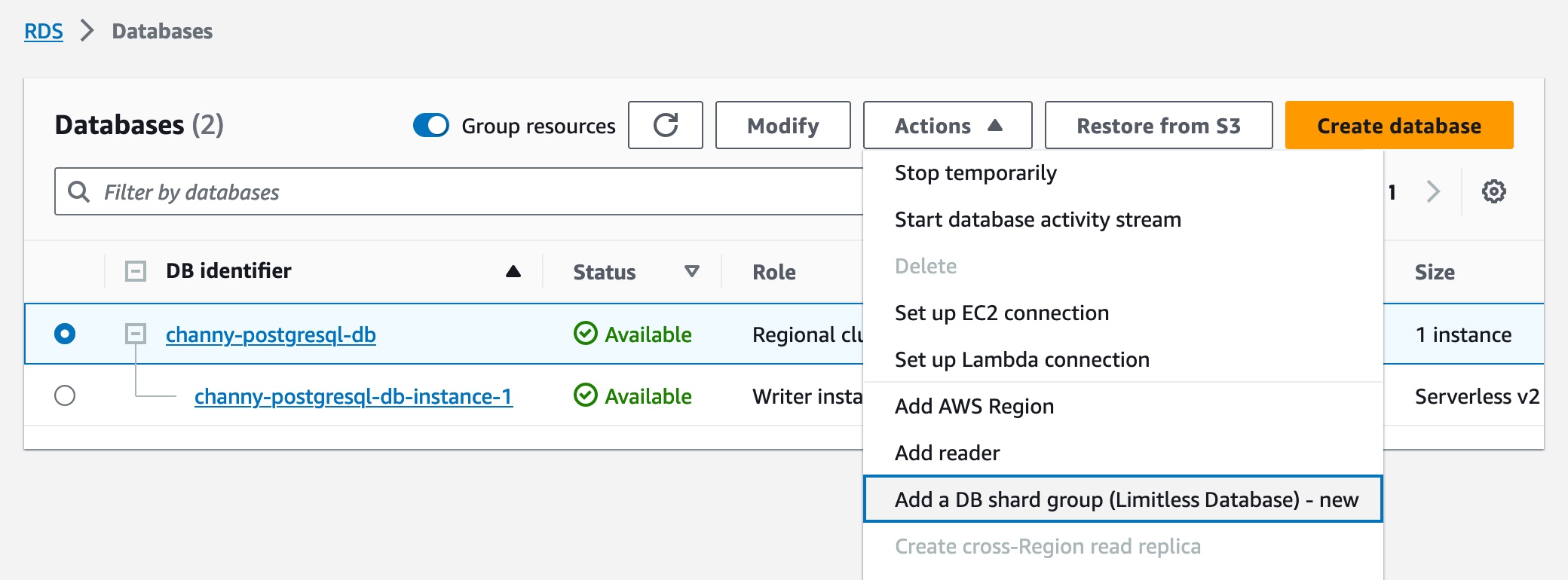
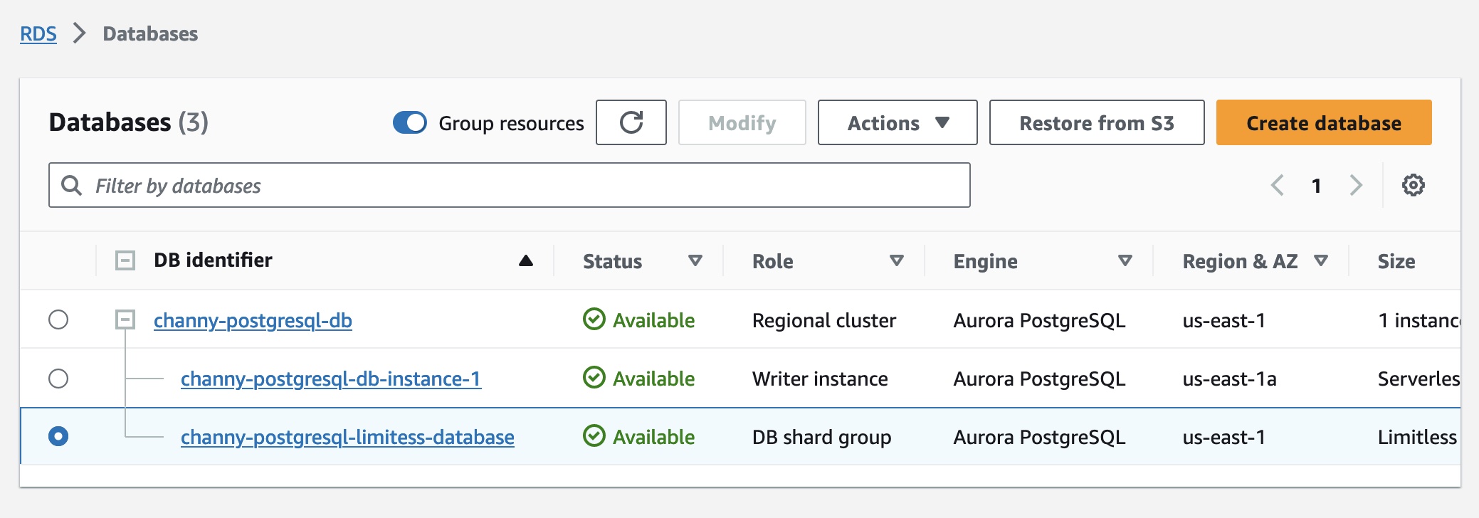


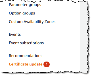 Don’t be surprised if you have seen the Certificate Update in the


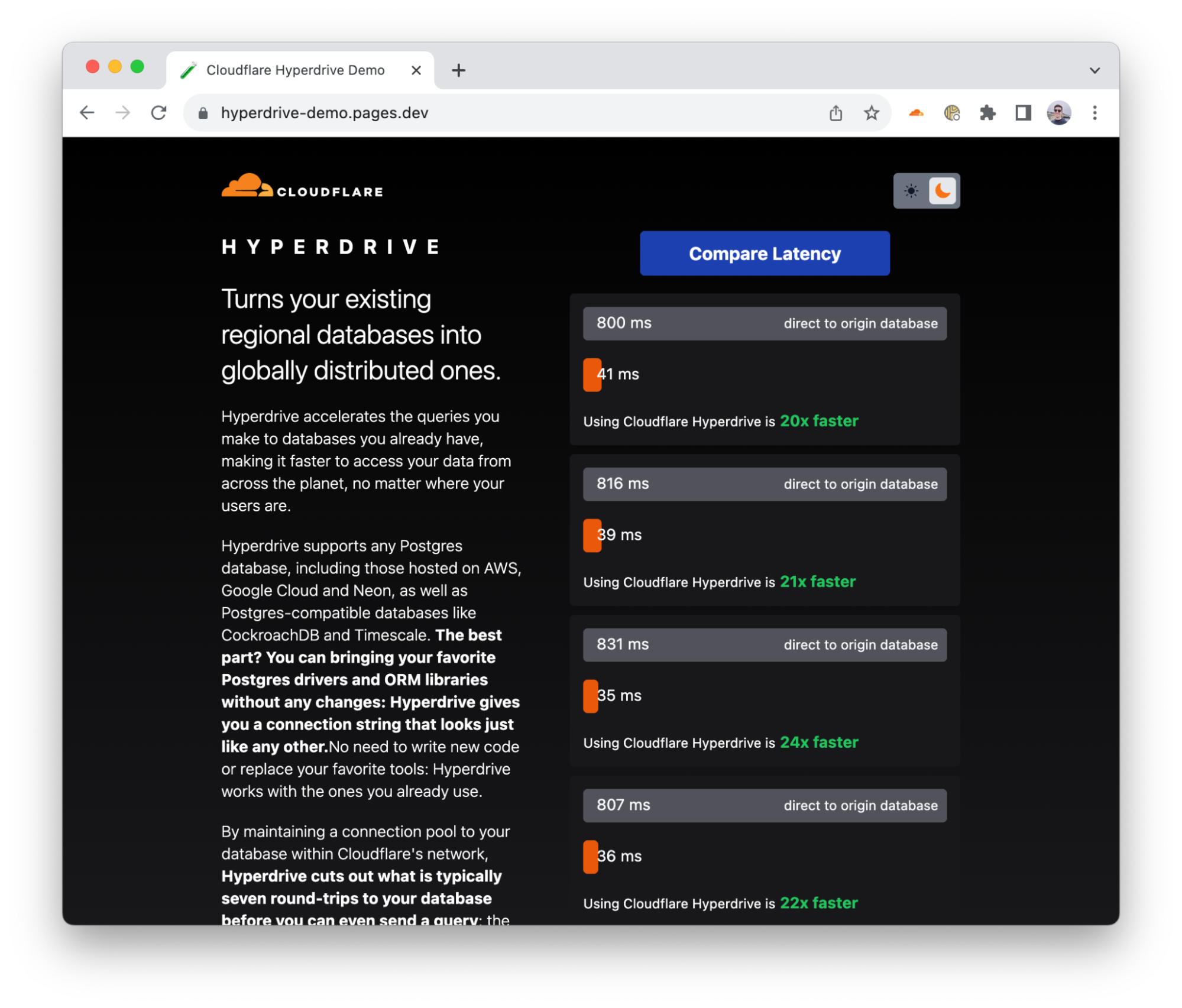
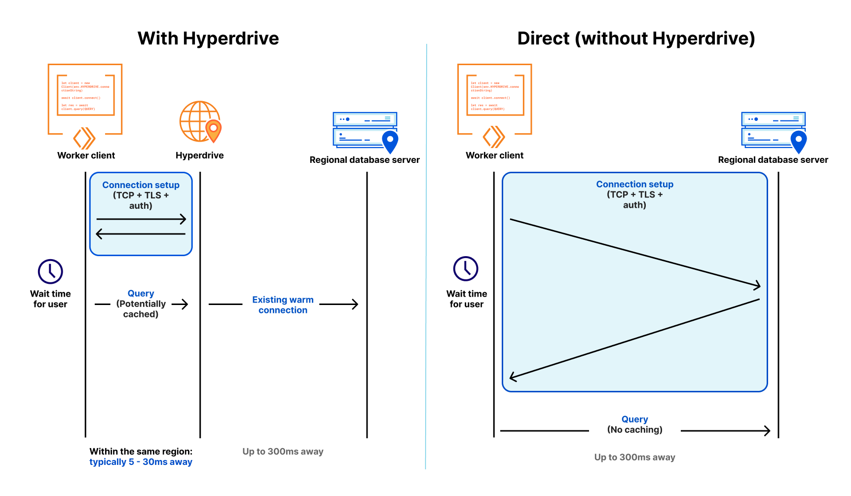


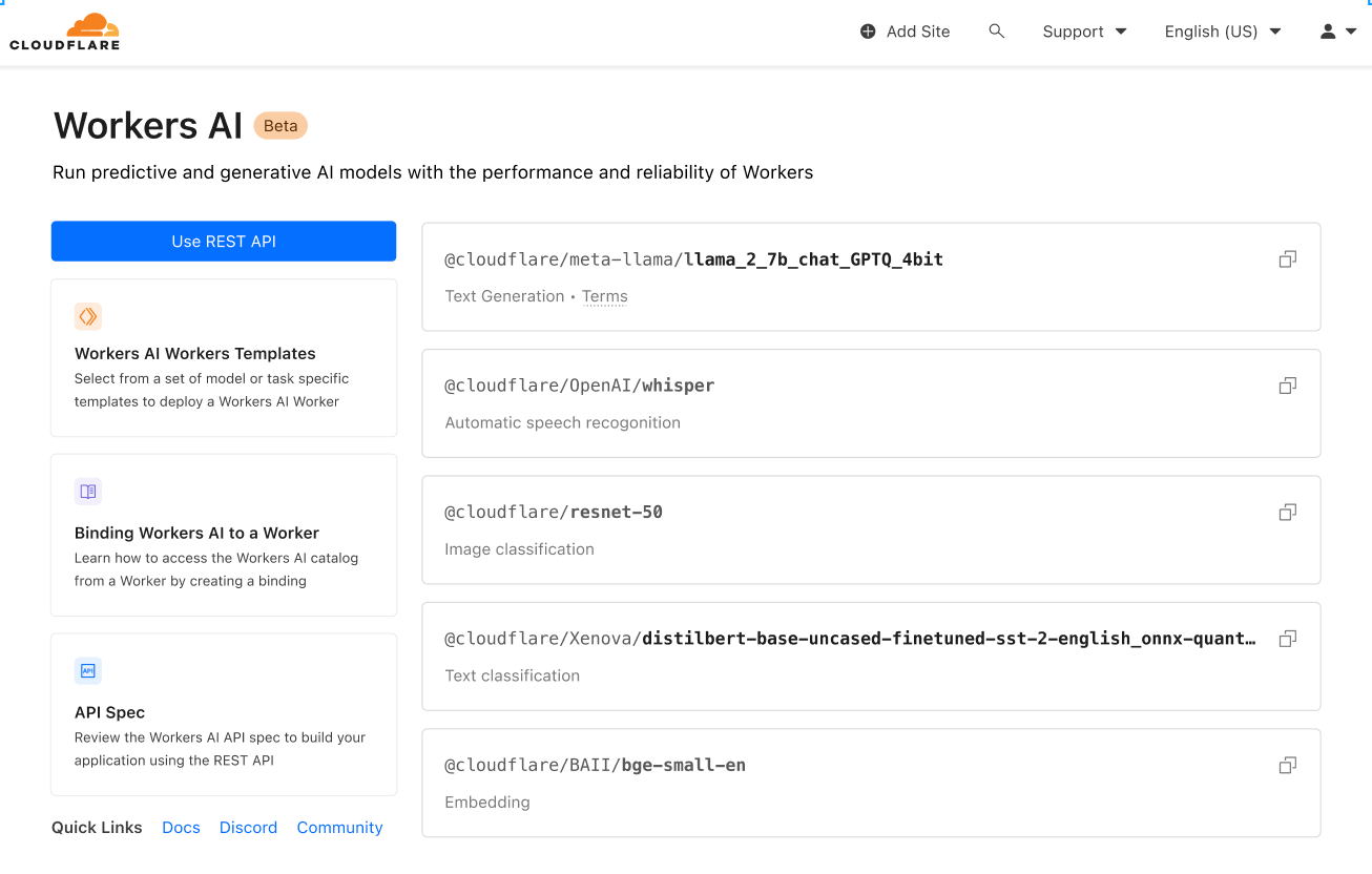


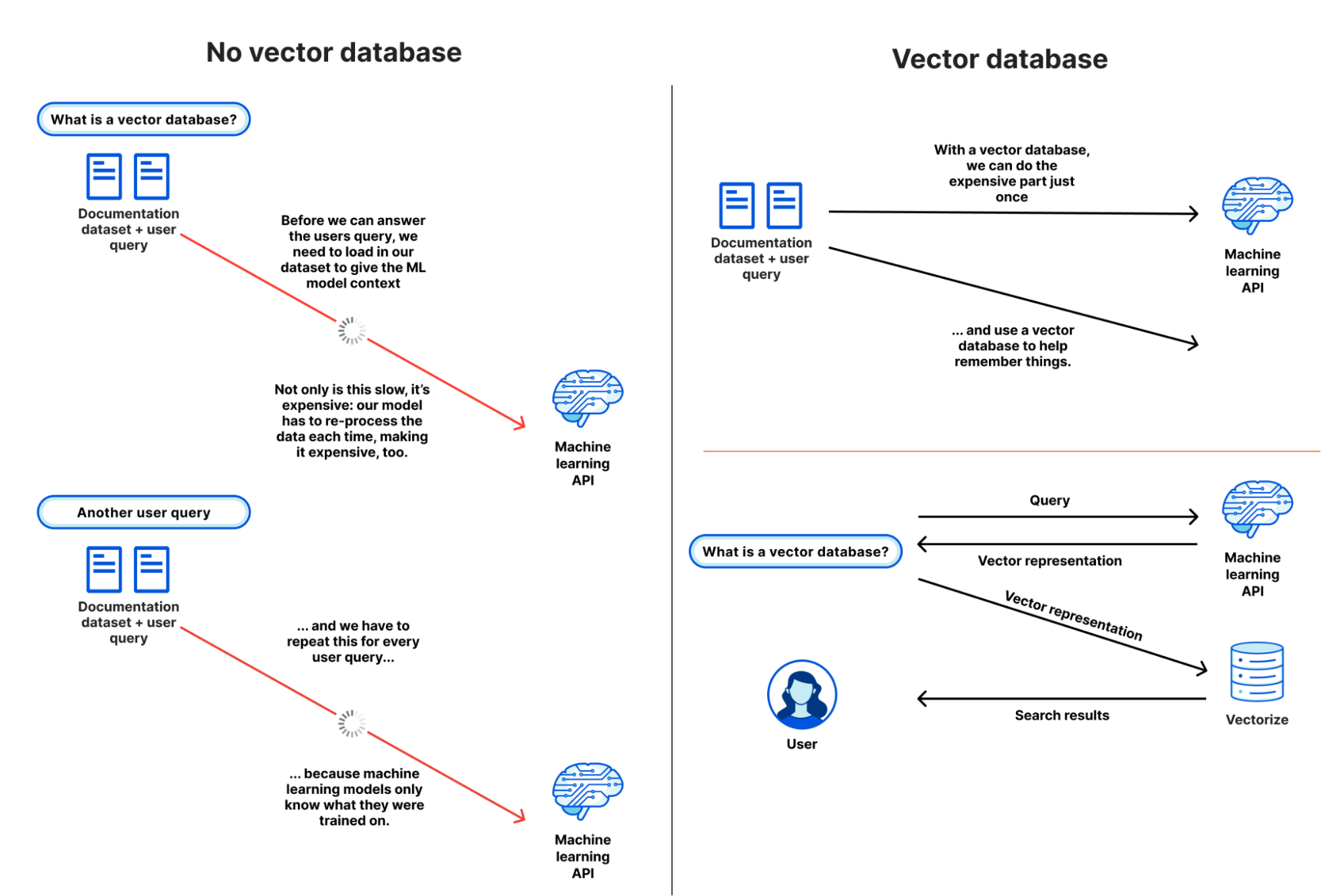
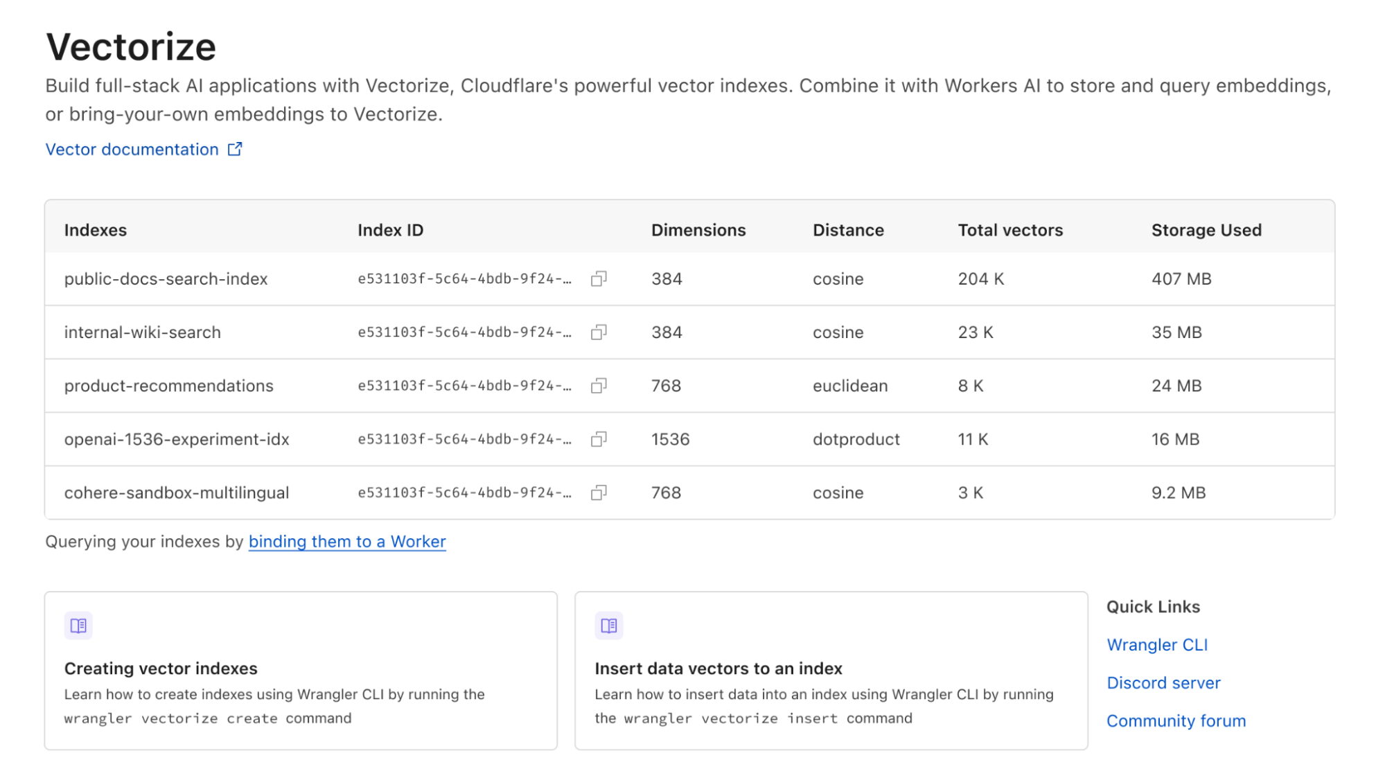


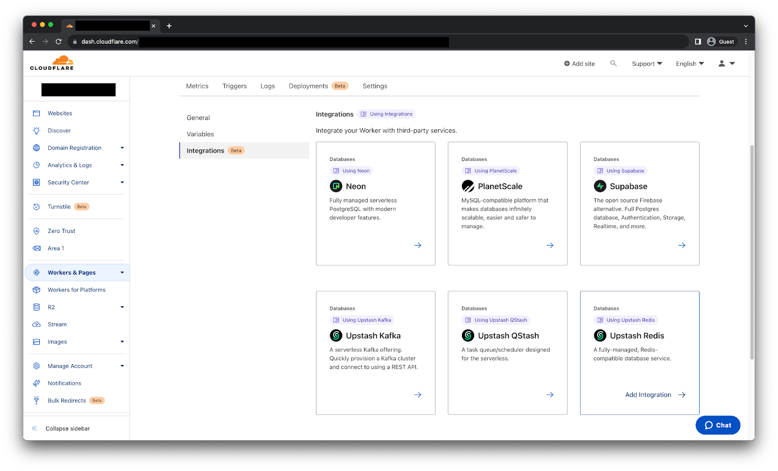
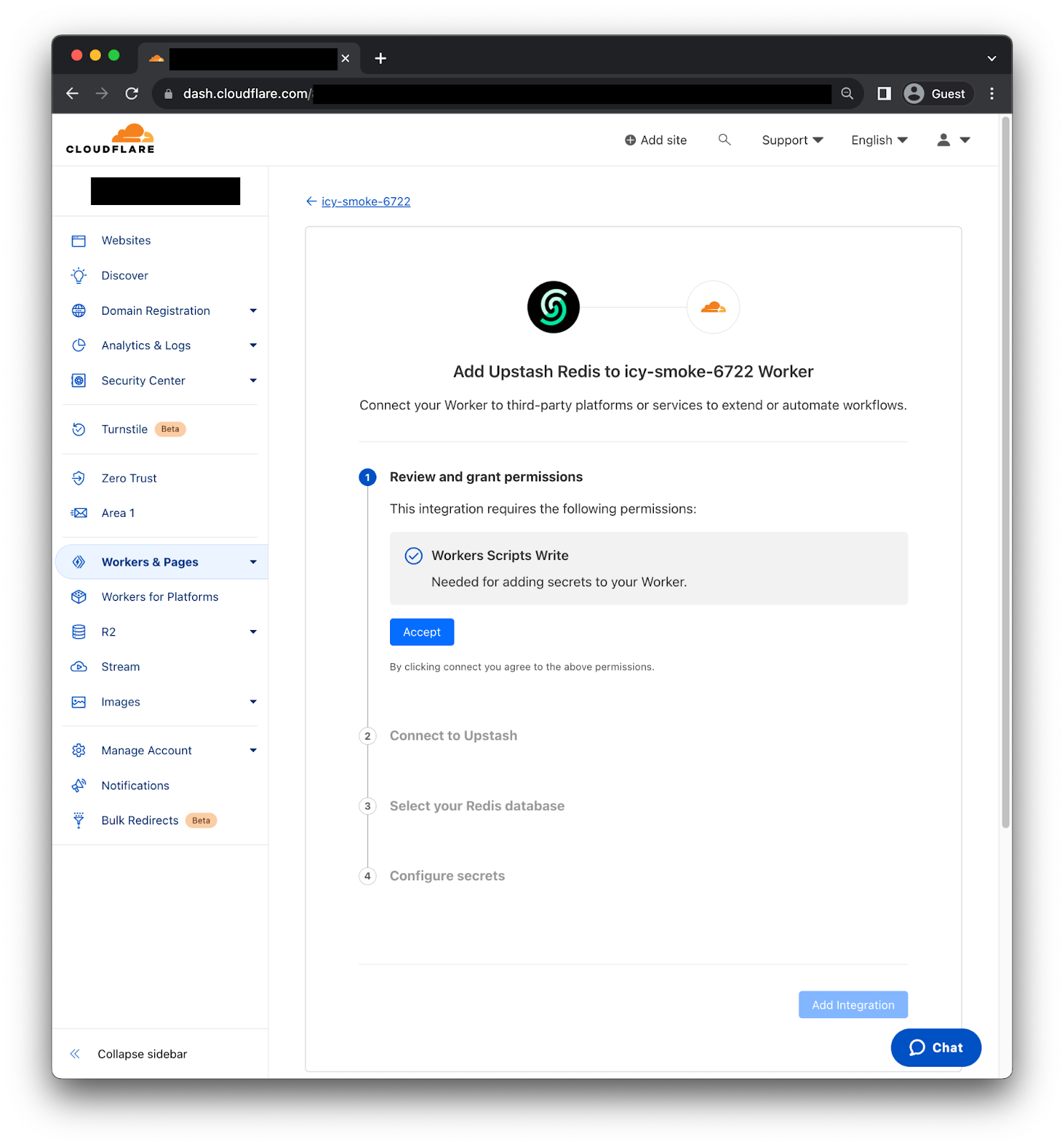


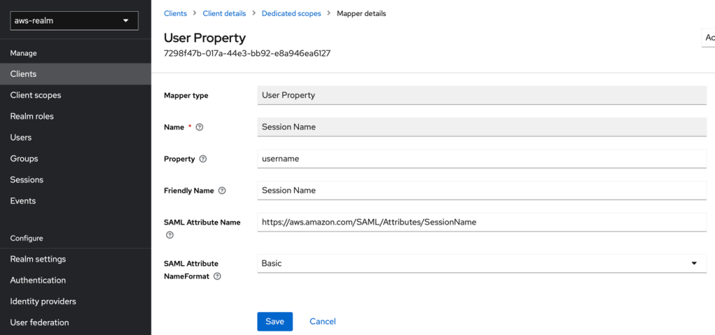


 Ayah Chamseddin is a Sr. Engagement Manager at AWS. She has a deep understanding of cloud technologies and has successfully overseen and lead strategic projects, partnering with clients to define business objectives, develop implementation strategies, and drive the successful delivery of solutions.
 Vamsi Bhadriraju is a Data Architect at AWS. He works closely with enterprise customers to build data lakes and analytical applications on the AWS Cloud.
 Srikanth Baheti is a Specialized World Wide Principal Solutions Architect for Amazon QuickSight. He started his career as a consultant and worked for multiple private and government organizations. Later he worked for PerkinElmer Health and Sciences & eResearch Technology Inc, where he was responsible for designing and developing high traffic web applications, highly scalable and maintainable data pipelines for reporting platforms using AWS services and Serverless computing.
 Raji Sivasubramaniam is a Sr. Solutions Architect at AWS, focusing on Analytics. Raji is specialized in architecting end-to-end Enterprise Data Management, Business Intelligence and Analytics solutions for Fortune 500 and Fortune 100 companies across the globe. She has in-depth experience in integrated healthcare data and analytics with wide variety of healthcare datasets including managed market, physician targeting and patient analytics.