Tag Archives: Amazon EC2

Building a Cloud in the Cloud: Running Apache CloudStack on Amazon EC2, Part 2

Post Syndicated from Sheila Busser original https://aws.amazon.com/blogs/compute/building-a-cloud-in-the-cloud-running-apache-cloudstack-on-amazon-ec2-part-2/

This blog is written by Mark Rogers, SDE II – Customer Engineering AWS.

In part 1, I showed you how to run Apache CloudStack with KVM on a single Amazon Elastic Compute Cloud (Amazon EC2) instance. That simple setup is great for experimentation and light workloads. In this post, things will get a lot more interesting. I’ll show you how to create an overlay network in your Amazon Virtual Private Cloud (Amazon VPC) that allows CloudStack to scale horizontally across multiple EC2 instances. This same method could work with other hypervisors, too.

If you haven’t read it yet, then start with part 1. It explains why this network setup is necessary. The same prerequisites apply to both posts.

Making things easier

I wrote some scripts to automate the CloudStack installation and OS configuration on CentOS 7. You can customize them to meet your needs. I also wrote some AWS CloudFormation templates you can copy in order to create a demo environment. The README file has more details.

The scalable method

Our team started out using a single EC2 instance, as described in my last post. That worked at first, but it didn’t have the capacity we needed. We were limited to a couple of dozen VMs, but we needed hundreds. We also needed to scale up and down as our needs changed. This meant we needed the ability to add and remove CloudStack hosts. Using a Linux bridge as a virtual subnet was no longer adequate.

To support adding hosts, we need a subnet that spans multiple instances. The solution I found is Virtual Extensible LAN (VXLAN). It’s lightweight, easy to configure, and included in the Linux kernel. VXLAN creates a layer 2 overlay network that abstracts away the details of the underlying network. It allows machines in different parts of a network to communicate as if they’re all attached to the same simple network switch.

Another example of an overlay network is an Amazon VPC. It acts like a physical network, but it’s actually a layer on top of other networks. It’s networks all the way down. VXLAN provides a top layer where CloudStack can sit comfortably, handling all of your VM needs, blissfully unaware of the world below it.

An overlay network comes with some big advantages. The biggest improvement is that you can have multiple hosts, allowing for horizontal scaling. Having more hosts not only gives you more computing power, but also lets you do rolling maintenance. Instead of putting the database and file storage on the management server, I’ll show you how to use Amazon Elastic File System (Amazon EFS) and Amazon Relational Database Service (Amazon RDS) for scalable and reliable storage.

EC2 Instances

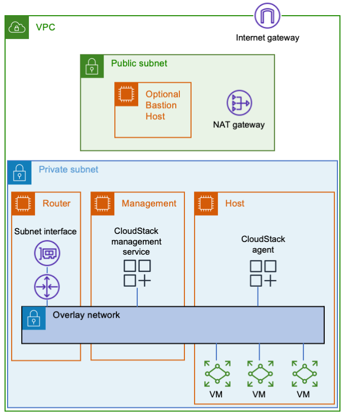
Let’s start with three Amazon EC2 instances. One will be a router between the overlay network and your Amazon VPC, the second one will be your CloudStack management server, and the third one will be your VM host. You’ll also need a way to connect to your instances, such as a bastion host or a VPN endpoint.

Three EC2 instances are connected to an AWS subnet. There's an overlay network that spans all three instances.The router instance connects the overlay network to the AWS subnet. The management instance contains the CloudStack management service, which is attached to the overlay network. The host instance contains the CloudStack agent and some VMs, all of which are connected to the overlay network.VXLAN must send and receive multicast traffic. Only Nitro instances can be multicast senders. As you plan, look at the list of Nitro instance types.

The router won’t need much computing power, but it will need enough network bandwidth to meet your needs. If you put Amazon EFS in the same subnet as your instances, then they’ll communicate with it directly, thereby reducing the load on the router. Decide how much network throughput you want, and then pick a suitable Nitro instance type.

After creating the router instance, configure AWS to use it as a router. Stop source/destination checking in the instance’s network settings. Then update the applicable AWS route tables to use the router as the target for the overlay network. The router’s security group needs to allow ingress to the CloudStack UI (TCP port 8080) and any services you plan to offer from VMs.

For the management server, you’ll want a Nitro instance type. It’s going to use more CPU than your router, so plan accordingly.

In addition to being a Nitro type, the host instance must also be a metal type. Metal instances have hardware virtualization support, which is needed by KVM. If you have a new AWS account with a low on-demand vCPU limit, then consider starting with an m5zn.metal, which has 48 vCPUs. Otherwise, I suggest going directly to a c5.metal because it provides 96 vCPUs for a similar price. There are bigger types available depending on your compute needs, budget, and vCPU limit. If your account’s on-demand vCPU limit is too low, then you can file a support ticket to have it raised.

Networking

All of the instances should be on a dedicated subnet. Sharing the subnet with other instances can cause communication issues. For an example, refer to the following figure. The subnet has an instance named TroubleMaker that’s not on the overlay network. If TroubleMaker sends a request to the management instance’s overlay network address, then here’s what happens:

  1. The request goes through the AWS subnet to the router.
  2. The router forwards the request via the overlay network.
  3. The CloudStack management instance has a connection to the same AWS subnet that TroubleMaker is on. Therefore, it responds directly instead of using the router. This isn’t the return path that AWS is expecting, so the response is dropped.

This diagram depicts the steps described in the previous paragraph.

If you move TroubleMaker to a different subnet, then the requests and responses will all go through the router. That will fix the communication issues.

The instances in the overlay network will use special interfaces that serve as VXLAN tunnel endpoints (VTEPs). The VTEPs must know how to contact each other via the underlay network. You could manually give each instance a list of all of the other instances, but that’s a maintenance nightmare. It’s better to let the VTEPs discover each other, which they can do using multicast. You can add multicast support using AWS Transit Gateway.

Here are the steps to make VXLAN multicasts work:

  1. Enable multicast support when you create the transit gateway.
  2. Attach the transit gateway to your subnet.
  3. Create a transit gateway multicast domain with IGMPv2 support enabled.
  4. Associate the multicast domain with your subnet.
  5. Configure the eth0 interface on each instance to use IGMPv2. The following sample code shows how to do this.
  6. Make sure that your instance security groups allow ingress for IGMP queries (protocol 2 traffic from 0.0.0.0/32) and VXLAN traffic (UDP port 4789 from the other instances).

CloudStack VMs must connect to the same bridge as the VXLAN interface. As mentioned in the previous post, CloudStack cares about names. I recommend giving the interface a name starting with “eth”. Moreover, this naming convention tells CloudStack which bridge to use, thereby avoiding the need for a dummy interface like the one in the simple setup.

The following snippet shows how I configured the networking in CentOS 7. You must provide values for these variables:

  • $overlay_host_ip_address, $overlay_netmask, and $overlay_gateway_ip: Use values for the overlay network that you’re creating.
  • $dns_address: I recommend using the base of the VPC IPv4 network range, plus two. You shouldn’t use 169.654.169.253 because CloudStack reserves link-local addresses for its own use.
  • $multicast_address: The multicast address that you want VXLAN to use. Pick something in the multicast range that won’t conflict with anything else. I recommend choosing from the IPv4 local scope (239.255.0.0/16).
  • $interface_name: The name of the interface VXLAN should use to communicate with the physical network. This is typically eth0.

A couple of the steps are different for the router instance than for the other instances. Pay attention to the comments!

yum install -y bridge-utils net-tools

# IMPORTANT: Omit the GATEWAY setting on the router instance!
cat << EOF > /etc/sysconfig/network-scripts/ifcfg-cloudbr0
DEVICE=cloudbr0
TYPE=Bridge
ONBOOT=yes
BOOTPROTO=none
IPV6INIT=no
IPV6_AUTOCONF=no
DELAY=5
STP=no
USERCTL=no
NM_CONTROLLED=no
IPADDR=$overlay_host_ip_address
NETMASK=$overlay_netmask
DNS1=$dns_address
GATEWAY=$overlay_gateway_ip
EOF

cat << EOF > /sbin/ifup-local
#!/bin/bash
# Set up VXLAN once cloudbr0 is available.
if [[ \$1 == "cloudbr0" ]]
then
    ip link add ethvxlan0 type vxlan id 100 dstport 4789 group "$multicast_address" dev "$interface_name"
    brctl addif cloudbr0 ethvxlan0
    ip link set up dev ethvxlan0
fi
EOF

chmod +x /sbin/ifup-local

# Transit Gateway requires IGMP version 2
echo "net.ipv4.conf.$interface_name.force_igmp_version=2" >> /etc/sysctl.conf
sysctl -p

# Enable IPv4 forwarding
# IMPORTANT: Only do this on the router instance!
echo 'net.ipv4.ip_forward=1' >> /etc/sysctl.conf
sysctl -p

# Restart the network service to make the changes take effect.
systemctl restart network

Storage

Let’s look at storage. Create an Amazon RDS database using the MySQL 8.0 engine, and set a master password for CloudStack’s database setup tool to use. Refer to the CloudStack documentation to find the MySQL settings that you’ll need. You can put the settings in an RDS parameter group. In case you’re wondering why I’m not using Amazon Aurora, it’s because CloudStack needs the MyISAM storage engine, which isn’t available in Aurora.

I recommend Amazon EFS for file storage. For efficiency, create a mount target in the subnet with your EC2 instances. That will enable them to communicate directly with the mount target, thereby bypassing the overlay network and router. Note that the system VMs will use Amazon EFS via the router.

If you want, you can consolidate your CloudStack file systems. Just create a single file system with directories for each zone and type of storage. For example, I use directories named /zone1/primary, /zone1/secondary, /zone2/primary, etc. You should also consider enabling provisioned throughput on the file system, or you may run out of bursting credits after booting a few VMs.

One consequence of the file system’s scalability is that the amount of free space (8 exabytes) will cause an integer overflow in CloudStack! To avoid this problem, reduce storage.overprovisioning.factor in CloudStack’s global settings from 2 to 1.

When your environment is ready, install CloudStack. When it asks for a default gateway, remember to use the router’s overlay network address. When you add a host, make sure that you use the host’s overlay network IP address.

Cleanup

If you used my CloudFormation template, delete the stack and remove any route table entries you added.

If you didn’t use CloudFormation, here are the things to delete:

  1. The CloudStack EC2 instances
  2. The Amazon RDS database and parameter group
  3. The Amazon EFS file system
  4. The transit gateway multicast domain subnet association
  5. The transit gateway multicast domain
  6. The transit gateway VPC attachment
  7. The transit gateway
  8. The route table entries that you created
  9. The security groups that you created for the instances, database, and file system

Conclusion

The approach I shared has many steps, but they’re not bad when you have a plan. Whether you need a simple setup for experiments, or you need a scalable environment for a data center migration, you now have a path forward. Give it a try, and comment here about the things you learned. I hope you find it useful and fun!

“Apache”, “Apache CloudStack”, and “CloudStack” are trademarks of the Apache Software Foundation.

Building a Cloud in the Cloud: Running Apache CloudStack on Amazon EC2, Part 1

Post Syndicated from Sheila Busser original https://aws.amazon.com/blogs/compute/building-a-cloud-in-the-cloud-running-apache-cloudstack-on-amazon-ec2-part-1/

This blog is written by Mark Rogers, SDE II – Customer Engineering AWS.

How do you put a cloud inside another cloud? Some features that make Amazon Elastic Compute Cloud (Amazon EC2) secure and wonderful also make running CloudStack difficult. The biggest obstacle is that AWS and CloudStack both want to manage network resources. Therefore, we must keep them out of each other’s way. This requires some steps that aren’t obvious, and it took a long time to figure out. I’m going to share what I learned, so that you can navigate the process more easily.

Apache CloudStack is an open-source platform for deploying and managing virtual machines (VMs) and the associated network and storage infrastructure. You would normally run it on your own hardware to create your own cloud. But there can be advantages to running it inside of an Amazon Virtual Private Cloud (Amazon VPC), including how it could help you migrate out of a data center. It’s a great way to create disposable environments for experiments or training. Furthermore, it’s a convenient way to test-drive the new CloudStack support in Amazon Elastic Kubernetes Service (Amazon EKS) Anywhere. In my case, I needed to create development and test environments for a project that uses the CloudStack API. The environments needed to be shared and scalable. Our build pipelines were already in AWS, so it made sense to put the new environments there, too.

CloudStack can work with a number of hypervisors. The instructions in this article will use Kernel-based Virtual Machine (KVM) on Linux. KVM will manage the VMs at a low level, and CloudStack will manage KVM.

Prerequisites

Most of the information in this article should be applicable to a range of CloudStack versions. I targeted CloudStack 4.14 on CentOS 7. I also tested CloudStack versions 4.16 and 4.17, and I recommend them.

The official CentOS 7 x86_64 HVM image works well. If you use a different Linux flavor or version, then you might have to modify some of the implementation details.

You’ll need to know the basics of CloudStack. The scope of this article is making CloudStack and AWS coexist peacefully. Once CloudStack is running, I’m assuming that you’ll handle things from there.  Refer to the AWS documentation and CloudStack documentation for information on security and other best practices.

Making things easier

I wrote some scripts to automate the installation. You can run them on EC2 instances with CentOS 7, and they’ll do all the installation and OS configuration for you. You can use them as they are, or customize them to meet your needs. I also wrote some AWS CloudFormation templates you can copy in order to create a demo environment. The README file has more details.

Amazon EC2 instance types

KVM requires hardware virtualization support. Most EC2 instances are VMs that don’t support nested virtualization. To get access to the bare hardware, you need a metal instance type.

I like c5.metal because it’s one of the least expensive metal types, and has a low cost per vCPU. It has 96 vCPUs and 192 GiB of memory. If you run 20 VMs on it, with 4 CPU cores and 8 GiB of memory each, then you’d still have 16 vCPUs and 32 GiB to share between the operating system, CloudStack, and MySQL. Using CloudStack’s overprovisioning feature, you could fit even more VMs if they’re running light loads.

Networking

The biggest challenge is the network. AWS knows which IP and MAC addresses should exist, and it knows the machines to which they should belong. It blocks any traffic that doesn’t fit its idea of how the network should behave. Simultaneously, CloudStack assumes that any IP or MAC address it invents should work just fine. When CloudStack assigns addresses to VMs on an AWS subnet, their network traffic gets blocked.

You could get around this by enabling network address translation (NAT) on the instance running CloudStack. That’s a great solution if it fits your needs, but it makes it hard for other machines in your Amazon VPC to contact your VMs. I recommend a different approach.

Although AWS restricts what you can do with its layer 2 network, it’s perfectly happy to let you run your own layer 3 router. Your EC2 instance can act as a router to a new virtual subnet that’s outside of the jurisdiction of AWS. The instance integrates with AWS just like a VPN appliance, routing traffic to wherever it needs to go. CloudStack can do whatever it wants in the virtual subnet, and everybody’s happy.

What do I mean by a virtual subnet? This is a subnet that exists only inside the EC2 instance.  It consists of logical network interfaces attached to a Linux bridge. The entire subnet exists inside a single EC2 instance. It doesn’t scale well, but it’s simple. In my next post, I’ll cover a more complicated setup with an overlay network that spans multiple instances to allow horizontal scaling.

The simple way

The simple way is to put everything in one EC2 instance, including the database, file storage, and a virtual subnet. Because everything’s stored locally, allocate enough disk space for your needs. 500 GB will be enough to support a few basic VMs. Create or select a security group for your instance that gives users access to the CloudStack UI (TCP port 8080). The security group should also allow access to any services that you’ll offer from your VMs.

EC2 instance summary info showing 1 instance, CentOS 7 (x86_64) AMI, c5.metal instance type, a security group name, and a 500 GiB volume

When you have your instance, configure AWS to treat it as a router.

  1. Go to Amazon EC2 in the AWS Management Console.
  2. Select your instance, and stop source/destination checking.

In the EC2 Actions menu, select Networking, then Change source/destination check.

3. Update the subnet route tables.

a. Go to the VPC settings, and select Route Tables.

b. Identify the tables for subnets that need CloudStack access.

c. In each of these tables, add a route to the new virtual subnet. The route target should be your EC2 instance.

4. Depending on your network needs, you may also need to add routes to transit gateways, VPN endpoints, etc.

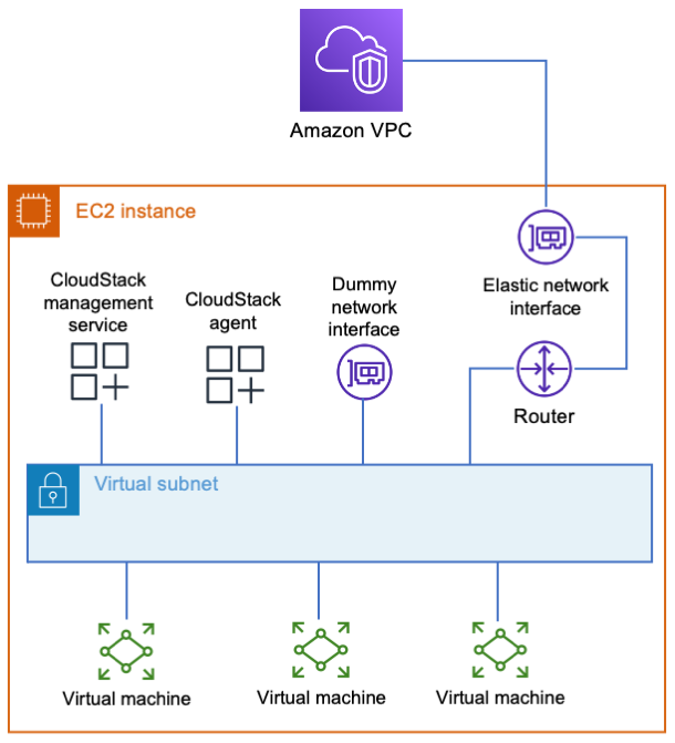
Because everything will be on one server, creating a virtual subnet is simply a matter of creating a Linux bridge. CloudStack must find a network adapter attached to the bridge. Therefore, add a dummy interface with a name that CloudStack will recognize.

A single EC2 instance contains the CloudStack management service, the CloudStack agent, a dummy network interface, several virtual machines, and a router. All of those things are connected to each other by a virtual subnet that exists inside the instance. The instance's elastic network interface is connected between the router and the Amazon VPC.The following snippet shows how I configure networking in CentOS 7. You must provide values for the variables $virutal_host_ip_address and $virtual_netmask to reflect the virtual subnet that you want to create. For $dns_address, I recommend the base of the VPC IPv4 network range, plus two. You shouldn’t use 169.654.169.253 because CloudStack reserves link-local addresses for its own use.

yum install -y bridge-utils net-tools

# The bridge must be named cloudbr0.

cat << EOF > /etc/sysconfig/network-scripts/ifcfg-cloudbr0
DEVICE=cloudbr0
TYPE=Bridge
ONBOOT=yes
BOOTPROTO=none
IPV6INIT=no
IPV6_AUTOCONF=no
DELAY=5
STP=yes
USERCTL=no
NM_CONTROLLED=no
IPADDR=$virtual_host_ip_address
NETMASK=$virtual_netmask
DNS1=$dns_address
EOF

# Create a dummy network interface.
cat << EOF > /etc/sysconfig/modules/dummy.modules
#!/bin/sh
/sbin/modprobe dummy numdummies=1
/sbin/ip link set name ethdummy0 dev dummy0
EOF

chmod +x /etc/sysconfig/modules/dummy.modules
/etc/sysconfig/modules/dummy.modules

cat << EOF > /etc/sysconfig/network-scripts/ifcfg-ethdummy0
TYPE=Ethernet
BOOTPROTO=none
NAME=ethdummy0
DEVICE=ethdummy0
ONBOOT=yes
BRIDGE=cloudbr0
NM_CONTROLLED=no
EOF

# Turn the instance into a router

echo 'net.ipv4.ip_forward=1' >> /etc/sysctl.conf
sysctl -p

# Must kill dhclient or the network service won't restart properly.
# A reboot would also work, if you’d rather do that.

pkill dhclient
systemctl restart network

CloudStack must know which IP addresses to use for inter-service communication. It will select by resolving the machine’s fully qualified domain name (FQDN) to an address. The following commands will make it to choose the right one. You must provide a value for $virtual_host_ip_address.

hostnamectl set-hostname cloudstack.localdomain

echo "$virtual_host_ip_address cloudstack.localdomain" >> 
/etc/hosts

You can finish the setup by following the Quick Installation Guide.

Remember that CloudStack is only directly connected to your virtual network. The EC2 instance is the router that connects the virtual subnet to the Amazon VPC. When you’re configuring CloudStack, use your instance’s virtual subnet address as the default gateway.

Use the EC2 instance's virtual subnet IP address as the default gateway in CloudStack. In this example, the virtual subnet is 10.100.0.0/16, and the instance's address in that subnet is 10.100.0.1. CloudStack then uses 10.100.0.1 as the default gateway.

To access CloudStack from your workstation, you’ll need a connection to your VPC. This can be through a client VPN or a bastion host. If you use a bastion, its subnet needs a route to your virtual subnet, and you’ll need an SSH tunnel for your browser to access the CloudStack UI. The UI is at http://x.x.x.x:8080/client/, where x.x.x.x is your CloudStack instance’s virtual subnet address. Note that CloudStack’s console viewer won’t work if you’re using an SSH tunnel.

If you’re just experimenting with CloudStack, then I suggest saving money by stopping your instance when it isn’t needed. The safe way to do that is:

  1. Disable your zone in the CloudStack UI.
  2. Put the primary storage into maintenance mode.
  3. Wait for the switch to maintenance mode to be complete.
  4. Stop the EC2 instance.

When you’re ready to turn everything back on, simply reverse those steps. If you have any virtual routers in CloudStack, then you may need to start those, too.

Cleanup

If you used my CloudFormation template, then delete the stack and remove any route table entries you added. If you didn’t use CloudFormation, then terminate the EC2 instance, delete the security group you created for it, and remove any route table entries that you added.

Conclusion

Getting CloudStack to run on AWS isn’t so bad. The hardest part is simply knowing how. The setup explained here is great for small installations, but it can only scale vertically. In my next post, I’ll show you how to create an installation that scales horizontally. Instead of using a virtual subnet that exists in a single EC2 instance, we’ll build an overlay network that spans multiple instances. It will use more components and features, including some that might be new to you. I hope you find it interesting!

Now that you can create a simple setup, give it a try! I hope you have fun and learn something new along the way. Comment with the results of your experiments.

“Apache”, “Apache CloudStack”, and “CloudStack” are trademarks of the Apache Software Foundation.

Deploying Oracle RAC in AWS Outposts via FlashGrid Cluster

Post Syndicated from Andreas Bogner original https://aws.amazon.com/blogs/architecture/deploying-oracle-rac-in-aws-outposts-via-flashgrid-cluster/

Amazon Web Services (AWS) customers are deploying AWS Outposts as a fully managed solution that delivers AWS infrastructure and services to on-premises or edge locations for a truly consistent hybrid experience. Those hybrid cloud workloads can require highly available Oracle databases running on- or close-to premises. One way to meet this requirement is Oracle Real Application Clusters (RAC) on top of two or more AWS Outposts racks using the FlashGrid Cluster solution.

In this post, we follow up on a Marketplace blog that describes how to deploy Oracle RAC via FlashGrid Cluster in the AWS regions. Deploying the solution onto AWS Outposts requires additional steps as the Outpost racks communicate between VPCs and across the on-premises network. In the following we explain how to configure the network for a multi-Outpost setup, how to deploy FlashGrid Cluster with Oracle RAC, and how to connect to the database cluster from the on-premises network.

Solution overview

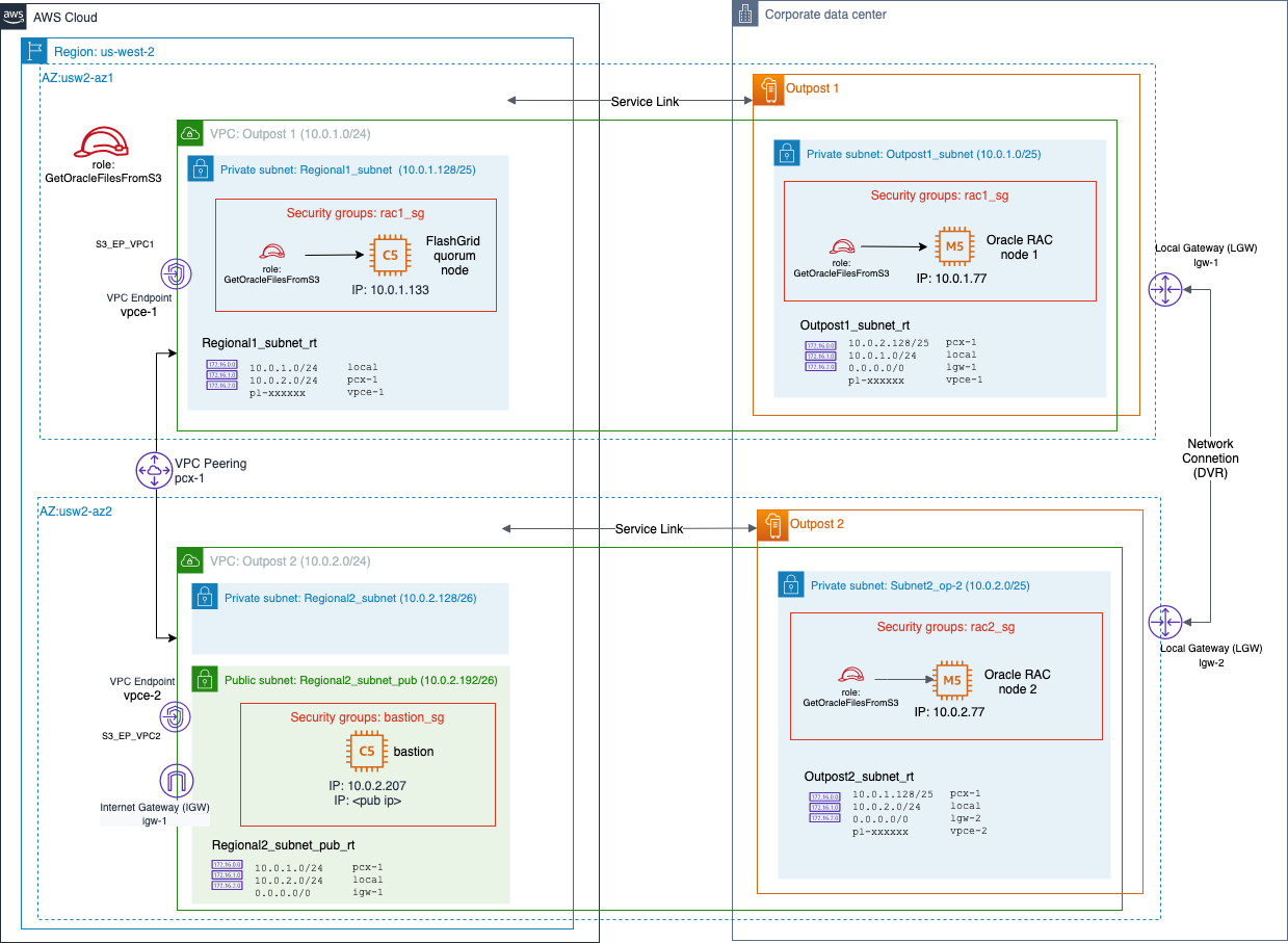
This architecture uses two logical Outposts (42U racks) that are connected to different Availability Zones (AZs) in the same region for high availability. The networking is configured such that the communication between Amazon Elastic Compute Cloud (Amazon EC2) instances on two distinct Outpost racks uses Outpost’s local gateways and the corporate network. Therefore, data will not leave the premises unless explicitly copied to the Cloud region.

The FlashGrid Cluster solution deploys one node to each Outpost rack and an additional quorum node to the Cloud region. The cluster nodes provide the Oracle ASM disk groups and the Oracle RAC nodes. FlashGrid Cluster for Oracle RAC ensures that storage is replicated between nodes (Figure 1).

Architecture for a deployment across two logical AWS Outposts

Figure 1. Architecture for a deployment across two logical AWS Outposts

We provide a complete, step-by-step guide that deploys an Oracle RAC database across two Outpost racks.

It takes three steps to get your database up and running:

  1. Networking: prepare the virtual private clouds (VPCs), subnets, and route tables
  2. FlashGrid Cluster: use the FlashGrid Launcher to create an Oracle RAC cluster
  3. Database: configure Oracle RAC and connect to the database

The deployment uses a CloudFormation template that is generated based on the workload’s specific parameters.

Prerequisites

For this solution, you require:

Networking setup

A single VPC cannot span multiple Outposts. Therefore, each Outpost should have a separately configured VPC.

A security group allowing traffic between the nodes of the cluster must be created in each VPC. Private IP addresses of the other nodes in the cluster should be configured as allowed sources of the traffic. (A security group rule cannot reference a security group in a different VPC.)

The steps suggested for configuring the network, as in Figure 2:

  1. Create a VPC for each Outpost and a VPC between those VPCs. Ensure that the VPCs are associated with the respective local gateways on each Outpost.
  2. Within each VPC, create a subnet for the corresponding Outpost and a subnet in the Region. Add route tables to each Outpost subnet that allow cross-VPC routing (as in Table 1).Table 1. Main route table for VPC ‘Outpost 1’

    Destination Target
    10.0.1.0/24 local
    10.0.2.0/25 lgw-11111111111111111
    10.0.2.128/25 pcx-11223344556677889
    pl-12345678 vpce-12345678901234567
  3. For each of the cluster nodes, allocate a private IP address within the corresponding subnet.
  4. Within each VPC create a separate security group for each cluster. The security group must allow all inbound and outbound traffic from all nodes of the same cluster using their private IP addresses.
  5. Optional: Create a public subnet in the region in either one of the VPCs. Deploying a bastion host EC2 instance into this subnet will allow you to connect by SSH to the Oracle RAC nodes later.
  6. Open SSH access (TCP 22) and Oracle client access (default ports: TCP 1521, 1522) either by adding the corresponding rules to the same security groups or assigning additional security groups to all cluster node instances after the cluster deployment is complete.
  7. Create an Amazon Simple Storage Service (Amazon S3) gateway endpoint in each VPC and add corresponding routes. It is critical to use Amazon S3 gateway endpoints, otherwise the Oracle RAC nodes cannot download the installation binaries from the S3 bucket.
Setting up subnets on each Outpost via the AWS console

Figure 2. Setting up subnets on each Outpost via the AWS console

FlashGrid Cluster setup

The process of deploying FlashGrid Cluster consists of five main steps:

  1. Subscribing to a FlashGrid Cluster product in AWS Marketplace
  2. Uploading Oracle installation files to an S3 bucket in the Region
  3. Modifying the cluster configuration template with parameters specific to Outposts
  4. Using the FlashGrid Launcher tool to finalize cluster configuration and generate an AWS CloudFormation template
  5. Deploying the CloudFormation template

Subscribing to a FlashGrid Cluster product in AWS Marketplace

  1. Open one of the FlashGrid Cluster product pages in AWS Marketplace corresponding with the preferred operating system.
  2. Select Continue.
  3. Select the Manual Launch tab.
  4. Choose Accept Software Terms.

Creating an S3 bucket for Oracle installation files

During cluster provisioning, Oracle installation files are downloaded from an S3 bucket. The list of files that must be placed in the S3 bucket is displayed on the Oracle Files tab of the FlashGrid Launcher tool (next step). The S3 bucket is not supposed to have any sensitive data in it and can be hosted in any AWS Region. You can use the same bucket for multiple deployments.

To create an S3 bucket with the correct IAM role access:

  1. Create an S3 bucket or folder for uploading the installation files
  2. Within the IAM console, create a policy named GetOracleFilesFromS3, which allows the s3:GetObject action on all uploaded files
  3. Create an EC2 instance role named GetOracleFilesFromS3 and attach the GetOracleFilesFromS3 policy to it
  4. Use the GetOracleFilesFromS3 role when configuring cluster parameters in the FlashGrid Launcher
  5. Once the FlashGrid Launcher has provided a list of required Oracle installation files, place those into the S3 bucket

Modifying the cluster configuration template with parameters specific to Outposts

Download the configuration file template, and open it in a text editor. The template is for a two-node RAC cluster on Outposts in Multi-AZ configuration.

For the database node instances in the configuration file, manually set the following attributes:

  • outpost_arn: ARN of the target Outpost
  • ip: private IP address assigned to the EC2 instance
  • sg: security group ID
  • ins_type: instance type (ensure that this matches the available types for the Outposts)

Creating a cluster configuration file using FlashGrid Launcher tool

FlashGrid Launcher is an online tool that allows creating your desired configuration for the cluster and then generating a CloudFormation template for it.

  1. Open FlashGrid Launcher and upload the customized configuration file created at the previous step.
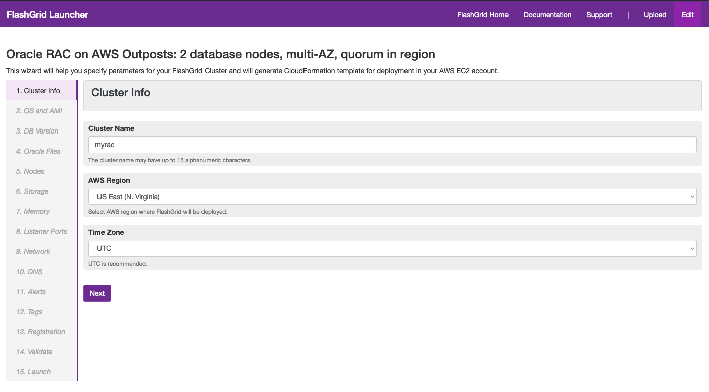
  2. Follow the step-by-step instructions in the Launcher tool (see Figure 3) until you get to the last Launch step.
    a. In the Oracle Files step, there is a list of installer files. Upload these files into the S3 bucket from the previous section (Creating an S3 bucket for Oracle installation files).
    b. In the Storage step, ignore the IOPS and MBPS parameters, as these parameters will not be used because Outposts uses the GP2 type of volumes.
    c. In the Network step, provide the Security Group ID that will be used for the quorum node located in the Region. Make sure to use a security group from the quorum node’s VPC.
  3. At the Launch step, click Launch FlashGrid. This generates a CloudFormation template and takes you to the AWS CloudFormation console.
The FlashGrid Launcher generates a CloudFormation template based on various input parameters

Figure 3. The FlashGrid Launcher generates a CloudFormation template based on various input parameters

Deploying the CloudFormation template

  1. Once you are in AWS CloudFormation console, select Next.
  2. Select the SSH key; do not change network parameters if you set them correctly in the Launcher. Select Next.
  3. On the Options page, if you added tags in FlashGrid Launcher, then do not add the same tags in CloudFormation console. You are free to add further tags in this step. Select Next.
  4. Select Create, and wait until the status of the stack changes to CREATE_COMPLETE.
  5. Connect by using SSH from the bastion host to the first cluster node as ec2-user with the SSH key you were provided when the stack was deployed.
  6. The welcome message details the current initialization status of the cluster: in progress, failed, or completed.
  7. If initialization is still in progress, wait for it to complete (this includes Oracle software installation and configuration). A broadcast message is delivered when initialization completes or fails. Cluster initialization takes 1 to 2 hours, depending on configuration.

Oracle database configuration

You can create an Oracle RAC database (or multiple databases) using Oracle DBCA tool and following standard Oracle best practices.

To connect to the Oracle RAC database using the SCAN listener, configure the Domain Name System (DNS) records and the connection string on client side:

  • On the DNS server(s) used by clients, add a record resolving to the VPC Private IP address of the node instance for each database node. In a test environment without a DNS server, the entries can be added to /etc/hosts on the clients instead of the DNS server.
  • In our example deployment, this is:
    rac1.example.com 10.0.1.77
    rac2.example.com 10.0.2.77
  • It is important that hostnames and domain names in the DNS records exactly match the hostnames as reported by the hostname command on the database servers.
  • Finally, define a connection string with the addresses of all database nodes listed:
    SCAN=
         (DESCRIPTION=
               (TRANSPORT_CONNECT_TIMEOUT=3) (RETRY_COUNT=6)
               (ADDRESS=(PROTOCOL=tcp) (HOST=rac2.example.com) (PORT=1521))
               (ADDRESS=(PROTOCOL=tcp) (HOST=rac2.example.com) (PORT=1521))
               (CONNECT_DATA=
                  (SERVER=DEDICATED)
                  (SERVICE_NAME=<service name>)
               )
          )

Visit the FlashGrid Help Center for more information on creating and connecting to a database.

Cleanup

The Oracle RAC instance together with the FlashGrid Cluster solution is deployed as a single CloudFormation stack. Deleting this stack will remove all associated resources, including the EBS volumes. Follow the approach detailed in the Delete Your Stacks But Keep Your Data blog post at the deployment stage to retain snapshots of all volumes automatically. You can also take snapshots of all EBS volumes manually before deleting the stack.

Conclusion

In this blog post, we have explored how to deploy Oracle RAC across two or more Outpost racks using FlashGrid Cluster. Running Oracle RAC on top of Outposts provides a highly available database solution for use cases that require you to run the workload on-premises, as in data-residency or latency-critical scenarios. Using the growing number of features for AWS Outposts rack, and you can more efficiently run hybrid workloads using the same tools and automation both in Cloud Regions and on-premises.

Further reading

An elastic deployment of Stable Diffusion with Discord on AWS

Post Syndicated from Steven Warren original https://aws.amazon.com/blogs/architecture/an-elastic-deployment-of-stable-diffusion-with-discord-on-aws/

Stable Diffusion is a state-of-the-art text-to-image model that generates images from text. Deploying text-to-image models such as Stable Diffusion can be difficult. Currently, Stable Diffusion requires specific computer hardware known as graphical processing units (GPUs). You can lower the bar to entry by offloading the text-to-image generation onto Amazon Web Services (AWS).

Discord is a popular voice, video, and text communication service. It provides a user interface that people can use to make text-to-image requests. When deployed, all members of a Discord server can create images by using Discord Slash Commands.

In this post, we discuss how to deploy a highly available solution on AWS. This solution will perform text-to-image generation with Stable Diffusion and use Discord as the user interface.

Solution architecture

Many of the services selected are serverless, which will offer many benefits. At the time of writing, Stable Diffusion requires a GPU for inference. Amazon Elastic Compute Cloud (Amazon EC2) was selected because it provides GPUs. The solution architecture is shown in the Figure 1.

Solution architecture diagram

Figure 1. Solution architecture diagram

Let us walk through the architecture of this solution.

Auto scaling with custom metrics

To properly scale the system, a custom Amazon CloudWatch metric is created. This custom CloudWatch metric calculates the number of Amazon Elastic Container Service (Amazon ECS) tasks required to adequately handle the amount of Amazon Simple Queue Service (Amazon SQS) messages. You should have a high-resolution CloudWatch metric to scale up quickly. For this use case, a high-resolution CloudWatch metric of every 10 seconds was implemented.

Next, let’s create the custom CW metric. Amazon EventBridge rules provide a serverless solution for starting actions on a schedule. Here we use an Amazon EventBridge rule, which initiates an AWS Step Function Express Workflow every minute. With the Express Workflow, we can create serverless workflows that take less than five minutes, which helps us avoid long running AWS Lambda functions. The Express Workflow runs a Lambda function every 10 seconds over a one-minute period, which generates the custom CloudWatch metric.

Two high-resolution CloudWatch alarms scale the system up and down, and are initiated by the custom CloudWatch metric. One CloudWatch alarm increases the ECS tasks and EC2 machines. The other alarm decreases the ECS tasks and EC2 machines.

Handling Discord requests

Someone on Discord sends a request. The Amazon API Gateway HTTP API receives the request and passes the information to an AWS Lambda function. The HTTP API provides a cost-effective option compared to REST APIs and provides tools for authentication and authorization. The HTTP API uses cross-origin resource sharing (CORS), which provides security because it only allows discord.com as an origin.

The AWS Lambda function provides a serverless solution for responding to the HTTP API requests. It transforms the HTTP API request and sends a message to the SQS First-In-First-Out (FIFO) queue. SQS seamelessly decouples the architecture between user requests and backend processing. A FIFO queue ensures that user requests are processed in the order they were requested. The AWS Lambda function sends a response back to the HTTP API within three seconds, which is a requirement of Discord Slash Commands.

When scaling up, an EC2 instance is registered with the ECS cluster. The EC2 instance type was selected because it provides GPU instances. ECS provides a repeatable solution to deploy the container across a variety of instance types. This solution currently only uses the g4dn.xlarge instance type. The ECS service will then place an ECS task onto the eligible EC2 instance. The ECS task will use the Amazon Elastic Container Registry (Amazon ECR) private registry to pull the image,  perform text-to-image processing, and respond to the Discord request. The ECR private registry is a managed container registry that manages the image.

Once there is an ECS task running on an Amazon EC2 instance, the ECS task will consume messages from the queue using long polling. This reduces the amount of ReceiveMessage requests the ECS task needs to send. When the ECS task receives a message from the queue, it will then processes the request.

Estimated monthly cost

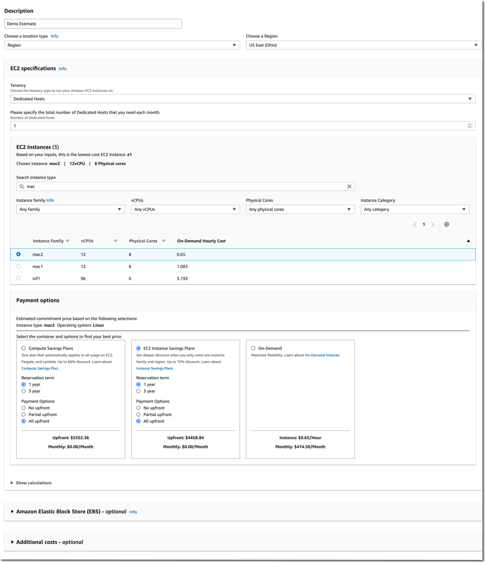
The example assumes 1,000 requests per month and each request takes 16 seconds to complete. Extra EC2 time was added for the time to begin processing messages (seven minutes) and auto scaling cooldown time (30 minutes). You can adjust the pricing calculations with the AWS Pricing Calculator to reflect your usage and estimated cost.

Prerequisites

This blog assumes familiarity with Terraform, Docker, Discord, Amazon EC2Amazon Elastic Block Store (Amazon EBS)Amazon Virtual Private Cloud (Amazon VPC), AWS Identity and Access Management (IAM), Amazon API Gateway, AWS Lambda, Amazon SQS, Amazon Elastic Container Registry (Amazon ECR), Amazon ECS, Amazon EventBridge, AWS Step Functions, and Amazon CloudWatch.

For this walkthrough, you should have the following prerequisites:

  • Access to an AWS account, with permissions to create the resources described in the installation steps section
  • A virtual private cloud (VPC) with public subnets that is associated with an internet gateway in the region you are deploying into
    We suggest using the default VPC. The subnets will need the tag of key: Tier and value: Public and be attached to the VPC. If you decided to create your own VPC with subnets, make sure that auto-assign IP settings is enabled.
  • An IAM user with the required permissions to deploy the infrastructure
  • A new Discord application that is registered to a Discord server you own with the scope applications.command. Use this tutorial if you need a starting point on creating a Discord application.
    • Discord Bot token
    • Discord Application ID
    • Discord Public Key
  • A Hugging Face account
  • A computer with the following packages installed:

Walkthrough

Complete the following steps to deploy this solution on AWS.

Increase EC2 limits

This solution uses the g4dn.xlarge instance type, which might require you to request an EC2 limit increase. Check your current limit of Running On-Demand All G and VT instances. Make sure you have more than 4 vCPU; a single g4dn.xlarge requires 4 vCPU. We suggest requesting 8 vCPU so that you can access 2 g4dn.xlarge instances.

Deploy the infrastructure

  1. Ensure you have at least 60 GB of storage available and you’re running on a 64-bit x86 architecture system.
  2. Open a command line on the machine you will be deploying from.
  3. Log in as your AWS user through the AWS CLI with the command aws configure. If you are using an EC2 instance, create and use an instance profile rather than using the AWS CLI.
    The region you select will be the one you will deploy into.
  4. Clone the Terraform repository:
    git clone https://github.com/aws-samples/amazon-scalable-infra-discord-diffusion.git
  5. Navigate into the Terraform repository:
    cd amazon-scalable-infra-discord-diffusion
  6. Customize the variables in terraform.tfvars to match your deployment.
  7. Export the following secrets to the command line:
    • export TF_VAR_discord_bot_secret='DISCORD_BOT_SECRET_HERE'
    • export TF_VAR_huggingface_password='HUGGINGFACE_PASSWORD_HERE'
  8. Initialize the repository:
    terraform init
  9. Apply the infrastructure (this takes about 2 minutes):
    terraform apply
  10. Save the outputs for future use.

Set up Discord

This setup adds the Discord interactions URL to your Discord application. After terraform apply comes back successfully, move onto these steps.

  1. Open Discord Application Page -> General Information.
  2. Copy and paste the value from discord_interactions_endpoint_url into the Interactions Endpoint URL, and then save the changes.

If successful, there should be a green box with All your edits have been carefully recorded.

Docker image and Amazon Elastic Container Registry

In this section, you will create a docker image with the Stable Diffusion model.

  1. Exit the terraform repository:
    cd ..
  2. Clone the Docker build repository:
    git clone https://github.com/aws-samples/amazon-scalable-discord-diffusion.git
  3. Navigate to the Docker repository:
    cd amazon-scalable-discord-diffusion
  4. Build and push the docker image to ECR. This requires docker to be installed on the machine and actively running.
    You can find the commands for your deployment from the Amazon ECR repository.

    View push commands for Amazon ECR

    Figure 2. View push commands for Amazon ECR

This is a large image (10GB) and can take over 20 minutes to push depending on your machine’s internet connection.

Request an image with Discord Slash Commands

This section will describe how to request a text to image response with Discord.

  1. Log in to Discord and navigate to the server with your Discord application deployed.
  2. Navigate to a text channel.
  3. Type the command /sparkle.
    A box with COMMANDS MATCHING /sparkle will appear. Select the /sparkle command box.
    Depending on how you customized your Discord Application, the avatar image shown in Figure 3 might be different from what you have.

    Writing a Discord Slash Command

    Figure 3. Writing a Discord Slash Command

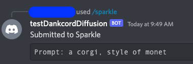
  4. Type in a prompt such as a corgi, style of monet.
    A response from YourBotName should appear with the response Submitted to Sparkle: YourPromptHere, as shown in Figure 4.

    First response from AWS Lambda function

    Figure 4. First response from AWS Lambda function

    It will take 10 minutes for an EC2 instance to start with an ECS Task running on the instance. Once an ECS Task is running on the instance, inference times should reduce to under 30 seconds, depending on the request.
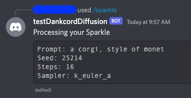
    When an ECS Task is running your request, you will see a Processing your Sparkle message, as shown in Figure 5.

    Amazon ECS task processing a request

    Figure 5. Amazon ECS task processing a request

    The message is complete when it says Completed your Sparkle! as shown in Figure 6.

    Amazon ECS task returning the final response

    Figure 6. Amazon ECS task returning the final response

Cleaning up

To avoid incurring future charges, delete the resources created by the Terraform script.

  1. Return to the directory where you deployed your terraform script.
  2. To destroy the infrastructure in AWS, run the command terraform destroy.
  3. When prompted to confirm that you want to destroy the infrastructure, type yes and press Enter.

Conclusion

In summary, we created a solution that allows members of a Discord server to create images from text with a Stable Diffusion model. With this implementation, the deployment can scale to many Discord Servers and handle over one hundred requests per second.

Create projects on AWS that lower the bar to entry for people wanting to try text to image models.

AWS CIRT announces the release of five publicly available workshops

Post Syndicated from Steve de Vera original https://aws.amazon.com/blogs/security/aws-cirt-announces-the-release-of-five-publicly-available-workshops/

Greetings from the AWS Customer Incident Response Team (CIRT)! AWS CIRT is dedicated to supporting customers during active security events on the customer side of the AWS Shared Responsibility Model.

Over the past year, AWS CIRT has responded to hundreds of such security events, including the unauthorized use of AWS Identity and Access Management (IAM) credentials, ransomware and data deletion in an AWS account, and billing increases due to the creation of unauthorized resources to mine cryptocurrency.

We are excited to release five workshops that simulate these security events to help you learn the tools and procedures that AWS CIRT uses on a daily basis to detect, investigate, and respond to such security events. The workshops cover AWS services and tools, such as Amazon GuardDuty, Amazon CloudTrail, Amazon CloudWatch, Amazon Athena, and AWS WAF, as well as some open source tools written and published by AWS CIRT.

To access the workshops, you just need an AWS account, an internet connection, and the desire to learn more about incident response in the AWS Cloud! Choose the following links to access the workshops.

Unauthorized IAM Credential Use – Security Event Simulation and Detection

During this workshop, you will simulate the unauthorized use of IAM credentials by using a script invoked within AWS CloudShell. The script will perform reconnaissance and privilege escalation activities that have been commonly seen by AWS CIRT and that are typically performed during similar events of this nature. You will also learn some tools and processes that AWS CIRT uses, and how to use these tools to find evidence of unauthorized activity by using IAM credentials.

Ransomware on S3 – Security Event Simulation and Detection

During this workshop, you will use an AWS CloudFormation template to replicate an environment with multiple IAM users and five Amazon Simple Storage Service (Amazon S3) buckets. AWS CloudShell will then run a bash script that simulates data exfiltration and data deletion events that replicate a ransomware-based security event. You will also learn the tools and processes that AWS CIRT uses to respond to similar events, and how to use these tools to find evidence of unauthorized S3 bucket and object deletions.

Cryptominer Based Security Events – Simulation and Detection

During this workshop, you will simulate a cryptomining security event by using a CloudFormation template to initialize three Amazon Elastic Compute Cloud (Amazon EC2) instances. These EC2 instances will mimic cryptomining activity by performing DNS requests to known cryptomining domains. You will also learn the tools and processes that AWS CIRT uses to respond to similar events, and how to use these tools to find evidence of unauthorized creation of EC2 instances and communication with known cryptomining domains.

SSRF on IMDSv1 – Simulation and Detection

During this workshop, you will simulate the unauthorized use of a web application that is hosted on an EC2 instance configured to use Instance Metadata Service Version 1 (IMDSv1) and vulnerable to server side request forgery (SSRF). You will learn how web application vulnerabilities, such as SSRF, can be used to obtain credentials from an EC2 instance. You will also learn the tools and processes that AWS CIRT uses to respond to this type of access, and how to use these tools to find evidence of the unauthorized use of EC2 instance credentials through web application vulnerabilities such as SSRF.

AWS CIRT Toolkit For Automating Incident Response Preparedness

During this workshop, you will install and experiment with some common tools and utilities that AWS CIRT uses on a daily basis to detect security misconfigurations, respond to active events, and assist customers with protecting their infrastructure.

If you have feedback about this post, submit comments in the Comments section below. If you have questions about this post, contact AWS Support.

Want more AWS Security news? Follow us on Twitter.

Author

Steve de Vera

Steve is the Incident Response Watch Lead for the US Pacific region of the AWS CIRT. He is passionate about American-style BBQ and is a certified competition BBQ judge. He has a dog named Brisket.

Enabling load-balancing of non-HTTP(s) traffic on AWS Wavelength

Post Syndicated from Sheila Busser original https://aws.amazon.com/blogs/compute/enabling-load-balancing-of-non-https-traffic-on-aws-wavelength/

This blog post is written by Jack Chen, Telco Solutions Architect, and Robert Belson, Developer Advocate.

AWS Wavelength embeds AWS compute and storage services within 5G networks, providing mobile edge computing infrastructure for developing, deploying, and scaling ultra-low-latency applications. AWS recently introduced support for Application Load Balancer (ALB) in AWS Wavelength zones. Although ALB addresses Layer-7 load balancing use cases, some low latency applications that get deployed in AWS Wavelength Zones rely on UDP-based protocols, such as QUIC, WebRTC, and SRT, which can’t be load-balanced by Layer-7 Load Balancers. In this post, we’ll review popular load-balancing patterns on AWS Wavelength, including a proposed architecture demonstrating how DNS-based load balancing can address customer requirements for load-balancing non-HTTP(s) traffic across multiple Amazon Elastic Compute Cloud (Amazon EC2) instances. This solution also builds a foundation for automatic scale-up and scale-down capabilities for workloads running in an AWS Wavelength Zone.

Load balancing use cases in AWS Wavelength

In the AWS Regions, customers looking to deploy highly-available edge applications often consider Amazon Elastic Load Balancing (Amazon ELB) as an approach to automatically distribute incoming application traffic across multiple targets in one or more Availability Zones (AZs). However, at the time of this publication, AWS-managed Network Load Balancer (NLB) isn’t supported in AWS Wavelength Zones and ALB is being rolled out to all AWS Wavelength Zones globally. As a result, this post will seek to document general architectural guidance for load balancing solutions on AWS Wavelength.

As one of the most prominent AWS Wavelength use cases, highly-immersive video streaming over UDP using protocols such as WebRTC at scale often require a load balancing solution to accommodate surges in traffic, either due to live events or general customer access patterns. These use cases, relying on Layer-4 traffic, can’t be load-balanced from a Layer-7 ALB. Instead, Layer-4 load balancing is needed.

To date, two infrastructure deployments involving Layer-4 load balancers are most often seen:

  • Amazon EC2-based deployments: Often the environment of choice for earlier-stage enterprises and ISVs, a fleet of EC2 instances will leverage a load balancer for high-throughput use cases, such as video streaming, data analytics, or Industrial IoT (IIoT) applications
  • Amazon EKS deployments: Customers looking to optimize performance and cost efficiency of their infrastructure can leverage containerized deployments at the edge to manage their AWS Wavelength Zone applications. In turn, external load balancers could be configured to point to exposed services via NodePort objects. Furthermore, a more popular choice might be to leverage the AWS Load Balancer Controller to provision an ALB when you create a Kubernetes Ingress.

Regardless of deployment type, the following design constraints must be considered:

  • Target registration: For load balancing solutions not managed by AWS, seamless solutions to load balancer target registration must be managed by the customer. As one potential solution, visit a recent HAProxyConf presentation, Practical Advice for Load Balancing at the Network Edge.
  • Edge Discovery: Although DNS records can be populated into Amazon Route 53 for each carrier-facing endpoint, DNS won’t deterministically route mobile clients to the most optimal mobile endpoint. When available, edge discovery services are required to most effectively route mobile clients to the lowest latency endpoint.
  • Cross-zone load balancing: Given the hub-and-spoke design of AWS Wavelength, customer-managed load balancers should proxy traffic only to that AWS Wavelength Zone.

Solution overview – Amazon EC2

In this solution, we’ll present a solution for a highly-available load balancing solution in a single AWS Wavelength Zone for an Amazon EC2-based deployment. In a separate post, we’ll cover the needed configurations for the AWS Load Balancer Controller in AWS Wavelength for Amazon Elastic Kubernetes Service (Amazon EKS) clusters.

The proposed solution introduces DNS-based load balancing, a technique to abstract away the complexity of intelligent load-balancing software and allow your Domain Name System (DNS) resolvers to distribute traffic (equally, or in a weighted distribution) to your set of endpoints.

Our solution leverages the weighted routing policy in Route 53 to resolve inbound DNS queries to multiple EC2 instances running within an AWS Wavelength zone. As EC2 instances for a given workload get deployed in an AWS Wavelength zone, Carrier IP addresses can be assigned to the network interfaces at launch.

Through this solution, Carrier IP addresses attached to AWS Wavelength instances are automatically added as DNS records for the customer-provided public hosted zone.

To determine how Route 53 responds to queries, given an arbitrary number of records of a public hosted zone, Route53 offers numerous routing policies:

Simple routing policy – In the event that you must route traffic to a single resource in an AWS Wavelength Zone, simple routing can be used. A single record can contain multiple IP addresses, but Route 53 returns the values in a random order to the client.

Weighted routing policy – To route traffic more deterministically using a set of proportions that you specify, this policy can be selected. For example, if you would like Carrier IP A to receive 50% of the traffic and Carrier IP B to receive 50% of the traffic, we’ll create two individual A records (one for each Carrier IP) with a weight of 50 and 50, respectively. Learn more about Route 53 routing policies by visiting the Route 53 Developer Guide.

The proposed solution leverages weighted routing policy in Route 53 DNS to route traffic to multiple EC2 instances running within an AWS Wavelength zone.

Reference architecture

The following diagram illustrates the load-balancing component of the solution, where EC2 instances in an AWS Wavelength zone are assigned Carrier IP addresses. A weighted DNS record for a host (e.g., www.example.com) is updated with Carrier IP addresses.

DNS-based load balancing

When a device makes a DNS query, it will be returned to one of the Carrier IP addresses associated with the given domain name. With a large number of devices, we expect a fair distribution of load across all EC2 instances in the resource pool. Given the highly ephemeral mobile edge environments, it’s likely that Carrier IPs could frequently be allocated to accommodate a workload and released shortly thereafter. However, this unpredictable behavior could yield stale DNS records, resulting in a “blackhole” – routes to endpoints that no longer exist.

Time-To-Live (TTL) is a DNS attribute that specifies the amount of time, in seconds, that you want DNS recursive resolvers to cache information about this record.

In our example, we should set to 30 seconds to force DNS resolvers to retrieve the latest records from the authoritative nameservers and minimize stale DNS responses. However, a lower TTL has a direct impact on cost, as a result of increased number of calls from recursive resolvers to Route53 to constantly retrieve the latest records.

The core components of the solution are as follows:

Alongside the services above in the AWS Wavelength Zone, the following services are also leveraged in the AWS Region:

  • AWS Lambda – a serverless event-driven function that makes API calls to the Route 53 service to update DNS records.
  • Amazon EventBridge– a serverless event bus that reacts to EC2 instance lifecycle events and invokes the Lambda function to make DNS updates.
  • Route 53– cloud DNS service with a domain record pointing to AWS Wavelength-hosted resources.

In this post, we intentionally leave the specific load balancing software solution up to the customer. Customers can leverage various popular load balancers available on the AWS Marketplace, such as HAProxy and NGINX. To focus our solution on the auto-registration of DNS records to create functional load balancing, this solution is designed to support stateless workloads only. To support stateful workloads, sticky sessions – a process in which routes requests to the same target in a target group – must be configured by the underlying load balancer solution and are outside of the scope of what DNS can provide natively.

Automation overview

Using the aforementioned components, we can implement the following workflow automation:

Event-driven Auto Scaling Workflow

Amazon CloudWatch alarm can trigger the Auto Scaling group Scale out or Scale in event by adding or removing EC2 instances. Eventbridge will detect the EC2 instance state change event and invoke the Lambda function. This function will update the DNS record in Route53 by either adding (scale out) or deleting (scale in) a weighted A record associated with the EC2 instance changing state.

Configuration of the automatic auto scaling policy is out of the scope of this post. There are many auto scaling triggers that you can consider using, based on predefined and custom metrics such as memory utilization. For the demo purposes, we will be leveraging manual auto scaling.

In addition to the core components that were already described, our solution also utilizes AWS Identity and Access Management (IAM) policies and CloudWatch. Both services are key components to building AWS Well-Architected solutions on AWS. We also use AWS Systems Manager Parameter Store to keep track of user input parameters. The deployment of the solution is automated via AWS CloudFormation templates. The Lambda function provided should be uploaded to an AWS Simple Storage Service (Amazon S3) bucket.

Amazon Virtual Private Cloud (Amazon VPC), subnets, Carrier Gateway, and Route Tables are foundational building blocks for AWS-based networking infrastructure. In our deployment, we are creating a new VPC, one subnet in an AWS Wavelength zone of your choice, a Carrier Gateway, and updating the route table for this subnet to point the default route to the Carrier Gateway.

Wavelength VPC architecture.

Deployment prerequisites

The following are prerequisites to deploy the described solution in your account:

  • Access to an AWS Wavelength zone. If your account is not allow-listed to use AWS Wavelength zones, then opt-in to AWS Wavelength zones here.
  • Public DNS Hosted Zone hosted in Route 53. You must have access to a registered public domain to deploy this solution. The zone for this domain should be hosted in the same account where you plan to deploy AWS Wavelength workloads.
    If you don’t have a public domain, then you can register a new one. Note that there will be a service charge for the domain registration.
  • Amazon S3 bucket. For the Lambda function that updates DNS records in Route 53, store the source code as a .zip file in an Amazon S3 bucket.
  • Amazon EC2 Key pair. You can use an existing Key pair for the deployment. If you don’t have a KeyPair in the region where you plan to deploy this solution, then create one by following these instructions.
  • 4G or 5G-connected device. Although the infrastructure can be deployed independent of the underlying connected devices, testing the connectivity will require a mobile device on one of the Wavelength partner’s networks. View the complete list of Telecommunications providers and Wavelength Zone locations to learn more.

Conclusion

In this post, we demonstrated how to implement DNS-based load balancing for workloads running in an AWS Wavelength zone. We deployed the solution that used the EventBridge Rule and the Lambda function to update DNS records hosted by Route53. If you want to learn more about AWS Wavelength, subscribe to AWS Compute Blog channel here.

Run fault tolerant and cost-optimized Spark clusters using Amazon EMR on EKS and Amazon EC2 Spot Instances

Post Syndicated from Kinnar Kumar Sen original https://aws.amazon.com/blogs/big-data/run-fault-tolerant-and-cost-optimized-spark-clusters-using-amazon-emr-on-eks-and-amazon-ec2-spot-instances/

Amazon EMR on EKS is a deployment option in Amazon EMR that allows you to run Spark jobs on Amazon Elastic Kubernetes Service (Amazon EKS). Amazon Elastic Compute Cloud (Amazon EC2) Spot Instances save you up to 90% over On-Demand Instances, and is a great way to cost optimize the Spark workloads running on Amazon EMR on EKS. Because Spot is an interruptible service, if we can move or reuse the intermediate shuffle files, it improves the overall stability and SLA of the job. The latest versions of Amazon EMR on EKS have integrated Spark features to enable this capability.

In this post, we discuss these features—Node Decommissioning and Persistent Volume Claim (PVC) reuse—and their impact on increasing the fault tolerance of Spark jobs on Amazon EMR on EKS when cost optimizing using EC2 Spot Instances.

Amazon EMR on EKS and Spot

EC2 Spot Instances are spare EC2 capacity provided at a steep discount of up to 90% over On-Demand prices. Spot Instances are a great choice for stateless and flexible workloads. The caveat with this discount and spare capacity is that Amazon EC2 can interrupt an instance with a proactive or reactive (2-minute) warning when it needs the capacity back. You can provision compute capacity in an EKS cluster using Spot Instances using a managed or self-managed node group and provide cost optimization for your workloads.

Amazon EMR on EKS uses Amazon EKS to run jobs with the EMR runtime for Apache Spark, which can be cost optimized by running the Spark executors on Spot. It provides up to 61% lower costs and up to 68% performance improvement for Spark workloads on Amazon EKS. The Spark application launches a driver and executors to run the computation. Spark is a semi-fault tolerant framework that is resilient to executor loss due to an interruption and therefore can run on EC2 Spot. On the other hand, when the driver is interrupted, the job fails. Hence, we recommend running drivers on on-demand instances. Some of the best practices for running Spark on Amazon EKS are applicable with Amazon EMR on EKS.

EC2 Spot instances also helps in cost optimization by improving the overall throughput of the job. This can be achieved by auto-scaling the cluster using Cluster Autoscaler (for managed nodegroups) or Karpenter.

Though Spark executors are resilient to Spot interruptions, the shuffle files and RDD data is lost when the executor gets killed. The lost shuffle files need to be recomputed, which increases the overall runtime of the job. Apache Spark has released two features (in versions 3.1 and 3.2) that addresses this issue. Amazon EMR on EKS released features such as node decommissioning (version 6.3) and PVC reuse (version 6.8) to simplify recovery and reuse shuffle files, which increases the overall resiliency of your application.

Node decommissioning

The node decommissioning feature works by preventing scheduling of new jobs on the nodes that are to be decommissioned. It also moves any shuffle files or cache present in those nodes to other executors (peers). If there are no other available executors, the shuffle files and cache are moved to a remote fallback storage.

Node Decommissioning

Fig 1 : Node Decommissioning

Let’s look at the decommission steps in more detail.

If one of the nodes that is running executors is interrupted, the executor starts the process of decommissioning and sends the message to the driver:

21/05/05 17:41:41 WARN KubernetesClusterSchedulerBackend$KubernetesDriverEndpoint: Received executor 7 decommissioned message
21/05/05 17:41:41 DEBUG TaskSetManager: Valid locality levels for TaskSet 2.0: NO_PREF, ANY
21/05/05 17:41:41 INFO KubernetesClusterSchedulerBackend: Decommission executors: 7
21/05/05 17:41:41 DEBUG TaskSchedulerImpl: parentName: , name: TaskSet_2.0, runningTasks: 10
21/05/05 17:41:41 INFO BlockManagerMasterEndpoint: Mark BlockManagers (BlockManagerId(7, 192.168.82.107, 39007, None)) as being decommissioning.
21/05/05 20:22:17 INFO CoarseGrainedExecutorBackend: Decommission executor 1.
21/05/05 20:22:17 INFO CoarseGrainedExecutorBackend: Will exit when finished decommissioning
21/05/05 20:22:17 INFO BlockManager: Starting block manager decommissioning process...
21/05/05 20:22:17 DEBUG FileSystem: Looking for FS supporting s3a

The executor looks for RDD or shuffle files and tries to replicate or migrate those files. It first tries to find a peer executor. If successful, it will move the files to the peer executor:

22/06/07 20:41:38 INFO ShuffleStatus: Updating map output for 46 to BlockManagerId(4, 192.168.13.235, 34737, None)
22/06/07 20:41:38 DEBUG BlockManagerMasterEndpoint: Received shuffle data block update for 0 46, ignore.
22/06/07 20:41:38 DEBUG BlockManagerMasterEndpoint: Received shuffle index block update for 0 46, updating.

However, if It is not able to find a peer executor, it will try to move the files to a fallback storage if available.

Fallback Storage

Fig 2: Fallback Storage

The executor is then decommissioned. When a new executor comes up, the shuffle files are reused:

22/06/07 20:42:50 INFO BasicExecutorFeatureStep: Adding decommission script to lifecycle
22/06/07 20:42:50 DEBUG ExecutorPodsAllocator: Requested executor with id 19 from Kubernetes.
22/06/07 20:42:50 DEBUG ExecutorPodsWatchSnapshotSource: Received executor pod update for pod named amazon-reviews-word-count-bfd0a5813fd1b80f-exec-19, action ADDED
22/06/07 20:42:50 DEBUG BlockManagerMasterEndpoint: Received shuffle index block update for 0 52, updating.
22/06/07 20:42:50 INFO ShuffleStatus: Recover 52 BlockManagerId(fallback, remote, 7337, None)

The key advantage of this process is that it enables migrates blocks and shuffle data, thereby reducing recomputation, which adds to the overall resiliency of the system and reduces runtime. This process can be triggered by a Spot interruption signal (Sigterm) and node draining. Node draining  may happen due to high-priority task scheduling or independently.

When you use Amazon EMR on EKS with managed node groups/Karpenter, the Spot interruption handling is automated, wherein Amazon EKS gracefully drains and rebalances the Spot nodes to minimize application disruption when a Spot node is at elevated risk of interruption. If you’re using managed node groups/Karpenter, the decommission gets triggered when the nodes are getting drained and because it’s proactive, it gives you more time (at least 2 minutes) to move the files. In the case of self-managed node groups, we recommend installing the AWS Node Termination Handler to handle the interruption, and the decommission is triggered when the reactive (2-minute) notification is received. We recommend to use Karpenter with Spot Instances as it has faster node scheduling with early pod binding and binpacking to optimize the resource utilization.

The following code enables this configuration; more details are available on GitHub:

"spark.decommission.enabled": "true"
"spark.storage.decommission.rddBlocks.enabled": "true"
"spark.storage.decommission.shuffleBlocks.enabled" : "true"
"spark.storage.decommission.enabled": "true"
"spark.storage.decommission.fallbackStorage.path": "s3://<<bucket>>"

PVC reuse

Apache Spark enabled dynamic PVC in version 3.1, which is useful with dynamic allocation because we don’t have to pre-create the claims or volumes for the executors and delete them after completion. PVC enables true decoupling of data and processing when we’re running Spark jobs on Kubernetes, because we can use it as a local storage to spill in-process files too. The latest version of Amazon EMR 6.8 has integrated the PVC reuse feature of Spark, wherein if an executor is terminated due to EC2 Spot interruption or any other reason (JVM), then the PVC is not deleted but persisted and reattached to another executor. If there are shuffle files in that volume, then they are reused.

As with node decommission, this reduces the overall runtime because we don’t have to recompute the shuffle files. We also save the time required to request a new volume for an executor, and shuffle files can be reused without moving the files round.

The following diagram illustrates this workflow.

PVC Reuse

Fig 3: PVC Reuse

Let’s look at the steps in more detail.

If one or more of the nodes that are running executors is interrupted, the underlying pods get terminated and the driver gets the update. Note that the driver is the owner of the PVC of the executors, and they are not terminated. See the following code:

22/06/15 23:25:07 DEBUG ExecutorPodsWatchSnapshotSource: Received executor pod update for pod named amazon-reviews-word-count-9ee82b8169a75183-exec-3, action DELETED
22/06/15 23:25:07 DEBUG ExecutorPodsWatchSnapshotSource: Received executor pod update for pod named amazon-reviews-word-count-9ee82b8169a75183-exec-6, action MODIFIED
22/06/15 23:25:07 DEBUG ExecutorPodsWatchSnapshotSource: Received executor pod update for pod named amazon-reviews-word-count-9ee82b8169a75183-exec-6, action DELETED
22/06/15 23:25:07 DEBUG ExecutorPodsWatchSnapshotSource: Received executor pod update for pod named amazon-reviews-word-count-9ee82b8169a75183-exec-3, action MODIFIED

The ExecutorPodsAllocator tries to allocate new executor pods to replace the ones terminated due to interruption. During the allocation, it figures out how many of the existing PVCs have files and can be reused:

22/06/15 23:25:23 INFO ExecutorPodsAllocator: Found 2 reusable PVCs from 10 PVCs

The ExecutorPodsAllocator requests for a pod and when it launches it, the PVC is reused. In the following example, the PVC from executor 6 is reused for new executor pod 11:

22/06/15 23:25:23 DEBUG ExecutorPodsAllocator: Requested executor with id 11 from Kubernetes.
22/06/15 23:25:24 DEBUG ExecutorPodsWatchSnapshotSource: Received executor pod update for pod named amazon-reviews-word-count-9ee82b8169a75183-exec-11, action ADDED
22/06/15 23:25:24 INFO KubernetesClientUtils: Spark configuration files loaded from Some(/usr/lib/spark/conf) : log4j.properties,spark-env.sh,hive-site.xml,metrics.properties
22/06/15 23:25:24 INFO BasicExecutorFeatureStep: Decommissioning not enabled, skipping shutdown script
22/06/15 23:25:24 DEBUG ExecutorPodsWatchSnapshotSource: Received executor pod update for pod named amazon-reviews-word-count-9ee82b8169a75183-exec-11, action MODIFIED
22/06/15 23:25:24 INFO ExecutorPodsAllocator: Reuse PersistentVolumeClaim amazon-reviews-word-count-9ee82b8169a75183-exec-6-pvc-0

The shuffle files, if present in the PVC are reused.

The key advantage of this technique is that it allows us to reuse pre-computed shuffle files in their original location, thereby reducing the time of the overall job run.

This works for both static and dynamic PVCs. Amazon EKS offers three different storage offerings, which can be encrypted too: Amazon Elastic Block Store (Amazon EBS), Amazon Elastic File System (Amazon EFS), and Amazon FSx for Lustre. We recommend using dynamic PVCs with Amazon EBS because with static PVCs, you would need to create multiple PVCs.

The following code enables this configuration; more details are available on GitHub:

"spark.kubernetes.driver.ownPersistentVolumeClaim": "true"
"spark.kubernetes.driver.reusePersistentVolumeClaim": "true"

For this to work, we need to enable PVC with Amazon EKS and mention the details in the Spark runtime configuration. For instructions, refer to How do I use persistent storage in Amazon EKS? The following code contains the Spark configuration details for using PVC as local storage; other details are available on GitHub:

"spark.kubernetes.executor.volumes.persistentVolumeClaim.spark-local-dir-1.mount.readOnly": "false"
"spark.kubernetes.executor.volumes.persistentVolumeClaim.spark-local-dir-1.options.claimName": "OnDemand"
"spark.kubernetes.executor.volumes.persistentVolumeClaim.spark-local-dir-1.options.storageClass": "spark-sc"
"spark.kubernetes.executor.volumes.persistentVolumeClaim.spark-local-dir-1.options.sizeLimit": "10Gi"
"spark.kubernetes.executor.volumes.persistentVolumeClaim.spark-local-dir-1.mount.path": "/var/data/spill"

Conclusion

With Amazon EMR on EKS (6.9) and the features discussed in this post, you can further reduce the overall runtime for Spark jobs when running with Spot Instances. This also improves the overall resiliency and flexibility of the job while cost optimizing the workload on EC2 Spot.

Try out the EMR on EKS workshop for improved performance when running Spark workloads on Kubernetes and cost optimize using EC2 Spot Instances.


About the Author

Kinnar Kumar Sen is a Sr. Solutions Architect at Amazon Web Services (AWS) focusing on Flexible Compute. As a part of the EC2 Flexible Compute team, he works with customers to guide them to the most elastic and efficient compute options that are suitable for their workload running on AWS. Kinnar has more than 15 years of industry experience working in research, consultancy, engineering, and architecture.

Introducing the Security Design of the AWS Nitro System whitepaper

Post Syndicated from J.D. Bean original https://aws.amazon.com/blogs/security/introducing-the-security-design-of-the-aws-nitro-system-whitepaper/

AWS recently released a whitepaper on the Security Design of the AWS Nitro System. The Nitro System is a combination of purpose-built server designs, data processors, system management components, and specialized firmware that serves as the underlying virtualization technology that powers all Amazon Elastic Compute Cloud (Amazon EC2) instances launched since early 2018. With the Nitro System, AWS undertook an effort to reimagine the architecture of virtualization to deliver security, isolation, performance, cost savings, and a pace of innovation that our customers require.

This whitepaper is a detailed design document on the inner workings of the AWS Nitro System, and how we use it to help secure your most critical workloads. This is the first time that AWS has provided such a detailed design document on the Nitro System and how it offers a no-operator access design and strong tenant isolation. The whitepaper describes the security design of the Nitro System in detail to help you evaluate Amazon EC2 for your sensitive workloads.

Three key components of the Nitro System are used to implement this design:

  • Purpose-built Nitro Cards – Hardware devices designed by AWS that provide overall system control and I/O virtualization that is independent of the main system board with its CPUs and memory.
  • Nitro Security Chip – Enables a secure boot process for the overall system based on a hardware root of trust, the ability to offer bare metal instances, and defense-in-depth that offers protection to the server from unauthorized modification of system firmware.
  • Nitro Hypervisor – A deliberately minimized and firmware-like hypervisor designed to provide strong resource isolation, and performance that is nearly indistinguishable from a bare metal server.

The whitepaper describes the fundamental architectural change introduced by the Nitro System compared to previous approaches to virtualization. It discusses the three key components of the Nitro System, and provides a demonstration of how these components work together by walking through what happens when a new Amazon Elastic Block Store (Amazon EBS) volume is added to a running EC2 instance. The whitepaper also discusses how the Nitro System is designed to eliminate the possibility of administrator access to an EC2 server, the overall passive communications design of the Nitro System, and the Nitro System change management process. Finally, the paper surveys important aspects of the EC2 system design that provide mitigations against potential side-channel issues that can arise in compute environments.

The whitepaper dives deep into each of these considerations, offering a detailed picture of the Nitro System security design. For more information about cloud security at AWS, contact us.

If you have feedback about this post, submit comments in the Comments section below. If you have questions about this post, contact AWS Support.

Want more AWS Security news? Follow us on Twitter.

J.D. Bean

J.D. is a Principal Security Architect for Amazon EC2 based out of New York City. His interests include security, privacy, and compliance. He is passionate about his work enabling AWS customers’ successful cloud journeys. J.D. holds a Bachelor of Arts from The George Washington University and a Juris Doctor from New York University School of Law.

AWS Week in Review – December 19, 2022

Post Syndicated from Sébastien Stormacq original https://aws.amazon.com/blogs/aws/aws-week-in-review-december-19-2022/

We are half way between the re:Invent conference and the end-of-year holidays, and I did expect the cadence of releases and news to slow down a bit, but nothing is further away from reality. Our teams continue to listen to your feedback and release new capabilities and incremental improvements.

This week, many items caught my attention. Here is my summary.

The AWS Pricing Calculator for Amazon EC2 is getting a redesign to provide you with a simplified, consistent, and efficient calculator to estimate costs. It also added a way to bulk estimate costs for EC2 instances, EC2 Dedicated Hosts, and Amazon EBS services. Try it for yourself today.

AWS Pricing Calculator

Amazon CloudWatch Metrics Insights alarms now enables you to trigger alarms on entire fleets of dynamically changing resources (such as automatically scaling EC2 instances) with a single alarm using standard SQL queries. For example, you can now write a query like this to collect data about CPU utilization over your entire dynamic fleet of EC2 instances.

SELECT AVG(CPUUtilization) FROM SCHEMA("AWS/EC2", InstanceId)

AWS Amplify is a command line tool and a set of libraries to help you to build web and mobile applications connected to a cloud backend. We released Amplify Library for Android 2.0, with improvements and simplifications for user authentication. The team also released Amplify JavaScript library version 5, with improvements for React and React Native developers, such as a new notifications channel, also known as in-app messaging, that developers can use to display contextual messages to their users based on their behavior. The Amplify JavaScript library has also received improvements to reduce the overall bundle size and installation size.

Amazon Connect added granular access control based on resource tags for routing profiles, security profiles, users, and queues. It also adds bulk import for user hierarchy tags. This allows you to use attribute-based access control policies for Amazon Connect resources.

Amazon RDS Proxy now supports PostgreSQL major version 14. RDS Proxy is a fully managed, highly available database proxy for Amazon Relational Database Service (Amazon RDS) that makes applications more scalable, more resilient to database failures, and more secure. It is typically used by serverless applications that can have a large number of open connections to the database server and may open and close database connections at a high rate, exhausting database memory and compute resources.

AWS Gateway Load Balancer endpoints now support Ipv6 addresses. You can now send IPv6 traffic through Gateway Load Balancers and its endpoints to distribute traffic flows to dual stack appliance targets.

Amazon Location Service now provides Open Data Maps maps, in addition to ESRI and Here maps. I also noticed that Amazon is a core member of the new Overture Maps Foundation, officially hosted by the Linux Foundation. The mission of the Overture Maps Foundation is to power new map products through openly available datasets that can be used and reused across applications and businesses. The program is driven by Amazon Web Services (AWS), Facebook’s parent company Meta, Microsoft, and Dutch mapping company TomTom.

AWS Mainframe Modernization is a set of managed tools providing infrastructure and software for migrating, modernizing, and running mainframe applications. It is now available in three additional AWS Regions and supports AWS CloudFormation, AWS PrivateLink, AWS Key Management Service.

X in Y. Jeff started this section a while ago to list the expansion of new services and capabilities to additional Regions. I noticed 11 Regional expansions this week:

Other AWS News
This week, I also noticed these AWS news items:

Amazon SageMaker turned 5 years old 🎉🎂. You can read the initial blog post we published at the time. To celebrate the event, the Amazon Science published this article where AWS’s Vice President Bratin Saha reflects on the past and future of AWS’s machine learning tools and AI services.

The security blog published a great post about the Cedar policy language. It explains how Amazon Verified Permissions provides a pre-built, flexible permissions system that you can use to build permissions based on both ABAC and RBAC in your applications. Cedar policy language is also at the heart of Amazon Verified Access I blogged about during re:Invent.

And just like every week, my most excellent colleague Ricardo published the open source newsletter.

Upcoming AWS Events
Check your calendars and sign up for these AWS events:

AWS re:Invent recaps in your area. During the re:Invent week, we had lots of new announcements, and in the next weeks, you can find in your area a recap of all these launches. All the events will be posted on this site, so check it regularly to find an event nearby.

AWS re:Invent keynotes, leadership sessions, and breakout sessions are available on demand. I recommend that you check the playlists and find the talks about your favorite topics in one collection.

AWS Summits season will restart in Q2 2023. The dates and locations will be announced here.

Stay Informed
That is my selection for this week! Heads up – the Week in Review will be taking a short break for the end of the year, but we’ll be back with regular updates starting on January 9, 2023. To better keep up with all of this news, do not forget to check out the following resources:

— seb
This post is part of our Week in Review series. Check back each week for a quick roundup of interesting news and announcements from AWS!

Genomics workflows, Part 2: simplify Snakemake launches

Post Syndicated from Rostislav Markov original https://aws.amazon.com/blogs/architecture/genomics-workflows-part-2-simplify-snakemake-launches/

Genomics workflows are high-performance computing workloads. In Part 1 of this series, we demonstrated how life-science research teams can focus on scientific discovery without the associated heavy lifting. We used regenie for large genome-wide association studies. Our design pattern built on AWS Step Functions with AWS Batch and Amazon FSx for Lustre.

In Part 2, we explore genomics workloads with built-in workflow logic. Historically, running bioinformatics data pipelines was a manual and error-prone task. Over the last years, multiple workflow management systems have emerged. An example of these is the Snakemake workflow management system with Tibanna orchestration. We discuss the solution design and how you can fully automate the launch with Amazon Web Services (AWS).

Use case

We focus on the use case of Snakemake, an open-source utility for whole genome sequence mapping in directed acyclic graph (DAG) format. Snakemake uses Snakefiles to declare workflow steps and commands. A Snakefile extends Python syntax to declare workflow steps such as mapping data sets to DAG structure and identifying variants. Consult the Snakemake tutorial for further information on workflow rules.

Snakefiles provide an exception from the general design pattern and an alternative to granular modeling workflow logic in Amazon States Language. In our real-life use case, we used Tibanna to orchestrate Snakemake. Tibanna is an open-source, AWS-native software that runs bioinformatics data pipelines. It supports Snakefile syntax, plus other workflow languages, including Common Workflow Language and Workflow Description Language (WDL).

We recommend using Amazon Genomics CLI, if Tibanna is not needed for your use case, and Amazon Omics, if your workflow definitions are compliant with the supported WDL and Nextflow specifications.

Solution overview

Snakemake is available as Docker image on GitHub. We push the image to Amazon Elastic Container Registry. Tibanna is also available as Docker image on GitHub—it comes with Snakemake. Consult the Tibanna installation guide for more information.

We store Snakefiles on Amazon Simple Storage Service (Amazon S3). We configure S3 Event Notifications on PUT request operations. The event notification triggers an AWS Lambda function. The Lambda function launches an AWS Fargate task, which overrides the task definition command with the appropriate Snakemake start command and arguments.

The launched AWS Fargate task pulls the Snakefiles at launch time for each job and prepares the Snakemake initiation commands. Once the Snakefiles are downloaded on the Fargate task, the Snakemake head initiation command is invoked to begin launching jobs using Tibanna. Tibanna invokes a Step Functions state machine which orchestrates the launch of Snakemake on Amazon Elastic Compute Cloud (Amazon EC2).

Amazon CloudWatch provides a consolidated overview of performance metrics, including elapsed time, failed jobs, and error types. You can keep logs of your failed jobs in CloudWatch Logs (Figure 1). You can set up filters to match specific error types, plus create subscriptions to deliver a real-time stream of your log events to Amazon Kinesis or Lambda for further retry.

Solution architecture for Snakemake with Tibanna on AWS

Figure 1. Solution architecture for Snakemake with Tibanna on AWS

Implementation considerations

Here, we describe some of the implementation considerations.

Creating Snakefiles

The launching point for the initiation depends on a Snakefile. Each Snakefile may contain one or more samples to be launched. The sheet resides in an S3 bucket. This adds flexibility and the ability to purge any sensitive or restrictive information after the job has been processed.

Invoking Tibanna

In order to launch Snakemake DAGs using Tibanna, we will need to set up a new Tibanna Unicorn. A Tibanna Unicorn is an Step Functions state machine and a corresponding Lambda function for provisioning EC2 instances.

The state machine runs the following sequence:

  1. Create EC2 instance
  2. Check EC2 status
  3. Exit

After the Tibanna Unicorn has been created, we can start a Snakemake DAG using the following sample commands inside of the Fargate task.

$ export TIBANNA_DEFAULT_STEP_FUNCTION_NAME=YOUR_UNICORN_PROJECT
$ snakemake --tibanna --tibanna-config spot_instance=true --default-remote-prefix=YOUR_S3_BUCKET/BUCKET_PREFIX --retries 3.

The Snakemake command is used with the --tibanna flag to send launch requests to the Step Functions state machine in order to provision EC2 instances and run DAG tasks.

We recommend deploying the solution with AWS Serverless Application Model or the AWS Cloud Development Kit, both of which launch AWS CloudFormation.

Logging and troubleshooting

With this solution, each launch will automatically capture and retain start logs in a centralized location in Amazon CloudWatch Logs for tracing and auditing.

If there are issues during the launch of the Tibanna Step Function state machine, such as Amazon EC2 capacity limits, logs will be available in the S3 bucket that was specified during the Tibanna Unicorn creation process. There will be a file available in the format of <EXECUTION_ID>.log inside of the S3 bucket. This information is easily accessible via the command line interface. Use the following command to display specific log results or error messages.

tibanna log -j <EXECUTION_ID> -T 

Retries and EC2 Spot Instances

We advise to use Amazon EC2 Spot Instances, if possible, for additional cost savings. This option is available in the --tibanna-config arguments with the setting spot_instance=true.

This is optional, and you need to create retry logic in the event a Spot Instance gets reclaimed. You can include --retries=3 in your Tibanna launch command. This would ensure all rules are retried three times. You can also specify the number of retries for individual rules when defining the Snakemake DAG definition; for example:

rule a:
    output:
        "test.txt"
    retries: 3
    shell:
        "curl https://some.unreliable.server/test.txt > {output}"

If EC2 Spot Instance capacity is hit, you can automatically switch to using EC2 On-Demand Instances instead. Add the behavior_on_capacity_limit argument and set retry_without_spot=true.

Adding services

The presented solution can be adapted to use other compute services supported by Snakemake. These include Amazon Elastic Kubernetes Service and AWS ParallelCluster with Slurm Workload Manager plus Amazon FSx for Lustre volumes attached to the head node and cluster nodes.

To initiate jobs on ParallelCluster, install the AWS Systems Manager agent on the head node. This is the launching point into the cluster and used for submitting jobs to the initiation queue. Systems Manager is a secure way to remotely invoke commands on an EC2 instance without the need for SSH access. You can restrict access to your EC2 instance through IAM policies.

Conclusion

In this blog post, we demonstrated how life-science research teams can simplify the launch of Snakemake using AWS. We used Snakefiles and Tibanna to orchestrate workflow steps. Snakefiles provide an exception from the general design pattern and an alternative to Amazon States Language. File uploads to Amazon S3 served as our launching point for workflow initiations.

Stay tuned for Part 3 of this series, in which we create a job manager that administrates multiple workflows.

Related information

Amazon EMR launches support for Amazon EC2 C6i, M6i, I4i, R6i and R6id instances to improve cost performance for Spark workloads by 6–33%

Post Syndicated from Al MS original https://aws.amazon.com/blogs/big-data/amazon-emr-launches-support-for-amazon-ec2-c6i-m6i-i4i-r6i-and-r6id-instances-to-improve-cost-performance-for-spark-workloads-by-6-33/

Amazon EMR provides a managed service to easily run analytics applications using open-source frameworks such as Apache Spark, Hive, Presto, Trino, HBase, and Flink. The Amazon EMR runtime for Spark and Presto includes optimizations that provide over two times performance improvements over open-source Apache Spark and Presto, so that your applications run faster and at lower cost.

With Amazon EMR release 6.8, you can now use Amazon Elastic Compute Cloud (Amazon EC2) instances such as C6i, M6i, I4i, R6i, and R6id, which use the third-generation Intel Xeon scalable processors. Using these new instances with Amazon EMR improves cost-performance by an additional 5–33% over previous generation instances.

In this post, we describe how we estimated the cost-performance benefit from using Amazon EMR with these new instances compared to using equivalent previous generation instances.

Amazon EMR runtime performance improvements with EC2 I4i instances

We ran TPC-DS 3 TB benchmark queries on Amazon EMR 6.8 using the Amazon EMR runtime for Apache Spark (compatible with Apache Spark 3.3) with five node clusters of I4i instances with data in Amazon Simple Storage Service (Amazon S3), and compared it to equivalent sized I3 instances. We measured performance improvements using the total query runtime and geometric mean of query runtime across the TPC-DS 3 TB benchmark queries.

Our results showed between 36.41–44.39% improvement in total query runtime performance on I4i instance EMR clusters compared to equivalent I3 instance EMR clusters, and between 36–45.2% improvement in geometric mean. To measure cost improvement, we added up the Amazon EMR and Amazon EC2 cost per instance per hour (on-demand) and multiplied it by the total query runtime. Note that I4i 32XL instances were not benchmarked because I3 instances don’t have the 32 XL size available. We observed between 22.56–33.1% reduced instance hour cost on I4i instance EMR clusters compared to equivalent I3 instance EMR clusters to run the TPC-DS benchmark queries. All TPC-DS queries ran faster on I4i instance clusters compared to I3 instance clusters.

The following table shows the results from running TPC-DS 3 TB benchmark queries using Amazon EMR 6.8 over equivalent I3 and I4i instance EMR clusters.

Instance Size 16 XL 8 XL 4 XL 2 XL XL
Number of core instances in EMR cluster 5 5 5 5 5
Total query runtime on I3 (seconds) 4752.15457 4506.43694 7110.03042 11853.40336 21333.05743
Total query runtime on I4I (seconds) 2642.77407 2812.05517 4415.0023 7537.52779 12981.20251
Total query runtime improvement with I4I 44.39% 37.60% 37.90% 36.41% 39.15%
Geometric mean query runtime on I3 (sec) 34.99551 29.14821 41.53093 60.8069 95.46128
Geometric mean query runtime on I4I (sec) 19.17906 18.65311 25.66263 38.13503 56.95073
Geometric mean query runtime improvement with I4I 45.20% 36.01% 38.21% 37.29% 40.34%
EC2 I3 instance price ($ per hour) $4.990 $2.496 $1.248 $0.624 $0.312
EMR I3 instance price ($ per hour) $0.270 $0.270 $0.270 $0.156 $0.078
(EC2 + EMR) I3 instance price ($ per hour) $5.260 $2.766 $1.518 $0.780 $0.390
Cost of running on I3 ($ per instance) $6.943 $3.462 $2.998 $2.568 $2.311
EC2 I4I instance price ($ per hour) $5.491 $2.746 $1.373 $0.686 $0.343
EMR I4I price ($ per hour per instance) $1.373 $0.687 $0.343 $0.172 $0.086
(EC2 + EMR) I4I instance price ($ per hour) $6.864 $3.433 $1.716 $0.858 $0.429
Cost of running on I4I ($ per instance) $5.039 $2.681 $2.105 $1.795 $1.546
Total cost reduction with I4I including performance improvement -27.43% -22.56% -29.79% -30.09% -33.10%

The following graph shows per query improvements we observed on I4i 2XL instances with EMR Runtime for Spark on Amazon EMR version 6.8 compared to equivalent I3 2XL instances for the TPC-DS 3 TB benchmark.

Amazon EMR runtime performance improvements with EC2 M6i instances

M6i instances showed a similar performance improvement while running Apache Spark workloads compared to equivalent M5 instances. Our test results showed between 13.45–29.52% improvement in total query runtime for seven different instance sizes within the instance family, and between 7.98–25.37% improvement in geometric mean. On cost comparison, we observed 7.98–25.37% reduced instance hour cost on M6i instance EMR clusters compared to M5 EMR instance clusters to run the TPC-DS benchmark queries.

The following table shows the results from running TPC-DS 3 TB benchmark queries using Amazon EMR 6.8 over equivalent M6i and M5 instance EMR clusters.

Instance Size 24 XL 16 XL 12 XL 8 XL 4 XL 2 XL XL
Number of core instances in EMR cluster 5 5 5 5 5 5 5
Total query runtime on M5 (seconds) 4027.58043 3782.10766 3348.05362 3516.4308 5621.22532 10075.45109 17278.15146
Total query runtime on M6I (seconds) 3106.43834 2665.70607 2714.69862 3043.5975 4195.02715 8226.88301 14515.50394
Total query runtime improvement with M6I 22.87% 29.52% 18.92% 13.45% 25.37% 18.35% 15.99%
Geometric mean query runtime M5 (sec) 30.45437 28.5207 23.95314 23.55958 32.95975 49.43178 75.95984
Geometric mean query runtime M6I (sec) 23.76853 19.21783 19.16869 19.9574 24.23012 39.09965 60.79494
Geometric mean query runtime improvement with M6I 21.95% 32.62% 19.97% 15.29% 26.49% 20.90% 19.96%
EC2 M5 instance price ($ per hour) $4.61 $3.07 $2.30 $1.54 $0.77 $0.38 $0.19
EMR M5 instance price ($ per hour) $0.27 $0.27 $0.27 $0.27 $0.19 $0.10 $0.05
(EC2 + EMR) M5 instance price ($ per hour) $4.88 $3.34 $2.57 $1.81 $0.96 $0.48 $0.24
Cost of running on M5 ($ per instance) $5.46 $3.51 $2.39 $1.76 $1.50 $1.34 $1.15
EC2 M6I instance price ($ per hour) $4.61 $3.07 $2.30 $1.54 $0.77 $0.38 $0.19
EMR M6I price ($ per hour per instance) $1.15 $0.77 $0.58 $0.38 $0.19 $0.10 $0.05
(EC2 + EMR) M6I instance price ($ per hour) $5.76 $3.84 $2.88 $1.92 $0.96 $0.48 $0.24
Cost of running on M6I ($ per instance) $4.97 $2.84 $2.17 $1.62 $1.12 $1.10 $0.97
Total cost reduction with M6I including performance improvement -8.92% -19.02% -9.28% -7.98% -25.37% -18.35% -15.99%

Amazon EMR runtime performance improvements with EC2 R6i instances

R6i instances showed a similar performance improvement while running Apache Spark workloads compared to equivalent R5 instances. Our test results showed between 14.25–32.23% improvement in total query runtime for six different instance sizes within the instance family, and between 16.12–36.5% improvement in geometric mean. R5.xlarge instances didn’t have sufficient memory to run TPC-DS benchmark queries, and weren’t included in this comparison. On cost comparison, we observed 5.48–23.5% reduced instance hour cost on R6i instance EMR clusters compared to R5 EMR instance clusters to run the TPC-DS benchmark queries.

The following table shows the results from running TPC-DS 3 TB benchmark queries using Amazon EMR 6.8 over equivalent R6i and R5 instance EMR clusters.

Instance Size 24 XL 16 XL 12 XL 8 XL 4 XL 2XL
Number of core instances in EMR cluster 5 5 5 5 5 5
Total query runtime on R5 (seconds) 4024.4737 3715.74432 3552.97298 3535.69879 5379.73168 9121.41532
Total query runtime on R6I (seconds) 2865.83169 2518.24192 2513.4849 3031.71973 4544.44854 6977.9508
Total query runtime improvement with R6I 28.79% 32.23% 29.26% 14.25% 15.53% 23.50%
Geometric mean query runtime R5 (sec) 30.59066 28.30849 25.30903 23.85511 32.33391 47.28424
Geometric mean query runtime R6I (sec) 21.87897 17.97587 17.54117 20.00918 26.6277 34.52817
Geometric mean query runtime improvement with R6I 28.48% 36.50% 30.69% 16.12% 17.65% 26.98%
EC2 R5 instance price ($ per hour) $6.0480 $4.0320 $3.0240 $2.0160 $1.0080 $0.5040
EMR R5 instance price ($ per hour) $0.2700 $0.2700 $0.2700 $0.2700 $0.2520 $0.1260
(EC2 + EMR) R5 instance price ($ per hour) $6.3180 $4.3020 $3.2940 $2.2860 $1.2600 $0.6300
Cost of running on R5 ($ per instance) $7.0630 $4.4403 $3.2510 $2.2452 $1.8829 $1.5962
EC2 R6I instance price ($ per hour) $6.0480 $4.0320 $3.0240 $2.0160 $1.0080 $0.5040
EMR R6I price ($ per hour per instance) $1.5120 $1.0080 $0.7560 $0.5040 $0.2520 $0.1260
(EC2 + EMR) R6I instance price ($ per hour) $7.5600 $5.0400 $3.7800 $2.5200 $1.2600 $0.6300
Cost of running on R6I ($ per instance) $6.0182 $3.5255 $2.6392 $2.1222 $1.5906 $1.2211
Total cost reduction with R6I including performance improvement -14.79% -20.60% -18.82% -5.48% -15.53% -23.50%

Amazon EMR runtime performance improvements with EC2 C6i instances

C6i instances showed a similar performance improvement while running Apache Spark workloads compared to equivalent C5 instances. Our test results showed between 16.9–58.22% improvement in total query runtime for four different instance sizes within the instance family, and between 20.25–59.59% improvement in geometric mean. Only C6i 24, 12, 4, and 2xlarge sizes were benchmarked because C5 doesn’t have 32, 16 and 8 xlarge sizes. C5.xlarge instances didn’t have sufficient memory to run TPC-DS benchmark queries, and weren’t included in this comparison. On cost comparison, we observed 16.75–50.07% reduced instance hour cost on C6i instance EMR clusters compared to C5 EMR instance clusters to run the TPC-DS benchmark queries.

The following table shows the results from running TPC-DS 3 TB benchmark queries using Amazon EMR 6.8 over equivalent C6i and C5 instance EMR clusters.

Instance Size * 24 XL 12 XL 4 XL 2 XL
Number of core instances in EMR cluster 5 5 5 5
Total query runtime on C5 (seconds) 3435.59808 2900.84981 5945.12879 10173.00757
Total query runtime on C6I (seconds) 2711.16147 2471.86778 5195.30093 8787.43422
Total query runtime improvement with C6I 21.09% 14.79% 12.61% 13.62%
Geometric mean query runtime C5 (sec) 25.67058 20.06539 31.76582 46.78632
Geometric mean query runtime C6I (sec) 20.4458 17.14133 26.92196 39.32622
Geometric mean query runtime improvement with C6I 20.35% 14.57% 15.25% 15.95%
EC2 C5 instance price ($ per hour) $4.080 $2.040 $0.680 $0.340
EMR C5 instance price ($ per hour) $0.270 $0.270 $0.170 $0.085
(EC2 + EMR) C5 instance price ($ per hour) $4.35000 $2.31000 $0.85000 $0.42500
Cost of running on C5 ($ per instance) $4.15135 $1.86138 $1.40371 $1.20098
EC2 C6I instance price ($ per hour) $4.0800 $2.0400 $0.6800 $0.3400
EMR C6I price ($ per hour per instance) $1.02000 $0.51000 $0.17000 $0.08500
(EC2 + EMR) C6I instance price ($ per hour) $5.10000 $2.55000 $0.85000 $0.42500
Cost of running on C6I ($ per instance) $3.84081 $1.75091 $1.22667 $1.03741
Total cost reduction with C6I including performance improvement -7.48% -5.93% -12.61% -13.62%

Amazon EMR runtime performance improvements with EC2 R6id instances

R6id instances showed a similar performance improvement while running Apache Spark workloads compared to equivalent R5D instances. Our test results showed between 11.8–28.7% improvement in total query runtime for five different instance sizes within the instance family, and between 15.1–32.0% improvement in geometric mean. R6ID 32 XL instances were not benchmarked because R5D instances don’t have these sizes available. On cost comparison, we observed 6.8–11.5% reduced instance hour cost on R6ID instance EMR clusters compared to R5D EMR instance clusters to run the TPC-DS benchmark queries.

The following table shows the results from running TPC-DS 3 TB benchmark queries using Amazon EMR 6.8 over equivalent R6id and R5d instance EMR clusters.

Instance Size 24 XL 16 XL 12 XL 8 XL 4 XL 2 XL XL
Number of core instances in EMR cluster 5 5 5 5 5 5 5
Total query runtime on R5D (seconds) 4054.4492975042 3691.7569385583 3598.6869168064 3532.7398928104 5397.5330161574 9281.2627059927 16862.8766838096
Total query runtime on R6ID (seconds) 2992.1198446983 2633.7131630720 2632.3186613402 2729.8860537867 4583.1040980373 7921.9960917943 14867.5391541445
Total query runtime improvement with R6ID 26.20% 28.66% 26.85% 22.73% 15.09% 14.65% 11.83%
Geometric mean query runtime R5D (sec) 31.0238156851 28.1432927726 25.7532157307 24.0596427675 32.5800246829 48.2306670294 76.6771994376
Geometric mean query runtime R6ID (sec) 22.8681174894 19.1282742957 18.6161830746 18.0498249257 25.9500918360 39.6580341258 65.0947323858
Geometric mean query runtime improvement with R6ID 26.29% 32.03% 27.71% 24.98% 20.35% 17.77% 15.11%
EC2 R5D instance price ($ per hour) $6.912000 $4.608000 $3.456000 $2.304000 $1.152000 $0.576000 $0.288000
EMR R5D instance price ($ per hour) $0.270000 $0.270000 $0.270000 $0.270000 $0.270000 $0.144000 $0.072000
(EC2 + EMR) R5D instance price ($ per hour) $7.182000 $4.878000 $3.726000 $2.574000 $1.422000 $0.720000 $0.360000
Cost of running on R5D ($ per instance) $8.088626 $5.002331 $3.724641 $2.525909 $2.132026 $1.856253 $1.686288
EC2 R6ID instance price ($ per hour) $7.257600 $4.838400 $3.628800 $2.419200 $1.209600 $0.604800 $0.302400
EMR R6ID price ($ per hour per instance) $1.814400 $1.209600 $0.907200 $0.604800 $0.302400 $0.151200 $0.075600
(EC2 + EMR) R6ID instance price ($ per hour) $9.072000 $6.048000 $4.536000 $3.024000 $1.512000 $0.756000 $0.378000
Cost of running on R6ID ($ per instance) $7.540142 $4.424638 $3.316722 $2.293104 $1.924904 $1.663619 $1.561092
Total cost reduction with R6ID including performance improvement -6.78% -11.55% -10.95% -9.22% -9.71% -10.38% -7.42%

Benchmarking methodology

The benchmark used in this post is derived from the industry-standard TPC-DS benchmark, and uses queries from the Spark SQL Performance Tests GitHub repo with the following fixes applied.

We calculated TCO by multiplying cost per hour by number of instances in the cluster and time taken to run the queries on the cluster. We used the on-demand pricing in the US East (N. Virginia) Region for all instances.

Conclusion

In this post, we described how we estimated the cost-performance benefit from using Amazon EMR with C6i, M6i, I4i, R6i, and R6id, instances compared to using equivalent previous generation instances. Using these new instances with Amazon EMR improves cost-performance by an additional 5–33%.


About the authors

AI MSAl MS is a product manager for Amazon EMR at Amazon Web Services.

Kyeonghyun Ryoo is a Software Development Engineer for EMR at Amazon Web Services. He primarily works on designing and building automation tools for internal teams and customers to maximize their productivity. Outside of work, he is a retired world champion in professional gaming who still enjoy playing video games.

Amazon CloudWatch Insights for Amazon EKS on EC2 using AWS Distro for OpenTelemetry Helm charts

Post Syndicated from Vimala Pydi original https://aws.amazon.com/blogs/architecture/amazon-cloudwatch-insights-for-amazon-eks-on-ec2-using-aws-distro-for-opentelemetry-helm-charts/

This blog provides a simplified three-step solution to collect metrics and logs from an Amazon Elastic Kubernetes Service (Amazon EKS) cluster on Amazon Elastic Compute Cloud (Amazon EC2) using the AWS Distro for OpenTelemetry (ADOT) Helm charts repository and send them to Amazon CloudWatch Logs and Amazon CloudWatch Container Insights. The ADOT Helm charts repository contains Helm charts to provide easy mechanisms to set up the ADOT Collector and other collection agents like fluentbit to collect telemetry data such as metrics, logs and traces to send to AWS monitoring services.

Amazon EKS is a managed Kubernetes service that makes it easy for organizations to run Kubernetes on AWS Cloud and on premises. Organizations use Amazon EKS to automatically manage the availability and scalability of the Kubernetes control plane nodes responsible for scheduling containers, managing application availability, storing cluster data, and performing other key tasks. ADOT is a secure, production-ready, AWS-supported distribution of the OpenTelemetry project. Applications can set up ADOT Collector and other collector agents only once to send correlated metrics and traces to multiple AWS and Partner monitoring solutions. Fluent Bit is an open-source log processor and forwarder that you can use to collect data such as metrics and logs from different sources. Helm deploys packaged applications to Kubernetes and structures them into Helm charts.

Solution overview

A high-level architecture diagram depicted in Figure 1 shows a simple solution for collecting metrics and logs to send to Amazon CloudWatch Container Insights by installing an ADOT Helm chart on your existing or new Amazon EKS cluster.

Here are the steps to set up an ADOT and fluentbit collector:

  1. Set up your environment and install the necessary tools to connect to an existing or newly created Amazon EKS cluster.
  2. Configure the necessary roles for AWS Identity and Access Management (IAM) roles for service accounts and install Helm charts for ADOT, enabling fluentbit.
  3. Monitor logs, metrics, and traces from Amazon CloudWatch Logs and Container Insights.
Architecture diagram for Helm chart installation of ADOT and fluentbit to an existing Amazon EKS cluster

Figure 1. Architecture diagram for Helm chart installation of ADOT and fluentbit to an existing Amazon EKS cluster

Prerequisites

  • Existing AWS account with access to AWS Management Console
  • Intermediate-level knowledge and understanding of Amazon EKS
  • An existing or new Amazon EKS cluster

Install the tools

In this blog, AWS Cloud9 is used as an environment to connect to the Amazon EKS cluster and install Helm charts. If you choose to use AWS Cloud9, follow the step-by-step instructions provided in Creating an EC2 Environment. Refer to Getting started with Amazon EKS for additional instructions to install eksctl, create EKS clusters, and set up required IAM permissions for connecting to an EKS cluster.

  1. Log in to your Amazon EKS cluster and inspect the cluster. Select an EKS cluster in AWS Management Console. On the Resources tab, check the DaemonSets, as in Figure 2a.

    EKS cluster DaemonSets

    Figure 2a. EKS cluster DaemonSets

  2. Open Amazon CloudWatch and inspect the Log groups and Amazon CloudWatch Container Insights. Note that the Log groups and Amazon CloudWatch Container Insights in Figure 2b do not show any EKS cluster-specific logs.

    Container Insights before ADOT and fluentbit collector installation

    Figure 2b. Container Insights before ADOT and fluentbit collector installation

Install Helm and configure IAM roles

  1. Run the following command to install Helm, verify the version, and configure Bash completion for the Helm command:
    curl -ssl https://raw.githubusercontent.com/helm/helm/master/scripts/get-helm-3 | bash
    helm version --short
    
    helm completion bash >> ~/.bash_completion
    . /etc/profile.d/bash_completion.sh
    . ~/.bash_completion
    source <(helm completion bash)
  2. Set up IAM roles for service accounts.
    Replace XXX in the following commands with your EKS Cluster name.

    eksctl create iamserviceaccount \
    --name fluent-bit \
    --role-name EKS-ADOT-CWCI-Helm-Chart-Role-CW \
    --namespace amazon-cloudwatch \
    --cluster XXX \
    --attach-policy-arn arn:aws:iam::aws:policy/CloudWatchAgentServerPolicy \
    --role-only \
    --approve
    
    eksctl create iamserviceaccount \
    --name adot-collector-sa \
    --role-name EKS-ADOT-CWCI-Helm-Chart-Role-METRICS \
    --namespace amazon-metrics \
    --cluster XXX \
    --attach-policy-arn arn:aws:iam::aws:policy/CloudWatchAgentServerPolicy \
    --role-only \
    --approve
    
  3. Deploy the ADOT Helm chart.
    Replace XXX in the following code with your EKS Cluster name.

    CWCI_ADOT_HELM_ROLE_ARN_CW=$(aws iam get-role --role-name EKS-ADOT-CWCI-Helm-Chart-Role-CW | jq .Role.Arn -r)
    CWCI_ADOT_HELM_ROLE_ARN_METRICS=$(aws iam get-role --role-name EKS-ADOT-CWCI-Helm-Chart-Role-METRICS | jq .Role.Arn -r)
    helm repo add adot-helm-repo https://aws-observability.github.io/aws-otel-helm-charts
    helm install adot-release adot-helm-repo/adot-exporter-for-eks-on-ec2  \
    --set clusterName=XXX --set awsRegion=us-east-1 --set fluentbit.enabled=true \
    --set adotCollector.daemonSet.service.metrics.receivers={awscontainerinsightreceiver} \
    --set adotCollector.daemonSet.service.metrics.exporters={awsemf} \
    --set adotCollector.daemonSet.cwexporters.logStreamName=EKSNode \
    
  4. Run the following commands to validate the successful deployment.
    • Verify that two new namespaces have been created.
      kubectl get ns
      The result should be:

      $ kubectl get ns
      NAME                STATUS           AGE
      amazon-cloudwatch   Active           2d20h
      amazon-metrics      Active           2d20h
    • Verify that a fluentbit pod was enabled as part of the ADOT Helm Chart under the amazon-cloudwatch namespace.
      kubectl get all -n amazon-cloudwatch
      The result should be:

      kubectl get all -n amazon-cloudwatch
      NAME                   READY   STATUS    RESTARTS   AGE
      pod/fluent-bit-9lrnt   1/1     Running   0          2d20h
      pod/fluent-bit-h9lvt   1/1     Running   0          2d20h
      pod/fluent-bit-nbqjm   1/1     Running   0          2d20h
      
      NAME                        DESIRED   CURRENT   READY   UP-TO-DATE   AVAILABLE   NODE SELECTOR   AGE
    • Verify the adot-collector-pod under the amazon-metrics namespace.
      kubectl get all -n amazon-metrics
      The result should be:

      $ kubectl get all -n amazon-metrics
      NAME                                 READY   STATUS    RESTARTS   AGE
      pod/adot-collector-daemonset-6qcsd   1/1     Running   0          2d20h
      pod/adot-collector-daemonset-f92fr   1/1     Running   0          2d20h
      pod/adot-collector-daemonset-gmhbx   1/1     Running   0          2d20h
      
      NAME                                      DESIRED   CURRENT   READY   UP-TO-DATE   AVAILABLE   NODE SELECTOR   AGE
      daemonset.apps/adot-collector-daemonset   3         3         3       3            3           <none>          2d20h
  5. Validate the installation through the Amazon EKS cluster.
    Go to the Amazon EKS cluster and select the Resources tab. Under Workloads, select DaemonSets, and find the fluent-bit and adot-collector-daemonsets as demonstrated in Figure 3.

    DaemonSet under Amazon EKS cluster resources

    Figure 3. DaemonSet under Amazon EKS cluster resources

Monitor logs, metrics, and traces

Monitor the CloudWatch Logs and CloudWatch Insights.

  • In the Logs section, choose Log groups to view Amazon EKS cluster log groups with a prefix of /aws/containerinsights, as in Figure 4a.

    EKS cluster log groups

    Figure 4a. EKS cluster log groups

  • In the Insights section, choose Container Insights to view all the resources within your Amazon EKS cluster, as in Figure 4b.

    EKS cluster's Container Insights resources

    Figure 4b. EKS cluster’s Container Insights resources

  • On the Container Insights page, select Container map from the dropdown to check the container map for Amazon EKS clusters, as demonstrated in Figure 4c.

    EKS cluster's Container Insights container map

    Figure 4c. EKS cluster’s Container Insights container map

  • On the Container Insights page, select Performance monitoring from the dropdown to view various performance metrics for Amazon EKS cluster, as demonstrated in Figure 4d.

    EKS cluster's Container Insights performance monitoring

    Figure 4d. EKS cluster’s Container Insights performance monitoring

Cleanup

If you are no longer using the resources discussed in this blog, remove the excess AWS resources to avoid incurring charges. After you finish setting up ADOT and fluentbit collectors to send logs and metrics to Amazon CloudWatch Logs and Container Insights, clean up resources by uninstalling the ADOT Helm chart, deleting IAM Roles created for the services, deleting CloudWatch Logs, and deleting Container Insights.

Conclusion

In this blog we walked through a simple three-step solution to set up Amazon EKS cluster logs and Container Insights using Helm charts. The Helm chart installs ADOT and fluentbit as a DaemonSet in the existing EKS cluster to collect and port logs, metrics, and traces to Amazon CloudWatch Logs and Container Insights. The Amazon CloudWatch Container Insights provide insights into resources, monitor performance, and container map of all the resources within the Amazon EKS cluster.

Introducing VPC Lattice – Simplify Networking for Service-to-Service Communication (Preview)

Post Syndicated from Danilo Poccia original https://aws.amazon.com/blogs/aws/introducing-vpc-lattice-simplify-networking-for-service-to-service-communication-preview/

Modern applications are built using modular and distributed components. Each component is a service that implements its own subset of functionalities. To make these services communicate with each other, you need a way to let them discover where they are, authorize access, and route traffic. When troubleshooting issues, you need to keep communication configurations under control so that you can quickly understand what is happening at the application, service, and network levels. This can take a lot of your time.

Today, we are making available in preview Amazon VPC Lattice, a new capability of Amazon Virtual Private Cloud (Amazon VPC) that gives you a consistent way to connect, secure, and monitor communication between your services. With VPC Lattice, you can define policies for traffic management, network access, and monitoring so you can connect applications in a simple and consistent way across AWS compute services (instances, containers, and serverless functions). VPC Lattice automatically handles network connectivity between VPCs and accounts and network address translation between IPv4, IPv6, and overlapping IP addresses. VPC Lattice integrates with AWS Identity and Access Management (IAM) to give you the same authentication and authorization capabilities you are familiar with when interacting with AWS services today, but for your own service-to-service communication. With VPC Lattice, you have common controls to route traffic based on request characteristics and weighted routing for blue/green and canary-style deployments. For example, VPC Lattice allows you to mix and match compute types for a given service, which helps you modernize a monolith application architecture to microservices.

VPC Lattice is designed to be noninvasive, allowing teams across your organization to incrementally opt in over time. In this way, you are able to deliver applications faster by focusing on your application logic, while VPC Lattice handles service-to-service networking, security, and monitoring requirements.

How Amazon VPC Lattice Works
With VPC Lattice, you create a logical application layer network, called a service network, that connects clients and services across different VPCs and accounts, abstracting network complexity. A service network is a logical boundary that is used to automatically implement service discovery and connectivity as well as apply access and observability policies to a collection of services. It offers inter-application connectivity over HTTP/HTTPS and gRPC protocols within a VPC.

Once a VPC has been enabled for a service network, clients in the VPC will automatically be able to discover the services in the service network through DNS and will direct all inter-application traffic through VPC Lattice. You can use AWS Resource Access Manager (RAM) to control which accounts, VPCs, and applications can establish communication via VPC Lattice.

A service is an independently deployable unit of software that delivers a specific task or function. In VPC Lattice, a service is a logical component that can live in any VPC or account and can run on a mixture of compute types (virtual machines, containers, and serverless functions). A service configuration consists of:

  • One or two listeners that define the port and protocol that the service is expecting traffic on. Supported protocols are HTTP/1.1, HTTP/2, and gRPC, including HTTPS for TLS-enabled services.
  • Listeners have rules that consist of a priority, which specifies the order in which rules should be processed, one or more conditions that define when to apply the rule, and actions that forward traffic to target groups. Each listener has a default rule that takes effect when no additional rules are configured, or no conditions are met.
  • A target group is a collection of targets, or compute resources, that are running a specific workload you are trying to route toward. Targets can be Amazon Elastic Compute Cloud (Amazon EC2) instances, IP addresses, and Lambda functions. For Kubernetes workloads, VPC Lattice can target services and pods via the AWS Gateway Controller for Kubernetes. To have access to the AWS Gateway Controller for Kubernetes, you can join the preview.

VPC Lattice logical architecture.

To configure service access controls, you can use access policies. An access policy is an IAM resource policy that can be associated with a service network and individual services. With access policies, you can use the “PARC” (principal, action, resource, and condition) model to enforce context-specific access controls for services. For example, you can use an access policy to define which services can access a service you own. If you use AWS Organizations, you can limit access to a service network to a specific organization.

VPC Lattice also provides a service directory, a centralized view of the services that you own or have been shared with you via AWS RAM.

Using Amazon VPC Lattice
We expect people with different roles can use VPC Lattice. For example:

  • The service network administrator can:
    • Create and manage a service network.
    • Define access and monitoring for the service network.
    • Associate client and services.
    • Share the service network with other AWS accounts.
  • The service owner can:
    • Create and manage a service, including access and monitoring.
    • Define routing, for example, configuring listeners and rules that point to the target groups where the service is running.
    • Associate a service to service networks.

Let’s see how this works in practice. In this quick walkthrough, I am covering both roles.

Creating Two Backend Services
There is nothing specific to VPC Lattice in this section. I am just creating a couple of services, one running on Amazon EC2 and one on AWS Lambda, that I’ll use later when I configure networking with VPC Lattice.

In an Amazon Linux EC2 instance, I create a web app that replies “Hello from the instance” to HTTP requests. To allow access to the instance from clients coming via VPC Lattice, I add an inbound rule to the security group to allow TCP traffic on port 8080 from the VPC Lattice AWS-managed prefix list.

Here’s the app.py file. I am using Python and Flask for this app, but you don’t need to know them to follow along with the post.

from flask import Flask

app = Flask(__name__)

@app.route('/')
def index():
  return 'Hello from the instance'

@app.route('/<path>')
def somePath(path):
  return 'Hello from the instance at path "{}"'.format(path)

app.run(host='0.0.0.0', port=8080)

Here’s the requirements.txt file with the Python dependencies. There’s only one line because the only module I need is flask:

flask

I install the dependencies:

pip3 install -r requirements.txt

Then, I start the web app using the nohup command to keep it running in case I log out of the instance:

nohup flask run --host=0.0.0.0 --port 8080 &

On the EC2 instance, the web service is now listening to HTTP traffic on port 8080.

In the Lambda console, I create a simple function using the Node.js 18.x runtime that replies “Hello from the function” to all invocations.

exports.handler = async (event) => {
    const response = {
        statusCode: 200,
        body: JSON.stringify('Hello from the function'),
    };
    return response;
};

The two services are now both ready. Let’s use VPC Lattice to configure networking.

Creating VPC Lattice Target Groups
I start by creating two target groups, one for the EC2 instance and one for the Lambda function. In the VPC console, there is a new VPC Lattice section in the navigation pane. There, I choose Target groups and then Create target group.

For the first target group, I choose the Instances target type and enter a name.

Console screenshot.

I choose the protocol (HTTP) and port (8080) used by the web app running on the instance. I select the VPC where the instance is running and the protocol version (HTTP1).

Console screenshot.

Now I can configure the health check that will be used to test the target status. In this case, I use the default values proposed by the console.

Console screenshot.

In the next step, I can register the targets. I select the instance on which the web app is running from the list and choose to include it.

Console screenshot.

I review the selected targets (one instance in this case) and choose Submit.

In a similar way, I create a target group for the Lambda function. This time, I select the function from the list. I can choose which function version or function alias to use. For simplicity, I use the $LATEST version.

Console screenshot.

Creating VPC Lattice Services
Now that the target groups are ready, I choose Services in the navigation pane and then Create service. I enter a name and a description.

Console screenshot.

Now, I can choose the authentication type. If I choose None, the service network does not authenticate or authorize client access, and the auth policy, if present, is not used. I select AWS IAM and then, from the Apply policy template dropdown, the template that allows both authenticated and unauthenticated access.

Console screenshot.

In the Monitoring section, I turn on Access logs. As the destination for the access logs, I use an Amazon CloudWatch Log group that I created before. I also have the option to use an Amazon Simple Storage Service (Amazon S3) bucket or a Amazon Kinesis Data Firehose delivery stream.

Console screenshot.

In the next step, I define routing for the service. I choose Add listener. For the protocol, I configure the service to listen using HTTPS. In the default action, I choose to send two-thirds (Weight 20) of the requests to the instance target group and one-third (Weight 10) to the function target group.

Console screenshot.

Then, I add two additional rules. The first rule (Priority 10) sends all requests where the path is /to-instance to the instance target group.

Console screenshot.

The second rule (Priority 20) sends all traffic where the path is /to-function to the function target group.

Console screenshot.

In the next step, I am asked to associate the service with one or more service networks. I didn’t create a service network yet, so I skip this step for now and choose Next. I review the configuration and create the service.

Creating VPC Lattice Service Networks
Now, I create the service network so that I can associate the service and the VPCs I want to use. I choose Service network from the navigation pane and then Create service network. I enter a name and a description for the service network.

Console screenshot.

In the Associate services, I select the service I just created.

Console screenshot.

In the VPC associations, I select the VPC used by the instance where the web app runs. This can help in the future because it allows the web app to call other services associated with the service network.

Console screenshot.

Then, I select a second VPC where I have another EC2 instance that I want to use to run some tests.

Console screenshot.

For simplicity, in the Access section, I select the None auth type.

Console screenshot.

In the Monitoring section, I choose to send the access logs for the whole service network to an S3 bucket.

Console screenshot.

I review the summary of the configuration and create the service network. After a few seconds all service and VPC associations are active, and I can start using the service.

I write down the domain name of the service from the list of service associations.

Console screenshot.

Testing Access to the Service Using VPC Lattice
I look at the Routing tab of the service to find a nice recap of how the listener is handling routing towards the different target groups.

Console screenshot.

Then, I log into the EC2 instance in my second VPC and use curl to call the service domain name. As expected, I get about two-thirds of the responses from the instance and one-third from the function.

curl https://my-service-03e92ee54968d87ca.7d67968.vpc-lattice-svcs.us-west-2.on.aws
Hello from the instance

curl https://my-service-03e92ee54968d87ca.7d67968.vpc-lattice-svcs.us-west-2.on.aws
Hello from the instance

curl https://my-service-03e92ee54968d87ca.7d67968.vpc-lattice-svcs.us-west-2.on.aws
"Hello from the function"

When I call the /to-instance and /to-function paths, the additional rules forward the requests to the instance and the function, respectively.

curl https://my-service-03e92ee54968d87ca.7d67968.vpc-lattice-svcs.us-west-2.on.aws/to-instance
Hello from the instance "to-instance" path

curl https://my-service-03e92ee54968d87ca.7d67968.vpc-lattice-svcs.us-west-2.on.aws/to-function
"Hello from the function"

I can now review access to my service using the access log subscriptions I configured before.

For the service, I look in the CloudWatch Log group. There, I find a log stream containing detailed access information about the service.

Console screenshot.

The access log for all services associated with the service network is on the S3 bucket. I have only one service for now, but more are coming.

Console screenshot.

Available in Preview
Amazon VPC Lattice is available in preview in the US West (Oregon) Region.

VPC Lattice provides deployment consistency across AWS compute types so that you can connect your services across instances, containers, and serverless functions. You can use VPC Lattice to apply granular and rich traffic controls, such as policy-based routing and weighted targets to support blue/green and canary-style deployments.

VPC Lattice allows monitoring and troubleshooting service-to-service communication with detailed access logs and metrics that capture request type, volume of traffic, error rates, response time, and more. In this blog post, I only scratched the surface of what you can do with VPC Lattice.

Simplify the way you connect, secure, and monitor service-to-service communication with Amazon VPC Lattice.

New – Amazon EC2 Hpc6id Instances Optimized for High Performance Computing

Post Syndicated from Channy Yun original https://aws.amazon.com/blogs/aws/new-amazon-ec2-hpc6id-instances-optimized-for-high-performance-computing/

We have given you the flexibility and ability to run the largest and most complex high performance computing (HPC) workloads with Amazon Elastic Compute Cloud (Amazon EC2) instances that feature enhanced networking like C5n, C6gnR5n, M5n, and our recently launched HPC instances Hpc6a.

We heard feedback from customers asking us to deliver more options to support their most intensive workloads with higher per-vCPU compute performance as well as larger memory and local disk storage to reduce job completion time for data-intensive workloads like Finite Element Analysis (FEA) and seismic processing.

Announcing Amazon EC2 Hpc6id Instance for HPC Workloads
Today, we announce the general availability of Amazon EC2 Hpc6id instances, a new instance type that is purpose-built for tightly coupled HPC workloads. Amazon EC2 Hpc6id instances are powered by 3rd Gen Intel Xeon Scalable processors (Ice Lake) that run at frequencies up to 3.5 GHz, 1024 GiB memory, 15.2 TB local SSD disk, 200 Gbps Elastic Fabric Adapter (EFA) network bandwidth, which is 4x higher than R6i instances.

Amazon EC2 Hpc6id instances have the best per-vCPU HPC performance when compared to similar x86-based EC2 instances for data-intensive HPC workloads.

Here are the detailed specs:

Instance Name CPUs RAM EFA Network Bandwidth Attached Storage
hpc6id.32xlarge 64 1024 GiB Up to 200 Gbps 15.2 TB local SSD disk

Amazon EC2 Hpc6id Instances Use Cases
Customers running license-bound scenarios can lower infrastructure and HPC software licensing costs with Hpc6id. Other customers with HPC codes that are optimized for Intel-specific features, such as Math Kernel Library or AVX-512, can migrate their largest HPC workloads to Hpc6id and scale up their workloads on AWS by taking advantage of 200 Gbps EFA bandwidth.

Other customers using HPC software codes that are optimized for per-CPU performance are also able to consolidate their workloads on fewer nodes and complete jobs faster with Hpc6id. Faster job completion time helps customers to reduce both infrastructure and software licensing costs. Customers can use Hpc6id instances to quickly carry out complex calculations across a range of cluster sizes—up to tens of thousands of cores.

Customers also can use Hpc6id instances with AWS ParallelCluster to provision Hpc6id instances alongside other instance types, giving customers the flexibility to run different workload types within the same HPC cluster. Hpc6id instances benefit from the AWS Nitro System, a rich collection of building blocks that offloads many of the traditional virtualization functions to dedicated hardware and software to deliver high performance, high availability, and high security while also reducing virtualization overhead.

Now Available
Amazon EC2 Hpc6id instances are available for purchase as On-Demand or Reserved Instances or with Savings Plans. Hpc6id instances are available in the US East (Ohio) and AWS GovCloud (US-West) Regions. To optimize Amazon EC2 Hpc6id instances networking for tightly coupled workloads, use cluster placement groups within a single Availability Zone.

To learn more, visit our Hpc6 instance page and get in touch with our HPC teamAWS re:Post for EC2, or through your usual AWS Support contacts.

Channy

New – ENA Express: Improved Network Latency and Per-Flow Performance on EC2

Post Syndicated from Jeff Barr original https://aws.amazon.com/blogs/aws/new-ena-express-improved-network-latency-and-per-flow-performance-on-ec2/

We know that you can always make great use of all available network bandwidth and network performance, and have done our best to supply it to you. Over the years, network bandwidth has grown from the 250 Mbps on the original m1 instance to 200 Gbps on the newest m6in instances. In addition to raw bandwidth, we have also introduced advanced networking features including Enhanced Networking, Elastic Network Adapters (ENAs), and (for tightly coupled HPC workloads) Elastic Fabric Adapters (EFAs).

Introducing ENA Express
Today we are launching ENA Express. Building on the Scalable Reliable Datagram (SRD) protocol that already powers Elastic Fabric Adapters, ENA Express reduces P99 latency of traffic flows by up to 50% and P99.9 latency by up to 85% (in comparison to TCP), while also increasing the maximum single-flow bandwidth from 5 Gbps to 25 Gbps. Bottom line, you get a lot more per-flow bandwidth and a lot less variability.

You can enable ENA Express on new and existing ENAs and take advantage of this performance right away for TCP and UDP traffic between c6gn instances running in the same Availability Zone.

Using ENA Express
I used a pair of c6gn instances to set up and test ENA Express. After I launched the instances I used the AWS Management Console to enable ENA Express for both instances. I find each ENI, select it, and choose Manage ENA Express from the Actions menu:

I enable ENA Express and ENA Express UDP and click Save:

Then I set the Maximum Transmission Unit (MTU) to 8900 on both instances:

$ sudo /sbin/ifconfig eth0 mtu 8900

I install iperf3 on both instances, and start the first one in server mode:

$ iperf3 -s
-----------------------------------------------------------
Server listening on 5201
-----------------------------------------------------------

Then I run the second one in client mode and observe the results:

$ iperf3 -c 10.0.178.46
Connecting to host 10.0.178.46, port 5201
[  4] local 10.0.187.74 port 35622 connected to 10.0.178.46 port 5201
[ ID] Interval           Transfer     Bandwidth       Retr  Cwnd
[  4]   0.00-1.00   sec  2.80 GBytes  24.1 Gbits/sec    0   1.43 MBytes
[  4]   1.00-2.00   sec  2.81 GBytes  24.1 Gbits/sec    0   1.43 MBytes
[  4]   2.00-3.00   sec  2.80 GBytes  24.1 Gbits/sec    0   1.43 MBytes
[  4]   3.00-4.00   sec  2.81 GBytes  24.1 Gbits/sec    0   1.43 MBytes
[  4]   4.00-5.00   sec  2.81 GBytes  24.1 Gbits/sec    0   1.43 MBytes
[  4]   5.00-6.00   sec  2.80 GBytes  24.1 Gbits/sec    0   1.43 MBytes
[  4]   6.00-7.00   sec  2.80 GBytes  24.1 Gbits/sec    0   1.43 MBytes
[  4]   7.00-8.00   sec  2.81 GBytes  24.1 Gbits/sec    0   1.43 MBytes
[  4]   8.00-9.00   sec  2.81 GBytes  24.1 Gbits/sec    0   1.43 MBytes
[  4]   9.00-10.00  sec  2.81 GBytes  24.1 Gbits/sec    0   1.43 MBytes
- - - - - - - - - - - - - - - - - - - - - - - - -
[ ID] Interval           Transfer     Bandwidth       Retr
[  4]   0.00-10.00  sec  28.0 GBytes  24.1 Gbits/sec    0             sender
[  4]   0.00-10.00  sec  28.0 GBytes  24.1 Gbits/sec                  receiver

The ENA driver reports on metrics that I can review to confirm the use of SRD:

ethtool -S eth0 | grep ena_srd
     ena_srd_mode: 3
     ena_srd_tx_pkts: 25858313
     ena_srd_eligible_tx_pkts: 25858323
     ena_srd_rx_pkts: 2831267
     ena_srd_resource_utilization: 0

The metrics work as follows:

  • ena_srd_mode indicates that SRD is enabled for TCP and UDP.
  • ena_srd_tx_pkts denotes the number of packets that have been transmitted via SRD.
  • ena_srd_eligible_pkts denotes the number of packets that were eligible for transmission via SRD. A packet is eligible for SRD if ENA-SRD is enabled on both ends of the connection, both connections reside in the same Availability Zone, and the packet is using either UDP or TCP.
  • ena_srd_rx_pkts denotes the number of packets that have been received via SRD.
  • ena_srd_resource_utilization denotes the percent of allocated Nitro network card resources that are in use, and is proportional to the number of open SRD connections. If this value is consistently approaching 100%, scaling out to more instances or scaling up to a larger instance size may be warranted.

Thing to Know
Here are a couple of things to know about ENA Express and SRD:

Access – I used the Management Console to enable and test ENA Express; CLI, API, CloudFormation and CDK support is also available.

Fallback – If a TCP or UDP packet is not eligible for transmission via SRD, it will simply be transmitted in the usual way.

UDP – SRD takes advantage of multiple network paths and “sprays” packets across them. This would normally present a challenge for applications that expect packets to arrive more or less in order, but ENA Express helps out by putting the UDP packets back into order before delivering them to you, taking the burden off of your application. If you have built your own reliability layer over UDP, or if your application does not require packets to arrive in order, you can enable ENA Express for TCP but not for UDP.

Instance Types and Sizes – We are launching with support for the 16xlarge size of the c6gn instances, with additional instance families and sizes in the works.

Resource Utilization – As I hinted at above, ENA Express uses some Nitro card resources to process packets. This processing also adds a few microseconds of latency per packet processed, and also has a moderate but measurable effect on the maximum number of packets that a particular instance can process per second. In situations where high packet rates are coupled with small packet sizes, ENA Express may not be appropriate. In all other cases you can simply enable SRD to enjoy higher per-flow bandwidth and consistent latency.

Pricing – There is no additional charge for the use of ENA Express.

Regions – ENA Express is available in all commercial AWS Regions.

All About SRD
I could write an entire blog post about SRD, but my colleagues beat me to it! Here are some great resources to help you to learn more:

A Cloud-Optimized Transport for Elastic and Scalable HPC – This paper reviews the challenges that arise when trying to run HPC traffic across a TCP-based network, and points out that the variability (latency outliers) can have a profound effect on scaling efficiency, and includes a succinct overview of SRD:

Scalable reliable datagram (SRD) is optimized for hyper-scale datacenters: it provides load balancing across multiple paths and fast recovery from packet drops or link failures. It utilizes standard ECMP functionality on the commodity Ethernet switches and works around its limitations: the sender controls the ECMP path selection by manipulating packet encapsulation.

There’s a lot of interesting detail in the full paper, and it is well worth reading!

In the Search for Performance, There’s More Than One Way to Build a Network – This 2021 blog post reviews our decision to build the Elastic Fabric Adapter, and includes some important data (and cool graphics) to demonstrate the impact of packet loss on overall application performance. One of the interesting things about SRD is that it keeps track of the availability and performance of multiple network paths between transmitter and receiver, and sprays packets across up to 64 paths at a time in order to take advantage of as much bandwidth as possible and to recover quickly in case of packet loss.

Jeff;

New General Purpose, Compute Optimized, and Memory-Optimized Amazon EC2 Instances with Higher Packet-Processing Performance

Post Syndicated from Jeff Barr original https://aws.amazon.com/blogs/aws/new-general-purpose-compute-optimized-and-memory-optimized-amazon-ec2-instances-with-higher-packet-processing-performance/

Today I would like to tell you about the next generation of Intel-powered general purpose, compute-optimized, and memory-optimized instances. All three of these instance families are powered by 3rd generation Intel Xeon Scalable processors (Ice Lake) running at 3.5 GHz, and are designed to support your data-intensive workloads with up to 200 Gbps of network bandwidth, the highest EBS performance in EC2 (up to 80 Gbps of bandwidth and up to 350,000 IOPS), and the ability to handle up to twice as many packets per second (PPS) as earlier instances.

New General Purpose (M6in/M6idn) Instances
The original general purpose EC2 instance (m1.small) was launched in 2006 and was the one and only instance type for a little over a year, until we launched the m1.large and m1.xlarge in late 2007. After that, we added the m3 in 2012, m4 in 2015, and the first in a very long line of m5 instances starting in 2017. The family tree branched in 2018 with the addition of the m5d instances with local NVMe storage.

And that brings us to today, and to the new m6in and m6idn instances, both available in 9 sizes:

Name vCPUs Memory Local Storage
(m6idn only)
Network Bandwidth EBS Bandwidth EBS IOPS
m6in.large
m6idn.large
2 8 GiB 118 GB Up to 25 Gbps Up to 20 Gbps Up to 87,500
m6in.xlarge
m6idn.xlarge
4 16 GiB 237 GB Up to 30 Gbps Up to 20 Gbps Up to 87,500
m6in.2xlarge
m6idn.2xlarge
8 32 GiB 474 GB Up to 40 Gbps Up to 20 Gbps Up to 87,500
m6in.4xlarge
m6idn.4xlarge
16 64 GiB 950 GB Up to 50 Gbps Up to 20 Gbps Up to 87,500
m6in.8xlarge
m6idn.8xlarge
32 128 GiB 1900 GB 50 Gbps 20 Gbps 87,500
m6in.12xlarge
m6idn.12xlarge
48 192 GiB 2950 GB
(2 x 1425)
75 Gbps 30 Gbps 131,250
m6in.16xlarge
m6idn.16xlarge
64 256 GiB 3800 GB
(2 x 1900)
100 Gbps 40 Gbps 175,000
m6in.24xlarge
m6idn.24xlarge
96 384 GiB 5700 GB
(4 x 1425)
150 Gbps 60 Gbps 262,500
m6in.32xlarge
m6idn.32xlarge
128 512 GiB 7600 GB
(4 x 1900)
200 Gbps 80 Gbps 350,000

The m6in and m6idn instances are available in the US East (Ohio, N. Virginia) and Europe (Ireland) regions in On-Demand and Spot form. Savings Plans and Reserved Instances are available.

New C6in Instances
Back in 2008 we launched the first in what would prove to be a very long line of Amazon Elastic Compute Cloud (Amazon EC2) instances designed to give you high compute performance and a higher ratio of CPU power to memory than the general purpose instances. Starting with those initial c1 instances, we went on to launch cluster computing instances in 2010 (cc1) and 2011 (cc2), and then (once we got our naming figured out), multiple generations of compute-optimized instances powered by Intel processors: c3 (2013), c4 (2015), and c5 (2016). As our customers put these instances to use in environments where networking performance was starting to become a limiting factor, we introduced c5n instances with 100 Gbps networking in 2018. We also broadened the c5 instance lineup by adding additional sizes (including bare metal), and instances with blazing-fast local NVMe storage.

Today I am happy to announce the latest in our lineup of Intel-powered compute-optimized instances, the c6in, available in 9 sizes:

Name vCPUs Memory
Network Bandwidth EBS Bandwidth
EBS IOPS
c6in.large 2 4 GiB Up to 25 Gbps Up to 20 Gbps Up to 87,500
c6in.xlarge 4 8 GiB Up to 30 Gbps Up to 20 Gbps Up to 87,500
c6in.2xlarge 8 16 GiB Up to 40 Gbps Up to 20 Gbps Up to 87,500
c6in.4xlarge 16 32 GiB Up to 50 Gbps Up to 20 Gbps Up to 87,500
c6in.8xlarge 32 64 GiB 50 Gbps 20 Gbps 87,500
c6in.12xlarge 48 96 GiB 75 Gbps 30 Gbps 131,250
c6in.16xlarge 64 128 GiB 100 Gbps 40 Gbps 175,000
c6in.24xlarge 96 192 GiB 150 Gbps 60 Gbps 262,500
c6in.32xlarge 128 256 GiB 200 Gbps 80 Gbps 350,000

The c6in instances are available in the US East (Ohio, N. Virginia), US West (Oregon), and Europe (Ireland) Regions.

As I noted earlier, these instances are designed to be able to handle up to twice as many packets per second (PPS) as their predecessors. This allows them to deliver increased performance in situations where they need to handle a large number of small-ish network packets, which will accelerate many applications and use cases includes network virtual appliances (firewalls, virtual routers, load balancers, and appliances that detect and protect against DDoS attacks), telecommunications (Voice over IP (VoIP) and 5G communication), build servers, caches, in-memory databases, and gaming hosts. With more network bandwidth and PPS on tap, heavy-duty analytics applications that retrieve and store massive amounts of data and objects from Amazon Amazon Simple Storage Service (Amazon S3) or data lakes will benefit. For workloads that benefit from low latency local storage, the disk versions of the new instances offer twice as much instance storage versus previous generation.

New Memory-Optimized (R6in/R6idn) Instances
The first memory-optimized instance was the m2, launched in 2009 with the now-quaint Double Extra Large and Quadruple Extra Large names, and a higher ration of memory to CPU power than the earlier m1 instances. We had yet to learn our naming lesson and launched the High Memory Cluster Eight Extra Large (aka cr1.8xlarge) in 2013, before settling on the r prefix and launching r3 instances in 2013, followed by r4 instances in 2014, and r5 instances in 2018.

And again that brings us to today, and to the new r6in and r6idn instances, also available in 9 sizes:

Name vCPUs Memory Local Storage
(r6idn only)
Network Bandwidth EBS Bandwidth EBS IOPS
r6in.large
r6idn.large
2 16 GiB 118 GB Up to 25 Gbps Up to 20 Gbps Up to 87,500
r6in.xlarge
r6idn.xlarge
4 32 GiB 237 GB Up to 30 Gbps Up to 20 Gbps Up to 87,500
r6in.2xlarge
r6idn.2xlarge
8 64 GiB 474 GB Up to 40 Gbps Up to 20 Gbps Up to 87,500
r6in.4xlarge
r6idn.4xlarge
16 128 GiB 950 GB Up to 50 Gbps Up to 20 Gbps Up to 87,500
r6in.8xlarge
r6idn.8xlarge
32 256 GiB 1900 GB 50 Gbps 20 Gbps 87,500
r6in.12xlarge
r6idn.12xlarge
48 384 GiB 2950 GB
(2 x 1425)
75 Gbps 30 Gbps 131,250
r6in.16xlarge
r6idn.16xlarge
64 512 GiB 3800 GB
(2 x 1900)
100 Gbps 40 Gbps 175,000
r6in.24xlarge
r6idn.24xlarge
96 768 GiB 5700 GB
(4 x 1425)
150 Gbps 60 Gbps 262,500
r6in.32xlarge
r6idn.32xlarge
128 1024 GiB 7600 GB
(4 x 1900)
200 Gbps 80 Gbps 350,000

The r6in and r6idn instances are available in the US East (Ohio, N. Virginia), US West (Oregon), and Europe (Ireland) regions in On-Demand and Spot form. Savings Plans and Reserved Instances are available.

Inside the Instances
As you can probably guess from these specs and from the blog post that I wrote to launch the c6in instances, all of these new instance types have a lot in common. I’ll do a rare cut-and-paste from that post in order to reiterate all of the other cool features that are available to you:

Ice Lake Processors – The 3rd generation Intel Xeon Scalable processors run at 3.5 GHz, and (according to Intel) offer a 1.46x average performance gain over the prior generation. All-core Intel Turbo Boost mode is enabled on all instance sizes up to and including the 12xlarge. On the larger sizes, you can control the C-states. Intel Total Memory Encryption (TME) is enabled, protecting instance memory with a single, transient 128-bit key generated at boot time within the processor.

NUMA – Short for Non-Uniform Memory Access, this important architectural feature gives you the power to optimize for workloads where the majority of requests for a particular block of memory come from one of the processors, and that block is “closer” (architecturally speaking) to one of the processors. You can control processor affinity (and take advantage of NUMA) on the 24xlarge and 32xlarge instances.

NetworkingElastic Network Adapter (ENA) is available on all sizes of m6in, m6idn, c6in, r6in, and r6idn instances, and Elastic Fabric Adapter (EFA) is available on the 32xlarge instances. In order to make use of these adapters, you will need to make sure that your AMI includes the latest NVMe and ENA drivers. You can also make use of Cluster Placement Groups.

io2 Block Express – You can use all types of EBS volumes with these instances, including the io2 Block Express volumes that we launched earlier this year. As Channy shared in his post (Amazon EBS io2 Block Express Volumes with Amazon EC2 R5b Instances Are Now Generally Available), these volumes can be as large as 64 TiB, and can deliver up to 256,000 IOPS. As you can see from the tables above, you can use a 24xlarge or 32xlarge instance to achieve this level of performance.

Choosing the Right Instance
Prior to today’s launch, you could choose a c5n, m5n, or r5n instance to get the highest network bandwidth on an EC2 instance, or an r5b instance to have access to the highest EBS IOPS performance and high EBS bandwidth. Now, customers who need high networking or EBS performance can choose from a full portfolio of instances with different memory to vCPU ratio and instance storage options available, by selecting one of c6in, m6in, m6idn, r6in, or r6idn instances.

The higher performance of the c6in instances will allow you to scale your network intensive workloads that need a low memory to vCPU, such as network virtual appliances, caching servers, and gaming hosts.

The higher performance of m6in instances will allow you to scale your network and/or EBS intensive workloads such as data analytics, and telco applications including 5G User Plane Functions (UPF). You have the option to use the m6idn instance for workloads that benefit from low-latency local storage, such as high-performance file systems, or distributed web-scale in-memory caches.

Similarly, the higher network and EBS performance of the r6in instances will allow you to scale your network-intensive SQL, NoSQL, and in-memory database workloads, with the option to use the r6idn when you need low-latency local storage.

Jeff;

New Amazon EC2 Instance Types In the Works – C7gn, R7iz, and Hpc7g

Post Syndicated from Jeff Barr original https://aws.amazon.com/blogs/aws/new-amazon-ec2-instance-types-in-the-works-c7gn-r7iz-and-hpc7g/

We are getting ready to launch three new Amazon Elastic Compute Cloud (Amazon EC2) instance types and I am happy to be able to give you a sneak peek at them today.

C7gn Instances are designed for your most demanding network-intensive workloads: network virtual appliances (firewalls, virtual routers, load balancers, and so forth), data analytics, and tightly-coupled cluster computing jobs. They are powered by AWS Graviton3E processors and will support up to 200 Gbps of network bandwidth, along with 50% higher packet processing performance. The c7gn instances will be available in multiple sizes with up to 64 vCPUs and 128 GiB of memory. We are launching the preview today and you can Sign Up Today to join in.

Hpc7g Instances are also powered by AWS Graviton3E processors, with up to 35% higher vector instruction processing performance than the Graviton3. They are designed to give you the best price/performance for tightly coupled compute-intensive HPC and distributed computing workloads, and deliver 200 Gbps of dedicated network bandwidth that is optimized for traffic between instances in the same VPC. The hpc7g instances will be available in multiple sizes with up to 64 vCPUs and 128 GiB of memory. I’ll have more information to share on these instances in early 2023.

R7iz Instances are powered by the latest 4th generation Intel Xeon Scalable Processors (code named Sapphire Rapids) and run at a sustained all-core turbo frequency of 3.9 GHz. With high performance and DDR5 memory, these instances are a perfect match for your Electronic Design Automation (EDA), financial, actuarial, and simulation workloads. They are also great hosts for relational databases and other commercial software that is licensed on a per-core basis. The r7iz instances will be available in multiple sizes with up to 128 vCPUs and 1 TiB of memory. We are launching the instances in preview today and you can Sign up Today to participate.

Jeff;

Our guide to AWS Compute at re:Invent 2022

Post Syndicated from Sheila Busser original https://aws.amazon.com/blogs/compute/our-guide-to-aws-compute-at-reinvent-2022/

This blog post is written by Shruti Koparkar, Senior Product Marketing Manager, Amazon EC2.

AWS re:Invent is the most transformative event in cloud computing and it is starting on November 28, 2022. AWS Compute team has many exciting sessions planned for you covering everything from foundational content, to technology deep dives, customer stories, and even hands on workshops. To help you build out your calendar for this year’s re:Invent, let’s look at some highlights from the AWS Compute track in this blog. Please visit the session catalog for a full list of AWS Compute sessions.

Learn what powers AWS Compute

AWS offers the broadest and deepest functionality for compute. Amazon Elastic Cloud Compute (Amazon EC2) offers granular control for managing your infrastructure with the choice of processors, storage, and networking.

The AWS Nitro System is the underlying platform for our all our modern EC2 instances. It enables AWS to innovate faster, further reduce cost for our customers, and deliver added benefits like increased security and new instance types.

Discover the benefits of AWS Silicon

AWS has invested years designing custom silicon optimized for the cloud. This investment helps us deliver high performance at lower costs for a wide range of applications and workloads using AWS services.

  • Explore the AWS journey into silicon innovation with our “CMP201: Silicon Innovation at AWS” session. We will cover some of the thought processes, learnings, and results from our experience building silicon for AWS Graviton, AWS Nitro System, and AWS Inferentia.
  • To learn about customer-proven strategies to help you make the move to AWS Graviton quickly and confidently while minimizing uncertainty and risk, attend “CMP410: Framework for adopting AWS Graviton-based instances”.

 Explore different use cases

Amazon EC2 provides secure and resizable compute capacity for several different use-cases including general purpose computing for cloud native and enterprise applications, and accelerated computing for machine learning and high performance computing (HPC) applications.

High performance computing

  • HPC on AWS can help you design your products faster with simulations, predict the weather, detect seismic activity with greater precision, and more. To learn how to solve world’s toughest problems with extreme-scale compute come join us for “CMP205: HPC on AWS: Solve complex problems with pay-as-you-go infrastructure”.
  • Single on-premises general-purpose supercomputers can fall short when solving increasingly complex problems. Attend “CMP222: Redefining supercomputing on AWS” to learn how AWS is reimagining supercomputing to provide scientists and engineers with more access to world-class facilities and technology.
  • AWS offers many solutions to design, simulate, and verify the advanced semiconductor devices that are the foundation of modern technology. Attend “CMP320: Accelerating semiconductor design, simulation, and verification” to hear from ARM and Marvel about how they are using AWS to accelerate EDA workloads.

Machine Learning

Cost Optimization

Hear from our customers

We have several sessions this year where AWS customers are taking the stage to share their stories and details of exciting innovations made possible by AWS.

Get started with hands-on sessions

Nothing like a hands-on session where you can learn by doing and get started easily with AWS compute. Our speakers and workshop assistants will help you every step of the way. Just bring your laptop to get started!

You’ll get to meet the global cloud community at AWS re:Invent and get an opportunity to learn, get inspired, and rethink what’s possible. So build your schedule in the re:Invent portal and get ready to hit the ground running. We invite you to stop by the AWS Compute booth and chat with our experts. We look forward to seeing you in Las Vegas!

Introducing the price-capacity-optimized allocation strategy for EC2 Spot Instances

Post Syndicated from Sheila Busser original https://aws.amazon.com/blogs/compute/introducing-price-capacity-optimized-allocation-strategy-for-ec2-spot-instances/

This blog post is written by Jagdeep Phoolkumar, Senior Specialist Solution Architect, Flexible Compute and Peter Manastyrny, Senior Product Manager Tech, EC2 Core.

Amazon EC2 Spot Instances are unused Amazon Elastic Compute Cloud (Amazon EC2) capacity in the AWS Cloud available at up to a 90% discount compared to On-Demand prices. One of the best practices for using EC2 Spot Instances is to be flexible across a wide range of instance types to increase the chances of getting the aggregate compute capacity. Amazon EC2 Auto Scaling and Amazon EC2 Fleet make it easy to configure a request with a flexible set of instance types, as well as use a Spot allocation strategy to determine how to fulfill Spot capacity from the Spot Instance pools that you provide in your request.

The existing allocation strategies available in Amazon EC2 Auto Scaling and Amazon EC2 Fleet are called “lowest-price” and “capacity-optimized”. The lowest-price allocation strategy allocates Spot Instance pools where the Spot price is currently the lowest. Customers told us that in some cases the lowest-price strategy picks the Spot Instance pools that are not optimized for capacity availability and results in more frequent Spot Instance interruptions. As an improvement over lowest-price allocation strategy, in August 2019 AWS launched the capacity-optimized allocation strategy for Spot Instances, which helps customers tap into the deepest Spot Instance pools by analyzing capacity metrics. Since then, customers have seen a significantly lower interruption rate with capacity-optimized strategy when compared to the lowest-price strategy. You can read more about these customer stories in the Capacity-Optimized Spot Instance Allocation in Action at Mobileye and Skyscanner blog post. The capacity-optimized allocation strategy strictly selects the deepest pools. Therefore, sometimes it can pick high-priced pools even when there are low-priced pools available with marginally less capacity. Customers have been telling us that, for an optimal experience, they would like an allocation strategy that balances the best trade-offs between lowest-price and capacity-optimized.

Today, we’re excited to share the new price-capacity-optimized allocation strategy that makes Spot Instance allocation decisions based on both the price and the capacity availability of Spot Instances. The price-capacity-optimized allocation strategy should be the first preference and the default allocation strategy for most Spot workloads.

This post illustrates how the price-capacity-optimized allocation strategy selects Spot Instances in comparison with lowest-price and capacity-optimized. Furthermore, it discusses some common use cases of the price-capacity-optimized allocation strategy.

Overview

The price-capacity-optimized allocation strategy makes Spot allocation decisions based on both capacity availability and Spot prices. In comparison to the lowest-price allocation strategy, the price-capacity-optimized strategy doesn’t always attempt to launch in the absolute lowest priced Spot Instance pool. Instead, price-capacity-optimized attempts to diversify as much as possible across the multiple low-priced pools with high capacity availability. As a result, the price-capacity-optimized strategy in most cases has a higher chance of getting Spot capacity and delivers lower interruption rates when compared to the lowest-price strategy. If you factor in the cost associated with retrying the interrupted requests, then the price-capacity-optimized strategy becomes even more attractive from a savings perspective over the lowest-price strategy.

We recommend the price-capacity-optimized allocation strategy for workloads that require optimization of cost savings, Spot capacity availability, and interruption rates. For existing workloads using lowest-price strategy, we recommend price-capacity-optimized strategy as a replacement. The capacity-optimized allocation strategy is still suitable for workloads that either use similarly priced instances, or ones where the cost of interruption is so significant that any cost saving is inadequate in comparison to a marginal increase in interruptions.

Walkthrough

In this section, we illustrate how the price-capacity-optimized allocation strategy deploys Spot capacity when compared to the other two allocation strategies. The following example configuration shows how Spot capacity could be allocated in an Auto Scaling group using the different allocation strategies:

{
    "AutoScalingGroupName": "myasg ",
    "MixedInstancesPolicy": {
        "LaunchTemplate": {
            "LaunchTemplateSpecification": {
                "LaunchTemplateId": "lt-abcde12345"
            },
            "Overrides": [
                {
                    "InstanceRequirements": {
                        "VCpuCount": {
                            "Min": 4,
                            "Max": 4
                        },
                        "MemoryMiB": {
                            "Min": 0,
                            "Max": 16384
                        },
                        "InstanceGenerations": [
                            "current"
                        ],
                        "BurstablePerformance": "excluded",
                        "AcceleratorCount": {
                            "Max": 0
                        }
                    }
                }
            ]
        },
        "InstancesDistribution": {
            "OnDemandPercentageAboveBaseCapacity": 0,
            "SpotAllocationStrategy": "spot-allocation-strategy"
        }
    },
    "MinSize": 10,
    "MaxSize": 100,
    "DesiredCapacity": 60,
    "VPCZoneIdentifier": "subnet-a12345a,subnet-b12345b,subnet-c12345c"
}

First, Amazon EC2 Auto Scaling attempts to balance capacity evenly across Availability Zones (AZ). Next, Amazon EC2 Auto Scaling applies the Spot allocation strategy using the 30+ instances selected by attribute-based instance type selection, in each Availability Zone. The results after testing different allocation strategies are as follows:

  • Price-capacity-optimized strategy diversifies over multiple low-priced Spot Instance pools that are optimized for capacity availability.
  • Capacity-optimize strategy identifies Spot Instance pools that are only optimized for capacity availability.
  • Lowest-price strategy by default allocates the two lowest priced Spot Instance pools that aren’t optimized for capacity availability

To find out how each allocation strategy fares regarding Spot savings and capacity, we compare ‘Cost of Auto Scaling group’ (number of instances x Spot price/hour for each type of instance) and ‘Spot interruptions rate’ (number of instances interrupted/number of instances launched) for each allocation strategy. We use fictional numbers for the purpose of this post. However, you can use the Cloud Intelligence Dashboards to find the actual Spot Saving, and the Amazon EC2 Spot interruption dashboard to log Spot Instance interruptions. The example results after a 30-day period are as follows:

Allocation strategy

Instance allocation

Cost of Auto Scaling group

Spot interruptions rate

price-capacity-optimized

40 c6i.xlarge

20 c5.xlarge

$4.80/hour 3%

capacity-optimized

60 c5.xlarge

$5.00/hour

2%

lowest-price

30 c5a.xlarge

30 m5n.xlarge

$4.75/hour

20%

As per the above table, with the price-capacity-optimized strategy, the cost of the Auto Scaling group is only 5 cents (1%) higher, whereas the rate of Spot interruptions is six times lower (3% vs 20%) than the lowest-price strategy. In summary, from this exercise you learn that the price-capacity-optimized strategy provides the optimal Spot experience that is the best of both the lowest-price and capacity-optimized allocation strategies.

Common use-cases of price-capacity-optimized allocation strategy

Earlier we mentioned that the price-capacity-optimized allocation strategy is recommended for most Spot workloads. To elaborate further, in this section we explore some of these common workloads.

Stateless and fault-tolerant workloads

Stateless workloads that can complete ongoing requests within two minutes of a Spot interruption notice, and the fault-tolerant workloads that have a low cost of retries, are the best fit for the price-capacity-optimized allocation strategy. This category has workloads such as stateless containerized applications, microservices, web applications, data and analytics jobs, and batch processing.

Workloads with a high cost of interruption

Workloads that have a high cost of interruption associated with an expensive cost of retries should implement checkpointing to lower the cost of interruptions. By using checkpointing, you make the price-capacity-optimized allocation strategy a good fit for these workloads, as it allocates capacity from the low-priced Spot Instance pools that offer a low Spot interruptions rate. This category has workloads such as long Continuous Integration (CI), image and media rendering, Deep Learning, and High Performance Compute (HPC) workloads.

Conclusion

We recommend that customers use the price-capacity-optimized allocation strategy as the default option. The price-capacity-optimized strategy helps Amazon EC2 Auto Scaling groups and Amazon EC2 Fleet provision target capacity with an optimal experience. Updating to the price-capacity-optimized allocation strategy is as simple as updating a single parameter in an Amazon EC2 Auto Scaling group and Amazon EC2 Fleet.

To learn more about allocation strategies for Spot Instances, visit the Spot allocation strategies documentation page.

Running AI-ML Object Detection Model to Process Confidential Data using Nitro Enclaves

Post Syndicated from Sheila Busser original https://aws.amazon.com/blogs/compute/running-ai-ml-object-detection-model-to-process-confidential-data-using-nitro-enclaves/

This blog post was written by, Antoine Awad, Solutions Architect, Kevin Taylor, Senior Solutions Architect and Joel Desaulniers, Senior Solutions Architect.

Machine Learning (ML) models are used for inferencing of highly sensitive data in many industries such as government, healthcare, financial, and pharmaceutical. These industries require tools and services that protect their data in transit, at rest, and isolate data while in use. During processing, threats may originate from the technology stack such as the operating system or programs installed on the host which we need to protect against. Having a process that enforces the separation of roles and responsibilities within an organization minimizes the ability of personnel to access sensitive data. In this post, we walk you through how to run ML inference inside AWS Nitro Enclaves to illustrate how your sensitive data is protected during processing.

We are using a Nitro Enclave to run ML inference on sensitive data which helps reduce the attack surface area when the data is decrypted for processing. Nitro Enclaves enable you to create isolated compute environments within Amazon EC2 instances to protect and securely process highly sensitive data. Enclaves have no persistent storage, no interactive access, and no external networking. Communication between your instance and your enclave is done using a secure local channel called a vsock. By default, even an admin or root user on the parent instance will not be able to access the enclave.

Overview

Our example use-case demonstrates how to deploy an AI/ML workload and run inferencing inside Nitro Enclaves to securely process sensitive data. We use an image to demonstrate the process of how data can be encrypted, stored, transferred, decrypted and processed when necessary, to minimize the risk to your sensitive data. The workload uses an open-source AI/ML model to detect objects in an image, representing the sensitive data, and returns a summary of the type of objects detected. The image below is used for illustration purposes to provide clarity on the inference that occurs inside the Nitro Enclave. It was generated by adding bounding boxes to the original image based on the coordinates returned by the AI/ML model.

Image of airplanes with bounding boxes

Figure 1 – Image of airplanes with bounding boxes

To encrypt this image, we are using a Python script (Encryptor app – see Figure 2) which runs on an EC2 instance, in a real-world scenario this step would be performed in a secure environment like a Nitro Enclave or a secured workstation before transferring the encrypted data. The Encryptor app uses AWS KMS envelope encryption with a symmetrical Customer Master Key (CMK) to encrypt the data.

Image Encryption with AWS KMS using Envelope Encryption

Figure 2 – Image Encryption with AWS KMS using Envelope Encryption

Note, it’s also possible to use asymmetrical keys to perform the encryption/decryption.

Now that the image is encrypted, let’s look at each component and its role in the solution architecture, see Figure 3 below for reference.

  1. The Client app reads the encrypted image file and sends it to the Server app over the vsock (secure local communication channel).
  2. The Server app, running inside a Nitro Enclave, extracts the encrypted data key and sends it to AWS KMS for decryption. Once the data key is decrypted, the Server app uses it to decrypt the image and run inference on it to detect the objects in the image. Once the inference is complete, the results are returned to the Client app without exposing the original image or sensitive data.
  3. To allow the Nitro Enclave to communicate with AWS KMS, we use the KMS Enclave Tool which uses the vsock to connect to AWS KMS and decrypt the encrypted key.
  4. The vsock-proxy (packaged with the Nitro CLI) routes incoming traffic from the KMS Tool to AWS KMS provided that the AWS KMS endpoint is included on the vsock-proxy allowlist. The response from AWS KMS is then sent back to the KMS Enclave Tool over the vsock.

As part of the request to AWS KMS, the KMS Enclave Tool extracts and sends a signed attestation document to AWS KMS containing the enclave’s measurements to prove its identity. AWS KMS will validate the attestation document before decrypting the data key. Once validated, the data key is decrypted and securely returned to the KMS Tool which securely transfers it to the Server app to decrypt the image.

Solution architecture diagram for this blog post

Figure 3 – Solution architecture diagram for this blog post

Environment Setup

Prerequisites

Before we get started, you will need the following prequisites to deploy the solution:

  1. AWS account
  2. AWS Identity and Access Management (IAM) role with appropriate access

AWS CloudFormation Template

We are going to use AWS CloudFormation to provision our infrastructure.

  1. Download the CloudFormation (CFN) template nitro-enclave-demo.yaml. This template orchestrates an EC2 instance with the required networking components such as a VPC, Subnet and NAT Gateway.
  2. Log in to the AWS Management Console and select the AWS Region where you’d like to deploy this stack. In the example, we select Canada (Central).
  3. Open the AWS CloudFormation console at: https://console.aws.amazon.com/cloudformation/
  4. Choose Create Stack, Template is ready, Upload a template file. Choose File to select nitro-enclave-demo.yaml that you saved locally.
  5. Choose Next, enter a stack name such as NitroEnclaveStack, choose Next.
  6. On the subsequent screens, leave the defaults, and continue to select Next until you arrive at the Review step
  7. At the Review step, scroll to the bottom and place a checkmark in “I acknowledge that AWS CloudFormation might create IAM resources with custom names.” and click “Create stack”
  8. The stack status is initially CREATE_IN_PROGRESS. It will take around 5 minutes to complete. Click the Refresh button periodically to refresh the status. Upon completion, the status changes to CREATE_COMPLETE.
  9. Once completed, click on “Resources” tab and search for “NitroEnclaveInstance”, click on its “Physical ID” to navigate to the EC2 instance
  10. On the Amazon EC2 page, select the instance and click “Connect”
  11. Choose “Session Manager” and click “Connect”

EC2 Instance Configuration

Now that the EC2 instance has been provisioned and you are connected to it, follow these steps to configure it:

  1. Install the Nitro Enclaves CLI which will allow you to build and run a Nitro Enclave application:
    sudo amazon-linux-extras install aws-nitro-enclaves-cli -y
    sudo yum install aws-nitro-enclaves-cli-devel -y
    
  2. Verify that the Nitro Enclaves CLI was installed successfully by running the following command:
    nitro-cli --version

    Nitro Enclaves CLI

  3. To download the application from GitHub and build a docker image, you need to first install Docker and Git by executing the following commands:
    sudo yum install git -y
    sudo usermod -aG ne ssm-user
    sudo usermod -aG docker ssm-user
    sudo systemctl start docker && sudo systemctl enable docker
    

Nitro Enclave Configuration

A Nitro Enclave is an isolated environment which runs within the EC2 instance, hence we need to specify the resources (CPU & Memory) that the Nitro Enclaves allocator service dedicates to the enclave.

  1. Enter the following commands to set the CPU and Memory available for the Nitro Enclave allocator service to allocate to your enclave container:
    ALLOCATOR_YAML=/etc/nitro_enclaves/allocator.yaml
    MEM_KEY=memory_mib
    DEFAULT_MEM=20480
    sudo sed -r "s/^(\s*${MEM_KEY}\s*:\s*).*/\1${DEFAULT_MEM}/" -i "${ALLOCATOR_YAML}"
    sudo systemctl start nitro-enclaves-allocator.service && sudo systemctl enable nitro-enclaves-allocator.service
    
  2. To verify the configuration has been applied, run the following command and note the values for memory_mib and cpu_count:
    cat /etc/nitro_enclaves/allocator.yaml

    Enclave Configuration File

Creating a Nitro Enclave Image

Download the Project and Build the Enclave Base Image

Now that the EC2 instance is configured, download the workload code and build the enclave base Docker image. This image contains the Nitro Enclaves Software Development Kit (SDK) which allows an enclave to request a cryptographically signed attestation document from the Nitro Hypervisor. The attestation document includes unique measurements (SHA384 hashes) that are used to prove the enclave’s identity to services such as AWS KMS.

  1. Clone the Github Project
    cd ~/ && git clone https://github.com/aws-samples/aws-nitro-enclaves-ai-ml-object-detection.git
  2. Navigate to the cloned project’s folder and build the “enclave_base” image:
    cd ~/aws-nitro-enclaves-ai-ml-object-detection/enclave-base-image
    sudo docker build ./ -t enclave_base

    Note: The above step will take approximately 8-10 minutes to complete.

Build and Run The Nitro Enclave Image

To build the Nitro Enclave image of the workload, build a docker image of your application and then use the Nitro CLI to build the Nitro Enclave image:

  1. Download TensorFlow pre-trained model:
    cd ~/aws-nitro-enclaves-ai-ml-object-detection/src
    mkdir -p models/faster_rcnn_openimages_v4_inception_resnet_v2_1 && cd models/
    wget -O tensorflow-model.tar.gz https://tfhub.dev/google/faster_rcnn/openimages_v4/inception_resnet_v2/1?tf-hub-format=compressed
    tar -xvf tensorflow-model.tar.gz -C faster_rcnn_openimages_v4_inception_resnet_v2_1
  2. Navigate to the use-case folder and build the docker image for the application:
    cd ~/aws-nitro-enclaves-ai-ml-object-detection/src
    sudo docker build ./ -t nitro-enclave-container-ai-ml:latest
  3. Use the Nitro CLI to build an Enclave Image File (.eif) using the docker image you built in the previous step:
    sudo nitro-cli build-enclave --docker-uri nitro-enclave-container-ai-ml:latest --output-file nitro-enclave-container-ai-ml.eif
  4. The output of the previous step produces the Platform configuration registers or PCR hashes and a nitro enclave image file (.eif). Take note of the PCR0 value, which is a hash of the enclave image file.Example PCR0:
    {
        "Measurements": {
            "PCR0": "7968aee86dc343ace7d35fa1a504f955ee4e53f0d7ad23310e7df535a187364a0e6218b135a8c2f8fe205d39d9321923"
            ...
        }
    }
  5. Launch the Nitro Enclave container using the Enclave Image File (.eif) generated in the previous step and allocate resources to it. You should allocate at least 4 times the EIF file size for enclave memory. This is necessary because the tmpfs filesystem uses half of the memory and the remainder of the memory is used to uncompress the initial initramfs where the application executable resides. For CPU allocation, you should allocate CPU in full cores i.e. 2x vCPU for x86 hyper-threaded instances.
    In our case, we are going to allocate 14GB or 14,366 MB for the enclave:

    sudo nitro-cli run-enclave --cpu-count 2 --memory 14336 --eif-path nitro-enclave-container-ai-ml.eif

    Note: Allow a few seconds for the server to boot up prior to running the Client app in the below section “Object Detection using Nitro Enclaves”.

Update the KMS Key Policy to Include the PCR0 Hash

Now that you have the PCR0 value for your enclave image, update the KMS key policy to only allow your Nitro Enclave container access to the KMS key.

  1. Navigate to AWS KMS in your AWS Console and make sure you are in the same region where your CloudFormation template was deployed
  2. Select “Customer managed keys”
  3. Search for a key with alias “EnclaveKMSKey” and click on it
  4. Click “Edit” on the “Key Policy”
  5. Scroll to the bottom of the key policy and replace the value of “EXAMPLETOBEUPDATED” for the “kms:RecipientAttestation:PCR0” key with the PCR0 hash you noted in the previous section and click “Save changes”

AI/ML Object Detection using a Nitro Enclave

Now that you have an enclave image file, run the components of the solution.

Requirements Installation for Client App

  1. Install the python requirements using the following command:
    cd ~/aws-nitro-enclaves-ai-ml-object-detection/src
    pip3 install -r requirements.txt
  2. Set the region that your CloudFormation stack is deployed in. In our case we selected Canada (Centra)
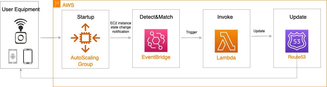
    CFN_REGION=ca-central-1
  3. Run the following command to encrypt the image using the AWS KMS key “EnclaveKMSKey”, make sure to replace “ca-central-1” with the region where you deployed your CloudFormation template:
    python3 ./envelope-encryption/encryptor.py --filePath ./images/air-show.jpg --cmkId alias/EnclaveKMSkey --region $CFN_REGION
  4. Verify that the output contains: file encrypted? True
    Note: The previous command generates two files: an encrypted image file and an encrypted data key file. The data key file is generated so we can demonstrate an attempt from the parent instance at decrypting the data key.

Launching VSock Proxy

Launch the VSock Proxy which proxies requests from the Nitro Enclave to an external endpoint, in this case, to AWS KMS. Note the file vsock-proxy-config.yaml contains a list of endpoints which allow-lists the endpoints that an enclave can communicate with.

cd ~/aws-nitro-enclaves-ai-ml-object-detection/src
vsock-proxy 8001 "kms.$CFN_REGION.amazonaws.com" 443 --config vsock-proxy-config.yaml &

Object Detection using Nitro Enclaves

Send the encrypted image to the enclave to decrypt the image and use the AI/ML model to detect objects and return a summary of the objects detected:

cd ~/aws-nitro-enclaves-ai-ml-object-detection/src
python3 client.py --filePath ./images/air-show.jpg.encrypted | jq -C '.'

The previous step takes around a minute to complete when first called. Inside the enclave, the server application decrypts the image, runs it through the AI/ML model to generate a list of objects detected and returns that list to the client application.

Parent Instance Credentials

Attempt to Decrypt Data Key using Parent Instance Credentials

To prove that the parent instance is not able to decrypt the content, attempt to decrypt the image using the parent’s credentials:

cd ~/aws-nitro-enclaves-ai-ml-object-detection/src
aws kms decrypt --ciphertext-blob fileb://images/air-show.jpg.data_key.encrypted --region $CFN_REGION

Note: The command is expected to fail with AccessDeniedException, since the parent instance is not allowed to decrypt the data key.

Cleaning up

  1. Open the AWS CloudFormation console at: https://console.aws.amazon.com/cloudformation/.
  2. Select the stack you created earlier, such as NitroEnclaveStack.
  3. Choose Delete, then choose Delete Stack.
  4. The stack status is initially DELETE_IN_PROGRESS. Click the Refresh button periodically to refresh its status. The status changes to DELETE_COMPLETE after it’s finished and the stack name no longer appears in your list of active stacks.

Conclusion

In this post, we showcase how to process sensitive data with Nitro Enclaves using an AI/ML model deployed on Amazon EC2, as well as how to integrate an enclave with AWS KMS to restrict access to an AWS KMS CMK so that only the Nitro Enclave is allowed to use the key and decrypt the image.

We encrypt the sample data with envelope encryption to illustrate how to protect, transfer and securely process highly sensitive data. This process would be similar for any kind of sensitive information such as personally identifiable information (PII), healthcare or intellectual property (IP) which could also be the AI/ML model.

Dig deeper by exploring how to further restrict your AWS KMS CMK using additional PCR hashes such as PCR1 (hash of the Linux kernel and bootstrap), PCR2 (Hash of the application), and other hashes available to you.

Also, try our comprehensive Nitro Enclave workshop which includes use-cases at different complexity levels.