Tag Archives: AWS Lambda

Improving throughput of serverless streaming workloads for Kafka

Post Syndicated from Anton Aleksandrov original https://aws.amazon.com/blogs/compute/improving-throughput-of-serverless-streaming-workloads-for-kafka/

Event-driven applications often need to process data in real-time. When you use AWS Lambda to process records from Apache Kafka topics, you frequently encounter two typical requirements: you need to process very high volumes of records in close to real-time, and you want your consumers to have the ability to scale rapidly to handle traffic spikes. Achieving both necessitates understanding how Lambda consumes Kafka streams, where the potential bottlenecks are, and how to optimize configurations for high throughput and best performance.

In this post, we discuss how to optimize Kafka processing with Lambda for both high throughput and predictable scaling. We explore the Lambda’s Kafka Event Source Mappings (ESMs) scaling, optimization techniques available during record consumption, how to use ESM Provisioned Mode for bursty workloads, and which observability metrics you need to use for performance optimization.

Overview

To start processing records from a Kafka topic with a Lambda function, whether using Amazon Managed Streaming for Apache Kafka (Amazon MSK) or a self-managed Kafka cluster, you create an ESM: a lightweight serverless resource that consumes records from Kafka topics and invokes your function.

The scaling behavior of Kafka ESMs is based on the offset lag. This is a metric indicating the number of records in the topic that have not yet been consumed by the Lambda function. This metric typically grows when producers publish new records faster than consumers process them. As the lag grows, the Lambda service gradually adds more Kafka consumers (also known as pollers) to your ESM. To preserve ordering guarantees, the maximum number of pollers is capped by the number of partitions in the topic. Lambda also scales pollers down automatically when lag decreases.

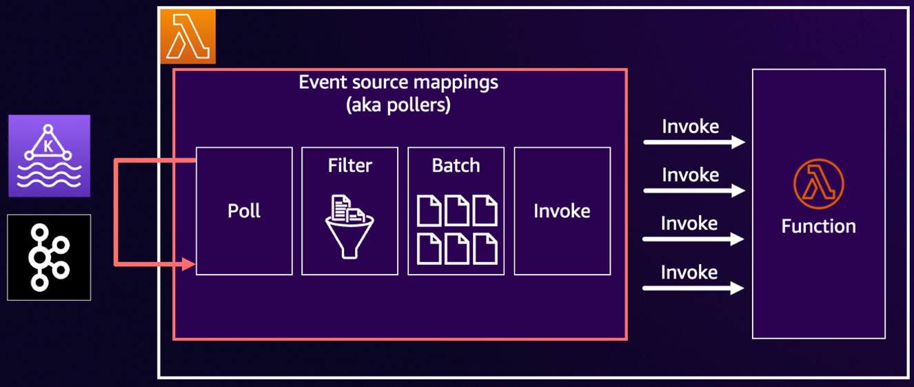
Each ESM follows a consistent polling workflow: poll -> filter -> batch -> invoke, as shown in the following diagram. Every stage has configurable options that directly affect performance, latency, and cost.


Figure 1. ESM processing workflow.

Polling: Increasing predictability with Provisioned Mode

By default, Kafka ESM uses the on-demand polling mode. In this mode, ESM starts with one poller, automatically adds more pollers when the offset lag grows, and scales the number of pollers down as lag decreases. On-demand mode does not need upfront scaling configuration and is the lowest-cost option for steady workloads. For many applications, this behavior is sufficient: scaling up can take several minutes, but the throughput eventually catches up, and you only pay for the resources you use, such as number of invocations.

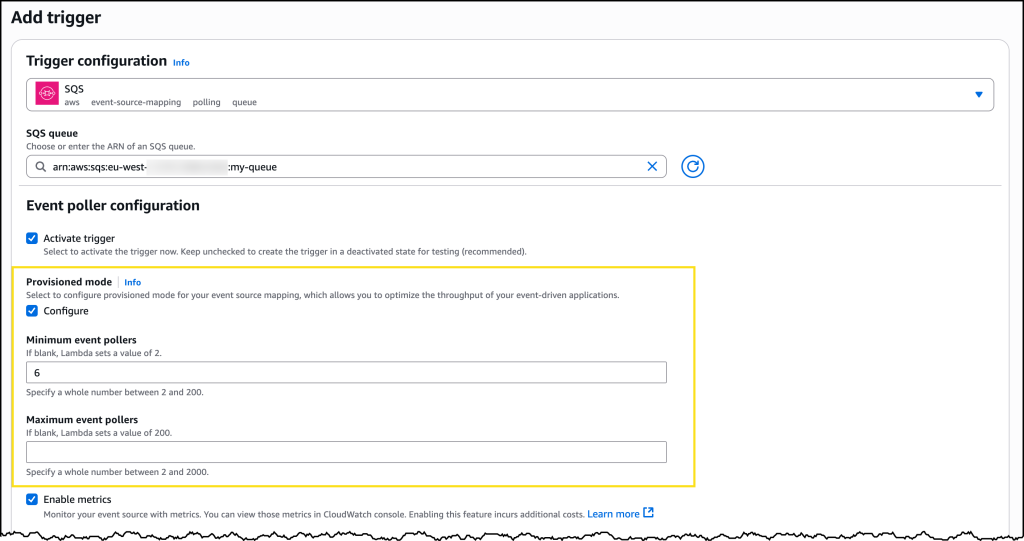
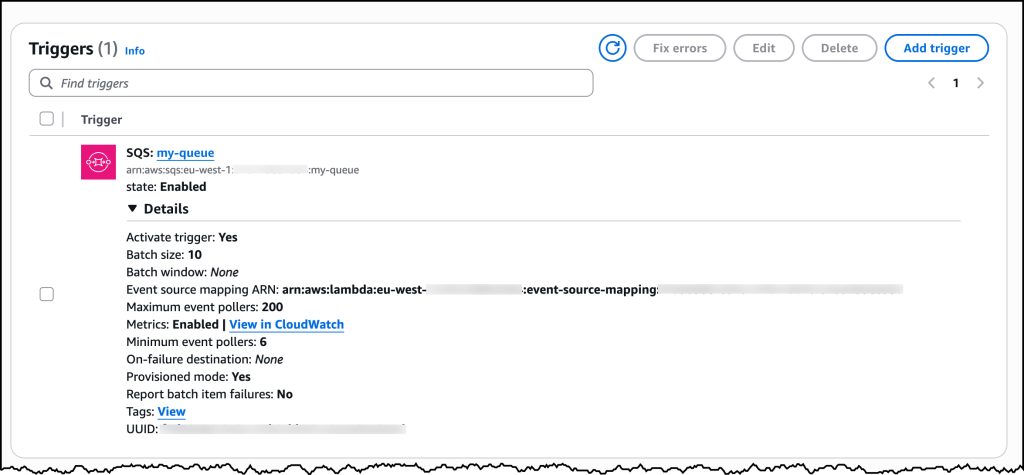
However, if your workloads are bursty and latency-sensitive, then on-demand scaling may not be fast enough and can result in a rapidly growing lag. This can be addressed by switching to Provisioned Mode, which gives you more fine-grained control to configure a minimum and maximum number of always-on pollers for your Kafka ESM. These pollers remain connected even when traffic is low, so consumption begins immediately when a spike occurs, and scaling within the configured range is faster and more predictable.

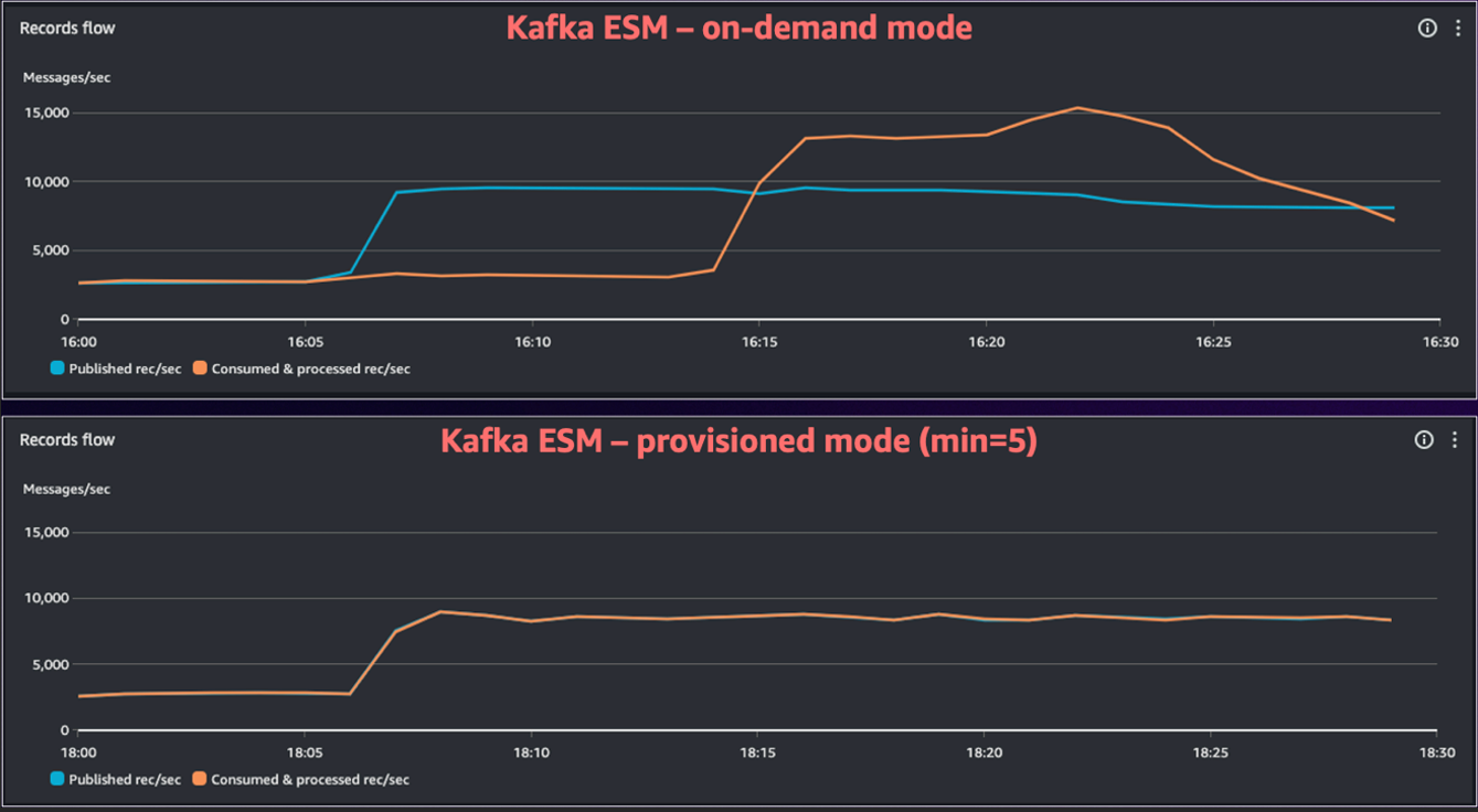
The following diagram shows the performance improvements of using the ESM in Provisioned Mode for bursty workloads. You can see that in on-demand mode it took ESM over 15 minutes to eventually catch up to the new traffic volume, while in Provisioned Mode the ESM handled the traffic increase instantly.


Figure 2. Comparing Kafka ESM on-demand and Provisioned Mode.

Best practices for using Provisioned Mode:

  • Start small: Provisioned Mode is a paid capability. AWS recommends that for smaller topics (less than 10 partitions) you start with a single provisioned poller to evaluate throughput and observe workload behavior. For larger topics, you can start with a higher number of provisioned pollers to accommodate the baseline consumption. You can adjust this configuration at any time as you learn traffic patterns and refine your performance targets.
  • Estimate throughput: A single provisioned poller can process up to 5 MB/s of Kafka data. Monitor your average record size and per-record processing time to establish a baseline for minimum and maximum pollers, then validate with real workload metrics.
  • Set a low floor and flexible ceiling: Choose a minimum number of pollers that makes sure that latency targets are met when a traffic burst occurs, then allow the ESM to scale toward a higher maximum as needed.

See Low latency processing for Kafka event sources for more information.

To summarize:

  • Use Provisioned Mode for bursty traffic, strict SLOs, or when backlogs pose downstream risk.
  • Use on-demand polling mode for steady traffic, flexible latency requirements, or when minimizing cost is the primary objective.

Filtering: Drop irrelevant records early

By default, all records from Kafka are delivered to your Lambda function. This approach is direct and flexible. Your handler code decides which records to process and which to ignore. This default behavior is highly efficient for workloads where nearly all records are valuable.

When you find yourself discarding a large portion of records in your handler code, you can use native ESM filtering capabilities to drop irrelevant records before they reach your function. You can filter early to reduce cost, free up concurrency, increase throughput, and make sure that your Lambda function spends cycles on valuable work only.

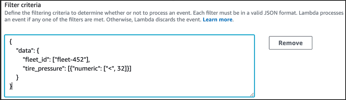
The following diagram shows the application of an ESM filter to only process telemetry that meets a specified condition.


Figure 3. ESM filtering configuration.

Batching: Processing more records per invocation

You can batch multiple Kafka records together to process more data per invocation and increase the efficiency of your Lambda functions. Larger batches help you achieve higher throughput and reduce costs by making better use of each invocation run. To get the best results, you should balance batch size and latency targets and adjust the configuration based on your workload’s specific traffic patterns and SLOs.

Lambda gives you two primary controls for configuring ESM batching behavior:

  • Batch window: This is how long the ESM waits to accumulate records before invoking your function. A shorter window produces smaller batches and more frequent invocations. A longer window (up to 5 minutes) produces larger batches and less frequent invocations.
  • Batch size: This is the maximum number of records that the ESM can accumulate before invoking your function, up to 10,000.

There’s no single setting that universally works for all workloads. Your optimal configuration depends on workload characteristics such as latency tolerance and record size. AWS recommends starting with the default values and then gradually adjusting the configuration based on your requirements. For example, you can increase the batch size while monitoring function duration, error rates, and end-to-end latency.

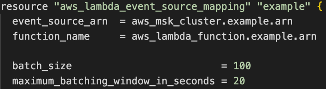
The following diagram shows how to configure batch window and size using Terraform:


Figure 4. ESM batch window and batch size configuration with Terraform.

The ESM invokes your function when one of the following three conditions is met:

  1. The batch window elapses.
  2. The accumulated batch reaches the configured maximum batch size.
  3. The accumulated payload approaches the 6 MB maximum invocation payload limit of Lambda.

When using higher batch window values during traffic spikes, you typically see more records-per-batch and longer function invocation durations. This is normal: larger batches can take longer to process. Always interpret the Duration metric in the context of the batch size being processed.

Invoke: Process each batch faster and more efficiently

You control how quickly each batch completes through two main factors: the efficiency of your function code and the compute resources you allocate to your functions. You can improve both to process more records per second, reduce the necessary concurrency, and lower cost.

Optimize your code: Review your function handler code to identify where you can reduce work per record. For example, eliminate redundant serialization, initialize dependencies once during function startup, and consider parallel processing within the handler (where applicable). For performance-critical workloads, you can also choose languages that compile to binary, such as Go or Rust, which typically deliver high performance with lower resource usage.

Tune compute resources: Increasing the memory function allocation proportionally increases vCPU. Use the Lambda PowerTuning tool to find the memory configuration that best balances performance and cost for your workload.

Correlate metrics: As you optimize, monitor Duration and Concurrency. You should see the concurrency drop as duration improves. That correlation confirms that your changes are improving the system throughput and efficiency.

When you combine handler optimizations with early filtering and efficient batching, even small improvements can make your pipeline noticeably faster to operate under load.

Observability drives good decisions

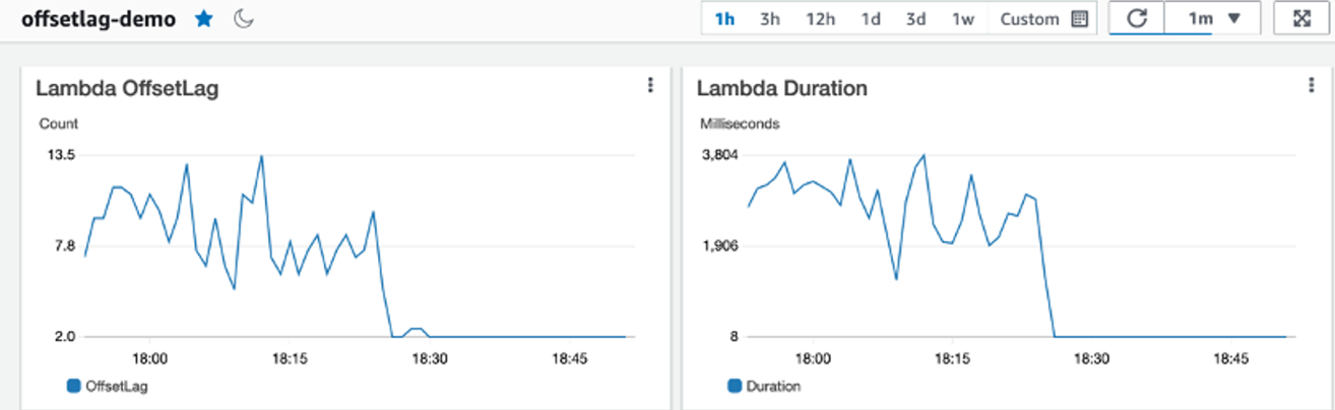
You can’t optimize what you can’t see. To tune your data processing pipeline, use a combination of OffsetLag, function invocation metrics, and Kafka broker metrics to understand your data processing performance. OffsetLag tells you whether your function is keeping up with incoming records, as shown in the following figure. Function metrics such as Duration, Concurrency, Errors, and Throttles show how efficiently your code is processing record batches. If you use Provisioned Mode, then you can use the Provisioned Pollers metric to track the poller capacity.


Figure 5. Kafka consumption observability with Amazon CloudWatch.

Always interpret function duration in the context of batch size. During traffic spikes, you can typically observe both duration and actual batch size increase, which is expected amortization, not a regression. For alerting, monitor lag growth, unexpected drops in invocation rate, and error spikes. With these signals in place, you can detect issues early and tune your configuration with confidence.

A sample step-by-step optimization loop

  1. Establish a clean baseline: Make your handler idempotent and batch-aware, start with a short batch window and moderate batch size. Monitor your ESM and confirm offset lag stays near zero at steady state.
  2. Filter early: Move static checks (record type, version, other custom properties) into ESM filtering and verify invoked counts drop relative to polled counts, proving the filter saves cost and concurrency.
  3. Increase batch size gradually while monitoring the duration, error rates, and latency metrics. Extend the batch window slightly if spikes cause too many invocations.
  4. Speed up the handler: Increase memory for more CPU, reduce per-record I/O, remove redundant serialization, and parallelize safely inside the batch while tracking duration and concurrency metrics together.
  5. Prove spike readiness: Replay realistic surges, monitor offset lag and drain time, and enable Provisioned Mode with a small minimum if recovery takes too long, adjusting with MB/s-per-poller estimates.
  6. Implement alerting: Watch for sustained lag growth, unexpected gaps between polled and invoked, and error spikes tied to partitions or large batches. Always read metrics in context with batch size.
  7. Re-evaluate periodically: Re-measure system throughput, confirm filter effectiveness, and retune batch and memory settings regularly as workloads evolve.

Conclusion

Optimizing Kafka streams processing with AWS Lambda necessitates understanding how ESMs work and tuning consumption components: polling, filtering, batching, and invoking. Filtering redundant records early removes unnecessary work, batching helps you process more records per invocation, and handler optimizations make sure that you make the most of the compute that you allocate. Together, these adjustments let you scale efficiently and keep offset lag under control.

When your workload is bursty, use Provisioned Mode to absorb spikes without long recovery times. With the right alerts on lag, errors, and unexpected polled versus invoked behavior, you can spot problems early and adjust before they impact users. Following this optimization guide gives you a practical way to measure, tune, and revisit your setup as traffic patterns change.

To learn more about optimizing Kafka consumption, see the AWS re:Invent 2024 session about Improving throughput and monitoring of serverless streaming workloads.

To learn more about building Serverless architectures see Serverless Land.

Serverless strategies for streaming LLM responses

Post Syndicated from KyungYong Shim original https://aws.amazon.com/blogs/compute/serverless-strategies-for-streaming-llm-responses/

Modern generative AI applications often need to stream large language model (LLM) outputs to users in real-time. Instead of waiting for a complete response, streaming delivers partial results as they become available, which significantly improves the user experience for chat interfaces and long-running AI tasks. This post compares three serverless approaches to handle Amazon Bedrock LLM streaming on Amazon Web Services (AWS), which helps you choose the best fit for your application.

  1. AWS Lambda function URLs with response streaming
  2. Amazon API Gateway WebSocket APIs
  3. AWS AppSync GraphQL subscriptions

We cover how each option works, the implementation details, authentication with Amazon Cognito, and when to choose one over the others.

Lambda function URLs with response streaming

AWS Lambda function URLs provide a direct HTTP(S) endpoint to invoke your Lambda function. Response streaming allows your function to send incremental chunks of data back to the caller without buffering the entire response. This approach is ideal for forwarding the Amazon Bedrock streamed output, providing a faster user experience. Streaming is supported in Node.js 18+. In Node.js, you wrap your handler with awslambda.streamifyResponse(), which provides a stream to write data to, and which sends it immediately to the HTTP response.

Architecture

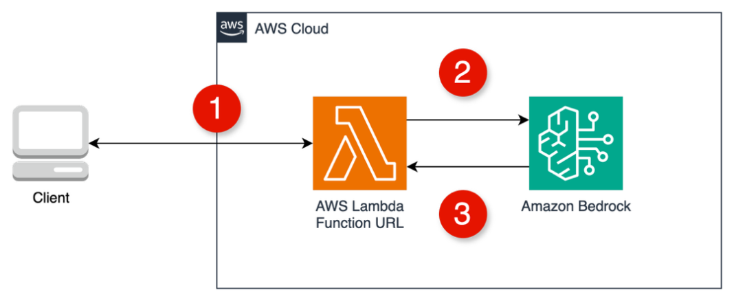
The following figure shows the architecture.

Lambda function URLs with Amazon Bedrock architecture

  1. The client makes a fetch() call to the Lambda function URL.
  2. Lambda invokes InvokeModelWithResponseStream using the AWS SDK for JavaScript.
  3. As tokens arrive from Amazon Bedrock, they are written to the response stream.

Implementation steps

  1. Create a streaming Lambda function: Use a Node.js 18+ or later runtime (necessary for native streaming). Install the AWS SDK to call Amazon Bedrock. In the handler code, wrap the function with awslambda.streamifyResponse and stream the model output. For example, in Node.js you might do the following:
    const bedrock = new BedrockRuntimeClient({region: “us-east-1”});
    
    // Please consider adding more details when you use it for your application.
    exports.handler = awslambda.streamifyResponse(async (event, responseStream) => 
    {
        // 1. Parse input (e.g., prompt from event)
        const prompt = event.body?.prompt;
        // 2. Call Amazon Bedrock with streaming (using AWS SDK for Amazon Bedrock)
        const command = new InvokeModelWithResponseStreamCommand({ modelId: "YOUR_MODEL_ID", body: { prompt }});
        const response = await bedrock.send(command);
        // 3. Stream Bedrock tokens to client
        for await (const event of response.body) {
            if (event.content) {
                responseStream.write(event.content); // write partial output
            }
        }
        // 4. End stream when done
        responseStream.end();
    });
    

  2. This code snippet uses the Amazon Bedrock SDK’s async iterable to read the event stream of tokens and writes each to the responseStream.
  3. Configure the Lambda role: the execution role must allow the Amazon Bedrock invocation (such as bedrock:InvokeModelWithResponseStream on the LLM model Amazon Resource Name (ARN)).

Authentication with Amazon Cognito

Lambda function URLs can be set to “None” (public) or “AWS_IAM”. Native Cognito User Pool token authentication isn’t supported, thus you need to implement a solution.

  1. JWT verification in Lambda: Allow public access and verify a valid JWT from Amazon Cognito in the request header within your Lambda code. This necessitates development effort.
    // Initialize Cognito JWT Verifier
    const { CognitoJwtVerifier } = require('aws-jwt-verify');
    
    const jwtVerifier = CognitoJwtVerifier.create({
      userPoolId: USER_POOL_ID,
      tokenUse: 'id',
      clientId: USER_POOL_CLIENT_ID
    });
    
    // Verify JWT token from Cognito
    async function verifyToken(token) {
      try {
        if (!token) throw new Error('No authorization token provided');
        
        // Remove 'Bearer ' prefix if present
        if (token.startsWith('Bearer ')) {
          token = token.slice(7);
        }
    
        // Verify the token using Cognito JWT Verifier
        const payload = await jwtVerifier.verify(token);
        logger.info(`Verified token for user: ${payload.sub}`);
        
        return payload;
      } catch (error) {
        logger.error(`Token verification failed: ${error.message}`);
        throw new Error(`Invalid token: ${error.message}`);
      }
    }
    
    //...
    
        // Verify authentication
        let userId;
        try {
          const authHeader = event.headers?.Authorization;
          const payload = await verifyToken(authHeader);
          userId = payload.sub;
          logger.info(`Authenticated user: ${userId}`);
        } catch (error) {
          responseStream.write(`data: ${JSON.stringify({ type: 'error', error: 'Unauthorized', message: error.message })}\n\n`);
          return;
        }
    

  2. IAM authorization with Amazon Cognito identity: Use AWS credentials obtained from Amazon Cognito. A more complex setup, especially for web apps, is potentially overkill for a single function.

Pros and cons of Lambda function URLs

Pros:

  • Clarity: No API Gateway or other services are needed, which minimizes operational overhead.
  • Low latency, high throughput: The response is delivered directly from Lambda to the client. This yields excellent Time To First Byte (TTFB) performance, with no intermediate buffering.
  • Direct implementation: For Node.js developers, enabling streaming is as direct as a wrapper and writing to a stream. This is ideal for quick prototypes or single function microservices.
  • Lower cost for low concurrent usage: You pay only for Lambda execution time. There’s no persistent connection cost, which is the same as with WebSocket or AWS AppSync. If invocations are infrequent or short, then this could be cost-efficient.

Cons:

  • Limited runtime support: Native streaming is only supported in Node.js.
  • No built-in user pool auth: Unlike API Gateway or AWS AppSync, Lambda URLs don’t directly support Amazon Cognito user pool authorizers. You must handle auth either through AWS Identity and Access Management (IAM) or manual token validation, adding some development effort and potential security pitfalls if done incorrectly.
  • Error handling complexity: Streaming makes error propagation trickier. If an error occurs mid-stream, then you need to decide how to inform the client.

API Gateway WebSocket for streaming

API Gateway WebSocket APIs establish persistent, stateful connections between clients and your backend. This is ideal for real-time applications needing server-initiated messages. The client connects once, sends a prompt to Amazon Bedrock through the WebSocket, and the server pushes the streamed response back over the same connection.

Architecture

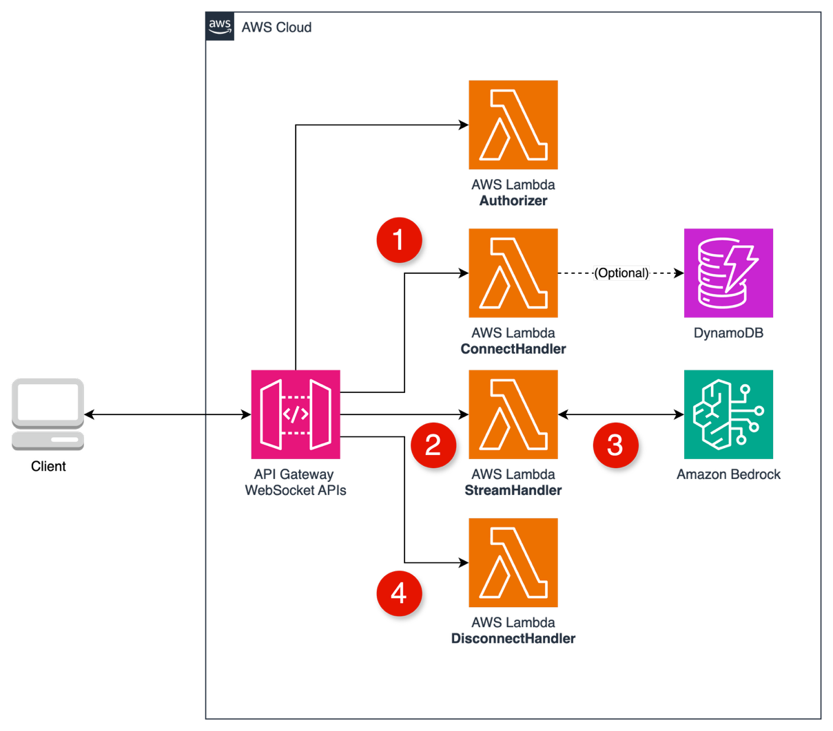
The following figure shows the architecture.

API Gateway WebSocket with Amazon Bedrock architecture

  1. Client connects through the WebSocket URL and store connectionId.
  2. Client sends a prompt through a custom route to the LLMHandler.
  3. Lambda as LLMHandler invokes Amazon Bedrock and streams back through WebSocket.
  4. Client disconnects through the DisconnectHandler and removes connectionId.

Implementation steps

  1. Create a WebSocket API in API Gateway with routes
    1. $connect: Connected to ConnectHandler Lambda.
    2. $disconnect: Connected to DisconnectHandler Lambda.
    3. $stream: All messages go to StreamHandler Lambda.
  2. Create Lambda Authorizer
    1. Receives the connection request with token in query string.
    2. Validates the JWT token against Amazon Cognito.
    3. Returns Allow/Deny policy for the connection.
      def lambda_handler(event, context):
          # Extract token from querystring
          token = event.get("queryStringParameters", {}).get("token", "")
          
          # Validate JWT token against Cognito
          if validate_token(token):
              return {
                  "isAuthorized": True,
                  # Optionally include context that other handlers can access
                  "context": {
                      "userId": extracted_user_id
                  }
              }
          else:
              return {"isAuthorized": False}
      

  3. Create Connection Handler
    1. Connection Lambda runs after successful authorization.
    2. Receives the new connection’s unique connectionId.
    3. Store connection info in Amazon DynamoDB (optional).
    4. Returns 200 status to complete the connection.
      def lambda_handler(event, context):
          # Extract connectionId
          connection_id = event.get("requestContext", {}).get("connectionId")
          
          # Optionally store in DynamoDB
          # dynamodb.put_item(...)
          
          # Connection established successfully
          return {"statusCode": 200}
      

  4. Create Disconnect Handler
    1. Disconnect Lambda is triggered automatically when clients disconnect.
    2. Receives the terminated connection’s connectionId.
    3. Cleans up any stored connection data.
    4. Returns 200 status
      def lambda_handler(event, context):
          # Extract connectionId
          connection_id = event.get("requestContext", {}).get("connectionId")
          
          # Optionally remove from DynamoDB
          # dynamodb.delete_item(...)
          
          # Disconnection handled successfully
          return {"statusCode": 200}
      

  5. Create LLM Handler
      1. Receives messages sent to the stream route.
      2. Extracts prompt from the message body.
      3. Calls Amazon Bedrock model with streaming response.
      4. Streams tokens back to the client using the connection ID.
        def lambda_handler(event, context):
            # Extract connectionId and domain details for sending responses
            connection_id = event["requestContext"]["connectionId"]
            domain = event["requestContext"]["domainName"]
            stage = event["requestContext"]["stage"]
            
            # Parse message body to get the prompt
            body = json.loads(event.get("body", "{}"))
            prompt = body.get("prompt", "")
            
            # Create API Gateway management client for sending responses
            api_client = boto3.client(
                'apigatewaymanagementapi',
                endpoint_url=f'https://{domain}/{stage}'
            )
            
            # Call Amazon Bedrock with streaming response
            response = bedrock_client.invoke_model_with_response_stream(...)
            
            # Stream tokens back to client
            for chunk in response["body"]:
                # Extract token from chunk
                token = process_chunk(chunk)
                
                # Send token directly back through the WebSocket
                api_client.post_to_connection(
                    ConnectionId=connection_id,
                    Data=json.dumps({"token": token, "isComplete": False})
                )
            
            # Send completion message
            api_client.post_to_connection(
                ConnectionId=connection_id,
                Data=json.dumps({"token": "", "isComplete": True})
            )
            
            return {"statusCode": 200}
        

Authentication with Amazon Cognito

Securing a WebSocket API with Amazon Cognito needs a bit more work. API Gateway WebSocket doesn’t have a built-in Amazon Cognito User Pool authorizer:

  1. Lambda authorizer with JWT authentication: API Gateway invokes your Lambda authorizer upon connection, validating the Amazon Cognito JWT (passed as a query parameter). The Lambda generates an IAM policy granting access and returns it.
  2. IAM authentication for WebSockets: Clients sign requests with SigV4 using AWS credentials from an Amazon Cognito Identity Pool. API Gateway evaluates the request against IAM policies.

Pros and cons of API Gateway WebSocket APIs

Pros:

  • Bidirectional real-time communication: WebSockets are ideal for applications where the server needs to push data such as the LLM’s response without explicit requests.
  • Persistent connection for multi-turn conversations: After the initial handshake, the same connection can be reused for subsequent prompts and responses, avoiding repeated setup latency. This is great for a chat UI where the user asks multiple questions in one session.
  • Scalability: API Gateway is a managed service that can handle 500 connections/second and 10,000 requests/second across APIs, which can be increased by request.

Cons:

  • Higher development complexity: When compared to the clarity of a direct Lambda URL, a WebSocket API involves multiple Lambdas and coordination to manage the connection state.
  • Custom auth implementation: There is no built-in Amazon Cognito user pool integration, thus you must implement a Lambda authorizer.
  • Timeout management: The API Gateway integration timeout is 29 s, thus your Lambda function should return the response promptly.

AWS AppSync GraphQL subscription

AWS AppSync is a fully managed GraphQL service that streamlines building real-time APIs. It handles WebSocket connections and client fan-out automatically. Clients subscribe to a GraphQL subscription, and a Lambda resolver pushes the Amazon Bedrock streamed tokens back.

Architecture

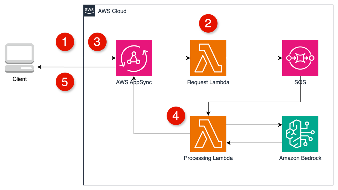
The following figure shows the architecture.

AWS AppSync GraphQL subscription with Amazon Bedrock architecture

  1. Client calls a startStream mutation. AppSync invokes the Request Lambda.
  2. The Request Lambda immediately returns a unique sessionId and sends the processing task to an Amazon Simple Queue Service (Amazon SQS) queue.
  3. Client uses the sessionId to subscribe to an onTokenReceived GraphQL subscription.
  4. The Processing Lambda (triggered by Amazon SQS) invokes Amazon Bedrock and, for each token, calls a publishToken mutation in AWS AppSync.
  5. AWS AppSync automatically pushes the token to all clients subscribed with the matching sessionId.

Implementation steps

  1. Design the GraphQL Schema: define types and operations.
    type StreamResponse {
      sessionId: String!
      status: String!
      message: String
      timestamp: String!
      error: String
    }
    
    type TokenEvent {
      sessionId: String!
      token: String!
      isComplete: Boolean!
      timestamp: String!
    }
    
    type Mutation {
      startStream(prompt: String!): StreamResponse!
      publishToken(sessionId: String!, token: String!, isComplete: Boolean!): TokenEvent!
    }
    
    type Subscription {
      onTokenReceived(sessionId: String!): TokenEvent
    

  2. Create the Request Handler (Request Lambda)
    1. Receives the GraphQL mutation with the prompt.
    2. Generates a unique session ID.
    3. Sends the prompt and session ID to the SQS queue.
    4. Returns the session ID to the client immediately.
      def lambda_handler(event, context):
          # Extract prompt from GraphQL event
          prompt = event["arguments"]["prompt"]
          
          # Generate unique session ID
          session_id = str(uuid.uuid4())
          
          # Send message to SQS queue
          sqs_client.send_message(
              QueueUrl="your-sqs-queue-url",
              MessageBody=json.dumps({
                  "prompt": prompt,
                  "sessionId": session_id
              })
          )
          
          # Return session ID to client
          return {
              "sessionId": session_id,
              "status": "streaming_started",
              "timestamp": datetime.datetime.utcnow().isoformat()
          }
      

  3. Create the Processing Handler (Processing Lambda)
    1. It is triggered by Amazon SQS messages.
    2. It calls Amazon Bedrock with streaming enabled.
    3. For each token generated, it calls the AppSync publishToken mutation.
      def lambda_handler(event, context):
          # Process SQS event records
          for record in event["Records"]:
              body = json.loads(record["body"])
              prompt = body["prompt"]
              session_id = body["sessionId"]
              
              # Call Amazon Bedrock with streaming
              response = bedrock_client.invoke_model_with_response_stream(...)
              
              # Process streaming response
              for chunk in response["body"]:
                  # Extract token from chunk
                  token = process_chunk(chunk)
                  
                  # Publish token to AppSync
                  publish_token_to_appsync(
                      session_id=session_id,
                      token=token,
                      is_complete=False
                  )
              
              # Send completion token
              publish_token_to_appsync(
                  session_id=session_id,
                  token="",
                  is_complete=True
              )
      

  4. Configure GraphQL Resolvers
    1. StartStream resolver: Connect to the Request Lambda.
    2. PublishToken resolver: Trigger subscription with a NONE data source.
  5. Client subscription setup
    1. Make a startStream mutation.
      const { sessionId } = await client.mutate({
        mutation: START_STREAM,
        variables: { prompt }
      });
      

    2. Subscribe to receive tokens.
      client.subscribe({
        query: ON_TOKEN_RECEIVED,
        variables: { sessionId }
      }).subscribe({
        next: ({ data }) => {
          if (data.onTokenReceived.isComplete) {
            // Handle completion
          } else {
            // Append token to UI
            appendToken(data.onTokenReceived.token);
          }
        }
      });
      

Authentication with Amazon Cognito

AWS AppSync integrates seamlessly with Amazon Cognito User Pools. Setting the API’s auth mode to Amazon Cognito User Pool needs a valid JWT for every GraphQL operation. This is the most developer-friendly option for authentication. AWS AppSync handles the handshake and token refresh.

Pros and cons of AWS AppSync subscriptions

Pros:

  • Fully managed real-time protocol: You don’t deal with raw WebSockets or connection IDs at all. AWS AppSync automatically establishes and maintains a secure WebSocket for subscriptions (no need for a connect or disconnect Lambda).
  • Streamlined authentication: Built-in support for Amazon Cognito User Pool tokens means that you can secure the API without writing custom authorizers.

Cons:

  • Potential overhead and complexity: For a direct case (one prompt—one stream), introducing GraphQL and AWS AppSync might be seen as over-engineering if your app doesn’t use GraphQL for other use cases.
  • 30-second resolver limit: AWS AppSync has a 30-second limit for mutation resolvers, thus you need to design the initial request to start the process and immediately return, relying on a subscription to stream the results progressively to avoid blocking the user.

Conclusion

The Amazon Bedrock streaming interface unlocks fluid, low-latency LLM experiences. You can use the right AWS serverless architecture to deliver streamed responses in a secure, scalable, and cost-effective way.

  • Lambda function URLs with streaming: Direct, single-user applications and prototypes.
  • API Gateway WebSocket: Multi-turn conversations, collaborative applications.
  • AppSync: Complex applications already using GraphQL.

Each method is serverless, production-ready, and fully integrated with Amazon Cognito for secure access control. AWS provides the flexibility to design high-quality AI user experiences at scale.

Refer to GitHub sample source code for more details.

Comparative table

Feature LAMBDA FUNCTION URLS API GATEWAY WEBSOCKET APIs APPSYNC GRAPHQL SUBSCRIPTIONS
Complexity Lowest Medium High
Real-time focus Limited Strong Strong
Authentication Needs custom logic Needs custom logic Built-in Amazon Cognito support
Scalability Good Good Excellent
GraphQL support None None Native
Use cases Q&A Chatbots, real-time apps Complex apps, multi-user scenarios
Cost Pay per invocation Connection time and Lambda execution Request/connection-based pricing


Building multi-tenant SaaS applications with AWS Lambda’s new tenant isolation mode

Post Syndicated from Anton Aleksandrov original https://aws.amazon.com/blogs/compute/building-multi-tenant-saas-applications-with-aws-lambdas-new-tenant-isolation-mode/

Today, AWS announced a new tenant isolation mode for AWS Lambda, that allows you to process function invocations in separate execution environments for each application end-user or tenant invoking your Lambda function. This capability simplifies building secure multi-tenant SaaS applications by managing tenant-level compute environment isolation and request routing for you. As a result, you can focus on your core business logic rather than implementing your own tenant-aware compute environment isolation.

Overview

Lambda runs your function code in secure execution environments that leverage Firecracker virtualization to provide isolation. These execution environments never share or reuse virtual resources (such as vCPU, disk, or memory) across functions, or even across different versions of the same function. However, Lambda can reuse execution environments for multiple invocations of the same function version, as these execution environments are fully set-up and can therefore deliver faster request processing for your functions.

Figure 1. Incoming invocations processed by a collection of execution environments that belong to a single function.

Figure 1. Incoming invocations processed by a collection of execution environments that belong to a single function.

Multi-tenant SaaS applications that handle sensitive tenant-specific data or execute code supplied dynamically by tenants may need a higher degree of isolation—at the individual application tenant level rather than at the function level—for secure code execution and to reduce the risk of cross-tenant data access.

Prior to today’s launch, developers would implement custom solutions, such as SDKs or application logic to manage isolation within function code. This approach was bug-prone, required more work from application development teams, and didn’t ensure isolation at the compute environment level.

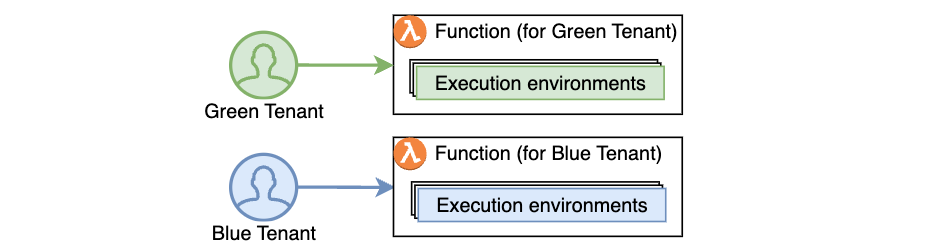
Alternatively, developers adopted the approach of creating separate functions per application tenant, replicating the same code across hundreds or thousands of tenants. This approach provided stronger compute environment isolation than sharing compute environments across multiple tenants of the same function, but increased implementation overhead and operational complexity as workloads grew to support a larger number of tenants over time.

Figure 2. Using function-per-tenant model, each tenant’s requests are processed by a separate function.

Figure 2. Using function-per-tenant model, each tenant’s requests are processed by a separate function.

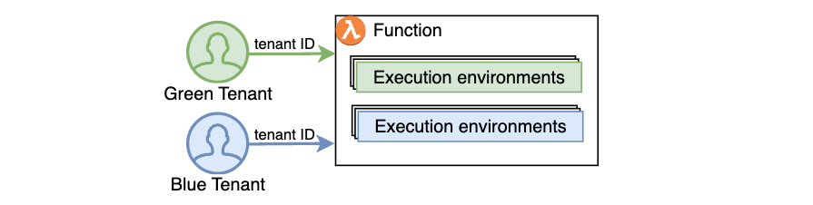
Starting today, AWS Lambda offers a new tenant isolation mode that lets you isolate execution environments used across different tenants of your multi-tenant SaaS applications, even when all of the tenants invoke the same function. When you enable the new tenant isolation mode, you include a tenant identifier with each function invocation. Lambda uses this identifier to route the request to the correct execution environment. As a result, each execution environment is reused only for invocations from the same tenant. This means you still get the performance benefits of warm execution environments, while ensuring that each tenant’s workloads remain isolated.

Figure 3. With the new tenant isolation capability, Lambda creates separate execution environments per tenant for a single function.

Figure 3. With the new tenant isolation capability, Lambda creates separate execution environments per tenant for a single function.

For organizations handling sensitive tenant-specific data or running untrusted code supplied dynamically by end-users, Lambda’s new tenant isolation mode provides the security benefits of per-tenant compute environment separation without the operational complexity of managing individual functions or infrastructure for each tenant.

Example scenario

Consider building a multi-tenant serverless SaaS application. To optimize performance, your function handler can retrieve tenant-specific configuration and data, cache it in memory, and reuse it for subsequent invocations from the same tenant. For example, you might cache tenant-specific database location, feature flags, or business rules that are frequently accessed during request processing. You may store this information within the application runtime process as global variables or as files in the /tmp directory. However, if the underlying execution environment is used to serve multiple tenants, this approach can potentially expose data across tenants.

With tenant isolation mode you can address this risk with much simpler architecture and configuration. This built-in capability makes Lambda an excellent choice for multi-tenant SaaS applications needing isolated compute environments for individual tenants.

Getting Started with Lambda Tenant Isolation Mode

Use the new tenancy-config parameter to configure tenant isolation mode when you create your function. You can only apply this configuration at function creation time; it cannot be updated for existing functions. The following snippet creates a function with tenancy config using the AWS CLI.

aws lambda create-function \
   --function-name my-function1 \
   --runtime nodejs22.x \
   --zip-file fileb://my-function1.zip \
   --handler index.handler \
   --role arn:aws:iam:1234567890:role/my-function-role \
   --tenancy-config '{"TenantIsolationMode": "PER_TENANT"}'

After the function is created, you must provide the tenant ID parameter with each invocation. Lambda uses this identifier to ensure that the execution environment used for a particular tenant is never reused for other tenants. For subsequent invocations from the same tenant, Lambda may reuse the execution environment to optimize performance. Specify this tenant-id parameter as illustrated below:

aws lambda invoke \
   --function-name my-function \
   --tenant-id BlueTenant \
   response.json

The new tenant-id parameter is required for functions using the tenant isolation mode. Function invocations omitting this parameter will fail with an invocation error, as shown below:

aws lambda invoke --function-name multitenant-function out.json

An error occurred (InvalidParameterValueException) when calling the Invoke operation:
The invoked function is enabled with tenancy configuration. 
Add a valid tenant ID in your request and try again.

Lambda makes the tenant ID parameter available through your function handler’s context object. This allows you to access tenant-specific information in your code, for example if you wish to implement custom logic based on the tenant identity, as shown below:

exports.handler = async function (event, context) {
   const tenantId = context.tenantId;

   // Process tenant-specific logic

   return {
      statusCode: 200,
      body: `OK for tenantId=${tenantId}`
   };
};

The following table outlines differences between Lambda functions with and without tenant isolation mode enabled:

Feature Without the new
tenant isolation mode
With the new
tenant isolation mode
Execution environment isolation Isolated per function version. Isolated per end-user or tenant invoking a function version.
Execution environment reuse Can be reused to process all invocations of a function version. Can only be reused to process invocations from the same tenant invoking a function version.
Data stored on local disk and in-memory Potentially accessible across all invocations of a function version. Potentially accessible across invocations from the same tenant. Not accessible for invocations from other tenants.
Cold starts Occur when there are no warm execution environments available to process incoming invocation. Occur when there are no tenant-specific warm execution environments available to process incoming invocation. More cold starts expected due to tenant-specific execution environments.

Integrating with Amazon API Gateway

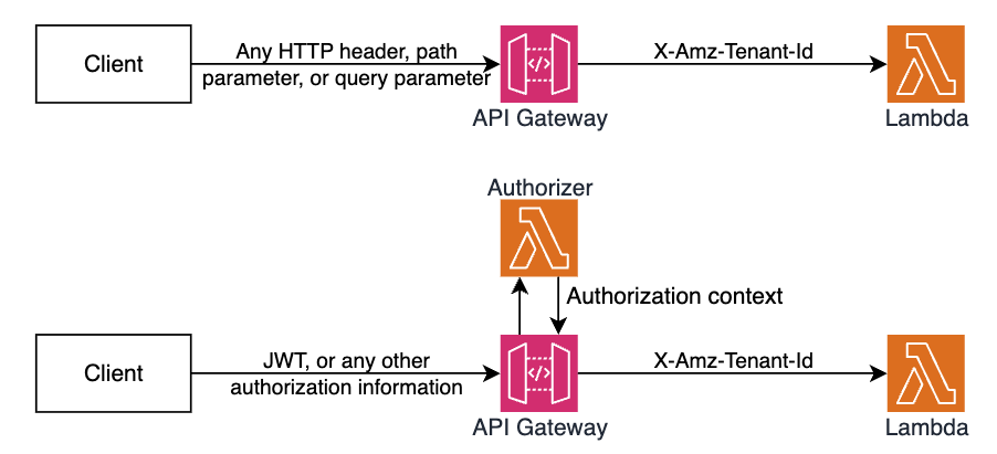
Amazon API Gateway uses Lambda’s Invoke API to invoke Lambda functions. When using the Invoke API, Lambda expects the tenant ID parameter to be passed using the X-Amz-Tenant-Id HTTP header. You can configure API Gateway to inject this HTTP header into the Lambda invocation request with a value obtained from client request properties such as HTTP header, query parameter, or path parameter. When using Lambda Authorizers, you can obtain the value from authorization context information returned by the authorizer, such as principal ID or JWT claim. See API Gateway documentation to learn how you can return authorization information from Lambda authorizers to be used for the X-Amz-Tenant-Id header value.

Figure 4. Obtaining X-Amz-Tenant-Id header value from authentication sources.

Figure 4. Obtaining X-Amz-Tenant-Id header value from authentication sources.

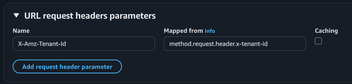
The following screenshot illustrates API Gateway Lambda integration configuration, where the incoming request to API Gateway includes an x-tenant-id header that is mapped to the X-Amz-Tenant-Id request header to invoke a Lambda function using tenant isolation mode.

Figure 5. Mapping client request header to Lambda tenant-id header.

Figure 5. Mapping client request header to Lambda tenant-id header.

The following code snippet illustrates this configuration implemented with the AWS CDK.

const lambdaIntegration = new ApiGw.LambdaIntegration(fn, {
   requestParameters: {
      // This configures API Gateway to inject X-Amz-Tenant-Id header
      // into downstream requests. The header value is obtained from 
      // x-tenant-id header in the client request.
      'integration.request.header.X-Amz-Tenant-Id': 'method.request.header.x-tenant-id'
   }
});

resource.addMethod('GET', lambdaIntegration, {
   requestParameters: {
      // This enables API Gateway to use the x-tenant-id header value 
      // obtained from the client request. The header name is arbitrary.
      // you can use any other header name. 
      'method.request.header.x-tenant-id': true
   }
});

Tenant-aware observability

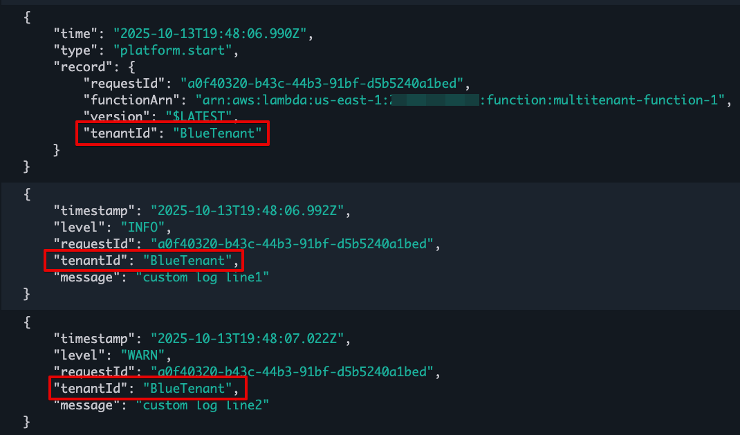
For functions using tenant isolation, Lambda automatically includes the tenant ID in function logs when you have JSON logging enabled, making it easier to monitor and debug tenant-specific issues. Note that the tenantId property is available during function invocation, rather than during function initialization. The tenantId property is included for both platform events (like platform.start and platform.report) and custom logs you print in your function code, as shown in the following screenshot:

Figure 6. Lambda function logs with tenantId.

Figure 6. Lambda function logs with tenantId.

Lambda creates a separate CloudWatch log stream for each execution environment. You can use CloudWatch Log Insights to find log streams that belong to a particular tenant by filtering by tenant Id:

fields @logStream, @message
| filter tenantId=='BlueTenant' or record.tenantId=='BlueTenant'
| stats count() as logCount by @logStream
| sort @timestamp desc

You can also retrieve tenant-specific logs across all log streams:

fields @message
| filter tenantId=='BlueTenant' or record.tenantId=='BlueTenant'
| limit 1000

Each log stream starts with function initialization logs followed by the invocation logs. This structure helps you to debug tenant-specific issues and understand the lifecycle of each tenant’s execution environments.

Considerations

When using the new tenant isolation for Lambda functions, consider the following:

  • Each tenant’s execution environments are isolated from other tenants so that tenant-specific data stored on disk or in memory remain separated from other tenants invoking the same Lambda function.
  • All tenants share the function’s execution role. For more fine-grained permissions for individual tenants, consider propagating tenant-scoped credentials from the upstream application components invoking your Lambda function.
  • Your application may experience higher percentage of cold starts, as Lambda processes requests in separate execution environments for each tenant invoking your functions.
  • You pay a fee for each new tenant-specific execution environment created, depending on the memory configured for your function. See Lambda pricing page for details.

Best practices

When using the new tenant isolation mode for Lambda functions, AWS recommends the following best practices:

  • Implement robust tenant ID validation at the application layer to prevent unauthorized access through tenant ID manipulation. Consider using a dedicated service or database to maintain valid tenant IDs.
  • Monitor and audit tenant access patterns regularly to detect potential security anomalies or unauthorized cross-tenant access attempts.
  • Be aware of Lambda concurrency quotas when building multi-tenant applications. You might need to request quota increases based on your tenant count and usage patterns.

Sample code

Follow the instructions in this GitHub repository to provision a sample project in your own account and see the new Lambda tenant isolation mode in action. The sample project illustrates how to integrate a function using the new tenant isolation mode with Amazon API Gateway and propagate tenant identity from client requests.

Conclusion

The new tenant isolation mode for Lambda simplifies building serverless multi-tenant SaaS applications on AWS. By automatically managing application tenant-level compute environment isolation, this capability eliminates the need for custom isolation logic or separate tenant functions, allowing you to focus on the core business logic while AWS handles the complexities of tenant-aware compute environment isolation.

Combined with the existing security features in Lambda, rapid scaling, and pay-per-use pricing, tenant isolation mode makes Lambda an even more compelling choice for modern SaaS applications, whether you’re building new solutions or enhancing existing ones.

To learn more, refer to the documentation for tenant isolation. For details on pricing, refer to Lambda’s pricing page.

Building responsive APIs with Amazon API Gateway response streaming

Post Syndicated from Anton Aleksandrov original https://aws.amazon.com/blogs/compute/building-responsive-apis-with-amazon-api-gateway-response-streaming/

Today, AWS announced support for response streaming in Amazon API Gateway to significantly improve the responsiveness of your REST APIs by progressively streaming response payloads back to the client. With this new capability, you can use streamed responses to enhance user experience when building LLM-driven applications (such as AI agents and chatbots), improve time-to-first-byte (TTFB) performance for web and mobile applications, stream large files, and perform long-running operations while reporting incremental progress using protocols such as server-sent events (SSE).

In this post you will learn about this new capability, the challenges it addresses, and how to use response streaming to improve the responsiveness of your applications.

Overview

Consider this scenario – you’re running an AI-powered agentic application that uses an Amazon Bedrock foundation model. Your users interact with the application through an API, asking complex questions that require detailed responses. Before response streaming, users would send their prompts and wait to eventually receive the application response, sometimes for tens of seconds. This awkward pause between questions and responses created a disconnected, unnatural experience.

With the new API Gateway response streaming capability, the interaction through the API becomes much more fluid and natural. As soon as your application starts processing the model response, you can stream it back to your users using the API Gateway.

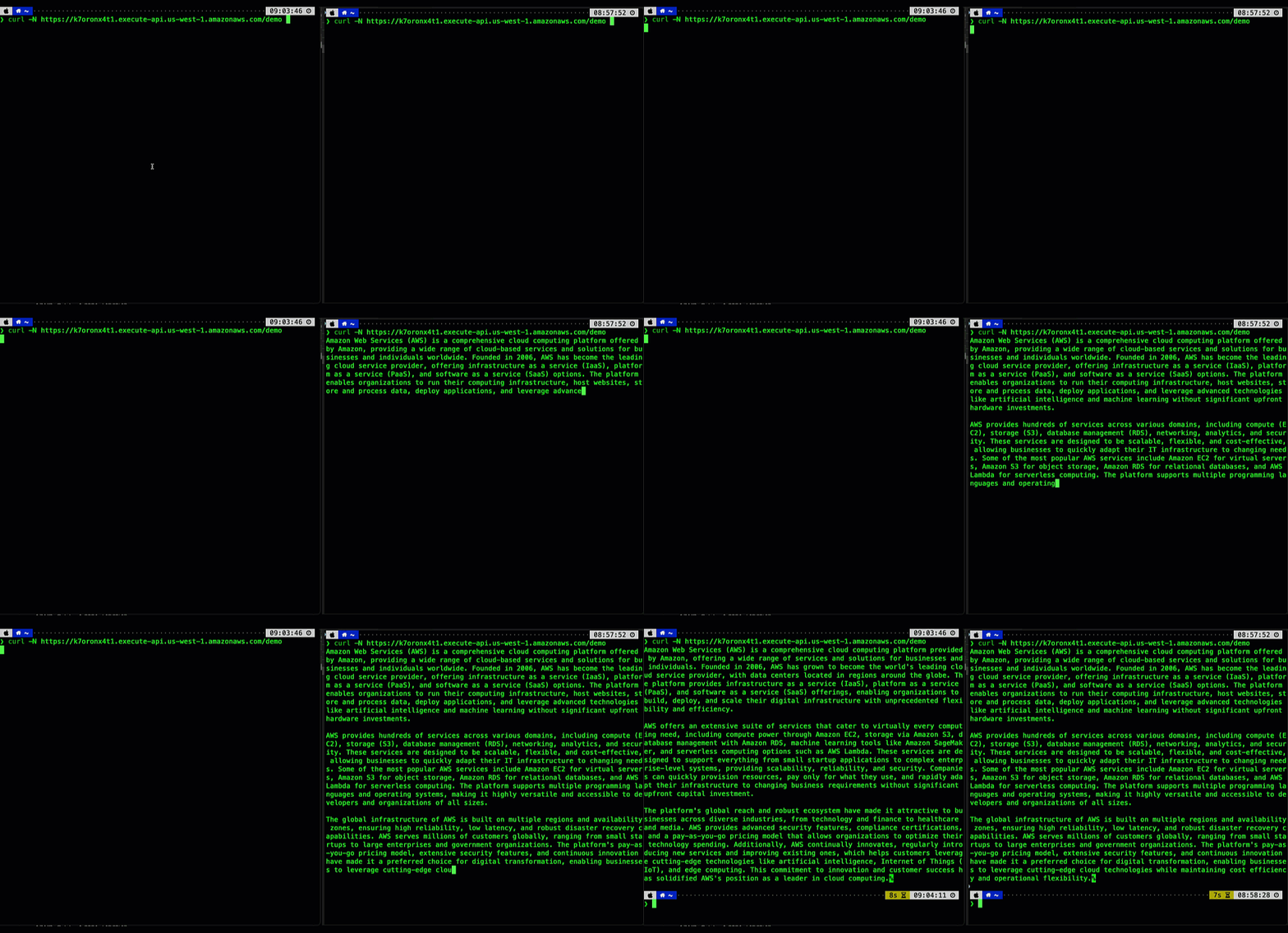
The following animation illustrates this significant user experience improvement. The prompt on the left is processed using a non-streaming response with user having to wait for several seconds to receive the result. The prompt on the right is using the new API Gateway response streaming, significantly reducing TTFB and improving user experience.

Figure 1. Comparing user experience before (left) and after (right) enabling API Gateway response streaming when returning a response from a Bedrock foundational model.

Your users can now see AI responses appear in real-time, word by word, just like watching someone type. This immediate feedback makes your applications feel more responsive and engaging, keeping users connected throughout the interaction. In addition, you don’t have to worry about response size limits or implement complex workarounds – the streaming happens automatically and efficiently, letting you focus on building great user experiences rather than managing infrastructure constraints.

Understanding response steaming

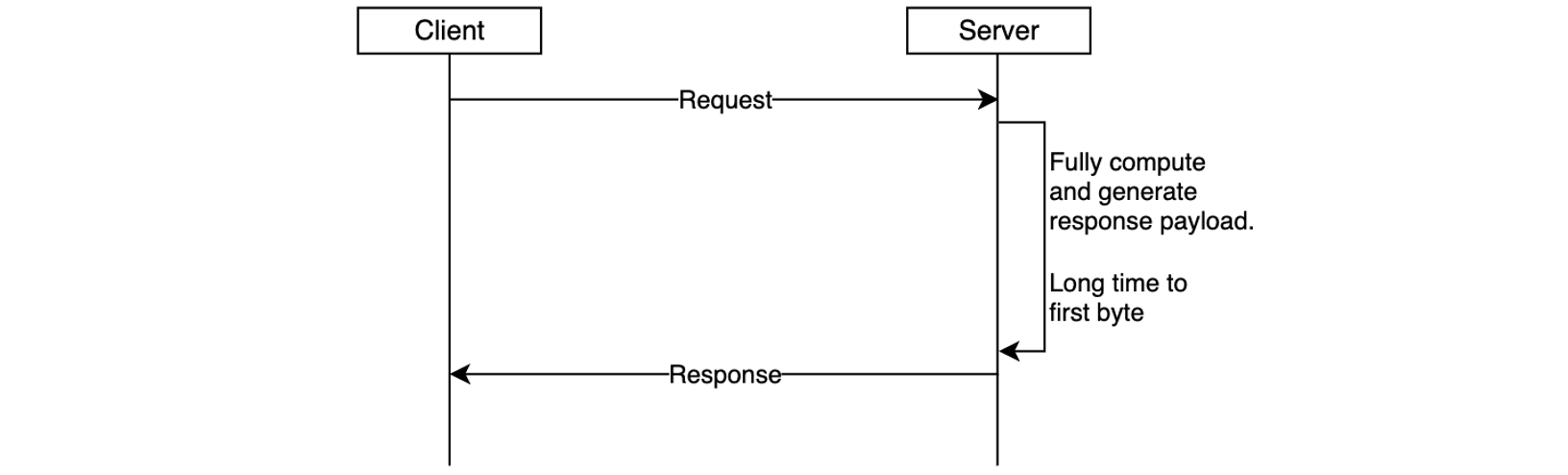
In the traditional request-response model, responses must be fully computed before being sent to the client. This can negatively impact user experience – the client must wait for the complete response to be generated on the server-side and transmitted over-the-wire. This is especially pronounced in interactive, latency-sensitive cloud applications such as AI agents, chatbots, virtual assistants, or music generators.

Figure 2. Response is returned to the client only after it’s been fully generated, increasing time-to-first-byte latency.

Another important scenario is returning larger response payloads, such as images, large documents, or datasets. In some cases, these payloads may exceed the 10 MB response size limit or default integration timeout limit of 29 seconds of API Gateway. Before the launch of response streaming, developers worked around these limitations by using pre-signed Amazon S3 URLs to download large responses or accepting lower RPS for an increase in timeout. While functional, these workarounds introduced additional latency and architectural complexity.

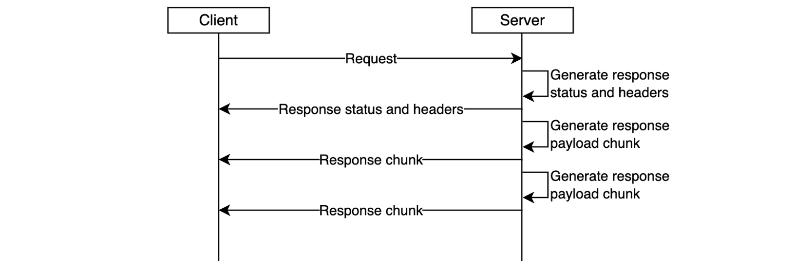
With response streaming support you can address these challenges. You can now update your REST APIs to return streamed responses, significantly enhancing user experience, improving TTFB performance, supporting response payload sizes to exceed 10 MB, and serving requests that can take up to 15 minutes.

Figure 3. Response streaming reduces time-to-first-byte and improves user experience.

The response streaming capability is already delivering significant performance for organizations:

“Working closely with the AWS teams to enable response streaming was instrumental in advancing our roadmap to deliver the most performant storefront experiences for our largest customers at Salesforce Commerce Cloud. Our collaboration exceeded our Core Web Vital goals; we saw our Total Blocking Time metrics drop by over 98%, which will enable our customers to drive higher revenue and conversion rates.”, says Drew Lau, Senior Director of Product Management at Salesforce.

Response streaming is supported for any HTTP-proxy integration, AWS Lambda functions (using proxy integration mode), and private integrations. To get started, configure your API integration to stream the response from your backend, as described in the following sections, and redeploy your API for changes to take effect.

Getting started with response streaming

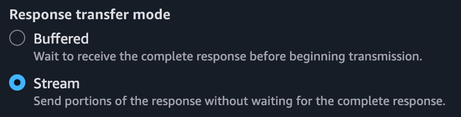
To enable response streaming for your REST APIs, update your integration configuration to set the response transfer mode to STREAM. This enables API Gateway to start streaming the response to the client as soon as response bytes become available. When using response streaming, you can configure request timeout up to 15 minutes. For best time to first byte user experience, AWS strongly recommends your backend integration also implements response streaming.

You can enable response streaming in several different ways, as illustrated in the following snippets:

Using the API Gateway console, when creating method integrations, select Stream for the Response transfer mode.

Figure 4. Enabling response streaming in API Gateway Console.

Setting response transfer mode using the Open API spec:

paths:
  /products:
    get:
      x-amazon-apigateway-integration:
        httpMethod: "GET"
        uri: "https://example.com"
        type: "http_proxy"
        timeoutInMillis: 300000
        responseTransferMode: "STREAM"

Setting response transfer mode using infrastructure-as-code (IaC) frameworks, such as AWS CloudFormation. Note the /response-streaming-invocations Uri fragment, it tells API Gateway to use the Lambda InvokeWithResponseStreaming endpoint:

MyProxyResourceMethod:
  Type: 'AWS::ApiGateway::Method'
  Properties:
    RestApiId: !Ref LambdaSimpleProxy
    ResourceId: !Ref ProxyResource
    HttpMethod: ANY
    Integration:
      Type: AWS_PROXY
      IntegrationHttpMethod: POST
      ResponseTransferMode: STREAM
      Uri: !Sub arn:aws:apigateway:${APIGW_REGION}:lambda:path/2021-11-
           15/functions/${FN_ARN}/response-streaming-invocations

Updating response transfer mode using the AWS CLI:

aws apigw update-integration \
   --rest-api-id a1b2c2 \
   --resource-id aaa111 \
   --http-method GET \
   --patch-operations "op='replace',path='/responseTransferMode',value=STREAM" \
   --region us-west-2

Using response streaming with Lambda functions

When using Lambda functions as a downstream integration endpoint, your Lambda functions must be streaming-enabled. The API Gateway uses the InvokeWithResponseStreaming API to invoke functions, as illustrated in the following diagram, and requires Lambda proxy integration. See the API Gateway documentation for additional guidance.

Figure 5. Using API Gateway response streaming with Lambda functions for interactive AI applications.

When you use response streaming with Lambda functions, API Gateway expects the handler response stream to contain the following components (in order):

  • JSON response metadata – Must be a valid JSON object and can only contain statusCode, headers, multiValueHeaders, and cookies fields (all optional). Metadata cannot be an empty string; at a minimum it must be an empty JSON object.
  • The 8-null-byte delimiter – Lambda adds this delimiter automatically when you use the built-in awslambda.HttpResponseStream.from() method, as illustrated below. When not using this method, you’re responsible for adding the delimiter yourself.
  • Response payload – Can be empty.

The following code snippet illustrates how you can return a streamed response from your Lambda functions so it will be compatible with API Gateway response streaming:

export const handler = awslambda.streamifyResponse(
   async (event, responseStream, context) => {

      const httpResponseMetadata = {
         statusCode: 200,
         headers: {
            'Content-Type': 'text/plain',
            'X-Custom-Header': 'some-value'
         }
      };

      responseStream = awslambda.HttpResponseStream.from(
         responseStream,
         httpResponseMetadata
      );

      responseStream.write('hello');
      await new Promise(r => setTimeout(r, 1000));
      responseStream.write(' world');
      await new Promise(r => setTimeout(r, 1000));
      responseStream.write('!!!');
      responseStream.end();
   }
);

Refer to the API Gateway documentation for further implementation guidelines.

Using response streaming with HTTP Proxy integrations

You can stream HTTP responses from your applications used as downstream integration endpoints, for example web servers running on Amazon Elastic Container Service (Amazon ECS) or Amazon Elastic Kubernetes Service (Amazon EKS). In this case, you must use HTTP_PROXY integration and specify the response transfer mode as STREAM (using the console, AWS CLI, or IaC). Redeploy your API after modifying it.

Figure 6. Using API Gateway response streaming with HTTP server applications.

Once API Gateway receives a streaming response from your application, it will wait until the HTTP headers block transfer is complete. Then, it will send to the client an HTTP response status code and headers, followed by the content from your application as it gets received by the API Gateway service. It will continue streaming response from your application to the client until the stream ends (up to 15 minutes).

Many popular API and web application development frameworks provide response streaming abstractions. The following code snippet illustrates how you can implement HTTP response streaming using FastAPI:

app = FastAPI()

async def stream_response():
   yield b"Hello "
   await asyncio.sleep(1)
   yield b"World "
   await asyncio.sleep(1)
   yield b"!"

@app.get("/")
async def main():
   return StreamingResponse(stream_response(), media_type="text/plain")

Adding real-time response streaming to your HTTP clients

Different HTTP clients have different ways to process streamed response fragments as they arrive. The following code snippet illustrates how to process a streamed response with a Node.js application:

const request = http.request(options, (response)=>{
   response.on('data', (chunk) => {
      console.log(chunk);
   });

   response.on('end', () => {
      console.log('Response complete’);
   });
});

request.end();

When using CURL, you can use the –no-buffer argument to print response fragments as they arrive.

curl --no-buffer {URL}

Sample code

Clone this sample project from GitHub to see API Gateway response streaming in action. Follow instructions in the README.md to provision the sample project in your AWS account.

Considerations

Before you enable response streaming, consider:

  • Response streaming is available for REST APIs and can be used with HTTP_PROXY integrations, Lambda integrations (in proxy mode), and private integrations.
  • You can use API Gateway response streaming with any endpoint type, such as Regional, Private, and Edge-optimized, with or without custom domain names.
  • When using response streaming, you can configure response timeouts up to 15 minutes, according to your scenario requirements.
  • All streaming responses from Regional or Private endpoints are subject to a 5-minute idle timeout. All streaming responses from edge-optimized endpoints are subject to a 30-second idle timeout.
  • Within each streaming response, the first 10MB of response payload is not subject to any bandwidth restrictions. Response payload data exceeding 10MB is restricted to 2MB/s.
  • Response streaming is compatible with API Gateway security capabilities such as authorizers, WAF, access controls, TLS/mTLS, request throttling, and access logging.
  • When processing streamed responses, the following features are not supported: response transformation with VTL, integration response caching, and content encoding.
  • Always protect your APIs against unauthorized access and other potential security threats by implementing proper authorization with Lambda Authorizers or Amazon Cognito User Pools. Read REST API protection documentation and API Gateway security documentation for additional details.

Observability

You can continue using existing observability capabilities, such as execution logs, access logs, AWS X-Ray integration, and Amazon CloudWatch metrics with API Gateway response streaming.

In addition to the existing access logs variables, the following new variables are available:

  • $content.integration.responseTransferMode – the response transfer mode of your integration. This can be either BUFFERED or STREAMED.
  • $context.integration.timeToAllHeaders – the time between when API Gateway establishes the integration connection to when it receives all integration response headers from the client.
  • $context.integration.timeToFirstContent – the time between when API Gateway establishes the integration connection to when it receives the first content bytes.

See API Gateway documentation for more information.

Pricing

With this new capability, you continue to pay the same API Invoke rates for streamed responses. Each 10MB of response data, rounded up to the nearest 10MB, is billed as a single request. See API Gateway pricing page for additional details.

Conclusion

The new response streaming capability for Amazon API Gateway enhances how you can build and deliver responsive APIs in the cloud. With immediate streaming of response data as it becomes available, you can significantly improve time-to-first-byte performance and overcome traditional payload size and timeout limitations. This is particularly valuable for AI-powered applications, file transfers, and interactive web experiences that demand real-time responsiveness.

To learn more about API Gateway response streaming see the service documentation.

To learn more about building Serverless architectures see Serverless Land.

Streamlined multi-tenant application development with tenant isolation mode in AWS Lambda

Post Syndicated from Donnie Prakoso original https://aws.amazon.com/blogs/aws/streamlined-multi-tenant-application-development-with-tenant-isolation-mode-in-aws-lambda/

Multi-tenant applications often require strict isolation when processing tenant-specific code or data. Examples include software-as-a-service (SaaS) platforms for workflow automation or code execution where customers need to ensure that execution environments used for individual tenants or end users remain completely separate from one another. Traditionally, developers have addressed these requirements by deploying separate Lambda functions for each tenant or implementing custom isolation logic within shared functions which increased architectural and operational complexity.

Today, AWS Lambda introduces a new tenant isolation mode that extends the existing isolation capabilities in Lambda. Lambda already provides isolation at the function level, and this new mode extends isolation to the individual tenant or end-user level within a single function. This built-in capability processes function invocations in separate execution environments for each tenant, enabling you to meet strict isolation requirements without additional implementation effort to manage tenant-specific resources within function code.

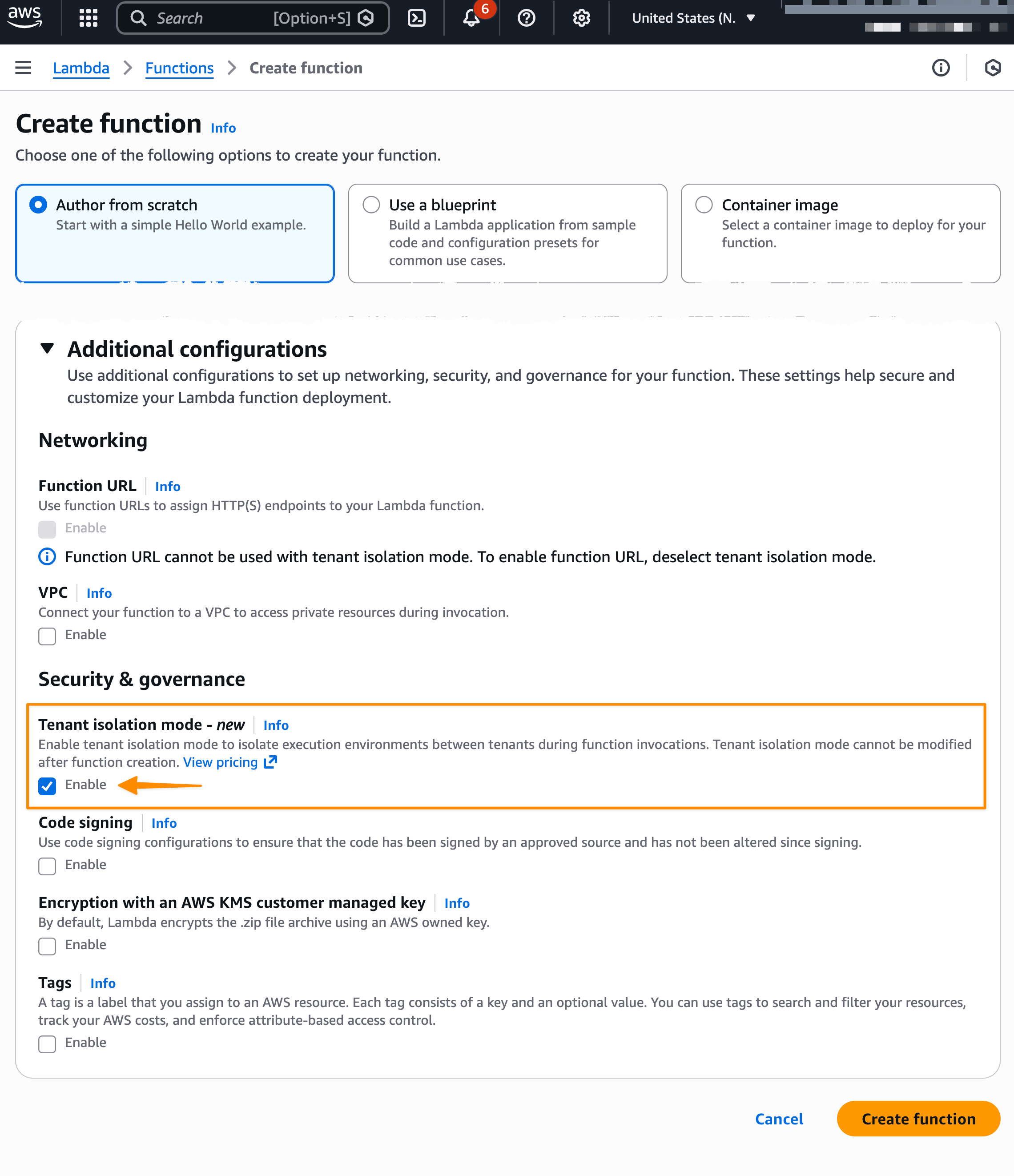
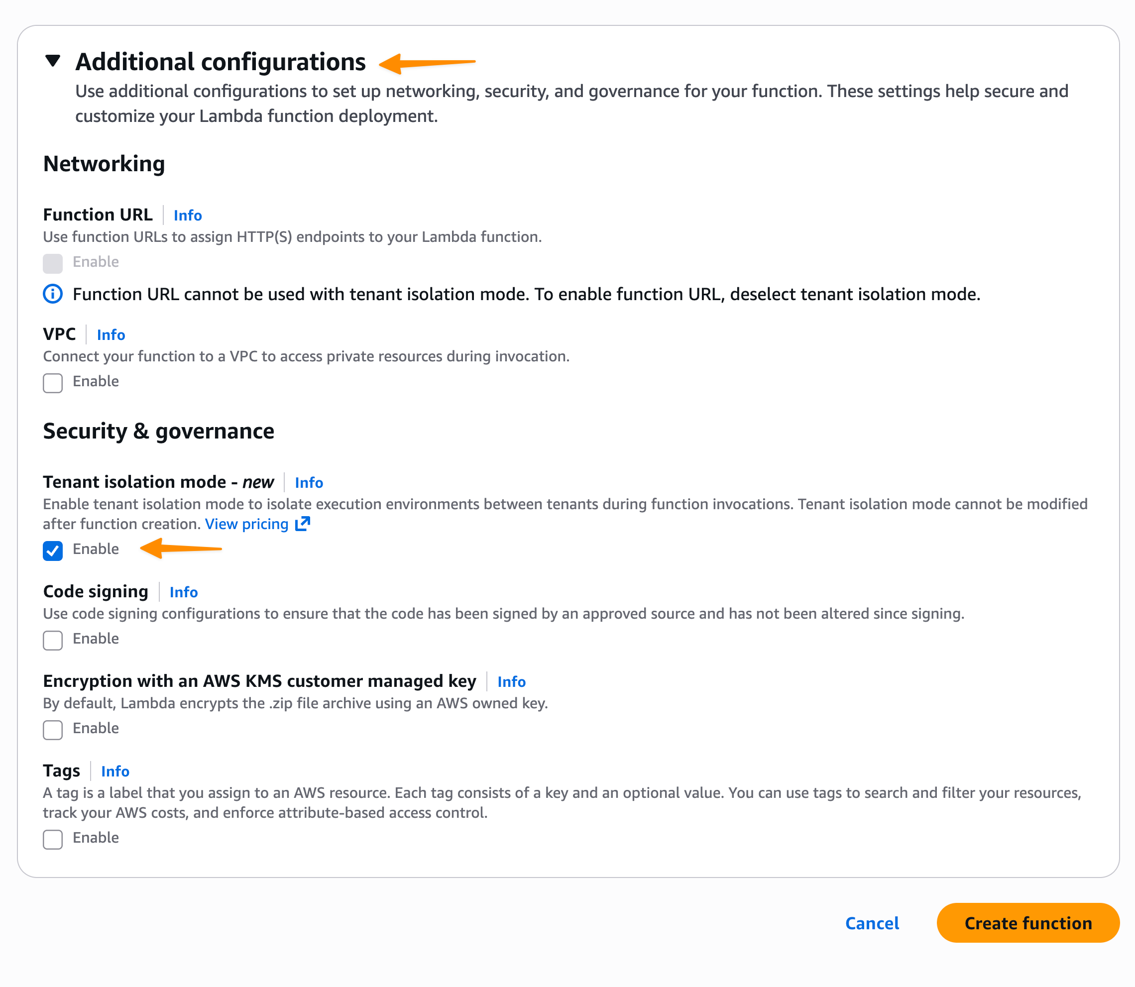
Here’s how you can enable tenant isolation mode in the AWS Lambda console:

When using the new tenant isolation capability, Lambda associates function execution environments with customer-specified tenant identifiers. This means that execution environments for a particular tenant aren’t used to serve invocation requests from other tenants invoking the same Lambda function.

The feature addresses strict security requirements for SaaS providers processing sensitive data or running untrusted tenant code. You maintain the pay-per-use and performance characteristics of AWS Lambda while gaining execution environment isolation. Additionally, this approach delivers the security benefits of per-tenant infrastructure without the operational overhead of managing dedicated Lambda functions for individual tenants, which can quickly grow as customers adopt your application.

Getting started with AWS Lambda tenant isolation
Let me walk you through how to configure and use tenant isolation for a multi-tenant application.

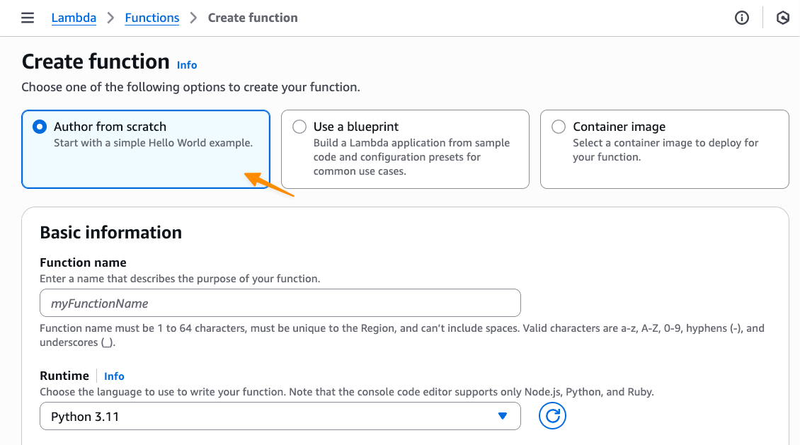
First, on the Create function page in the AWS Lambda console, I choose Author from scratch option.

Then, under Additional configurations, I select Enable under Tenant isolation mode. Note that, tenant isolation mode can only be set during function creation and can’t be modified for existing Lambda functions.

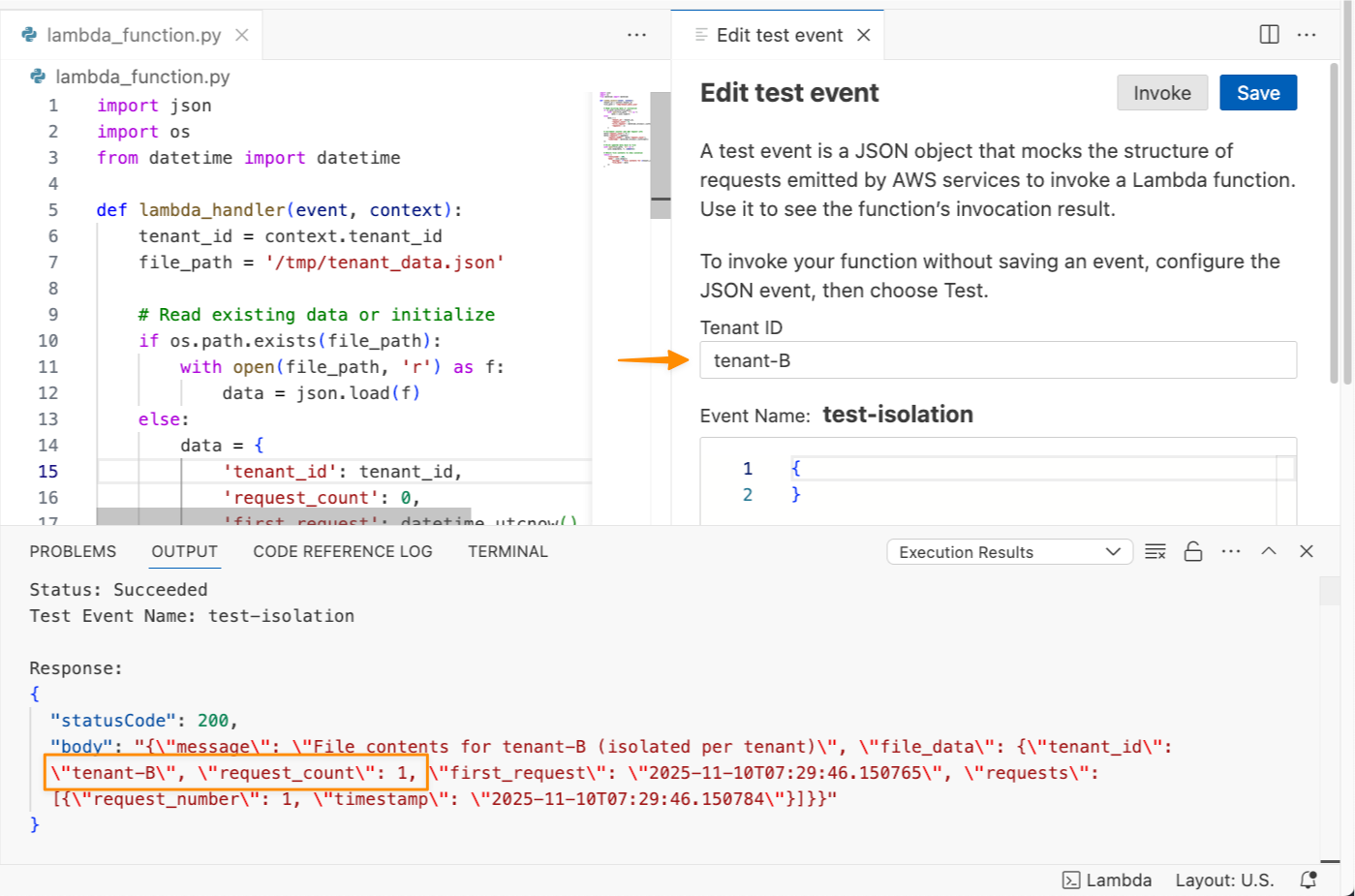
Next, I write Python code to demonstrate this capability. I can access the tenant identifier in my function code through the context object. Here’s the full Python code:

import json
import os
from datetime import datetime

def lambda_handler(event, context):
    tenant_id = context.tenant_id
    file_path = '/tmp/tenant_data.json'

    # Read existing data or initialize
    if os.path.exists(file_path):
        with open(file_path, 'r') as f:
            data = json.load(f)
    else:
        data = {
            'tenant_id': tenant_id,
            'request_count': 0,
            'first_request': datetime.utcnow().isoformat(),
            'requests': []
        }

    # Increment counter and add request info
    data['request_count'] += 1
    data['requests'].append({
        'request_number': data['request_count'],
        'timestamp': datetime.utcnow().isoformat()
    })

    # Write updated data back to file
    with open(file_path, 'w') as f:
        json.dump(data, f, indent=2)

    # Return file contents to show isolation
    return {
        'statusCode': 200,
        'body': json.dumps({
            'message': f'File contents for {tenant_id} (isolated per tenant)',
            'file_data': data
        })
    }

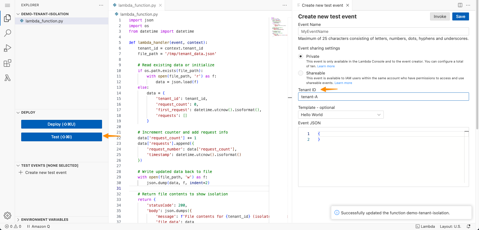
When I’m finished, I choose Deploy. Now, I need to test this capability by choosing Test. I can see on the Create new test event panel that there’s a new setting called Tenant ID.

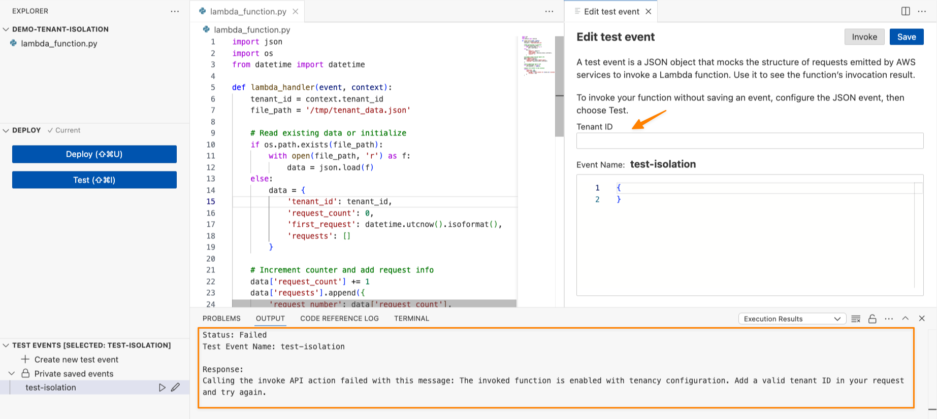
If I try to invoke this function without a tenant ID, I’ll get the following error “Add a valid tenant ID in your request and try again.”

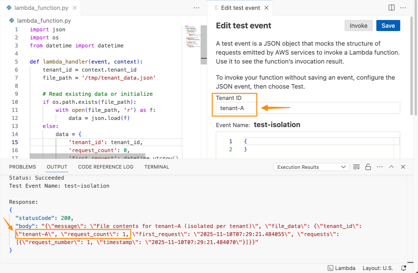
Let me try to test this function with a tenant ID called tenant-A.

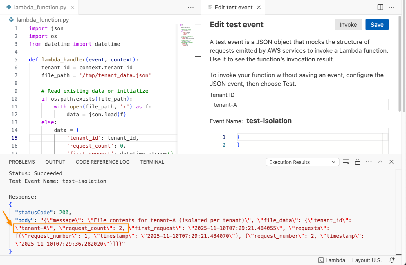
I can see the function ran successfully and returned request_count: 1. I’ll invoke this function again to get request_count: 2.

Now, let me try to test this function with a tenant ID called tenant-B.

The last invocation returned request_count: 1 because I never invoked this function with tenant-B. Each tenant’s invocations will use separate execution environments, isolating the cached data, global variables, and any files stored in /tmp.

This capability transforms how I approach multi-tenant serverless architecture. Instead of wrestling with complex isolation patterns or managing hundreds of tenant-specific Lambda functions, I let AWS Lambda automatically handle the isolation. This keeps tenant data isolated across tenants, giving me confidence in the security and separation of my multi-tenant application.

Additional things to know
Here’s a list of additional things you need to know:

  • Performance — Same-tenant invocations can still benefit from warm execution environment reuse for optimal performance.
  • Pricing — You’re charged when Lambda creates a new tenant-aware execution environment, with the price depending on the amount of memory you allocate to your function and the CPU architecture you use. For more details, view AWS Lambda pricing.
  • Availability — Available now in all commercial AWS Regions except Asia Pacific (New Zealand), AWS GovCloud (US), and China Regions.

This launch simplifies building multi-tenant applications on AWS Lambda, such as SaaS platforms for workflow automation or code execution. Learn more about how to configure tenant isolation for your next multi-tenant Lambda function in the AWS Lambda Developer Guide.

Happy building!
— Donnie

Python 3.14 runtime now available in AWS Lambda

Post Syndicated from Leandro Cavalcante Damascena original https://aws.amazon.com/blogs/compute/python-3-14-runtime-now-available-in-aws-lambda/

AWS Lambda now supports Python 3.14 as both a managed runtime and container base image. Python is a popular language for building serverless applications. Developers can now take advantage of new features and enhancements when creating serverless applications on Lambda.

You can develop Lambda functions in Python 3.14 using the AWS Management Console, AWS Command Line Interface (AWS CLI), AWS SDK for Python (Boto3), AWS Serverless Application Model (AWS SAM), AWS Cloud Development Kit (AWS CDK), and other infrastructure as code tools.

The Python 3.14 runtime supports Powertools for AWS Lambda (Python), a developer toolkit that helps you to implement serverless best practices. Powertools includes observability, batch processing, AWS Systems Manager Parameter Store integration, idempotency, feature flags, Amazon CloudWatch metrics, structured logging, and more.

Lambda@Edge allows you to use Python 3.14 to customize low-latency content delivered through Amazon CloudFront.

This blog post highlights notable Python language updates, Python Lambda runtime features and support, and how you can use the new Python 3.14 runtime in your serverless applications.

New Python features

Python 3.14 contains the following notable updates.

Template strings literal

Template strings introduce a new mechanism for custom string processing using the t prefix instead of f for f-strings. Unlike f-strings that return a simple string, t-strings return an object representing both static and interpolated parts.

Evaluation of type annotations

With the implementation of PEP 649, Python 3.14 defers type annotation evaluation until required. This reduces import time overhead and resolves forward reference issues.

Improved Error Messages

The interpreter now provides helpful suggestions when it detects typos in Python keywords. These include incorrect control flow structures, misused conditional expressions, string syntax errors, incompatible type usage in dicts/sets, and context manager protocol mismatches.

whille :

Traceback (most recent call last):
  File "<stdin>", line 1
    whille :
    ^^^^^^
SyntaxError: invalid syntax. Did you mean 'while'?

Standard library

The standard library includes a new compression.zstd module that provides native support for zstandard compression, offering better compression ratios and faster decompression compared to existing algorithms.

Python 3.14 also includes improved error messages and enhanced asyncio introspection capabilities.

Lambda runtime changes

The Lambda Python runtime contains the following changes.

Python 3.14 features that are not available

Python 3.14 includes some features that are not enabled for the Lambda managed runtime or base images. These features must be enabled when the Python runtime is compiled and cannot be enabled via an execution-time flag. The just-in-time (JIT) compiler is not available in the Lambda runtime because it’s still in an experimental phase. Free-threaded mode, running Python without the global interpreter lock, is supported in Python 3.14, but it is not enabled in the Lambda runtime due to potential performance impact. To use these features in Lambda, you can deploy your own Python runtime build with these features enabled, using a container image or custom runtime.

Amazon Linux 2023

As with the Python 3.12 and Python 3.13 runtimes, the Python 3.14 runtime is based on the provided.al2023 runtime, which is based on the Amazon Linux 2023 minimal container image. The Amazon Linux 2023 minimal image uses microdnf as a package manager, symlinked as dnf. This replaces the yum package manager used in Python 3.11 and earlier AL2-based images. If you deploy your Lambda functions as container images, you must update your Dockerfiles to use dnf instead of yum when upgrading to the Python 3.14 base image from Python 3.11 or earlier base images.

Learn more about the provided.al2023 runtime in the blog post Introducing the Amazon Linux 2023 runtime for AWS Lambda and the Amazon Linux 2023 launch blog post.

Using Python 3.14 in Lambda

You can use Python 3.14 for your Lambda functions in the AWS Management Console, an AWS Lambda container image, or the AWS Cloud Development Kit (AWS CDK).

AWS Management Console

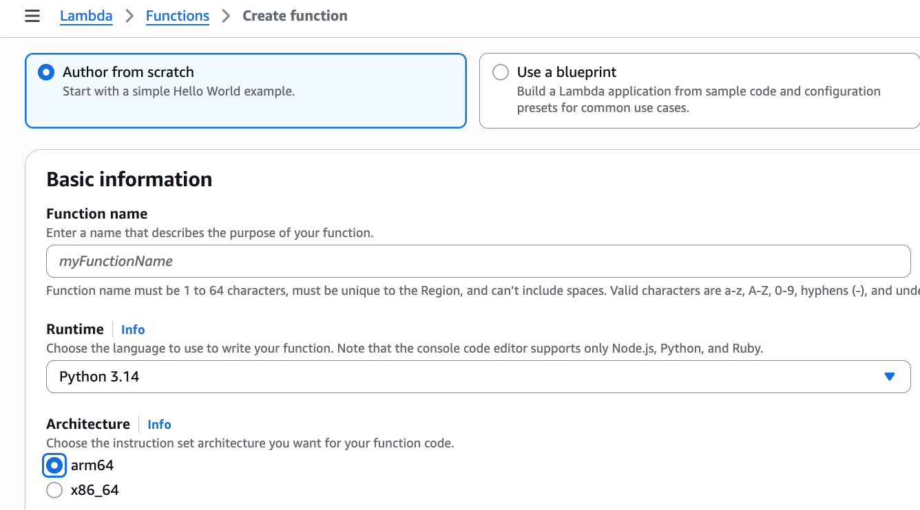
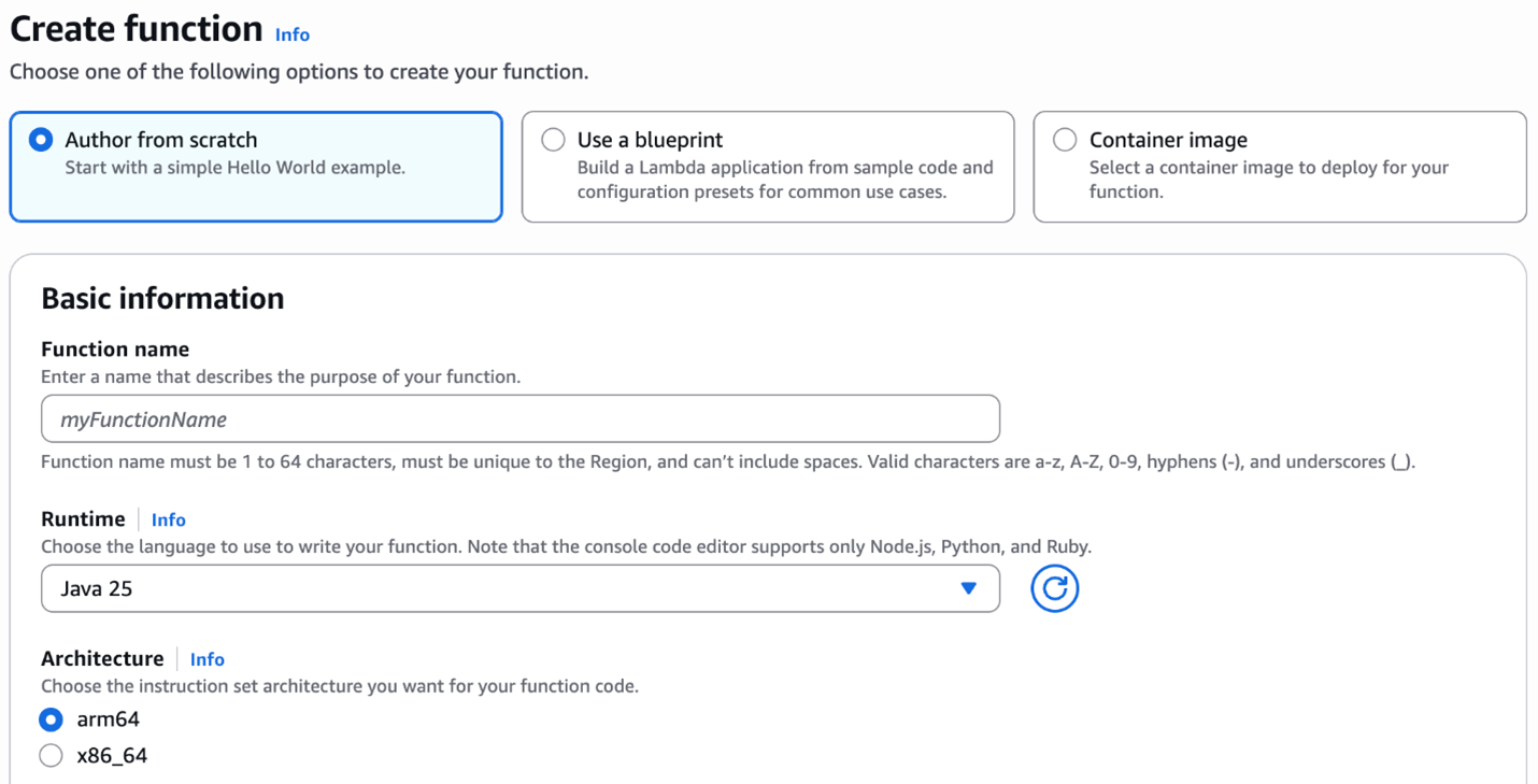
To use the Python 3.14 runtime to develop your Lambda functions, specify a runtime parameter value of Python 3.14 when creating or updating a function. On the Create Function page of the AWS Lambda console, Python 3.14 is available in the Runtime dropdown menu.

Create function page of the AWS Lambda console

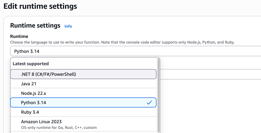
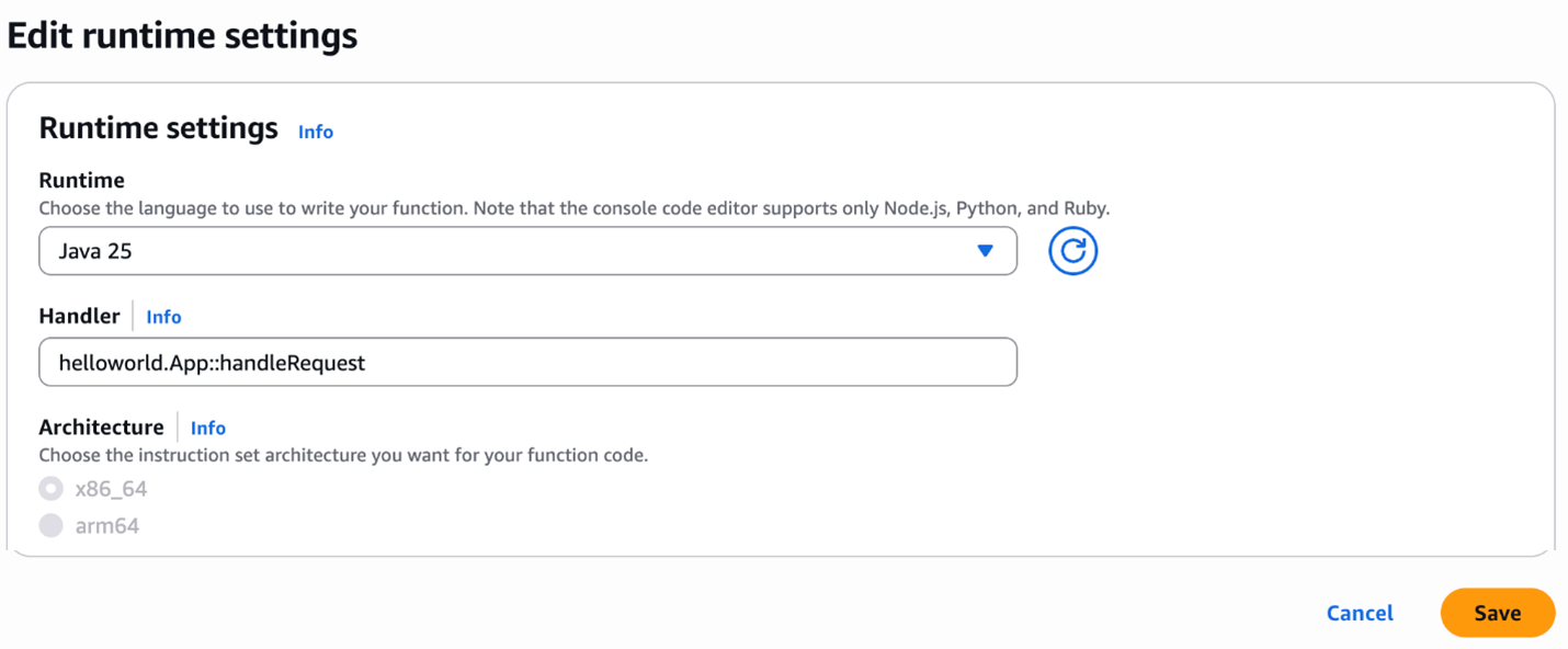
To update an existing Lambda function to Python 3.14, navigate to the function in the Lambda console and choose Edit in the Runtime settings panel. The new version of Python is available in the Runtime dropdown menu.

The runtime dropdown menu

Upgrading a function to Python 3.14

To upgrade a function to Python 3.14, check your code and dependencies for compatibility with Python 3.14, run tests, and update as necessary. Consider using generative AI coding assistants like Amazon Q Developer, Amazon Q Developer for CLI, or Kiro to help with upgrades.

AWS Lambda container image

Change the Python base image version by modifying the FROM statement in your Dockerfile:

FROM public.ecr.aws/lambda/python:3.14
# Copy function code
COPY lambda_handler.py ${LAMBDA_TASK_ROOT}

AWS Serverless Application Model (AWS SAM)

In AWS SAM set the Runtime attribute to python3.14 to use this version.

AWSTemplateFormatVersion: '2010-09-09'
Transform: AWS::Serverless-2016-10-31
Description: Simple Lambda Function
  MyFunction:
    Type: AWS::Serverless::Function
    Properties:
      Description: My Python Lambda Function
      CodeUri: my_function/
      Handler: lambda_function.lambda_handler
      Runtime: python3.14

AWS SAM supports generating this template with Python 3.14 for new serverless applications using the sam init command. Refer to the AWS SAM documentation.

AWS Cloud Development Kit

In the AWS CDK, set the runtime attribute to lambda.Runtime.PYTHON_3_14 to use this version.

In Python CDK:

from constructs import Construct
from aws_cdk import ( App, Stack, aws_lambda as _lambda )
class SampleLambdaStack(Stack):
    def __init__(self, scope: Construct, id: str, **kwargs) -> None:
        super().__init__(scope, id, **kwargs)

        base_lambda = _lambda.Function(self, 'python314LambdaFunction',
                                       handler='lambda_handler.handler',
                                    runtime=_lambda.Runtime.PYTHON_3_14,
                                 code=_lambda.Code.from_asset('lambda'))

In TypeScript CDK:

import * as cdk from 'aws-cdk-lib';
import * as lambda from 'aws-cdk-lib/aws-lambda'
import * as path from 'path';
import { Construct } from 'constructs';
export class SampleLambdaStack extends cdk.Stack {
  constructor(scope: Construct, id: string, props?: cdk.StackProps) {
    super(scope, id, props);
    // The code that defines your stack goes here
    // The python3.14 enabled Lambda Function
    const lambdaFunction = new lambda.Function(this, 'python314LambdaFunction', {
      runtime: lambda.Runtime.PYTHON_3_14,
      memorySize: 512,
      code: lambda.Code.fromAsset(path.join(__dirname, '/../lambda')),
      handler: 'lambda_handler.handler'
    })
  }
}

Serverless Land Patterns AWS Top Picks for Python, now use Python 3.14.

Performance considerations

At launch, new Lambda runtimes receive less usage than existing established runtimes. This can result in longer cold start times due to reduced cache residency within internal Lambda sub-systems. Cold start times typically improve in the weeks following launch as usage increases. As a result, AWS recommends not drawing conclusions from side-by-side performance comparisons with other Lambda runtimes until the performance has stabilized. Since performance is highly dependent on workload, customers with performance-sensitive workloads should conduct their own testing instead of relying on generic test benchmarks.

Conclusion

Lambda now supports Python 3.14 as a managed language runtime to help developers build more efficient, powerful, and scalable serverless applications. Python 3.14 language additions include data model improvements, typing changes, and updates to the standard library. The Lambda managed runtime does not include the option to disable the global interpreter lock (GIL) or use the experimental JIT compiler.

You can build and deploy functions using Python 3.14 using the AWS Management Console, AWS CLI, AWS SDK, AWS SAM, AWS CDK, or your choice of infrastructure as code tool. You can also use the Python 3.14 container base image if you prefer to build and deploy your functions using container images.

Try the Python 3.14 runtime in Lambda today and experience the benefits of this updated language version.

To find more Python examples, use the Serverless Patterns Collection. For more serverless learning resources, visit Serverless Land.

Building serverless applications with Rust on AWS Lambda

Post Syndicated from Julian Wood original https://aws.amazon.com/blogs/compute/building-serverless-applications-with-rust-on-aws-lambda/

Today, AWS Lambda is promoting Rust support from Experimental to Generally Available. This means you can now use Rust to build business-critical serverless applications, backed by AWS Support and the Lambda availability SLA.

Rust is a popular programming language due to its combination of high performance, memory safety, and developer experience. It offers speed and memory utilization efficiency comparable with C++, together with the reliability normally associated with higher-level languages.

This post shows you how to build and deploy Rust-based Lambda functions using Cargo Lambda, a third-party open source tool for working with Lambda functions in Rust. We’ll also cover how to deploy your functions using the Cargo Lambda AWS Cloud Development Kit (AWS CDK) construct.

Prerequisites

Before you begin, make sure you have:

  • An AWS account with appropriate permissions.
  • The AWS Command Line Interface (AWS CLI) configured with your credentials
  • Rust installed on your development machine (version 1.70 or later)
  • Node.js 20 or later (for AWS CDK deployment)
  • AWS CDK installed: npm install -g aws-cdk

Solution overview

This post takes you through the following steps:

  1. Install and configure Cargo Lambda.
  2. Create and deploy a basic HTTP Lambda function using Cargo Lambda.
  3. Build a complete serverless API using AWS CDK with Rust Lambda functions.

Install and configure Cargo Lambda

Cargo is the package manager and build system for Rust. Cargo Lambda is a third-party open source extension to the cargo command-line tool that simplifies building and deploying Rust Lambda functions.

To install Cargo Lambda on Linux systems, run:

curl -fsSL https://cargo-lambda.info/install.sh | sh

For additional installation options, see the Cargo Lambda installation documentation.

Creating your first Rust Lambda function

Create an HTTP-based Lambda function:

cargo lambda new hi_api

When prompted for Is this function an HTTP function?, enter y.

cd hi_api

This creates a project with the following structure:

├── Cargo.toml
├── README.md
└── src
    ├── http_handler.rs
    └── main.rs

The project includes:

  • main.rs – The function entry point where you configure dependencies and shared state
  • http_handler.rs – The primary function logic

The main.rs file contains the following code:

use lambda_http::{run, service_fn, tracing, Error};
mod http_handler;
use http_handler::function_handler;
#[tokio::main]
async fn main() -> Result<(), Error> {
tracing::init_default_subscriber();
run(service_fn(function_handler)).await
}

The key part of the main.rs file is run(service_fn(function_handler)).await. The run function is part of the http_lambda crate and starts the Lambda Rust runtime interface client (RIC), which actively polls for events from the Lambda Runtime API. The function_handler is the function that is defined in the http_handler.rs file. When the Runtime API returns the invoke event, the RIC calls the function_handler from http_handler.rs:

use lambda_http::{Body, Error, Request, RequestExt, Response};
pub(crate) async fn function_handler(event: Request) -> Result<Response, Error> {
// Extract some useful information from the request
let who = event
.query_string_parameters_ref()
.and_then(|params| params.first("name"))
.unwrap_or("world");
let message = format!("Hello {who}, this is an AWS Lambda HTTP request");
// Return something that implements IntoResponse.
// It will be serialized to the right response event automatically by the runtime

let resp = Response::builder()
    .status(200)
    .header("content-type", "text/html")
    .body(message.into())
    .map_err(Box::new)?;
Ok(resp)

}

The function_handler function signature includes a variable event of type Request. The event contents depend on the service triggering the function. For example, it may contain HTTP request information such as path parameters if the request is coming via HTTP, or even an array of Amazon Kinesis stream records.

For non-HTTP functions, events can be strongly typed. Additionally, you can accept any structure as input as long as it implements serde::Serialize and serde::Deserialize.

The example parses query parameters and looks for the first parameter that has the name name.

The lambda_http crate provides an idiomatic way to return a response, using a builder pattern. The function returns a response as a Result with an Ok() which is what the run function in main.rs expects.

Logging

The main.rs file includes the following line by default:

tracing::init_default_subscriber();

The Rust Lambda runtime integrates natively with Tracing libraries for logging and tracing, and supports JSON structured logging. When setting this line and the RUST_LOG environment variable, Lambda sends logs to Amazon CloudWatch. By default, the INFO log level is enabled.

To write logs, use the tracing crate and send events using the following syntax:

tracing::info("This is a log entry");

Building

To build the Lambda function, use cargo lambda build. When compiling the Lambda function, the AWS Lambda Runtime is built into your binary. The compiled binary file is called bootstrap. It is packaged in the function artifact .zip file and visible as a file in the AWS Lambda console.

When Lambda executes this binary, it starts an infinite loop (the Run function). This polls the Lambda Runtime API to receive the invoke request and then calls your handler, the function_handler function.

The Lambda runtime execution environment

Your function code runs and then sends the function response back to the Lambda Runtime API, which forwards it onto the caller.

Testing

Before deploying the function, you can debug/test the function locally using cargo lambda.

cargo lambda watch sets up an environment that emulates the Lambda execution environment. This allows you to send requests to the Lambda function and see the results.

To send invocation requests, you can use either cargo lambda or send a curl request to the Lambda emulator.

To use cargo lambda, run the following, replace <lambda-function-name> with hi_api for this example

cargo lambda invoke <lambda-function-name> --data-example apigw-request

You can use any of the built-in example payloads with the --data-example parameter. Use --data-ascii <payload> to provide your own payload.

To invoke the function using curl, pass the JSON format payload to the local emulator’s address:

curl -v -X POST \
  'http://127.0.0.1:9000/lambda-url/<lambda-function-name>/' \
  -H 'content-type: application/json' \
  -d '{ "command": "hi" }'

Deploying with Cargo Lambda

Once you have built the function using cargo lambda build, you can deploy it to your AWS account.

To deploy your function:

cargo lambda deploy

Once the Lambda function is deployed, you can test it remotely. cargo lambda invoke tests the remote Lambda function using a payload stored in a .json file:

cargo lambda invoke --remote hi_api --data-file <event file>

Infrastructure-as-Code with AWS CDK

You can create a serverless API in front of this Rust Lambda function using Amazon API Gateway. This example uses the AWS CDK. This example does not have authentication configured for the API Gateway endpoint as it is a sample. The AWS best practice is to implement relevant security controls where necessary.

  1. First, create a new CDK project:
    mkdir rusty_cdk
    cd rusty_cdk
    cdk init --language=typescript

    The easiest way to deploy a Rust Lambda function using the AWS CDK is to use the cargo lambda CDK Construct. This comes with everything required to run Rust Lambda functions on AWS. It is part of the cargo lambda project.

  2. Install the Cargo Lambda CDK construct:
    npm i cargo-lambda-cdk

  3. Create a new HTTP Lambda function in your project:
    mkdir lambda
    cd lambda
    cargo lambda new helloRust

    When prompted for Is this function an HTTP function?, enter y.

  4. Update your CDK stack lib/rusty_cdk-stack.ts to include both the Lambda function and API Gateway.
    import * as cdk from 'aws-cdk-lib';
    import { HttpApi } from 'aws-cdk-lib/aws-apigatewayv2';
    import { HttpLambdaIntegration } from 'aws-cdk-lib/aws-apigatewayv2-integrations';
    import { HttpMethod } from 'aws-cdk-lib/aws-events';
    import { RustFunction } from 'cargo-lambda-cdk';
    import { Construct } from 'constructs';
    export class RustyCdkStack extends cdk.Stack {
      constructor(scope: Construct, id: string, props?: cdk.StackProps) {
        super(scope, id, props);
        const helloRust = new RustFunction(this, 'helloRust',{
          manifestPath: './lambda/helloRust',
          runtime: 'provided.al2023',
          timeout: cdk.Duration.seconds(30),
        });
    
        const api = new HttpApi(this, 'rustyApi');
        const helloInteg = new HttpLambdaIntegration('helloInteg', helloRust);
    
        api.addRoutes({
          path: '/hello',
          methods: [HttpMethod.GET],
          integration: helloInteg,
        })
        new cdk.CfnOutput(this, 'apiUrl',{
          description: 'The URL of the API Gateway',
          value: `https://${api.apiId}.execute-api.${this.region}.amazonaws.com`,
        })
      }
    }

  5. Bootstrap your AWS account and AWS Region for the AWS CDK:
    cdk bootstrap

  6. Deploy your stack:
    cdk deploy

Testing the API

To test your deployed API using the URL provided in the AWS CDK output:

curl https://<YOUR_API_URL>/hello

Clean up

To avoid ongoing charges, remove the deployed resources:

cdk destroy

Conclusion

AWS Lambda support for Rust is now Generally Available to build high-performance, memory-efficient serverless applications. Cargo Lambda is a third-party extension to the Rust cargo CLI which simplifies the experience of developing, testing, and deploying Rust applications to Lambda.

To learn more about building serverless applications with Rust:

To find more Rust code examples, use the Serverless Patterns Collection. For more serverless learning resources, visit Serverless Land.

AWS Lambda now supports Java 25

Post Syndicated from Lefteris Karageorgiou original https://aws.amazon.com/blogs/compute/aws-lambda-now-supports-java-25/

You can now develop AWS Lambda functions using Java 25 either as a managed runtime or using the container base image. Java 25 support for Lambda is based on the Amazon Corretto distribution of OpenJDK and is now generally available.

Java 25 comes with new language features for developers, including primitive types in patterns, module import declarations, and flexible constructor bodies, as well as generational support to the Shenandoah garbage collector. There are Lambda runtime changes to optimize cold starts by using the new Java Ahead-of-Time (AOT) caches feature. This release also includes updates to the default tiered compilation for SnapStart and Provisioned Concurrency, and removes the Log4Shell patch. With this release, Java developers can take advantage of these new features and enhancements when creating serverless applications on Lambda.

You can develop Java 25 Lambda functions using the AWS Management Console, AWS Command Line Interface (AWS CLI), AWS SDK for JavaScript, AWS Serverless Application Model (AWS SAM), AWS Cloud Development Kit (AWS CDK), and other infrastructure as code tools. You can also use Java 25 with Powertools for AWS Lambda (Java), a developer toolkit to implement serverless best practices and increase developer velocity. Powertools for AWS Lambda includes libraries to support common tasks such as observability, AWS Systems Manager Parameter Store integration, idempotency, batch processing, and more.

This blog post highlights notable Java language features, Java Lambda runtime updates, and how you can use the new Java 25 runtime in your serverless applications.

Java 25 language features

Java 25 introduces several language features to enhance developer productivity. There is a new feature that allows statements to appear before an explicit constructor invocation. You can now write code in the constructors without having to invoke super(…) or this(…) as the first statement. In the following example, the Employee class has a constructor which validates the input first and then invokes super(...):


class Person {
    int age;

    Person(int age) {
        if (age < 0)
            throw new IllegalArgumentException("Age cannot be negative");

        this.age = age;
    }
}

class Employee extends Person {
    String name;

    Employee(String name, int age) {
        // This is now allowed - code before super()
        if (age < 18 || age > 67)
            throw new IllegalArgumentException(...);

        super(age);
        this.name = name;
    }
}

Java 25 supports pattern matching that can handle primitive types in switch and instanceof statements. Previously, pattern matching was limited to reference types (Objects). For example, you can now perform pattern matching with int values, not just Integer objects:

void primitivePatternMatching(Object obj) {
    if (obj instanceof int i) {
        System.out.println("This is an int: " + i);
    }
}

Module import declarations simplifies working with. Instead of writing multiple individual package imports from the same module, you can use the import module syntax to bring publicly exported types into scope. This reduces boilerplate code and makes it easier to work with modular applications. Previously if you used the java.net.http module, you had to import multiple classes with individual import statements:

import java.net.URI;
import java.net.http.HttpClient;
import java.net.http.HttpRequest;

public class HttpClientExample {
    public void makeRequest() {
        HttpClient client = HttpClient.newHttpClient();
        HttpRequest request = HttpRequest.newBuilder()
            .uri(URI.create("https://api.example.com"))
            .build();
        // ... rest of implementation
    }
}

Now you can import the whole java.net.http module:

import module java.net.http;

public class HttpClientExample {
    public void makeRequest() {
        HttpClient client = HttpClient.newHttpClient();
        HttpRequest request = HttpRequest.newBuilder()
            .uri(URI.create("https://api.example.com"))
            .build();
        // Exported types from java.net.http module are now available
    }
}

Garbage collection

The generational mode of the Shenandoah garbage collector changes from an experimental feature in Java 24 to an optional product feature. Shenandoah is the low pause time garbage collector that reduces pause times by performing more garbage collection work concurrently with the running Java program. Shenandoah does the bulk of GC work concurrently, including the concurrent compaction, which means its pause times are no longer directly proportional to the size of the heap. The generational mode of Shenandoah improves sustainable throughput, load-spike resilience, and memory utilization.

To use the generational model of Shenandoah in Lambda, set JAVA_TOOL_OPTIONS to -XX:+UseShenandoahGC -XX:ShenandoahGCMode=generational.

Lambda runtime updates

The Java 25 runtime includes several performance optimizations, tuned to optimize cold and warm start performance for a broad range of customer workloads. Cold start refers to the initialization delay that occurs when Lambda prepares a new execution environment for a function that hasn’t been invoked recently, or to process an incoming invoke when all existing execution environments are in use. Warm start refers to invokes that are allocated to a previously initialized execution environment.

Ahead-of-Time (AOT) caches

Starting with Java 25, AWS Lambda replaces the traditional Class Data Sharing (CDS) with ahead-of-time (AOT) caches. This is an advanced optimization feature from Project Leyden that is designed to improve application startup times and reduce memory footprint. Lambda’s benchmarking results show that AOT caches deliver faster cold start performance compared to CDS.

AOT caches are enabled by default to provide performance benefits. Since you cannot use both AOT caches and CDS, if you enable CDS in your Lambda function, then Lambda disables AOT caches. If you use your own custom AOT caches in the Java 25 managed runtime, then the caches may be invalidated when Lambda updates the Java runtime during routine patching. AWS strongly suggests that you don’t use custom AOT caches with managed runtimes.

If you deploy Java 25 functions using container images, you can either implement your own AOT caches or continue using CDS. Since container images are immutable, the issue of AOT caches being invalidated following automatic runtime patching does not arise. To enable AOT caches, pass the flag -XX:AOTCache=/path/to/aot/cache/file via the JAVA_TOOL_OPTIONS environment variable. To enable CDS, pass the flag -Xshare:on -XX:SharedArchiveFile=/var/lang/lib/server/runtime.jsa.

Tiered compilation

Java’s tiered compilation is a just-in-time (JIT) optimization strategy that employs multiple compiler tiers to enhance the performance of frequently executed code progressively using runtime profiling data. Since Java 17, AWS Lambda has modified the default JVM behavior by stopping compilation at the C1 tier (client compiler). This minimizes cold start times for function invocations for most functions, although for compute-intensive functions with a long duration, customers can benefit from tuning tiered compilation to their workload. Starting with Java 25, Lambda no longer stops tiered compilation at C1 for SnapStart and Provisioned Concurrency. This improves performance in these cases without incurring a cold start penalty since tiered compilation occurs outside of the invoke path in these cases.

Priming

Priming is another technique to optimize performance for functions using either SnapStart or Provisioned Concurrency. This involves preloading dependencies, initializing resources, and executing code paths during function initialization. This front-loads work and triggers JIT compilation before taking the SnapStart snapshot, or when Provisioned Concurrency execution environments are pre-provisioned. The result is faster code execution when these execution environments are used for a function warm invoke. For detailed guidance on implementing priming strategies, see the Optimizing cold start performance of AWS Lambda using advanced priming strategies with SnapStart blog post.

Log4j patch for Log4Shell

Log4j is a widely used open source logging library maintained by the Apache Software Foundation. In November 2021, Log4j reported Log4Shell, a zero-day vulnerability involving arbitrary code execution. The Lambda team responded by deploying an emergency patch across all Java runtimes to protect customers from potential exploitation. However, this emergency patch introduced a performance overhead during cold starts. The vulnerability was permanently resolved in Log4j version 2.17.0 in December 2021. Consequently, AWS has removed this patch from the Java 25 runtime to restore optimal performance. You must verify you are using Log4j version 2.17.0 or later.

Lambda runtimes for Java 8, 11, 17, and 21 continue to enable the emergency patch by default. Customers who are using Log4j version 2.17.0 or higher with these runtimes can disable this patch, improving cold start performance. To disable the patch, set the AWS_LAMBDA_DISABLE_CVE_2021_44228_PROTECTION environment variable to true.

Additional performance considerations

At launch, new Lambda runtimes receive less usage than existing, established runtimes. This can result in longer cold start times due to reduced cache residency within internal Lambda sub-systems. Cold start times typically improve in the weeks following launch as usage increases. As a result, AWS recommends not drawing conclusions from side-by-side performance comparisons with other Lambda runtimes until the performance has stabilized.

Since performance is highly dependent on workload, customers with performance-sensitive workloads should conduct their own testing instead of relying on generic test benchmarks. To maximize performance, your workload may benefit from additional workload-specific performance tuning.

Using Java 25 in AWS Lambda

You can use Java 25 for your Lambda functions in the AWS Management Console, an AWS Lambda container image, AWS SAM, or the AWS CDK.

AWS Management Console

To use the Java 25 runtime to develop your Lambda functions, specify a runtime parameter value Java 25 when creating or updating a function. The Java 25 runtime version is now available in the Runtime dropdown menu on the Create function page in the AWS Lambda console:

Creating Java 25 function in the AWS Management Console
Creating Java 25 function in AWS Management Console

To update an existing Lambda function to Java 25, navigate to the function in the Lambda console, then choose Java 25 in the Runtime settings section. The new version is available in the Runtime dropdown menu:

Changing a function to Java 25

Changing a function to Java 25

AWS Lambda container image

Use the Java base image version with the java:25 tag by modifying the FROM statement in your Dockerfile.

Example Dockerfile:

FROM public.ecr.aws/lambda/java:25
# Copy function code and runtime dependencies from Maven layout
COPY target/classes ${LAMBDA_TASK_ROOT}
COPY target/dependency/* ${LAMBDA_TASK_ROOT}/lib/
# Set the CMD to your handler (could also be done as a parameter override outside of the Dockerfile)
CMD [ "com.example.myapp.App::handleRequest" ]

To build a container image for a Java Lambda function, refer to the AWS Lambda documentation.

AWS Serverless Application Model (AWS SAM)

In AWS SAM, set the Runtime attribute to java25 to use this version:

AWSTemplateFormatVersion: '2010-09-09'
Transform: AWS::Serverless-2016-10-31
Description: Simple Lambda Function

Resources:
  HelloWorldFunction:
    Type: AWS::Serverless::Function
    Properties:
      CodeUri: HelloWorldFunction
      Handler: helloworld.App::handleRequest
      Runtime: java25
      MemorySize: 1024

AWS SAM supports generating this template with Java 25 for new serverless applications using the sam init command. Refer to the AWS SAM documentation.

AWS Cloud Development Kit (AWS CDK)

In the AWS CDK, set the runtime attribute to Runtime.JAVA_25 to use this version.

import software.amazon.awscdk.core.Construct;
import software.amazon.awscdk.core.Stack;
import software.amazon.awscdk.core.StackProps;
import software.amazon.awscdk.services.lambda.Code;
import software.amazon.awscdk.services.lambda.Function;
import software.amazon.awscdk.services.lambda.Runtime;

public class InfrastructureStack extends Stack {

    public InfrastructureStack(final Construct parent, final String id, final StackProps props) {

        super(parent, id, props);

        Function.Builder.create(this, "HelloWorldFunction")
                .runtime(Runtime.JAVA_25)
                .code(Code.fromAsset("target/hello-world.jar"))
                .handler("helloworld.App::handleRequest")
                .memorySize(1024)
                .build();

        // rest of your CDK code
    }
} 

Conclusion

Lambda now supports Java 25 as a managed language runtime or with your own custom runtime. This release includes the latest Java 25 language features as well as performance enhancements optimized for Lambda workloads.

You can build and deploy functions using Java 25 using the AWS Management Console, AWS CLI, AWS SDK, AWS SAM, AWS CDK, or your choice of infrastructure as code tool. You can also use the Java container base image with the 25 tag if you prefer to build and deploy your functions using container images.

The Java 25 runtime helps developers build more efficient, powerful, and scalable serverless applications. Read about the Java programming model in the Lambda documentation to learn more about writing functions in Java 25.

To find more Java examples, use the Serverless Patterns Collection. For more serverless learning resources, visit Serverless Land.


AWS Lambda enhances event processing with provisioned mode for SQS event-source mapping

Post Syndicated from Micah Walter original https://aws.amazon.com/blogs/aws/aws-lambda-enhances-sqs-processing-with-new-provisioned-mode-3x-faster-scaling-16x-higher-capacity/

Today, we’re announcing the general availability of provisioned mode for AWS Lambda with Amazon Simple Queue Service (Amazon SQS) Event Source Mapping (ESM), a new feature that customers can use to optimize the throughput of their event-driven applications by configuring dedicated polling resources. Using this new capability, which provides 3x faster scaling, and 16x higher concurrency, you can process events with lower latency, handle sudden traffic spikes more effectively, and maintain precise control over your event processing resources.

Modern applications increasingly rely on event-driven architectures where services communicate through events and messages. Amazon SQS is commonly used as an event source for Lambda functions, so developers can build loosely coupled, scalable applications. Although the SQS ESM automatically handles queue polling and function invocation, customers with stringent performance requirements have asked for more control over the polling behavior to handle spiky traffic patterns and maintain low processing latency.

Provisioned mode for SQS ESM addresses these needs by introducing event pollers, which are dedicated resources that remain ready to handle expected traffic patterns. These event pollers can auto scale up to 1000 per concurrent executions per minute, more than three times faster than before to handle sudden spikes in event traffic and provide up to 20,000 concurrency–16 times higher capacity to process millions of events with Lambda functions. This enhanced scaling behavior helps customers maintain predictable low latency even during traffic surges.

Enterprises across various industries, from financial services to gaming companies, are using AWS Lambda with Amazon SQS to process real-time events for their mission-critical applications. These organizations, which include some of the largest online gaming platforms and financial institutions, require consistent subsecond processing times for their event-driven workloads, particularly during periods of peak usage. Provisioned mode for SQS ESM is a capability you can use to meet your stringent performance requirements while maintaining cost controls.

Enhanced control and performance

With provisioned mode, you can configure both minimum and maximum numbers of event pollers for your SQS ESM. Each event poller represents a unit of compute that handles queue polling, event batching, and filtering before invoking Lambda functions. Each event poller can handle up to 1 MB/sec of throughput, up to 10 concurrent invokes, or up to 10 SQS polling API calls per second. By setting a minimum number of event pollers, you enable your application to maintain a baseline processing capacity that can immediately handle sudden traffic increases. We recommend that you set the minimum event pollers required to handle your known peak workload requirements. The optional maximum setting helps prevent overloading downstream systems by limiting the total processing throughput.

The new mode delivers significant improvements in how your event-driven applications handle varying workloads. When traffic increases, your ESM detects the growing backlog within seconds and dynamically scales event pollers between your configured minimum and maximum values three times faster than before. This enhanced scaling capability is complemented by a substantial increase in processing capacity, with support for up to 2 GBps of aggregate traffic, and up to 20K concurrent requests—16x higher than previously possible. By maintaining a minimum number of ready-to-use event pollers, your application achieves predictable performance, handling sudden traffic spikes without the delay typically associated with scaling up resources. During low traffic periods, your ESM automatically scales down to your configured minimum number of event pollers, which means you can optimize costs while maintaining responsiveness.

Let’s try it out

Enabling provisioned mode is straightforward in the AWS Management Console. You need to already have an SQS queue configured and a Lambda function. To get started, in the Configuration tab for your Lambda function, choose Triggers, then Add trigger. This will bring up a user interface where you can configure your trigger. Choose SQS from the dropdown menu for source and then select the SQS queue you want to use.

Under Event poller configuration, you will now see a new option called Provisioned mode. Select Configure to reveal settings for Minimum event pollers and Maximum event pollers, each with defaults and minimum and maximum values displayed.

Configuration panel for SQS provisioned Mode

After you have configured Provisioned mode, you can save your trigger. If you need to make changes later, you can find the current configuration under the Triggers tab in the AWS Lambda configuration section, and you can modify your current settings there.

SQS Provisioned Poller confiig

Monitoring and observability

You can monitor your provisioned mode usage through Amazon CloudWatch metrics. The ProvisionedPollers metric shows the number of active event pollers processing events in one-minute windows.

Now available

Provisioned mode for Lambda SQS ESM is available today in all commercial AWS Regions. You can start using this feature through the AWS Management Console, AWS Command Line Interface (AWS CLI), or AWS SDKs. Pricing is based on the number of event pollers provisioned and the duration they’re provisioned for, measured in Event Poller Units (EPUs). Each EPU supports up to 1 MB per second throughput capacity per event poller, with minimum 2 event pollers per ESM. See the AWS pricing page for more information on EPU charges.

To learn more about provisioned mode for SQS ESM, visit the AWS Lambda documentation. Start building more responsive event-driven applications today with enhanced control over your event processing resources.

AWS Lambda networking over IPv6

Post Syndicated from John Lee original https://aws.amazon.com/blogs/compute/aws-lambda-networking-over-ipv6/

IPv4 address exhaustion is a challenge in modern networking, as most IPv4 addresses have been depleted with the growth of the internet. Previously, AWS Lambda only supported inbound and outbound connectivity over IPv4, but it has since introduced support for dual-stack endpoints, so that you can transition from IPv4 to IPv6. AWS continues to add support for IPv6, recently announcing support for inbound IPv6 connectivity over AWS PrivateLink, and dual-stack endpoint support for Amazon API Gateway.

With these IPv6 capabilities now available in Lambda, you should understand how to use them effectively. This post examines the benefits of transitioning Lambda functions to IPv6, provides practical guidance for implementing dual-stack support in your Lambda environment, and considerations for maintaining compatibility with existing systems during migration.

Benefits of transitioning

You can transition to IPv6 to future-proof your overall architecture by preparing ahead of the broader transition to IPv6, and establish compatibility with IPv6 clients or services. IPv6 also eliminates the need for a NAT gateway when the Lambda functions need internet connectivity from a private subnet in your Amazon Virtual Private Cloud (Amazon VPC). Lambda functions can direct traffic to the egress-only internet gateway, potentially eliminating the NAT gateway and its associated charges and streamlining network design. This transition provides cost savings, as egress-only internet gateways are free to use, as opposed to NAT gateways that incurs an hourly charge. Furthermore, IPv6 offers improved network efficiency by eliminating NAT translation overhead, so that Lambda functions can establish direct connections with clients. IPv6 also has more advantages such as native Quality of Service (QoS), which streamlines header structure and reduces packet fragmentations.

Architectural implications

Lambda functions are often deployed inside of a VPC to access VPC resources. For VPC Lambda functions to access the internet, routing traffic through an NAT gateway is a common approach. For Lambda functions with IPv6 support, Lambda functions can now route traffic directly through the egress-only internet gateway, which eliminates the need for a NAT gateway and the extra hop, as shown in the following figures.

architecture diagram showing egress traffic in both ipv4 and ipv6 environments

Figure 1. Lambda internet connectivity through a NAT Gateway (IPv4) and Lambda internet connectivity through an egress-only internet gateway (IPv6).

Once the egress-only internet gateway is in place, you need to update the route table to reflect this. If you have used 0.0.0.0/0 as the default route for IPv4 traffic, you should add ::/0 as the default route for IPv6 traffic. The following image shows the updated route table.

ipv4 and ipv6 route tables

Figure 2. Lambda private subnet routing tables for an NAT Gateway (IPv4) as opposed to a dual-stack including an egress-only internet gateway (IPv6)

If you are using Lambda function URLs, no transition is needed. Lambda function URLs are inherently IPv6-capable and can be accessed by IPv6 clients without needing architectural changes or modifications. This IPv6 compatibility for function URLs operates independently of your Lambda function’s VPC configuration, and clients can reach your Lambda function URLs over IPv6 even when dual-stack is not enabled in your VPC.

For Lambda functions that interact exclusively with AWS services through internal traffic, IPv6 offers limited benefits. For example, in an architecture where a Lambda function processes requests from Amazon API Gateway and queries a database hosted on Amazon Relational Database Service (Amazon RDS), no architectural change is expected. Internal traffic routes using the RDS cluster endpoint and Lambda Amazon Resource Name (ARN), not IP addresses, as shown in the following figure.

architecture diagram showing traffic going through API GW, Lambda, and RDS

Figure 3. A common architecture pattern where Lambda processes events from API Gateway and reads/writes to Amazon RDS. You reference the Lambda function ARN and RDS cluster endpoint instead of IPv4/IPv6 addresses.

Transitioning from IPv4 to IPv6

By default, Lambda functions communicate over IPv4 to their destinations. For Lambda functions to communicate with IPv6 destinations, dual-stack VPC configuration is needed. This allows Lambda functions to communicate over both IPv4 and IPv6.

If your VPC does not have IPv6 support, then you need to first add IPv6 support for your VPC. You need to follow these steps to enable IPv6 traffic for a Lambda function:

  1. Assign IPv6 block to VPC: You need to edit the existing VPC CIDRs to add an IPv6 CIDR block. If you select the option of Amazon-provided IPv6 CIDR block, then you are assigned a /56 IPv6 CIDR block from the Amazon pool of IPv6 addresses. You also have the option to assign an Amazon VPC IP Address Manager allocated or your own IPv6 CIDR block.
  2. Assign IPv6 block to Subnets: After assigning an IPv6 CIDR block to the VPC, you must manually configure IPv6 CIDR blocks for each existing subnet, with each subnet receiving a portion of the VPC’s IPv6 address space.
  3. Update route tables: For your Lambda function’s IPv6 traffic to reach the internet, you need to add a route (::/0) to the egress-only internet gateway.
  4. Update security groups: By default, security groups allow all outbound traffic. To restrict outbound IPv6 traffic from your Lambda function, you must remove the default egress rule and add specific restrictive outbound rules. For inbound traffic, security group rules are needed when your Lambda function receives direct network connections, such as traffic through AWS PrivateLink connections.
  5. Enable IPv6 dual-stack on the Lambda function: When you assign IPv6 addresses for your Lambda function’s subnet, you can enable IPv6 dual-stack for the Lambda function. Then, Lambda creates new Elastic network interfaces (ENI) with IPv4 and IPv6 protocols with both IPv4 and IPv6 addresses. Although most updates to the Lambda function have zero downtime, enabling dual-stack may cause disruption in connectivity. To prevent downtime during the transition, we recommend using Lambda versions and aliases to implement a blue/green deployment strategy. You can publish your IPv6-enabled Lambda function as a new version while keeping the current version active and serve traffic through the alias. After testing the new IPv6 version, you can update the alias to switch the traffic. This approach provides a rollback capability, and you can revert the alias to point back to the previous version if needed.

When you have completed these steps, your Lambda function can support dual-stack networking and communicate over both IPv4 and IPv6.

Conclusion

In this post, we covered the benefits of transitioning your AWS Lambda functions from IPv4 to IPv6, the architectural implications, and steps for how you could make the transition.We recommend transitioning your Lambda functions to support both IPv4 and IPv6 traffic to gain its benefits. The Lambda IPv6 support helps address IPv4 exhaustion while providing cost savings and network clarification. Once organizations transition to supporting only IPv6 traffic, they can eliminate NAT gateways for Lambda functions needing internet access, thus reducing both costs and architectural complexity. As AWS expands IPv6 support across services, transitioning Lambda functions to dual-stack networking positions organizations for long-term compatibility while delivering immediate operational benefits.

For more information on how to enable IPv6 access for Lambda functions in dual-stack VPC, see the Lambda documentation. For more serverless learning resources, visit Serverless Land.

Introducing AWS Lambda event source mapping tools in the AWS Serverless MCP Server

Post Syndicated from Ben Freiberg original https://aws.amazon.com/blogs/compute/introducing-aws-lambda-event-source-mapping-tools-in-the-aws-serverless-mcp-server/

Modern serverless applications increasingly rely on event-driven architectures, where AWS Lambda functions process events from various sources like Amazon Kinesis, Amazon DynamoDB Streams, Amazon Simple Queue Service (Amazon SQS), Amazon Managed Streaming for Apache Kafka (Amazon MSK), and self-managed Apache Kafka.

Although event source mappings (ESM) offer a powerful mechanism for integrating AWS Lambda with stream and queue-based sources, configuring them to align with high-level architectural goals can sometimes involve navigating a broad set of options and parameters. Achieving an optimal configuration typically requires mapping developer intent to several technical settings, which can introduce inefficiencies or operational overhead.

In May 2025, AWS launched the AWS Serverless MCP Server, which provided AI-powered assistance for serverless application development, including infrastructure provisioning, deployment automation, and architectural guidance. Building on this foundation, AWS is now expanding the Serverless MCP Server to include specialized ESM tools.

These new dedicated tools in the AWS Serverless Model Context Protocol (MCP) Server combine the power of AI assistance with ESM expertise to enhance how developers build and manage event-driven serverless applications using Lambda. The new ESM tools provide contextual guidance specific to ESM configuration that address the challenges of event-driven development.

This post describes how the new tools under Serverless MCP Server work with AI coding assistants to streamline event source mapping management. Learn how to use this solution to accelerate your event-driven development workflow and build robust, high-performing applications more efficiently.

Overview

An event source mapping is a Lambda resource that reads items from stream and queue-based services and invokes a function with batches of records. Within an event source mapping, resources called event pollers actively poll for new messages and invoke functions. Using ESMs, AWS Lambda functions can automatically consume events from various sources without requiring custom polling infrastructure. Lambda handles the complexity of scaling, batching, filtering, and error handling, helping developers focus on business logic.

Navigating ESM configurations

Configuring these mappings optimally, especially for virtual private cloud (VPC)-based sources like Apache Kafka, requires additional understanding of networking, permissions, and performance tuning.

When working with event source mappings, developers need to address several technical considerations. For Kafka Streams using VPC-based Amazon Managed Streaming for Apache Kafka or self-managed Apache Kafka, configurations involve networking setup to enable Lambda access to Kafka topics. Developers must manage bootstrap servers, AWS Identity and Access Management (IAM) permissions, and topic access settings, while also handling authentication including SASL/SCRAM credentials, mTLS certificate management, and Kafka ACL permissions.

Developers need to know how to translate performance requirements, such as processing 1,000 events per second, into specific ESM parameter configurations. Depending on the stream source, this involves determining appropriate batch sizes, parallelization factors, and retry policies while managing iterator age, offset lag and potential timeout issues. Additionally, developers need visibility into configuration effectiveness and other diagnostic information to optimize resource allocation and ensure reliable event processing.

Dedicated event source mapping tools

The new ESM tools in the open source AWS Serverless MCP Server address these challenges by providing AI assistants with proven knowledge of event source mapping patterns and best practices. These tools guide developers through the entire ESM lifecycle, from initial setup to optimization and troubleshooting. They also enhance the event-driven development experience by translating the developers intent into detailed, technical configuration, helping developers express high-level goals such as desired throughput, latency, or reliability requirements. The new tools cover all areas of event source mapping management:

  • Setup and configuration: Developers initialize new event source mapping configurations using AWS Serverless Application Model (AWS SAM) templates, select appropriate event source settings, and configure networking requirements for VPC-based sources like Amazon MSK.
  • Optimization and tuning: As applications evolve, the tools assists with fine-tuning ESM parameters like batch size, batching window, retry policies, and parallelization factors based on performance goals and telemetry data.
  • Troubleshooting and diagnostics: Specialized tools diagnose ESM connectivity issues, analyze Amazon CloudWatch Logs and metrics, and recommend solutions for common problems like VPC misconfigurations or permission errors.

Event source mapping tools in action

This example walks you through a scenario of creating, optimizing, and troubleshooting an event source mapping for Amazon MSK to demonstrate the capabilities of the new ESM tools.

Prerequisites and installation

To get started, download or update the AWS Serverless MCP Server from GitHub or Python Package Index (PyPi) and follow the installation instructions. You can use this MCP server with any AI coding assistant of your choice, such as Amazon Q Developer, Cursor, Cline, Kiro, and more.

Add the following code to your MCP client configuration:

{
  "mcpServers": {
    "awslabs.aws-serverless-mcp-server": {
      "command": "uvx",
      "args": [
        "awslabs.aws-serverless-mcp-server@latest"
      ],
      "env": { 
        "AWS_PROFILE": "your-aws-profile",
        "AWS_REGION": "us-east-1",
        "FASTMCP_LOG_LEVEL": "ERROR"
      }
    }
  }
}

The Serverless MCP Server incorporates built-in guardrails to ensure secure and controlled development. By default, the server operates in a read-only mode, allowing only non-mutating actions. With this safety-first approach, you can explore ESM capabilities and architectural patterns while preventing unintended changes to your applications or infrastructure.

Creating and configuring an event source mapping

Imagine you want to set up a Lambda function to process events from an Amazon MSK cluster. Start by prompting your AI assistant:

Create a new Kafka cluster and a VPC named <your-vpc-name> in <your-aws-region>. The cluster should be in the VPC’s private subnets. Then, create a Lambda function to consume from the stream within the same VPC cluster. Prefix all created resources with <your-prefix>.

AI prompt to create a new Kafka cluster and ESM

The agent uses the esm_guidance to receive tailored guidance based on your use case and performance requirements. The tool analyzes your intent and provides step-by-step instructions for setting up the ESM with optimal configurations.

Apart from creating deployment and initialization scripts and supporting documentation, properly configured IAM polices and security groups rules to access the cluster are also generated. The assistant then validates the ESM parameters against AWS limits and best practices.

Next, you want to understand the networking requirements:

My Kafka cluster is in a VPC. What networking configuration do I need for Lambda to access it?

AI assistant prompt for setting up Kafka ESM networking connectivity

The Serverless MCP Server provides specialized guidance for VPC-based Kafka configurations using the esm_guidance tool with guidance_type=”networking”. This guidance provides detailed information about subnet requirements, security group rules, and NAT gateway setup, and it validates your network topology for reliable connectivity.

Optimizing event source mapping performance

After your ESM is running, you notice that processing latency is higher than expected. You can ask for optimization guidance:

I have an ESM with UUID <your-esm-uuid> in <your-aws-region>. My target throughput is between 10 MB/s and 100 MB/s. Please update my ESM configuration to meet these throughput requirements while optimizing the cost of the event pollers.

AI prompt to optimize Kinesis ESM throughput
The server uses the esm_optimize tool to analyze your current configuration and provide optimization recommendations. The tool supports three main actions:

  • Analysis mode: (action="analyze") Analyzes configuration tradeoffs for your optimization targets (throughput, latency, cost, failure rate)
  • Validation mode: (action="validate") Validates your ESM configuration against AWS limits and event source restrictions
  • Template generation: (action="generate_template") Creates updated AWS SAM templates with optimized configurations

You can use this tool to get guidance on your event source mapping configurations for Amazon SQS, Amazon Kinesis Data Streams, and Amazon DynamoDB Streams. Here are two examples:

I have a Kinesis stream with 100 shards receiving 100 MB/s of data. My Lambda function processes each record in about 50ms. Currently, my ESM has ParallelizationFactor=1 and BatchSize=100, but I’m seeing high iterator age (over 60 seconds) during peak times. How should I optimize my ESM configuration to reduce processing latency and handle the throughput?

AI prompt to optimize Kinesis ESM throughput

I have an SQS standard queue that receives 50,000 messages per hour during peak times. Each message takes about 2 seconds to process. My current ESM configuration has BatchSize=10 and no ScalingConfig set. I’m seeing message delays during peak hours. How should I optimize my ESM configuration for better throughput while keeping costs reasonable?

The tool generates updated AWS Serverless Application Model (AWS SAM) templates with the recommended configurations, making it easy to apply the changes through your deployment pipeline. However, it always requires explicit user confirmation before any deployment.

Troubleshooting event source mapping issues

When an issue arises, the ESM tools provide diagnostic capabilities. For example, if your ESM stops processing events:

I have a cluster called <your-kafka-cluster-name> and a consumer Lambda function named <your-lambda-function-name>in <your-aws-region>. Please investigate why my ESM (UUID: <your-esm-uuid>) trigger is not working and provide updated configurations to resolve the issue.

AI assistant prompt for investigation an issue with Kafka ESM

The server uses the esm_kafka_troubleshoot tool to provide comprehensive troubleshooting for Apache Kafka clusters. The tool supports two main modes:

  • Diagnostic mode: (issue_type="diagnosis") Analyzes your ESM status and provides diagnostic indicators. This helps identify whether timeouts occur before or after reaching Kafka brokers. It categorizes issues into specific types for targeted resolution.
  • Resolution mode: Provides step-by-step resolution guidance for specific issues.

AI prompt to start debugging an issue with a Kafka ESM

The tool automatically detects your event source type and provides tailored guidance. It validates VPC connectivity, examines IAM permissions, checks security group configurations, and analyzes CloudWatch Logs to provide a detailed diagnosis report with specific remediation steps.

Key benefits

The event source mapping tools in the AWS Serverless MCP Server provide unique advantages over traditional event source mapping configuration approaches:

  • AI-powered configuration translation: The tools translate high-level developer intent (such as process 1,000 events per second) into specific ESM parameters like batch size, parallelization factor, and batching window.
  • Complete infrastructure-as-code generation: Unlike generic AWS CLI tools that provide individual commands, ESM tools generate complete AWS SAM templates, initialization scripts, cleanup scripts, and validation scripts for end-to-end automation.
  • Proactive network validation: For VPC-based event sources like Amazon MSK or self-managed Kafka, the tools validate network topology, security group rules, and connectivity before deployment, preventing common silent failures.
  • Context-aware troubleshooting: The diagnostic tools correlate ESM status, CloudWatch metrics, VPC configuration, and IAM permissions to provide comprehensive root cause analysis with specific remediation steps.

New tools available in the Serverless MCP Server

The event source mapping tools are designed to minimize trust permission prompts by using a small set of primary tools that internally call specialized functions. The tools can be classified into three main categories:

  • esm_guidance: This tool provides comprehensive guidance on creating and configuring event source mappings for all event sources (DynamoDB, Kinesis, Kafka, SQS). It handles setup, networking guidance, and troubleshooting based on the guidance_type parameter. The tool automatically generates AWS SAM templates, IAM policies, and security group configurations.
  • esm_optimize: This advanced optimization tool analyzes configuration tradeoffs, validates ESM settings, and generates AWS SAM templates for performance tuning. It supports three actions:
    • analyze: Provides configuration tradeoff analysis for failure rate, latency, throughput, and cost optimization
    • validate: Validates ESM configurations against AWS limits and event source restrictions
    • generate_template: Creates AWS SAM templates with optimized configurations
  • esm_kafka_troubleshoot: This specialized troubleshooting tool for Kafka ESM issues supports both Amazon MSK and self-managed Apache Kafka clusters. It also provides diagnostic capabilities and step-by-step resolution guidance for connectivity, authentication, and network issues.

The primary tools internally call specialized helper functions to provide comprehensive functionality that help generate IAM polices, security groups, scaling and concurrency configurations, and validate configurations.

Visit the Serverless MCP Server documentation for the full list of tools and resources.

Best practices and considerations

When building event-driven applications with the AWS Serverless MCP Server, start by using its guidance tools for architectural decisions. The server helps you choose appropriate event sources, understand networking requirements, and configure optimal settings based on your performance goals.For Kafka-based ESMs, pay special attention to VPC configuration. Use the server’s network troubleshooting tools to validate connectivity before deployment. The server can detect common issues like missing NAT gateways, incorrect security group rules, or subnet routing problems.Monitor your event source mappings continuously using the server’s diagnostic tools. Set up alerts for key metrics like iterator age, error rates, and throttling. The server can help you interpret these metrics and recommend configuration adjustments to maintain optimal performance.

Conclusion

The new event source mapping tools in the open-source AWS Serverless MCP Server simplify event source mapping management throughout the development lifecycle, from initial setup to ongoing optimization and troubleshooting. By combining AI assistance with ESM expertise, it helps developers build and deploy event-driven applications more efficiently while avoiding common configuration pitfalls.

As organizations continue to adopt event-driven serverless computing, tools that simplify ESM management and accelerate delivery become increasingly valuable.

To get started, visit the GitHub repository and explore the documentation. Share your experiences and suggestions through the GitHub repository to improve the MCP server’s capabilities and help shape the future of AI-assisted event-driven development.

For more serverless learning resources, visit Serverless Land.

BASF Digital Farming builds a STAC-based solution on Amazon EKS

Post Syndicated from Kevin S. Ridolfi original https://aws.amazon.com/blogs/architecture/basf-digital-farming-builds-a-stac-based-solution-on-amazon-eks/

This post was co-written with Frederic Haase and Julian Blau with BASF Digital Farming GmbH.

At xarvio – BASF Digital Farming, our mission is to empower farmers around the world with cutting-edge digital agronomic decision-making tools. Central to this mission is our crop optimization platform, xarvio FIELD MANAGER, which delivers actionable insights through a range of geospatial assets, including satellite imagery, drone data, and application maps from sprayers.

In this post, we show you how we built a scalable geospatial data solution on AWS to efficiently catalog, manage, and visualize both raster and vector datasets through the web. We walk you through our solution based on the SpatioTemporal Asset Catalog (STAC) specification and the open source eoAPI ecosystem, detailing the solution architecture, key technologies, and lessons learned during deployment. This builds upon a previous post on efficient satellite imagery ingestion using AWS Serverless, extending our discussion to the full lifecycle of geospatial data management at scale.

Requirements for our geospatial data solution

BASF Digital Farming’s xarvio FIELD MANAGER platform operates at exceptional scale in the geospatial data ecosystem, processing hundreds of millions of satellite images that translate into STAC items, which further decompose into billions of individual geospatial artifacts. Unlike traditional satellite data providers such as European Space Agency (ESA) who work with predictable, structured data flows, we operate in an inherently dynamic agricultural environment where we ingest near-daily satellite imagery per field from a diverse array of sensors and providers globally. Our mission to support farmers worldwide with advanced digital agronomic decision advice demands a reliable, cloud-based infrastructure capable of handling this massive data velocity and volume and applying advanced quality assurance processes including cloud detection and anomaly detection algorithms. The platform’s true value emerges through our machine learning (ML) pipelines that transform raw satellite data into actionable insights. For example, estimating accurate absolute biomass such as Leaf Area Index (LAI) helps farmers make precise, data-driven agronomic decisions that optimize crop yield and resource utilization across fields worldwide.

STAC and eoAPI ecosystem

To efficiently manage our growing archive of geospatial data, we adopted the Spatio Temporal Asset Catalog (STAC) specification, an open standard that provides a common language to describe and catalog raster and vector datasets. With STAC, we can standardize metadata across diverse sources like satellite imagery, UAV datasets, and prescription maps, making it straightforward to search, filter, and retrieve assets across our platform. We built our platform using the eoAPI ecosystem, an integrated suite of open source tools designed to handle the full lifecycle of geospatial data on the cloud. At its core is pgSTAC, which provides a performant PostGIS-backed STAC API implementation. With pgSTAC, we can index millions of STACi Items efficiently, with support for spatial, temporal, and attribute-based filtering at scale. On top of that, we use Tiles in PostGIS (TiPG) to serve tiled vector data directly from our PostGIS database. This enables real-time visualization of field boundaries, management zones, and application histories as lightweight Mapbox Vector Tiles (MVT), without requiring an external tile server. For raster assets, including satellite and drone imagery, we rely on TiTiler, a modern dynamic tile server built for Cloud Optimized GeoTIFFs (COGs). With TiTiler, we can stream imagery on-demand as WMTS or XYZ tiles, perform dynamic rendering (such as NDVI or false color composites), and integrate seamlessly into web maps and mobile apps.

Solution overview

The following architecture diagram shows how we implemented our geospatial data platform on AWS. In this section, we explain each component of the architecture and how they work together to process millions of satellite images and geospatial assets daily. The solution uses Amazon Elastic Kubernetes Service (Amazon EKS) as the core computing platform, with Amazon Simple Storage Service (Amazon S3) for storage and Amazon Relational Database Service (Amazon RDS) for metadata management. We break down the architecture into four main layers: core services, storage, database, and ingestion.

A detailed AWS Cloud architecture visualization showcasing a complete geospatial data processing system across four distinct layers. The database layer features an EKS Cluster managing STAC, raster, and vector services, all connected to Amazon RDS through a proxy instance. The client layer supports both desktop and mobile access via Amazon API Gateway. The ingestion layer processes geospatial data streams through a STAC ingestor, feeding into a robust storage layer utilizing Cloud Optimized GeoTIFF and FlatGeobuf technologies. The architecture emphasizes scalability and efficient spatial data handling through PostgreSQL with pgstac extension, enabling seamless integration of various geospatial services and data formats.

Core services layer

The solution uses an EKS cluster hosting three key services:

  • stac-service – Implements the STAC API specification to catalog and serve metadata for both raster and vector datasets
  • raster-service – Powered by TiTiler, this service dynamically renders and tiles cloud-optimized raster data (for example, COGs) for seamless integration into web and mobile maps
  • vector-service – Built with TiPG, this component serves vector data (for example, boundaries or application zones) as tiled MVT layers directly from the database or from Amazon S3

These services are containerized and orchestrated within Kubernetes, allowing for high availability, modular separation, and simplified continuous integration and delivery (CI/CD) workflows.

KEDA-based automatic scaling

We use Kubernetes Event-Driven Autoscaling (KEDA) to scale our platform services dynamically based on real-time workloads. With KEDA, we can scale individual pods based on precise event-driven metrics such as the STAC ingestion queue depth or visualization request load. This supports responsive performance during peak activity while maintaining lean resource usage during idle periods, aligning perfectly with our need for elasticity in a data-intensive, variable-load environment.

Geospatial asset storage layer

The platform stores all raw and processed geospatial assets in S3 buckets, optimized for performance and durability. This layer holds COGs for raster imagery and FlatGeobuf or similar formats for vector data. These formats are chosen for their support of streaming access, indexing, and cloud-based performance.

Database layer

The metadata backbone of the system is a PostgreSQL database hosted on Amazon RDS, extended with the pgSTAC plugin. This setup enables efficient indexing and querying of millions of STAC items and collections. An RDS proxy sits in front of the database, providing connection pooling and resiliency, especially under bursty or concurrent access patterns common in geospatial applications.

Ingestion layer

An independent ingestion component handles batch or streaming geospatial data inputs. This component processes satellite imagery, drone data, or prescription maps and pushes relevant metadata into the STAC API and storage assets into Amazon S3. The ingestion engine is decoupled from serving infrastructure, enabling asynchronous and large-scale data loading.

Amazon API Gateway and clients

Public access to the platform is handled through Amazon API Gateway, allowing clients—whether browser-based or mobile—to interact securely with the services. The API gateway provides a unified entrypoint and is used for applying rate limiting, authorization, and routing policies.

Solution benefits

The solution offers the following benefits:

  • Rapid onboarding with STAC standardization – By aligning with the STAC specification, we’ve significantly reduced the time to onboard new data domains like sprayer application maps. Compared to previous approaches in our legacy system, metadata modeling and integration are now both standardized and automated, so we can expose new geospatial data products to clients in days instead of weeks or months.
  • Optimized storage with COGs and Amazon S3 – Storing raster and vector assets in Amazon S3 using cloud-optimized formats (such as COGs for imagery or FlatGeobuff for vectors) reduces storage costs while enabling low-latency, streaming access. This avoids the need for preprocessing or extract, transform, and load (ETL)-heavy pipelines and simplifies client delivery.
  • Large-scale ingestion with a batch STAC ingestor – Our custom STAC ingestor supports both real-time and batch-mode operations. This has made it possible to onboard satellite constellations, drone imagery, and historical datasets in bulk without disrupting running services. The ingestion service uses optimized database ingestion functions, capable of ingesting thousands of items per second, providing high-throughput and reliable data integration at scale.
  • PostgreSQL, pgSTAC, and Amazon RDS Proxy for a scalable metadata backbone – With pgSTAC and Amazon RDS Proxy, we benefit from advanced spatial-temporal querying while making sure database connection management is handled gracefully, even under high concurrency. This combination offers reliability without compromising performance.
  • Scalable deployment with Amazon EKS – Hosting the solution on Amazon EKS provides full control over deployments, resource tuning, and service orchestration. Combined with automatic scaling, we dynamically adjust compute capacity based on demand, facilitating resilience and cost-efficiency.

Learnings

As part of building this solution, we learned the following:

  • RDS Proxy is essential for automatically scaled environments – Given our use of automatic scaling pods in Amazon EKS, we found that RDS Proxy is critical. It handles connection pooling efficiently and protects the underlying PostgreSQL database from connection exhaustion during sudden scale-up events. Without it, we encountered spiky load failures and blocked connections during high-ingest periods.
  • Batch STAC ingestor is a core component – Our custom STAC ingestor proved to be an indispensable piece of the system. It interfaces directly with pgSTAC to perform large-scale, automated ingestions of geospatial metadata from streams and archives. Without this tool, onboarding data providers or processing legacy imagery at scale would have been labor-intensive and error-prone.
  • COGs are non-negotiable – For fast, scalable visualization of large raster datasets, COGs are essential, particularly if raster datasets exceed several gigabytes. They enable efficient HTTP range requests, alleviate the need for preprocessing, and work seamlessly with TiTiler for real-time tile rendering. Non-COG formats led to noticeably slower performance and weren’t suitable for cloud-based visualization.
  • Serverless-compliant, optimized for Amazon EKS (for now) – Although the architecture is designed to be serverless-compatible, we opted for an Amazon EKS first approach due to the nature of our other application landscape. Components like TiTiler and TiPG benefit from persistent, memory-tuned environments that are harder to achieve in a serverless runtime. However, the solution remains modular and stateless by design, and certain subsystems (such as ingestion triggers, notifications, or monitoring) are already candidates for future serverless migration to further improve elasticity and reduce operational overhead.

Conclusion

BASF Digital Farming GmbH has successfully implemented a STAC-based geospatial data platform on Amazon EKS, enabling efficient management and visualization of satellite imagery, drone data, and application maps. This architecture helps us onboard new data sources within weeks rather than months. The new platform also processes twice as much data in a single day while cutting costs by 50%, thanks to reduced data handling through the STAC schema and the efficiencies of automatic scaling. By adopting the STAC standard, the architecture improves data discoverability, reduces search latency, and supports more efficient analytic workflows.

Organizations looking to build similar geospatial data solutions can use AWS services like Amazon EKS, Amazon S3, and Amazon RDS along with open source tools like STAC and eoAPI to create scalable, cost-effective solutions. Learn more about building containerized applications on AWS at Containers on AWS.

Building a real-time ICU patient analytics pipeline with AWS Lambda event source mapping

Post Syndicated from Priyanka Chaudhary original https://aws.amazon.com/blogs/big-data/building-a-real-time-icu-patient-analytics-pipeline-with-aws-lambda-event-source-mapping/

In hospital intensive care units (ICUs), continuous patient monitoring is critical. Medical devices generate vast amounts of real-time data on vital signs such as heart rate, blood pressure, and oxygen saturation. The key challenge lies in early detection of patient deterioration through vital sign trending. Healthcare teams must process thousands of data points daily per patient to identify concerning patterns, a task crucial for timely intervention and potentially life-saving care.

AWS Lambda event source mapping can help in this scenario by automatically polling data streams and triggering functions in real-time without additional infrastructure management. By using AWS Lambda for real-time processing of sensor data and storing aggregated results in secure data structures designed for large analytic datasets called Iceberg tables in Amazon Simple Storage Service (Amazon S3) buckets, medical teams can achieve both immediate alerting capabilities and gain long-term analytical insights, enhancing their ability to provide timely and effective care.

In this post, we demonstrate how to build a serverless architecture that processes real-time ICU patient monitoring data using Lambda event source mapping for immediate alert generation and data aggregation, followed by persistent storage in Amazon S3 with an Iceberg catalog for comprehensive healthcare analytics. The solution demonstrates how to handle high-frequency vital sign data, implement critical threshold monitoring, and create a scalable analytics platform that can grow with your healthcare organization’s needs and help monitor sensor alert fatigue in the ICU.

Architecture

The following architecture diagram illustrates a real-time ICU patient analytics system.

Arch diagram

In this architecture, real-time patient monitoring data from hospital ICU sensors is ingested into AWS IoT Core, which then streams the data into Amazon Kinesis Data Streams. Two Lambda functions consume this streaming data concurrently for different purposes, both using Lambda event source mapping integration with Kinesis Data Streams. The first Lambda function uses the filtering feature of event source mapping to detect critical health events where SpO2(blood oxygen saturation) levels fall below 90%, immediately triggering notifications to caregivers through Amazon Simple Notification Service (Amazon SNS) for rapid response. The second Lambda function employs the tumbling window feature of event source mapping to aggregate sensor data over 10-minute time intervals. This aggregated data is then systematically stored in S3 buckets in Apache Iceberg format for historical analysis and reporting. The entire pipeline operates in a serverless manner, providing scalable, real-time processing of critical healthcare data while maintaining both immediate alerting capabilities and long-term data storage for analytics.

Amazon S3 data, with its support for Apache Iceberg table format, enables healthcare organizations to efficiently store and query large volumes of time-series patient data. This solution allows for complex analytical queries across historical patient data while maintaining high performance and cost efficiency.

Prerequisites

To implement the solution provided in this post, you should have the following:

  • An active AWS account
  • IAM permissions to deploy CloudFormation templates and provision AWS resources
  • Python installed on your machine to run the ICU patient sensor data simulator code

Deploy a real-time ICU patient analytics pipeline using CloudFormation

You use AWS CloudFormation templates to create the resources for a real-time data analytics pipeline.

  1. To get started, Sign in to the console as Account user and select the appropriate Region.
  2. Download and launch CloudFormation template  where you want to host the Lambda functions.
  3. Choose Next.
  4. On the Specify stack details page, enter a Stack name (for example, IoTHealthMonitoring).
  5. For Parameters, enter the following:
    1. IoTTopic: Enter the MQTT topic for your IoT devices (for example, icu/sensors).
    2. EmailAddress: Enter an email address for receiving notifications.
  6. Wait for the stack creation to complete. This process might take 5-10 minutes.
  7. After the CloudFormation stack completes, it creates following resources:
    1. An AWS IoT Core rule to capture data from the specified IoTTopic topic and routes it to Kinesis data stream.
    2. A Kinesis data stream for ingesting IoT sensor data.
    3. Two Lambda functions:
      • FilterSensorData: Monitors critical health metrics and sends alerts.
      • AggregateSensorData: Aggregates sensor data in 10 minutes window.
    4. An Amazon DynamoDB table (NotificationTimestamps) to store notification timestamps for rate limiting alerts.
    5. An Amazon SNS topic and subscription to send email notifications for critical patient conditions.
    6. An Amazon Data Firehose delivery stream to deliver processed data to Amazon S3 using Iceberg format.
    7. Amazon S3 buckets to store sensor data.
    8. Amazon Athena and AWS Glue resources for the database and an Iceberg table for querying aggregated data.
    9. AWS Identity and Access Management (IAM) roles and policies to support required permissions for Amazon IoT rules, Lambda functions, and Data Firehose streams.
    10. Amazon CloudWatch log groups to record for Kinesis Firehose activity and Lambda functions.

Solution walkthrough

Now that you’ve deployed the solution, let’s review a functional walkthrough. First, simulate patient vital signs data and send it to AWS IoT Core using the following Python code on your local machine. To run this code successfully, ensure you have the necessary IAM permissions to publish messages to the IoT topic in the AWS account where the solution is deployed.

import boto3
import json
import random
import time
# AWS IoT Data client
iot_data_client = boto3.client(
    'iot-data',
    region_name='us-west-2'
)
# IOT Topic to publish
topic = 'icu/sensors'
# Fixed set of patient IDs
patient_ids = [1, 2, 3, 4, 5, 6, 7, 8, 9, 10]
print("Infinite sensor data simulation...")
try:
    while True:
        for patient_id in patient_ids:
            # Generate sensor data
            message = {
                "patient_id": patient_id,
                "timestamp": int(time.time()),
                "spo2": random.randint(91, 99),
                "heart_rate": random.randint(60, 100),
                "temperature_f": round(random.uniform(97.0, 100.0), 1)
            }
            # Publish to topic
            response = iot_data_client.publish(
                topic=topic,
                qos=1,
                payload=json.dumps(message)
            )
            print(f"Published: {message}")
        # Wait 30 seconds before next round
        print("Sleeping for 30 seconds...\n")
        time.sleep(30)
except KeyboardInterrupt:
    print("\nSimulation stopped by user.")

The following is the format of a sample ICU sensor message produced by the simulator.

{
    "patient_id": 1,
    "timestamp": 1683000000,
    "spo2": 85,
    "heart_rate": 75,
    "temperature_f": 98.6
}

Data is published to the icu/sensors IoT topic every 30 seconds for 10 different patients, creating a continuous stream of ICU patient monitoring data. Messages published to AWS IoT Core are passed to Kinesis Data Streams using the following message routing rule deployed by our solution.

Two Lambda functions consume data from Data Streams concurrently, both using the Lambda event source mapping integration with Kinesis Data Streams.

Event source mapping

Lambda event source mapping automatically triggers Lambda functions in response to data changes from supported event sources like Amazon DynamoDB Streams, Amazon Kinesis Data Streams, Amazon Simple Queue Service (Amazon SQS), Amazon MQ, and Amazon Managed Streaming for Apache Kafka. This serverless integration works by having Lambda poll these sources for new records, which are then processed in configurable batch sizes ranging from 1 to 10,000 records. When new data is detected, Lambda automatically invokes the function synchronously, handling the scaling automatically based on the workload. The service supports at-least-once delivery and provides robust error handling through retry policies and dead-letter queues for failed events. Event source mappings can be fine-tuned through various parameters such as batch windows, maximum record age, and retry attempts, making them highly adaptable to different use cases. This feature is particularly valuable in event-driven architectures, so that customers can focus on business logic while AWS manages the complexities of event processing, scaling, and reliability.

Event source mapping uses tumbling windows and filtering to process and analyze data.

Tumbling windows

Tumbling windows in Lambda event processing enable data aggregation in fixed, non-overlapping time intervals, where each event belongs to exactly one window. This is ideal for time-based analytics and periodic reporting. When combined with event source mapping, this approach allows efficient batch processing of events within defined time periods (for example, 10-minute windows), enabling calculations such as average vital signs or cumulative fluid intake and output while optimizing function invocations and resource usage.

When you configure an event source mapping between Kinesis Data Streams and a Lambda function, use the Tumbling Window Duration setting, which appears in the trigger configuration in the Lambda console. The solution you deployed using the CloudFormation template includes the AggregateSensorData Lambda function, which uses a 10-minute tumbling window configuration. Depending on the volume of messages flowing through the Amazon Kinesis stream, the AggregateSensorData function can be invoked multiple times for each 10-minute window, sequentially, with the following attributes in the event supplied to the function.

  • Window start and end: The beginning and ending timestamps for the current tumbling window.
  • State: An object containing the state returned from the previous window, which is initially empty. The state object can contain up to 1 MB of data.
  • isFinalInvokeForWindow: Indicates if this is the last invocation for the tumbling window. This only occurs once per window period.
  • isWindowTerminatedEarly: A window ends early only if the state exceeds the maximum allowed size of 1 MB.

In a tumbling window, there is a series of Lambda invocations in the following pattern:

AggregateSensorData Lambda code snippet:

def handler(event, context):
    
    state_across_window = event['state']
    # Iterate through each record and decode the base64 data
    for record in event['Records']:
        encoded_data = record['kinesis']['data']
        partition_key = record['kinesis']['partitionKey']
        decoded_bytes = base64.b64decode(encoded_data)
        decoded_str = decoded_bytes.decode('utf-8')
        decoded_json = json.loads(decoded_str)
        # create partition_key attribute if it do not exists in state
        if partition_key not in state_across_window:
            state_across_window[partition_key] = {"min_spo2": decoded_json['spo2'], "max_spo2": decoded_json['spo2'], "avg_spo2": decoded_json['spo2'], "sum_spo2": decoded_json['spo2'], "min_heart_rate": decoded_json['heart_rate'], "max_heart_rate": decoded_json['heart_rate'], "avg_heart_rate": decoded_json['heart_rate'], "sum_heart_rate": decoded_json['heart_rate'], "min_temperature_f": decoded_json['temperature_f'], "max_temperature_f": decoded_json['temperature_f'], "avg_temperature_f": decoded_json['temperature_f'], "sum_temperature_f": decoded_json['temperature_f'], "record_count": 1}
        else:
            min_spo2 = state_across_window[partition_key]['min_spo2'] if state_across_window[partition_key]['min_spo2'] < decoded_json['spo2'] else decoded_json['spo2']
            max_spo2 = state_across_window[partition_key]['max_spo2'] if state_across_window[partition_key]['max_spo2'] > decoded_json['spo2'] else decoded_json['spo2']
            sum_spo2 = state_across_window[partition_key]['sum_spo2'] + decoded_json['spo2']
            min_heart_rate = state_across_window[partition_key]['min_heart_rate'] if state_across_window[partition_key]['min_heart_rate'] < decoded_json['heart_rate'] else decoded_json['heart_rate']
            max_heart_rate = state_across_window[partition_key]['max_heart_rate'] if state_across_window[partition_key]['max_heart_rate'] > decoded_json['heart_rate'] else decoded_json['heart_rate']
            sum_heart_rate = state_across_window[partition_key]['sum_heart_rate'] + decoded_json['heart_rate']
            
            min_temperature_f = state_across_window[partition_key]['min_temperature_f'] if state_across_window[partition_key]['min_temperature_f'] < decoded_json['temperature_f'] else decoded_json['temperature_f']
            max_temperature_f = state_across_window[partition_key]['max_temperature_f'] if state_across_window[partition_key]['max_temperature_f'] > decoded_json['temperature_f'] else decoded_json['temperature_f']
            sum_temperature_f = state_across_window[partition_key]['sum_temperature_f'] + decoded_json['temperature_f']
            
            record_count = state_across_window[partition_key]['record_count'] + 1
            avg_spo2 = sum_spo2/record_count
            avg_heart_rate = sum_heart_rate/record_count
            avg_temperature_f = sum_temperature_f/record_count
            
            state_across_window[partition_key] = {"min_spo2": min_spo2, "max_spo2": max_spo2, "avg_spo2": avg_spo2, "sum_spo2": sum_spo2, "min_heart_rate": min_heart_rate, "max_heart_rate": max_heart_rate, "avg_heart_rate": avg_heart_rate, "sum_heart_rate": sum_heart_rate, "min_temperature_f": min_temperature_f, "max_temperature_f": max_temperature_f, "avg_temperature_f": avg_temperature_f, "sum_temperature_f": sum_temperature_f, "record_count": record_count}
        
    # Determine if the window is final (window end)
    is_final_window = event.get('isFinalInvokeForWindow', False)
    # Determine if the window is terminated (window ended early)
    is_terminated_window = event.get('isWindowTerminatedEarly', False)
    window_start = event['window']['start']
    window_end = event['window']['end']
    if is_final_window or is_terminated_window:
        firehose_client = boto3.client('firehose')
        firehose_stream = os.environ['FIREHOSE_STREAM_NAME']
        for key, value in state_across_window.items():
            value['patient_id'] = key
            value['window_start'] = window_start
            value['window_end'] = window_end
            
            firehose_client.put_record(
                DeliveryStreamName= firehose_stream,
                Record={'Data': json.dumps(value) }
            )
        
        return {
            "state": {},
            "batchItemFailures": []
        }
    else:
        print(f"interim call for window: ws: {window_start} we: {window_end}")
        return {
            "state": state_across_window,
            "batchItemFailures": []
        }
  • The first invocation contains an empty state object in the event. The function returns a state object containing custom attributes that are specific to the custom logic in the aggregation.
  • The second invocation contains the state object provided by the first Lambda invocation. This function returns an updated state object with new aggregated values. Subsequent invocations follow this same sequence. Following is a sample of the aggregated state, which can be supplied to subsequent Lambda invocations within the same 10-minute tumbling window.
{
    "min_spo2": 88,
    "max_spo2": 90,
    "avg_spo2": 89.2,
    "sum_spo2": 625,
    "min_heart_rate": 21,
    "max_heart_rate": 22,
    "avg_heart_rate": 21.1,
    "sum_heart_rate": 148,
    "min_temperature_f": 90,
    "max_temperature_f": 91,
    "avg_temperature_f": 90.1,
    "sum_temperature_f": 631,
    "record_count": 7,
    "patient_id": "44",
    "window_start": "2025-05-29T20:51:00Z",
    "window_end": "2025-05-29T20:52:00Z"
}
  • The final invocation in the tumbling window has the isFinalInvokeForWindow flag set to the true. This contains the state returned by the most recent Lambda invocation. This invocation is responsible for passing aggregated state messages to the Data Firehose stream, which delivers data to the Amazon S3 bucket using Iceberg data format.
  • After the aggregated data is sent to Amazon S3, you can query the data using Athena.
Query: SELECT * FROM "cfdb_<<Database>>"."table_<<Table>>"

Sample result of the preceding Athena query:

Event source mapping with filtering

Lambda event source mapping with filtering optimizes data processing from sources like Amazon Kinesis by applying JSON pattern filtering before function invocation. This is demonstrated in the ICU patient monitoring solution, where the system filters for SpO2 readings from Kinesis Data Streams that are below 90%. Instead of processing all incoming data, the filtering capability is used to selectively processes only critical readings, significantly reducing costs and processing overhead. The solution uses DynamoDB for sophisticated state management, tracking low SpO2 events through a schema combining PatientID and timestamp-based keys within defined monitoring windows.

This state-aware implementation balances clinical urgency with operational efficiency by sending immediate Amazon SNS notifications when critical conditions are first detected while implementing a 15-minute alert suppression window to prevent alert fatigue among healthcare providers. By maintaining state across multiple Lambda invocations, the system helps ensure rapid response to potentially life-threatening situations while minimizing unnecessary notifications for the same patient condition. The integration of Lambda’event filtering, DynamoDB state management, and reliable alert delivery provided by Amazon SNS creates a robust, scalable healthcare monitoring solution that exemplifies how AWS services can be strategically combined to address complex requirements while balancing technical efficiency with clinical effectiveness.

Filter sensor data Lambda code snippet:

sns_client = boto3.client('sns')
dynamodb = boto3.resource('dynamodb')
table_name = os.environ['DYNAMODB_TABLE']
sns_topic_arn = os.environ['SNS_TOPIC_ARN']
table = dynamodb.Table(table_name)
FIFTEEN_MINUTES = 15 * 60  # 15 minutes in seconds
def handler(event, context):
    for record in event['Records']:
        print(f"Aggregated event: {record}")
        encoded_data = record['kinesis']['data']
        partition_key = record['kinesis']['partitionKey']
        decoded_bytes = base64.b64decode(encoded_data)
        decoded_str = decoded_bytes.decode('utf-8')
        # Check last notification timestamp from DynamoDB
        try:
            response = table.get_item(Key={'partition_key': partition_key})
            item = response.get('Item')
            now = int(time.time())
            if item:
                last_sent = item.get('timestamp', 0)
                if now - last_sent < FIFTEEN_MINUTES:
                    print(f"Notification for {partition_key} skipped (sent recently)")
                    continue
            # Send SNS Notification
            sns_response = sns_client.publish(
                TopicArn=sns_topic_arn,
                Message=f"Patient SpO2 below 90 percentage event information: {decoded_str}",
                Subject=f"Low SpO2 detected for patient ID {partition_key}"
            )
            print("Message sent to SNS! MessageId:", sns_response['MessageId'])
            # Update DynamoDB with current timestamp and TTL
            table.put_item(Item={
                'partition_key': partition_key,
                'timestamp': now,
                'ttl': now + FIFTEEN_MINUTES + 60  # Add extra buffer to TTL
            })
        except Exception as e:
            print("Error processing event:", e)
            return {
                'statusCode': 500,
                'body': json.dumps('Error processing event')
            }
    return {
        'statusCode': 200,
        'body': {}
    }

To generate an alert notification through the deployed solution, update the preceding simulator code by setting the SpO2 value to less than 90 and run it again. Within 1 minute, you should receive an alert notification at the email address you provided during stack creation. The following image is an example of an alert notification generated by the deployed solution.

Clean up

To avoid ongoing costs after completing this tutorial, delete the CloudFormation stack that you deployed earlier in this post. This will remove most of the AWS resources created for this solution. You might need to manually delete objects created in Amazon S3, because CloudFormation won’t remove non-empty buckets during stack deletion.

Conclusion

As demonstrated in this post, you can build a serverless real-time analytics pipeline for healthcare monitoring by using AWS IoT Core, Amazon S3 buckets with iceberg format, and Amazon Kinesis Data Streams integration with AWS Lambda event source mapping. This architectural approach eliminates the need for complex code while enabling rapid critical patient care alerts and data aggregation for analysis using Lambda. The solution is particularly valuable for healthcare organizations looking to modernize their patient monitoring systems with real-time capabilities. The architecture can be extended to handle various medical devices and sensor data streams, making it adaptable for different healthcare monitoring scenarios. This post presents one implementation approach, and organizations adopting this solution should ensure the architecture and code meets their specific application performance, security, privacy, and regulatory compliance needs.

If this post helps you or inspires you to solve a problem, we would love to hear about it!


About the authors

Nihar Sheth

Nihar Sheth

Nihar is a Senior Product Manager on the AWS Lambda team at Amazon Web Services. He is passionate about developing intuitive product experiences that solve complex customer problems and enable customers to achieve their business goals.

Pratik Patel

Pratik Patel

Pratik is Sr Technical Account Manager and streaming analytics specialist. He works with AWS customers and provides ongoing support and technical guidance to help plan and build solutions using best practices and proactively helps in keeping customers’ AWS environments operationally healthy.

Priyanka Chaudhary

Priyanka Chaudhary

Priyanka is Senior Solutions Architect at AWS. She is specialized in data lake and analytics services and helps many customers in this area. As a Solutions Architect, she plays a crucial role in guiding strategic customers through their cloud journey by designing scalable and secure cloud solutions. Outside of work, she loves spending time with friends and family, watching movies, and traveling.

Deploying AI models for inference with AWS Lambda using zip packaging

Post Syndicated from Ayush Kulkarni original https://aws.amazon.com/blogs/compute/deploying-ai-models-for-inference-with-aws-lambda-using-zip-packaging/

AWS Lambda provides an event-driven programming model, scale-to-zero capability, and integrations with over 200 AWS services. This can make it a good fit for CPU-based inference applications that use customized, lightweight models and complete within 15 minutes.

Users usually package their function code as container images when using machine learning (ML) models that are larger than 250 MB, which is the Lambda deployment package size limit for zip files. In this post, we demonstrate an approach that downloads ML models directly from Amazon S3 into your function’s memory so that you can continue packaging your function code using zip files. To optimize startup latency without implementing application-level performance optimizations, we use Lambda SnapStart. SnapStart is an opt-in capability available for Java, Python, and .NET functions that optimizes startup latency—from 16.5s down to 1.6s for the application used in this post.

Application architecture

In this post, we demonstrate how to build a chatbot, using a 4-bit quantized version of the DeepSeek-R1-Distill-Qwen-1.5B-GGUF model for inference along with Lambda Function URL (FURL) and Lambda Web Adapter (LWA) to stream text responses. A FURL is a dedicated HTTP(s) endpoint for your Lambda function, and you can use LWA, an open-source project available on AWS Labs, for familiar web application frameworks (such as FastAPI, Next.JS, or Spring Boot) with Lambda. For a detailed explanation of how this response streaming architecture works, refer to this AWS Compute post.

Today, Lambda functions are run on CPU-based Amazon Elastic Compute Cloud (Amazon EC2) instances that use x86 and ARM64 architectures. For this reason, you must use SDKs that enable large language model (LLM) inference on CPUs. In this post, we also demonstrate how to use the llama.cpp project (through the llama-cpp-python library) and the FastAPI web framework to handle web requests. To use models that exceed the 250 MB zip package size limit of Lambda, you can download them from an S3 bucket during function initialization. The following figure describes this architecture in detail.

Architecture diagram demonstrating an AI inference workload with AWS Lambda FURLs and AWS Lambda Web Adapter

Figure 1: Application architecture

You can refer to this GitHub repository for the application code used in this example.

Downloading ML models during function initialization

As an alternative to packaging ML models using OCI container images, you can download them from durable storage, such as Amazon S3, during initialization. Initialization (or INIT) refers to the phase when Lambda downloads your function code, starts the language runtime and runs your function initialization code, which is code outside the handler. Loading large files directly into memory can be faster than first downloading them to disk and then loading them into memory. To do so, you can use a Linux capability called memfd, to directly download the ML model from Amazon S3 directly into memory, while referencing it using a standard file descriptor. Referencing the model using a file descriptor is necessary for llama.cpp to successfully import the model. This is comprised of two steps.

First, create a memory-only file descriptor:


    libc = ctypes.CDLL("libc.so.6", use_errno=True)
    MFD_CLOEXEC = 1
    
    memfd_create = libc.memfd_create
    memfd_create.argtypes = [ctypes.c_char_p, ctypes.c_uint]
    memfd_create.restype = ctypes.c_int
    
    fd = memfd_create(b"model", MFD_CLOEXEC)
    if fd == -1:
        errno = ctypes.get_errno()
    raise OSError(errno, f"memfd_create failed: {os.strerror(errno)}")
    
    return fd

Then, download the model into the memory-mapped file referenced by the previously created file descriptor.

def download_model_to_memfd(bucket, key, chunk_size=100*1024*1024):  # 100MB chunks

    s3 = boto3.client('s3')
    
    # Get file size
    response = s3.head_object(Bucket=bucket, Key=key)
    file_size = response['ContentLength']
    
    # Create memory file
    fd = create_memfd()
    
    # Pre-allocate the full file size
    try:
        os.ftruncate(fd, file_size)
    except OSError as e:
        logger.error(f"Failed to allocate {file_size/1024/1024:.2f}MB in memory: {e}")
        cleanup_fd(fd)
        raise RuntimeError(f"Not enough memory to load model of size {file_size/1024/1024:.2f}MB")
    
    # Calculate parts
    parts = []
    for start in range(0, file_size, chunk_size):
        end = min(start + chunk_size - 1, file_size - 1)
        parts.append({'start': start, 'end': end})
    
    logger.info(f"Downloading {file_size/1024/1024:.2f}MB in {len(parts)} parts")
    
    # Download parts concurrently
    download_func = partial(download_part, s3, bucket, key, fd)
    with ThreadPoolExecutor(max_workers=multiprocessing.cpu_count()) as executor:
        executor.map(download_func, parts)
    
    fd_path = f"/proc/self/fd/{fd}"
    return fd, fd_path

Querying the chatbot

After deploying our sample chatbot application, we begin interacting with it.

The first query to the chatbot results in a new execution environment being initialized. When Lambda runs the initialization code described in the previous section, your ML model is directly downloaded from Amazon S3 into the function’s memory. After this, Lambda runs the function’s handler method. Looking at the X-Ray trace segment in the following figure, we observe that the first Init times out after 10 s. The second Init completes in 16.68 s. Furthermore, the first Init times out because Lambda limits the duration of this phase to 10s. If Init takes longer than this, then Lambda retries it during function invocation applying the function’s configured execution duration timeout.

Screenshot of AWS X-Ray Segments demonstrating INIT duration of 16.68 s

Figure 2: Init duration, indicated by AWS X-Ray trace segment

Optimizing startup performance with SnapStart

To optimize function startup latency, you can use Lambda SnapStart. SnapStart is designed to optimize startup latency stemming from long-running function initialization code. Lambda uses SnapStart to initialize your function when you publish a function version, as shown in the following figure. Then, Lambda takes a Firecracker microVM snapshot of the memory and disk state of the initialized execution environment, encrypts the snapshot, and intelligently caches it to optimize retrieval latency.

Screenshot of AWS Lambda Console showing how to enable SnapStart for your Lambda function

Figure 3: Enabling SnapStart

Querying the chatbot again shows a significant speed-up in initialization latency. You can verify this by viewing your function’s Amazon CloudWatch Logs, and searching for the “RESTORE_REPORT” log line, as shown in the following figure. For the sample application used, restore duration is 1.39 s. This is a considerable improvement over the Init duration of 16.68 s. Performance results may vary. But best of all, you don’t need to change a single line of code to achieve this improvement!

Screenshot of Amazon CloudWatch Logs demonstrating RESTORE duration of 1.39 s

Figure 4: Achieving faster startup latency with SnapStart

Tuning inference performance

Inference performance depends on the CPU resources allocated to your function. Lambda allocates CPU power in proportion to the amount of memory configured for your function. Allocating more memory results in faster inference results, measured by the rate at which prompt tokens are evaluated (tokens evaluated per second), and the rate at which output tokens are produced (tokens generated per second). For this example, we allocate the maximum—in other words 10 GB memory—to maximize performance. Performance results obtained at other memory size configurations are included in the following table. As the table shows, doubling the memory allocated from 5 GB to 10 GB results in an 83% improvement in tokens evaluated and generated (per second), with only a 24% increase in billed GB-seconds. Performance results may vary. Refer to the sample code to instrument performance at different memory sizes.

Memory
Size (MB)
Tokens evaluated per second

Tokens generated

per second

Billed Duration (ms)

Billed

GB-seconds

10240 44.68 29.53 36,660 366.60
9216 41.67 26.77 37,690 339.21
8192 37.17 22.05 44,298 354.38
7168 33.67 21.78 44,818 313.73
6144 28.89 18.43 52,579 315.47
5120 24.41 16.07 59,036 295.18
4096 19.07 12.94 72,648 290.59
3072 13.39 9.20 101,468 304.40
2048 10.01 6.77 135,862 271.72

Table 1: Inference performance at different memory sizes

Understanding how application costs scale with usage

To estimate the cost of running this workload, we begin by making some assumptions about our traffic patterns. We estimate about 30,000 inference calls per month to our Lambda function, with each inference call averaging 10s in duration. We set function memory to 10 GB, because it represents the ideal price-performance for our use case. We deploy our application in the US-West-2 (Oregon) AWS Region. Initially, because our number of invokes is low, we assume a 5% cold-start rate. In other words, 5% of invokes result in a cold-start when a new execution environment is created. When using SnapStart with the Lambda managed Python runtime, you are charged for caching your function’s snapshot and for restoring execution from your function’s snapshot.

With these parameters, the monthly Lambda bill is $91.1, calculated as shown in the following table. The monthly costs shown in the table are only illustrative.

Charge Calculation Monthly Cost
Compute 30,000 inferences * 10 seconds per inference * 10 GB (configured memory) * $0.00001667 per GB-second $50.01
Requests $0.2 per million requests * 30,000 inferences $0.006
SnapStart – Cache 10 GB function memory * 2.59M GB-seconds per month * $0.0000015046 per GB-second $38.99
SnapStart – Restore 10 GB function memory * $0.0001397998 per GB restore * 1500 cold-starts $2.09
Total Compute + Requests + SnapStart Cache + SnapStart Restore $91.1

At low invocation volume, the added charges for the SnapStart account for approximately 50% of total monthly cost. For this added charge, cold-start latency reduces from 16.68 s to1.39 s, without having to implement complex optimizations ourselves. We can demonstrate how these costs scale with usage. We assume that our chatbot grows in popularity with traffic increasing 10 times to 300,000 monthly inference calls. Although cold-start rates for individual Lambda functions can vary due to several factors, Lambda’s re-use of execution environments generally results in cold-start rates decreasing with higher traffic volume. For the purposes of this example, we assume that our cold-start rate drops to 1% of all invokes with the 10 times growth in traffic.With these assumptions, our monthly Lambda bill at 10 times higher traffic volume is $543.3. Added charges for SnapStart now constitute less than 10% of our total bill, as shown in the following table. Monthly costs shown in this table are only illustrative.

Charge Calculation Monthly Cost
Compute 300,000 inferences * 10 seconds per inference * 10 GB (configured memory) * $0.00001667 per GB-second $500.01
Requests $0.2 per million requests * 300,000 inferences $0.06
SnapStart – Cache 10 GB function memory * 2.59M GB-seconds per month * $0.0000015046 per GB-second $38.99
SnapStart – Restore 10 GB function memory * $0.0001397998 per GB restore * 3000 cold-starts $4.18
Total Compute + Requests + SnapStart Cache + SnapStart Restore $543.24

Considerations


Lambda functions are run on CPU-based EC2 instances. If your ML models need GPU-based inference, foundational LLMs, or exceed the Lambda limits on execution duration (15 minutes) and function memory (10 GB), then you can use AWS Machine Learning, AWS Generative AI, or AWS Compute services.

Moreover, you should know the following things about Lambda SnapStart:

Handling uniqueness: If your initialization code generates unique content that is included in the snapshot, then the content isn’t unique when it’s reused across execution environments. To maintain uniqueness when using SnapStart, you must generate unique content after initialization, such as if your code uses custom random number generation that doesn’t rely on built-in-libraries or caches any information such as DNS entries that might expire during initialization. To learn how to restore uniqueness, visit Handling uniqueness with Lambda SnapStart in the Lambda Developer Guide.

Performance tuning: To maximize performance, we recommend that you preload dependencies and initialize resources that contribute to startup latency in your initialization code instead of in the function handler. This moves the latency associated with these operations during version publish, rather than during function invocation and can yield faster startup performance. To learn more, visit Performance tuning for Lambda SnapStart in the Lambda Developer Guide.

Networking best practices: The state of connections that your function establishes during the initialization phase isn’t guaranteed when Lambda resumes your function from a snapshot. In most cases, network connections that an AWS SDK establishes automatically resume. For other connections, review the Networking best practices for Lambda SnapStart in the Lambda Developer Guide.

Conclusion

In this post, we demonstrated how you can download ML models directly from Amazon S3 into your function’s memory, enabling you to deploy your AWS Lambda functions using zip packages. To optimize startup latency without implementing application-level performance optimizations, we also demonstrated the use of Lambda SnapStart, an opt-in capability available for Java, Python, and .NET. For the application used in this post, SnapStart reduced startup latency from 16.68 s down to 1.39 s.

To learn more about Lambda, refer to our documentation. For details about Lambda SnapStart, refer to our launch posts for Java, Python and .Net, and the documentation.

You can refer to this GitHub repository for the application code used in this example.

Modernization of real-time payment orchestration on AWS

Post Syndicated from Neeraj Kaushik original https://aws.amazon.com/blogs/architecture/modernization-of-real-time-payment-orchestration-on-aws/

The global real-time payments market is experiencing significant growth. According to Fortune Business Insights, the market was valued at USD 24.91 billion in 2024 and is projected to grow to USD 284.49 billion by 2032, with a CAGR of 35.4%. Similarly, Grand View Research reports that the global mobile payment market, valued at USD 88.50 billion in 2024, is expected to grow at a CAGR of 38.0% from 2025 to 2030. (Disclaimer: Third-party market research and statistics are provided for informational purposed only. AWS and IBM make no representations about the accuracy of this information.)

This rapid expansion underscores the urgency for financial institutions to modernize their payment processing infrastructure. Financial institutions often need to process high volume of transactions with near-zero latency to meet stringent service level agreements (SLAs) to support surging mobile payments volume.

However, traditional payment orchestration systems, often built on monolithic architectures, struggle to meet these demands due to latency, availability, and scalability challenges. Additionally, their reliance on on-premises infrastructure leads to higher costs and an impediment to innovation, reinforcing the need for modernization.

As sustainability becomes a priority, organizations are turning to cloud-based solutions to optimize infrastructure, reduce carbon footprints, and enhance energy efficiency. This shift provides scalability and performance, and aligns with global sustainability goals, securing the future of real-time payments.

In this post, we discuss the real-time payment orchestration framework. It uses an event-driven architecture and AWS serverless services to enhance the resiliency, efficiency, and scalability of real-time payments. By decomposing payment processing into distinct business capabilities, financial institutions can improve modularity and flexibility. Implementing tenant-based segregation helps with data isolation and security. Additionally, adopting asynchronous communication through Amazon Managed Streaming for Apache Kafka (Amazon MSK) enhances scalability and resilience.

Traditional real-time payment orchestration

Payment orchestration serves as a middleware solution, streamlining transaction processing across multiple payment methods, gateways, and financial institutions. It orchestrates key business functions such as payment authorization, payment processing, settlement and clearing, compliance and risk management, and account management for both inbound and outbound payment flows.

The following diagram depicts the high-level business capabilities supported by payment orchestrators across various payment flows, including real-time payments, digital disbursements, tax payments, wires, and more.

Payment processing system flowchart showing main components from acceptance to billing

Detailed flowchart depicting a payment processing system with multiple components. The diagram shows primary payment types at the top (including Realtime Payments, Digital Disbursement, Credit Transfer, and Peer to Peer Payments) flowing down through core processing stages including Payment Acceptance, Execution, Clearing, Reporting, Tracking, Reversals, and Billing.

Many financial institutions adopt a tenant-based approach organized by geography due to varying clearing processes, localized regulations, and transaction requirements across AWS Regions. However, without proper separation of services, teams often continue to add region-specific logic to existing services, gradually increasing their monolithic complexity and using the same infrastructure for all payment flows.

Traditional payment systems process transactions linearly, with each step waiting for the previous one to complete. However, analysis of payment workflows reveals numerous opportunities for parallel execution:

  • Sanctions screening and fraud detection – Compliance and fraud checks can run simultaneously with initial routing decisions, rather than sequentially blocking all subsequent processing
  • Payment routing and authorization requests – When basic validations are complete, routing and authorization can proceed in parallel rather than one after another
  • Payment execution and ledger updates – The actual payment execution doesn’t need to wait for ledger records to be updated—these can occur concurrently
  • Settlement, reconciliation, and tracking – These post-transaction processes can be initiated independently as soon as the primary transaction is complete

This parallel approach can dramatically improve throughput and reduce latency compared to traditional queue-based systems where operations form a sequential chain that extends processing time and creates bottlenecks.

Most legacy payment orchestration systems rely heavily on on-premises virtual machines (VMs), leading to several challenges:

  • Multi-Region support for disaster recovery and multi-tenancy resulting in significant capital expenditure and operational overhead
  • High latency and SLA issues caused by sequential message processing and delays between globally separated data centers
  • Limited reusability of payment flows as monolithic architectures require region-specific changes for local clearing mechanisms and regulations, increasing complexity and costs
  • Scalability challenges and high memory consumption due to inefficient resource utilization and execution of irrelevant logic across regions
  • Complex cross-border payment routing caused by variations in clearing rules, transaction limits, and local regulations, increasing latency and routing errors
  • Integration challenges with diverse data formats because legacy systems rely on proprietary standards (for example, ISO 20022, SWIFT MT), complicating data conversion and compliance
  • High deployment complexity for new payment flows due to monolithic architectures requiring extensive region-specific modifications, slowing time to market
  • Environmental impact and high carbon footprint from on-premises infrastructure consuming excessive energy, whereas cloud-based approaches improve efficiency

Solution overview

To overcome these challenges, the proposed architecture embraces the following design principles to build a future-ready, real-time payment orchestration solution:

  • Performance at scale – Handling over 1,000 transactions per second (TPS) with consistent low latency under varying load conditions.
  • High availability – Achieving 99.999% uptime to meet the strict requirements of financial transactions.
  • Geographic resilience – Supporting global operations with region-specific compliance while maintaining consistent performance.
  • Cost optimization – Reducing total cost of ownership through efficient resource utilization and serverless technologies.
  • Security and compliance – Supporting data protection and regulatory adherence across different jurisdictions.
  • Operational simplicity – Streamlining deployment, monitoring, and maintenance across the payment ecosystem.
  • Microservices – Decomposing payment processing into distinct business capabilities, so financial institutions can improve modularity and flexibility. This microservices-based approach allows for independent scaling and development of critical components.

The following diagram depicts the high-level solution architecture for real-time payments. The existing channels using synchronous or asynchronous APIs can be modified to use edge-optimized endpoints to reduce latency.

Event-driven payment orchestration system with pub/sub channels connecting multiple payment processing modules

Architecture diagram detailing an AWS-based payment orchestration platform utilizing event-driven principles. Features reusable components across two regions, with dedicated modules for payment initiation, execution, reconciliation, billing, and risk management. Implements pub/sub messaging patterns for inter-component communication and connects to enterprise systems including accounting, compliance, and analytics.

An event-driven architecture is used for payment orchestration, which handles communication through a pub/sub pattern. This architecture maintains persistent connections, improving performance of the end-to-end real-time payment processing.

The event-driven architecture for real-time payment processing allows multiple payment operations to occur simultaneously using different adaptors, as opposed to the traditional systems where payment processes are sequential and flow through a single pipeline. Payment events are distributed to specialized payment processor microservices based on their function (initiation, execution, tracking, settlements), enabling each to process independently without waiting for others to complete.

Because we’re transitioning from sequential processing to distributed, maintaining transaction traceability is crucial. The payment tracking adapters shown in the preceding diagram connect to enterprise analytics systems, creating a specialized layer for monitoring transactions. The pub/sub model allows for attaching correlation IDs to events, enabling systems to track related events across different topics and processing stages.

A standardized event schema serves as the foundation for this architecture, providing consistency across regional deployments while allowing for customization at the adapter level. This schema defines uniform event structures containing tenant-specific metadata and supports versioning to accommodate evolving requirements. By isolating region-specific variations to the adapter layer, the solution maintains core functionality while interfacing with diverse enterprise systems through configuration-driven customization rather than code changes.

For most payment processes, especially those with independent processing steps that can run in parallel, this architecture delivers net performance gains despite the topic switching overhead, particularly for complex transactions where multiple independent validations or processing steps are required.

Deployment on the AWS Cloud

The solution uses edge-optimized Amazon API Gateway for channels. An edge-optimized API endpoint routes requests to the nearest Amazon CloudFront Point of Presence (POP), which can help in cases where your clients are geographically distributed to enable efficient routing within each geographical region, enhancing global responsiveness by minimizing network round trips and making sure requests take the shortest possible path before transitioning from the public internet to the client network.

The following diagram illustrates the high-level solution architecture for real-time payments.

Multi-region AWS payment architecture with managed Kafka topics connecting Lambda microservices and DynamoDB storage

Comprehensive AWS payment orchestration solution implementing modern cloud-native architecture principles. Core processing logic implemented as Lambda functions covering initiation, execution, reconciliation, billing, tracking, risk management, and settlement workflows. Leverages Amazon MSK for reliable event streaming between components, with dedicated Kafka topics for each processing stage. Data persistence handled by Amazon DynamoDB, supporting cross-region operations. Architecture demonstrates AWS best practices for financial services, including regional redundancy, serverless computing, managed services, and event-driven design patterns. System integrates with external banking infrastructure and enterprise systems while maintaining separation of concerns through microservices architecture. Features built-in support for compliance monitoring, risk management, and payment tracking through specialized Lambda functions.

The solution uses Amazon MSK to implement an event-driven architecture that efficiently handles both inbound and outbound channels traffic through API requests and asynchronous message-based events. Amazon MSK communicates using a high-performance binary protocol between producers, consumers, and brokers, providing low latency and high throughput. Real-time payments are logically partitioned across multiple tenants within geographical regions—North America, EMEA, LATAM, and Asia-Pacific.

Each real-time payment tenant follows an active/active disaster recovery strategy by deploying MSK clusters across multiple AWS Regions, designed to achieve high availability and resilience. Amazon MSK offer both serverless and provisioned cluster options. The team can decide to select one or the other depending on the non-functional requirements and team expertise. Amazon MSK automatically manages partition leadership with leaders in primary Regions and followers in secondary Regions. During failover, leaders are re-elected in healthy Regions, designed to help maintain processing capabilities during regional incidents. Sticky partitioning uses consistent hashing for deterministic routing, and cooperative rebalancing enables efficient failover. Multi-AZ deployment provides zone redundancy and isolated clusters per Region for data sovereignty compliance through programmatic AWS Identity and Access Management (IAM) and virtual private cloud (VPC) boundaries.

To support seamless cross-Region replication and maintain message continuity, Amazon MSK Replicator—a fully managed feature of Amazon MSK—is used to replicate topics and synchronize consumer group offsets across clusters. MSK Replicator simplifies the process of building multi-Region Kafka applications by not needing custom code, open-source tool configuration, or infrastructure management. It automatically provisions and scales the necessary resources, so teams can focus on business logic while only paying for the data being replicated. In the event of a regional outage or failover, traffic can be automatically redirected to a healthy Region without data loss or service disruption, providing near-zero Recovery Time Objectives (RTOs) and uninterrupted operations for downstream services such as payment processors and audit trail consumers.

In addition to regional redundancy, the architecture uses an event-driven architecture to enable parallel and decoupled processing of payment transactions. Events such as transaction initiation, validation, and settlement are emitted asynchronously and consumed by various microservices independently, which drastically reduces end-to-end latency.

To process these events at scale, the architecture can use AWS Lambda, Amazon Elastic Container Service (Amazon ECS), or Amazon Elastic Kubernetes Service (Amazon EKS) depending upon non-functional requirements. Automatic scaling responds to Amazon CloudWatch metrics, and exponential backoff retry logic with dead-letter queues (DLQs) handles throttling scenarios. Circuit breakers prevent cascade failures during high error rates.

One of the key benefits of the solution is the reusability of payment flows across different regions. Although each region has its own unique compliance requirements and settlement rules, the core functionalities of real-time payments (payment authorization, payment processing, settlement and clearing) are largely similar. This reusability enables rapid deployment of payment solutions across new regions without rearchitecting the entire system. For example, the real-time payment system in the US and UK might share similar business logic for real-time gross settlement but differ in the clearing and compliance requirements. The solution treats these as bounded contexts within the microservices architecture, providing flexibility while making sure each region can handle its own specific rules and regulations.

Sustainability

AWS relentlessly innovates its infrastructure design, build, and operations to make progress towards net-zero carbon by 2040 and being water positive by 2030. Amazon MSK with AWS Graviton based instances use up to 60% less energy than comparable M5 instances, helping you achieve your sustainability goals. Lambda is inherently sustainable by design. Its serverless model makes sure compute resources are only used when needed, drastically reducing idle infrastructure and wasted energy. Instead of keeping always-on servers for infrequent tasks, Lambda provisions compute power just-in-time, achieving near-zero idle capacity.

Security and compliance in financial services

Given the sensitive nature of payment transactions and financial data, you should apply the security controls required to meet financial regulations such as AWS PCI DSS and AWS Federal Information Processing Standard (FIPS) 140-3 according to your organization’s needs.

The solution should incorporate multi-layered security controls, continuous monitoring, and automated compliance auditing to meet the rigorous expectations of banking regulators and internal risk teams. For more information, refer to Security Guidance.

Conclusion

The modernization of payment orchestration systems using an event-driven architecture and AWS serverless technologies marks a significant advancement in meeting the demands of today’s rapidly evolving financial services landscape. This solution addresses the key challenges faced by traditional payment systems while delivering substantial benefits in performance, scalability, cost optimization, global resilience, sustainability, and compliance. By using cutting-edge cloud technologies and robust security controls, financial institutions can now build a future-ready foundation that adapts to evolving business needs while maintaining the highest standards of performance, security, and reliability. As the real-time payments market continues its explosive growth, this modern architecture provides a solution that meets today’s demands and is also well-positioned to support tomorrow’s payment innovations. Organizations looking to modernize their payment infrastructure can use this blueprint to accelerate their digital transformation journey, supporting sustainable, secure, and efficient payment processing at scale in an increasingly competitive global marketplace.

The architecture presented here is for reference purposes only. IBM will work closely with you to deploy the solution in accordance with industry standards and compliance requirements.For additional resources, refer to:

IBM Consulting is an AWS Premier Tier Services Partner that helps customers who use AWS to harness the power of innovation and drive their business transformation. They are recognized as a Global Systems Integrator (GSI) for over 22 competencies, including Financial Services Consulting. For additional information, please contact an IBM Representative.
A scalable, elastic database and search solution for 1B+ vectors built on LanceDB and Amazon S3

Post Syndicated from Audra Devoto original https://aws.amazon.com/blogs/architecture/a-scalable-elastic-database-and-search-solution-for-1b-vectors-built-on-lancedb-and-amazon-s3/

This post was co-authored with Owen Janson, Audra Devoto, and Christopher Brown of Metagenomi.

From CRISPR gene editing to industrial biocatalysis, enzymes power some of the most transformative technologies in healthcare, energy, and manufacturing. But discovering novel enzymes that can transform an industry — such as Cas9 for genome engineering — requires sifting through the billions of diverse enzymes encoded by organisms spanning the tree of life. Advances in DNA sequencing and metagenomics have enabled the growth of vast public and proprietary databases containing known protein sequences, but scanning through these collections to identify high value candidates is fundamentally a big data problem as well as a biological one.

At Metagenomi, we’re developing potentially curative therapeutics by using our extensive metagenomics database (MGXdb) to build a toolbox of novel gene editing systems. In this post, we highlight how Metagenomi is tackling the challenge of enzyme discovery at the billion protein scale by using the scalable infrastructure of Amazon Web Services (AWS) to build a high-performance protein database and search solution based on embeddings. By embedding every protein in our large proprietary database into a vector space, making the data accessible using LanceDB built on Amazon Simple Storage Service (Amazon S3), and accessed with AWS Lambda, we were able to transform enzyme discovery into a nearest neighbor search problem and rapidly access previously unexplored discovery space.

Solution overview

At the core of our solution is LanceDB. LanceDB is an open source vector database that enables rapid approximate nearest neighbor (ANN) searches on indexed vectors. LanceDB is particularly well suited for a serverless stack because it’s entirely file-based and is also compatible with Amazon S3 storage. As a result, we can store our database of embedded protein sequences on relatively low-cost Amazon S3, rather than a persistent disk storage such as Amazon Elastic Block Store (Amazon EBS). Instead of constantly running servers, all that is needed to rapidly query the database on-demand is a Lambda function that uses LanceDB to find nearest neighbors directly from the data on S3.

To overcome the challenge of ingesting and querying billions of vector embeddings representing Metagenomi’s large protein database, we devised a method for splitting the database into equal sized parts (folders) stored for low cost on Amazon S3 that can be indexed in parallel and searched with a map-reduce approach using Lambda. The following diagram illustrates this architecture.

AWS architecture showing protein vector processing workflow with ECR, Lambda, and LanceDB

The process follows four steps:

  1. Data vectorization
  2. Data bucketing
  3. Indexing and ingesting data
  4. Querying the database

Data vectorization

To make use of LanceDB’s fast ANN search capabilities, the data must be in vector form. Our metagenomics database consists of billions of proteins, each a string of amino acids. To convert each protein into a vector that captures biologically meaningful information, we run them through a protein language model (pLM), capturing the model’s hidden layers as a vector representation of that protein. Many pLMs can be used to generate protein embeddings, depending on the desired biological information and computational requirements. Here, we use the AMPLIFY_350M model, a transformer encoder model that is fast enough to scale to our entire protein database. We perform a mean-pool of the final hidden layer of the model to produce a 960-dimension vector for each protein. These vectors and their respective unique protein IDs are then stored in HDF5 files.
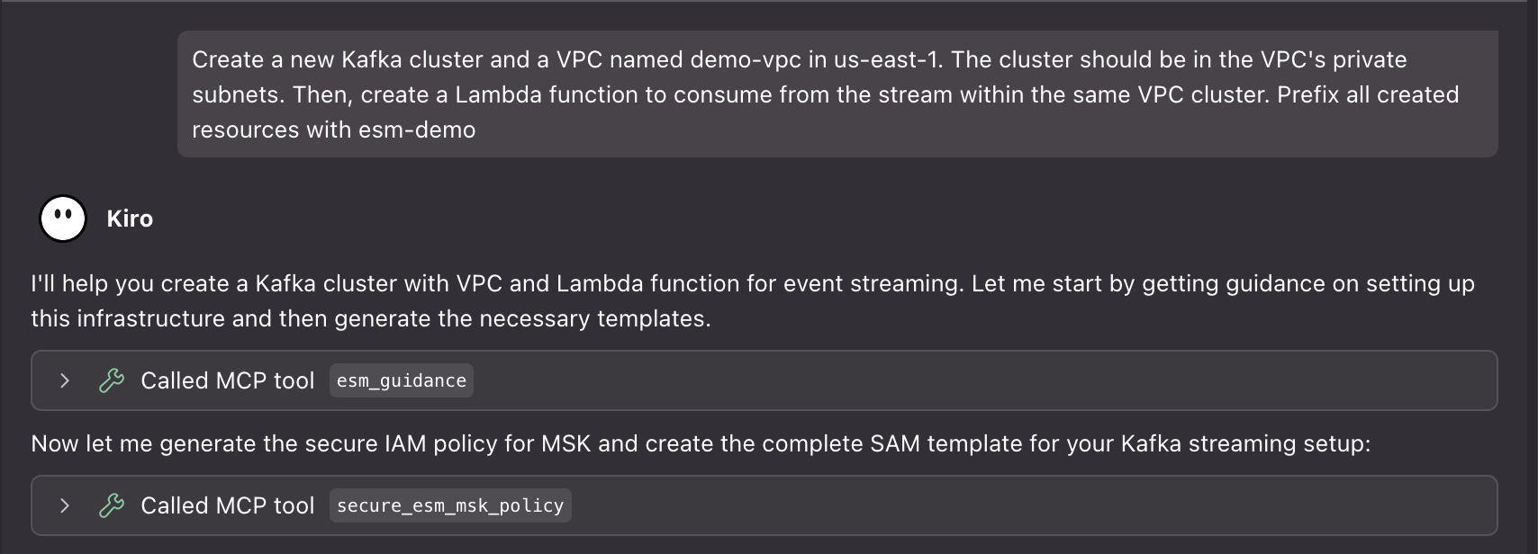
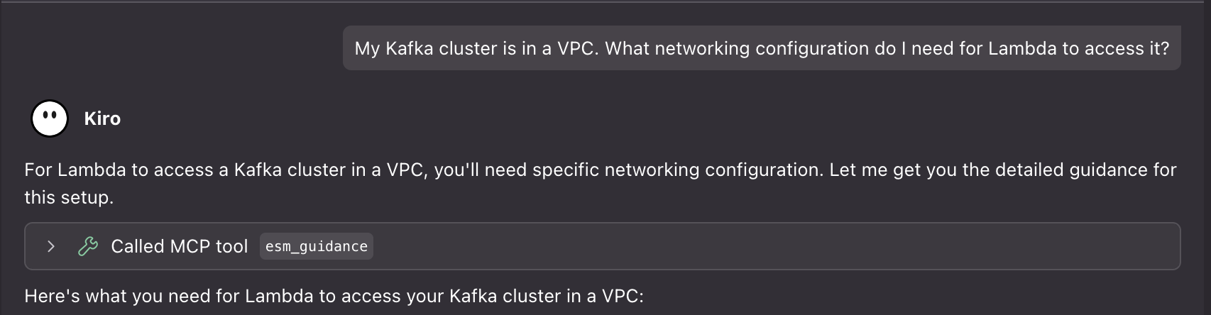
Data bucketing

To turn our protein vectors into a searchable database, we use LanceDB to build an index suitable for quickly finding ANNs to a query. However, indexing can take a long time and is difficult to distribute across nodes. To speed up indexing, we first divide our data into roughly evenly sized buckets. We then assign each of our embedding HDF5 files to buckets of size roughly equal to 200 million total vectors using a best-fit bin packing algorithm. The exact size packing method used to bucket data depends on the number and dimension of the vectors, as well as their format. Each bucket is ingested into a separate table that will separately reside in a single LanceDB database object store on Amazon S3.

S3 bucket structure showing LanceDB database organization with vector buckets

By bucketing our data, we can produce several smaller databases that can be indexed on separate nodes in a much shorter amount of time. We can also add more data to our database incrementally as a new bucket, instead of reindexing all the existing data.

Ingesting and indexing bucketed data

After the vectorized data has been assigned to a bucket, it’s time to turn it into a LanceDB table and index it to enable fast ANN querying. The details on how to convert your specific data into a LanceDB table can be found in the LanceDB documentation. For each of our buckets of approximately 200 million vectors, we create a LanceDB table with an IVF-PQ index on the cosine distance. For indexing, we use several partitions equal to the square root of the number of inserted rows, and several sub vectors equal to the number of dimensions of our vectors divided by 16.

To make things smoother to query, we name each table after the bucket from which it was created and upload them to a single S3 directory such that their file structure indicates a single LanceDB database with multiple tables.

The following code snippet provides an example of how you might ingest vectors from an HDF5 file containing id and embedding columns into a LanceDB database and index for fast ANN searches based on cosine distance. The only requirements for running this snippet are python >= 3.9, as well as the lancedb, pyarrow, and h5py packages. It should be noted that this snippet was tested and developed using lancedb version 0.21.1 using the asynchronous LanceDB API.

from typing import List, Iterable
from itertools import islice
from math import sqrt
import pyarrow as pa
import datetime
import asyncio
import lancedb
import h5py

def batched(iterable: Iterable, n: int) -> Iterable[List]:
    """Yield batches of n items from iterable."""
    while batch := list(islice(iterable, n)):
        yield batch

async def vectors_to_db(
    vectors: str,
    db: str,
    table_name: str,
    vector_dim: int,
    ingestion_batch_size: int,
) -> int:
    """Ingest and index vectors from an HDF5 file into a LanceDB table.
    Args:
        vectors (str): An HDF5 file containing protein IDs and their
            960-dimension vector representations.
        db (str): Path to the LanceDB database.
        table_name (str): Name of the table to create.
        vector_dim (int): Dimension of the vectors.
    """
    # create db and table
    custom_schema = pa.schema(
        [
            pa.field("embedding", pa.list_(pa.float32(), vector_dim)),
            pa.field("id", pa.string()),
        ]
    )

    # count the total number of rows as they are added to the table
    total_rows = 0

    # open a connection to the new database and create a table
    with await lancedb.connect_async(db) as db_connection:
        with await db_connection.create_table(
            table_name, schema=custom_schema
        ) as table_connection:
            # open vectors file
            with h5py.File(vectors, "r") as vectors_handle:
                # create a generator over the rows
                rows = (
                    {"embedding": e, "id": i}
                    for e, i in zip(
                        vectors_handle["embedding"],
                        vectors_handle["id"],
                    )
                )

                # insert rows in batches to avoid memory issues
                for batch in batched(rows, ingestion_batch_size):
                    total_rows += len(batch)
                    await table_connection.add(batch)

            # optimize the table and remove old data
            await table_connection.optimize(
                cleanup_older_than=datetime.timedelta(days=0)
            )

            # configure the index for the table
            index_config = lancedb.index.IvfPq(
                distance_type="cosine",
                num_partitions=int(sqrt(total_rows)),
                num_sub_vectors=int(
                    vector_dim / 16
                ),
            )

            # index the table
            await table_connection.create_index(
                "embedding", config=index_config
            )

# ingest and index your data
asyncio.run(
    vectors_to_db(
        vectors="./my_vectors.h5",
        db="./test_db",
        table_name="bucket1",
        vector_dim=960,
        ingestion_batch_size=50000
    )
)

The task of vectorizing, ingesting, indexing each bucket could be parallelized over multiple AWS Batch jobs or run on a single Amazon Elastic Compute Cloud (Amazon EC2) instance.

Querying the database

After the data has been bucketed and ingested into a LanceDB database on Amazon S3, we need a way to query it. Because LanceDB can be queried directly from Amazon S3 using the LanceDB Python API, we can use Lambda functions to take a user-provided query vector and search for ANNs, then return the data to the user. However, because our data has been bucketed across several tables in the database, we need to search for nearest neighbors in each bucket and aggregate the results before passing them back to the user.

We implement the query workflow as an AWS Step Functions state machine that manages a query process for each bucket as Lambda processes, as well as a single Lambda process at the end that aggregates the data and writes the resulting ANNs to a .csv file on Amazon S3. However, this could also be implemented as a series of AWS Batch processes or even run locally. The following snippet shows how a process assigned to one bucket could run an ANN query against one of the database’s buckets, requiring only pandas and lancedb to run on python >= 3.9. As detailed before in the ingestion section, we use the asynchronous LanceDB API and lancedb package version 0.21.1.

from typing import List, Iterable
import asyncio
import lancedb
import pandas
import random

async def run_query_async(
    lancedb_s3_uri: str,
    table_name: str,
    q_vec: List[float],
    k: int,
    vec_col: str,
    n_probes: int,
    refine_factor: int,
) -> pandas.DataFrame:
    """Run a query on a LanceDB table.
    Args:
        lancedb_s3_uri (str): S3 URI of the LanceDB database.
        table_name (str): Name of the table to query.
        q_vec (List[float]): Query vector.
        k (int): Number of nearest neighbors to return.
        vec_col (str): Column name of the vector column.
        n_probes (int): Number of probes to use for the query.
        refine_factor (int): Refine factor for the query.
    Returns:
        pandas.DataFrame: DataFrame containing the approximate nearest
        neighbors to the query vector.
    """
    # open a connection to the database and table
    with await lancedb.connect_async(
        lancedb_s3_uri, storage_options={"timeout": "120s"}
    ) as db_connection:
        with await db_connection.open_table(table_name) as table_connection:
            # query the approximate nearest neighbors to the query vector
            df = (
                await table_connection.query()
                .nearest_to(q_vec)
                .column(vec_col)
                .nprobes(n_probes)
                .refine_factor(refine_factor)
                .limit(k)
                .distance_type("cosine")
                .to_pandas()
            )

    return df

# query the example bucket we produced in the last section
bucket1_df = asyncio.run(
    snippets.run_query_async(
        lancedb_s3_uri="s3://mg-analysis/owen/20250415_lancedb_snippet_testing/test_db/",
        table_name="bucket1",
        q_vec=[random.random() for _ in range(960)],
        k=3,
        vec_col="embedding",
        n_probes=1,
        refine_factor=1,
    )
)

The preceding query will return a panda DataFrame of the following structure:

embedding id _distance
[-5.124435, 4.242000, …] id_1 0.000000
[-5.783999, 4.340500, …] id_2 0.001000
[-6.932943, 3.394850, …] id_3 0.04020

Where the embedding column contains the vector representations of the nearest neighbors, the id column their IDs, and the _distance column their cosine distances to the queried vector.

After each bucket has been independently queried across nodes and each has returned a nearest neighbors DataFrame, the results must be merged and subset to return the user. The following snippet shows how you might do this.

def aggregate_nearest_neighbors(
    dfs: List[pandas.DataFrame], k: int
):
    """Aggregate the nearest neighbors for each query vector.
    Args:
        dfs (List[pandas.DataFrame]): A list of DataFrames containing the
            nearest neighbors queried from each bucket.
        k (int): The number of nearest neighbors to aggregate.
    Returns:
        pd.DataFrame: A DataFrame with the aggregated nearest neighbors.
    """
    # concatenate the DataFrames and get the top k nearest neighbors
    return (
        pandas.concat(dfs, ignore_index=True)
        .sort_values(by=["_distance"], ascending=True)
        .reset_index(drop=True)
        .head(k)
    )

# add the dataframes from querying each bucket to a list
dfs = [bucket1_df, bucket2_df, bucket3_df, bucket4_df, bucket_5]

# aggregate the nearest neighbors across all buckets
nearest_neighbors_all_buckets_df = aggregate_nearest_neighbors(dfs, 5)

Optimizing for large batches of queries

Though querying a LanceDB database directly from its S3 object store on Lambda works well for querying the ANNs of one or a few query vectors, some use cases might require querying thousands or even millions of vectors.

One solution we’ve found that scales well to large batches of queries is to modify the preceding query implementation such that it first downloads one of the database buckets to local storage, then queries it locally using the LanceDB API. Because database buckets can have a large storage footprint, this implementation is better suited for AWS Batch jobs than Lambda, and we recommend using optimized instance storage (for example, i4i instances) rather than EBS volumes. After all query Batch jobs finish, a final job can aggregate their results before returning to the user. Orchestration of parallel query jobs and the aggregation job can be done with Nextflow. Though this implementation will have significantly more overhead and latency from downloading the buckets to disk, it can handle larger batches of queries more efficiently and still requires no continuously running server-based database.

Benchmarking results

Indexing strategies and database split sizes depend on your personal need for performance. Consider the following general optimization guidance when customizing to your use case.

An example database created by Metagenomi consisted of 3.5 billion vector embeddings produced by AMPLIFY, of dimension 960. Ingesting and indexing these 3.5B vector embeddings in split sizes of 200M vectors on i4i.8xlarge instances took 108 total compute hours. Because this solution is serverless and can be queried directly from its S3 object store, the only fixed cost of this database is its storage footprint on Amazon S3 (for an indexed database of 3.5B vectors, this is approximately 12.9 TB). Lambda queries can be an exceptionally low-cost querying solution, with many queries costing fractions of a cent.

In general, larger database splits will be more cost effective to query but will result in longer runtimes and longer indexing times. We recommend scaling up database split sizes to the maximum size that results in an acceptable query return time for a single split while also considering limits of parallelization such as maximum concurrent Lambda functions running. Metagenomi identified database splits of 200M vectors each to yield an optimal trade-off in cost and runtime for both small and large queries. We recommend ingesting and indexing on storage-optimized instances, such as those in the i4i family, for optimal performance and cost savings. If querying is to be done on an instance using a disk-based database (as opposed to Lambda and Amazon S3), we also recommend using storage-optimized instances for queries. We found the Lambda implementation could quickly handle single queries requesting up to 50,000 ANNs, or multi queries of up to 100 sequences with fewer than 5 ANNs. Runtime increases linearly with the number of ANNs requested, as shown in the following graph.

Line graph showing query runtime increasing with number of nearest neighbors

Conclusion

In this post, we showed how Metagenomi was able to store and query billions of protein embeddings at low cost using LanceDB implemented with Amazon S3 and AWS Lambda. This work expands on Metagenomi’s patient-driven mission to create curative genetic medicines by accelerating our discovery and engineering platform. Having quick access to the ANN embedding space of a query protein in seconds has enabled the integration of rapid search methods in our extensive analysis pipelines, accelerated the discovery of several diverse and novel enzyme families, and enabled protein engineering efforts by providing scientists with methods to generate and search embeddings on the fly. As Metagenomi continues to rapidly scale protein and DNA databases, horizontal scaling enabled by database splits that can be indexed and searched in parallel facilitates an embedding database solution that scales to future needs.

The solution outlined in this post focuses on vectors produced by a protein large language model (LLM) but can be applied to other vectorized datasets. To learn more about LanceDB integrated with Amazon S3, refer to the LanceDB documentation.

References

  1. Fournier, Quentin, et al. “Protein language models: is scaling necessary?.” bioRxiv (2024): 2024-09.

About the authors

Enhance the local testing experience for serverless applications with LocalStack

Post Syndicated from Patrick Galvin original https://aws.amazon.com/blogs/compute/enhance-the-local-testing-experience-for-serverless-applications-with-localstack/

Serverless applications often comprise multiple AWS services, such as AWS Lambda, Amazon Simple Queue Service (Amazon SQS), Amazon EventBridge, and Amazon DynamoDB. Although serverless architectures make it easy to build applications that are generally simple to operate and scale, testing them requires extra steps for developers. Recently, AWS brought you the capability to help developers remotely debug Lambda functions to accelerate the development process. Today, we’re excited to announce new capabilities that further simplify the local testing experience for Lambda functions and serverless applications through integration with LocalStack, an AWS Partner, in the AWS Toolkit for Visual Studio Code.

In this post, we will show you how you can enhance your local testing experience for serverless applications with LocalStack using AWS Toolkit.

Challenges with local serverless development

When building serverless applications with infrastructure as code (IaC) tools like the AWS Serverless Application Model (AWS SAM), developers often face challenges during local integration testing of applications that depend on interactions across multiple AWS services. These friction points slow down the critical code-test-debug cycle. Developers might encounter the following common roadblocks:

  • Cloud-based validation slows iteration – Developers previously needed to deploy AWS SAM templates to the cloud to test changes, introducing delays in feedback loops. AWS research shows that developers spend considerable time on deployment and testing, rather than writing code.
  • Tool context switching adds friction – Developers routinely shift between integrated development environments (IDEs), command line interfaces (CLIs), and resource emulators like LocalStack, leading to fragmented workflows.
  • Manual setup increases configuration complexity – Port mapping and code edits for local service integration tests can introduce inconsistencies between local and cloud environments.
  • Service integration debugging is limited – Troubleshooting Lambda functions in the context of AWS service integrations, such as DynamoDB, Amazon Simple Storage Service (Amazon S3), or Amazon SQS, requires manual configuration, extending the duration of troubleshooting efforts.

These challenges directly impact developer productivity and make local testing of integrated serverless applications complex.

Solution overview

Starting today, AWS helps simplify local serverless development by integrating LocalStack directly into the AWS Toolkit for VS Code. This integration helps developers test and debug serverless applications—defined using IaC tools like AWS SAM—entirely within their IDE. The enhanced local testing experience delivers four major improvements:

  • Integrated LocalStack experience – Connect to LocalStack directly within VS Code and manage local resources alongside cloud resources through a unified interface.
  • Emulated service interactions – Test Lambda functions with their interactions with other AWS services like Amazon SQS, DynamoDB, and EventBridge locally.
  • Simplified debugging – Start debugging sessions with LocalStack emulated environment, with a single click – no manual port configurations or code changes required, streamlining the debugging workflow.
  • Streamlined workflow – Deploy, test, and debug serverless applications without leaving the IDE, avoiding context switching between tools.

To set up LocalStack in VS Code (either the free version supporting over 30 core services like Lambda, Amazon S3, DynamoDB, Amazon SQS, and Amazon API Gateway, or the Ultimate version with over 110 services and advanced debugging features) you need essential development tools, including Docker, the AWS Command Line Interface (AWS CLI), AWS SAM CLI, and your preferred IDE such as VS Code. This combination enables full local integration testing of AWS services, including Lambda functions, messaging queues, databases, event-driven architectures, and serverless workflows, so you can develop and test your entire AWS application stack locally before deploying to the cloud.

Automated setup process

LocalStack is a cloud service emulator that you can use to run AWS applications locally for testing and development. To enhance your local testing capabilities, you can install the LocalStack VSCode Extension directly from AWS Walkthrough in AWS Toolkit, which offers a streamlined setup process through an intelligent wizard. After installation, the extension automatically detects whether LocalStack is configured on your system and prompts you to run the setup wizard through a notification. The entire process is quick and requires no manual configuration.

LocalStack extension has an integrated authentication wizard, that simplifies the process of connecting your development environment to LocalStack. During setup, the wizard opens a browser-based authentication flow and maintains an active connection until authentication completes. After it’s verified, it securely stores the authentication token in the ~/.localstack/auth.json file, enabling communication between your local environment and LocalStack services.

The wizard also checks if LocalStack AWS CLI profiles exist, and if not found, automatically creates them by updating the ~/.aws/config and ~/.aws/credentials files with LocalStack-specific endpoints and credentials. This seamless integration of AWS profiles enhances the development workflow by allowing developers to easily switch between different AWS environments, including the local LocalStack setup. By leveraging these profiles, developers can effortlessly point their AWS CLI or SDK to the appropriate endpoint, whether it’s a real AWS account or the LocalStack instance running on their machine. This configuration not only ensures a clear separation between local and cloud environments but also minimizes the risk of cross-environment interference. The automatic creation of these profiles streamlines the setup process, reducing manual configuration errors and saving valuable development time. Visual Studio Code (VS Code) provides real-time feedback throughout the setup. The status bar initially displays an error or warning indicator when LocalStack is not configured and then transitions to a normal or connected state once a successful connection is established. After setup completes, you’re ready to deploy, test, and debug serverless applications locally—without additional configuration. These settings persist across VS Code sessions, so the setup process is a one-time task.The following figure illustrates the process to start and verify LocalStack from VS Code.

To learn more, including installation steps, configuration examples, and troubleshooting guidance, visit the LocalStack Docs.

Test a serverless application

To demonstrate the enhanced local testing capabilities, let’s explore a practical serverless pattern: building and testing an event-driven order processing system that integrates Lambda with Amazon SQS, API Gateway, and Amazon Simple Notification Service (Amazon SNS). The application processes orders through an event-driven workflow: orders are submitted through API Gateway to an SQS queue and processed by a Lambda function, and the status is published to Amazon SNS to trigger customer email notifications.

Architechture digram depicting LocalStack emulation and user interaction with LocalStack emulated AWS Environment.

After you set up LocalStack in VS Code, you can test your entire serverless workflow without deploying to the cloud:

  • Deploy locally – Use the LocalStack AWS profile to deploy your AWS SAM application. The process mirrors cloud deployment but targets local endpoints. You can use the Application builder pane to initiate the deployment to LocalStack environment. The following figure illustrates the process of deploying a sample serverless application.

Picture depicting deploying a Serverless application on LocalStack and verifying the resources

  • Debug Lambda function deployed in LocalStack – Set breakpoints in your Lambda function and step through execution using VS Code’s integrated debugger. With the AWS Toolkit extension, you can invoke your Lambda with one click and inspect live interactions across services, all while running against a LocalStack container on your machine. This setup makes it possible to debug your AWS applications in a controlled, local environment that mimics the cloud infrastructure, without the need for deploying actual AWS services.

Picture depicting debugging a Lambda function using LocalStack and AWS VS Code Toolkit.

  • Validate end-to-end Flows – Test complete workflows from message ingestion through processing and notification, confirming all service integrations work correctly before cloud deployment.

For an in-depth technical demonstration of this LocalStack integration, refer to this youtube video.

Best practices for local Lambda function testing

In this section, we discuss various strategies and best practices for local Lambda function testing.

Optimizing your development workflow

Consider the following strategies to optimize your development workflow:

  • Start with a strong testing foundation – Use the AWS SAM CLI to perform unit tests that validate the core programmatic and business logic of your Lambda functions. Isolating function behavior early helps identify logic errors before introducing external dependencies.
  • Establish environment parity early in the development process – Many production issues stem from discrepancies between local and cloud environments. Use consistent service versions, configurations, and data structures across environments to confirm that what works locally behaves the same in production.
  • Adopt IaC from day one – Whether you choose AWS SAM, AWS CloudFormation, or another IaC framework, defining your application infrastructure as code reduces configuration drift and makes your deployments reproducible across teams and environments.
  • Apply a progressive testing strategy – Follow a structured testing pyramid that starts with fast, isolated unit tests and builds up to broader integration and system-level validation. This layered approach helps you catch issues earlier—when they’re easier and less expensive to fix—while still providing full application coverage.

A strategic approach to testing

Testing should be an integrated part of your serverless development workflow—not an afterthought. Successful teams implement layered testing strategies that use both local and cloud environments to strike a balance between speed and accuracy:

  1. Begin with unit tests that focus on isolated function logic. Use tools like the AWS SAM CLI, AWS Toolkit for VS Code and LocalStack extensions to run and debug functions locally.
  2. After validation, proceed to local integration testing using LocalStack to confirm how your Lambda functions interact with services such as Amazon SQS, DynamoDB, and Amazon SNS. These tests typically complete within minutes and catch most service integration issues before they reach production.
  3. After local testing, validate your application in the actual AWS environment. Cloud testing helps surface issues not present in local emulation, such as AWS Identity and Access Management (IAM) permission mismatches, Amazon Virtual Private Cloud (Amazon VPC) networking challenges, or service-specific nuances such as Lambda concurrency. For troubleshooting issues in the cloud environment, you can also remotely debug your Lambda functions using AWS Toolkit for VS Code.
  4. Lastly, conduct performance testing in AWS to assess how your application handles real-world traffic. These longer-running tests help validate scaling behavior and system resilience under load.

The result is higher-quality applications delivered faster, with fewer production surprises and more confident deployments.

Security considerations

When using LocalStack for local development, follow these security best practices:

  • Isolate the local environment – Use Docker networking to restrict LocalStack access and bind services to localhost to prevent external connections.
  • Use placeholder credentials – Use test credentials (for example, test/test) instead of real AWS credentials.
  • Protect your data – Use synthetic or anonymized datasets instead of production data and regularly purge local data stores to reduce risk.

When to use local versus cloud testing

Although local testing offers significant advantages, it’s important to understand when to use it versus testing in the cloud. The following table lists the potential use cases for each strategy.

Testing Scenario Local Testing Cloud Testing Reason
Function logic validation ✓ Fast feedback for core business logic
Service integration testing ✓ Quick validation of AWS service interactions
Rapid iteration during development ✓ Immediate feedback without deployment overhead
Cost-sensitive development environments ✓ Minimizes cloud resource costs during development
Offline development scenarios ✓ No internet connectivity required
Performance and scalability testing ✓ Requires actual AWS infrastructure for accurate results
IAM permission validation ✓ LocalStack doesn’t fully replicate IAM behavior
VPC networking scenarios ✓ Network configurations can’t be accurately emulated
Production-like load testing ✓ Real performance metrics only available in AWS
Final validation before deployment ✓ Supports compatibility with actual AWS environment

Conclusion

In this post, we discussed how to streamline local testing for AWS Serverless applications using LocalStack and the AWS Toolkit for VS Code. By running and debugging serverless applications directly in your IDE, you can reduce context switching, test complex integrations locally, and catch issues earlier—without deploying to the cloud.

We also showed how to apply progressive testing strategies that combine local emulation with cloud validation, optimize development costs, and build event-driven workflows with confidence.These enhancements lead to faster test cycles, lower development costs, and higher-quality deployments—all while staying fully in control of your development environment.

Have questions or feedback about this post? Connect with us on the AWS Compute Blog or join the AWS Developer community.

AWS named as a Leader in 2025 Gartner Magic Quadrant for Cloud-Native Application Platforms and Container Management

Post Syndicated from Channy Yun (윤석찬) original https://aws.amazon.com/blogs/aws/aws-named-as-a-leader-in-2025-gartner-magic-quadrant-for-cloud-native-application-platforms-and-container-management/

A month ago, I shared that Amazon Web Services (AWS) is recognized as a Leader in 2025 Gartner Magic Quadrant for Strategic Cloud Platform Services (SCPS), with Gartner naming AWS a Leader for the fifteenth consecutive year.

In 2024, AWS was named as a Leader in the Gartner Magic Quadrant for AI Code Assistants, Cloud-Native Application Platforms, Cloud Database Management Systems, Container Management, Data Integration Tools, Desktop as a Service (DaaS), and Data Science and Machine Learning Platforms as well as the SCPS. In 2025, we were also recognized as a Leader in the Gartner Magic Quadrant for Contact Center as a Service (CCaaS), Desktop as a Service and Data Science and Machine Learning (DSML) platforms. We strongly believe this means AWS provides the broadest and deepest range of services to customers.

Today, I’m happy to share recent Magic Quadrant reports that named AWS as a Leader in more cloud technology markets: Cloud-Native Application Platforms (aka Cloud Application Platforms) and Container Management.

2025 Gartner Magic Quadrant for Cloud-Native Application Platforms
AWS has been named a Leader in the Gartner Magic Quadrant for Cloud-Native Application Platforms for 2 consecutive years. AWS was positioned highest on “Ability to Execute”. Gartner defines cloud-native application platforms as those that provide managed application runtime environments for applications and integrated capabilities to manage the lifecycle of an application or application component in the cloud environment.

The following image is the graphical representation of the 2025 Magic Quadrant for Cloud-Native Application Platforms.

Our comprehensive cloud-native application portfolio—AWS Lambda, AWS App Runner, AWS Amplify, and AWS Elastic Beanstalk—offers flexible options for building modern applications with strong AI capabilities, demonstrated through continued innovation and deep integration across our broader AWS service portfolio.

You can simplify the service selection through comprehensive documentation, reference architectures, and prescriptive guidance available in the AWS Solutions Library, along with AI-powered, contextual recommendations from Amazon Q based on your specific requirements. While AWS Lambda is optimized for AWS to provide the best possible serverless experience, it follows industry standards for serverless computing and supports common programming languages and frameworks. You can find all necessary capabilities within AWS, including advanced features for AI/ML, edge computing, and enterprise integration.

You can build, deploy, and scale generative AI agents and applications by integrating these compute offerings with Amazon Bedrock for serverless inferences and Amazon SageMaker for artificial intelligence and machine learning (AI/ML) training and management.

Access the complete 2025 Gartner Magic Quadrant for Cloud-Native Application Platforms to learn more.

2025 Gartner Magic Quadrant for Container Management
In the 2025 Gartner Magic Quadrant for Container Management, AWS has been named as a Leader for three years and was positioned furthest for “Completeness of Vision”. Gartner defines container management as offerings that support the deployment and operation of containerized workloads. This process involves orchestrating and overseeing the entire lifecycle of containers, covering deployment, scaling, and operations, to ensure their efficient and consistent performance across different environments.

The following image is the graphical representation of the 2025 Magic Quadrant for Container Management.

AWS container services offer fully managed container orchestration with AWS native solutions and open-source technologies to focus on providing a wide range of deployment options, from Kubernetes to our native orchestrator.

You can use Amazon Elastic Container Service (Amazon ECS) and Amazon Elastic Kubernetes Service (Amazon EKS). Both can be used with AWS Fargate for serverless container deployment. Additionally, EKS Auto Mode simplifies Kubernetes management by automatically provisioning infrastructure, selecting optimal compute instances, and dynamically scaling resources for containerized applications.

You can connect on-premises and edge infrastructure back to AWS container services with EKS Hybrid Nodes and ECS Anywhere, or use EKS Anywhere for a fully disconnected Kubernetes experience supported by AWS. With flexible compute and deployment options, you can reduce operational overhead and focus on innovation and drive business value faster.

Access the complete 2025 Gartner Magic Quadrant for Container Management to learn more.

— Channy

Gartner does not endorse any vendor, product or service depicted in its research publications and does not advise technology users to select only those vendors with the highest ratings or other designation. Gartner research publications consist of the opinions of Gartner’s research organization and should not be construed as statements of fact. Gartner disclaims all warranties, expressed or implied, with respect to this research, including any warranties of merchantability or fitness for a particular purpose.

GARTNER is a registered trademark and service mark of Gartner and Magic Quadrant is a registered trademark of Gartner, Inc. and/or its affiliates in the U.S. and internationally and are used herein with permission. All rights reserved.

AWS Weekly Roundup: Strands Agents 1M+ downloads, Cloud Club Captain, AI Agent Hackathon, and more (September 15, 2025)

Post Syndicated from Channy Yun (윤석찬) original https://aws.amazon.com/blogs/aws/aws-weekly-roundup-strands-agents-1m-downloads-cloud-club-captain-ai-agent-hackathon-and-more-september-15-2025/

Last week, Strands Agents, AWS open source for agentic AI SDK just hit 1 million downloads and earned 3,000+ GitHub Stars less than 4 months since launching as a preview in May 2025. With Strands Agents, you can build production-ready, multi-agent AI systems in a few lines of code.

We’ve continuously improved features including support for multi-agent patterns, A2A protocol, and Amazon Bedrock AgentCore. You can use a collection of sample implementations to help you get started with building intelligent agents using Strands Agents. We always welcome your contribution and feedback to our project including bug reports, new features, corrections, or additional documentation.

Here is the latest research article of Amazon Science about the future of agentic AI and questions that scientists are asking about agent-to-agent communications, contextual understanding, common sense reasoning, and more. You can understand the technical topic of agentic AI with with relatable examples, including one about our personal behaviors about leaving doors open or closed, locked or unlocked.

Last week’s launches
Here are some launches that got my attention:

  • Amazon EC2 M4 and M4 Pro Mac instances – New M4 Mac instances offer up to 20% better application build performance compared to M2 Mac instances, while M4 Pro Mac instances deliver up to 15% better application build performance compared to M2 Pro Mac instances. These instances are ideal for building and testing applications for Apple platforms such as iOS, macOS, iPadOS, tvOS, watchOS, visionOS, and Safari.
  • LocalStack integration in Visual Studio Code (VS Code) – You can use LocalStack to locally emulate and test your serverless applications using the familiar VS Code interface without switching between tools or managing complex setup, thus simplifying your local serverless development process.
  • AWS Cloud Development Kit (AWS CDK) Refactor (Preview) –You can rename constructs, move resources between stacks, and reorganize CDK applications while preserving the state of deployed resources. By using AWS CloudFormation’s refactor capabilities with automated mapping computation, CDK Refactor eliminates the risk of unintended resource replacement during code restructuring.
  • AWS CloudTrail MCP Server – New AWS CloudTrail MCP server allows AI assistants to analyze API calls, track user activities, and perform advanced security analysis across your AWS environment through natural language interactions. You can explore more AWS MCP servers for working with AWS service resources.
  • Amazon CloudFront support for IPv6 origins – Your applications can send IPv6 traffic all the way to their origins, allowing them to meet their architectural and regulatory requirements for IPv6 adoption. End-to-end IPv6 support improves network performance for end users connecting over IPv6 networks, and also removes concerns for IPv4 address exhaustion for origin infrastructure.

For a full list of AWS announcements, be sure to keep an eye on the What’s New with AWS? page.

Other AWS news
Here are some additional news items that you might find interesting:

  • A city in the palm of your hand – Check out this interactive feature that explains how our AWS Trainium chip designers think like city planners, optimizing every nanometer to move data at near light speed.
  • Measuring the effectiveness of software development tools and practices – Read how Amazon developers that identified specific challenges before adopting AI tools cut costs by 15.9% year-over-year using our cost-to-serve-software framework (CTS-SW). They deployed more frequently and reduced manual interventions by 30.4% by focusing on the right problems first.
  • Become an AWS Cloud Club Captain – Join a growing network of student cloud enthusiasts by becoming an AWS Cloud Club Captain! As a Captain, you’ll get to organize events and building cloud communities while developing leadership skills. Application window is open September 1-28, 2025.

Upcoming AWS events
Check your calendars and sign up for these upcoming AWS events as well as AWS re:Invent and AWS Summits:

  • AWS AI Agent Global Hackathon – This is your chance to dive deep into our powerful generative AI stack and create something truly awesome. From September 8 to October 20, you have the opportunity to create AI agents using AWS suite of AI services, competing for over $45,000 in prizes and exclusive go-to-market opportunities.
  • AWS Gen AI Lofts – You can learn AWS AI products and services with exclusive sessions and meet industry-leading experts, and have valuable networking opportunities with investors and peers. Register in your nearest city: Mexico City (September 30–October 2), Paris (October 7–21), London (Oct 13–21), and Tel Aviv (November 11–19).
  • AWS Community Days – Join community-led conferences that feature technical discussions, workshops, and hands-on labs led by expert AWS users and industry leaders from around the world: Aotearoa and Poland (September 18), South Africa (September 20), Bolivia (September 20), Portugal (September 27), Germany (October 7), and Hungary (October 16).

You can browse all upcoming AWS events and AWS startup events.

That’s all for this week. Check back next Monday for another Weekly Roundup!

— Channy