How the “Frontier” Became the Slogan of Uncontrolled AI

Post Syndicated from B. Schneier original https://www.schneier.com/blog/archives/2024/02/how-the-frontier-became-the-slogan-of-uncontrolled-ai.html

Artificial intelligence (AI) has been billed as the next frontier of humanity: the newly available expanse whose exploration will drive the next era of growth, wealth, and human flourishing. It’s a scary metaphor. Throughout American history, the drive for expansion and the very concept of terrain up for grabs—land grabs, gold rushes, new frontiers—have provided a permission structure for imperialism and exploitation. This could easily hold true for AI.

This isn’t the first time the concept of a frontier has been used as a metaphor for AI, or technology in general. As early as 2018, the powerful foundation models powering cutting-edge applications like chatbots have been called “frontier AI.” In previous decades, the internet itself was considered an electronic frontier. Early cyberspace pioneer John Perry Barlow wrote “Unlike previous frontiers, this one has no end.” When he and others founded the internet’s most important civil liberties organization, they called it the Electronic Frontier Foundation.

America’s experience with frontiers is fraught, to say the least. Expansion into the Western frontier and beyond has been a driving force in our country’s history and identity—and has led to some of the darkest chapters of our past. The tireless drive to conquer the frontier has directly motivated some of this nation’s most extreme episodes of racism, imperialism, violence, and exploitation.

That history has something to teach us about the material consequences we can expect from the promotion of AI today. The race to build the next great AI app is not the same as the California gold rush. But the potential that outsize profits will warp our priorities, values, and morals is, unfortunately, analogous.

Already, AI is starting to look like a colonialist enterprise. AI tools are helping the world’s largest tech companies grow their power and wealth, are spurring nationalistic competition between empires racing to capture new markets, and threaten to supercharge government surveillance and systems of apartheid. It looks more than a bit like the competition among colonialist state and corporate powers in the seventeenth century, which together carved up the globe and its peoples. By considering America’s past experience with frontiers, we can understand what AI may hold for our future, and how to avoid the worst potential outcomes.

America’s “Frontier” Problem

For 130 years, historians have used frontier expansion to explain sweeping movements in American history. Yet only for the past thirty years have we generally acknowledged its disastrous consequences.

Frederick Jackson Turner famously introduced the frontier as a central concept for understanding American history in his vastly influential 1893 essay. As he concisely wrote, “American history has been in a large degree the history of the colonization of the Great West.”

Turner used the frontier to understand all the essential facts of American life: our culture, way of government, national spirit, our position among world powers, even the “struggle” of slavery. The endless opportunity for westward expansion was a beckoning call that shaped the American way of life. Per Turner’s essay, the frontier resulted in the individualistic self-sufficiency of the settler and gave every (white) man the opportunity to attain economic and political standing through hardscrabble pioneering across dangerous terrain.The New Western History movement, gaining steam through the 1980s and led by researchers like Patricia Nelson Limerick, laid plain the racial, gender, and class dynamics that were always inherent to the frontier narrative. This movement’s story is one where frontier expansion was a tool used by the white settler to perpetuate a power advantage.The frontier was not a siren calling out to unwary settlers; it was a justification, used by one group to subjugate another. It was always a convenient, seemingly polite excuse for the powerful to take what they wanted. Turner grappled with some of the negative consequences and contradictions of the frontier ethic and how it shaped American democracy. But many of those whom he influenced did not do this; they celebrated it as a feature, not a bug. Theodore Roosevelt wrote extensively and explicitly about how the frontier and his conception of white supremacy justified expansion to points west and, through the prosecution of the Spanish-American War, far across the Pacific. Woodrow Wilson, too, celebrated the imperial loot from that conflict in 1902. Capitalist systems are “addicted to geographical expansion” and even, when they run out of geography, seek to produce new kinds of spaces to expand into. This is what the geographer David Harvey calls the “spatial fix.”Claiming that AI will be a transformative expanse on par with the Louisiana Purchase or the Pacific frontiers is a bold assertion—but increasingly plausible after a year dominated by ever more impressive demonstrations of generative AI tools. It’s a claim bolstered by billions of dollars in corporate investment, by intense interest of regulators and legislators worldwide in steering how AI is developed and used, and by the variously utopian or apocalyptic prognostications from thought leaders of all sectors trying to understand how AI will shape their sphere—and the entire world.

AI as a Permission Structure

Like the western frontier in the nineteenth century, the maniacal drive to unlock progress via advancement in AI can become a justification for political and economic expansionism and an excuse for racial oppression.

In the modern day, OpenAI famously paid dozens of Kenyans little more than a dollar an hour to process data used in training their models underlying products such as ChatGPT. Paying low wages to data labelers surely can’t be equated to the chattel slavery of nineteenth-century America. But these workers did endure brutal conditions, including being set to constantly review content with “graphic scenes of violence, self-harm, murder, rape, necrophilia, child abuse, bestiality, and incest.” There is a global market for this kind of work, which has been essential to the most important recent advances in AI such as Reinforcement Learning with Human Feedback, heralded as the most important breakthrough of ChatGPT.

The gold rush mentality associated with expansion is taken by the new frontiersmen as permission to break the rules, and to build wealth at the expense of everyone else. In 1840s California, gold miners trespassed on public lands and yet were allowed to stake private claims to the minerals they found, and even to exploit the water rights on those lands. Again today, the game is to push the boundaries on what rule-breaking society will accept, and hope that the legal system can’t keep up.

Many internet companies have behaved in exactly the same way since the dot-com boom. The prospectors of internet wealth lobbied for, or simply took of their own volition, numerous government benefits in their scramble to capture those frontier markets. For years, the Federal Trade Commission has looked the other way or been lackadaisical in halting antitrust abuses by Amazon, Facebook, and Google. Companies like Uber and Airbnb exploited loopholes in, or ignored outright, local laws on taxis and hotels. And Big Tech platforms enjoyed a liability shield that protected them from punishment the contents people posted to their sites.

We can already see this kind of boundary pushing happening with AI.

Modern frontier AI models are trained using data, often copyrighted materials, with untested legal justification. Data is like water for AI, and, like the fight over water rights in the West, we are repeating a familiar process of public acquiescence to private use of resources. While some lawsuits are pending, so far AI companies have faced no significant penalties for the unauthorized use of this data.

Pioneers of self-driving vehicles tried to skip permitting processes and used fake demonstrations of their capabilities to avoid government regulation and entice consumers. Meanwhile, AI companies’ hope is that they won’t be held to blame if the AI tools they produce spew out harmful content that causes damage in the real world. They are trying to use the same liability shield that fostered Big Tech’s exploitation of the previous electronic frontiers—the web and social media—to protect their own actions.

Even where we have concrete rules governing deleterious behavior, some hope that using AI is itself enough to skirt them. Copyright infringement is illegal if a person does it, but would that same person be punished if they train a large language model to regurgitate copyrighted works? In the political sphere, the Federal Election Commission has precious few powers to police political advertising; some wonder if they simply won’t be considered relevant if people break those rules using AI.

AI and American Exceptionalism

Like The United States’ historical frontier, AI has a feel of American exceptionalism. Historically, we believed we were different from the Old World powers of Europe because we enjoyed the manifest destiny of unrestrained expansion between the oceans. Today, we have the most CPU power, the most data scientists, the most venture-capitalist investment, and the most AI companies. This exceptionalism has historically led many Americans to believe they don’t have to play by the same rules as everyone else.

Both historically and in the modern day, this idea has led to deleterious consequences such as militaristic nationalism (leading to justifying of foreign interventions in Iraq and elsewhere), masking of severe inequity within our borders, abdication of responsibility from global treaties on climate and law enforcement, and alienation from the international community. American exceptionalism has also wrought havoc on our country’s engagement with the internet, including lawless spying and surveillance by forces like the National Security Agency.

The same line of thinking could have disastrous consequences if applied to AI. It could perpetuate a nationalistic, Cold War–style narrative about America’s inexorable struggle with China, this time predicated on an AI arms race. Moral exceptionalism justifies why we should be allowed to use tools and weapons that are dangerous in the hands of a competitor, or enemy. It could enable the next stage of growth of the military-industrial complex, with claims of an urgent need to modernize missile systems and drones through using AI. And it could renew a rationalization for violating civil liberties in the US and human rights abroad, empowered by the idea that racial profiling is more objective if enforced by computers.The inaction of Congress on AI regulation threatens to land the US in a regime of de facto American exceptionalism for AI. While the EU is about to pass its comprehensive AI Act, lobbyists in the US have muddled legislative action. While the Biden administration has used its executive authority and federal purchasing power to exert some limited control over AI, the gap left by lack of legislation leaves AI in the US looking like the Wild West—a largely unregulated frontier.The lack of restraint by the US on potentially dangerous AI technologies has a global impact. First, its tech giants let loose their products upon the global public, with the harms that this brings with it. Second, it creates a negative incentive for other jurisdictions to more forcefully regulate AI. The EU’s regulation of high-risk AI use cases begins to look like unilateral disarmament if the US does not take action itself. Why would Europe tie the hands of its tech competitors if the US refuses to do the same?

AI and Unbridled Growth

The fundamental problem with frontiers is that they seem to promise cost-free growth. There was a constant pressure for American westward expansion because a bigger, more populous country accrues more power and wealth to the elites and because, for any individual, a better life was always one more wagon ride away into “empty” terrain. AI presents the same opportunities. No matter what field you’re in or what problem you’re facing, the attractive opportunity of AI as a free labor multiplier probably seems like the solution; or, at least, makes for a good sales pitch.

That would actually be okay, except that the growth isn’t free. America’s imperial expansion displaced, harmed, and subjugated native peoples in the Americas, Africa, and the Pacific, while enlisting poor whites to participate in the scheme against their class interests. Capitalism makes growth look like the solution to all problems, even when it’s clearly not. The problem is that so many costs are externalized. Why pay a living wage to human supervisors training AI models when an outsourced gig worker will do it at a fraction of the cost? Why power data centers with renewable energy when it’s cheaper to surge energy production with fossil fuels? And why fund social protections for wage earners displaced by automation if you don’t have to? The potential of consumer applications of AI, from personal digital assistants to self-driving cars, is irresistible; who wouldn’t want a machine to take on the most routinized and aggravating tasks in your daily life? But the externalized cost for consumers is accepting the inevitability of domination by an elite who will extract every possible profit from AI services.

Controlling Our Frontier Impulses

None of these harms are inevitable. Although the structural incentives of capitalism and its growth remain the same, we can make different choices about how to confront them.

We can strengthen basic democratic protections and market regulations to avoid the worst impacts of AI colonialism. We can require ethical employment for the humans toiling to label data and train AI models. And we can set the bar higher for mitigating bias in training and harm from outputs of AI models.

We don’t have to cede all the power and decision making about AI to private actors. We can create an AI public option to provide an alternative to corporate AI. We can provide universal access to ethically built and democratically governed foundational AI models that any individual—or company—could use and build upon.

More ambitiously, we can choose not to privatize the economic gains of AI. We can cap corporate profits, raise the minimum wage, or redistribute an automation dividend as a universal basic income to let everyone share in the benefits of the AI revolution. And, if these technologies save as much labor as companies say they do, maybe we can also all have some of that time back.

And we don’t have to treat the global AI gold rush as a zero-sum game. We can emphasize international cooperation instead of competition. We can align on shared values with international partners and create a global floor for responsible regulation of AI. And we can ensure that access to AI uplifts developing economies instead of further marginalizing them.

This essay was written with Nathan Sanders, and was originally published in Jacobin.

Extending Zabbix: the power of scripting

Post Syndicated from Giedrius Stasiulionis original https://blog.zabbix.com/extending-zabbix-the-power-of-scripting/27401/

Scripts can extend Zabbix in various different aspects. If you know your ways around a CLI, you will be able to extend your monitoring capabilities and streamline workflows related to most Zabbix components.

What I like about Zabbix is that it is very flexible and powerful tool right out of the box. It has many different ways to collect, evaluate and visualize data, all implemented natively and ready to use.

However, in more complex environments or custom use cases, you will inevitably face situations when something can’t be collected (or displayed) in a way that you want. Luckily enough, Zabbix is flexible even here! It provides you with ways to apply your knowledge and imagination so that even most custom monitoring scenarios would be covered. Even though Zabbix is an open-source tool, in this article I will talk about extending it without changing its code, but rather by applying something on top, with the help of scripting. I will guide you through some examples, which will hopefully pique your curiosity and maybe you will find them interesting enough to experiment and create something similar for yourself.

Although first idea which comes to ones mind when talking about scripts in Zabbix is most likely data collection, it is not the only place where scripts can help. So I will divide those examples / ideas into three sub categories:

  • Data collection
  • Zabbix internals
  • Visualization

Data collection

First things first. Data collection is a starting point for any kind of monitoring. There are multiple ways how to collect data in “custom” ways, but the easiest one is to use UserParameter capabilities. Basics of it are very nicely covered by official documentation or in other sources, e.g. in this video by Dmitry Lambert, so I will skip the “Hello World” part and provide some more advanced ideas which might be useful to consider. Also, the provided examples use common scripting themes/scenarios and you can find many similar solutions in the community, so maybe this will serve better as a reminder or a showcase for someone who has never created any custom items before.

Data collection: DB checks

There is a lot of good information on how to setup DB checks for Zabbix, so this is just a reminder, that one of the ways to do it is via custom scripts. I personally have done it for various different databases: MySQL, Oracle, PostgreSQL, OpenEdge Progress. Thing is ODBC is not always a great or permitted way to go, since some security restrictions might be in place and you can’t get direct access to DB from just anywhere you want. Or you want to transform your retrieved data in a ways that are complex and could hardly be covered by preprocessing. Then you have to rely on Zabbix agent running those queries either from localhost where DB resides or from some other place which is allowed to connect to your DB. Here is an example how you can do it for PostgreSQL

#!/bin/bash

my_dir="$(dirname ${0})"
conf_file="${my_dir}/sms_queue.conf"

[[ ! -f $conf_file ]] && echo -1 && exit 1

. ${conf_file}

export PGPASSWORD="${db_pass}"

query="SELECT COUNT(*) FROM sms WHERE sms.status IN ('retriable', 'validated');"

psql -h "${db_host}" -p "${db_port}" -U "${db_user}" -d "${db}" -c "${query}" -At 2>/dev/null

[[ $? -ne 0 ]] && echo -1 && exit 1

exit 0

Now what’s left is to feed the output of this script into Zabbix via UserParameter. Similar approach can be applied to Oracle (via sqlplus) or MySQL.

Data collection: log delay statistics

I once faced a situation when some graphs which are based on log data started having gaps. It meant something was wrong either with data collection (Zabbix agent) or with data not being there at the moment of collection (so nothing to collect). Quick check suggested it was the second one, but I needed to prove it somehow.

Since these log lines had timestamps of creation, it was a logical step to try to measure, how much do they differ from “current time” of reading. And this is how I came up with the following custom script to implement such idea.

First of all, we need to read the file, say once each minute. We are talking about log with several hundreds of thousands lines per minute, so this script should be made efficient. It should read the file in portions created between two script runs. I have explained such reading in details here so now we will not focus on it.

Next what this script does is it greps timestamps only from each line and counts immediately number of unique lines with the same timestamp (degree of seconds). That is where it becomes fast – it doesn’t need to analyze each and every line individually but it can analyze already grouped content!

Finally, delay is calculated based on the difference between “now” and collected timestamps, and those counters are exactly what is then passed to Zabbix.

#!/bin/bash

my_log="${1}"

my_project="${my_log##*\/}"
my_project="${my_project%%.log}"

me="$(basename ${0})"
my_dir="/tmp/log_delays/${my_project}"

[[ ! -d ${my_dir} ]] && mkdir -p ${my_dir}

# only one instance of this script at single point of time
# this makes sure you don't damage temp files

me_running="${my_dir}/${me}.running"

# allow only one process
# but make it more sophisticated:
# script is being run each minute
# if .running file is here for more than 10 minutes, something is wrong
# delete .running and try to run once again

[[ -f $me_running && $(($(date +%s)-$(stat -c %Y $me_running))) -lt 600 ]] && exit 1

touch $me_running

[[ "${my_log}" == "" || ! -f "${my_log}" ]] && exit 1

log_read="${my_dir}/${me}.read"

# get current file size in bytes

current_size=$(wc -c < "${my_log}")

# remember how many bytes you have now for next read
# when run for first time, you don't know the previous

[[ ! -f "${log_read}" ]] && echo "${current_size}" > "${log_read}"

bytes_read=$(cat "${log_read}")
echo "${current_size}" > "${log_read}"

# if rotated, let's read from the beginning

if [[ ${bytes_read} -gt ${current_size} ]]; then
  bytes_read=0
fi


# get the portion

now=$(date +%s)

delay_1_min=0
delay_5_min=0
delay_10_min=0
delay_30_min=0
delay_45_min=0
delay_60_min=0
delay_rest=0

while read line; do

  [[ ${line} == "" ]] && continue

  line=(${line})

  ts=$(date -d "${line[1]}+00:00" +%s)

  delay=$((now-ts))

  if [[ ${delay} -lt 60 ]]; then
    delay_1_min=$((${delay_1_min}+${line[0]}))
  elif [[ ${delay} -lt 300 ]]; then
    delay_5_min=$((${delay_5_min}+${line[0]}))
  elif [[ ${delay} -lt 600 ]]; then
    delay_10_min=$((${delay_10_min}+${line[0]}))
  elif [[ ${delay} -lt 1800 ]]; then
    delay_30_min=$((${delay_30_min}+${line[0]}))
  elif [[ ${delay} -lt 2700 ]]; then
    delay_45_min=$((${delay_45_min}+${line[0]}))
  elif [[ ${delay} -lt 3600 ]]; then
    delay_60_min=$((${delay_60_min}+${line[0]}))
  else
    delay_rest=$((${delay_rest}+${line[0]}))
  fi

done <<< "$(tail -c +$((bytes_read+1)) "${my_log}" | head -c $((current_size-bytes_read)) | grep -Po "(?<=timestamp\":\")(\d{4}-\d{2}-\d{2}T\d{2}:\d{2}:\d{2})(?=\.)" | sort | uniq -c | sort -k1nr)"

echo "delay_1_min=${delay_1_min}
delay_5_min=${delay_5_min}
delay_10_min=${delay_10_min}
delay_30_min=${delay_30_min}
delay_45_min=${delay_45_min}
delay_60_min=${delay_60_min}
delay_rest=${delay_rest}"


rm -f "${me_running}"

exit 0

Now on Zabbix side, there is an item running this script and 7 dependent items, representing the degree of delay. Since there are many logs for which this data is collected, it is all put into LLD based on contents of specific directory:

vfs.dir.get[/var/log/logs,".*log$",,,,,1000]

This LLD then provides two macros:

And item prototypes will look like:

Those dependent items have one simple preprocessing step which takes needed number out of the script output:

So the final result is the nice graph in dashboard, showing exactly when and what degree delays do appear:

So as you see, it is relatively easy to collect just about any data you wish, once you know how. As you can see from these examples, it might be something more complex but it can also be just a simple one-liner – in any case it should be obvious that possibilities are endless when talking about scripts in data collection. If something is executable from the CLI and has a valuable output, go ahead and collect it!

Zabbix internals

Another area where scripts can be really useful is adjusting how Zabbix behaves or controlling this behavior automatically. And in this case, we will employ Zabbix API, since it’s designed exactly for such or similar purposes.

Zabbix internals: automatically disabling problematic item

In our environment, we have many logs to be analyzed. And some of them sometimes go crazy – something that we intend to catch starts appearing there too often and requires attention – typically we would have to adjust the regexp, temporarily suppress some patterns and inform responsible teams about too extensive logging. If you don’t (or can’t) pay attention quick, it might kill Zabbix – history write cache starts filling up. So what we do is automatically detect such an item with most values received during some most recent short period of time and automatically disable it.

First of all there are two items – the one measuring history write cache and the other one extracting top item in the given table

[root@linux ~]# zabbix_agentd -t zabbix.db.max[history_log,30] 2>/dev/null
zabbix.db.max[history_log,30] [t|463 1997050]
[root@linux ~]#

First number here is values gathered during provided period, second one is item id. The script behind this item looks like this

[root@linux ~]# grep zabbix.db.max /etc/zabbix/zabbix_agentd.d/userparameter_mysql.conf
UserParameter=zabbix.db.max[*],HOME=/etc/zabbix mysql -BN -e "USE zabbix; SELECT count(*), itemid FROM $1 WHERE clock >= unix_timestamp(NOW() - INTERVAL $2 MINUTE) GROUP BY itemid ORDER BY count(*) DESC LIMIT 1;"
[root@linux ~]#

And now relying on the history write cache item values showing us drop, we construct a trigger:

And as a last step, such trigger invokes action, which is running the script that disables the item with given ID with the help of Zabbix API, method “item.update”

Now we are able to avoid unexpected behavior of our data sources affecting Zabbix performance, all done automatically – thanks to the scripts!

Zabbix internals: add host to group via frontend scripts

Zabbix maintenance mode is a great feature allowing us to reduce noise or avoid some false positive alerts once specific host is known to have issues. At some point we found it would be convenient to be able to add (or remove) specific host into (from) maintenance directly from “Problems” window. And that is possible and achieved via a frontend script, again with the help of Zabbix API, this time methods “host.get”, “hostgroup.get”, “hostgroup.massadd” and “hostgroup.massremove”

Data visualization

Zabbix has many different widgets that are able to cover various different ways of displaying your collected data. But in some cases, you might find yourself missing some small type of “something” which would allow your dashboards to shine even more – at least I constantly face it. Starting From version 6.4 Zabbix allows you to create your own widgets but it might be not such a straightforward procedure if you have little or no programming experience. However, you can employ two already existing widgets in order to customize your dashboard look in pretty easy way.

Data visualization: URL widget

First one example is done using the URL widget. You might feed just about any content there, so if you have any web development skills, you can easily create something which would look like custom widget. Here is an example. I need a clock but not the one already provided by Zabbix as a separate clock widget – I want to have a digital clock and I also want this clock to have a section, which would display the employee on duty now and in an upcoming shift. So with a little bit of HTML, CSS and JavaScript / AJAX, I have this

With styles properly chosen, such content can be smoothly integrated into dashboards, along with other widgets.

Data visualization: plain text widget with HTML formatting

Another useful widget which is often overlooked is the “Plain text” widget – in combination with the following parameters:

It becomes a very powerful tool to display nicely formatted data snapshots. Simple yet very good example here would be to display some content, which requires human readable structure – a table.

So again, integration with other dashboard widgets is so smooth – with just some custom HTML / CSS around your data you wrap it into something that looks like brand new “table” widget. Isn’t it awesome? And you are of course not limited to tables… Just use your imagination!

Conclusion

Although I personally prefer bash as the first option to solve things, there is no big difference regarding which scripting or programming languages to choose when extending Zabbix in these ways. Just try anything you feel most comfortable with.

I hope that examples shown here inspired you in some ways. Happy scripting!

The post Extending Zabbix: the power of scripting appeared first on Zabbix Blog.

След смъртта на Навални, руската опозиция се активира във въоръжена борба срещу Путин Легион за свободата на Русия действа и в България

Post Syndicated from Екип на Биволъ original https://bivol.bg/legion_freedom_russia.html

четвъртък 29 февруари 2024


Военизирана организация на руски граждани и етнически руснаци, живеещи в Украйна и в емиграция отправи свое послание към българската общественост. Структурата се нарича Легион за Свобода на Русия /Легион Свобода…

Да купуваме ли имот сега или да изчакаме?

Post Syndicated from VassilKendov original https://kendov.com/%D0%B4%D0%B0-%D0%BA%D1%83%D0%BF%D1%83%D0%B2%D0%B0%D0%BC%D0%B5-%D0%BB%D0%B8-%D0%B8%D0%BC%D0%BE%D1%82-%D1%81%D0%B5%D0%B3%D0%B0-%D0%B8%D0%BB%D0%B8-%D0%B4%D0%B0-%D0%B8%D0%B7%D1%87%D0%B0%D0%BA%D0%B0%D0%BC/

В кои случаи е обоснована покупката на недвижим имот в момента?

– При защита на спестяванията от инфлация
– Решаване на реален проблем с местообитанието
– При пране на средства с произход корупция или забранени дейности
– При доходи от собствен бизнес, поради очакване на свиване на кредитирането


Моля използвайте приложената форма за записване на час за среща
[contact-form-7]

The post Да купуваме ли имот сега или да изчакаме? appeared first on Kendov.com.

AMD EPYC Bergamo Has Massive Consolidation Benefits

Post Syndicated from Patrick Kennedy original https://www.servethehome.com/amd-epyc-bergamo-has-massive-consolidation-benefits-supermicro/

We show the massive consolidation with AMD EPYC Bergamo. An 8x GPU AI server can fit in the power and space saved with just 3 Bergamo servers

The post AMD EPYC Bergamo Has Massive Consolidation Benefits appeared first on ServeTheHome.

Top Architecture Blog Posts of 2023

Post Syndicated from Andrea Courtright original https://aws.amazon.com/blogs/architecture/top-architecture-blog-posts-of-2023/

2023 was a rollercoaster year in tech, and we at the AWS Architecture Blog feel so fortunate to have shared in the excitement. As we move into 2024 and all of the new technologies we could see, we want to take a moment to highlight the brightest stars from 2023.

As always, thanks to our readers and to the many talented and hardworking Solutions Architects and other contributors to our blog.

I give you our 2023 cream of the crop!

#10: Build a serverless retail solution for endless aisle on AWS

In this post, Sandeep and Shashank help retailers and their customers alike in this guided approach to finding inventory that doesn’t live on shelves.

Building endless aisle architecture for order processing

Figure 1. Building endless aisle architecture for order processing

Check it out!

#9: Optimizing data with automated intelligent document processing solutions

Who else dreads wading through large amounts of data in multiple formats? Just me? I didn’t think so. Using Amazon AI/ML and content-reading services, Deependra, Anirudha, Bhajandeep, and Senaka have created a solution that is scalable and cost-effective to help you extract the data you need and store it in a format that works for you.

AI-based intelligent document processing engine

Figure 2: AI-based intelligent document processing engine

Check it out!

#8: Disaster Recovery Solutions with AWS managed services, Part 3: Multi-Site Active/Passive

Disaster recovery posts are always popular, and this post by Brent and Dhruv is no exception. Their creative approach in part 3 of this series is most helpful for customers who have business-critical workloads with higher availability requirements.

Warm standby with managed services

Figure 3. Warm standby with managed services

Check it out!

#7: Simulating Kubernetes-workload AZ failures with AWS Fault Injection Simulator

Continuing with the theme of “when bad things happen,” we have Siva, Elamaran, and Re’s post about preparing for workload failures. If resiliency is a concern (and it really should be), the secret is test, test, TEST.

Architecture flow for Microservices to simulate a realistic failure scenario

Figure 4. Architecture flow for Microservices to simulate a realistic failure scenario

Check it out!

#6: Let’s Architect! Designing event-driven architectures

Luca, Laura, Vittorio, and Zamira weren’t content with their four top-10 spots last year – they’re back with some things you definitely need to know about event-driven architectures.

Let's Architect

Figure 5. Let’s Architect artwork

Check it out!

#5: Use a reusable ETL framework in your AWS lake house architecture

As your lake house increases in size and complexity, you could find yourself facing maintenance challenges, and Ashutosh and Prantik have a solution: frameworks! The reusable ETL template with AWS Glue templates might just save you a headache or three.

Reusable ETL framework architecture

Figure 6. Reusable ETL framework architecture

Check it out!

#4: Invoking asynchronous external APIs with AWS Step Functions

It’s possible that AWS’ menagerie of services doesn’t have everything you need to run your organization. (Possible, but not likely; we have a lot of amazing services.) If you are using third-party APIs, then Jorge, Hossam, and Shirisha’s architecture can help you maintain a secure, reliable, and cost-effective relationship among all involved.

Invoking Asynchronous External APIs architecture

Figure 7. Invoking Asynchronous External APIs architecture

Check it out!

#3: Announcing updates to the AWS Well-Architected Framework

The Well-Architected Framework continues to help AWS customers evaluate their architectures against its six pillars. They are constantly striving for improvement, and Haleh’s diligence in keeping us up to date has not gone unnoticed. Thank you, Haleh!

Well-Architected logo

Figure 8. Well-Architected logo

Check it out!

#2: Let’s Architect! Designing architectures for multi-tenancy

The practically award-winning Let’s Architect! series strikes again! This time, Luca, Laura, Vittorio, and Zamira were joined by Federica to discuss multi-tenancy and why that concept is so crucial for SaaS providers.

Let's Architect

Figure 9. Let’s Architect

Check it out!

And finally…

#1: Understand resiliency patterns and trade-offs to architect efficiently in the cloud

Haresh, Lewis, and Bonnie revamped this 2022 post into a masterpiece that completely stole our readers’ hearts and is among the top posts we’ve ever made!

Resilience patterns and trade-offs

Figure 10. Resilience patterns and trade-offs

Check it out!

Bonus! Three older special mentions

These three posts were published before 2023, but we think they deserve another round of applause because you, our readers, keep coming back to them.

Thanks again to everyone for their contributions during a wild year. We hope you’re looking forward to the rest of 2024 as much as we are!

Introducing Terraform support for Amazon OpenSearch Ingestion

Post Syndicated from Rahul Sharma original https://aws.amazon.com/blogs/big-data/introducing-terraform-support-for-amazon-opensearch-ingestion/

Today, we are launching Terraform support for Amazon OpenSearch Ingestion. Terraform is an infrastructure as code (IaC) tool that helps you build, deploy, and manage cloud resources efficiently. OpenSearch Ingestion is a fully managed, serverless data collector that delivers real-time log, metric, and trace data to Amazon OpenSearch Service domains and Amazon OpenSearch Serverless collections. In this post, we explain how you can use Terraform to deploy OpenSearch Ingestion pipelines. As an example, we use an HTTP source as input and an Amazon OpenSearch Service domain (Index) as output.

Solution overview

The steps in this post deploy a publicly accessible OpenSearch Ingestion pipeline with Terraform, along with other supporting resources that are needed for the pipeline to ingest data into Amazon OpenSearch. We have implemented the Tutorial: Ingesting data into a domain using Amazon OpenSearch Ingestion, using Terraform.

We create the following resources with Terraform:

The pipeline that you create exposes an HTTP source as input and an Amazon OpenSearch sink to save batches of events.

Prerequisites

To follow the steps in this post, you need the following:

  • An active AWS account.
  • Terraform installed on your local machine. For more information, see Install Terraform.
  • The necessary IAM permissions required to create the AWS resources using Terraform.
  • awscurl for sending HTTPS requests through the command line with AWS Sigv4 authentication. For instructions on installing this tool, see the GitHub repo.

Create a directory

In Terraform, infrastructure is managed as code, called a project. A Terraform project contains various Terraform configuration files, such as main.tf, provider.tf, variables.tf, and output.df . Let’s create a directory on the server or machine that we can use to connect to AWS services using the AWS Command Line Interface (AWS CLI):

mkdir osis-pipeline-terraform-example

Change to the directory.

cd osis-pipeline-terraform-example

Create the Terraform configuration

Create a file to define the AWS resources.

touch main.tf

Enter the following configuration in main.tf and save your file:

terraform {
  required_providers {
    aws = {
      source  = "hashicorp/aws"
      version = "~> 5.36"
    }
  }

  required_version = ">= 1.2.0"
}

provider "aws" {
  region = "eu-central-1"
}

data "aws_region" "current" {}
data "aws_caller_identity" "current" {}
locals {
    account_id = data.aws_caller_identity.current.account_id
}

output "ingest_endpoint_url" {
  value = tolist(aws_osis_pipeline.example.ingest_endpoint_urls)[0]
}

resource "aws_iam_role" "example" {
  name = "exampleosisrole"
  assume_role_policy = jsonencode({
    Version = "2012-10-17"
    Statement = [
      {
        Action = "sts:AssumeRole"
        Effect = "Allow"
        Sid    = ""
        Principal = {
          Service = "osis-pipelines.amazonaws.com"
        }
      },
    ]
  })
}

resource "aws_opensearch_domain" "test" {
  domain_name           = "osi-example-domain"
  engine_version = "OpenSearch_2.7"
  cluster_config {
    instance_type = "r5.large.search"
  }
  encrypt_at_rest {
    enabled = true
  }
  domain_endpoint_options {
    enforce_https       = true
    tls_security_policy = "Policy-Min-TLS-1-2-2019-07"
  }
  node_to_node_encryption {
    enabled = true
  }
  ebs_options {
    ebs_enabled = true
    volume_size = 10
  }
 access_policies = <<EOF
{
  "Version": "2012-10-17",
  "Statement": [
    {
      "Effect": "Allow",
      "Principal": {
        "AWS": "${aws_iam_role.example.arn}"
      },
      "Action": "es:*"
    }
  ]
}

EOF

}

resource "aws_iam_policy" "example" {
  name = "osis_role_policy"
  description = "Policy for OSIS pipeline role"
  policy = jsonencode({
    Version = "2012-10-17",
    Statement = [
        {
          Action = ["es:DescribeDomain"]
          Effect = "Allow"
          Resource = "arn:aws:es:${data.aws_region.current.name}:${local.account_id}:domain/*"
        },
        {
          Action = ["es:ESHttp*"]
          Effect = "Allow"
          Resource = "arn:aws:es:${data.aws_region.current.name}:${local.account_id}:domain/osi-test-domain/*"
        }
    ]
})
}

resource "aws_iam_role_policy_attachment" "example" {
  role       = aws_iam_role.example.name
  policy_arn = aws_iam_policy.example.arn
}

resource "aws_cloudwatch_log_group" "example" {
  name = "/aws/vendedlogs/OpenSearchIngestion/example-pipeline"
  retention_in_days = 365
  tags = {
    Name = "AWS Blog OSIS Pipeline Example"
  }
}

resource "aws_osis_pipeline" "example" {
  pipeline_name               = "example-pipeline"
  pipeline_configuration_body = <<-EOT
            version: "2"
            example-pipeline:
              source:
                http:
                  path: "/test_ingestion_path"
              processor:
                - date:
                    from_time_received: true
                    destination: "@timestamp"
              sink:
                - opensearch:
                    hosts: ["https://${aws_opensearch_domain.test.endpoint}"]
                    index: "application_logs"
                    aws:
                      sts_role_arn: "${aws_iam_role.example.arn}"   
                      region: "${data.aws_region.current.name}"
        EOT
  max_units                   = 1
  min_units                   = 1
  log_publishing_options {
    is_logging_enabled = true
    cloudwatch_log_destination {
      log_group = aws_cloudwatch_log_group.example.name
    }
  }
  tags = {
    Name = "AWS Blog OSIS Pipeline Example"
  }
  }

Create the resources

Initialize the directory:

terraform init

Review the plan to see what resources will be created:

terraform plan

Apply the configuration and answer yes to run the plan:

terraform apply

The process might take around 7–10 minutes to complete.

Test the pipeline

After you create the resources, you should see the ingest_endpoint_url output displayed. Copy this value and export it in your environment variable:

export OSIS_PIPELINE_ENDPOINT_URL=<Replace with value copied>

Send a sample log with awscurl. Replace the profile with your appropriate AWS profile for credentials:

awscurl --service osis --region eu-central-1 -X POST -H "Content-Type: application/json" -d '[{"time":"2014-08-11T11:40:13+00:00","remote_addr":"122.226.223.69","status":"404","request":"GET http://www.k2proxy.com//hello.html HTTP/1.1","http_user_agent":"Mozilla/4.0 (compatible; WOW64; SLCC2;)"}]' https://$OSIS_PIPELINE_ENDPOINT_URL/test_ingestion_path

You should receive a 200 OK as a response.

To verify that the data was ingested in the OpenSearch Ingestion pipeline and saved in the OpenSearch, navigate to the OpenSearch and get its domain endpoint. Replace the <OPENSEARCH ENDPOINT URL> in the snippet given below and run it.

awscurl --service es --region eu-central-1 -X GET https://<OPENSEARCH ENDPOINT URL>/application_logs/_search | json_pp 

You should see the output as below:

Clean up

To destroy the resources you created, run the following command and answer yes when prompted:

terraform destroy

The process might take around 30–35 minutes to complete.

Conclusion

In this post, we showed how you can use Terraform to deploy OpenSearch Ingestion pipelines. AWS offers various resources for you to quickly start building pipelines using OpenSearch Ingestion and use Terraform to deploy them. You can use various built-in pipeline integrations to quickly ingest data from Amazon DynamoDB, Amazon Managed Streaming for Apache Kafka (Amazon MSK), Amazon Security Lake, Fluent Bit, and many more. The following OpenSearch Ingestion blueprints allow you to build data pipelines with minimal configuration changes and manage them with ease using Terraform. To learn more, check out the Terraform documentation for Amazon OpenSearch Ingestion.


About the Authors

Rahul Sharma is a Technical Account Manager at Amazon Web Services. He is passionate about the data technologies that help leverage data as a strategic asset and is based out of New York city, New York.

Farhan Angullia is a Cloud Application Architect at AWS Professional Services, based in Singapore. He primarily focuses on modern applications with microservice software patterns, and advocates for implementing robust CI/CD practices to optimize the software delivery lifecycle for customers. He enjoys contributing to the open source Terraform ecosystem in his spare time.

Arjun Nambiar is a Product Manager with Amazon OpenSearch Service. He focusses on ingestion technologies that enable ingesting data from a wide variety of sources into Amazon OpenSearch Service at scale. Arjun is interested in large scale distributed systems and cloud-native technologies and is based out of Seattle, Washington.

Muthu Pitchaimani is a Search Specialist with Amazon OpenSearch Service. He builds large-scale search applications and solutions. Muthu is interested in the topics of networking and security, and is based out of Austin, Texas.

Unlocking new use cases with 17 new models in Workers AI, including new LLMs, image generation models, and more

Post Syndicated from Michelle Chen original https://blog.cloudflare.com/february-28-2024-workersai-catalog-update


On February 6th, 2024 we announced eight new models that we added to our catalog for text generation, classification, and code generation use cases. Today, we’re back with seventeen (17!) more models, focused on enabling new types of tasks and use cases with Workers AI. Our catalog is now nearing almost 40 models, so we also decided to introduce a revamp of our developer documentation that enables users to easily search and discover new models.

The new models are listed below, and the full Workers AI catalog can be found on our new developer documentation.

Text generation

  • @cf/deepseek-ai/deepseek-math-7b-instruct
  • @cf/openchat/openchat-3.5-0106
  • @cf/microsoft/phi-2
  • @cf/tinyllama/tinyllama-1.1b-chat-v1.0
  • @cf/thebloke/discolm-german-7b-v1-awq
  • @cf/qwen/qwen1.5-0.5b-chat
  • @cf/qwen/qwen1.5-1.8b-chat
  • @cf/qwen/qwen1.5-7b-chat-awq
  • @cf/qwen/qwen1.5-14b-chat-awq
  • @cf/tiiuae/falcon-7b-instruct
  • @cf/defog/sqlcoder-7b-2

Summarization

  • @cf/facebook/bart-large-cnn

Text-to-image

  • @cf/lykon/dreamshaper-8-lcm
  • @cf/runwayml/stable-diffusion-v1-5-inpainting
  • @cf/runwayml/stable-diffusion-v1-5-img2img
  • @cf/bytedance/stable-diffusion-xl-lightning

Image-to-text

  • @cf/unum/uform-gen2-qwen-500m

New language models, fine-tunes, and quantizations

Today’s catalog update includes a number of new language models so that developers can pick and choose the best LLMs for their use cases. Although most LLMs can be generalized to work in any instance, there are many benefits to choosing models that are tailored for a specific use case. We are excited to bring you some new large language models (LLMs), small language models (SLMs), and multi-language support, as well as some fine-tuned and quantized models.

Our latest LLM additions include falcon-7b-instruct, which is particularly exciting because of its innovative use of multi-query attention to generate high-precision responses. There’s also better language support with discolm_german_7b and the qwen1.5 models, which are trained on multilingual data and boast impressive LLM outputs not only in English, but also in German (discolm) and Chinese (qwen1.5). The Qwen models range from 0.5B to 14B parameters and have shown particularly impressive accuracy in our testing. We’re also releasing a few new SLMs, which are growing in popularity because of their ability to do inference faster and cheaper without sacrificing accuracy. For SLMs, we’re introducing small but performant models like a 1.1B parameter version of Llama (tinyllama-1.1b-chat-v1.0) and a 1.3B parameter model from Microsoft (phi-2).

As the AI industry continues to accelerate, talented people have found ways to improve and optimize the performance and accuracy of models. We’ve added a fine-tuned model (openchat-3.5) which implements Conditioned Reinforcement Learning Fine-Tuning (C-RLFT), a technique that enables open-source language model development through the use of easily collectable mixed quality data.

We’re really excited to be bringing all these new text generation models onto our platform today. The open-source community has been incredible at developing new AI breakthroughs, and we’re grateful for everyone’s contributions to training, fine-tuning, and quantizing these models. We’re thrilled to be able to host these models and make them accessible to all so that developers can quickly and easily build new applications with AI. You can check out the new models and their API schemas on our developer docs.

New image generation models

We are adding new Stable Diffusion pipelines and optimizations to enable powerful new image editing and generation use cases. We’ve added support for Stable Diffusion XL Lightning which generates high quality images in just two inference steps. Text-to-image is a really popular task for folks who want to take a text prompt and have the model generate an image based on the input, but Stable Diffusion is actually capable of much more. With this new Workers AI release, we’ve unlocked new pipelines so that you can experiment with different modalities of input and tasks with Stable Diffusion.

You can now use Stable Diffusion on Workers AI for image-to-image and inpainting use cases. Image-to-image allows you to transform an input image into a different image – for example, you can ask Stable Diffusion to generate a cartoon version of a portrait. Inpainting allows users to upload an image and transform the same image into something new – examples of inpainting include “expanding” the background of photos or colorizing black-and-white photos.

To use inpainting, you’ll need to input an image, a mask, and a prompt. The image is the original picture that you want modified, the mask is a monochrome screen that highlights the area that you want to be painted over, and the prompt tells the model what to generate in that space. Below is an example of the inputs and the request template to perform inpainting.

import { Ai } from '@cloudflare/ai';

export default {
    async fetch(request, env) {
        const formData = await request.formData();
        const prompt = formData.get("prompt")
        const imageFile = formData.get("image")
        const maskFile = formData.get("mask")

        const imageArrayBuffer = await imageFile.arrayBuffer();
        const maskArrayBuffer = await maskFile.arrayBuffer();

        const ai = new Ai(env.AI);
        const inputs = {
            prompt,
            image: [...new Uint8Array(imageArrayBuffer)],
            mask: [...new Uint8Array(maskArrayBuffer)],  
            strength: 0.8, // Adjust the strength of the transformation
            num_steps: 10, // Number of inference steps for the diffusion process
        };

        const response = await ai.run("@cf/runwayml/stable-diffusion-v1-5-inpainting", inputs);

        return new Response(response, {
            headers: {
                "content-type": "image/png",
            },
        });
    }
}

New use cases

We’ve also added new models to Workers AI that allow for various specialized tasks and use cases, such as LLMs specialized in solving math problems (deepseek-math-7b-instruct), generating SQL code (sqlcoder-7b-2), summarizing text (bart-large-cnn), and image captioning (uform-gen2-qwen-500m).

We wanted to release these to the public, so you can start building with them, but we’ll be releasing more demos and tutorial content over the next few weeks. Stay tuned to our X account and Developer Documentation for more information on how to use these new models.

Optimizing our model catalog

AI model innovation is advancing rapidly, and so are the tools and techniques for fast and efficient inference. We’re excited to be incorporating new tools that help us optimize our models so that we can offer the best inference platform for everyone. Typically, when optimizing AI inference it is useful to serialize the model into a format such as ONNX, one of the most generally applicable options for this use case with broad hardware and model architecture support. An ONNX model can be further optimized by being converted to a TensorRT engine. This format, designed specifically for Nvidia GPUs, can result in faster inference latency and higher total throughput from LLMs.  Choosing the right format usually comes down to what is best supported by specific model architectures and the hardware available for inference. We decided to leverage both TensorRT and ONNX formats for our new Stable Diffusion pipelines, which represent a series of models applied for a specific task.

Explore more on our new developer docs

You can explore all these new models in our new developer docs, where you can learn more about individual models, their prompt templates, as well as properties like context token limits. We’ve redesigned the model page to be simpler for developers to explore new models and learn how to use them. You’ll now see all the models on one page for searchability, with the task type on the right-hand side. Then, you can click into individual model pages to see code examples on how to use those models.

We hope you try out these new models and build something new on Workers AI! We have more updates coming soon, including more demos, tutorials, and Workers AI pricing. Let us know what you’re working on and other models you’d like to see on our Discord.

Tails 6.0 released

Post Syndicated from jzb original https://lwn.net/Articles/963986/

Tails 6.0 is now available. Based on Debian, Tails is a portable operating system designed to run from a USB stick and help users avoid surveillance and censorship. This release updates most Tails applications, and includes important security and usability improvements.

One major new feature in 6.0 is to provide warnings to users about
errors when reading or
writing
to persistent storage. This release now ignores USB devices plugged in while the screen is locked, and removes some file and disk-wiping features from the Files application that are “not reliable enough” on USB sticks and SSDs to continue offering to users.

Users of Tails prior to 6.0~rc1 will need to do a manual
upgrade
to retain persistent storage. New users can download Tails for
USB, or as
an ISO
to create a DVD or run Tails in a virtual machine.

[$] The KDE desktop gets an overhaul with Plasma 6

Post Syndicated from jzb original https://lwn.net/Articles/963851/

It’s been nearly 10 years since
KDE Plasma 5,
which is the last major release of the desktop.
On February 28 the project announced its “mega release” of KDE
Plasma 6, KDE Frameworks 6, and KDE Gear 24.02 — all based on the Qt 6 development framework. This
release focuses heavily on migrating to Wayland, and aspires to be a seamless
upgrade for the user while improving performance, security, and support
for newer hardware. For developers, a lot of work has gone into removing
deprecated frameworks and decreasing dependencies to make it easier to write
applications targeting KDE.

Enhance container software supply chain visibility through SBOM export with Amazon Inspector and QuickSight

Post Syndicated from Jason Ng original https://aws.amazon.com/blogs/security/enhance-container-software-supply-chain-visibility-through-sbom-export-with-amazon-inspector-and-quicksight/

In this post, I’ll show how you can export software bills of materials (SBOMs) for your containers by using an AWS native service, Amazon Inspector, and visualize the SBOMs through Amazon QuickSight, providing a single-pane-of-glass view of your organization’s software supply chain.

The concept of a bill of materials (BOM) originated in the manufacturing industry in the early 1960s. It was used to keep track of the quantities of each material used to manufacture a completed product. If parts were found to be defective, engineers could then use the BOM to identify products that contained those parts. An SBOM extends this concept to software development, allowing engineers to keep track of vulnerable software packages and quickly remediate the vulnerabilities.

Today, most software includes open source components. A Synopsys study, Walking the Line: GitOps and Shift Left Security, shows that 8 in 10 organizations reported using open source software in their applications. Consider a scenario in which you specify an open source base image in your Dockerfile but don’t know what packages it contains. Although this practice can significantly improve developer productivity and efficiency, the decreased visibility makes it more difficult for your organization to manage risk effectively.

It’s important to track the software components and their versions that you use in your applications, because a single affected component used across multiple organizations could result in a major security impact. According to a Gartner report titled Gartner Report for SBOMs: Key Takeaways You Should know, by 2025, 60 percent of organizations building or procuring critical infrastructure software will mandate and standardize SBOMs in their software engineering practice, up from less than 20 percent in 2022. This will help provide much-needed visibility into software supply chain security.

Integrating SBOM workflows into the software development life cycle is just the first step—visualizing SBOMs and being able to search through them quickly is the next step. This post describes how to process the generated SBOMs and visualize them with Amazon QuickSight. AWS also recently added SBOM export capability in Amazon Inspector, which offers the ability to export SBOMs for Amazon Inspector monitored resources, including container images.

Why is vulnerability scanning not enough?

Scanning and monitoring vulnerable components that pose cybersecurity risks is known as vulnerability scanning, and is fundamental to organizations for ensuring a strong and solid security posture. Scanners usually rely on a database of known vulnerabilities, the most common being the Common Vulnerabilities and Exposures (CVE) database.

Identifying vulnerable components with a scanner can prevent an engineer from deploying affected applications into production. You can embed scanning into your continuous integration and continuous delivery (CI/CD) pipelines so that images with known vulnerabilities don’t get pushed into your image repository. However, what if a new vulnerability is discovered but has not been added to the CVE records yet? A good example of this is the Apache Log4j vulnerability, which was first disclosed on Nov 24, 2021 and only added as a CVE on Dec 1, 2021. This means that for 7 days, scanners that relied on the CVE system weren’t able to identify affected components within their organizations. This issue is known as a zero-day vulnerability. Being able to quickly identify vulnerable software components in your applications in such situations would allow you to assess the risk and come up with a mitigation plan without waiting for a vendor or supplier to provide a patch.

In addition, it’s also good hygiene for your organization to track usage of software packages, which provides visibility into your software supply chain. This can improve collaboration between developers, operations, and security teams, because they’ll have a common view of every software component and can collaborate effectively to address security threats.

In this post, I present a solution that uses the new Amazon Inspector feature to export SBOMs from container images, process them, and visualize the data in QuickSight. This gives you the ability to search through your software inventory on a dashboard and to use natural language queries through QuickSight Q, in order to look for vulnerabilities.

Solution overview

Figure 1 shows the architecture of the solution. It is fully serverless, meaning there is no underlying infrastructure you need to manage. This post uses a newly released feature within Amazon Inspector that provides the ability to export a consolidated SBOM for Amazon Inspector monitored resources across your organization in commonly used formats, including CycloneDx and SPDX.

Figure 1: Solution architecture diagram

Figure 1: Solution architecture diagram

The workflow in Figure 1 is as follows:

  1. The image is pushed into Amazon Elastic Container Registry (Amazon ECR), which sends an Amazon EventBridge event.
  2. This invokes an AWS Lambda function, which starts the SBOM generation job for the specific image.
  3. When the job completes, Amazon Inspector deposits the SBOM file in an Amazon Simple Storage Service (Amazon S3) bucket.
  4. Another Lambda function is invoked whenever a new JSON file is deposited. The function performs the data transformation steps and uploads the new file into a new S3 bucket.
  5. Amazon Athena is then used to perform preliminary data exploration.
  6. A dashboard on Amazon QuickSight displays SBOM data.

Implement the solution

This section describes how to deploy the solution architecture.

In this post, you’ll perform the following tasks:

  • Create S3 buckets and AWS KMS keys to store the SBOMs
  • Create an Amazon Elastic Container Registry (Amazon ECR) repository
  • Deploy two AWS Lambda functions to initiate the SBOM generation and transformation
  • Set up Amazon EventBridge rules to invoke Lambda functions upon image push into Amazon ECR
  • Run AWS Glue crawlers to crawl the transformed SBOM S3 bucket
  • Run Amazon Athena queries to review SBOM data
  • Create QuickSight dashboards to identify libraries and packages
  • Use QuickSight Q to identify libraries and packages by using natural language queries

Deploy the CloudFormation stack

The AWS CloudFormation template we’ve provided provisions the S3 buckets that are required for the storage of raw SBOMs and transformed SBOMs, the Lambda functions necessary to initiate and process the SBOMs, and EventBridge rules to run the Lambda functions based on certain events. An empty repository is provisioned as part of the stack, but you can also use your own repository.

To deploy the CloudFormation stack

  1. Download the CloudFormation template.
  2. Browse to the CloudFormation service in your AWS account and choose Create Stack.
  3. Upload the CloudFormation template you downloaded earlier.
  4. For the next step, Specify stack details, enter a stack name.
  5. You can keep the default value of sbom-inspector for EnvironmentName.
  6. Specify the Amazon Resource Name (ARN) of the user or role to be the admin for the KMS key.
  7. Deploy the stack.

Set up Amazon Inspector

If this is the first time you’re using Amazon Inspector, you need to activate the service. In the Getting started with Amazon Inspector topic in the Amazon Inspector User Guide, follow Step 1 to activate the service. This will take some time to complete.

Figure 2: Activate Amazon Inspector

Figure 2: Activate Amazon Inspector

SBOM invocation and processing Lambda functions

This solution uses two Lambda functions written in Python to perform the invocation task and the transformation task.

  • Invocation task — This function is run whenever a new image is pushed into Amazon ECR. It takes in the repository name and image tag variables and passes those into the create_sbom_export function in the SPDX format. This prevents duplicated SBOMs, which helps to keep the S3 data size small.
  • Transformation task — This function is run whenever a new file with the suffix .json is added to the raw S3 bucket. It creates two files, as follows:
    1. It extracts information such as image ARN, account number, package, package version, operating system, and SHA from the SBOM and exports this data to the transformed S3 bucket under a folder named sbom/.
    2. Because each package can have more than one CVE, this function also extracts the CVE from each package and stores it in the same bucket in a directory named cve/. Both files are exported in Apache Parquet so that the file is in a format that is optimized for queries by Amazon Athena.

Populate the AWS Glue Data Catalog

To populate the AWS Glue Data Catalog, you need to generate the SBOM files by using the Lambda functions that were created earlier.

To populate the AWS Glue Data Catalog

  1. You can use an existing image, or you can continue on to create a sample image.
  2. Open an AWS Cloudshell terminal.
  3. Run the follow commands
    # Pull the nginx image from a public repo
    docker pull public.ecr.aws/nginx/nginx:1.19.10-alpine-perl
    
    docker tag public.ecr.aws/nginx/nginx:1.19.10-alpine-perl <ACCOUNT-ID>.dkr.ecr.us-east-1.amazonaws.com/sbom-inspector:nginxperl
    
    # Authenticate to ECR, fill in your account id
    aws ecr get-login-password --region us-east-1 | docker login --username AWS --password-stdin <ACCOUNT-ID>.dkr.ecr.us-east-1.amazonaws.com
    
    # Push the image into ECR
    docker push <ACCOUNT-ID>.dkr.ecr.us-east-1.amazonaws.com/sbom-inspector:nginxperl

  4. An image is pushed into the Amazon ECR repository in your account. This invokes the Lambda functions that perform the SBOM export by using Amazon Inspector and converts the SBOM file to Parquet.
  5. Verify that the Parquet files are in the transformed S3 bucket:
    1. Browse to the S3 console and choose the bucket named sbom-inspector-<ACCOUNT-ID>-transformed. You can also track the invocation of each Lambda function in the Amazon CloudWatch log console.
    2. After the transformation step is complete, you will see two folders (cve/ and sbom/)in the transformed S3 bucket. Choose the sbom folder. You will see the transformed Parquet file in it. If there are CVEs present, a similar file will appear in the cve folder.

    The next step is to run an AWS Glue crawler to determine the format, schema, and associated properties of the raw data. You will need to crawl both folders in the transformed S3 bucket and store the schema in separate tables in the AWS Glue Data Catalog.

  6. On the AWS Glue Service console, on the left navigation menu, choose Crawlers.
  7. On the Crawlers page, choose Create crawler. This starts a series of pages that prompt you for the crawler details.
  8. In the Crawler name field, enter sbom-crawler, and then choose Next.
  9. Under Data sources, select Add a data source.
  10. Now you need to point the crawler to your data. On the Add data source page, choose the Amazon S3 data store. This solution in this post doesn’t use a connection, so leave the Connection field blank if it’s visible.
  11. For the option Location of S3 data, choose In this account. Then, for S3 path, enter the path where the crawler can find the sbom and cve data, which is s3://sbom-inspector-<ACCOUNT-ID>-transformed/sbom/ and s3://sbom-inspector-<ACCOUNT-ID>-transformed/cve/. Leave the rest as default and select Add an S3 data source.
     
    Figure 3: Data source for AWS Glue crawler

    Figure 3: Data source for AWS Glue crawler

  12. The crawler needs permissions to access the data store and create objects in the Data Catalog. To configure these permissions, choose Create an IAM role. The AWS Identity and Access Management (IAM) role name starts with AWSGlueServiceRole-, and in the field, you enter the last part of the role name. Enter sbomcrawler, and then choose Next.
  13. Crawlers create tables in your Data Catalog. Tables are contained in a database in the Data Catalog. To create a database, choose Add database. In the pop-up window, enter sbom-db for the database name, and then choose Create.
  14. Verify the choices you made in the Add crawler wizard. If you see any mistakes, you can choose Back to return to previous pages and make changes. After you’ve reviewed the information, choose Finish to create the crawler.
    Figure 4: Creation of the AWS Glue crawler

    Figure 4: Creation of the AWS Glue crawler

  15. Select the newly created crawler and choose Run.
  16. After the crawler runs successfully, verify that the table is created and the data schema is populated.
     
    Figure 5: Table populated from the AWS Glue crawler

    Figure 5: Table populated from the AWS Glue crawler

Set up Amazon Athena

Amazon Athena performs the initial data exploration and validation. Athena is a serverless interactive analytics service built on open source frameworks that supports open-table and file formats. Athena provides a simplified, flexible way to analyze data in sources like Amazon S3 by using standard SQL queries. If you are SQL proficient, you can query the data source directly; however, not everyone is familiar with SQL. In this section, you run a sample query and initialize the service so that it can used in QuickSight later on.

To start using Amazon Athena

  1. In the AWS Management Console, navigate to the Athena console.
  2. For Database, select sbom-db (or select the database you created earlier in the crawler).
  3. Navigate to the Settings tab located at the top right corner of the console. For Query result location, select the Athena S3 bucket created from the CloudFormation template, sbom-inspector-<ACCOUNT-ID>-athena.
  4. Keep the defaults for the rest of the settings. You can now return to the Query Editor and start writing and running your queries on the sbom-db database.

You can use the following sample query.

select package, packageversion, cve, sha, imagearn from sbom
left join cve
using (sha, package, packageversion)
where cve is not null;

Your Athena console should look similar to the screenshot in Figure 6.

Figure 6: Sample query with Amazon Athena

Figure 6: Sample query with Amazon Athena

This query joins the two tables and selects only the packages with CVEs identified. Alternatively, you can choose to query for specific packages or identify the most common package used in your organization.

Sample output:

# package packageversion cve sha imagearn
<PACKAGE_NAME> <PACKAGE_VERSION> <CVE> <IMAGE_SHA> <ECR_IMAGE_ARN>

Visualize data with Amazon QuickSight

Amazon QuickSight is a serverless business intelligence service that is designed for the cloud. In this post, it serves as a dashboard that allows business users who are unfamiliar with SQL to identify zero-day vulnerabilities. This can also reduce the operational effort and time of having to look through several JSON documents to identify a single package across your image repositories. You can then share the dashboard across teams without having to share the underlying data.

QuickSight SPICE (Super-fast, Parallel, In-memory Calculation Engine) is an in-memory engine that QuickSight uses to perform advanced calculations. In a large organization where you could have millions of SBOM records stored in S3, importing your data into SPICE helps to reduce the time to process and serve the data. You can also use the feature to perform a scheduled refresh to obtain the latest data from S3.

QuickSight also has a feature called QuickSight Q. With QuickSightQ, you can use natural language to interact with your data. If this is the first time you are initializing QuickSight, subscribe to QuickSight and select Enterprise + Q. It will take roughly 20–30 minutes to initialize for the first time. Otherwise, if you are already using QuickSight, you will need to enable QuickSight Q by subscribing to it in the QuickSight console.

Finally, in QuickSight you can select different data sources, such as Amazon S3 and Athena, to create custom visualizations. In this post, we will use the two Athena tables as the data source to create a dashboard to keep track of the packages used in your organization and the resulting CVEs that come with them.

Prerequisites for setting up the QuickSight dashboard

This process will be used to create the QuickSight dashboard from a template already pre-provisioned through the command line interface (CLI). It also grants the necessary permissions for QuickSight to access the data source. You will need the following:

  • AWS Command Line Interface (AWS CLI) programmatic access with read and write permissions to QuickSight.
  • A QuickSight + Q subscription (only if you want to use the Q feature).
  • QuickSight permissions to Amazon S3 and Athena (enable these through the QuickSight security and permissions interface).
  • Set the default AWS Region where you want to deploy the QuickSight dashboard. This post assumes that you’re using the us-east-1 Region.

Create datasets

In QuickSight, create two datasets, one for the sbom table and another for the cve table.

  1. In the QuickSight console, select the Dataset tab.
  2. Choose Create dataset, and then select the Athena data source.
  3. Name the data source sbom and choose Create data source.
  4. Select the sbom table.
  5. Choose Visualize to complete the dataset creation. (Delete the analyses automatically created for you because you will create your own analyses afterwards.)
  6. Navigate back to the main QuickSight page and repeat steps 1–4 for the cve dataset.

Merge datasets

Next, merge the two datasets to create the combined dataset that you will use for the dashboard.

  1. On the Datasets tab, edit the sbom dataset and add the cve dataset.
  2. Set three join clauses, as follows:
    1. Sha : Sha
    2. Package : Package
    3. Packageversion : Packageversion
  3. Perform a left merge, which will append the cve ID to the package and package version in the sbom dataset.
     
    Figure 7: Combining the sbom and cve datasets

    Figure 7: Combining the sbom and cve datasets

Next, you will create a dashboard based on the combined sbom dataset.

Prepare configuration files

In your terminal, export the following variables. Substitute <QuickSight username> in the QS_USER_ARN variable with your own username, which can be found in the Amazon QuickSight console.

export ACCOUNT_ID=$(aws sts get-caller-identity --output text --query Account)
export TEMPLATE_ID=”sbom_dashboard”
export QS_USER_ARN=$(aws quicksight describe-user --aws-account-id $ACCOUNT_ID --namespace default --user-name <QuickSight username> | jq .User.Arn)
export QS_DATA_ARN=$(aws quicksight search-data-sets --aws-account-id $ACCOUNT_ID --filters Name="DATASET_NAME",Operator="StringLike",Value="sbom" | jq .DataSetSummaries[0].Arn)

Validate that the variables are set properly. This is required for you to move on to the next step; otherwise you will run into errors.

echo ACCOUNT_ID is $ACCOUNT_ID || echo ACCOUNT_ID is not set
echo TEMPLATE_ID is $TEMPLATE_ID || echo TEMPLATE_ID is not set
echo QUICKSIGHT USER ARN is $QS_USER_ARN || echo QUICKSIGHT USER ARN is not set
echo QUICKSIGHT DATA ARN is $QS_DATA_ARN || echo QUICKSIGHT DATA ARN is not set

Next, use the following commands to create the dashboard from a predefined template and create the IAM permissions needed for the user to view the QuickSight dashboard.

cat < ./dashboard.json
{
    "SourceTemplate": {
      "DataSetReferences": [
        {
          "DataSetPlaceholder": "sbom",
          "DataSetArn": $QS_DATA_ARN
        }
      ],
      "Arn": "arn:aws:quicksight:us-east-1:293424211206:template/sbom_qs_template"
    }
}
EOF

cat < ./dashboardpermissions.json
[
    {
      "Principal": $QS_USER_ARN,
      "Actions": [
        "quicksight:DescribeDashboard",
        "quicksight:ListDashboardVersions",
        "quicksight:UpdateDashboardPermissions",
        "quicksight:QueryDashboard",
        "quicksight:UpdateDashboard",
        "quicksight:DeleteDashboard",
        "quicksight:DescribeDashboardPermissions",
        "quicksight:UpdateDashboardPublishedVersion"
      ]
    }
]
EOF

Run the following commands to create the dashboard in your QuickSight console.

aws quicksight create-dashboard --aws-account-id $ACCOUNT_ID --dashboard-id $ACCOUNT_ID --name sbom-dashboard --source-entity file://dashboard.json

Note: Run the following describe-dashboard command, and confirm that the response contains a status code of 200. The 200-status code means that the dashboard exists.

aws quicksight describe-dashboard --aws-account-id $ACCOUNT_ID --dashboard-id $ACCOUNT_ID

Use the following update-dashboard-permissions AWS CLI command to grant the appropriate permissions to QuickSight users.

aws quicksight update-dashboard-permissions --aws-account-id $ACCOUNT_ID --dashboard-id $ACCOUNT_ID --grant-permissions file://dashboardpermissions.json

You should now be able to see the dashboard in your QuickSight console, similar to the one in Figure 8. It’s an interactive dashboard that shows you the number of vulnerable packages you have in your repositories and the specific CVEs that come with them. You can navigate to the specific image by selecting the CVE (middle right bar chart) or list images with a specific vulnerable package (bottom right bar chart).

Note: You won’t see the exact same graph as in Figure 8. It will change according to the image you pushed in.

Figure 8: QuickSight dashboard containing SBOM information

Figure 8: QuickSight dashboard containing SBOM information

Alternatively, you can use QuickSight Q to extract the same information from your dataset through natural language. You will need to create a topic and add the dataset you added earlier. For detailed information on how to create a topic, see the Amazon QuickSight User Guide. After QuickSight Q has completed indexing the dataset, you can start to ask questions about your data.

Figure 9: Natural language query with QuickSight Q

Figure 9: Natural language query with QuickSight Q

Conclusion

This post discussed how you can use Amazon Inspector to export SBOMs to improve software supply chain transparency. Container SBOM export should be part of your supply chain mitigation strategy and monitored in an automated manner at scale.

Although it is a good practice to generate SBOMs, it would provide little value if there was no further analysis being done on them. This solution enables you to visualize your SBOM data through a dashboard and natural language, providing better visibility into your security posture. Additionally, this solution is also entirely serverless, meaning there are no agents or sidecars to set up.

To learn more about exporting SBOMs with Amazon Inspector, see the Amazon Inspector User Guide.

 
If you have feedback about this post, submit comments in the Comments section below. If you have questions about this post, contact AWS Support.

Jason Ng

Jason Ng

Jason is a Cloud Sales Center Solutions Architect at AWS. He works with enterprise and independent software vendor (ISV) greenfield customers in ASEAN countries and is part of the Containers Technical Field Community (TFC). He enjoys helping customers modernize their applications, drive growth, and reduce total cost of ownership.

Introducing Amazon MWAA support for Apache Airflow version 2.8.1

Post Syndicated from Mansi Bhutada original https://aws.amazon.com/blogs/big-data/introducing-amazon-mwaa-support-for-apache-airflow-version-2-8-1/

Amazon Managed Workflows for Apache Airflow (Amazon MWAA) is a managed orchestration service for Apache Airflow that makes it straightforward to set up and operate end-to-end data pipelines in the cloud.

Organizations use Amazon MWAA to enhance their business workflows. For example, C2i Genomics uses Amazon MWAA in their data platform to orchestrate the validation of algorithms processing cancer genomics data in billions of records. Twitch, a live streaming platform, manages and orchestrates the training and deployment of its recommendation models for over 140 million active users. They use Amazon MWAA to scale, while significantly improving security and reducing infrastructure management overhead.

Today, we are announcing the availability of Apache Airflow version 2.8.1 environments on Amazon MWAA. In this post, we walk you through some of the new features and capabilities of Airflow now available in Amazon MWAA, and how you can set up or upgrade your Amazon MWAA environment to version 2.8.1.

Object storage

As data pipelines scale, engineers struggle to manage storage across multiple systems with unique APIs, authentication methods, and conventions for accessing data, requiring custom logic and storage-specific operators. Airflow now offers a unified object storage abstraction layer that handles these details, letting engineers focus on their data pipelines. Airflow object storage uses fsspec to enable consistent data access code across different object storage systems, thereby streamlining infrastructure complexity.

The following are some of the feature’s key benefits:

  • Portable workflows – You can switch storage services with minimal changes in your Directed Acyclic Graphs (DAGs)
  • Efficient data transfers – You can stream data instead of loading into memory
  • Reduced maintenance – You don’t need separate operators, making your pipelines straightforward to maintain
  • Familiar programming experience – You can use Python modules, like shutil, for file operations

To use object storage with Amazon Simple Storage Service (Amazon S3), you need to install the package extra s3fs with the Amazon provider (apache-airflow-providers-amazon[s3fs]==x.x.x).

In the sample code below, you can see how to move data directly from Google Cloud Storage to Amazon S3. Because Airflow’s object storage uses shutil.copyfileobj, the objects’ data is read in chunks from gcs_data_source and streamed to amazon_s3_data_target.

gcs_data_source = ObjectStoragePath("gcs://source-bucket/prefix/", conn_id="google_cloud_default")

amazon_s3_data_target = ObjectStoragePath("s3://target-bucket/prefix/", conn_id="aws_default ")

with DAG(
    dag_id="copy_from_gcs_to_amazon_s3",
    start_date=datetime(2024, 2, 26),
    schedule="0 0 * * *",
    catchup=False,    
    tags=["2.8", "ObjectStorage"],
) as dag:

    def list_objects(path: ObjectStoragePath) -> list[ObjectStoragePath]:
        objects = [f for f in path.iterdir() if f.is_file()]
        return objects

    def copy_object(path: ObjectStoragePath, object: ObjectStoragePath):    
        object.copy(dst=path)

    objects_list = list_objects(path=gcs_data_source)
    copy_object.partial(path=amazon_s3_data_target).expand(object=objects_list)

For more information on Airflow object storage, refer to Object Storage.

XCom UI

XCom (cross-communications) allows for the passing of data between tasks, facilitating communication and coordination between them. Previously, developers had to switch to a diffferent view to see XComs related to a task. With Airflow 2.8, XCom key-values are rendered directly on a tab within the Airflow Grid view, as shown in the following screenshot.

The new XCom tab provides the following benefits:

  • Improved XCom visibility – A dedicated tab in the UI provides a convenient and user-friendly way to see all XComs associated with a DAG or task.
  • Improved debugging – Being able to see XCom values directly in the UI is helpful for debugging DAGs. You can quickly see the output of upstream tasks without needing to manually pull and inspect them using Python code.

Task context logger

Managing task lifecycles is crucial for the smooth operation of data pipelines in Airflow. However, certain challenges have persisted, particularly in scenarios where tasks are unexpectedly stopped. This can occur due to various reasons, including scheduler timeouts, zombie tasks (tasks that remain in a running state without sending heartbeats), or instances where the worker runs out of memory.

Traditionally, such failures, particularly those triggered by core Airflow components like the scheduler or executor, weren’t recorded within the task logs. This limitation required users to troubleshoot outside the Airflow UI, complicating the process of pinpointing and resolving issues.

Airflow 2.8 introduced a significant improvement that addresses this problem. Airflow components, including the scheduler and executor, can now use the new TaskContextLogger to forward error messages directly to the task logs. This feature allows you to see all the relevant error messages related to a task’s run in one place. This simplifies the process of figuring out why a task failed, offering a complete perspective of what went wrong within a single log view.

The following screenshot shows how the task is detected as zombie, and the scheduler log is being included as part of the task log.

You need to set the environment configuration parameter enable_task_context_logger to True, to enable the feature. Once it’s enabled, Airflow can ship logs from the scheduler, the executor, or callback run context to the task logs, and make them available in the Airflow UI.

Listener hooks for datasets

Datasets were introduced in Airflow 2.4 as a logical grouping of data sources to create data-aware scheduling and dependencies between DAGs. For example, you can schedule a consumer DAG to run when a producer DAG updates a dataset. Listeners enable Airflow users to create subscriptions to certain events happening in the environment. In Airflow 2.8, listeners are added for two datasets events: on_dataset_created and on_dataset_changed, effectively allowing Airflow users to write custom code to react to dataset management operations. For example, you can trigger an external system, or send a notification.

Using listener hooks for datasets is straightforward. Complete the following steps to create a listener for on_dataset_changed:

  1. Create the listener (dataset_listener.py):
    from airflow import Dataset
    from airflow.listeners import hookimpl
    
    @hookimpl
    def on_dataset_changed(dataset: Dataset):
        """Following custom code is executed when a dataset is changed."""
        print("Invoking external endpoint")
    
        """Validating a specific dataset"""
        if dataset.uri == "s3://bucket-prefix/object-key.ext":
            print ("Execute specific/different action for this dataset")

  2. Create a plugin to register the listener in your Airflow environment (dataset_listener_plugin.py):
    from airflow.plugins_manager import AirflowPlugin
    from plugins import listener_code
    
    class DatasetListenerPlugin(AirflowPlugin):
        name = "dataset_listener_plugin"
        listeners = [dataset_listener]

For more information on how to install plugins in Amazon MWAA, refer to Installing custom plugins.

Set up a new Airflow 2.8.1 environment in Amazon MWAA

You can initiate the setup in your account and preferred Region using the AWS Management Console, API, or AWS Command Line Interface (AWS CLI). If you’re adopting infrastructure as code (IaC), you can automate the setup using AWS CloudFormation, the AWS Cloud Development Kit (AWS CDK), or Terraform scripts.

Upon successful creation of an Airflow version 2.8.1 environment in Amazon MWAA, certain packages are automatically installed on the scheduler and worker nodes. For a complete list of installed packages and their versions, refer to Apache Airflow provider packages installed on Amazon MWAA environments. You can install additional packages using a requirements file.

Upgrade from older versions of Airflow to version 2.8.1

You can take advantage of these latest capabilities by upgrading your older Airflow version 2.x-based environments to version 2.8.1 using in-place version upgrades. To learn more about in-place version upgrades, refer to Upgrading the Apache Airflow version or Introducing in-place version upgrades with Amazon MWAA.

Conclusion

In this post, we discussed some important features introduced in Airflow version 2.8, such as object storage, the new XCom tab added to the grid view, task context logging, listener hooks for datasets, and how you can start using them. We also provided some sample code to show implementations in Amazon MWAA. For the complete list of changes, refer to Airflow’s release notes.

For additional details and code examples on Amazon MWAA, visit the Amazon MWAA User Guide and the Amazon MWAA examples GitHub repo.

Apache, Apache Airflow, and Airflow are either registered trademarks or trademarks of the Apache Software Foundation in the United States and/or other countries.


About the Authors

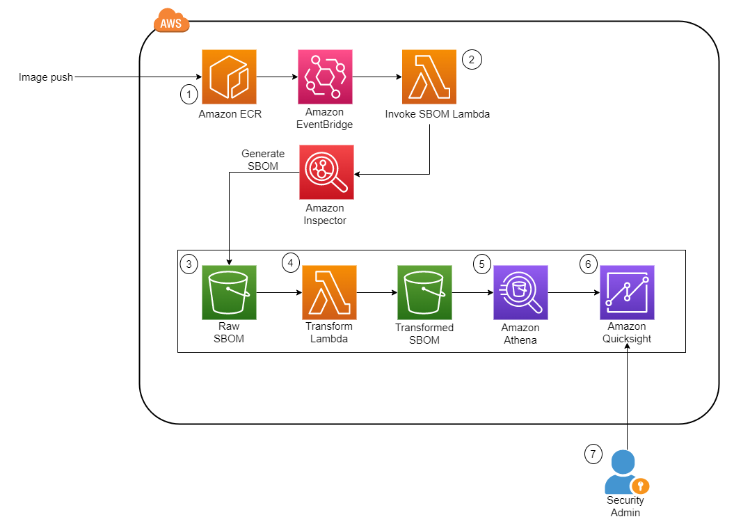
Mansi Bhutada is an ISV Solutions Architect based in the Netherlands. She helps customers design and implement well-architected solutions in AWS that address their business problems. She is passionate about data analytics and networking. Beyond work, she enjoys experimenting with food, playing pickleball, and diving into fun board games.

Hernan Garcia is a Senior Solutions Architect at AWS based in the Netherlands. He works in the financial services industry, supporting enterprises in their cloud adoption. He is passionate about serverless technologies, security, and compliance. He enjoys spending time with family and friends, and trying out new dishes from different cuisines.

The Open Collective Foundation is shutting down

Post Syndicated from corbet original https://lwn.net/Articles/963958/

The Open Collective
Foundation
is an organization created to provide legal and financial
services for non-profit projects, many of which are associated with free
software. Projects hosted there are now beginning
to report
that the Open Collective Foundation will be shutting down at
the end of the year, with an unwinding process over that time.

Unfortunately, over the past year, we have learned that Open
Collective Foundation’s business model is not sustainable with the
number of complex services we have offered and the fees we pay to
the Open Collective Inc. tech platform.

In late 2023, we made the decision to pause accepting new
collectives in order to create space for us to address the
issues. Unfortunately, it became clear that it would not be
financially feasible to make the necessary corrections, and we
determined that OCF is not viable.

Some more information can be found in the Dissolution FAQ. Note
that the Open Collective Foundation is distinct from Open Source Collective, which has hastened
to point out
that it remains in operation as before, and both are
distinct from the Open Collective
platform.

Open sourcing Pingora: our Rust framework for building programmable network services

Post Syndicated from Yuchen Wu original https://blog.cloudflare.com/pingora-open-source


Today, we are proud to open source Pingora, the Rust framework we have been using to build services that power a significant portion of the traffic on Cloudflare. Pingora is released under the Apache License version 2.0.

As mentioned in our previous blog post, Pingora is a Rust async multithreaded framework that assists us in constructing HTTP proxy services. Since our last blog post, Pingora has handled nearly a quadrillion Internet requests across our global network.

We are open sourcing Pingora to help build a better and more secure Internet beyond our own infrastructure. We want to provide tools, ideas, and inspiration to our customers, users, and others to build their own Internet infrastructure using a memory safe framework. Having such a framework is especially crucial given the increasing awareness of the importance of memory safety across the industry and the US government. Under this common goal, we are collaborating with the Internet Security Research Group (ISRG) Prossimo project to help advance the adoption of Pingora in the Internet’s most critical infrastructure.

In our previous blog post, we discussed why and how we built Pingora. In this one, we will talk about why and how you might use Pingora.

Pingora provides building blocks for not only proxies but also clients and servers. Along with these components, we also provide a few utility libraries that implement common logic such as event counting, error handling, and caching.

What’s in the box

Pingora provides libraries and APIs to build services on top of HTTP/1 and HTTP/2, TLS, or just TCP/UDP. As a proxy, it supports HTTP/1 and HTTP/2 end-to-end, gRPC, and websocket proxying. (HTTP/3 support is on the roadmap.) It also comes with customizable load balancing and failover strategies. For compliance and security, it supports both the commonly used OpenSSL and BoringSSL libraries, which come with FIPS compliance and post-quantum crypto.

Besides providing these features, Pingora provides filters and callbacks to allow its users to fully customize how the service should process, transform and forward the requests. These APIs will be especially familiar to OpenResty and NGINX users, as many map intuitively onto OpenResty’s “*_by_lua” callbacks.

Operationally, Pingora provides zero downtime graceful restarts to upgrade itself without dropping a single incoming request. Syslog, Prometheus, Sentry, OpenTelemetry and other must-have observability tools are also easily integrated with Pingora as well.

Who can benefit from Pingora

You should consider Pingora if:

Security is your top priority: Pingora is a more memory safe alternative for services that are written in C/C++. While some might argue about memory safety among programming languages, from our practical experience, we find ourselves way less likely to make coding mistakes that lead to memory safety issues. Besides, as we spend less time struggling with these issues, we are more productive implementing new features.

Your service is performance-sensitive: Pingora is fast and efficient. As explained in our previous blog post, we saved a lot of CPU and memory resources thanks to Pingora’s multi-threaded architecture. The saving in time and resources could be compelling for workloads that are sensitive to the cost and/or the speed of the system.

Your service requires extensive customization: The APIs that the Pingora proxy framework provides are highly programmable. For users who wish to build a customized and advanced gateway or load balancer, Pingora provides powerful yet simple ways to implement it. We provide examples in the next section.

Let’s build a load balancer

Let’s explore Pingora’s programmable API by building a simple load balancer. The load balancer will select between https://1.1.1.1/ and https://1.0.0.1/ to be the upstream in a round-robin fashion.

First let’s create a blank HTTP proxy.

pub struct LB();

#[async_trait]
impl ProxyHttp for LB {
    async fn upstream_peer(...) -> Result<Box<HttpPeer>> {
        todo!()
    }
}

Any object that implements the ProxyHttp trait (similar to the concept of an interface in C++ or Java) is an HTTP proxy. The only required method there is upstream_peer(), which is called for every request. This function should return an HttpPeer which contains the origin IP to connect to and how to connect to it.

Next let’s implement the round-robin selection. The Pingora framework already provides the LoadBalancer with common selection algorithms such as round robin and hashing, so let’s just use it. If the use case requires more sophisticated or customized server selection logic, users can simply implement it themselves in this function.

pub struct LB(Arc<LoadBalancer<RoundRobin>>);

#[async_trait]
impl ProxyHttp for LB {
    async fn upstream_peer(...) -> Result<Box<HttpPeer>> {
        let upstream = self.0
            .select(b"", 256) // hash doesn't matter for round robin
            .unwrap();

        // Set SNI to one.one.one.one
        let peer = Box::new(HttpPeer::new(upstream, true, "one.one.one.one".to_string()));
        Ok(peer)
    }
}

Since we are connecting to an HTTPS server, the SNI also needs to be set. Certificates, timeouts, and other connection options can also be set here in the HttpPeer object if needed.

Finally, let’s put the service in action. In this example we hardcode the origin server IPs. In real life workloads, the origin server IPs can also be discovered dynamically when the upstream_peer() is called or in the background. After the service is created, we just tell the LB service to listen to 127.0.0.1:6188. In the end we created a Pingora server, and the server will be the process which runs the load balancing service.

fn main() {
    let mut upstreams = LoadBalancer::try_from_iter(["1.1.1.1:443", "1.0.0.1:443"]).unwrap();

    let mut lb = pingora_proxy::http_proxy_service(&my_server.configuration, LB(upstreams));
    lb.add_tcp("127.0.0.1:6188");

    let mut my_server = Server::new(None).unwrap();
    my_server.add_service(lb);
    my_server.run_forever();
}

Let’s try it out:

curl 127.0.0.1:6188 -svo /dev/null
> GET / HTTP/1.1
> Host: 127.0.0.1:6188
> User-Agent: curl/7.88.1
> Accept: */*
> 
< HTTP/1.1 403 Forbidden

We can see that the proxy is working, but the origin server rejects us with a 403. This is because our service simply proxies the Host header, 127.0.0.1:6188, set by curl, which upsets the origin server. How do we make the proxy correct that? This can simply be done by adding another filter called upstream_request_filter. This filter runs on every request after the origin server is connected and before any HTTP request is sent. We can add, remove or change http request headers in this filter.

async fn upstream_request_filter(…, upstream_request: &mut RequestHeader, …) -> Result<()> {
    upstream_request.insert_header("Host", "one.one.one.one")
}

Let’s try again:

curl 127.0.0.1:6188 -svo /dev/null
< HTTP/1.1 200 OK

This time it works! The complete example can be found here.

Below is a very simple diagram of how this request flows through the callback and filter we used in this example. The Pingora proxy framework currently provides more filters and callbacks at different stages of a request to allow users to modify, reject, route and/or log the request (and response).

Behind the scenes, the Pingora proxy framework takes care of connection pooling, TLS handshakes, reading, writing, parsing requests and any other common proxy tasks so that users can focus on logic that matters to them.

Open source, present and future

Pingora is a library and toolset, not an executable binary. In other words, Pingora is the engine that powers a car, not the car itself. Although Pingora is production-ready for industry use, we understand a lot of folks want a batteries-included, ready-to-go web service with low or no-code config options. Building that application on top of Pingora will be the focus of our collaboration with the ISRG to expand Pingora’s reach. Stay tuned for future announcements on that project.

Other caveats to keep in mind:

  • Today, API stability is not guaranteed. Although we will try to minimize how often we make breaking changes, we still reserve the right to add, remove, or change components such as request and response filters as the library evolves, especially during this pre-1.0 period.
  • Support for non-Unix based operating systems is not currently on the roadmap. We have no immediate plans to support these systems, though this could change in the future.

How to contribute

Feel free to raise bug reports, documentation issues, or feature requests in our GitHub issue tracker. Before opening a pull request, we strongly suggest you take a look at our contribution guide.

Conclusion

In this blog we announced the open source of our Pingora framework. We showed that Internet entities and infrastructure can benefit from Pingora’s security, performance and customizability. We also demonstrated how easy it is to use Pingora and how customizable it is.

Whether you’re building production web services or experimenting with network technologies we hope you find value in Pingora. It’s been a long journey, but sharing this project with the open source community has been a goal from the start. We’d like to thank the Rust community as Pingora is built with many great open-sourced Rust crates. Moving to a memory safe Internet may feel like an impossible journey, but it’s one we hope you join us on.

Security updates for Wednesday

Post Syndicated from jzb original https://lwn.net/Articles/963957/

Security updates have been issued by Debian (knot-resolver and wpa), Fedora (chromium, kernel, thunderbird, and yarnpkg), Mageia (c-ares), Oracle (firefox, kernel, opensc, postgresql:13, postgresql:15, and thunderbird), Red Hat (edk2, gimp:2.8, and kernel), SUSE (bind, bluez, container-suseconnect, dnsdist, freerdp, gcc12, gcc7, glib2, gnutls, kernel, kubevirt, virt-api-container, virt-controller-container, virt-exportproxy-container, virt-exportserver-container, virt-handler-container, virt-launcher-container, virt-libguestfs-t, libqt5-qtbase, libqt5-qtsvg, nodejs18, nodejs20, openssl, openssl-1_0_0, poppler, python-crcmod, python-cryptography, python-cryptography- vectors, python-pip, python-requests, python3-requests, python311, python39, rabbitmq-c, samba, sccache, shim, SUSE Manager 4.2, SUSE Manager Server 4.2, the Linux-RT Kernel, and thunderbird), and Ubuntu (less, openssl, php7.0, php7.2, php7.4, and tiff).

How to develop an Amazon Security Lake POC

Post Syndicated from Anna McAbee original https://aws.amazon.com/blogs/security/how-to-develop-an-amazon-security-lake-poc/

You can use Amazon Security Lake to simplify log data collection and retention for Amazon Web Services (AWS) and non-AWS data sources. To make sure that you get the most out of your implementation requires proper planning.

In this post, we will show you how to plan and implement a proof of concept (POC) for Security Lake to help you determine the functionality and value of Security Lake in your environment, so that your team can confidently design and implement in production. We will walk you through the following steps:

  1. Understand the functionality and value of Security Lake
  2. Determine success criteria for the POC
  3. Define your Security Lake configuration
  4. Prepare for deployment
  5. Enable Security Lake
  6. Validate deployment

Understand the functionality of Security Lake

Figure 1 summarizes the main features of Security Lake and the context of how to use it:

Figure 1: Overview of Security Lake functionality

Figure 1: Overview of Security Lake functionality

As shown in the figure, Security Lake ingests and normalizes logs from data sources such as AWS services, AWS Partner sources, and custom sources. Security Lake also manages the lifecycle, orchestration, and subscribers. Subscribers can be AWS services, such as Amazon Athena, or AWS Partner subscribers.

There are four primary functions that Security Lake provides:

  • Centralize visibility to your data from AWS environments, SaaS providers, on-premises, and other cloud data sources — You can collect log sources from AWS services such as AWS CloudTrail management events, Amazon Simple Storage Service (Amazon S3) data events, AWS Lambda data events, Amazon Route 53 Resolver logs, VPC Flow Logs, and AWS Security Hub findings, in addition to log sources from on-premises, other cloud services, SaaS applications, and custom sources. Security Lake automatically aggregates the security data across AWS Regions and accounts.
  • Normalize your security data to an open standard — Security Lake normalizes log sources in a common schema, the Open Security Schema Framework (OCSF), and stores them in compressed parquet files.
  • Use your preferred analytics tools to analyze your security data — You can use AWS tools, such as Athena and Amazon OpenSearch Service, or you can utilize external security tools to analyze the data in Security Lake.
  • Optimize and manage your security data for more efficient storage and query — Security Lake manages the lifecycle of your data with customizable retention settings with automated storage tiering to help provide more cost-effective storage.

Determine success criteria

By establishing success criteria, you can assess whether Security Lake has helped address the challenges that you are facing. Some example success criteria include:

  • I need to centrally set up and store AWS logs across my organization in AWS Organizations for multiple log sources.
  • I need to more efficiently collect VPC Flow Logs in my organization and analyze them in my security information and event management (SIEM) solution.
  • I want to use OpenSearch Service to replace my on-premises SIEM.
  • I want to collect AWS log sources and custom sources for machine learning with Amazon Sagemaker.
  • I need to establish a dashboard in Amazon QuickSight to visualize my Security Hub findings and a custom log source data.

Review your success criteria to make sure that your goals are realistic given your timeframe and potential constraints that are specific to your organization. For example, do you have full control over the creation of AWS services that are deployed in an organization? Do you have resources that can dedicate time to implement and test? Is this time convenient for relevant stakeholders to evaluate the service?

The timeframe of your POC will depend on your answers to these questions.

Important: Security Lake has a 15-day free trial per account that you use from the time that you enable Security Lake. This is the best way to estimate the costs for each Region throughout the trial, which is an important consideration when you configure your POC.

Define your Security Lake configuration

After you establish your success criteria, you should define your desired Security Lake configuration. Some important decisions include the following:

  • Determine AWS log sources — Decide which AWS log sources to collect. For information about the available options, see Collecting data from AWS services.
  • Determine third-party log sources — Decide if you want to include non-AWS service logs as sources in your POC. For more information about your options, see Third-party integrations with Security Lake; the integrations listed as “Source” can send logs to Security Lake.

    Note: You can add third-party integrations after the POC or in a second phase of the POC. Pre-planning will be required to make sure that you can get these set up during the 15-day free trial. Third-party integrations usually take more time to set up than AWS service logs.

  • Select a delegated administrator – Identify which account will serve as the delegated administrator. Make sure that you have the appropriate permissions from the organization admin account to identify and enable the account that will be your Security Lake delegated administrator. This account will be the location for the S3 buckets with your security data and where you centrally configure Security Lake. The AWS Security Reference Architecture (AWS SRA) recommends that you use the AWS logging account for this purpose. In addition, make sure to review Important considerations for delegated Security Lake administrators.
  • Select accounts in scope — Define which accounts to collect data from. To get the most realistic estimate of the cost of Security Lake, enable all accounts across your organization during the free trial.
  • Determine analytics tool — Determine if you want to use native AWS analytics tools, such as Athena and OpenSearch Service, or an existing SIEM, where the SIEM is a subscriber to Security Lake.
  • Define log retention and Regions — Define your log retention requirements and Regional restrictions or considerations.

Prepare for deployment

After you determine your success criteria and your Security Lake configuration, you should have an idea of your stakeholders, desired state, and timeframe. Now you need to prepare for deployment. In this step, you should complete as much as possible before you deploy Security Lake. The following are some steps to take:

  • Create a project plan and timeline so that everyone involved understands what success look like and what the scope and timeline is.
  • Define the relevant stakeholders and consumers of the Security Lake data. Some common stakeholders include security operations center (SOC) analysts, incident responders, security engineers, cloud engineers, finance, and others.
  • Define who is responsible, accountable, consulted, and informed during the deployment. Make sure that team members understand their roles.
  • Make sure that you have access in your management account to delegate and administrator. For further details, see IAM permissions required to designate the delegated administrator.
  • Consider other technical prerequisites that you need to accomplish. For example, if you need roles in addition to what Security Lake creates for custom extract, transform, and load (ETL) pipelines for custom sources, can you work with the team in charge of that process before the POC?

Enable Security Lake

The next step is to enable Security Lake in your environment and configure your sources and subscribers.

  1. Deploy Security Lake across the Regions, accounts, and AWS log sources that you previously defined.
  2. Configure custom sources that are in scope for your POC.
  3. Configure analytics tools in scope for your POC.

Validate deployment

The final step is to confirm that you have configured Security Lake and additional components, validate that everything is working as intended, and evaluate the solution against your success criteria.

  • Validate log collection — Verify that you are collecting the log sources that you configured. To do this, check the S3 buckets in the delegated administrator account for the logs.
  • Validate analytics tool — Verify that you can analyze the log sources in your analytics tool of choice. If you don’t want to configure additional analytics tooling, you can use Athena, which is configured when you set up Security Lake. For sample Athena queries, see Amazon Security Lake Example Queries on GitHub and Security Lake queries in the documentation.
  • Obtain a cost estimate — In the Security Lake console, you can review a usage page to verify that the cost of Security Lake in your environment aligns with your expectations and budgets.
  • Assess success criteria — Determine if you achieved the success criteria that you defined at the beginning of the project.

Next steps

Next steps will largely depend on whether you decide to move forward with Security Lake.

  • Determine if you have the approval and budget to use Security Lake.
  • Expand to other data sources that can help you provide more security outcomes for your business.
  • Configure S3 lifecycle policies to efficiently store logs long term based on your requirements.
  • Let other teams know that they can subscribe to Security Lake to use the log data for their own purposes. For example, a development team that gets access to CloudTrail through Security Lake can analyze the logs to understand the permissions needed for an application.

Conclusion

In this blog post, we showed you how to plan and implement a Security Lake POC. You learned how to do so through phases, including defining success criteria, configuring Security Lake, and validating that Security Lake meets your business needs.

As a customer, this guide will help you run a successful proof of value (POV) with Security Lake. It guides you in assessing the value and factors to consider when deciding to implement the current features.

Further resources

 
If you have feedback about this post, submit comments in the Comments section below. If you have questions about this post, contact AWS Support.

Anna McAbee

Anna McAbee

Anna is a Security Specialist Solutions Architect focused on threat detection and incident response at AWS. Before AWS, she worked as an AWS customer in financial services on both the offensive and defensive sides of security. Outside of work, Anna enjoys cheering on the Florida Gators football team, wine tasting, and traveling the world.

Author

Marshall Jones

Marshall is a Worldwide Security Specialist Solutions Architect at AWS. His background is in AWS consulting and security architecture, focused on a variety of security domains including edge, threat detection, and compliance. Today, he is focused on helping enterprise AWS customers adopt and operationalize AWS security services to increase security effectiveness and reduce risk.

Marc Luescher

Marc Luescher

Marc is a Senior Solutions Architect helping enterprise customers be successful, focusing strongly on threat detection, incident response, and data protection. His background is in networking, security, and observability. Previously, he worked in technical architecture and security hands-on positions within the healthcare sector as an AWS customer. Outside of work, Marc enjoys his 3 dogs, 4 cats, and 20+ chickens.