Since Amazon Aurora launched in 2014, hundreds of thousands of customers have chosen Aurora to run their most demanding applications. Aurora provides unparalleled high performance and availability at global scale with full MySQL and PostgreSQL compatibility at up to one-tenth the cost of commercial databases.
Many customers benefit from the cost-effectiveness of Aurora’s current simple, pay-per-request pricing for input/output (I/O) usage, removing the need to provision I/Os in advance. Customers also benefit from additional cost-saving innovations such as Amazon Aurora Serverless v2 (ASv2), which provides seamless scaling in fine-grained increments based on the application’s demands. For workloads with spikes in demand, you can save up to 90 percent in costs vs. provisioning capacity for peak load with ASv2.
Today, we are announcing the general availability of Amazon Aurora I/O-Optimized, a new cluster configuration that offers improved price performance and predictable pricing for customers with I/O-intensive applications, such as e-commerce applications, payment processing systems, and more. Aurora I/O-Optimized offers improved performance, increasing throughput and reducing latency to support your most demanding workloads.
You can now confidently predict costs for your most I/O-intensive workloads, with up to 40 percent cost savings when your I/O spend exceeds 25 percent of your current Aurora database spend. If you are using Reserved Instances, you will see even greater cost savings.
Now you have the flexibility to choose between the existing configuration newly called Aurora Standard, which is the existing pay-per-request pricing model that is cost-effective for applications with low-to-moderate I/O usage or the new Aurora I/O-Optimized configuration for I/O-intensive applications.
Getting Started with Aurora I/O-Optimized You can create a new database cluster using the Aurora I/O-Optimized configuration or convert your existing database clusters with a few clicks in the AWS Management Console, AWS Command Line Interface (AWS CLI), or AWS SDKs.
For the Aurora MySQL-Compatible Edition and Aurora PostgreSQL-Compatible Edition, you can choose either the Aurora Standard or Aurora I/O-Optimized configuration.
Aurora I/O-Optimized configuration is available in the latest version of Aurora MySQL version 3.03.1 and higher, Aurora PostgreSQL v15.2 and higher, v14.7 and higher, and v13.10 and higher.
This configuration supports Intel-based Aurora database instance types such as t3, r5, and r6i, Graviton-based database instance types such as t4g, r7g, and x2g, Aurora Serverless v2, Aurora Global Database, on-demand Aurora database instances, and reserved instances.
R7g instances for Amazon Aurora are powered by the latest generation AWS Graviton3 processors, delivering up to 30 percent performance gains and up to 20 percent improved price performance for Aurora, as compared to R6g instances.
In your existing Aurora clusters, you can switch the storage configuration to Aurora I/O-Optimized once every 30 days or switch back to Aurora Standard at any time. You can change the cluster storage configuration only at the cluster level. The change applies to all instances in the cluster.
After changing the configuration, you don’t need to reboot the database instances within the cluster to take advantage of the price-performance benefits of Aurora I/O-Optimized.
Now Available Amazon Aurora I/O-Optimized configuration is now generally available for Amazon Aurora MySQL-Compatible Edition and Aurora PostgreSQL-Compatible Edition in most AWS Regions where Aurora is available, with China (Beijing), China (Ningxia), AWS GovCloud (US-East), and AWS GovCloud (US-West) Regions coming soon.
Aurora is billed differently for the two configurations: Aurora Standard or Aurora I/O-Optimized. The latter doesn’t charge for I/Os, charging a set price for compute and storage relative to the former. For I/O-intensive applications, its price/performance will be better, and you can save up to 40 percent on costs. To see pricing examples, visit the Aurora Pricing page.
A new week starts, and Spring is almost here! If you’re curious about AWS news from the previous seven days, I got you covered.
Last Week’s Launches Here are the launches that got my attention last week:
Amazon S3 – Last week there was AWS Pi Day 2023 celebrating 17 years of innovation since Amazon S3 was introduced on March 14, 2006. For the occasion, the team released many new capabilities:
Amazon S3 has also simplified private connectivity from on-premises networks: with private DNS for S3, on-premises applications can use AWS PrivateLink to access S3 over an interface endpoint, while requests from your in-VPC applications access S3 using gateway endpoints.
We released Mountpoint for Amazon S3, a high performance open source file client. Read more in the blog. Note that Mountpoint isn’t a general-purpose networked file system, and comes with some restrictions on file operations.
Amazon Neptune – Now offers a graph summary API to help understand important metadata about property graphs (PG) and resource description framework (RDF) graphs. Neptune added support for Slow Query Logs to help identify queries that need performance tuning.
Amazon OpenSearch Service – The team introduced security analytics that provides new threat monitoring, detection, and alerting features. The service now supports OpenSearchversion 2.5 that adds several new features such as support for Point in Time Search and improvements to observability and geospatial functionality.
AWS Lake Formation and Apache Hive on Amazon EMR – Introduced fine-grained access controls that allow data administrators to define and enforce fine-grained table and column level security for customers accessing data via Apache Hive running on Amazon EMR.
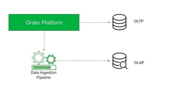
When we talk with customers, we hear that they want to be able to harness insights from data in order to make timely, impactful, and actionable business decisions. A common pattern with data-driven organizations is that they have many different data sources they need to ingest into their analytics systems. This requires them to build manual data pipelines spanning across their operational databases, data lakes, streaming data, and data within their warehouse. As a consequence of this complex setup, it can take data engineers weeks or even months to build data ingestion pipelines. These data pipelines are costly, and the delays can lead to missed business opportunities. Additionally, data warehouses are increasingly becoming mission critical systems that require high availability, reliability, and security.
Amazon Redshift is a fully managed petabyte-scale data warehouse used by tens of thousands of customers to easily, quickly, securely, and cost-effectively analyze all their data at any scale. This year at re:Invent, Amazon Redshift has announced a number of features to help you simplify data ingestion and get to insights easily and quickly, within a secure, reliable environment.
In this blog, I introduce some of these new features that fit into two main categories:
Simplify data ingestion
Amazon Redshift now supports auto-copy from Amazon S3 (available in preview). With this new capability, Amazon Redshift automatically loads the files that arrive in an Amazon Simple Storage Service (Amazon S3) location that you specify into your data warehouse. The files can use any of the formats supported by the Amazon Redshift copy command, such as CSV, JSON, Parquet, and Avro. In this way, you don’t need to manually or repeatedly run copy procedures. Amazon Redshift automates file ingestion and takes care of data-loading steps under the hood.
With Amazon Aurora zero-ETL integration with Amazon Redshift, you can use Amazon Redshift for near real-time analytics and machine learning on petabytes of transactional data stored on Amazon Aurora MySQL databases (available in limited preview). With this capability, you can choose the Amazon Aurora databases containing the data you want to analyze with Amazon Redshift. Data is then replicated into your data warehouse within seconds after transactional data is written into Amazon Aurora, eliminating the need to build and maintain complex data pipelines. You can replicate data from multiple Amazon Aurora databases into the same Amazon Redshift instance to run analytics across multiple applications. With near real-time access to transactional data, you can leverage Amazon Redshift’s analytics and capabilities, such as built-in machine learning (ML), materialized views, data sharing, and federated access to multiple data stores and data lakes, to derive insights from transactional and other data.
With the general availability of Amazon Redshift Streaming Ingestion, you can now natively ingest hundreds of megabytes of data per second from Amazon Kinesis Data Streams and Amazon MSK into an Amazon Redshift materialized view and query it in seconds. Learn more in this post.
Make your data warehouse more secure and reliable
You can now improve the availability of your data warehouse by choosing multiple Availability Zone (AZ) deployments. Multi-AZ deployments for your Amazon Redshift clusters are available in preview and reduce recovery times to seconds through automatic recovery. In this way, you can build solutions that are more compliant with the recommendations of the Reliability Pillar of the AWS Well-Architected Framework.
With dynamic data masking (available in preview), you can protect sensitive information stored in your data warehouse and ensure that only the relevant data is accessible by users based on their roles. You can limit how much identifiable data is visible to users using multiple levels of policies so different users and groups can have different levels of data access without having to create multiple copies of data. Dynamic data masking complements other granular access control capabilities in Amazon Redshift including row-level and column-level security and role-based access controls. In this way, Dynamic Data Masking helps you meet requirements for GDPR, CCPA, and other privacy regulations.
Amazon Redshift now supports central access controls for data sharing with AWS Lake Formation (available in public preview). You can now use Lake Formation to simplify governance of data shared from Amazon Redshift and centrally manage granular access across all data-sharing consumers.
There have been other interesting news for Amazon Redshift at re:Invent you might have already heard about:
The general availability of Amazon Redshift integration for Apache Spark makes it easy to build and run Spark applications on Amazon Redshift and Redshift Serverless, opening up the data warehouse for a broader set of AWS analytics and machine learning solutions.
AWS Backup now supports Amazon Redshift. AWS Backup allows you to define a central backup policy to manage data protection of your applications and can also protect your Amazon Redshift clusters. In this way, you have a consistent experience when managing data protection across all supported services.
Availability and Pricing Multi-AZ deployments, central access control for data sharing with AWS Lake Formation, auto-copy from Amazon S3, and dynamic data masking are available in preview in US East (Ohio), US East (N. Virginia), US West (Oregon), Asia Pacific (Tokyo), Europe (Ireland), and Europe (Stockholm).
There is no additional cost for using auto-copy from Amazon S3 and near real-time analytics on transactional data. There is no extra charge for dynamic data masking and central access control for data sharing. For more information, see Amazon Redshift pricing.
These new capabilities take you one step further in analyzing all your data across data sources with simple data ingestion capabilities, while improving the security and reliability of your data warehouse.
Amazon DocumentDB (with MongoDB compatibility) is a scalable, highly durable, and fully managed database service for operating mission-critical JSON workloads. It is one of AWS fast-growing services with customers including BBC, Dow Jones, and Samsung relying on Amazon DocumentDB to run their JSON workloads at scale.
Today I am excited to announce the general availability of Amazon DocumentDB Elastic Clusters. Elastic Clusters enables you to elastically scale your document database to handle virtually any number of writes and reads, with petabytes of storage capacity. Elastic Clusters simplifies how customers interact with Amazon DocumentDB by automatically managing the underlying infrastructure and removing the need to create, remove, upgrade, or scale instances.
A Few Concepts about Elastic Clusters Sharding – A popular database concept also known as partitioning, sharding splits large data sets into smaller data sets across multiple nodes enabling customers to scale out their database beyond vertical scaling limits. Elastic Clusters uses sharding to partition data across Amazon DocumentDB’s distributed storage system.
Elastic Clusters – Elastic Clusters is Amazon DocumentDB clusters that allow you to scale your workload’s throughput to millions of writes/reads per second and storage to petabytes. Elastic Clusters comprises one or more shards each of which has its own compute and storage volume. It is highly available across three Availability Zones (AZs) by default, with six copies of your data replicated across these three AZs. You can create Elastic Clusters using the Amazon DocumentDB API, AWS SDK, AWS CLI, AWS CloudFormation, or the AWS console.
Scale Workloads with Little to No Impact – With Elastic Clusters, your database can scale to millions of operations with little to no downtime or performance impact.
Getting Started with Elastic Clusters Previously, I mentioned that you can use either the AWS console, AWS CLI, or AWS SDK to create Elastic Clusters. In the examples below, we will look at how you can create a cluster, scale up or out, and scale in or down using the AWS CLI:
Create a Cluster When creating a cluster, you will specify the vCPUs that you want for your Elastic Clusters at provisioning. With the size of vCPUs that you provision, you will also get a proportionate amount of memory, expressed in vCPUs. Elastic Clusters automatically provisions the necessary infrastructure (shards and instances) on your behalf. aws docdb-elastic create-cluster --cluster-name foo --shard-capacity 2 --shard-count 4 --auth-type PLAIN_TEXT --admin-user-name docdbelasticadmin --admin-user-password password
Scale Up or Out If you need more compute and storage to handle an increase in traffic, modify the shard-count parameter. Elastic Clusters scales the underlying infrastructure up or out to give you additional compute and storage capacity. aws docdb-elastic update-cluster --cluster-arn foo-arn --shard-count 8
Scale In or Down If you no longer need the compute and storage that you currently have provisioned, either due to a decline in database traffic or the fact that you originally over-provisioned, modify the shard-count parameter. Elastic Clusters scales the underlying infrastructure in or down. aws docdb-elastic update-cluster --cluster-arn foo-arn --shard-count 4
General Availability of Elastic Clusters for Amazon DocumentDB Amazon DocumentDB Elastic Clusters is now available in all AWS Regions where Amazon DocumentDB is available, except China and AWS GovCloud. To learn more, visit the Amazon DocumentDB page.
Ten years ago, just a few months after I joined AWS, Amazon Redshift was launched. Over the years, many features have been added to improve performance and make it easier to use. Amazon Redshift now allows you to analyze structured and semi-structured data across data warehouses, operational databases, and data lakes. More recently, Amazon Redshift Serverless became generally available to make it easier to run and scale analytics without having to manage your data warehouse infrastructure.
To process data as quickly as possible from real-time applications, customers are adopting streaming engines like Amazon Kinesis and Amazon Managed Streaming for Apache Kafka. Previously, to load streaming data into your Amazon Redshift database, you’d have to configure a process to stage data in Amazon Simple Storage Service (Amazon S3) before loading. Doing so would introduce a latency of one minute or more, depending on the volume of data.
Today, I am happy to share the general availability of Amazon Redshift Streaming Ingestion. With this new capability, Amazon Redshift can natively ingest hundreds of megabytes of data per second from Amazon Kinesis Data Streams and Amazon MSK into an Amazon Redshift materialized view and query it in seconds.
Streaming ingestion benefits from the ability to optimize query performance with materialized views and allows the use of Amazon Redshift more efficiently for operational analytics and as the data source for real-time dashboards. Another interesting use case for streaming ingestion is analyzing real-time data from gamers to optimize their gaming experience. This new integration also makes it easier to implement analytics for IoT devices, clickstream analysis, application monitoring, fraud detection, and live leaderboards.
Let’s see how this works in practice.
Configuring Amazon Redshift Streaming Ingestion Apart from managing permissions, Amazon Redshift streaming ingestion can be configured entirely with SQL within Amazon Redshift. This is especially useful for business users who lack access to the AWS Management Console or the expertise to configure integrations between AWS services.
You can set up streaming ingestion in three steps:
Create or update an AWS Identity and Access Management (IAM) role to allow access to the streaming platform you use (Kinesis Data Streams or Amazon MSK). Note that the IAM role should have a trust policy that allows Amazon Redshift to assume the role.
Create an external schema to connect to the streaming service.
Create a materialized view that references the streaming object (Kinesis data stream or Kafka topic) in the external schemas.
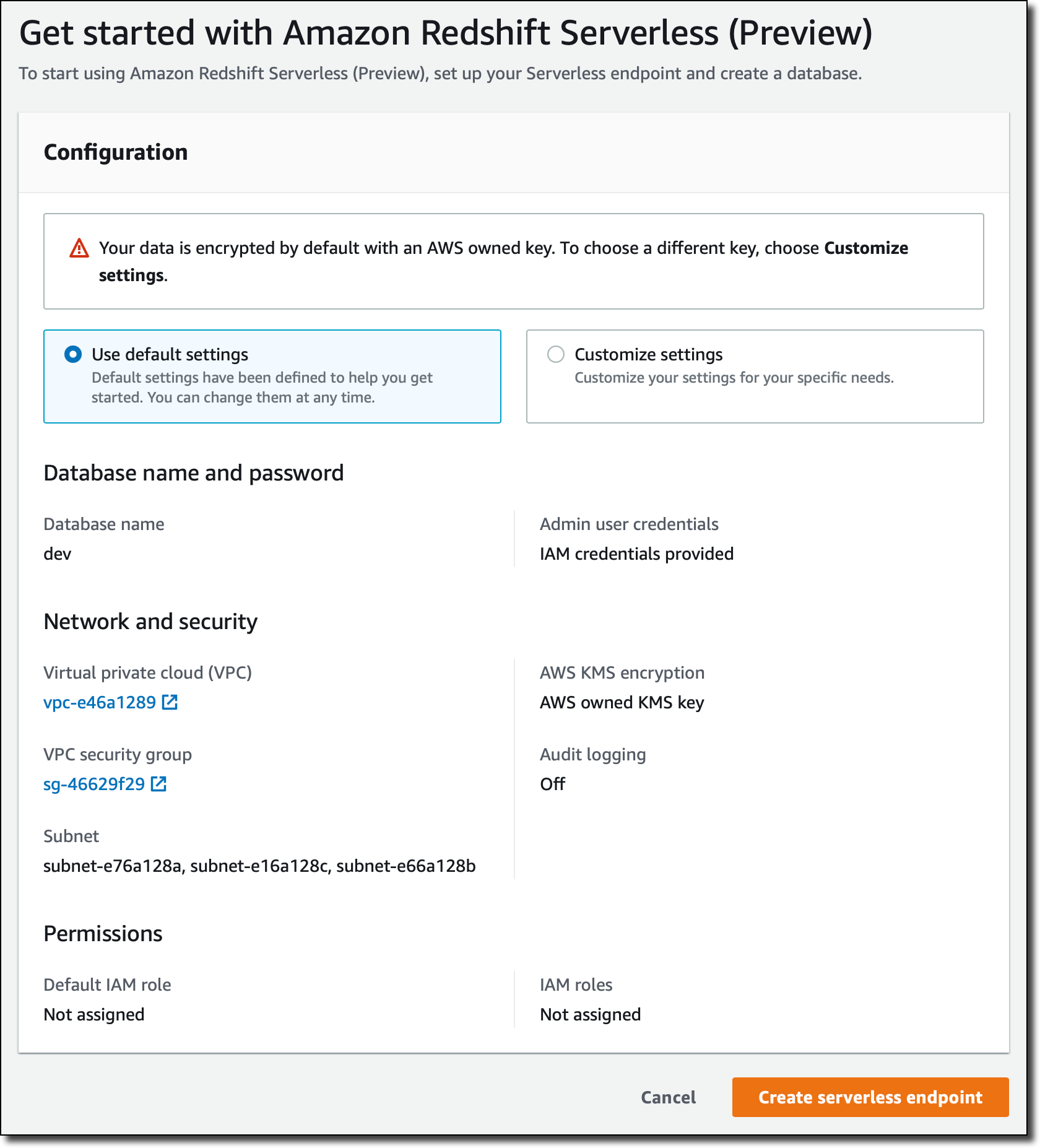
After that, you can query the materialized view to use the data from the stream in your analytics workloads. Streaming ingestion works with Amazon Redshift provisioned clusters and with the new serverless option. To maximize simplicity, I am going to use Amazon Redshift Serverless in this walkthrough.
To prepare my environment, I need a Kinesis data stream. In the Kinesis console, I choose Data streams in the navigation pane and then Create data stream. For the Data stream name, I use my-input-stream and then leave all other options set to their default value. After a few seconds, the Kinesis data stream is ready. Note that by default I am using on-demand capacity mode. In a development or test environment, you can choose provisioned capacity mode with one shard to optimize costs.
Now, I create an IAM role to give Amazon Redshift access to the my-input-stream Kinesis data streams. In the IAM console, I create a role with this policy:
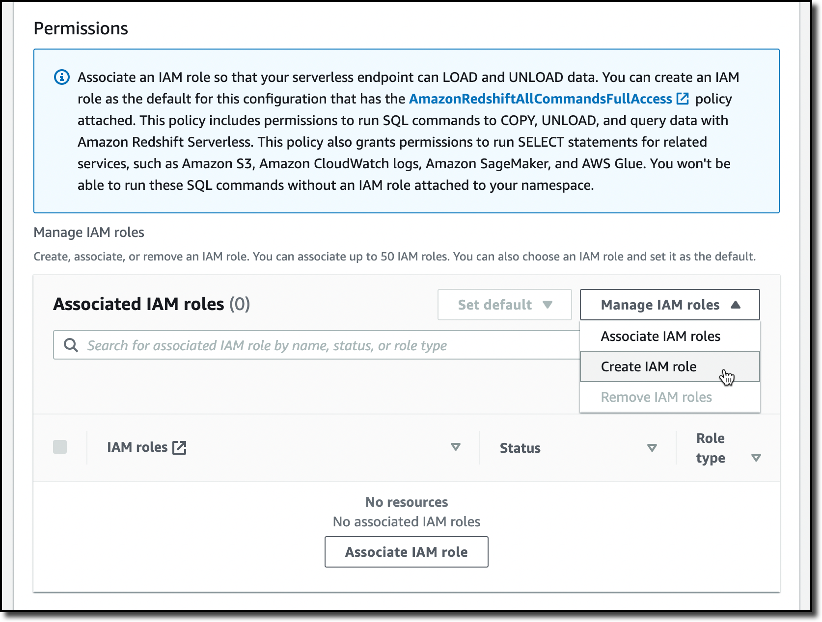
In the Amazon Redshift console, I choose Redshift serverless from the navigation pane and create a new workgroup and namespace, similar to what I did in this blog post. When I create the namespace, in the Permissions section, I choose Associate IAM roles from the dropdown menu. Then, I select the role I just created. Note that the role is visible in this selection only if the trust policy allows Amazon Redshift to assume it. After that, I complete the creation of the namespace using the default options. After a few minutes, the serverless database is ready for use.
In the Amazon Redshift console, I choose Query editor v2 in the navigation pane. I connect to the new serverless database by choosing it from the list of resources. Now, I can use SQL to configure streaming ingestion. First, I create an external schema that maps to the streaming service. Because I am going to use simulated IoT data as an example, I call the external schema sensors.
CREATE EXTERNAL SCHEMA sensors
FROM KINESIS
IAM_ROLE 'arn:aws:iam::123412341234:role/redshift-streaming-ingestion';
To access the data in the stream, I create a materialized view that selects data from the stream. In general, materialized views contain a precomputed result set based on the result of a query. In this case, the query is reading from the stream, and Amazon Redshift is the consumer of the stream.
Because streaming data is going to be ingested as JSON data, I have two options:
Leave all the JSON data in a single column and use Amazon Redshift capabilities to query semi-structured data.
Extract JSON properties into their own separate columns.
Let’s see the pros and cons of both options.
The approximate_arrival_timestamp, partition_key, shard_id, and sequence_number columns in the SELECT statement are provided by Kinesis Data Streams. The record from the stream is in the kinesis_data column. The refresh_time column is provided by Amazon Redshift.
To leave the JSON data in a single column of the sensor_data materialized view, I use the JSON_PARSE function:
CREATE MATERIALIZED VIEW sensor_data AUTO REFRESH YES AS
    SELECT approximate_arrival_timestamp,
           partition_key,
           shard_id,
           sequence_number,
           refresh_time,
           JSON_PARSE(kinesis_data, 'utf-8') as payload
      FROM sensors."my-input-stream";
CREATE MATERIALIZED VIEW sensor_data AUTO REFRESH YES AS
SELECT approximate_arrival_timestamp,
partition_key,
shard_id,
sequence_number,
refresh_time,
JSON_PARSE(kinesis_data) as payload
FROM sensors."my-input-stream";
Because I used the AUTO REFRESH YES parameter, the content of the materialized view is automatically refreshed when there is new data in the stream.
To extract the JSON properties into separate columns of the sensor_data_extract materialized view, I use the JSON_EXTRACT_PATH_TEXT function:
CREATE MATERIALIZED VIEW sensor_data_extract AUTO REFRESH YES AS
    SELECT approximate_arrival_timestamp,
           partition_key,
           shard_id,
           sequence_number,
           refresh_time,
           JSON_EXTRACT_PATH_TEXT(FROM_VARBYTE(kinesis_data, 'utf-8'),'sensor_id')::VARCHAR(8) as sensor_id,
           JSON_EXTRACT_PATH_TEXT(FROM_VARBYTE(kinesis_data, 'utf-8'),'current_temperature')::DECIMAL(10,2) as current_temperature,
           JSON_EXTRACT_PATH_TEXT(FROM_VARBYTE(kinesis_data, 'utf-8'),'status')::VARCHAR(8) as status,
           JSON_EXTRACT_PATH_TEXT(FROM_VARBYTE(kinesis_data, 'utf-8'),'event_time')::CHARACTER(26) as event_time
      FROM sensors."my-input-stream";
Loading Data into the Kinesis Data Stream To put data in the my-input-stream Kinesis Data Stream, I use the following random_data_generator.py Python script simulating data from IoT sensors:
import datetime
import json
import random
import boto3

STREAM_NAME = "my-input-stream"


def get_random_data():
    current_temperature = round(10 + random.random() * 170, 2)
    if current_temperature > 160:
        status = "ERROR"
    elif current_temperature > 140 or random.randrange(1, 100) > 80:
        status = random.choice(["WARNING","ERROR"])
    else:
        status = "OK"
    return {
        'sensor_id': random.randrange(1, 100),
        'current_temperature': current_temperature,
        'status': status,
        'event_time': datetime.datetime.now().isoformat()
    }


def send_data(stream_name, kinesis_client):
    while True:
        data = get_random_data()
        partition_key = str(data["sensor_id"])
        print(data)
        kinesis_client.put_record(
            StreamName=stream_name,
            Data=json.dumps(data),
            PartitionKey=partition_key)


if __name__ == '__main__':
    kinesis_client = boto3.client('kinesis')
    send_data(STREAM_NAME, kinesis_client)
I start the script and see the records that are being put in the stream. They use a JSON syntax and contain random data.
Querying Streaming Data from Amazon Redshift To compare the two materialized views, I select the first ten rows from each of them:
In the sensor_data materialized view, the JSON data in the stream is in the payload column. I can use Amazon Redshift JSON functions to access data stored in JSON format.
In the sensor_data_extract materialized view, the JSON data in the stream has been extracted into different columns: sensor_id, current_temperature, status, and event_time.
Now I can use the data in these views in my analytics workloads together with the data in my data warehouse, my operational databases, and my data lake. I can use the data in these views together with Redshift ML to train a machine learning model or use predictive analytics. Because materialized views support incremental updates, the data in these views can be efficiently used as a data source for dashboards, for example, using Amazon Redshift as a data source for Amazon Managed Grafana.
Availability and Pricing Amazon Redshift streaming ingestion for Kinesis Data Streams and Managed Streaming for Apache Kafka is generally available today in all commercial AWS Regions.
There are no additional costs for using Amazon Redshift streaming ingestion. For more information, see Amazon Redshift pricing.
It’s never been easier to use low-latency streaming data in your data warehouse and in your data lake. Let us know what you build with this new capability!
Specifically, the AWS Schema Conversion Tool (AWS SCT) makes heterogeneous database and data warehouse migrations predictable and can automatically convert the source schema and a majority of the database code objects, including views, stored procedures, and functions, to a format compatible with the target engine. For example, it supports the conversion of Oracle PL/SQL and SQL Server T-SQL code to equivalent code in the Amazon Aurora MySQL dialect of SQL or the equivalent PL/pgSQL code in PostgreSQL. You can download the AWS SCT for your platform, including Windows or Linux (Fedora and Ubuntu).
Today we announce fully managed AWS DMS Schema Conversion, which streamlines database migrations by making schema assessment and conversion available inside AWS DMS. With DMS Schema Conversion, you can now plan, assess, convert and migrate under one central DMS service. You can access features of DMS Schema Conversion in the AWS Management Console without downloading and executing AWS SCT.
AWS DMS Schema Conversion automatically converts your source database schemas, and a majority of the database code objects to a format compatible with the target database. This includes tables, views, stored procedures, functions, data types, synonyms, and so on, similar to AWS SCT. Any objects that cannot be automatically converted are clearly marked as action items with prescriptive instructions on how to migrate to AWS manually.
In this launch, DMS Schema Conversion supports the following databases as sources for migration projects:
Microsoft SQL Server version 2008 R2 and higher
Oracle version 10.2 and later, 11g and up to 12.2, 18c, and 19c
DMS Schema Conversion supports the following databases as targets for migration projects:
Amazon RDS for MySQL version 8.x
Amazon RDS for PostgreSQL version 14.x
Setting Up AWS DMS Schema Conversion To get started with DMS Schema Conversion, and if it is your first time using AWS DMS, complete the setup tasks to create a virtual private cloud (VPC) using the Amazon VPC service, source, and target database. To learn more, see Prerequisites for AWS Database Migration Service in the AWS documentation.
In the AWS DMS console, you can see new menus to set up Instance profiles, add Data providers, and create Migration projects.
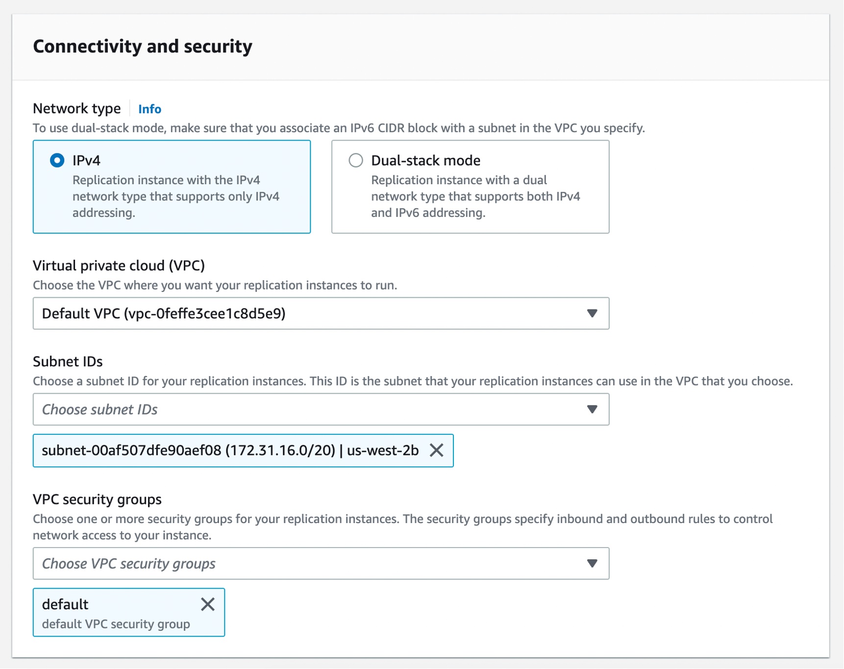
Before you create your migration project, set up an instance profile by choosing Instance profiles in the left pane. An instance profile specifies network and security settings for your DMS Schema Conversion instances. You can create multiple instance profiles and select an instance profile to use for each migration project.
Choose Create instance profile and specify your default VPC or a new VPC, Amazon Simple Storage Service (Amazon S3) bucket to store your schema conversion metadata, and additional settings such as AWS Key Management Service (AWS KMS) keys.
You can create the simplest network configuration with a single VPC configuration. If your source or target data providers are in different VPCs, you can create your instance profile in one of the VPCs, and then link these two VPCs by using VPC peering.
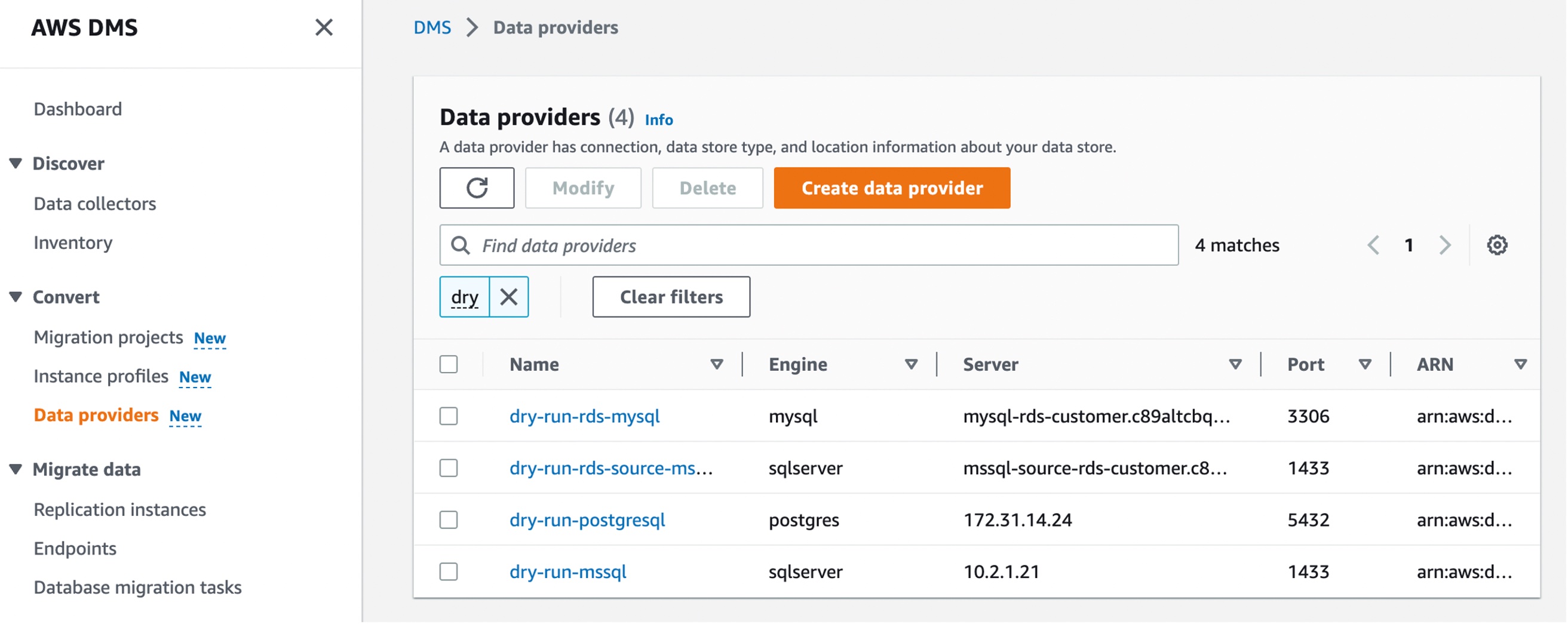
Next, you can add data providers that store the data store type and location information about your source and target databases by choosing Data providers in the left pane. For each database, you can create a single data provider and use it in multiple migration projects.
Your data provider can be a fully managed Amazon RDS instance or a self-managed engine running either on-premises or on an Amazon Elastic Compute Cloud (Amazon EC2) instance.
Choose Create data provider to create a new data provider. You can set the type of the database location manually, such as database engine, domain name or IP address, port number, database name, and so on, for your data provider. Here, I have selected an RDS database instance.
After you create a data provider, make sure that you add database connection credentials in AWS Secrets Manager. DMS Schema Conversion uses this information to connect to a database.
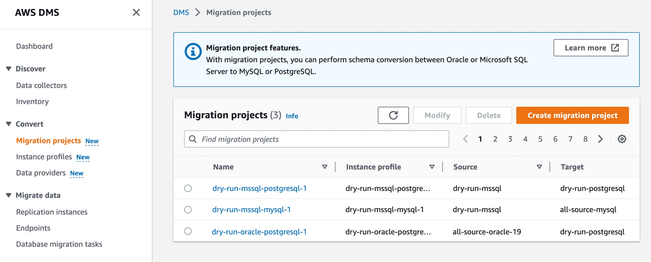
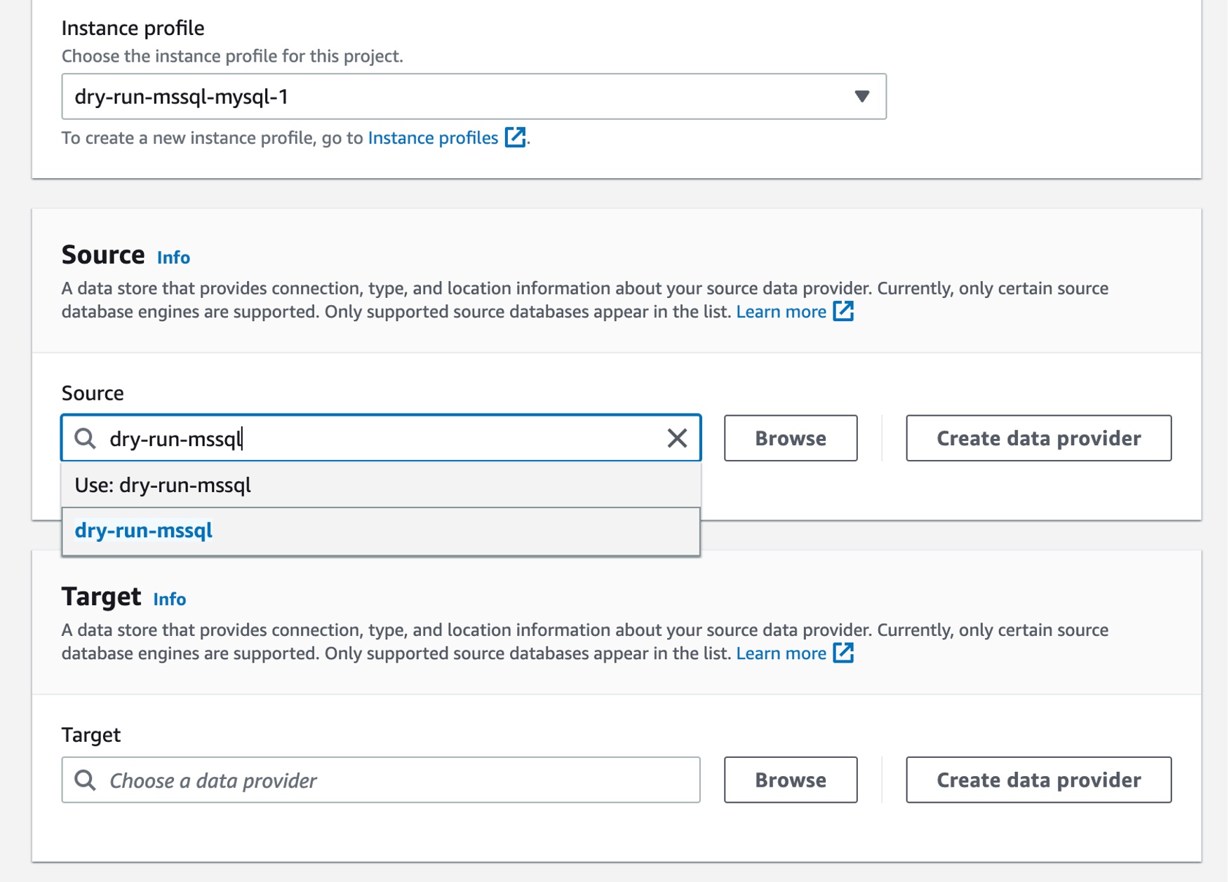
Converting your database schema with AWS DMS Schema Conversion Now, you can create a migration project for DMS Schema Conversion by choosing Migration projects in the left pane. A migration project describes your source and target data providers, your instance profile, and migration rules. You can also create multiple migration projects for different source and target data providers.
Choose Create migration project and select your instance profile and source and target data providers for DMS Schema Conversion.
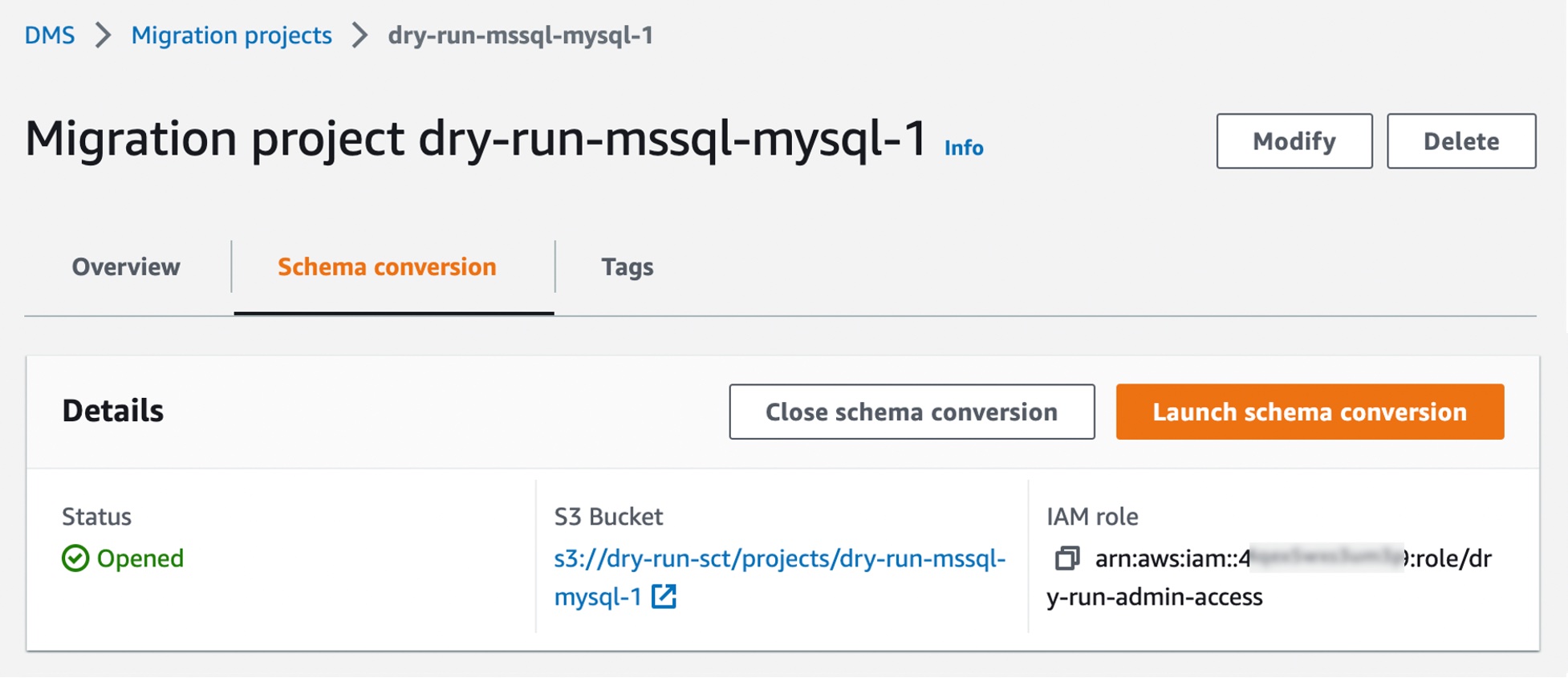
After creating your migration project, you can use the project to create assessment reports and convert your database schema. Choose your migration project from the list, then choose the Schema conversion tab and click Launch schema conversion.
Migration projects in DMS Schema Conversion are always serverless. This means that AWS DMS automatically provisions the cloud resources for your migration projects, so you don’t need to manage schema conversion instances.
Of course, the first launch of DMS Schema Conversion requires starting a schema conversion instance, which can take up to 10–15 minutes. This process also reads the metadata from the source and target databases. After a successful first launch, you can access DMS Schema Conversion faster.
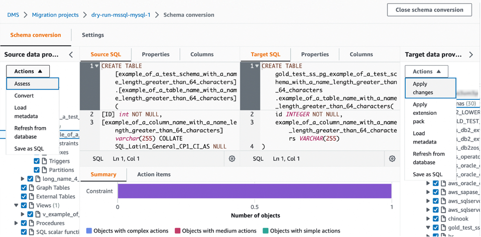
An important part of DMS Schema Conversion is that it generates a database migration assessment report that summarizes all of the schema conversion tasks. It also details the action items for schema that cannot be converted to the DB engine of your target database instance. You can view the report in the AWS DMS console or export it as a comma-separated value (.csv) file.
To create your assessment report, choose the source database schema or schema items that you want to assess. After you select the checkboxes, choose Assess in the Actions menu in the source database pane. This report will be archived with .csv files in your S3 bucket. To change the S3 bucket, edit the schema conversion settings in your instance profile.
Then, you can apply the converted code to your target database or save it as a SQL script. To apply converted code, choose Convert in the pane of Source data provider and then Apply changes in the pane of Target data provider.
Once the schema has been converted successfully, you can move on to the database migration phase using AWS DMS. To learn more, see Getting started with AWS Database Migration Service in the AWS documentation.
Now Available AWS DMS Schema Conversion is now available in the US East (Ohio), US East (N. Virginia), US West (Oregon), Asia Pacific (Singapore), Asia Pacific (Sydney), Asia Pacific (Tokyo), Europe (Frankfurt), Europe (Ireland), and Europe (Stockholm) Regions, and you can start using it today.
With Amazon Redshift, you can analyze data in the cloud at any scale. Amazon Redshift offers native data protection capabilities to protect your data using automatic and manual snapshots. This works great by itself, but when you’re using other AWS services, you have to configure more than one tool to manage your data protection policies.
To make this easier, I am happy to share that we added support for Amazon Redshift in AWS Backup. AWS Backup allows you to define a central backup policy to manage data protection of your applications and can now also protect your Amazon Redshift clusters. In this way, you have a consistent experience when managing data protection across all supported services. If you have a multi-account setup, the centralized policies in AWS Backup let you define your data protection policies across all your accounts within your AWS Organizations. To help you meet your regulatory compliance needs, AWS Backup now includes Amazon Redshift in its auditor-ready reports. You also have the option to use AWS Backup Vault Lock to have immutable backups and prevent malicious or inadvertent changes.
Let’s see how this works in practice.
Using AWS Backup with Amazon Redshift The first step is to turn on the Redshift resource type for AWS Backup. In the AWS Backup console, I choose Settings in the navigation pane and then, in the Service opt-in section, Configure resources. There, I toggle the Redshift resource type on and choose Confirm.
Now, I can create or update a backup plan to include the backup of all, or some, of my Redshift clusters. In the backup plan, I can define how often these backups should be taken and for how long they should be kept. For example, I can have daily backups with one week of retention, weekly backups with one month of retention, and monthly backups with one year of retention.
I can also create on-demand backups. Let’s see this with more details. I choose Protected resources in the navigation pane and then Create on-demand backup.
I select Redshift in the Resource type dropdown. In the Cluster identifier, I select one of my clusters. For this workload, I need two weeks of retention. Then, I choose Create on-demand backup.
My data warehouse is not huge, so after a few minutes, the backup job has completed.
I now see my Redshift cluster in the list of the resources protected by AWS Backup.
In the Protected resources list, I choose the Redshift cluster to see the list of the available recovery points.
When I choose one of the recovery points, I have the option to restore the full data warehouse or just a table into a new Redshift cluster.
I now have the possibility to edit the cluster and database configuration, including security and networking settings. I just update the cluster identifier, otherwise the restore would fail because it must be unique. Then, I choose Restore backup to start the restore job.
After some time, the restore job has completed, and I see the old and the new clusters in the Amazon Redshift console. Using AWS Backup gives me a simple centralized way to manage data protection for Redshift clusters as well as many other resources in my AWS accounts.
There is no additional cost for using AWS Backup compared to the native snapshot capability of Amazon Redshift. Your overall costs depend on the amount of storage and retention you need. For more information, see AWS Backup pricing.
In May 2022, we announced our quest to simplify databases – building them, maintaining them, integrating them. Our goal is to empower you with the tools to run a database that is powerful, scalable, with world-beating performance without any hassle. And we first set our sights on reimagining the database development experience for every type of user – not just database experts.
Over the past couple of months, we’ve been working to create just that, while learning some very important lessons along the way. As it turns out, building a global relational database product on top of Workers pushes the boundaries of the developer platform to their absolute limit, and often beyond them, but in a way that’s absolutely thrilling to us at Cloudflare. It means that while our progress might seem slow from outside, every improvement, bug fix or stress test helps lay down a path for all of our customers to build the world’s most ambitious serverless application.
However, as we continue down the road to making D1 production ready, it wouldn’t be “the Cloudflare way” unless we stopped for feedback first – even though it’s not quite finished yet. In the spirit of Developer Week, there is no better time to introduce the D1 open alpha!
An “open alpha” is a new concept for us. You’ll likely hear the term “open beta” on various announcements at Cloudflare, and while it makes sense for many products here, it wasn’t quite right for D1. There are still some crucial pieces that are still in active development and testing, so before we release the fully-formed D1 as a public beta for you to start building real-world apps with, we want to make sure everybody can start to get a feel for the product on their hobby apps or side-projects.
What’s included in the alpha?
While a lot is still changing behind the scenes with D1, we’ve put a lot of thought into how you, as a developer, interact with it – even if you’re new to databases.
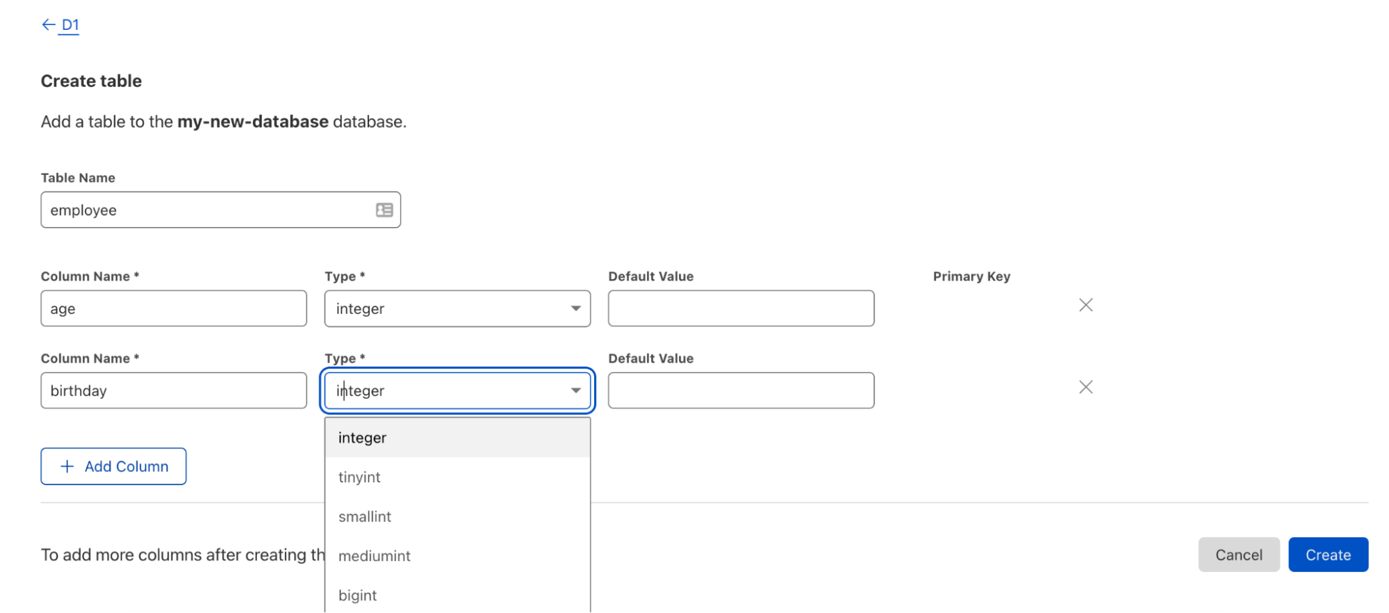
Using the D1 dashboard
In a few clicks you can get your D1 database up and running right from within your dashboard. In our D1 interface, you can create, maintain and view your database as you please. Changes made in the UI are instantly available to your Worker – no redeploy required!
Use Wrangler
If you’re looking to get your hands a little dirty, you can also work with your database using our Wrangler CLI. Create your database and begin adding your data manually or bootstrap your database with one of two ways:
Migrations are a way to version your database changes. With D1, you can create a migration and then apply it to your database.
To create the migration, execute:
wrangler d1 migrations create <my-database-name> <short description of migration>
This will create an SQL file in a migrations folder where you can then go ahead and add your queries. Then apply the migrations to your database by executing:
wrangler d1 migrations apply <my-database-name>
Access D1 from within your Worker
You can attach your D1 to a Worker by adding the D1 binding to your wrangler.toml configuration file. Then interact with D1 by executing queries inside your Worker like so:
export default {
 async fetch(request, env) {
   const { pathname } = new URL(request.url);

   if (pathname === "/api/beverages") {
     const { results } = await env.DB.prepare(
       "SELECT * FROM Customers WHERE CompanyName = ?"
     )
       .bind("Bs Beverages")
       .all();
     return Response.json(results);
   }

   return new Response("Call /api/beverages to see Bs Beverages customers");
 },
};
Or access D1 from within your Pages Function
In this Alpha launch, D1 also supports integration with Cloudflare Pages! You can add a D1 binding inside the Pages dashboard, and write your queries inside a Pages Function to build a full-stack application! Check out the full documentation to get started with Pages and D1.
Community built tooling
During our private alpha period, the excitement behind D1 led to some valuable contributions to the D1 ecosystem and developer experience by members of the community. Here are some of our favorite projects to date:
d1-orm
An Object Relational Mapping (ORM) is a way for you to query and manipulate data by using JavaScript. Created by a Cloudflare Discord Community Champion, the d1-orm seeks to provide a strictly typed experience while using D1:
const users = new Model(
    // table name, primary keys, indexes etc
    tableDefinition,
    // column types, default values, nullable etc
    columnDefinitions
)

// TS helper for typed queries
type User = Infer<type of users>;

// ORM-style query builder
const user = await users.First({
    where: {
        id: 1,
    },
});
This is a zero-dependency query builder that provides a simple standardized interface while keeping the benefits and speed of using raw queries over a traditional ORM. While not intended to provide ORM-like functionality, workers-qb makes it easier to interact with the database from code for direct SQL access:
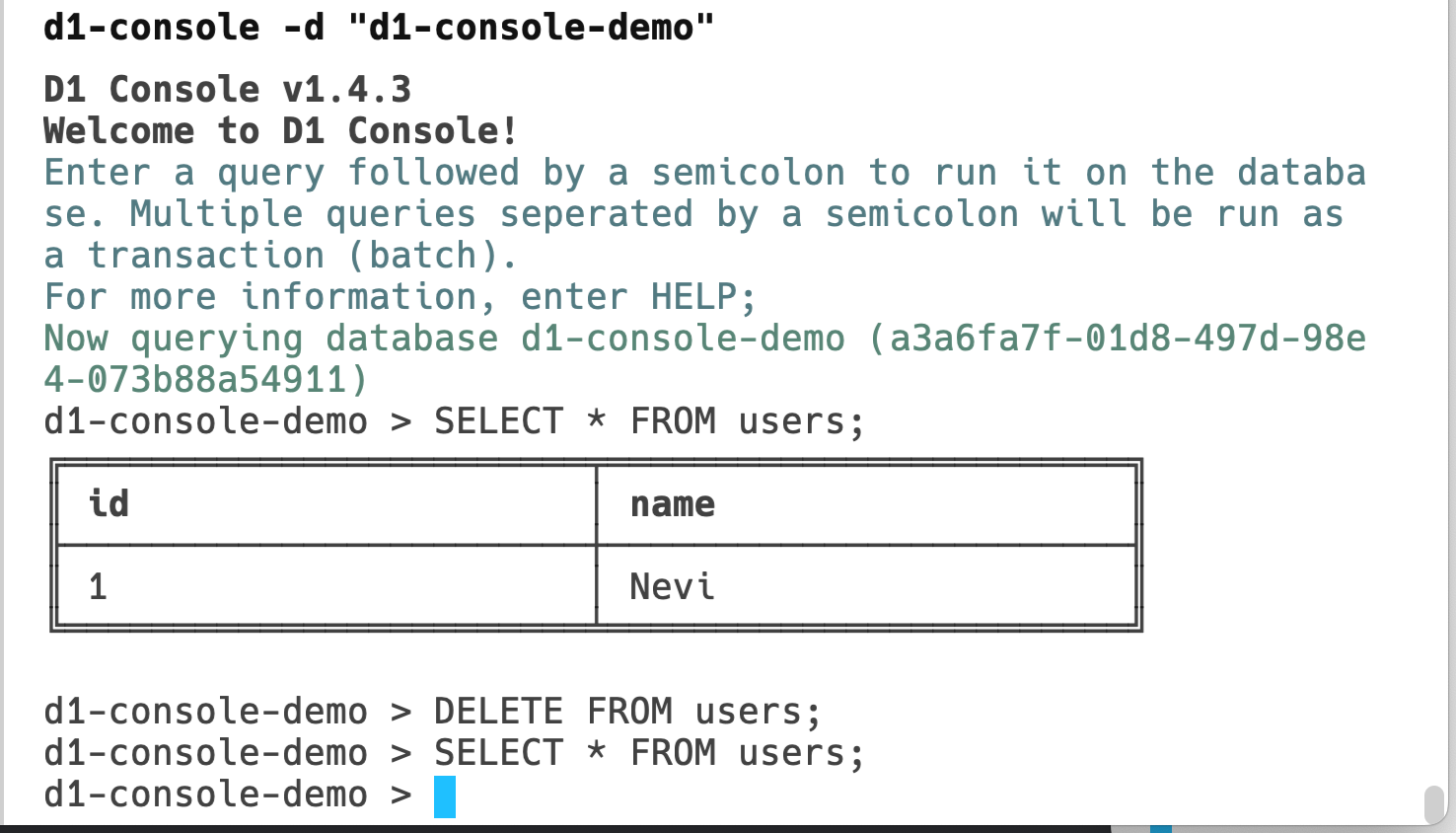
Instead of running the wrangler d1 execute command in your terminal every time you want to interact with your database, you can interact with D1 from within the d1-console. Created by a Discord Community Champion, this gives the benefit of executing multi-line queries, obtaining command history, and viewing a cleanly formatted table output.
While this is a community project today, we plan to natively support a “D1 Console” in the future. For now, get started by checking out the d1-console package here.
Kysely is a type-safe and autocompletion-friendly typescript SQL query builder. With this adapter you can interact with D1 with the familiar Kysely interface:
// Create Kysely instance with kysely-d1
const db = new Kysely<Database>({
  dialect: new D1Dialect({ database: env.DB })
});

// Read row from D1 table
const result = await db
  .selectFrom('kv')
  .selectAll()
  .where('key', '=', key)
  .executeTakeFirst();
The biggest pieces that have been disabled for this alpha release are replication and JavaScript transaction support. While we’ll be rolling out these changes gradually, we want to call out some limitations that exist today that we’re actively working on testing:
Database location: Each D1 database only runs a single instance. It’s created close to where you, as the developer, create the database, and does not currently move regions based on access patterns. Workers running elsewhere in the world will see higher latency as a result.
Concurrency limitations: Under high load, read and write queries may be queued rather than triggering new replicas to be created. As a result, the performance & throughput characteristics of the open alpha won’t be representative of the final product.
Availability limitations: Backups will block access to the DB while they’re running. In most cases this should only be a second or two, and any requests that arrive during the backup will be queued.
You can also check out a more detailed, up-to-date list on D1 alpha Limitations.
Request for feedback
While we can make all sorts of guesses and bets on the kind of databases you want to use D1 for, we are not the users – you are! We want developers from all backgrounds to preview the D1 tech at its early stages, and let us know where we need to improve to make it suitable for your production apps.
For general feedback about your experience and to interact with other folks in the alpha, join our #d1-open-alpha channel in the Cloudflare Developers Discord. We plan to make any important announcements and changes in this channel as well as on our monthly community calls.
To file more specific feature requests (no matter how wacky) and report any bugs, create a thread in the Cloudflare Community forum under the D1 category. We will be maintaining this forum as a way to plan for the months ahead!
Get started
Want to get started right away? Check out our D1 documentation to get started today. Build our classic Northwind Traders demo to explore the D1 experience and deploy your first D1 database!
Amazon Neptune is a fully managed graph database service that makes it easy to build and run applications that work with highly connected datasets. With Neptune, you can use open and popular graph query languages to execute powerful queries that are easy to write and perform well on connected data. You can use Neptune for graph use cases such as recommendation engines, fraud detection, knowledge graphs, drug discovery, and network security.
Neptune has always been fully managed and handles time-consuming tasks such as provisioning, patching, backup, recovery, failure detection and repair. However, managing database capacity for optimal cost and performance requires you to monitor and reconfigure capacity as workload characteristics change. Also, many applications have variable or unpredictable workloads where the volume and complexity of database queries can change significantly. For example, a knowledge graph application for social media may see a sudden spike in queries due to sudden popularity.
Introducing Amazon Neptune Serverless Today, we’re making that easier with the launch of Amazon Neptune Serverless. Neptune Serverless scales automatically as your queries and your workloads change, adjusting capacity in fine-grained increments to provide just the right amount of database resources that your application needs. In this way, you pay only for the capacity you use. You can use Neptune Serverless for development, test, and production workloads and optimize your database costs compared to provisioning for peak capacity.
With Neptune Serverless you can quickly and cost-effectively deploy graphs for your modern applications. You can start with a small graph, and as your workload grows, Neptune Serverless will automatically and seamlessly scale your graph databases to provide the performance you need. You no longer need to manage database capacity and you can now run graph applications without the risk of higher costs from over-provisioning or insufficient capacity from under-provisioning.
With Neptune Serverless, you can continue to use the same query languages (Apache TinkerPop Gremlin, openCypher, and RDF/SPARQL) and features (such as snapshots, streams, high availability, and database cloning) already available in Neptune.
Let’s see how this works in practice.
Creating an Amazon Neptune Serverless Database In the Neptune console, I choose Databases in the navigation pane and then Create database. For Engine type, I select Serverless and enter my-database as the DB cluster identifier.
I can now configure the range of capacity, expressed in Neptune capacity units (NCUs), that Neptune Serverless can use based on my workload. I can now choose a template that will configure some of the next options for me. I choose the Production template that by default creates a read replica in a different Availability Zone. The Development and Testing template would optimize my costs by not having a read replica and giving access to DB instances that provide burstable capacity.
Finally, I choose Create database. After a few minutes, the database is ready to use. In the list of databases, I choose the DB identifier to get the Writer and Reader endpoints that I am going to use later to access the database.
Using Amazon Neptune Serverless There is no difference in the way you use Neptune Serverless compared to a provisioned Neptune database. I can use any of the query languages supported by Neptune. For this walkthrough, I choose to use openCypher, a declarative query language for property graphs originally developed by Neo4j that was open-sourced in 2015 and contributed to the openCypher project.
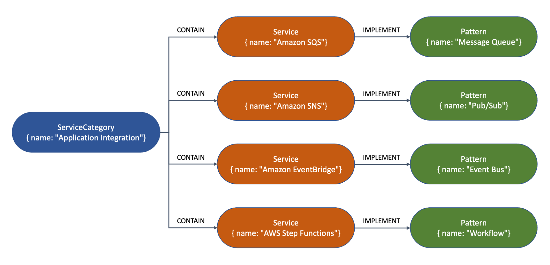
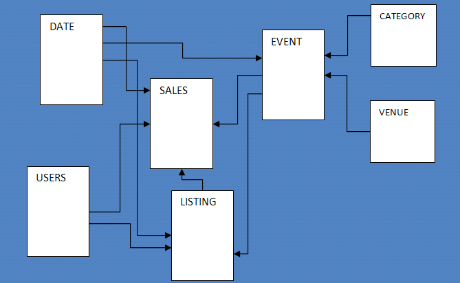
With a property graph I can represent connected data. In this case, I want to create a simple graph that shows how some AWS services are part of a service category and implement common enterprise integration patterns.
I use curl to access the WriteropenCypher HTTPS endpoint and create a few nodes that represent patterns, services, and service categories. The following commands are split into multiple lines in order to improve readability.
This is a visual representation of the nodes and their relationships for the graph created by the previous command. The type (such as Service or Pattern) and properties (such as name) are shown inside each node. The arrows represent the relationships (such as CONTAIN or IMPLEMENT) between the nodes.
Now, I query the database to get some insights. To query the database, I can use either a Writer or a Reader endpoint. First, I want to know the name of the service implementing the “Message Queue” pattern. Note how the syntax of openCypher resembles that of SQL with MATCH instead of SELECT.
There are many options now that I have this graph database up and running. I can add more data (services, categories, patterns) and more relationships between the nodes. I can focus on my application and let Neptune Serverless manage capacity and infrastructure for me.
Availability and Pricing Amazon Neptune Serverless is available today in the following AWS Regions: US East (Ohio, N. Virginia), US West (N. California, Oregon), Asia Pacific (Tokyo), and Europe (Ireland, London).
With Neptune Serverless, you only pay for what you use. The database capacity is adjusted to provide the right amount of resources you need in terms of Neptune capacity units (NCUs). Each NCU is a combination of approximately 2 gibibytes (GiB) of memory with corresponding CPU and networking. The use of NCUs is billed per second. For more information, see the Neptune pricing page.
Having a serverless graph database opens many new possibilities. To learn more, see the Neptune Serverless documentation. Let us know what you build with this new capability!
In this blog post, you will learn how to set up backups for your Zabbix environment. There’s a wide variety of different options when it comes to taking backups of our Zabbix environment, for us, it will just be a matter of choosing the right fit.
Introduction
Monitoring is an important part of our IT infrastructure and often times when our monitoring isn’t working for a certain period, we feel like we are blind as to what is going on with our different IT components. As such, taking backups of our Zabbix environment is an important part of running a production Zabbix environment, as we do want to be prepared for a possible issue that might corrupt or even lose our data. It’s always a possibility and as such we should be prepared.
For Zabbix, there are a few different methods on how to take backups and it all starts at the database level. Both the Zabbix frontend as well as the Zabbix server write their data into the Zabbix database as we can see in the illustration below:
This means that both our configuration as well as all of our collected values are present in the same Zabbix database and if we take a database backup, we back up (almost) everything we need. So, let’s start there and have a look at how we can make a database backup.
How to
MySQL backups
Let’s start with the most used variant of Zabbix databases: MySQL and it’s forks like MariaDB and Percona. All of them can easily be backed up using built-in functionality like the MySQLDump command and we can then use other industry standards to get things going. First, we have to understand the tables in our database though. Most of the tables in your Zabbix environment contain configuration data and as such, they are all important to backup. There are a few tables that we need to consider, however, as they can contain Giga or even Terabytes of data. These are the History, Trends and Events tables:
It is possible to omit these tables from your backup and make smaller, more manageable backups. To make the backup we can then start using tools like MySQLDump:
Once we have taken a backup, we can easily import that back into our environment using the MySQLImport command or simply using the cat command:
Do not forget, taking and importing large backups can take a long time. This completely depends on your MySQL database performance tuning settings as well as the underlying resources like CPU, Memory and Disk I/O. Also, make sure to check out the MySQL documentation:
Alternatively, it’s also possible to create backups using tools like xtrabackup and mariadbbackup.
PostgreSQL backups
We can actually use the same kinds of methods for the PostgreSQL backups. Keep the required tables in mind and fire away with the built-in tools:
Then we can restore it by loading the file into postgres:
What about the configuration files?
Once we have a database backup, everything is backed up, right? Well, almost everything. With just a database backup we are quite safe, but (and this is oftentimes overlooked) there are a lot of configuration files and perhaps even custom scripts we need to take into account! There are three parts to this story – the Zabbix server, the Zabbix frontend, and also the Zabbix additional components. All of them have their own set of configuration files and locations that are used for storing custom scripts.
The Zabbix frontend location and configuration files can be different, depending on the environment, as we have a few choices to make. Are we running Apache or Nginx? On what Linux distribution? All of these have to be considered when making configuration backups. In general, the locations for the configuration would be:
/etc/nginx/
/etc/httpd/
/etc/apache2
There’s also a symlink to the Zabbix frontend configuration file located in /etc/zabbix/ but we will get to that one in a bit.
Then we have the Zabbix server itself, which keeps its configuration in /etc/zabbix/ and if we’re following best practices any script should be placed in /usr/lib/zabbix. So we need:
/etc/zabbix/
/usr/lib/zabbix
Let’s add them to the list and find a method to back up these files. Crontab is a built-in tool that we can use, but there are definitely other (perhaps better) solutions out there. Let’s add the following to cron:
I also added a find command here, which will serve as our roll-over or rotation toll. It will find files older than 180 days and delete them from /mnt/backup/config_files/. Make sure to pick a good (network) folder to store these files as it’s important to keep these safe. Feel free to change the number of days you’d like to store the files for.
What about the additional components like Zabbix proxy, Zabbix Java gateway and Zabbix web service (used for PDF reporting)?. Well, these have configuration files as well. Make sure to run a backup on the devices running these additional components. As for Zabbix proxies – they have the same file locations as Zabbix server:
For Zabbix Java gateway and Zabbix web service, we can omit the /usr/lib/zabbix/ folder.
Don’t forget the import/export files!
In general, database backups are slow to make, but also slow to import back unless we do not include the history/trends in the backup. But even then, restoring an entire database simply because someone made an error on a single template is a hassle. Zabbix ships with the built-in frontend export functionality, allowing us to export (and then import) entire parts of the configuration instantly! We can use these for a number of different parts of the configuration:
Hosts
Templates
Media types
Maps
images
Host groups (API ONLY)
Template groups (API ONLY)
All of these are available through the Zabbix API allowing us to choose whether we do a manual configuration backup from the frontend, as well as providing us with automation options using that API. You could even manage and update your Zabbix configuration from GIT entirely if you write the right scripts for this.
Frontend backups
To run an export from the frontend simply go to one of the supported sections like Configuration | Templates and select the export data format. When selecting multiple entities, keep in mind that they will all be exported to a single file.
We can then make our edits and import files from the frontend as well:
For Templates this will even result in a nice diff pop-up window, detailing all the changes, deletes and additions to the templates:
API backups
For the API things get a little more complicated as we need to select a mode of execution. Of course, it’s possible to do a curl command from the CLI or even use something like Postman:
Request body
The response will then look something like this:
But this feature really starts to shine once we combine it with our own automation scripts. Use it wisely!
High availability
So, what about high availability? Isn’t that some form of a backup?
Well yes and no. High availability is not an “IT backup” in the form of making sure we can recover something that is broken. But it is a backup in the way that if a Zabbix server instance fails, another one takes over for it. HA is somewhat out of scope for this blog post, but it’s still worth mentioning. There are several solutions to set up Zabbix as a full high availability cluster. For MySQL we can use a Primary/Primary setup, for the frontend we can use load balancing techniques like HAProxy and for the Zabbix server, we can use the built-in high availability method. Combine all of these together and you’ll definitely be able to serve your every (production ready!) need.
Conclusion
To conclude, there are many options to start taking backups of our Zabbix environment. It all starts at the database and these backups are definitely vital to keep things safe in case of disaster. When making the backups, do not forget about the configuration files and custom scripts as well as the frontend backup option. Combining all of these solutions will safeguard our environment, but if that isn’t enough – do not forget about industry standards like snapshots. Even further safeguarding our environment on multiple levels.
I hope you enjoyed reading this blog post. If you have any questions or need help configuring anything on your Zabbix setup feel free to contact me and the team at Opensource ICT Solutions. We build a ton of cool integrations like this and much more!
When we announced D1 in May of this year, we knew it would be the start of something new – our first SQL database with Cloudflare Workers. Prior to D1 we’ve announced storage options like KV (key-value store), Durable Objects (single location, strongly consistent data storage) and R2 (blob storage). But the question always remained “How can I store and query relational data without latency concerns and an easy API?”
The long awaited “Cloudflare Database” was the true missing piece to build your application entirely on Cloudflare’s global network, going from a blank canvas in VSCode to a full stack application in seconds. Compatible with the popular SQLite API, D1 empowers developers to build out their databases without getting bogged down by complexity and having to manage every underlying layer.
Since our launch announcement in May and private beta in June, we’ve made great strides in building out our vision of a serverless database. With D1 still in private beta but an open beta on the horizon, we’re excited to show and tell our journey of building D1 and what’s to come.
The D1 Experience
We knew from Cloudflare Workers feedback that using Wrangler as the mechanism to create and deploy applications is loved and preferred by many. That’s why when Wrangler 2.0 was announced this past May alongside D1, we took advantage of the new and improved CLI for every part of the experience from data creation to every update and iteration. Let’s take a quick look on how to get set up in a few easy steps.
Create your database
With the latest version of Wrangler installed, you can create an initialized empty database with a quick
npx wrangler d1 create my_database_name
To get your database up and running! Now it’s time to add your data.
Bootstrap it
It wouldn’t be the “Cloudflare way” if you had to sit through an agonizingly long process to get set up. So we made it easy and painless to bring your existing data from an old database and bootstrap your new D1 database. You can run
and pass through an existing SQLite .sql file of your choice. Your database is now ready for action.
Develop & Test Locally
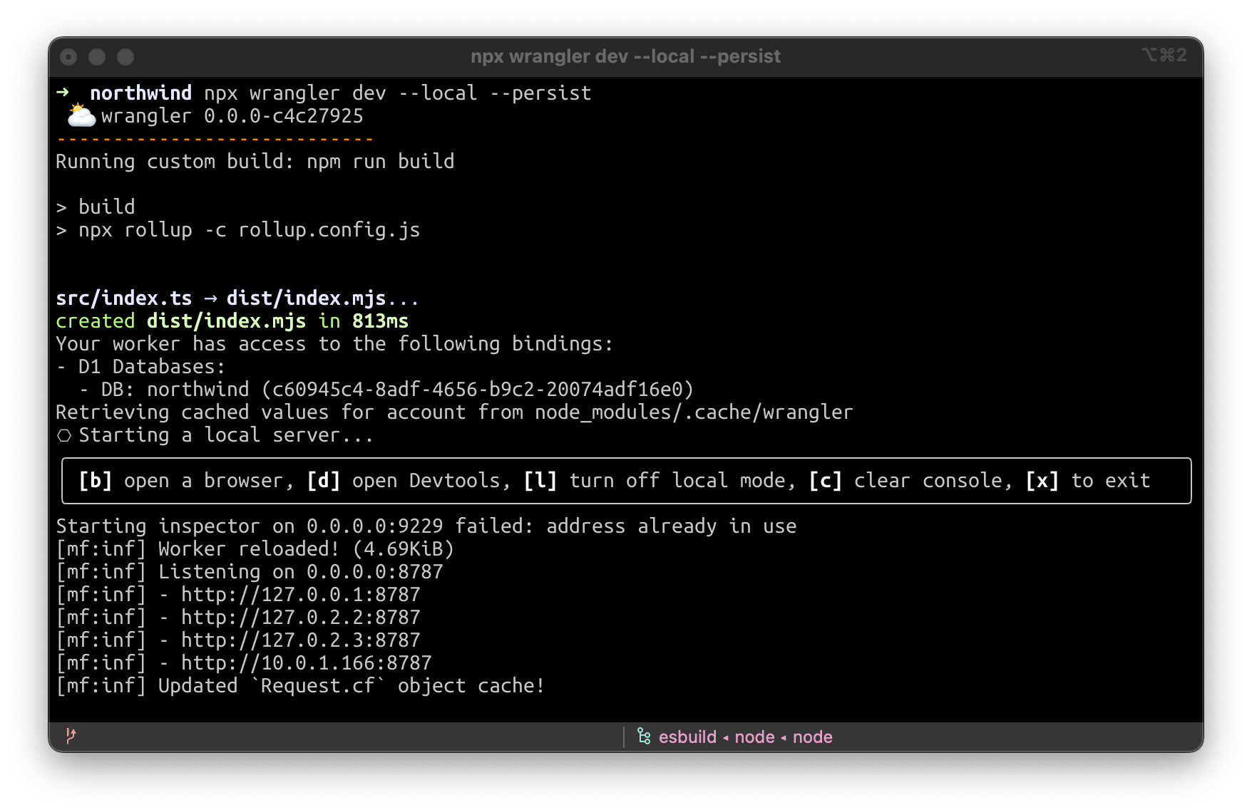
With all the improvements we’ve made to Wrangler since version 2 launched a few months ago, we’re pleased to report that D1 has full remote & local wrangler dev support:
When running wrangler dev -–local -–persist, an SQLite file will be created inside .wrangler/state. You can then use a local GUI program for managing it, like SQLiteFlow (https://www.sqliteflow.com/) or Beekeeper (https://www.beekeeperstudio.io/).
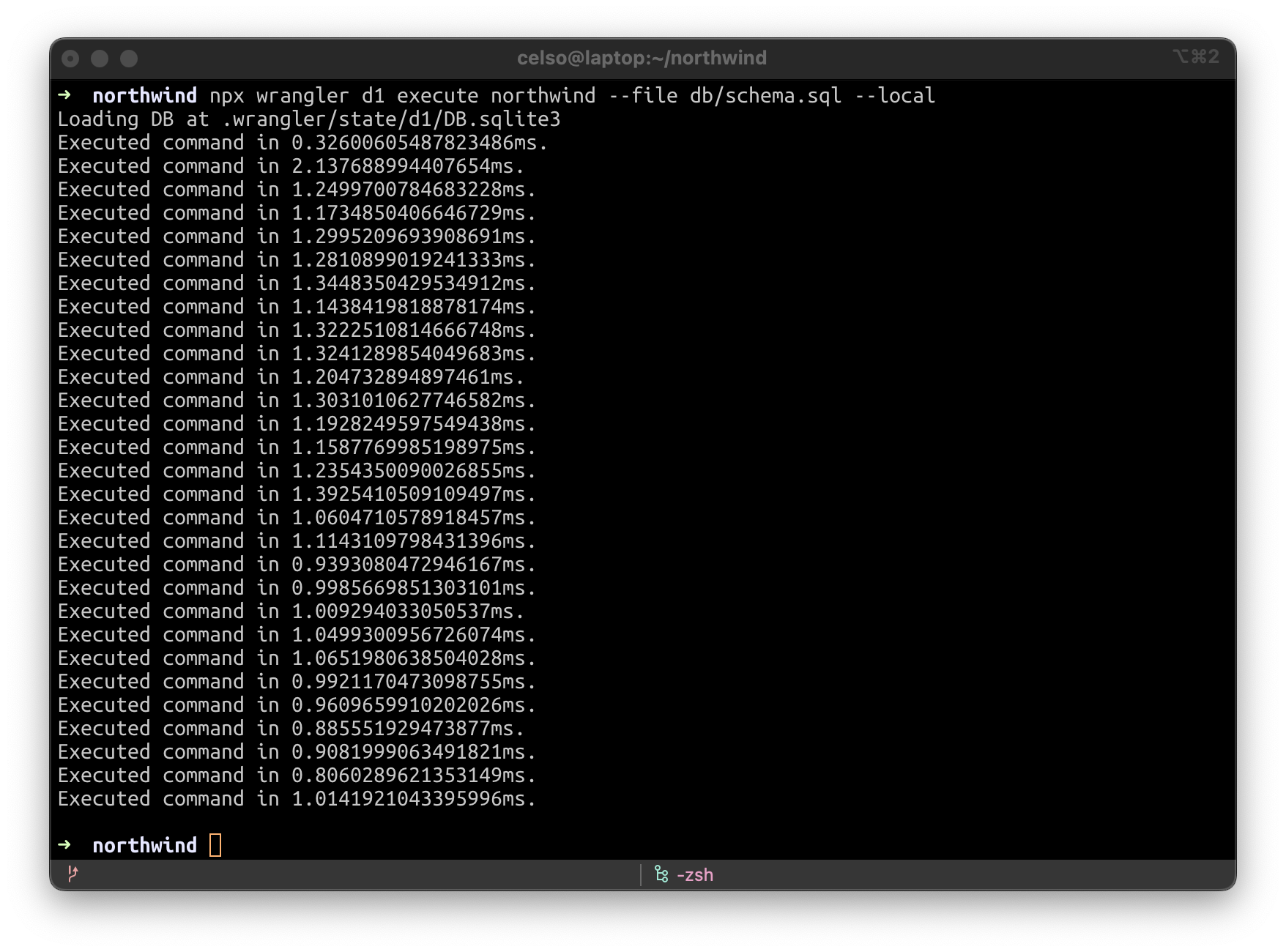
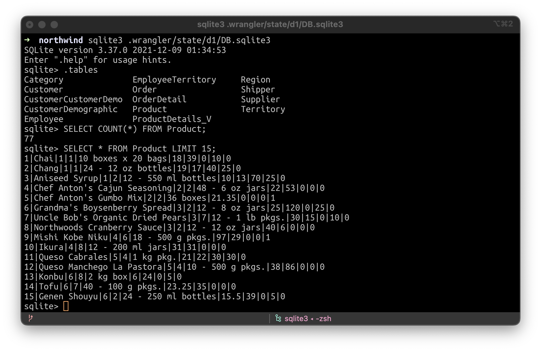
Or you can simply use SQLite directly with the SQLite command line by running sqlite3 .wrangler/state/d1/DB.sqlite3:
Automatic backups & one-click restore
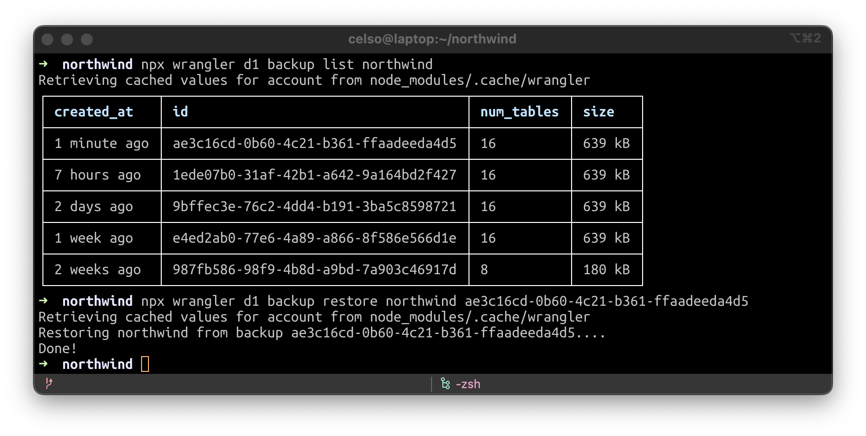
No matter how much you test your changes, sometimes things don’t always go according to plan. But with Wrangler you can create a backup of your data, view your list of backups or restore your database from an existing backup. In fact, during the beta, we’re taking backups of your data every hour automatically and storing them in R2, so you will have the option to rollback if needed.
And the best part – if you want to use a production snapshot for local development or to reproduce a bug, simply copy it into the .wrangler/state directory and wrangler dev –-local –-persist will pick it up!
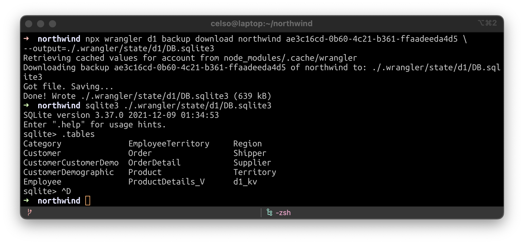
Let’s download a D1 backup to our local disk. It’s SQLite compatible.
Now let’s run our D1 worker locally, from the backup.
Create and Manage from the dashboard
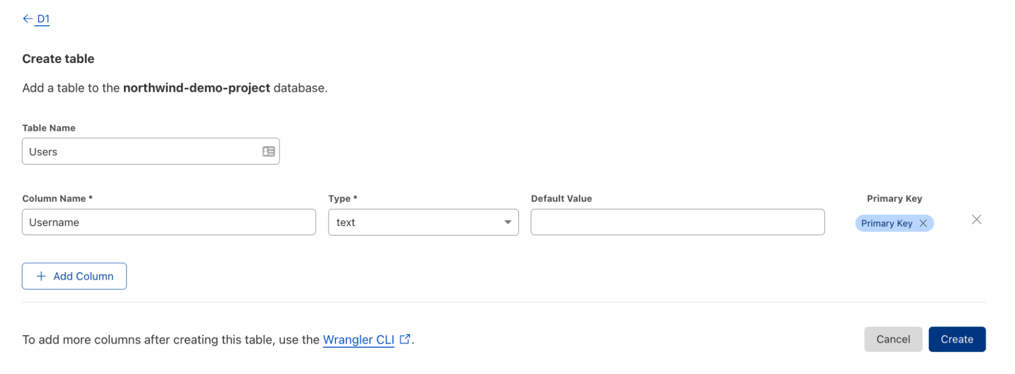
However, we realize that CLIs are not everyone’s jam. In fact, we believe databases should be accessible to every kind of developer – even those without much database experience! D1 is available right from the Cloudflare dashboard giving you near total command parity with Wrangler in just a few clicks. Bootstrapping your database, creating tables, updating your database, viewing tables and triggering backups are all accessible right at your fingertips.
Changes made in the UI are instantly available to your Worker — no deploy required!
We’ve told you about some of the improvements we’ve landed since we first announced D1, but as always, we also wanted to give you a small taste (with some technical details) of what’s ahead. One really important functionality of a database is transactions — something D1 wouldn’t be complete without.
Sneak peek: how we’re bringing JavaScript transactions to D1
With D1, we strive to present a dramatically simplified interface to creating and querying relational data, which for the most part is a good thing. But simplification occasionally introduces drawbacks, where a use-case is no longer easily supported without introducing some new concepts. D1 transactions are one example.
Transactions are a unique challenge
You don’t need to specify where a Cloudflare Worker or a D1 database run—they simply run everywhere they need to. For Workers, that is as close as possible to the users that are hitting your site right this second. For D1 today, we don’t try to run a copy in every location worldwide, but dynamically manage the number and location of read-only replicas based on how many queries your database is getting, and from where. However, for queries that make changes to a database (which we generally call “writes” for short), they all have to travel back to the single Primary D1 instance to do their work, to ensure consistency.
But what if you need to do a series of updates at once? While you can send multiple SQL queries with .batch() (which does in fact use database transactions under the hood), it’s likely that, at some point, you’ll want to interleave database queries & JS code in a single unit of work.
This is exactly what database transactions were invented for, but if you try running BEGIN TRANSACTION in D1 you’ll get an error. Let’s talk about why that is.
Why native transactions don’t work The problem arises from SQL statements and JavaScript code running in dramatically different places—your SQL executes inside your D1 database (primary for writes, nearest replica for reads), but your Worker is running near the user, which might be on the other side of the world. And because D1 is built on SQLite, only one write transaction can be open at once. Meaning that, if we permitted BEGIN TRANSACTION, any one Worker request, anywhere in the world, could effectively block your whole database! This is a quite dangerous thing to allow:
A Worker could start a transaction then crash due to a software bug, without calling ROLLBACK. The primary would be blocked, waiting for more commands from a Worker that would never come (until, probably, some timeout).
Even without bugs or crashes, transactions that require multiple round-trips between JavaScript and SQL could end up blocking your whole system for multiple seconds, dramatically limiting how high an application built with Workers & D1 could scale.
But allowing a developer to define transactions that mix both SQL and JavaScript makes building applications with Workers & D1 so much more flexible and powerful. We need a new solution (or, in our case, a new version of an old solution).
A way forward: stored procedures Stored procedures are snippets of code that are uploaded to the database, to be executed directly next to the data. Which, at first blush, sounds exactly like what we want.
However, in practice, stored procedures in traditional databases are notoriously frustrating to work with, as anyone who’s developed a system making heavy use of them will tell you:
They’re often written in a different language to the rest of your application. They’re usually written in (a specific dialect of) SQL or an embedded language like Tcl/Perl/Python. And while it’s technically possible to write them in JavaScript (using an embedded V8 engine), they run in such a different environment to your application code it still requires significant context-switching to maintain them.
Having both application code and in-database code affects every part of the development lifecycle, from authoring, testing, deployment, rollbacks and debugging. But because stored procedures are usually introduced to solve a specific problem, not as a general purpose application layer, they’re often managed completely manually. You can end up with them being written once, added to the database, then never changed for fear of breaking something.
With D1, we can do better.
The point of a stored procedure was to execute directly next to the data—uploading the code and executing it inside the database was simply a means to that end. But we’re using Workers, a global JavaScript execution platform, can we use them to solve this problem?
It turns out, absolutely! But here we have a few options of exactly how to make it work, and we’re working with our private beta users to find the right API. In this section, I’d like to share with you our current leading proposal, and invite you all to give us your feedback.
When you connect a Worker project to a D1 database, you add the section like the following to your wrangler.toml:
[[ d1_databases ]]
# What binding name to use (e.g. env.DB):
binding = "DB"
# The name of the DB (used for wrangler d1 commands):
database_name = "my-d1-database"
# The D1's ID for deployment:
database_id = "48a4224e-...3b09"
# Which D1 to use for `wrangler dev`:
# (can be the same as the previous line)
preview_database_id = "48a4224e-...3b09"

# NEW: adding "procedures", pointing to a new JS file:
procedures = "./src/db/procedures.js"
That D1 Procedures file would contain the following (note the new db.transaction() API, that is only available within a file like this):
export default class Procedures {
  constructor(db, env, ctx) {
    this.db = db
  }

  // any methods you define here are available on env.DB.Procedures
  // inside your Worker
  async Checkout(cartId: number) {
    // Inside a Procedure, we have a new db.transaction() API
    const result = await this.db.transaction(async (txn) => {

      // Transaction has begun: we know the user can't add anything to
      // their cart while these actions are in progress.
      const [cart, user] = Helpers.loadCartAndUser(cartId)

      // We can update the DB first, knowing that if any of the later steps
      // fail, all these changes will be undone.
      await this.db
        .prepare(`UPDATE cart SET status = ?1 WHERE cart_id = ?2`)
        .bind('purchased', cartId)
        .run()
      const newBalance = user.balance - cart.total_cost
      await this.db
        .prepare(`UPDATE user SET balance = ?1 WHERE user_id = ?2`)
        // Note: the DB may have a CHECK to guarantee 'user.balance' can not
        // be negative. In that case, this statement may fail, an exception
        // will be thrown, and the transaction will be rolled back.
        .bind(newBalance, cart.user_id)
        .run()

      // Once all the DB changes have been applied, attempt the payment:
      const { ok, details } = await PaymentAPI.processPayment(
        user.payment_method_id,
        cart.total_cost
      )
      if (!ok) {
        // If we throw an Exception, the transaction will be rolled back
        // and result.error will be populated:
        // throw new PaymentFailedError(details)

        // Alternatively, we can do both of those steps explicitly
        await txn.rollback()
        // The transaction is rolled back, our DB is now as it was when we
        // started. We can either move on and try something new, or just exit.
        return { error: new PaymentFailedError(details) }
      }

      // This is implicitly called when the .transaction() block finishes,
      // but you can explicitly call it too (potentially committing multiple
      // times in a single db.transaction() block).
      await txn.commit()

      // Anything we return here will be returned by the
      // db.transaction() block
      return {
        amount_charged: cart.total_cost,
        remaining_balance: newBalance,
      }
    })

    if (result.error) {
      // Our db.transaction block returned an error or threw an exception.
    }

    // We're still in the Procedure, but the Transaction is complete and
    // the DB is available for other writes. We can either do more work
    // here (start another transaction?) or return a response to our Worker.
    return result
  }
}
And in your Worker, your DB binding now has a “Procedures” property with your function names available:
const { error, amount_charged, remaining_balance } =
  await env.DB.Procedures.Checkout(params.cartId)

if (error) {
  // Something went wrong, `error` has details
} else {
  // Display `amount_charged` and `remaining_balance` to the user.
}
Multiple Procedures can be triggered at one time, but only one db.transaction() function can be active at once: any other write queries or other transaction blocks will be queued, but all read queries will continue to hit local replicas and run as normal. This API gives you the ability to ensure consistency when it’s essential but with the minimal impact on total overall performance worldwide.
Request for feedback
As with all our products, feedback from our users drives the roadmap and development. While the D1 API is in beta testing today, we’re still seeking feedback on the specifics. However, we’re pleased that it solves both the problems with transactions that are specific to D1 and the problems with stored procedures described earlier:
Code is executing as close as possible to the database, removing network latency while a transaction is open.
Any exceptions or cancellations of a transaction cause an instant rollback—there is no way to accidentally leave one open and block the whole D1 instance.
The code is in the same language as the rest of your Worker code, in the exact same dialect (e.g. same TypeScript config as it’s part of the same build).
It’s deployed seamlessly as part of your Worker. If two Workers bind to the same D1 instance but define different procedures, they’ll only see their own code. If you want to share code between projects or databases, extract a library as you would with any other shared code.
In local development and test, the procedure works just like it does in production, but without the network call, allowing seamless testing and debugging as if it was a local function.
Because procedures and the Worker that define them are treated as a single unit, rolling back to an earlier version never causes a skew between the code in the database and the code in the Worker.
The D1 ecosystem: contributions from the community
We’ve told you about what we’ve been up to and what’s ahead, but one of the unique things about this project is all the contributions from our users. One of our favorite parts of private betas is not only getting feedback and feature requests, but also seeing what ideas and projects come to fruition. While sometimes this means personal projects, with D1, we’re seeing some incredible contributions to the D1 ecosystem. Needless to say, the work on D1 hasn’t just been coming from within the D1 team, but also from the wider community and other developers at Cloudflare. Users have been showing off their D1 additions within our Discord private beta channel and giving others the opportunity to use them as well. We wanted to take a moment to highlight them.
workers-qb
Dealing with raw SQL syntax is powerful (and using the D1 .bind() API, safe against SQL injections) but it can be a little clumsy. On the other hand, most existing query builders assume direct access to the underlying DB, and so aren’t suitable to use with D1. So Cloudflare developer Gabriel Massadas designed a small, zero-dependency query builder called workers-qb:
While you can interact with D1 through both Wrangler and the dashboard, Cloudflare Community champion, Isaac McFadyen created the very first D1 console where you can quickly execute a series of queries right through your terminal. With the D1 console, you don’t need to spend time writing the various Wrangler commands we’ve created – just execute your queries.
This includes all bells and whistles you would expect from a modern database console including multiline input, command history, validation for things D1 may not yet support, and ability to save your Cloudflare credentials for later use.
Check out the full project on GitHub or NPM for more information.
Miniflare test Integration
The Miniflare project, which powers Wrangler’s local development experience, also provides fully-fledged test environments for popular JavaScript test runners, Jest and Vitest. With this comes the concept of Isolated Storage, allowing each test to run independently, so that changes made in one don’t affect the others. Brendan Coll, creator of Miniflare, guided the D1 test implementation to give the same benefits:
import Worker from ‘../src/index.ts’
const { DB } = getMiniflareBindings();

beforeAll(async () => {
  // Your D1 starts completely empty, so first you must create tables
  // or restore from a schema.sql file.
  await DB.exec(`CREATE TABLE entries (id INTEGER PRIMARY KEY, value TEXT)`);
});

// Each describe block & each test gets its own view of the data.
describe(‘with an empty DB’, () => {
  it(‘should report 0 entries’, async () => {
    await Worker.fetch(...)
  })
  it(‘should allow new entries’, async () => {
    await Worker.fetch(...)
  })
])

// Use beforeAll & beforeEach inside describe blocks to set up particular DB states for a set of tests
describe(‘with two entries in the DB’, () => {
  beforeEach(async () => {
    await DB.prepare(`INSERT INTO entries (value) VALUES (?), (?)`)
            .bind(‘aaa’, ‘bbb’)
            .run()
  })
  // Now, all tests will run with a DB with those two values
  it(‘should report 2 entries’, async () => {
    await Worker.fetch(...)
  })
  it(‘should not allow duplicate entries’, async () => {
    await Worker.fetch(...)
  })
])
All the databases for tests are run in-memory, so these are lightning fast. And fast, reliable testing is a big part of building maintainable real-world apps, so we’re thrilled to extend that to D1.
Want access to the private beta?
Feeling inspired?
We love to see what our beta users build or want to build especially when our products are at an early stage. As we march toward an open beta, we’ll be looking specifically for your feedback. We are slowly letting more folks into the beta, but if you haven’t received your “golden ticket” yet with access, sign up here! Once you’ve been invited in, you’ll receive an official welcome email.
In Part I: Compute, Part II: Storage, and Part III: Networking of this series, we introduced strategies to optimize the compute, storage, and networking layers of your AWS architecture for sustainability.
This post, Part IV, focuses on the database layer and proposes recommendations to optimize your databases’ utilization, performance, and queries. These recommendations are based on design principles of AWS Well-Architected Sustainability Pillar.
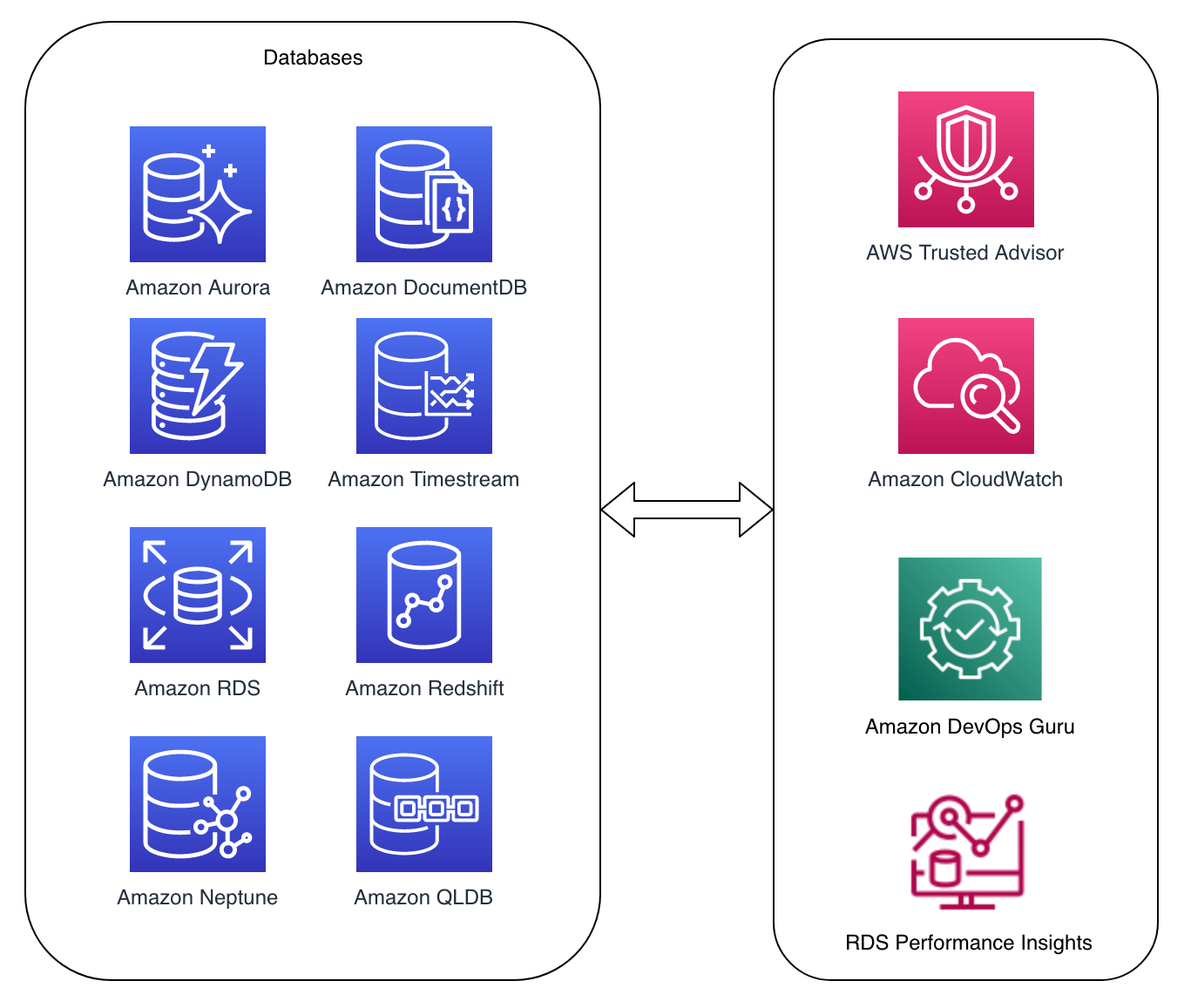
Optimizing the database layer of your AWS infrastructure
Figure 1. AWS database services
As your application serves more customers, the volume of data stored within your databases will increase. Implementing the recommendations in the following sections will help you use databases resources more efficiently and save costs.
Use managed databases
Usually, customers overestimate the capacity they need to absorb peak traffic, wasting resources and money on unused infrastructure. AWS fully managed database services provide continuous monitoring, which allows you to increase and decrease your database capacity as needed. Additionally, most AWS managed databases use a pay-as-you-go model based on the instance size and storage used.
Managed services shift responsibility to AWS for maintaining high average utilization and sustainability optimization of the deployed hardware. Amazon Relational Database Service (Amazon RDS) reduces your individual contribution compared to maintaining your own databases on Amazon Elastic Compute Cloud (Amazon EC2). In a managed database, AWS continuously monitors your clusters to keep your workloads running with self-healing storage and automated scaling.
AWS offers 15+ purpose-built engines to support diverse data models. For example, if an Internet of Things (IoT) application needs to process large amounts of time series data, Amazon Timestream is designed and optimized for this exact use case.
Rightsize, reduce waste, and choose the right hardware
To see metrics, thresholds, and actions you can take to identify underutilized instances and rightsizing opportunities, Optimizing costs in Amazon RDS provides great guidance. The following table provides additional tools and metrics for you to find unused resources:
These tools will help you identify rightsizing opportunities. However, rightsizing databases can affect your SLAs for query times, so consider this before making changes.
We also suggest:
Evaluating if your existing SLAs meet your business needs or if they could be relaxed as an acceptable trade-off to optimize your environment for sustainability.
If any of your RDS instances only need to run during business hours, consider shutting them down outside business hours either manually or with Instance Scheduler.
Consider using a more power-efficient processor like AWS Graviton-based instances for your databases. Graviton2 delivers 2-3.5 times better CPU performance per watt than any other processor in AWS.
Make sure to choose the right RDS instance type for the type of workload you have. For example, burstable performance instances can deal with spikes that exceed the baseline without the need to overprovision capacity. In terms of storage, Amazon RDS provides three storage types that differ in performance characteristics and price, so you can tailor the storage layer of your database according to your needs.
Use serverless databases
Production databases that experience intermittent, unpredictable, or spiky traffic may be underutilized. To improve efficiency and eliminate excess capacity, scale your infrastructure according to its load.
AWS offers relational and non-relational serverless databases that shut off when not in use, quickly restart, and automatically scale database capacity based on your application’s needs. This reduces your environmental impact because capacity management is automatically optimized. By selecting the best purpose-built database for your workload, you’ll benefit from the scalability and fully-managed experience of serverless database services, as shown in the following table.
Amazon Redshift Serverless runs and scales data warehouse capacity; you don’t need to set up and manage data warehouse infrastructure
Amazon Timestream for a time series database service for IoT and operational applications
Amazon Keyspaces for a scalable, highly available, and managed Apache Cassandra–compatible database service
Amazon Quantum Ledger Database for a fully managed ledger database that provides a transparent, immutable, and cryptographically verifiable transaction log owned by a central trusted authority
Use automated database backups and remove redundant data
Manual Amazon RDS backups, unlike automated backups, take a manual snapshot of your database and do not have a retention period set by default. This means that unless you delete a manual snapshot, it will not be removed automatically. Removing manual snapshots you don’t need will use fewer resources, which will reduce your costs. If you want manual snapshots of RDS, you can set an “expiration” with AWS Backup. To keep long-term snapshots of MariaDB, MySQL, and PostgreSQL data, we recommend exporting snapshot data to Amazon Simple Storage Service (Amazon S3). You can also export specific tables or databases. This way, you can move data to “colder” longer-term archival storage instead of keeping it within your database.
Optimize long running queries
Identify and optimize queries that are resource intensive because they can affect the overall performance of your application. By using the Performance Insights dashboard, specifically the Top Dimensions table, which displays the Top SQL, waits, and hosts, you’ll be able to view and download SQL queries to diagnose and investigate further.
You can improve your database performance by monitoring, identifying, and remediating anomalous performance issues. Instead of relying on a database administrator (DBA), AWS offers native tools to continuously monitor and analyze database telemetry, as shown in the following table.
CloudWatch displays instance-level and account-level usage metrics for Amazon RDS. Create CloudWatch alarms to activate and notify you based on metric value thresholds you specify or when anomalous metric behavior is detected. Enable Enhanced Monitoring real-time metrics for the operating system the DB instance runs on.
Amazon RDS Performance Insights collects performance metrics, such as database load, from each RDS DB instance. This data gives you a granular view of the databases’ activity every second. You can enable Performance Insights without causing downtime, reboot, or failover.
Amazon DevOps Guru for RDS uses the data from Performance Insights, Enhanced Monitoring, and CloudWatch to identify operational issues. It uses machine learning to detect and notify of database-related issues, including resource overutilization or misbehavior of certain SQL queries.
Conclusion
In this blog post, we discussed technology choices, design principles, and recommended actions to optimize and increase efficiency of your databases. As your data grows, it is important to scale your database capacity in line with your user load, remove redundant data, optimize database queries, and optimize database performance. Figure 2 shows an overview of the tools you can use to optimize your databases.
Figure 2. Tools you can use on AWS for optimization
In the real world, after a passenger places a GrabFood order from the Grab App, the merchant-partner will prepare the order. A driver-partner will then collect the food and deliver it to the passenger. Have you ever wondered what happens in the backend system? The Grab Order Platform is a distributed system that processes millions of GrabFood or GrabMart orders every day. This post aims to share the journey of how we designed the database solution that powers the order platform.
Background
What are the design goals when building the database solution? We collected the requirements by analysing query patterns and traffic patterns.
Query patterns
Here are some important query examples that the Order Platform supports:
Write queries:
a. Create an order.
b. Update an order.
Read queries:
a. Get order by id.
b. Get ongoing orders by passenger id.
c. Get historical orders by various conditions.
d. Get order statistics (for example, get the number of orders)
We can break down queries into two categories: transactional queries and analytical queries. Transactional queries are critical to online order creation and completion, including the write queries and read queries such as 2a or 2b. Analytical queries like 2c and 2d retrieves historical orders or order statistics on demand. Analytical queries are not essential to the oncall order processing.
Traffic patterns
Grab’s Order Platform processes a significant amount of transaction data every month.
During peak hours, the write Queries per Second (QPS) is three times of primary key reads; whilst the range Queries per Second are four times of the primary key reads.
Design goals
From the query and traffic patterns, we arrived at the following three design goals:
Stability – the database solution must be able to handle high read and write QPS. Online order processing queries must have high availability. Even when some part of the system is down, we must be able to provide a degraded experience to the end users allowing them to still be able to create and complete an order.
Scalability and cost – the database solution must be able to support fast evolution of business requirements, given now we handle up to a million orders per month. The solution must also be cost effective at a large scale.
Consistency – strong consistency for transactional queries, and eventually consistency for analytical queries.
Solution
The first design principle towards a stable and scalable database solution is to use different databases to serve transactional and analytical queries, also known as OLTP and OLAP queries. An OLTP database serves queries critical to online order processing. This table keeps data for only a short period of time. Meanwhile, an OLAP database has the same set of data, but serves our historical and statistical queries. This database keeps data for a longer time.
What are the benefits from this design principle? From a stability point of view, we can choose different databases which can better fulfil our different query patterns and QPS requirements. An OLTP database is the single source of truth for online order processing; any failure in the OLAP database will not affect online transactions. From a scalability and cost point of view, we can choose a flexible database for OLAP to support our fast evolution of business requirements. We can maintain less data in our OLTP database while keeping some older data in our OLAP database.
To ensure that the data in both databases are consistent, we introduced the second design principle – data ingestion pipeline. In Figure 1, Order Platform writes data to the OLTP database to process online orders and asynchronously pushes the data into the data ingestion pipeline. The data ingestion pipeline ensures that the OLAP database data is eventually consistent.
Figure 1: Order Platform database solution overview
Architecture details
OLTP database
There are two categories of OLTP queries, the key-value queries (for example, load by order id) and the batch queries (for example, Get ongoing orders by passenger id). We use DynamoDB as the database to support these OLTP queries.
Why DynamoDB?
Scalable and highly available: the tables of DynamoDB are partitioned and each partition is three-way replicated.
Support for strong consistent reads by primary key.
DynamoDB has a mechanism called adaptive capacity to handle hotkey traffic. Internally, DynamoDB will distribute higher capacity to high-traffic partitions, and isolate frequently accessed items to a dedicated partition. This way, the hotkey can utilise the full capacity of an entire partition, which is up to 3000 read capacity units and 1000 write capacity units.
In each DynamoDB table, it has many items with attributes. In each item, it has a partition key and sort key. The partition key is used for key-value queries, and the sort key is used for range queries. In our case, the table contains multiple order items. The partition key is order ID. We can easily support key-value queries by the partition key.
order_id (PK)
state
pax_id
created_at
pax_id_gsi
order1
Ongoing
Alice
9:00am
order2
Ongoing
Alice
9:30am
order3
Completed
Alice
8:30am
Batch queries like ‘Get ongoing orders by passenger id’ are supported by DynamoDB Global Secondary Index (GSI). A GSI is like a normal DynamoDB table, which also has keys and attributes.
In our case, we have a GSI table where the partition key is the pax_id_gsi. The attribute pax_id_gsi is linked to the main table. It is eventually consistent with the main table that is maintained by DynamoDB. If the Order Platform queries ongoing orders for Alice, two items will be returned from the GSI table.
pax_id_gsi (PK)
created_at (SK)
order_id
Alice
9:00am
order1
Alice
9:30am
order2
We also make use of an advanced feature of GSI named sparse index to support ongoing order queries. When we update order status from ongoing to completed, at the same time, we set the pax_id_gsi to empty, so that the linked item in the GSI will be automatically deleted by DynamoDB. At any time, the GSI table only stores the ongoing orders. We use a sparse index mechanism to control our table size for better performance and to be more cost effective.
The next problem is data retention. This is achieved with the DynamoDB Time To Live (TTL) feature. DynamoDB will auto-scan expired items and delete them. But the challenge is when we add TTL to big tables, it will bring a heavy load to the background scanner and might result in an outage. Our solution is to only add a TTL attribute to the new items in the table. Then, we manually delete the items without TTL attributes, and run a script to delete items with TTL attributes that are too old. After this process, the table size will be quite small, so we can enable the TTL feature on the TTL attribute that we previously added without any concern. The retention period of our DynamoDB data is three months.
Costwise, DynamoDB is charged by storage size and the provision of the read write capability. The provision capability is actually auto scalable. The cost is on-demand. So it’s generally cheaper than RDS.
OLAP database
We use MySQL RDS as the database to support historical and statistical OLAP queries.
Why not Aurora? We choose RDS mainly because it is a mature database solution. Even if Aurora can provide better high-availability, RDS is enough to support our less critical use cases. Costwise, Aurora charges by data storage and the number of requested Input/Output Operations per Second (IOPS). RDS charges only by data storage. As we are using General Purpose (SSD) storage, IOPS is free and supports up to 16k IOPS.
We use MySQL partitioning for data retention. The order table is partitioned by creation time monthly. Since the data access pattern is mostly by month, the partition key can reduce cross-partition queries. Partitions older than six months are dropped at the beginning of each month.
Data ingestion pipeline
Figure 3: Data Ingestion Pipeline Architecture.
A Kafka stream is used to process data in the data ingestion pipeline. We choose the Kafka stream, because it has 99.95% SLA. It is not restricted by the OLTP and OLAP database types.
Even if Kafka can provide 99.95% SLA, there is still the chance of stream producer failures. When the producer fails, we will store the message in an Amazon Simple Queue Service (SQS) and retry. If the retry also fails, it will be moved to the SQS dead letter queue (DLQ), to be consumed at a later time.
On the stream consumer side, we use back-off retry at both stream and database levels to ensure consistency. In a worst-case scenario, we can rewind the stream events from Kafka.
It is important for the data ingestion pipeline to handle duplicate messages and out-of-order messages.
Duplicate messages are handled by the database level unique key (for example, order ID + creation time).
For the out-of-order messages, we implemented the following two mechanisms:
Version update: we only update the most recently updated data. The precision of the update time is in microseconds, which is enough for most of the use cases.
Upsert: if the update events occur before the create events, we simulate an upsert operation.
Impact
After launching our solution this year, we have saved significantly on cloud costs. In the earlier solution, Order Platform synchronously writes to DynamoDB and Aurora and the data is kept forever.
Conclusion
In terms of stability, we use DynamoDB as the critical OLTP database to ensure high availability for online order processing. Scalability wise, we use RDS as the OLAP database to support our quickly evolving business requirements by using a rich, multiple index. Cost efficiency is achieved by data retention in both databases. For consistency, we built a single source of truth OLTP database and an OLAP database that is eventually consistent with the help of the data ingestion pipeline.
What’s next?
Currently, the database solution is running on the production environment. Even though the database solution is proven to be stable, scalable and consistent, we still see some potential areas of improvement.
We use MySQL RDS for OLAP data storage. Even though MySQL is stable and cost effective, it is difficult to serve more complicated queries like free text search. Hence, we plan to explore other NoSQL databases like ElasticSearch.
We hope this post helps you understand how we store Grab orders and fulfil the queries from the Grab Order Platform.
Grab is the leading superapp platform in Southeast Asia, providing everyday services that matter to consumers. More than just a ride-hailing and food delivery app, Grab offers a wide range of on-demand services in the region, including mobility, food, package and grocery delivery services, mobile payments, and financial services across 428 cities in eight countries.
Powered by technology and driven by heart, our mission is to drive Southeast Asia forward by creating economic empowerment for everyone. If this mission speaks to you, join our team today!
With the Graviton Challenge last year, we helped customers migrate to Graviton-based EC2 instances and get up to 40 percent price performance benefit in as little as 4 days. Tens of thousands of customers, including 48 of the top 50 Amazon Elastic Compute Cloud (Amazon EC2) customers, use AWS Graviton processors for their workloads. In addition to EC2, many AWS managed services can run their workloads on Graviton. For most customers, adoption is easy, requiring minimal code changes. However, the effort and time required to move workloads to Graviton depends on a few factors including your software development environment and the technology stack on which your application is built.
This year, we want to take it a step further and make it even easier for customers to adopt Graviton not only through EC2, but also through managed services. Today, we are launching AWS Graviton Fast Start, a new program that makes it even easier to move your workloads to AWS Graviton by providing step-by-step directions for EC2 and other managed services that support the Graviton platform:
Amazon Elastic Compute Cloud (Amazon EC2) – EC2 provides the most flexible environment for a migration and can support many kinds of workloads, such as web apps, custom databases, or analytics. You have full control over the interpreted or compiled code running in the EC2 instance. You can also use many open-source and commercial software products that support the Arm64 architecture.
AWS Lambda – Migrating your serverless functions can be really easy, especially if you use an interpreted runtime such as Node.js or Python. Most of the time, you only have to check the compatibility of your software dependencies. I have shown a few examples in this blog post.
AWS Fargate – Fargate works best if your applications are already running in containers or if you are planning to containerize them. By using multi-architecture container images or images that have Arm64 in their image manifest, you get the serverless benefits of Fargate and the price-performance advantages of Graviton.
Amazon Aurora – Relational databases are at the core of many applications. If you need a database compatible with PostgreSQL or MySQL, you can use Amazon Aurora to have a highly performant and globally available database powered by Graviton.
Amazon Relational Database Service (RDS) – Similarly to Aurora, Amazon RDS engines such as PostgreSQL, MySQL, and MariaDB can provide a fully managed relational database service using Graviton-based instances.
Amazon ElastiCache – When your workload requires ultra-low latency and high throughput, you can speed up your applications with ElastiCache and have a fully managed in-memory cache running on Graviton and compatible with Redis or Memcached.
Amazon EMR – With Amazon EMR, you can run large-scale distributed data processing jobs, interactive SQL queries, and machine learning applications on Graviton using open-source analytics frameworks such as Apache Spark, Apache Hive, and Presto.
Formula 1 racing told us that Graviton2-based C6gn instances provided the best price performance benefits for some of their computational fluid dynamics (CFD) workloads. More recently, they found that Graviton3 C7g instances are 40 percent faster for the same simulations and expect Graviton3-based instances to become the optimal choice to run all of their CFD workloads.
Honeycomb has 100 percent of their production workloads running on Graviton using EC2 and Lambda. They have tested the high-throughput telemetry ingestion workload they use for their observability platform against early preview instances of Graviton3 and have seen a 35 percent performance increase for their workload over Graviton2. They were able to run 30 percent fewer instances of C7g than C6g serving the same workload and with 30 percent reduced latency. With these instances in production, they expect over 50 percent price performance improvement over x86 instances.
Twitter is working on a multi-year project to leverage Graviton-based EC2 instances to deliver Twitter timelines. As part of their ongoing effort to drive further efficiencies, they tested the new Graviton3-based C7g instances. Across a number of benchmarks representative of their workloads, they found Graviton3-based C7g instances deliver 20-80 percent higher performance compared to Graviton2-based C6g instances, while also reducing tail latencies by as much as 35 percent. They are excited to utilize Graviton3-based instances in the future to realize significant price performance benefits.
With all these options, getting the benefits of running all or part of your workload on AWS Graviton can be easier than you expect. To help you get started, there’s also a free trial on the Graviton-based T4g instances for up to 750 hours per month through December 31st, 2022.
Last year at re:Invent, we introduced the preview of Amazon Redshift Serverless, a serverless option of Amazon Redshift that lets you analyze data at any scale without having to manage data warehouse infrastructure. You just need to load and query your data, and you pay only for what you use. This allows more companies to build a modern data strategy, especially for use cases where analytics workloads are not running 24-7 and the data warehouse is not active all the time. It is also applicable to companies where the use of data expands within the organization and users in new departments want to run analytics without having to take ownership of data warehouse infrastructure.
Today, I am happy to share that Amazon Redshift Serverless is generally available and that we added many new capabilities. We are also reducing Amazon Redshift Serverless compute costs compared to the preview.
You can now create multiple serverless endpoints per AWS account and Region using namespaces and workgroups:
A namespace is a collection of database objects and users, such as database name and password, permissions, and encryption configuration. This is where your data is managed and where you can see how much storage is used.
A workgroup is a collection of compute resources, including network and security settings. Each workgroup has a serverless endpoint to which you can connect your applications. When configuring a workgroup, you can set up private or publicly accessible endpoints.
Each namespace can have only one workgroup associated with it. Conversely, each workgroup can be associated with only one namespace. You can have a namespace without any workgroup associated with it, for example, to use it only for sharing data with other namespaces in the same or another AWS account or Region.
In your workgroup configuration, you can now use query monitoring rules to help keep your costs under control. Also, the way Amazon Redshift Serverless automatically scales data warehouse capacity is more intelligent to deliver fast performance for demanding and unpredictable workloads.
Let’s see how this works with a quick demo. Then, I’ll show you what you can do with namespaces and workgroups.
Using Amazon Redshift Serverless In the Amazon Redshift console, I select Redshift serverless in the navigation pane. To get started, I choose Use default settings to configure a namespace and a workgroup with the most common options. For example, I’ll be able to connect using my default VPC and default security group.
With the default settings, the only option left to configure is Permissions. Here, I can specify how Amazon Redshift can interact with other services such as S3, Amazon CloudWatch Logs, Amazon SageMaker, and AWS Glue. To load data later, I give Amazon Redshift access to an S3 bucket. I choose Manage IAM roles and then Create IAM role.
When creating the IAM role, I select the option to give access to specific S3 buckets and pick an S3 bucket in the same AWS Region. Then, I choose Create IAM role as default to complete the creation of the role and to automatically use it as the default role for the namespace.
I choose Save configuration and after a few minutes the database is ready for use. In the Serverless dashboard, I choose Query data to open the Redshift query editor v2. There, I follow the instructions in the Amazon Redshift Database Developer guide to load a sample database. If you want to do a quick test, a few sample databases (including the one I am using here) are already available in the sample_data_dev database. Note also that loading data into Amazon Redshift is not required for running queries. I can use data from an S3 data lake in my queries by creating an external schema and an external table.
The sample database consists of seven tables and tracks sales activity for a fictional “TICKIT” website, where users buy and sell tickets for sporting events, shows, and concerts.
To configure the database schema, I run a few SQL commands to create the users, venue, category, date, event, listing, and sales tables.
Then, I download the tickitdb.zip file that contains the sample data for the database tables. I unzip and load the files to a tickit folder in the same S3 bucket I used when configuring the IAM role.
Now, I can use the COPY command to load the data from the S3 bucket into my database. For example, to load data into the users table:
copy users from 's3://MYBUCKET/tickit/allusers_pipe.txt' iam_role default;
The file containing the data for the sales table uses tab-separated values:
After I load data in all tables, I start running some queries. For example, the following query joins five tables to find the top five sellers for events based in California (note that the sample data is for the year 2008):
select sellerid, username, (firstname ||' '|| lastname) as sellername, venuestate, sum(qtysold)
from sales, date, users, event, venue
where sales.sellerid = users.userid
and sales.dateid = date.dateid
and sales.eventid = event.eventid
and event.venueid = venue.venueid
and year = 2008
and venuestate = 'CA'
group by sellerid, username, sellername, venuestate
order by 5 desc
limit 5;
Now that my database is ready, let’s see what I can do by configuring Amazon Redshift Serverless namespaces and workgroups.
Using and Configuring Namespaces Namespaces are collections of database data and their security configurations. In the navigation pane of the Amazon Redshift console, I choose Namespace configuration. In the list, I choose the default namespace that I just created.
In the Data backup tab, I can create or restore a snapshot or restore data from one of the recovery points that are automatically created every 30 minutes and kept for 24 hours. That can be useful to recover data in case of accidental writes or deletes.
In the Security and encryption tab, I can update permissions and encryption settings, including the AWS Key Management Service (AWS KMS) key used to encrypt and decrypt my resources. In this tab, I can also enable audit logging and export the user, connection, and user activity logs.
In the Datashares tab, I can create a datashare to share data with other namespaces and AWS accounts in the same or different Regions. In this tab, I can also create a database from a share I receive from other namespaces or AWS accounts, and I can see the subscriptions for datashares managed by AWS Data Exchange.
When I create a datashare, I can select which objects to include. For example, here I want to share only the date and event tables because they don’t contain sensitive data.
Using and Configuring Workgroups Workgroups are collections of compute resources and their network and security settings. They provide the serverless endpoint for the namespace they are configured for. In the navigation pane of the Amazon Redshift console, I choose Workgroup configuration. In the list, I choose the default namespace that I just created.
In the Data access tab, I can update the network and security settings (for example, change the VPC, the subnets, or the security group) or make the endpoint publicly accessible. In this tab, I can also enable Enhanced VPC routing to route network traffic between my serverless database and the data repositories I use (for example, the S3 buckets used to load or unload data) through a VPC instead of the internet. To access serverless endpoints that are in another VPC or subnet, I can create a VPC endpoint managed by Amazon Redshift.
In the Limits tab, I can configure the base capacity (expressed in Redshift processing units, or RPUs) used to process my queries. Amazon Redshift Serverless scales the capacity to deal with a higher number of users. Here I also have the option to increase the base capacity to speed up my queries or decrease it to reduce costs.
In this tab, I can also set Usage limits to configure daily, weekly, and monthly thresholds to keep my costs predictable. For example, I configured a daily limit of 200 RPU-hours, and a monthly limit of 2,000 RPU-hours for my compute resources. To control the data-transfer costs for cross-Region datashares, I configured a daily limit of 3 TB and a weekly limit of 10 TB. Finally, to limit the resources used by each query, I use Query limits to time out queries running for more than 60 seconds.
Availability and Pricing Amazon Redshift Serverless is generally available today in the US East (Ohio), US East (N. Virginia), US East (Oregon), Europe (Frankfurt), Europe (Ireland), Europe (London), Europe (Stockholm), and Asia Pacific (Seoul), Asia Pacific (Singapore), Asia Pacific (Sydney), and Asia Pacific (Tokyo) AWS Regions.
With Amazon Redshift Serverless, you pay only for the compute capacity your database consumes when active. The compute capacity scales up or down automatically based on your workload and shuts down during periods of inactivity to save time and costs. Your data is stored in managed storage, and you pay a GB-month rate.
To give you improved price performance and the flexibility to use Amazon Redshift Serverless for an even broader set of use cases, we are lowering the price from $0.5 to $0.375 per RPU-hour for the US East (N. Virginia) Region. Similarly, we are lowering the price in other Regions by an average of 25 percent from the preview price. For more information, see the Amazon Redshift pricing page.
To help you get practice with your own use cases, we are also providing $300 in AWS credits for 90 days to try Amazon Redshift Serverless. These credits are used to cover your costs for compute, storage, and snapshot usage of Amazon Redshift Serverless only.
This blog post was written by Syl Taylor, Professional Services Consultant.
In March 2022, the highly anticipated Go 1.18 was released. Go 1.18 brings to the language some long-awaited features and additions, such as generics. It also brings significant performance improvements for Arm’s 64-bit architecture used in AWS Graviton server processors. In this post, we show how migrating Go workloads from Go 1.17.8 to Go 1.18 can help you run your applications up to 20% faster and more cost-effectively. To achieve this goal, we selected a series of realistic and relatable workloads to showcase how they perform when compiled with Go 1.18.
Overview
Go is an open-source programming language which can be used to create a wide range of applications. It’s developer-friendly and suitable for designing production-grade workloads in areas such as web development, distributed systems, and cloud-native software.
AWS Graviton2 processors are custom-built by AWS using 64-bit Arm Neoverse cores to deliver the best price-performance for your cloud workloads running in Amazon Elastic Compute Cloud (Amazon EC2). They provide up to 40% better price/performance over comparable x86-based instances for a wide variety of workloads and they can run numerous applications, including those written in Go.
Web service throughput
For web applications, the number of HTTP requests that a server can process in a window of time is an important measurement to determine scalability needs and reduce costs.
To demonstrate the performance improvements for a Go-based web service, we selected the popular Caddy web server. To perform the load testing, we selected the hey application, which was also written in Go. We deployed these packages in a client/server scenario on m6g Graviton instances.
The Caddy web server compiled with Go 1.18 brings a 7-8% throughput improvement as compared with the variant compiled with Go 1.17.8.
We conducted a second test where the client downloads a dynamic page on which the request handler performs some additional processing to write the HTTP response content. The performance gains were also noticeable at 10-11%.
Regular expression searches
Searching through large amounts of text is where regular expression patterns excel. They can be used for many use cases, such as:
Checking if a string has a valid format (e.g., email address, domain name, IP address),
Finding all of the occurrences of a string (e.g., date) in a text document,
Identifying a string and replacing it with another.
However, despite their efficiency in search engines, text editors, or log parsers, regular expression evaluation is an expensive operation to run. We recommend identifying optimizations to reduce search time and compute costs.
The following example uses the Go regexp package to compile a pattern and search for the presence of a standard date format in a large generated string. We observed a 13.5% increase in completed executions with a 12% reduction in execution time.
In a second example, we used the Go regexp package to find all of the occurrences of a pattern for character sequences in a string, and then replace them with a single character. We observed a 12% increase in evaluation rate with an 11% reduction in execution time.
As with most workloads, the improvements will vary depending on the input data, the hardware selected, and the software stack installed. Furthermore, with this use case, the regular expression usage will have an impact on the overall performance. Given the importance of regex patterns in modern applications, as well as the scale at which they’re used, we recommend upgrading to Go 1.18 for any software that relies heavily on regular expression operations.
Database storage engines
Many database storage engines use a key-value store design to benefit from simplicity of use, faster speed, and improved horizontal scalability. Two implementations commonly used are B-trees and LSM (log-structured merge) trees. In the age of cloud technology, building distributed applications that leverage a suitable database service is important to make sure that you maximize your business outcomes.
B-trees are seen in many database management systems (DBMS), and they’re used to efficiently perform queries using indexes. When we tested a sample program for inserting and deleting in a large B-tree structure, we observed a 10.5% throughput increase with a 10% reduction in execution time.
On the other hand, LSM trees can achieve high rates of write throughput, thus making them useful for big data or time series events, such as metrics and real-time analytics. They’re used in modern applications due to their ability to handle large write workloads in a time of rapid data growth. The following are examples of databases that use LSM trees:
InfluxDB is a powerful database used for high-speed read and writes on time series data. It’s written in Go and its storage engine uses a variation of LSM called the Time-Structured Merge Tree (TSM).
CockroachDB is a popular distributed SQL database written in Go with its own LSM tree implementation.
Badger is written in Go and is the engine behind Dgraph, a graph database. Its design leverages LSM trees.
When we tested an LSM tree sample program, we observed a 13.5% throughput increase with a 9.5% reduction in execution time.
We also tested InfluxDB using comparison benchmarks to analyze writes and reads to the database server. On the load stress test, we saw a 10% increase of insertion throughput and a 14.5% faster rate when querying at a large scale.
In summary, for databases with an engine written in Go, you’ll likely observe better performance when upgrading to a version that has been compiled with Go 1.18.
Machine learning training
A popular unsupervised machine learning (ML) algorithm is K-Means clustering. It aims to group similar data points into k clusters. We used a dataset of 2D coordinates to train K-Means and obtain the cluster distribution in a deterministic manner. The example program uses an OOP design. We noticed an 18% improvement in execution throughput and a 15% reduction in execution time.
A widely-used and supervised ML algorithm for both classification and regression is Random Forest. It’s composed of numerous individual decision trees, and it uses a voting mechanism to determine which prediction to use. It’s a powerful method for optimizing ML models.
We ran a deterministic example to train a dense Random Forest. The program uses an OOP design and we noted a 20% improvement in execution throughput and a 15% reduction in execution time.
Recursion
An efficient, general-purpose method for sorting data is the merge sort algorithm. It works by repeatedly breaking down the data into parts until it can compare single units to each other. Then, it decides their order in the intermediary steps that will merge repeatedly until the final sorted result. To implement this divide-and-conquer approach, merge sort must use recursion. We ran the program using a large dataset of numbers and observed a 7% improvement in execution throughput and a 4.5% reduction in execution time.
Depth-first search (DFS) is a fundamental recursive algorithm for traversing tree or graph data structures. Many complex applications rely on DFS variants to solve or optimize hard problems in various areas, such as path finding, scheduling, or circuit design. We implemented a standard DFS traversal in a fully-connected graph. Then we observed a 14.5% improvement in execution throughput and a 13% reduction in execution time.
Conclusion
In this post, we’ve shown that a variety of applications, not just those primarily compute-bound, can benefit from the 64-bit Arm CPU performance improvements released in Go 1.18. Programs with an object-oriented design, recursion, or that have many function calls in their implementation will likely benefit more from the new register ABI calling convention.
By using AWS Graviton EC2 instances, you can benefit from up to a 40% price/performance improvement over other instance types. Furthermore, you can save even more with Graviton through the additional performance improvements by simply recompiling your Go applications with Go 1.18.
Performing controlled chaos experiments on your Amazon Relational Database Service (RDS) database instances and validating the application behavior is essential to making sure that your application stack is resilient. How does the application behave when there is a database failover? Will the connection pooling solution or tools being used gracefully connect after a database failover is successful? Will there be a cascading failure if the database node gets rebooted for a few seconds? These are some of the fundamental questions that you should consider when evaluating the resiliency of your database stack. Chaos engineering is a way to effectively answer these questions.
Traditionally, database failure conditions, such as a failover or a node reboot, are often triggered using a script or 3rd party tools. However, at scale, these external dependencies often become a bottleneck and are hard to maintain and manage. Scripts and 3rd party tools can fail when called, whereas a web service is highly available. The scripts and 3rd party tools also tend to require elevated permissions to work, which is a management overhead and insecure from a least privilege access model perspective. This is where AWS Fault Injection Simulator (FIS) comes to the rescue.
AWS Fault Injection Simulator (AWS FIS) is a fully managed service for running fault injection experiments on AWS that makes it easier to improve an application’s performance, observability, and resiliency. Fault injection experiments are used in chaos engineering, which is the practice of stressing an application in testing or production environments by creating disruptive events, such as a sudden increase in CPU or memory consumption, database failover and observing how the system responds, and implementing improvements.
We can define the key phases of chaos engineering as identifying the steady state of the workload, defining a hypothesis, running the experiment, verifying the experiment results and making necessary improvements based on the experiment results. These phases will confirm that you are injecting failures in a controlled environment through well-planned experiments in order to build confidence in the workloads and tools we are using to withstand turbulent conditions.
Example—
Baseline: we have a managed database with a replica and automatic failover enabled.
Hypothesis: failure of a single database instance / replica may slow down a few requests but will not adversely affect our application.
Run experiment: trigger a DB failover.
Verify: confirm/dis-confirm the hypothesis by looking at KPIs for the application (e.g., via CloudWatch metric/alarm).
Methodology and Walkthrough
Let’s look at how you can configure AWS FIS to perform failure conditions for your RDS database instances. For this walkthrough, we’ll look at injecting a cluster failover for Amazon Aurora PostgreSQL. You can leverage an existing Aurora PostgreSQL cluster or you can launch a new cluster by following the steps in the Create an Aurora PostgreSQL DB Cluster documentation.
Step 1: Select the Aurora Cluster.
The Aurora PostgreSQL instance that we’ll use for this walkthrough is provisioned in us-east-1 (N. Virginia), and it’s a cluster with two instances. There is one writer instance and another reader instance (Aurora replica). The cluster is named chaostest, the writer instance is named chaostest-instance-1, and the reader is named chaostest-intance-1-us-east-1a.
The goal is to simulate a failover for this Aurora PostgreSQL cluster so that the existing chaostest-intance-1-us-east-1a reader instance will switch roles and then be promoted as the writer, and the existing chaostest-instance-1 will become the reader.
Step 2: Navigate to the AWS FIS console.
We will now navigate to the AWS FIS console to create an experiment template. Select Create experiment template.
Step 3: Complete the AWS FIS template pre-requisites.
Enter a Description, Name, and select the AWS IAM Role for the experiment template.
The IAM role selected above was pre-created. To use AWS FIS, you must create an IAM role that grants AWS FIS the permissions required so that the service can run experiments on your behalf. The role follows the least privileged model and includes permissions to act on your database clusters like trigger a failover. AWS FIS only uses the permissions that have been delegated explicitly for the role. To learn more about how to create an IAM role with the required permissions for AWS FIS, refer to the FIS documentation.
Step 4: Navigate to the Actions, Target, Stop Condition section of the template.
The next key section of AWS FIS is Action, Target, and Stop Condition.
Action—An action is an activity that AWS FIS performs on an AWS resource during an experiment. AWS FIS provides a set of pre-configured actions based on the AWS resource type. Each Action runs for a specified duration during an experiment, or until you stop the experiment. An action can run sequentially or in parallel.
For our experiment, the Action will be aws:rds:failover-db-cluster.
Target—A target is one or more AWS resources on which AWS FIS performs an action during an experiment. You can choose specific resources or select a group of resources based on specific criteria, such as tags or state.
For our experiment, the target will be the chaostest Aurora PostgreSQL cluster.
Stop Condition—AWS FIS provides the controls and guardrails that you need to run experiments safely on your AWS workloads. A stop condition is a mechanism to stop an experiment if it reaches a threshold that you define as an Amazon CloudWatch alarm. If a stop condition is triggered while the experiment is running, then AWS FIS stops the experiment.
For our experiment, we won’t be defining a stop condition. This is because this simple experiment contains only one action. Stop conditions are especially useful for experiments with a series of actions, to prevent them from continuing if something goes wrong.
Step 5: Configure Action.
Now, let’s configure the Action and Target for our experiment template. Under the Actions section, we will select Add action to get the New action window.
Enter a Name, a Description, and select Action type aws:rds:failover-db-cluster. Start after is an optional setting. This setting allows you to specify an action that should precede the one we are currently configuring.
Step 6: Configure Target.
Note that a Target has been automatically created with the name Clusters-Target-1. Select Save to save the action.
Next, you will edit the Clusters-Target-1 target to select the target, i.e., the Aurora PostgreSQL cluster.
Select Target method as Resource IDs, and select the chaostest cluster. If you are interested to select a group of resources, then select Resource tags, filters and parameters option.
Step 7: Create the experiment template to complete this stage.
We will wrap up the process by selecting the create experiment template.
We will get a warning stating that a stop condition isn’t defined. We’ll enter create in the provided field to create the template.
We will get a success message if the entries are correct and the template will be successfully created.
Step 8: Verify the Aurora Cluster.
Before we run the experiment, let’s double-check the chaostest Aurora Cluster to confirm which instance is the writer and which is the reader.
We confirmed that chaostest-instance-1 is the writer and chaostest-instance-1-us-east-1a is the reader.
Step 9: Run the AWS FIS experiment.
Now we’ll run the FIS experiment. Select Actions, and then select Start for the experiment template.
Select Start experiment and you’ll get another warning to confirm if you really want to start this experiment. Confirm by entering start say Start experiment.
Step 10: Observe the various stages of the experiment.
The experiment will be in initiating, running and will eventually be in completed states.
Step 11: Verify the Aurora Cluster to confirm failover.
Now let’s look at the chaostest Aurora PostgreSQL cluster to check the state. Note that a failover was indeed triggered by FIS and chaostest-instance-1-us-east-1a is the newly promoted writer and chaostest-instance-1 is the reader now.
Step 12: Verify the Aurora Cluster logs.
We can also confirm the failover action by looking at the Logs and events section of the Aurora Cluster.
Clean up
If you created a new Aurora PostgreSQL cluster for this walkthrough, then you can terminate the cluster to optimize the costs by following the steps in the Deleting an Aurora DB cluster documentation.
You can also delete the AWS FIS experiment template by following the steps in the Delete an experiment template documentation.
In this walkthrough, you learned how you can leverage AWS FIS to inject failures into your RDS Instances. To get started with AWS Fault Injection Service for Amazon RDS, refer to the service documentation.
Discovering and solving financial crimes has become a challenge due to an increasing amount of financial data. While storing transactional payment data in a structured table format is useful for searching, filtering, and calculations, it is not always an ideal way to represent transactional data. For example, determining if there is a suspicious financial relationship between entityA and entity B is difficult to visualize in a table. Using tables, we would have to do SQL joins for every possible transaction from entity A to every possible subsequent transaction. We would then have to iterate this process until we found a relationship to entity B. Moreover, certain queries are challenging to run on a relational database management system (RDBMS). For example, it can be quite time consuming to discover which account received a minimum amount of $10,000,000 from other accounts.
Graph databases such as Amazon Neptune can be helpful with performing queries, because they can traverse the data and perform calculations simultaneously. Graphs enable us to represent transactions and parties over a multi-connected network, and discover patterns and chains of connections. It is common to use them in anti-money laundering (AML) applications, as they can help find patterns of suspicious transactions.
We needed a solution that could scale and process millions of transactions, by effectively using high memory and CPU configurations to perform complex queries quickly. As part of our customer demonstration to show how graph databases can help discover financial crimes, we also sourced a large dataset on which to test the solution. We used a graph database, Amazon Elastic Kubernetes Service (EKS), and Amazon Neptune, to search for suspicious financial chains across large amounts of transactional data in minutes.
Overview of our conceptual financial crime discovery solution
Figure 1. Workflow for financial crime discovery
We first needed to find a rules engine that could perform transaction inferencing and reasoning. It had to be able to process various rules on our data, be efficient, and able to scale. Next, we needed a straightforward way to ingest data into the solution. Once we had the data available, we needed to initiate a task to begin our inference job. Finally, we needed a location to store the result for further analysis and persistence, see Figure 1.
Using the AWS Cloud to scale up a graph database
We used multiple AWS services to create a fully automated end-to-end batch-based transaction process, shown in Figure 2. We used RDFox, which is an AWS Marketplace product, created by Oxford Semantic Technologies. RDFox is a high-performance in-memory graph database and semantic reasoner. To orchestrate RDFox, we used Amazon EKS Autoscaler to spin up a cluster to instantiate the RDFox container. Amazon EKS can spin up multiple containers for difference inference jobs and recycle the resources when the job finishes. We also used Amazon Neptune, an Amazon managed distributed graph database that can store up to 64 TiB of the results for diagnosis and long-term retention.
The data is stored in Amazon S3 buckets, which provide a streamlined way to feed a large dataset for processing.
Figure 2. Architecture diagram for financial crime discovery
Financial crimes rules
The power of graphs can help discover financial crimes that are reflected in relationships and monetary transactions. To demonstrate this, we will write two rules to detect two scenarios:
Given two suspicious parties X and Y, find out if there is a transactional relationship between them, and if so, provide the chain that connects them. This is a common scenario that financial institutions must detect.
Given a chain identifying suspicious behavior, find out if the minimum transaction amount that reached the beneficiary exceeds a threshold of Z dollars.
Generating data
To generate data for testing, we used a synthetic data generator written in Python (see GitHub repo in References). The generator built two sets of graph artifacts – parties and transactions. Every transaction is being paired with two random parties, and this iterative process creates a network of connected transactions and parties.
We created a dataset with a small percentage (0.01%) of parties tagged as “Suspicious Party,” to simulate the preceding business scenario. Note that those parties will have transactions going both in and out. In some cases, this will collide with other suspicious parties and establish a chain. This method enables us to get simulated data without engineering the suspicious chains. The test dataset used with this solution comprises 1M transactions and thousands of parties. For more information on generating data, see GitHub: Transaction Chains Data Generator.
Walkthrough of the financial investigator workflow
Once deployed, this solution can assist investigators as follows:
An investigator places the transactions and party data (nt triples) in a subdirectory within the input bucket. Typically, subdirectories can be named as a date or range of dates. In addition, the investigator uploads the particular rules (dlog files) and queries (rq files) that must be processed on the data.
Once the data is ready, the investigator uploads a job spec file (simple JSON, see References section). This contains the description of what resources the job requires (CPUs and memory), along with other configurations for the job.
Once the job spec has been uploaded to the bucket’s subdirectory, the job is automatically initiated. The Kubernetes scheduler will allocate enough resources to initiate the RDFox pod. The containers in the pod will then load, process, query results, and upload them to the output bucket.
Once the data reaches the output bucket, an AWS Lambda function is initiated. This invokes the Amazon Neptune Bulk Loader, which asynchronously loads the results to the Neptune cluster in a parallelized manner.
Once the load completes, the investigator gets an email notification that the job has been completed, and the results are ready for view.
Additionally:
The investigator can upload multiple rules and queries, they will all be processed automatically.
The investigator can launch multiple jobs with different/same data, and with different rules and queries at the same time.
All jobs outputs are saved in a unique job ID subdirectory in the output bucket.
To create the solution in your account, follow the instruction here: GitHub repo
Prerequisites
For this walkthrough, you should have the following prerequisites:
The purpose of this first set of rules is to detect chains that might exist between two suspicious parties. The idea of these chains is to represent all the possible relationships that contain monetary transfers between a suspicious originator and the beneficiary. This will include non-suspicious parties in the chain. The rule tags these chains with the “SuspiciousChain” flag.
This set of rules is designed to tag the chains identified by the first set of rules. It also contains a minimum amount of $100 passed to the beneficiary. We can change the amount to check for different compliance requirements. We tag those chains as “HighValueChain.”
Run the job and check your results
Now we can run our job, with the given data, rules, and two additional queries (to extract “SuspiciousChain” and “HighValueChain” respectively). The result of the queries will be loaded to Amazon Neptune automatically for persistent storage, and is made durably available for further analysis.
Let’s look at the results. The following query can be initiated against RDFox console or Amazon Neptune.
Whoa! Figure 3 might look complicated at first, but this is because we are visualizing every pair of suspicious parties that have a relationship with another suspicious party. Let’s filter the query to look only at a single particular chain, which exceeds a minimum of $100 to the beneficiary. The following query can be executed against RDFox console or Amazon Neptune.
SELECT * WHERE { ?S ?P ?O { SELECT ?S WHERE { ?S a type:HighValueChain .
} Limit 1 } }
Figure 4. Visualizing a particular chain
In Figure 4, we can see that Allison, the suspicious originator of the chain, has sent a transaction to Troy. Troy, who is not suspicious, sent the transaction to Karina. Karina is the suspicious beneficiary. We can also see additional information, such as the transaction amount that Karina received, and the chain length of 2 in this case.
In our testing, we were able to scale up to 500M transactions with 50M parties and process this in less than two hours! And we performed this at a significant lower cost when compared to running constant, fixed similar hardware.
Graph databases are a powerful tool to apply reasoning on complex financial relationships. The combination of Amazon Web Services and the RDFox engine results in an automated, scalable, and cost-effective, thanks to the dynamic Kubernetes Cluster Autoscaler. Customers can use this solution and provide their investigators with a tool they can experiment and reason on financial transactions. This solution simplifies the process, and makes it easier to try different rules and queries on complex large data collections.
Today we are announcing Amazon DynamoDB Standard-Infrequent Access (DynamoDB Standard-IA). A new table class for DynamoDB that reduces storage costs by 60 percent compared to existing DynamoDB Standard tables, and that delivers the same performance, durability, and scaling.
Nowadays, many customers are moving their infrequently accessed data between DynamoDB and Amazon Simple Storage Service (Amazon S3). This means that customers are developing a process to migrate the data and build complex applications that must support two different APIs—one for DynamoDB and another for Amazon S3.
DynamoDB Standard-IA table class is designed for customers who want a cost-optimized solution for storing infrequently accessed data in DynamoDB without changing any application code. Using this new table class, you get the single-digit millisecond read and write performance from DynamoDB and use all of the same APIs.
When you use DynamoDB Standard-IA table class, you will save up to 60 percent in storage costs as compared to using the DynamoDB Standard table class. However, DynamoDB reads and writes for this new table class are priced higher than the Standard tables. Therefore, it is important to understand your use cases before applying this new table class to your tables.
DynamoDB Standard-IA is a great solution if you must store terabytes of data for several years where the data must be highly available, but it is not frequently accessed. An example is social media applications where end users rarely access their old posts. However, these posts remain stored, because if someone scrolls on a profile to see an old photo from 2009, they should be able to retrieve it as fast as if it was a newer post.
E-commerce sites are another good use case. These sites might have a lot of products that are not frequently accessed, but administrators of the site still want to have them available in their store just in case someone wants to buy them. Furthermore, this is a good solution for storing a customer’s previous orders. DynamoDB Standard-IA table offers the ability to retain historical orders at a lower cost.
Get started using DynamoDB Standard-IA Get started using DynamoDB Standard-IA by evaluating the best class for your existing tables.
Go to the table page and select Update the table class in the Actions dropdown to change the table class. Then, choose the new table class and save the changes. You can change the table class for an existing table to be Standard-IA or Standard twice every 30-days with no impact on performance or availability. All of the features of DynamoDB are available when using a table in the Standard-IA table class.
Moreover, you can also create a new table with the DynamoDB Standard-IA table class.
Availability and Pricing DynamoDB Standard-IA is available in all of the AWS Regions, except the China Regions and AWS GovCloud.
For example, DynamoDB Standard-IA storage pricing in US East (N. Virginia) is now $0.10 per GB (60 percent less than DynamoDB Standard), while reads and writes are 25 percent higher.
We’re seeing the use of data analytics expanding among new audiences within organizations, for example with users like developers and line of business analysts who don’t have the expertise or the time to manage a traditional data warehouse. Also, some customers have variable workloads with unpredictable spikes, and it can be very difficult for them to constantly manage capacity.
With Amazon Redshift, you use SQL to analyze structured and semi-structured data across data warehouses, operational databases, and data lakes. Today, I am happy to introduce the public preview of Amazon Redshift Serverless, a new capability that makes it super easy to run analytics in the cloud with high performance at any scale. Just load your data and start querying. There is no need to set up and manage clusters. You pay for the duration in seconds when your data warehouse is in use, for example, while you are querying or loading data. There is no charge when your data warehouse is idle.
Amazon Redshift Serverless automatically provisions the right compute resources for you to get started. As your demand evolves with more concurrent users and new workloads, your data warehouse scales seamlessly and automatically to adapt to the changes. You can optionally specify the base data warehouse size to have additional control on cost and application-specific SLAs.
Amazon Redshift Serverless is ideal when it is difficult to predict compute needs such as variable workloads, periodic workloads with idle time, and steady-state workloads with spikes. This approach is also a good fit for ad-hoc analytics needs that need to get started quickly and for test and development environments.
Let’s see how this works in practice.
Using Amazon Redshift Serverless I go to the Amazon Redshift console and choose the new serverless option. The first time, I set up the serverless endpoint and configure networking and security.
I confirm the default settings that use all subnets in my defaultAmazon Virtual Private Cloud (VPC) and its default security group. Data is always encrypted, and I use the default AWS-owned key. Optionally, I can customize all settings. I can associate now or later the AWS Identity and Access Management (IAM) roles to give permissions to access other AWS resources, for example, to be able to load data from an S3 bucket. The configuration of the serverless endpoint will be shared by all my serverless data warehouses in the same AWS account and Region.
For a quick test, I use the tickit sample dataset so I don’t need to load any data. I prepare a query to get the list of tickets sold per date, sorted to see the dates with more sales first:
SELECT caldate, sum(qtysold) as sumsold
FROM   tickit.sales, tickit.date
WHERE  sales.dateid = date.dateid
GROUP BY caldate
ORDER BY sumsold DESC;
By using the web-based query editor, I don’t need to configure a SQL client or set up the network permissions to reach the serverless endpoint. Instead, I just write my SQL query and run it.
I am a visual person. I enable the Chart option on the right of the result table and select a bar chart.
Satisfied with the clarity of the chart, I export it as an image file. In this way, I can quickly share it or include it in a report.
Amazon Redshift Serverless supports all rich SQL functionality of Amazon Redshift such as semi-structured data support. I can use any JDBC/ODBC-compliant tool or the Amazon Redshift Data API to query my data. To migrate data, I can take a snapshot of an Amazon Redshift provisioned cluster and restore it as serverless. Then, I just need to update my SQL applications to use the new serverless endpoint.
Availability and Pricing Amazon Redshift Serverless is available in public preview in the following AWS Regions: US East (N. Virginia), US West (N. California, Oregon), Europe (Frankfurt, Ireland), Asia Pacific (Tokyo).
With Amazon Redshift Serverless, you pay separately for the compute and storage you use. Compute capacity is measured in Redshift Processing Units (RPUs), and you pay for the workloads in RPU-hours with per-second billing. For storage, you pay for data stored in Amazon Redshift-managed storage and storage used for snapshots, similar to what you’d pay with a provisioned cluster using RA3 instances.
To control your costs, you can specify usage limits and define actions that Amazon Redshift automatically takes if those limits are reached. You can specify usage limits in RPU-hours and associated with a daily, weekly, or monthly duration. Setting higher usage limits can improve the overall throughput of the system, especially for workloads that need to handle high concurrency while maintaining consistently high performance.
Compute resources automatically shutdown behind the scenes when there is no activity and resume when you are loading data, or there are queries coming in. When accessing your S3 data lake via the new serverless endpoint, you do not pay for Amazon Redshift Spectrum separately. You have a unified serverless experience and pay for data lake queries also in RPU-seconds. For more information, see the Amazon Redshift pricing page.
The serverless end point is configured at the AWS account level. If you have multiple teams or projects and want to manage costs separately, you can use separate AWS accounts. You can share data between your provisioned clusters and serverless endpoint and between serverless endpoints across accounts.
To help you get practice, we provide you upfront with $500 in AWS credits to try the Amazon Redshift Serverless public preview. You get the credits when you first create a database with Amazon Redshift Serverless. These credits are used to cover your costs for compute, storage, and snapshot usage of Amazon Redshift Serverless only.
To provide the best experiences, we use technologies like cookies to store and/or access device information. Consenting to these technologies will allow us to process data such as browsing behavior or unique IDs on this site. Not consenting or withdrawing consent, may adversely affect certain features and functions.
Functional
Always active
The technical storage or access is strictly necessary for the legitimate purpose of enabling the use of a specific service explicitly requested by the subscriber or user, or for the sole purpose of carrying out the transmission of a communication over an electronic communications network.
Preferences
The technical storage or access is necessary for the legitimate purpose of storing preferences that are not requested by the subscriber or user.
Statistics
The technical storage or access that is used exclusively for statistical purposes.The technical storage or access that is used exclusively for anonymous statistical purposes. Without a subpoena, voluntary compliance on the part of your Internet Service Provider, or additional records from a third party, information stored or retrieved for this purpose alone cannot usually be used to identify you.
Marketing
The technical storage or access is required to create user profiles to send advertising, or to track the user on a website or across several websites for similar marketing purposes.

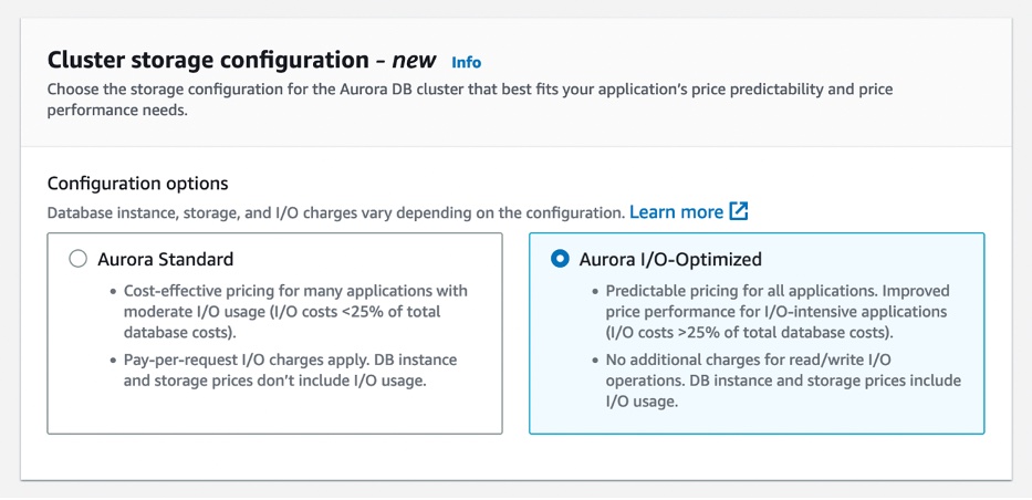
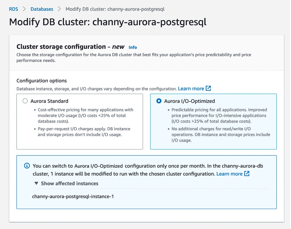

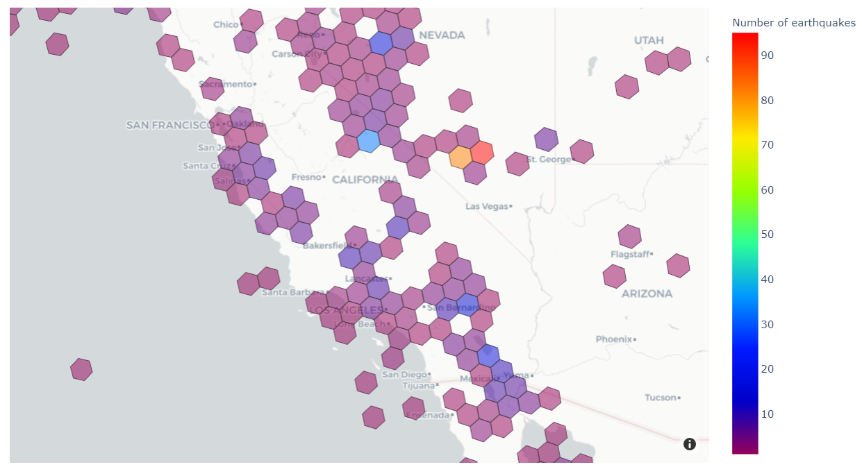


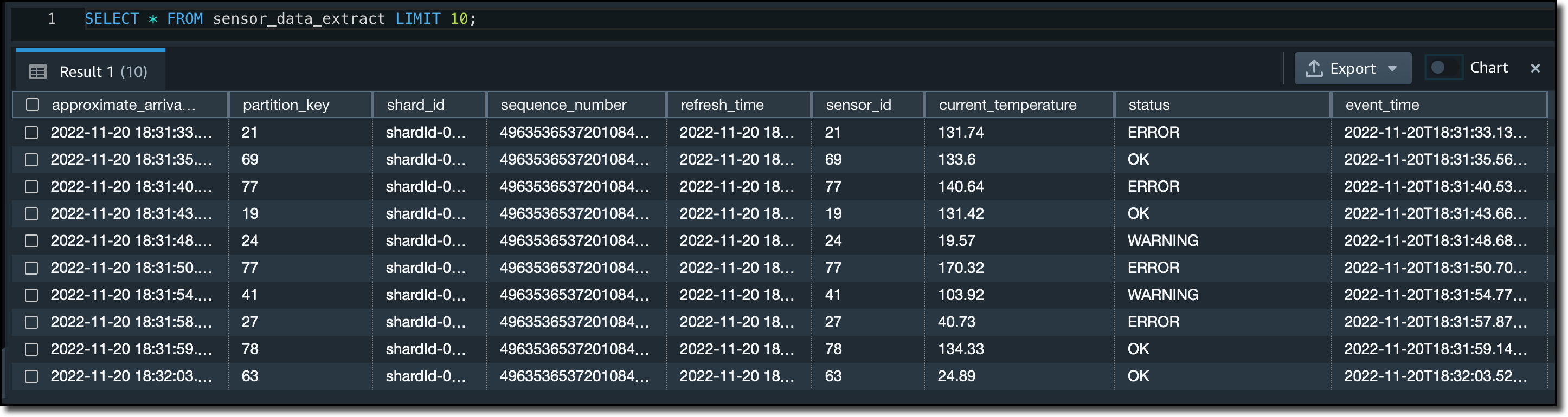
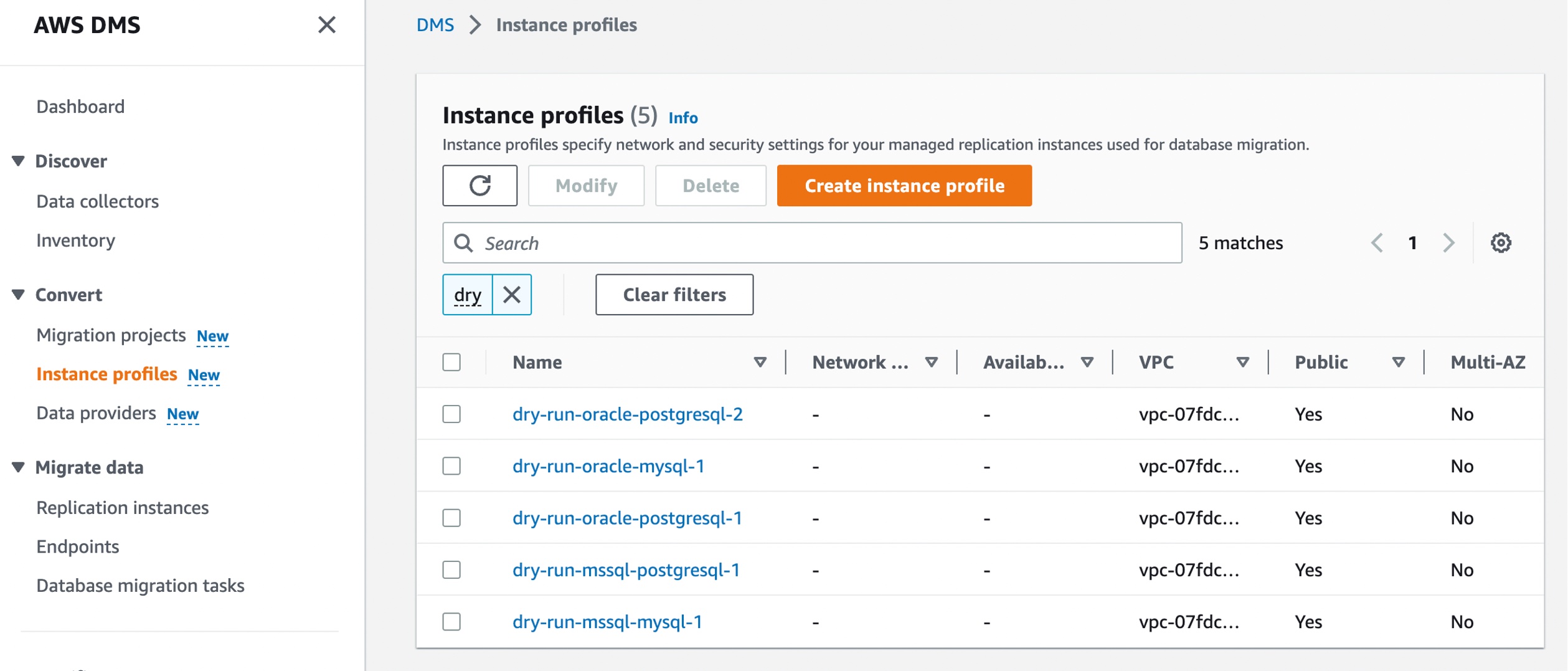 Choose Create instance profile and specify your default VPC or a new VPC,