Tag Archives: Amazon Simple Storage Service (S3)

Introducing an enhanced local IDE experience for AWS Lambda developers

2024-10-31 Julian Wood

Post Syndicated from Julian Wood original https://aws.amazon.com/blogs/compute/introducing-an-enhanced-local-ide-experience-for-aws-lambda-developers/

AWS Lambda is introducing an enhanced local IDE experience to simplify Lambda-based application development. The new features help developers to author, build, debug, test, and deploy Lambda applications more efficiently in their local IDE when using Visual Studio Code (VS Code).

Overview

The IDE experience is part of the AWS Toolkit for Visual Studio Code. A new guided walkthrough helps developers set up their local environment and install required tools. The toolkit includes a set of sample applications which show you how to iterate on your code locally and in the cloud. You can configure and save build settings to speed up application builds. Generate a configuration file to set up the debugging environment for VS Code to attach and launch the step-through debugger. Iterate faster by choosing to sync local application changes quickly to the cloud or perform a full application deploy. Test functions locally and in the cloud and create and share test events to speed up local and cloud testing. There are quick action buttons for build, deploy to cloud, and local or remote invoke. The toolkit integrates with AWS Infrastructure Composer, providing a visual application building experience directly from the IDE.

Using the new features

Installing the extension

To use the updated IDE experience, ensure you have the AWS Toolkit minimum version 3.31.0 installed as a VS Code Extension.

The AWS Toolkit now includes an additional section called Application Builder within the AWS extension side-bar. This allows you to view template resources and create, build, debug, and test serverless applications.

Using Application Builder for existing applications

You can open an existing local application template using Open Folder.

Lambda’s enhanced in-console editing experience allows you to download existing function code and an AWS Serverless Application Model (AWS SAM) template. This allows you to start in the console and more easily move to using infrastructure as code, which is a serverless best practice.

Using the guided walkthrough

The guided walkthrough helps you install dependencies, select an application template, and explains how to use Application Builder to iterate locally and deploy to the cloud.

Choose Open Walkthrough which opens the walkthrough.
Complete installation takes you through a wizard to install required dependencies and select application templates.

The wizard provides download links to install the three dependencies:

If you have installed the dependencies, selecting the links recognizes the installations.

Select Choose your application template, which allows you to create example applications in VS Code.

The Iterate locally tile provides guidance on how to use Application Builder to build and invoke the function, and how to view the results.

Deploy to the cloud provides a link to Configure credentials and explains how to deploy your function to the cloud, remote invoke from your IDE, and view the results.

Creating an application from the samples

The following steps show how to create a function locally from an included template. You build the code artifact, locally test and debug, deploy, and remotely invoke and view results and logs, all without leaving your IDE.

Navigate back to Choose your application template.
New template with visual builder allows you to use Infrastructure Composer to create a new application using a visual canvas.
See more application examples provides additional sample applications across a number of managed runtimes.

There are also two specific example applications to explore Lambda functionality.

Rest API: Learn how to build a synchronous Lambda function behind an API.
File processing.: Learn how to build an asynchronous Amazon S3 file processing application.

Building a synchronous Rest API application

Select Rest API and chose Initialize your project.
Select a language runtime. Select Python for this example.
Open the file explorer, create a folder to download the example application and choose Create Project.

Application Builder downloads the application. This includes the function code hello_world\app.py, with dependencies in requirements.txt, an AWS SAM template, template.yaml file, and an example event trigger, event.json. A README.md file explains the application structure and provides build and deploy instructions.

The Application Builder section populates with the template resources.

The icons provide shortcuts to view, build, and deploy the application.

You can also use the Command Pallete to initiate the AWS SAM commands.

Selecting the Open Template File icon opens the AWS SAM template in Infrastructure Composer.

View the application resources and select Details to edit the template using the visual canvas.

Navigate to the function resource and select Open Function Handler to show the function code.

Building the application

The build step helps you build artifacts from the files in your application project directory.

Select the Build SAM template icon.
Specify build flags allows you to configure AWS SAM builds settings.

Select build settings particular to your configuration. Cached and parallel are useful to speed up future builds. Use container builds your function in a Lambda-like container. This allows you to build applications without having the language runtime and build tools installed locally.

Save parameters adds the default build options in samconfig.toml.

version = 0.1
[default.build.parameters]
template_file = "c:\\Code\\lambda-dx\\Rest-API\\template.yaml"
cached = true
parallel = true
use_container = true

AWS SAM builds the application. It downloads the build container image, installs the dependencies, and copies the function code.

Press any key to close the additional terminal.

Iterate locally: invoke and debug

You can locally invoke and debug your serverless application before uploading it to the cloud. This helps you to test the logic of your function faster. Step-through debugging allows you to identify and fix issues in your application one instruction at a time in your local environment.

Local invoke

In the Application Builder section, navigate to the function and select Local Invoke and Debug Configuration.

Initiating Local Invoke and Debug Configuration

This brings up another window which allows you to configure how to invoke the function locally and set up a debug configuration.

Viewing Local Invoke and Debug Configuration Options

You can create sample event payloads to test your function. Select an event provides a list of common trigger event payloads you can use and customize.

Selecting an example event template

This example application has an included sample event.

Select Local file and choose the events\event.json file.
Select the Invoke button.

This builds the application and locally invokes the function within a Lambda emulation environment, using the event input file.

View the function output within the IDE Output pane.

Viewing function output

Local debugging

You can also debug the function locally using VS Code’s built-in debugger.

Add a breakpoint to the function code.

Adding a breakpoint to the function code

Select the Invoke button again.

This locally invokes the function and attaches a debugger to the Lambda emulation environment.

The debugger stops at the breakpoint and you can view the function variables and call stack.

Viewing step through debugging

Use the VS Code debugger icons to step through the code.

Using VS Code debugger icons to step through the code.

In the Local Invoke and Debug Configuration panel. Chose Save Debug Config.
Choose Add Local Invoke and Debug Configuration.

Saving debug configuration

Enter a debug configuration name which creates a launch.json file and adds the debug configuration.

Naming debug configuration

You can create and save multiple debug configurations for different scenarios. See the AWS SAM documentation for more launch.json configuration options.

Once you save the debug configuration, you can use VS Code’s Run and Debug panel and select which debug configuration to run.

Using the Run and Debug panel

Deploying the application

Navigate to the Application Builder section and chose the Deploy SAM Application icon.

Selecting Deploy SAM Application icon

AWS SAM provides two deployment options:

Sync uses AWS SAM sync to perform an initial CloudFormation deploy and then allows for quick syncing of your application code, which allows for rapid prototyping. Use this for development environments only, as it doesn’t do a full CloudFormation deploy on code changes.
Deploy does a full CloudFormation deploy, which is preferred for non-quick development environments.

Viewing AWS SAM deployment options

Select Sync.
Select Specify required parameters and save as defaults.

Specifying SAM sync parameters

Select a Region to deploy the stack and enter a stack name. It is good practice to specify that this is a dev stack to avoid confusion when using the Deploy option.

Entering dev stack name

Select an existing S3 bucket to store the artifacts, or create a new one.

Selecting S3 bucket

Specify the Sync parameters. Ensure you select Watch as this automatically watches for code changes and quickly syncs code changes to the Lambda service

Setting sync parameters

AWS SAM sync does an initial CloudFormation deploy to build the resources and then waits for code changes.
Make a change to the handler file code and save the file,

Amending code

This performs a quick sync which reduces the time to test in the cloud.

Quickly syncing code

You can use the Deploy option to deploy a non-quick sync test version, amending the stack name to differentiate it from the dev stack.

Naming test version stack

Remote invoke

You can invoke the function in the cloud from your IDE. This allows you to test functionality without having to mock security, external services, or other environment variables.

Once the application is deployed, Application Builder detects changes to samconfig.toml and template.yaml, it updates the resources list with the cloud resources.

Viewing cloud resources

You can browse directly to the CloudFormation stack to view resources.

Browsing to CloudFormation stack

Selecting the function provides quick link functionality, which includes function details and a link directly to the Lambda console for the function.

Viewing function quick link options

Select Invoke in cloud.
Select the same local event file for the local invoke.

Selecting local file for remote invoke

Choose Remote Invoke.

The function invokes in the cloud using the local test event and displays the remote invoke results in the local IDE Output pane.

Viewing remote invoke results

Name and save the local event file as a remote event which becomes available in the Lambda console.

Saving remote test event

Viewing logs

You can fetch the Amazon CloudWatch Log streams generated by your Lambda function in the IDE.

Select the Search Logs icon.

Selecting Search Logs icon

You can optionally filter the results.

Optionally filtering log results

Conclusion

Lambda is introducing an enhanced local IDE experience to simplify the development of Lambda-based applications using the VS Code IDE and AWS Toolkit. This streamlines the code-test-deploy-debug cycle. A guided walkthrough helps set up your local development environment and provides sample applications to explore Lambda functionality. You can then build, debug, test, and deploy Lambda applications using icon shortcuts and the Command Pallette. This allows you to more easily iterate on your Lambda-based applications without switching between multiple interfaces.

For more serverless learning resources, visit Serverless Land.

Modernize your legacy databases with AWS data lakes, Part 2: Build a data lake using AWS DMS data on Apache Iceberg

2024-10-30 Shaheer Mansoor

Post Syndicated from Shaheer Mansoor original https://aws.amazon.com/blogs/big-data/modernize-your-legacy-databases-with-aws-data-lakes-part-2-build-a-data-lake-using-aws-dms-data-on-apache-iceberg/

This is part two of a three-part series where we show how to build a data lake on AWS using a modern data architecture. This post shows how to load data from a legacy database (SQL Server) into a transactional data lake (Apache Iceberg) using AWS Glue. We show how to build data pipelines using AWS Glue jobs, optimize them for both cost and performance, and implement schema evolution to automate manual tasks. To review the first part of the series, where we load SQL Server data into Amazon Simple Storage Service (Amazon S3) using AWS Database Migration Service (AWS DMS), see Modernize your legacy databases with AWS data lakes, Part 1: Migrate SQL Server using AWS DMS.

Solution overview

In this post, we go over the process of building a data lake, providing the rationale behind the different decisions, and share best practices when building such a solution.

The following diagram illustrates the different layers of the data lake.

Overall Architecture

To load data into the data lake, AWS Step Functions can define a workflow, Amazon Simple Queue Service (Amazon SQS) can track the order of incoming files, and AWS Glue jobs and the Data Catalog can be used create the data lake silver layer. AWS DMS produces files and writes these files to the bronze bucket (as we explained in Part 1).

We can turn on Amazon S3 notifications and push the new arriving file names to an SQS first-in-first-out (FIFO) queue. A Step Functions state machine can consume messages from this queue to process the files in the order they arrive.

For processing the files, we need to create two types of AWS Glue jobs:

Full load – This job loads the entire table data dump into an Iceberg table. Data types from the source are mapped to an Iceberg data type. After the data is loaded, the job updates the Data Catalog with the table schemas.
CDC – This job loads the change data capture (CDC) files into the respective Iceberg tables. The AWS Glue job implements the schema evolution feature of Iceberg to handle schema changes such as addition or deletion of columns.

As in Part 1, the AWS DMS jobs will place the full load and CDC data from the source database (SQL Server) in the raw S3 bucket. Now we process this data using AWS Glue and save it to the silver bucket in Iceberg format. AWS Glue has a plugin for Iceberg; for details, see Using the Iceberg framework in AWS Glue.

Along with moving data from the bronze to the silver bucket, we also create and update the Data Catalog for further processing the data for the gold bucket.

The following diagram illustrates how the full load and CDC jobs are defined inside the Step Functions workflow.

Step Functions for loading data into the lake

In this post, we discuss the AWS Glue jobs for defining the workflow. We recommend using AWS Step Functions Workflow Studio, and setting up Amazon S3 event notifications and an SNS FIFO queue to receive the filename as messages.

Prerequisites

To follow the solution, you need the following prerequisites set up as well as certain access rights and AWS Identity and Access Management (IAM) privileges:

An IAM role to run Glue jobs
IAM privileges to create AWS DMS resources (this role was created in Part 1 of this series; you can use the same role here)
The AWS DMS job from Part 1 working and producing files for the source database on Amazon S3.

Create an AWS Glue connection for the source database

We need to create a connection between AWS Glue and the source SQL Server database so the AWS Glue job can query the source for the latest schema while loading the data files. To create the connection, follow these steps:

On the AWS Glue console, choose Connections in the navigation pane.
Choose Create custom connector.
Give the connection a name and choose JDBC as the connection type.
In the JDBC URL section, enter the following string and replace the name of your source database endpoint and database that was set up in Part 1: jdbc:sqlserver://{Your RDS End Point Name}:1433/{Your Database Name}.
Select Require SSL connection, then choose Create connector.

Clue Connections

Create and configure the full load AWS Glue job

Complete the following steps to create the full load job:

On the AWS Glue console, choose ETL jobs in the navigation pane.
Choose Script editor and select Spark.
Choose Start fresh and select Create script.
Enter a name for the full load job and choose the IAM role (mentioned in the prerequisites) for running the job.
Finish creating the job.
On the Job details tab, expand Advanced properties.
In the Connections section, add the connection you created.
Under Job parameters, pass the following arguments to the job:
1. target_s3_bucket – The silver S3 bucket name.
2. source_s3_bucket – The raw S3 bucket name.
3. secret_id – The ID of the AWS Secrets Manager secret for the source database credentials.
4. dbname – The source database name.
5. datalake-formats – This sets the data format to iceberg.

Glue Job Parameters

The full load AWS Glue job starts after the AWS DMS task reaches 100%. The job loops over the files located in the raw S3 bucket and processes them one at time. For each file, the job infers the table name from the file name and gets the source table schema, including column names and primary keys.

If the table has one or more primary keys, the job creates an equivalent Iceberg table. If the job has no primary key, the file is not processed. In our use case, all the tables have primary keys, so we enforce this check. Depending on your data, you might need to handle this scenario differently.

You can use the following code to process the full load files. To start the job, choose Run.

import sys, boto3, json
import boto3
import json
from awsglue.utils import getResolvedOptions
from pyspark.context import SparkContext
from awsglue.context import GlueContext
from awsglue.job import Job
from pyspark.sql import SparkSession

#Get the arguments passed to the script
args = getResolvedOptions(sys.argv, ['JOB_NAME',
                           'target_s3_bucket',
                           'secret_id',
                           'source_s3_bucket'])
dbname = "AdventureWorks"
schema = "HumanResources"

#Initialize parameters
target_s3_bucket = args['target_s3_bucket']
source_s3_bucket = args['source_s3_bucket']
secret_id = args['secret_id']
unprocessed_tables = []
drop_column_list = ['db', 'table_name', 'schema_name', 'Op', 'last_update_time']  # DMS added columns

#Helper Function: Get Credentials from Secrets Manager
def get_db_credentials(secret_id):
    secretsmanager = boto3.client('secretsmanager')
    response = secretsmanager.get_secret_value(SecretId=secret_id)
    secrets = json.loads(response['SecretString'])
    return secrets['host'], int(secrets['port']), secrets['username'], secrets['password']

#Helper Function: Load Iceberg table with Primary key(s)
def load_table(full_load_data_df, dbname, table_name):

    try:
        full_load_data_df = full_load_data_df.drop(*drop_column_list)
        full_load_data_df.createOrReplaceTempView('full_data')

        query = """
        CREATE TABLE IF NOT EXISTS glue_catalog.{0}.{1}
        USING iceberg
        LOCATION "s3://{2}/{0}/{1}"
        AS SELECT * FROM full_data
        """.format(dbname, table_name, target_s3_bucket)
        spark.sql(query)
        
        #Update Table property to accept Schema Changes
        spark.sql("""ALTER TABLE glue_catalog.{0}.{1} SET TBLPROPERTIES (
                      'write.spark.accept-any-schema'='true'
                    )""".format(dbname, table_name))
        
    except Exception as ex:
        print(ex)
        failed_table = {"table_name": table_name, "Reason": ex}
        unprocessed_tables.append(failed_table)
        
def get_table_key(host, port, username, password, dbname):
    
    jdbc_url = "jdbc:sqlserver://{0}:{1};databaseName={2}".format(host, port, dbname)
    
    connectionProperties = {
      "user" : username,
      "password" : password
    }
    
    spark.read.jdbc(url=jdbc_url, table='INFORMATION_SCHEMA.TABLE_CONSTRAINTS', properties=connectionProperties).createOrReplaceTempView("TABLE_CONSTRAINTS")
    spark.read.jdbc(url=jdbc_url, table='INFORMATION_SCHEMA.CONSTRAINT_COLUMN_USAGE', properties=connectionProperties).createOrReplaceTempView("CONSTRAINT_COLUMN_USAGE")
    df_table_pkeys = spark.sql("select c.TABLE_NAME, C.COLUMN_NAME as primary_key FROM TABLE_CONSTRAINTS T JOIN CONSTRAINT_COLUMN_USAGE C ON C.CONSTRAINT_NAME=T.CONSTRAINT_NAME WHERE T.CONSTRAINT_TYPE='PRIMARY KEY'")
    return df_table_pkeys


#Setup Spark configuration for reading and writing Iceberg tables
spark = (
    SparkSession.builder
    .config("spark.sql.extensions", "org.apache.iceberg.spark.extensions.IcebergSparkSessionExtensions")
    .config("spark.sql.catalog.glue_catalog", "org.apache.iceberg.spark.SparkCatalog")
    .config("spark.sql.catalog.glue_catalog.warehouse", "s3://{0}".format(dbname))
    .config("spark.sql.catalog.glue_catalog.catalog-impl", "org.apache.iceberg.aws.glue.GlueCatalog")
    .config("spark.sql.catalog.glue_catalog.io-impl", "org.apache.iceberg.aws.s3.S3FileIO")
    .getOrCreate()
)


#Initialize MSSQL credentials
host, port, username, password = get_db_credentials(secret_id)

#Initialize primary keys for all tables
df_table_pkeys = get_table_key(host, port, username, password, dbname)

#Read Full load csv files from s3
s3 = boto3.client('s3')
full_load_tables = s3.list_objects_v2(Bucket=source_s3_bucket, Prefix="raw/{0}/{1}".format(args['dbname'], args['schema']))

#Loop over files
for item in full_load_tables['Contents']:
    pkey_list = []
    table_name = item["Key"].split("/")[3].lower()
    print("Table name {0}".format(table_name))
    current_table_df = df_table_pkeys.where(df_table_pkeys.TABLE_NAME == table_name)

    # Only Process tables with at least 1 Primary key
    if not current_table_df.isEmpty():
        for i in current_table_df.collect():
            pkey_list.append(i["primary_key"])
    else:
        failed_table = {"table_name": table_name, "Reason": "No primary key"}
        unprocessed_tables.append(failed_table)
        # ToDo Handle these cases

    full_data_path = "s3://{0}/{1}".format(source_s3_bucket, item['Key'])
    full_load_data_df = (spark
                        .read
                        .option("header", True)
                        .option("inferSchema", True)
                        .option("recursiveFileLookup", "true")
                        .csv(full_data_path)
                        )

    primary_key = ",".join(pkey_list)

    if table_name not in unprocessed_tables:
        load_table(full_load_data_df, dbname, table_name)

When the job is complete, it creates the database and tables in the Data Catalog, as shown in the following screenshot.

Data lake silver layer data

Create and configure the CDC AWS Glue job

The CDC AWS Glue job is created similar to the full load job. As with the full load AWS Glue job, you need to use the source database connection and pass the job parameters with one additional parameter, cdc_file, which contains the location of the CDC file to be processed. Because a CDC file can contain data for multiple tables, the job loops over the tables in a file and loads the table metadata from the source table ( RDS column names).

If the CDC operation is DELETE, the job deletes the records from the Iceberg table. If the CDC operation is INSERT or UPDATE, the job merges the data into the Iceberg table.

You can use the following code to process the CDC files. To start the job, choose Run

import sys
import boto3
import json
from awsglue.utils import getResolvedOptions
from pyspark.context import SparkContext
from awsglue.context import GlueContext
from awsglue.job import Job
from pyspark.sql import SparkSession

# Get the arguments passed to the script
args = getResolvedOptions(sys.argv, ['JOB_NAME',
                           'target_s3_bucket',
                           'secret_id',
                           'source_s3_bucket',
                           'cdc_file'])
dbname = "AdventureWorks"
schema = "HumanResources"
target_s3_bucket = args['target_s3_bucket']
source_s3_bucket = args['source_s3_bucket']
secret_id = args['secret_id']
cdc_file = args['cdc_file']
unprocessed_tables = []
drop_column_list = ['db', 'table_name', 'schema_name', 'Op', 'last_update_time']  # DMS added columns
source_s3_cdc_file_key = "raw/AdventureWorks/cdc/" + cdc_file



# Helper Function: Get Credentials from Secrets Manager
def get_db_credentials(secret_id):
    secretsmanager = boto3.client('secretsmanager')
    response = secretsmanager.get_secret_value(SecretId=secret_id)
    secrets = json.loads(response['SecretString'])
    return secrets['host'], int(secrets['port']), secrets['username'], secrets['password']

# Helper Function: Column names from RDS
def get_table_colums(table, host, port, username, password, dbname):

    jdbc_url = "jdbc:sqlserver://{0}:{1};databaseName={2}".format(host, port, dbname)
    
    connectionProperties = {
      "user" : username,
      "password" : password
    }
    
    spark.read.jdbc(url=jdbc_url, table='INFORMATION_SCHEMA.COLUMNS', properties= connectionProperties).createOrReplaceTempView("TABLE_COLUMNS")
    columns = list((row.COLUMN_NAME) for (index, row) in spark.sql("select TABLE_NAME, TABLE_CATALOG, COLUMN_NAME from TABLE_COLUMNS where TABLE_NAME = '{0}' and TABLE_CATALOG = '{1}'".format(table, dbname)).select("COLUMN_NAME").toPandas().iterrows())
    return columns

# Helper Function: Get Colum names and datatypes from RDS
def get_table_colum_datatypes(table, host, port, username, password, dbname):

    jdbc_url = "jdbc:sqlserver://{0}:{1};databaseName={2}".format(host, port, dbname)
    
    connectionProperties = {
      "user" : username,
      "password" : password
    }
    
    spark.read.jdbc(url=jdbc_url, table='INFORMATION_SCHEMA.COLUMNS', properties= connectionProperties).createOrReplaceTempView("TABLE_COLUMNS")
    return spark.sql("select TABLE_NAME, COLUMN_NAME, DATA_TYPE from TABLE_COLUMNS WHERE TABLE_NAME ='{0}'".format(table))

# Helper Function: Setup the primary key condition
def get_iceberg_table_condition(database, tablename):
    
    jdbc_url = "jdbc:sqlserver://{0}:{1};databaseName={2}".format(host, port, database)
    
    connectionProperties = {
      "user" : username,
      "password" : password
    }
    
    spark.read.jdbc(url=jdbc_url, table='INFORMATION_SCHEMA.TABLE_CONSTRAINTS', properties=connectionProperties).createOrReplaceTempView("TABLE_CONSTRAINTS")
    spark.read.jdbc(url=jdbc_url, table='INFORMATION_SCHEMA.CONSTRAINT_COLUMN_USAGE', properties=connectionProperties).createOrReplaceTempView("CONSTRAINT_COLUMN_USAGE")
    
    condition = ''
    
    for key in spark.sql("select C.COLUMN_NAME FROM TABLE_CONSTRAINTS T JOIN CONSTRAINT_COLUMN_USAGE C ON C.CONSTRAINT_NAME=T.CONSTRAINT_NAME WHERE T.CONSTRAINT_TYPE='PRIMARY KEY' AND c.TABLE_NAME = '{0}'".format(table)).collect():
        condition += "target.{0} = source.{0} and".format(key.COLUMN_NAME)
    return condition[:-4]

    
# Read incoming data from Amazon S3
def read_cdc_S3(source_s3_bucket, source_s3_cdc_file_key):
    
    inputDf = (spark
                    .read
                    .option("header", False)
                    .option("inferSchema", True)
                    .option("recursiveFileLookup", "true")
                    .csv("s3://" + source_s3_bucket + "/" + source_s3_cdc_file_key)
                    )
    return inputDf

# Setup Spark configuration for reading and writing Iceberg tables
spark = (
    SparkSession.builder
    .config("spark.sql.extensions", "org.apache.iceberg.spark.extensions.IcebergSparkSessionExtensions")
    .config("spark.sql.catalog.glue_catalog", "org.apache.iceberg.spark.SparkCatalog")
    .config("spark.sql.catalog.glue_catalog.warehouse", "s3://{0}".format(target_s3_bucket))
    .config("spark.sql.catalog.glue_catalog.catalog-impl", "org.apache.iceberg.aws.glue.GlueCatalog")
    .config("spark.sql.catalog.glue_catalog.io-impl", "org.apache.iceberg.aws.s3.S3FileIO")
    .getOrCreate()
)

#Initialize MSSQL credentials
host, port, username, password = get_db_credentials(secret_id)

#Read the cdc file 
cdc_df = read_cdc_S3(source_s3_bucket, source_s3_cdc_file_key)

tables = cdc_df.toPandas()._c1.unique().tolist()

#Loop over tables in the cdc file
for table in tables:
    #Create dataframes for delets and for inserts and updates
    table_df_deletes = cdc_df.where((cdc_df._c1 == table) & (cdc_df._c0 == "D")).drop(cdc_df.columns[0], cdc_df.columns[1], cdc_df.columns[2], cdc_df.columns[3])
    table_df_upserts = cdc_df.where((cdc_df._c1 == table) & ((cdc_df._c0 == "I") | (cdc_df._c0 == "U"))).drop(cdc_df.columns[0], cdc_df.columns[1], cdc_df.columns[2], cdc_df.columns[3])
    
    #Update column names for the dataframes
    columns = get_table_colums(table, host, port, username, password, dbname) 
    selectExpr = [] 

    for column in columns: 
        selectExpr.append(cdc_df.where((cdc_df._c1 == table)).drop(cdc_df.columns[0], cdc_df.columns[1], cdc_df.columns[2], cdc_df.columns[3]).columns[columns.index(column)] + " as " + column)

    table_df_deletes = table_df_deletes.selectExpr(selectExpr) 
    table_df_upserts = table_df_upserts.selectExpr(selectExpr)
    
    #Process Deletes
    if table_df_deletes.count() > 0:
        
        print("Delete Triggered")
        table_df_deletes.createOrReplaceTempView('deleted_rows')
        
        sql_string = """MERGE INTO glue_catalog.{0}.{1} target
                        USING (SELECT * FROM deleted_rows) source
                        ON {2}
                        WHEN MATCHED 
                        THEN DELETE""".format(database, table.lower(), get_iceberg_table_condition(database, table.lower()))
        spark.sql(sql_string)
    
    if table_df_upserts.count() > 0:
        print("Upsert triggered")

        #Upsert Records when there are Schema Changes
        if len(table_df_upserts.columns) != len(columns):

            #Handle column deletes
            if len(table_df_upserts.columns) < len(columns):

                drop_columns = list(set(columns) - set(table_df_upserts.columns))

                for drop_column in drop_columns:
                    sql_string = """
                                    ALTER TABLE glue_catalog.{0}.{1}
                                    DROP COLUMN {2}""".format(dbname.lower(), table.lower(), drop_column)
                    spark.sql(sql_string)

            #Handle column additions
            elif len(table_df_upserts.columns) > len(columns):

                column_datatype_df = get_table_colum_datatypes(table, host, port, username, password, dbname)
                add_columns = list(set(table_df_upserts.columns) - set(columns))

                for add_column in add_columns:

                    #Set Iceberg data type
                    data_type = list((row.DATA_TYPE) for (index, row) in column_datatype_df.filter("COLUMN_NAME='{0}'".format(add_column)).select("DATA_TYPE").toPandas().iterrows())[0]

                    # Convert MSSQL Datatypes to Iceberg supported datatypes
                    if data_type.lower() in ["varchar", "char"]:
                        data_type = "string"

                    if data_type.lower() in ["bigint"]:
                        data_type = "long"

                    if data_type.lower() in ["array"]:
                        data_type = "list"

                    sql_string = """
                                    ALTER TABLE glue_catalog.{0}.{1}
                                    ADD COLUMN {2} {3}""".format(dbname.lower(), table.lower(), add_column, data_type)
                    spark.sql(sql_string)
                    
            #Create statement to update columns
            update_table_column_list = ""
            insert_column_list = ""
            columns = get_table_colums(table, host, port, username, password, dbname)             

            for column in columns:

                update_table_column_list+="""target.{0}=source.{0},""".format(column)
                insert_column_list+="""source.{0},""".format(column)

            table_df_upserts.createOrReplaceTempView('updated_rows')

            sql_string = """MERGE INTO glue_catalog.{0}.{1} target
                            USING (SELECT * FROM updated_rows) source
                            ON {2}
                            WHEN MATCHED 
                            THEN UPDATE SET {3} 
                            WHEN NOT MATCHED THEN INSERT ({4}) VALUES ({5})""".format(dbname.lower(), 
                                                                                      table.lower(), 
                                                                                      get_iceberg_table_condition(dbname.lower(), table.lower()), 
                                                                                      update_table_column_list.rstrip(","), 
                                                                                      ",".join(columns), 
                                                                                      insert_column_list.rstrip(","))

            spark.sql(sql_string)

    
print("CDC job complete")

The Iceberg MERGE INTO syntax can handle cases where a new column is added. For more details on this feature, see the Iceberg MERGE INTO syntax documentation. If the CDC job needs to process many tables in the CDC file, the job can be multi-threaded to process the file in parallel.

Configure EventBridge notifications, SQS queue, and Step Functions state machine

You can use EventBridge notifications to send notifications to EventBridge when certain events occur on S3 buckets, such as when new objects are created and deleted. For this post, we’re interested in the events when new CDC files from AWS DMS arrive in the bronze S3 bucket. You can create event notifications for new objects and insert the file names into an SQS queue. A Lambda function within Step Functions would consume from the queue, extract the file name, start a CDC Glue job, and pass the file name as a parameter to the job.

AWS DMS CDC files contain database insert, update, and delete statements. We need to process these in order, so we use an SQS FIFO queue, which preserves the order of messages in which they arrive. You can also configure Amazon SQS to set a time to live (TTL); this parameter defines how long a message stays in the queue before it expires.

Another important parameter to consider when configuring an SQS queue is the message visibility timeout value. While a message is being processed, it disappears from the queue to make sure that the message isn’t consumed by multiple consumers (AWS Glue jobs in our case). If the message is consumed successfully, it should be deleted from the queue before the visibility timeout. However, if the visibility timeout expires and the message isn’t deleted, the message reappears in the queue. In our solution, this timeout must be greater than the time it takes for the CDC job to process a file.

Lastly, we recommend using Step Functions to define a workflow for handling the full load and CDC files. Step Functions has built-in integrations to other AWS services like Amazon SQS, AWS Glue, and Lambda, which makes it a good candidate for this use case.

The Step Functions state machine starts with checking the status of the AWS DMS task. The AWS DMS tasks can be queried to check the status of the full load, and we check the value of the parameter FullLoadProgressPercent. When this value gets to 100%, we can start processing the full load files. After the AWS Glue job processes the full load files, we start polling the SQS queue to check the size of the queue. If the queue size is greater than 0, this means new CDC files have arrived and we can start the AWS Glue CDC job to process these files. The AWS Glue jobs processes the CDC files and deletes the messages from the queue. When the queue size reaches 0, the AWS Glue job exits and we loop in the Step Functions workflow to check the SQS queue size.

Because the Step Functions state machine is supposed to run indefinitely, it’s good to keep in mind that there will be service limits you need to adhere to. Namely, the maximum runtime, which is 1 year, and maximum run history size, i.e., state transitions or events for a state machine which is 25,000. We recommend adding an additional step at the end to check if either of these conditions are being met to stop the current state machine run and start a new one.

The following diagram illustrates how you can use Step Functions state machine history size to monitor and start a new Step Functions state machine run.

Step Functions Workflow

Configure the pipeline

The pipeline needs to be configured to address cost, performance, and resilience goals. You might want a pipeline that can load fresh data into the data lake and make it available quickly, and you might also want to optimize costs by loading large chunks of data into the data lake. At the same time, you should make the pipeline resilient and be able to recover in case of failures. In this section, we cover the different parameters and recommended settings to achieve these goals.

Step Functions is designed to process incoming AWS DMS CDC files by running AWS Glue jobs. AWS Glue jobs can take a couple of minutes to boot up, and when they’re running, it’s efficient to process large chunks of data. You can configure AWS DMS to write CSV files to Amazon S3 by configuring the following AWS DMS task parameters:

CdcMaxBatchInterval – Defines the maximum time limit AWS DMS will wait before writing a batch to Amazon S3
CdcMinFileSize – Defines the minimum file size AWS DMS will write to Amazon S3

Whichever condition is met first will invoke the write operation. If you want to prioritize data freshness, you should have a short CdcMaxBatchInterval value (10 seconds) and a small CdcMinFileSize value (1–5 MB). This will result in many small CSV files being written to Amazon S3 and will invoke a lot of AWS Glue jobs to process the data, making the extract, transform, and load (ETL) process faster. If you want to optimize costs, you should have a moderate CdcMaxBatchInterval (minutes) and a large CdcMinFileSize value (100–500 MB). In this scenario, we start a few AWS Glue jobs that will process large chunks of data, making the ETL flow more efficient. In a real-world use case, the required values for these parameters might fall somewhere that’s a good compromise between throughput and cost. You can configure these parameters when creating a target endpoint using the AWS DMS console, or by using the create-endpoint command in the AWS Command Line Interface (AWS CLI).

For the full list of parameters, see Using Amazon S3 as a target for AWS Database Migration Service.

Choosing the right AWS Glue worker types for the full load and CDC jobs is also crucial for performance and cost optimization. The AWS Glue (Spark) workers range from G1X to G8X, which have an increasing number of data processing units (DPUs). Full load files are usually much larger in size compared to CDC files, and therefore it’s more cost- and performance-effective to select a larger worker. For CDC files, it would be more cost-effective to select a smaller worker because files sizes are smaller.

You should design the Step Functions state machine in such a way that if anything fails, the pipeline can be redeployed after repair and resume processing from where it left off. One important parameter here is TTL for the messages in the SQS queue. This parameter defines how long a message stays in the queue before expiring. In case of failures, we want this parameter to be long enough for us to deploy a fix. Amazon SQS has a maximum of 14 days for a message’s TTL. We recommend setting this to a large enough value to minimize messages being expired in case of pipeline failures.

Clean up

Complete the following steps to clean up the resources you created in this post:

Delete the AWS Glue jobs:
1. On the AWS Glue console, choose ETL jobs in the navigation pane.
2. Select the full load and CDC jobs and on the Actions menu, choose Delete.
3. Choose Delete to confirm.
Delete the Iceberg tables:
1. On the AWS Glue console, under Data Catalog in the navigation pane, choose Databases.
2. Choose the database in which the Iceberg tables reside.
3. Select the tables to delete, choose Delete, and confirm the deletion.
Delete the S3 bucket:
1. On the Amazon S3 console, choose Buckets in the navigation pane.
2. Choose the silver bucket and empty the files in the bucket.
3. Delete the bucket.

Conclusion

In this post, we showed how to use AWS Glue jobs to load AWS DMS files into a transactional data lake framework such as Iceberg. In our setup, AWS Glue provided highly scalable and simple-to-maintain ETL jobs. Furthermore, we share a proposed solution using Step Functions to create an ETL pipeline workflow, with Amazon S3 notifications and an SQS queue to capture newly arriving files. We shared how to design this system to be resilient towards failures and to automate one of the most time-consuming tasks in maintaining a data lake: schema evolution.

In Part 3, we will share how to process the data lake to create data marts.

About the Authors

Shaheer Mansoor is a Senior Machine Learning Engineer at AWS, where he specializes in developing cutting-edge machine learning platforms. His expertise lies in creating scalable infrastructure to support advanced AI solutions. His focus areas are MLOps, feature stores, data lakes, model hosting, and generative AI.

Anoop Kumar K M is a Data Architect at AWS with focus in the data and analytics area. He helps customers in building scalable data platforms and in their enterprise data strategy. His areas of interest are data platforms, data analytics, security, file systems and operating systems. Anoop loves to travel and enjoys reading books in the crime fiction and financial domains.

Sreenivas Nettem is a Lead Database Consultant at AWS Professional Services. He has experience working with Microsoft technologies with a specialization in SQL Server. He works closely with customers to help migrate and modernize their databases to AWS.

Simplify and enhance Amazon S3 static website hosting with AWS Amplify Hosting

2024-10-30 Donnie Prakoso

Post Syndicated from Donnie Prakoso original https://aws.amazon.com/blogs/aws/simplify-and-enhance-amazon-s3-static-website-hosting-with-aws-amplify/

We are announcing an integration between AWS Amplify Hosting and Amazon Simple Storage Service (Amazon S3). Now, you can deploy static websites with content stored in your S3 buckets and serve over a content delivery network (CDN) with just a few clicks.

AWS Amplify Hosting is a fully managed service for hosting static sites that handles various aspects of deploying a website. It gives you benefits such as custom domain configuration with SSL, redirects, custom headers, and deployment on a globally available CDN powered by Amazon CloudFront.

When deploying a static website, Amplify remembers the connection between your S3 bucket and deployed website, so you can easily update your website with a single click when you make changes to website content in your S3 bucket. Using AWS Amplify Hosting is the recommended approach for static website hosting because it offers more streamlined and faster deployment without extensive setup.

Here’s how the integration works starting from the Amazon S3 console:

Deploying a static website using the Amazon S3 console
Let’s use this new integration to host a personal website directly from my S3 bucket.

To get started, I navigate to my bucket in the Amazon S3 console . Here’s the list of all the content in that S3 bucket:

To use the new integration with AWS Amplify Hosting, I navigate to the Properties section, then I scroll down until I find Static website hosting and select Create Amplify app.

Then, it redirects me to the Amplify page and populates the details from my S3 bucket. Here, I configure my App name and the Branch name. Then, I select Save and deploy.

Within seconds, AWS Amplify has deployed my static website, and I can visit the site by selecting Visit deployed URL. If I make any subsequent changes in my S3 bucket for my static website, I need to redeploy my application in the Amplify console by selecting the Deploy updates button.

I can also use the AWS Command Line Interface (AWS CLI) for programmatic deployment. To do that, I need to get the values for required parameters, such as APP_ID and BRANCH_NAME from my AWS Amplify dashboard. Here’s the command I use for deployment:

aws amplify start-deployment --appId APP_ID --branchName BRANCH_NAME --sourceUrlType=BUCKET_PREFIX --sourceUrl s3://S3_BUCKET/S3_PREFIX

After Amplify Hosting generates a URL for my website, I can optionally configure a custom domain for my static website. To do that, I navigate to my apps in AWS Amplify and select Custom domains in the navigation pane. Then, I select Add domain to start configuring a custom domain for my static website. Learn more about setting up custom domains in the Amplify Hosting User Guide.

In the following screenshot, I have my static website configured with my custom domain. Amplify also issues an SSL/TLS certificate for my domain so that all traffic is secured through HTTPS.

Now, I have my static site ready, and I can check it out at https://donnie.id.

Things you need to know
More available features – AWS Amplify Hosting has more features you can use for your static websites. Visit the AWS Amplify product page to learn more.

Deployment options – You can get started deploying a static website from Amazon S3 using the Amplify Hosting console, AWS CLI, or AWS SDKs.

Pricing – For pricing information, visit Amazon S3 pricing page and AWS Amplify pricing page.

Availability – Amplify Hosting integration with Amazon S3 is now available in AWS Regions where Amplify Hosting is available.

Start building your static website with this new integration. To learn more about Amazon S3 static website hosting with AWS Amplify, visit the AWS Amplify Hosting User Guide.

Happy building,

— Donnie

Apache HBase online migration to Amazon EMR

2024-10-23 Dalei Xu

Post Syndicated from Dalei Xu original https://aws.amazon.com/blogs/big-data/apache-hbase-online-migration-to-amazon-emr/

Apache HBase is an open source, non-relational distributed database developed as part of the Apache Software Foundation’s Hadoop project. HBase can run on Hadoop Distributed File System (HDFS) or Amazon Simple Storage Service (Amazon S3), and can host very large tables with billions of rows and millions of columns.

The followings are some typical use cases for HBase:

In an ecommerce scenario, when retrieving detailed product information based on the product ID, HBase can provide a quick and random query function.
In security assessment and fraud detection cases, the evaluation dimensions for users vary. HBase’s non-relational architectural design and ability to freely scale columns help cater to the complex needs.
In a high-frequency, real-time trading platform, HBase can support highly concurrent reads and writes, resulting in higher productivity and business agility.

Recommended HBase deployment mode

Starting with Amazon EMR 5.2.0, you have the option to run Apache HBase on Amazon S3.

Running HBase on Amazon S3 has several added benefits, including lower costs, data durability, and easier scalability. And during HBase migration, you can export the snapshot files to S3 and use them for recovery.

Recommended HBase migration mode

For existing HBase clusters (including self-built based on open source HBase or provided by vendors or other cloud service providers), we recommend using HBase snapshot and replication technologies to migrate to Apache HBase on Amazon EMR without significant downtime of service.

This blog post introduces a set of typical HBase migration solutions with best practices based on real-world customers’ migration case studies. Additionally, we deep dive into some key challenges faced during migrations, such as:

Using HBase snapshots to implement initial migration and HBase replication for real-time data migration.
HBase provided by other cloud platforms doesn’t support snapshots.
A single table with large amounts of data, for example more than 50 TB.
Using BucketCache to improve read performance after migration.

HBase snapshots allow you to take a snapshot of a table without too much impact on region servers, snapshots, clones, and restore operations don’t involve data copying. Also, exporting a snapshot to another cluster has little impact on the region servers.

HBase replication is a way to copy data between HBase clusters. It allows you to keep one cluster’s state synchronized with that of another cluster, using the write-ahead log (WAL) of the source cluster to propagate changes. It can work as a disaster recovery solution and also provides higher availability in the architecture.

Prerequisites

To implement HBase migration, you must have the following prerequisites:

An AWS account that provides access to AWS services.
A key pair to use SSH to connect to the Amazon EMR primary node. For instructions, see Create a key pair using Amazon EC2.
Amazon EMR default roles (EMR_DefaultRole and EMR_EC2_DefaultRole). See Configure IAM service roles for Amazon EMR permissions to AWS services and resources for instructions, or run the following API from the terminal or AWS Cloud9 to create the default roles:
```
aws emr create-default-roles
```
Self-build HBase as the source HBase cluster and its related resources, for example Amazon Elastic Compute Cloud (Amazon EC2) or resources on other vendors and cloud service providers.
Use YCSB to build a demo data set in the source HBase cluster.

Solution summary

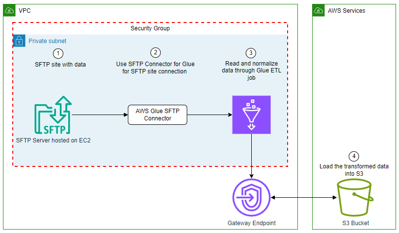
In this example, we walk through a typical migration solution, which is from the source HBase on HDFS cluster (Cluster A) to the target Amazon EMR HBase on S3 (Cluster B). The following diagram illustrates the solution architecture.

Solution architecture

To demonstrate the best practice recommended to the HBase migration process, the following are the detailed steps we will walk through, as shown in the preceding diagram.

Step	Activity	Description	Estimated time
1	Configure cluster A (Source HBase)	Modify the configuration of the source HBase cluster to prepare for subsequent snapshot exports	Less than 5 minutes
2	Create cluster B (Amazon EMR HBase on S3)	Create an EMR cluster with HBase on Amazon S3 as the migration target cluster	Less than 10 minutes
3	Configure replication	Configure replication from the source HBase cluster to Amazon EMR HBase, but do not start	Less than 1 minute
4	Pause service	Pause the service of the source HBase cluster	Less than 1 minute
5	Create snapshot	Create a snapshot for each table on the source HBase cluster	Less than 5 minutes
6	Resume service	Resume the service of the source HBase cluster	Less than 1 minute
7	Snapshot export and restore	Use snapshot to migrate data from the source HBase cluster to the Amazon EMR HBase cluster	Depends on the size of the table data volume
8	Start replication	Start the replication of the source HBase cluster to Amazon EMR HBase and synchronize incremental data	Depends on the size of the data accumulated during the snapshot export restore.
9	Test and verify	Test the and verify the Amazon EMR HBase

Solution walkthrough

In the preceding diagram and table, we have listed the operational steps of the solution. Next, we will elaborate the specific operations for each step shown in the preceding table.

1. Configure cluster A (source HBase)

When exporting a snapshot from the source HBase cluster to the Amazon EMR HBase cluster, you must modify the following settings on the source cluster to ensure the performance and stability of data transmission.

Configuration classification	Configuration item	Suggested value	Comment
core-site	`fs.s3.awsAccessKeyId`	Your AWS access key ID	The snapshot export takes a relatively long time. Without an access key and secret key, the snapshot export to Amazon S3 will encounter errors such as `com.amazon.aws.emr.hadoop.fs.shaded.com. amazonaws.SdkClientException:` Unable to load AWS credentials from any provider in the chain.
core-site	`fs.s3.awsSecretAccessKey`	Your AWS secret access key
yarn-site	`yarn.nodemanager.resource.memory-mb`	Half of a single core node RAM	The amount of physical memory, in MB, that can be allocated for containers.
yarn-site	`yarn.scheduler.maximum-allocation-mb`	Half of a single core node RAM	The maximum allocation for every container request at the ResourceManager in MB. Because snapshot export runs in the YARN Map Reduce task, it’s necessary to allocate sufficient memory to YARN to ensure transmission speed.

These values are set depending on the cluster resource, workload, and table data volume. The modification can be done using a web UI if available or by suing a standard configuration XML file. Restart the HBase service after the change is complete.

2. Create cluster B (EMR HBase on S3)

Use the following recommend settings to launch an EMR cluster:

Configuration classification	Configuration item	Suggested value	Comment
yarn-site	`yarn.nodemanager.resource.memory-mb`	20% of a single core node RAM	Amount of physical memory, in MB, that can be allocated for containers.
yarn-site	`yarn.scheduler.maximum-allocation-mb`	20% of a single core node RAM	The maximum allocation for every container request at the `ResourceManager` in MB. Because snapshot restore runs in the HBase, it’s necessary to allocate a small amount of small memory to YARN and leave sufficient memory to HBase to ensure restore.
hbase-env.export	`HBASE_MASTER_OPTS`	70% of a single core node RAM	Set the Java heap size for the primary HBase.
hbase-env.export	`HBASE_REGIONSERVER_OPTS`	70% of a single core node RAM	Set the Java heap size for the HBase region server.
hbase	`hbase.emr.storageMode`	S3	Indicates that HBase uses S3 to store data.
hbase-site	`hbase.rootdir`	<Your-HBase-Folder-on-S3>	Your HBase data folder on S3.

See Configure HBase for more details. Additionally, the default YARN configuration on Amazon EMR for each Amazon EC2 instance type can be found in Task configuration.

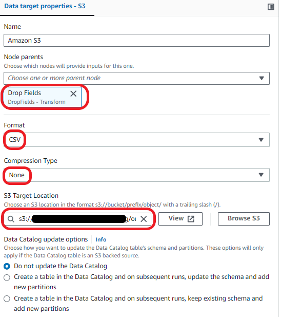
The configuration of our example is as shown in the following figure.

Instance group configurations

3. Config replication

Next, we configure the replication peer from the source HBase to the EMR cluster.

The operations include:

Create a peer.
Because the snapshot migration hasn’t been done, we start by disabling the peer.
Specify the table that requires replication for the peer.
Enable table replication.

Let’s use the table usertable as an example. The shell script is as follows:

MASTER_IP="<Master-IP>"
TABLE_NAME="usertable"
cat << EOF | sudo -u hbase hbase shell 2>/dev/null
add_peer 'PEER_$TABLE_NAME', CLUSTER_KEY => '$MASTER_IP:2181:/hbase'
disable_peer 'PEER_$TABLE_NAME'
enable_table_replication '$TABLE_NAME'
EOF

The result will like the following text.

hbase:001:0> add_peer 'PEER_usertable', CLUSTER_KEY => '<Master-IP>:2181:/hbase'
Took 13.4117 seconds 
hbase:002:0> disable_peer 'PEER_usertable'
Took 8.1317 seconds 
hbase:003:0> enable_table_replication 'usertable'
The replication of table 'usertable' successfully enabled
Took 168.7254 seconds

In this experiment, we’re using the table usertable as an example. If we have many tables that need to be configured for replication, we can use the following code:

MASTER_IP="<Master-IP>"

# Get all tables
TABLE_LIST=$(echo 'list' | sudo -u hbase hbase shell 2>/dev/null | sed -e '1,/TABLE/d' -e '/seconds/,$d' -e '/row/,$d')
# Iterate each table
for TABLE_NAME in $TABLE_LIST; do
# Add the operation
cat << EOF | sudo -u hbase hbase shell 2>/dev/null
add_peer 'PEER_$TABLE_NAME', CLUSTER_KEY => '$MASTER_IP:2181:/hbase'
disable_peer 'PEER_$TABLE_NAME'
enable_table_replication '$TABLE_NAME'
EOF
done

In the scripts of following steps, if you need to apply the operations for all tables, you can refer to the preceding code sample.

At this point, the status of the peer is Disabled, so replication won’t be started. And the data that needs to be synchronized from the source to the target EMR cluster will be backlogged at the source HBase cluster and won’t be synchronized to HBase on the EMR cluster.

After the snapshot restore (step 7) is completed on the HBase on Amazon EMR cluster, we can enable the peer to start synchronizing data.

If the source HBase version is 1.x, you must run the set_peer_tableCFs function. See HBase Cluster Replication.

4. Pause the service

To pause the service of the source HBase cluster, disable the HBase tables. You can use the following script:

sudo -u hbase bash /usr/lib/hbase/bin/disable_all_tables.sh 2>/dev/null

The result is shown in the following figure.

Disable all tables

After disabling all tables, observe the HBase UI to ensure that no background tasks are being run, and then stop any services accessing the source HBase. This will take 5-10 minutes.

The HBase UI is as shown in the following figure.

Check background tasks

5. Create a snapshot

Make sure the tables in the source HBase are disabled. Then, you can create a snapshot of the source. This process will take 1-5 minutes.

Let’s use the table usertable as an example. The shell script is as follows：

DATE=`date +"%Y%m%d"`
TABLE_NAME="usertable"
sudo -u hbase hbase snapshot create -n "${TABLE_NAME/:/_}-$DATE" -t ${TABLE_NAME} 2>/dev/null

You can check the snapshot with a script:

sudo -u hbase hbase snapshot info -list-snapshots 2>/dev/null

And the result is as shown in the following figure.

Create snapshot

6. Resume service

After the snapshot is successfully created on the source HBase, you can enable the tables and resume the services that access the source HBase. These operations take several minutes, so the total data unavailability time on the source HBase during the implementation (steps 3 to step 6) will be approximately 10 minutes.

The command to enable the table is as follows:

TABLE_NAME="usertable"
echo -e "enable '$TABLE_NAME'" | sudo -u hbase hbase shell 2>/dev/null

The result is shown in the following figure.

Enable table

At this point, you can write data to the source HBase, because the status of the replication peer is disabled, so the incremental data won’t be synchronized to the target cluster.

7. Snapshot export and restore

After the snapshot created in the source HBase, it’s time to export the snapshot to the HBase data directory on the target EMR cluster. The example script is as follows：

DATE=`date +"%Y%m%d"`
TABLE_NAME="usertable"
TARGET_BUCKET="<Your-HBase-Folder-on-S3>"
nohup sudo -u hbase hbase snapshot export -snapshot ${TABLE_NAME/:/_}-$DATE -copy-to $TARGET_BUCKET &> ${TABLE_NAME/:/_}-$DATE-export.log &

Exporting the snapshot will take from 10 minute to several hours to complete, depending on the amount of data to be exported. So we run it in the background. You can check the progress by using the yarn application -list command, as shown in the following figure.

Exporting snapshot process

As an example, if you’re using an HBase cluster with 20 r6g.4xlarge core nodes, it will take about 3 hours for 50 TB of data to be exported to Amazon S3 in same AWS Region.

After the snapshot export is completed at the source HBase, you can check the snapshot in the target EMR cluster using the following script:

sudo -u hbase hbase snapshot info -list-snapshots 2>/dev/null

The result is shown in the following figure.

Check snapshot

Confirm the snapshot name—for example, usertable-20240710 and run snapshot restore on the target EMR cluster using the following script.

TABLE_NAME="usertable"
SNAPSHOT_NAME="usertable-20240710"
cat << EOF | nohup sudo -u hbase hbase shell &> restore-snapshot.out &
disable '$TABLE_NAME'
restore_snapshot '$SNAPSHOT_NAME'
enable '$TABLE_NAME'
EOF

The snapshot restore will take from 10 minute to several hours to complete, depending on the amount of data to be restored, so we run it in the background. The result is as shown in the following figure.

Restore snapshot

You can check the progress of the restore through The Amazon EMR web interface for HBase, as shown in the following figure.

Check snapshot restore

From the Amazon EMR web interface for HBase, you can found it takes about 2 hours to run Clone Snapshot for a sample table with 50 TB of data, and then 1 additional hour to run . After these two stages, the snapshot restore is completed.

8. Start replication

After the snapshot restore is completed on the EMR cluster and the status of the table is set to enabled, you can enable HBase replication in the source HBase. The incremental data will be synchronized to the target EMR cluster.

In the source HBase, the example script is as follows:

TABLE_NAME="usertable"
echo -e "enable_peer 'PEER_$TABLE_NAME'" | sudo -u hbase hbase shell 2>/dev/null

The result is as shown in the following figure.

Enable peer

Wait for the incremental data to be synchronized from the source HBase to the HBase on EMR cluster. The time taken depends on the amount of data accumulated in the source HBase during the snapshot export and restore. In our example, it took about 10 minutes to complete the data synchronization.

You can check the replication status with scripts:

echo -e "status 'replication'" | sudo -u hbase hbase shell 2>/dev/null

The result is shown in the following figure.

Replication status

9. Test and verify

After incremental data synchronization is complete, you can start testing and verifying the results. You can use the same HBase API to access both the source and the target HBase clusters and compare the results.

To guarantee the data integrity, you can check the number of HBase table region and store files for the replicated tables from the Amazon EMR web interface for HBase, as shown in the following figure.

Check hbase region and store files

For small tables, we recommend using the HBase command to verify the number of records. After signing in to the primary node of the Amazon EMR using SSH, you can run the following command:

sudo -u hbase hbase org.apache.hadoop.hbase.mapreduce.RowCounter 'usertable'

Then, in the hbase.log file of the HBase log directory, find the number of records for the table usertable.

For large tables, you can use the HBase Java API to validate the row count in a range of row keys.

We provided sample Java code to implement this functionality. For example, we imported the demo data to usertable using the following script:

java -classpath hbase-utils-1.0-SNAPSHOT-jar-with-dependencies.jar HBaseAccess <Your-Zookeeper-IP> put 1000 20

The result is shown in the following figure.

Put demo data into HBase table

You can run the script multiple times to import enough demo data into the table, then you can use the following script to count the number of records where the value of Row Key is between user1000 and user5000, and the value of the column family:field0 is value0

java -classpath hbase-utils-1.0-SNAPSHOT-jar-with-dependencies.jar HBaseRowCounter <Your-Zookeeper-IP> usertable "user1000" "user1100" "family:field0" "value0"

The result is shown in the following figure.

HBase table row counter

You can run the same code on both the source HBase and the target Amazon EMR HBase to verify that the results are consistent. See complete code.

After these steps are complete, you can switch from the source HBase to the target Amazon EMR Hbase, completing the migration.

Clean up

After you’re done with the solution walkthrough, complete the following steps to clean up your resources:

Stop the Amazon EMR on EC2 cluster.
Delete the S3 bucket that stores the HBase data.
Stop the source HBase cluster, and release its related resource, for example, the Amazon EC2 cluster or resources provided by other vendors or cloud service providers.

Key challenges in HBase migration

In the previous sections, we have detailed the steps to implement HBase online migration through snapshots and replication for general scenario. Many customers’ scenarios may have some differences from the general scenario, and you need to make some modifications to the process steps in order to accomplish the migration.

HBase in the cloud doesn’t support snapshot

Many cloud providers have made modifications to the open source version of HBase, resulting in these versions of HBase not providing snapshot and replication functions. However, these cloud providers will provide data transfer tools for HBase, such as Lindorm Tunnel Service, that can be used to transfer HBase data to an HBase cluster with data on HDFS.

To deploy HBase on Amazon S3, you should follow the previous migration process as the best practice, using snapshot and replication techniques to migrate to an Amazon EMR environment. To solve the problem of HBase versions that don’t support snapshots and replication, you can create an HBase on HDFS as a jump or relay cluster, which can be used to synchronize the data from a source HBase to an HDFS-based HBase cluster, then migrate from the middle cluster to the target HBase on S3.

The following diagram illustrates the solution architecture.

Solution architecture for HBase in the cloud doesn’t support snapshot

You need to add three more steps in addition to the migration steps described previously.

Step	Activity	Description	Estimated time
1	Create Cluster B (EMR HBase on HDFS)	Create an EMR cluster with HBase on HDFS as the relay cluster.	Less than 10 minutes
2	Configure data transfer	Configure the data transfer from the outer HBase cluster to Amazon EMR HBase on HDFS and start the data transfer.	Less than 5 minutes
3	HBase migration (snapshot and replication)	Treat the outer HBase cluster as an application which writes data into the Amazon EMR HBase cluster, then you can use the steps in the previous scenario to complete the migration to Amazon EMR HBase on Amazon S3.

Single table with large amounts of data

During the migration process, if the amount of data in a single table in the source HBase (Cluster A) is too large—such as 10 TB or even 50TB—you must modify the target Amazon EMR HBase cluster (Cluster B) configuration to ensure that there are no interruptions during the migration process, especially during the snapshot restore on the Amazon EMR HBase cluster. After the snapshot restore is complete, you can rebuild the Amazon EMR HBase cluster (Cluster C).

The following diagram illustrates the solution architecture for handling a very large table.

Solution architecture for handling a very large table

The following are the steps.

Step	Activity	Description	Estimated time
1	Create Cluster B (EMR HBase on S3 for restore)	Create an EMR cluster with the required configuration for a large table snapshot restore.	Less than 10 minutes
2	HBase migration (snapshot and replication)	Consider the Amazon EMR HBase on Amazon S3 as the target cluster, then you can use the steps in the first scenario to complete the migration from the source HBase to the Amazon EMR HBase on S3.
3	Recreate Cluster C (EMR HBase on S3 for production)	After the migration is complete, Cluster B needs to be changed back to its previous configuration before migration. If it’s inconvenient to modify the parameters, you can use the previous configuration to recreate the EMR cluster (Cluster C).	Less than 15 minutes
4	Rebuild replication	After recreating the EMR cluster, if replication is still needed to synchronize the data, the replication from the source HBase cluster to the new EMR HBase cluster must be rebuilt. Before building the new EMR cluster, the write service on the source HBase cluster should be paused to avoid data loss on the Amazon EMR HBase.	Less than 1 minute

In Step 1, create cluster B (EMR HBase on S3 for restore), use the following configuration for snapshot restore. All time values are in milliseconds.

Configuration classification	Configuration item	Default value	Suggested value	Explanation
emrfs-site	`fs.s3.maxConnections`	1000	50000	The number of concurrent Amazon S3 connections that your applications need. The default value is 1000 and must be increased to avoid errors such as `com. amazon. ws. emr. hadoop. fs. shaded. com. amazonaws. SdkClientException: Unable to execute HTTP request: timeout waiting for connection from` pool.
hbase-site	`hbase.client.operation.timeout`	300000	18000000	Operation timeout is a top-level restriction that makes sure a blocking operation in a table will not be blocked for longer than the timeout.
hbase-site	`hbase.master.cleaner.interval`	60000	18000000	The default is to run HBase Clearer in 60,000 milliseconds, which will clear some files in the archive, resulting in an error that HFile cannot be found.
hbase-site	`hbase.rpc.timeout`	60000	18000000	This property limits how long a single RPC call can run before timing out.
hbase-site	`hbase.snapshot.master.timeout.millis`	300000	18000000	Timeout for the primary HBase for the snapshot procedure.
hbase-site	`hbase.snapshot.region.timeout`	300000	18000000	Timeout for region servers to keep threads in a snapshot request pool waiting.
hbase-site	`hbase.hregion.majorcompaction`	604800000	0	Default is 604,800,000 ms (1 week). Set to 0 to disable automatic triggering of compaction. Note that because of the change to manual triggering, you must make compaction one of the daily operation and maintenance tasks, and run it during periods of low activity to avoid impacting production. The following is the compaction script: `echo -e "major_compact '$TABLE_NAME'" \| sudo -u hbase hbase shell`

Adjust the suggested values based on the amount of table data, which requires conducting some experiments to determine the values to be used in the final migration plan.

Before you recreate a new EMR cluster in the production environment, disable the HBase table on the active EMR cluster. The command line is as follows:

sudo -u hbase bash /usr/lib/hbase/bin/disable_all_tables.sh 2>/dev/null
echo -e "flush 'hbase:meta'" | sudo -u hbase hbase shell 2>/dev/null

Wait for the command to execute successfully and terminate the current EMR cluster (Cluster B). Now the HBase data is kept in Amazon S3; create a new EMR cluster (Cluster C) with the previous configuration before migration, and specify HBase date folder on S3 to be the same as Cluster B.

Using Bucket Cache to improve read performance

To enhance HBase’s read performance, one of most effective method involves caching data. HBase uses BlockCache to implement caching mechanisms for the region server. Currently, HBase provides two different BlockCache implementations to cache data read from HDFS: the default on-heap LruBlockCache and the BucketCache, which is usually off-heap. Bucket cache is the most used method.

BucketCache can be deployed in offheap, file, or mmaped file mode. These three working modes are the same in terms of memory logical organization and caching process; however, the final storage media corresponding to these three working modes are different, that is, the IOEngine is different.

We recommend that customers use BucketCache in file mode, because the default storage type of Amazon Elastic Block Store (Amazon EBS) in Amazon EMR is SSD. You can put all hot data into BucketCache, which is on Amazon EBS. You can then determine the file size used by BucketCache based on the volume of hot data.

The following are the HBase configurations for BucketCache.

Configuration classification	Configuration item	Suggested value	Explanation
emrfs-site	`hbase.bucketcache.ioengine`	files:`/mnt1/hbase/cache_01.data`	Where to store the contents of the bucket cache. You can use offheap, file, files, mmap, or pmem. If a file or files, set it to files. Note that some earlier Amazon EMR versions can only support using one file per core node.
hbase-site	`hbase.bucketcache.persistent.path`	file:`/mnt1/hbase/cache.meta`	The path to store the metadata of the bucket cache, used to recover the cache during startup.
hbase-site	`hbase.bucketcache.size`	Depends on the hot data volume be cached	The capacity in MBs of BucketCache for each core node. If you use multiple cache files, then this size is the sum of the capacities of multiple files.
hbase-site	`hbase.rs.prefetchblocksonopen`	TRUE	Whether the server should asynchronously load all the blocks when a store file is opened (data, metadata, and index). Note that enabling this property contributes to the time the region server takes to open a region and therefore initialize.
hbase-site	`hbase.rs.cacheblocksonwrite`	TRUE	Whether an HFile block should be added to the block cache when the block is finished.
hbase-site	`hbase.rs.cachecompactedblocksonwrite`	TRUE	Whether to cache compressed blocks during writing.

More configuration instructions for BucketCache would refer to Configuration properties.

We provided sample Java code to test HBase read performance. In the Java code, we use the putDemoData method to write test data to the table usertable, ensuring that the data is evenly distributed across HBase table regions, and then use the getDemoData method to read the data.

We tested three scenarios: HBase data stored on HDFS, on Amazon S3 without using BucketCache, and on S3 using BucketCache. To ensure that the written data isn’t cached in the first two scenarios, the cache can be cleared by restarting the the region servers.

We tested on the EMR HBase cluster, which has 10 r6g. 2xlarge core nodes. The command is as follows:

java -classpath hbase-utils-1.0-SNAPSHOT-jar-with-dependencies.jar HBaseAccess <Your-Zookeeper-IP> get 20 100

The result is shown in the following figure.

Read HBase table

Benchmark results and key learning

For the three scenarios, we use 100 HBase record row keys as input, ensure these row keys distributed evenly in HBase table regions, we call the API consecutively with 20 times, 50 times, and 100 times, and we got the time cost result as the following figure. We found the read latency is the shortest when the data is on S3 and using BucketCache.

Read performance

Above, we introduced four migration scenarios. In migration processes in production, we’ve gained invaluable knowledge and experience. We’re sharing the results here for you to use as best practices and a recommended run book.

Configuration parameters

In the configurations provided earlier, some are necessary for BucketCache settings while others mitigate known errors to reduce the snapshot duration. For example, the parameter hbase.snapshot.master.timeout.millis is related to the HBASE-14680 issue. It’s advisable to retain these configurations as much as possible throughout the migration process.

Version choice

When migrating to Amazon EMR and choosing a suitable HBase version, it is recommended to select a more recent minor version and patch version, while keeping the major version unchanged. That is to say:

If the source HBase is version 1.x, we recommend using EMR 5.36.1, whose HBase version is 1.4.13, because the HBase 1.x API is compatible and won’t require you to make code changes.
If the source HBase is version 2.x, we recommend using EMR 6.15.0, which has an HBase of 2.4.17.

The HBase API under the same major version can be universal. See HBase Version to learn more.

Allocating enough space

HDFS needs to leave enough space when exporting snapshots, it depends on the data volume. Data will be moved to the archive, causing double storage is needed for the table.

Replication

At present, there is compatibility problem if replication and WAL compression are used together. If you are using replication, set the hbase.regionserver.wal.enablecompression property to false. See HBASE-26849 for more information.

By default, replication in HBase is asynchronous, as the write-ahead log (WAL) is sent to another cluster in the background. This implies that when using replication for data recovery, some data loss may occur. Additionally, there is a potential for data overwrite conflicts when concurrently writing the same record within a short time frame. However, HBase v2.x introduces synchronous replication as a solution to this issue. For more details, refer to the Serial Replication documentation.

Disk type for BucketCache

Because BucketCache uses a portion of Amazon EBS IO and throughput to synchronize data, it’s recommended to choose Amazon EBS gp3 volumes for their higher IOPS and throughput.

Response latency when accessing to HBase

Users sometimes face the issue of high response latency from their Hbase on EMR clusters using API calls or the HBase shell tool.

In our testing, we found that the communication between HMaster and RegionServer takes an unusually long time to resolve through DNS. You can reduce latency by adding the host name and IP mapping to the /etc/hosts file in the HBase client host.

Conclusion

In this post, we used the results of real-world migration cases to introduce the process of migrating HBase to Amazon EMR HBase using HBase snapshot and replication and the deployment mode of HBase on Amazon S3. We included how to resolve challenges, such as how to configure the cluster to make the migration process smoother when migrating a single large table, or how to use BucketCache to improve reading performance. We also described techniques for testing performance.

We encourage you to migrate HBase to Amazon EMR HBase. For more information about HBase migration, see Amazon EMR HBase best practices.

About the Authors

Dalei Xu is a Analytics Specialist Solution Architect at Amazon Web Services, responsible for consulting, designing, and implementing AWS data analytics solutions. With over 20 years of experience in data-related work, proficient in data development, migration to AWS, architecture design, and performance optimization. Hoping to promote AWS data analytics services to more customers, achieving a win-win situation and mutual growth with customers.

Zhiyong Su is a Migration Specialist Solution Architect at Amazon Web Services, primarily responsible for cloud migration or cross-cloud migration for enterprise-level clients. Has held positions such as R&D Engineer, Solutions Architect, and has years of practical experience in IT professional services and enterprise application architecture.

Shijian Tang is a Analytics Specialist Solution Architect at Amazon Web Services.

AWS Weekly Roundup: What’s App, AWS Lambda, Load Balancers, AWS Console, and more (Oct 14, 2024).

2024-10-14 Sébastien Stormacq

Post Syndicated from Sébastien Stormacq original https://aws.amazon.com/blogs/aws/aws-weekly-roundup-whats-app-aws-lambda-load-balancers-aws-console-and-more-oct-14-2024/

Last week, AWS hosted free half-day conferences in London and Paris. My colleagues and I demonstrated how developers can use generative AI tools to speed up their design, analysis, code writing, debugging, and deployment workflows. These events were held at the GenAI Lofts. These lofts are open until October 25 (London) and November 5 (Paris). They will be packed with events, conferences, workshops, and meetups. If you’re around, be sure to check the agenda (London, Paris).

Veliswa live coding on stage at NGDE Day London

Our well-known AWS News blog co-author Veliswa did an amazing demo. She live-coded a Duolingo-like app from scratch, just using suggestions and reviews from Amazon Q Developer.

Now, let’s turn to other exciting news in the AWS universe from last week.

Last week’s launches
Here are some launches that got my attention:

Bring your conversations to WhatsApp — AWS has added support for What’sApp to AWS End User Messaging, so developers can reach users on WhatsApp with multimedia and interactive messaging options. This feature integrates with SMS and push notifications already available. Developers can get started quickly using AWS Management Console.

Amazon Redshift data sharing with data lake tables — This offers a secure and convenient way to share live data lake tables across different Amazon Redshift warehouses. Data sharing of data lake tables in AWS Glue Data Catalog provides live access to the data, so you always see the most up-to-date and consistent information as it’s updated in the data lake.

Zonal shift and zonal autoshift for cross zoned Network Load Balancer — Network Load Balancer (NLB) now supports the Amazon Application Recovery Controller zonal shift and zonal autoshift features on load balancers that are enabled across zones. With Zonal shift, you can quickly shift traffic away from an impaired Availability Zone and recover from events such as bad application deployment and gray failures. Zonal autoshift safely and automatically shifts your traffic away from an Availability Zone when AWS identifies a potential impact to it.

Console to Code to generate infrastructure as a service code — This is by far my favorite launch of the week. Console to Code makes it simple, fast, and cost-effective to move from prototyping in the AWS Management Console to building code for production deployments. You can generate code for their console actions in their preferred format with a single click. The generated code helps you get started and bootstrap your automation pipelines for tasks. Console to Code is powered by Amazon Q Developer.

A new getting started experience for AWS CodePipeline — AWS Data Pipeline introduces a simplified and new getting started experience so you can quickly create new pipelines. When you create a new pipeline using the CodePipeline console, you can now select from a list of pipeline templates across build, automation, and deployment use cases. After selecting a pipeline template, you will be prompted to enter values for the action configuration fields in the pipeline definition, and completing the process will render a fully configured pipeline that’s ready to run.

AWS Lambda detects and stops recursive loops between Lambda and Amazon S3 — Lambda recursive loop detection can now automatically detect and stop recursive loops between AWS Lambda and Amazon Simple Storage Service (Amazon S3). Lambda recursive loop detection, which is enabled by default, is a preventative guardrail that automatically detects and stops recursive invocations between Lambda and other supported services, preventing unintended usage and billing from runaway workloads.

Amazon MemoryDB for Valkey — Amazon MemoryDB for Redis is a fully managed, Valkey– and Redis OSS-compatible database service, which provides multi-AZ durability, microsecond read and single-digit millisecond write latency, and high throughput. It is ideal for use cases such as caching, leaderboards, and session stores. With MemoryDB for Valkey, you can benefit from a fully managed experience built on open-source technology while using the security, operational excellence, and reliability that AWS provides. MemoryDB for Valkey also delivers the fastest vector search performance at the highest recall rates among popular vector databases on AWS.

Amazon Polly adds four wew English voices for the generative engine and expands to three Regions — Polly is a managed service that turns text into lifelike speech, so you can create applications that talk and to build speech-enabled products depending on your business needs. The generative engine is the most advanced Amazon Polly text-to-speech (TTS) model. With this launch, we add a variety of new synthetic generative English voices to the Amazon Polly portfolio: an Australian English voice Olivia and three US English voices Joanna, Danielle, and Stephen. These voices have more natural pronunciation and prosody. You can use this high-tier product in various industries and for different purposes such as education, publishing, or marketing.

For a full list of AWS announcements, be sure to keep an eye on the AWS What’s New Feed page.

Upcoming AWS events
Check your calendars and sign up for these AWS events:

AWS Cloud Day Prague — Join us for a free technical conferences in Prague on October 23. I will be there and share with attendees “The Art of Transforming a Foundation Model into a Domain Expert”. Be sure to register today!

Innovate Migrate, Modernize, and Build — Whether you are new to the cloud or an experienced user, you will learn something new at AWS Innovate. This is a free online conference. Register for a time and region convenient to North America (October 15), or Europe, Middle East & Africa (October 24).

AWS Community Days — Join community-led conferences featuring technical discussions, workshops, and hands-on labs led by expert AWS users and industry leaders from around the world. Don’t miss out on the AWS Community Days happening on October 19 in Vadodara, Spain, and Guatemala.

AWS re:Invent 2024 — Registration is now open for the annual tech extravaganza, taking place December 2 – 6 in Las Vegas. Beside recording podcast episodes, I will present three sessions:

CMP410 | Accelerate testing cycles of CI/CD pipelines with EC2 Mac instances (with Vishal)
DEV301 | The art of transforming foundation models into domain experts (with Gregory)
DEV334 | Swift, server-side, serverless

There are just a few seats left for these three sessions, so be sure to book your seat today!

Browse more upcoming AWS led in-person and virtual events and developer-focused events.

That’s all for this week. Check back next Monday for another Weekly Roundup!

— seb

This post is part of our Weekly Roundup series. Check back each week for a quick roundup of interesting news and announcements from AWS!

Take manual snapshots and restore in a different domain spanning across various Regions and accounts in Amazon OpenSearch Service

2024-10-11 Madhan Kumar Baskaran

Post Syndicated from Madhan Kumar Baskaran original https://aws.amazon.com/blogs/big-data/take-manual-snapshots-and-restore-in-a-different-domain-spanning-across-various-regions-and-accounts-in-amazon-opensearch-service/

Snapshots are crucial for data backup and disaster recovery in Amazon OpenSearch Service. These snapshots allow you to generate backups of your domain indexes and cluster state at specific moments and save them in a reliable storage location such as Amazon Simple Storage Service (Amazon S3).

Snapshots play a critical role in providing the availability, integrity and ability to recover data in OpenSearch Service domains. By implementing a robust snapshot strategy, you can mitigate risks associated with data loss, streamline disaster recovery processes and maintain compliance with data management best practices.

This post provides a detailed walkthrough about how to efficiently capture and manage manual snapshots in OpenSearch Service. It covers the essential steps for taking snapshots of your data, implementing safe transfer across different AWS Regions and accounts, and restoring them in a new domain. This guide is designed to help you maintain data integrity and continuity while navigating complex multi-Region and multi-account environments in OpenSearch Service.

Refer to this developer guide to understand more about index snapshots

Understanding manual snapshots

Manual snapshots are point-in-time backups of your OpenSearch Service domain that are initiated by the user. Contrary to automated snapshots, which are taken on a regular basis in accordance with the specified retention policy by OpenSearch Service, manual snapshots give you the ability to take backups whenever required, whether for the full cluster or for individual indices. This is particularly useful when you want to preserve a specific state of your data for future reference or before implementing significant changes to your domain.

Snapshots are not instantaneous. They take time to complete and don’t represent perfect point-in-time views of the domain. While a snapshot is in progress, you can still index documents and make other requests to the domain, but new documents and updates to existing documents generally aren’t included in the snapshot. The snapshot includes primary shards as they existed when you initiate the snapshot process.

The following are some scenarios where manual snapshots play an important role:

Data recovery – The primary purpose of snapshots, whether manual or automated, is to provide a means of data recovery in the event of a failure or data loss. If something goes wrong with your domain, you can restore it to a previous state using a snapshot.
Migration – Manual snapshots can be useful when you want to migrate data from one domain to another. You can create a snapshot of the source domain and then restore it on the target domain.
Testing and development – You can use snapshots to create copies of your data for testing or development purposes. This allows you to experiment with your data without affecting the production environment.
Backup control – Manual snapshots give you more control over your backup process. You can choose exactly when to create a snapshot, which can be useful if you have specific requirements that are not met by automated snapshots.
Long-term archiving – Manual snapshots can be kept for as long as you want, which can be useful for long-term archiving of data. Automated snapshots, on the other hand, are often deleted after a certain period of time.

Solution overview

The following sections outline the procedure for taking a manual snapshot and then restoring it in a different domain, spanning across various Regions and accounts. The high-level steps are as follows:

Create an AWS Identity and Access Management (IAM) role and user.
Register a manual snapshot repository.
Take manual snapshots.
Set up S3 bucket replication.
Create an IAM role and user in the target account.
Add a bucket policy.
Register the repository and restore snapshots in the target domain.

Prerequisite

This post assumes you have the following resources set up:

An active and running OpenSearch Service domain.
An S3 bucket to store the manual snapshots of your OpenSearch Service domain. The bucket has to be in the same Region where the OpenSearch Service domain is hosted.

Create an IAM role and user

Complete the following steps to create your IAM role and user:

Create an IAM role to grant permissions to OpenSearch Service. For this post, we name the role TheSnapshotRole.
Create a new policy using the following code and attach it to the role to allow access to the S3 bucket.

{
  "Version": "2012-10-17",
  "Statement": [
    {
      "Action": [
        "s3:ListBucket"
      ],
      "Effect": "Allow",
      "Resource": [
        "arn:aws:s3:::s3-bucket-name"
      ]
    },
    {
      "Action": [
        "s3:GetObject",
        "s3:PutObject",
        "s3:DeleteObject",
        "iam:PassRole"
      ],
      "Effect": "Allow",
      "Resource": [
        "arn:aws:s3:::s3-bucket-name/*"
      ]
    }
  ]
}

Edit the trust relationship of TheSnapshotRole to specify OpenSearch Service in the Principal statement, as shown in the following example. Under the Condition block, we recommend that you use the aws:SourceAccount and aws:SourceArn condition keys to protect yourself against the confused deputy problem. The source account is the owner and the source ARN is the ARN of the OpenSearch Service domain.

{
  "Version": "2012-10-17",
  "Statement": [
    {
      "Sid": "",
      "Effect": "Allow",
      "Principal": {
        "Service": "es.amazonaws.com"
      },
      "Action": "sts:AssumeRole",
      "Condition": {
        "StringEquals": {
          "aws:SourceAccount": "account-id"
        },
        "ArnLike": {
          "aws:SourceArn": "arn:aws:es:region:account-id:domain/domain-name"
        }
      }
    }
  ]
}

Generate an IAM user to register the snapshot repository. For this post, we name the user TheSnapUser.
To register a snapshot repository, you need to pass TheSnapshotRole to OpenSearch Service. You also need access to the es:ESHttpPut To grant both of these permissions, attach the following policy to the IAM role whose credentials are being used to sign the request.

{
  "Version": "2012-10-17",
  "Statement": [
    {
      "Effect": "Allow",
      "Action": "iam:PassRole",
      "Resource": "arn:aws:iam::123456789012:role/TheSnapshotRole"
    },
    {
      "Effect": "Allow",
      "Action": "es:ESHttpPut",
      "Resource": "arn:aws:es:region:123456789012:domain/domain-name/*"
    }
  ]
}

Register a manual snapshot repository

Complete the following steps to map the snapshot role and the user in OpenSearch Dashboards (if using fine-grained access control):

Navigate to the OpenSearch Dashboards endpoint connected to your OpenSearch Service domain.
Sign in with the admin user or a user with the security_manager role
From the main menu, choose Security, Roles, and select the manage_snapshots role
Choose Mapped users, then choose Manage mapping.
Add the ARN of TheSnapshotRole for Backend role and the ARN of TheSnapUser for User:
1. arn:aws:iam::123456789123:role/TheSnapshotRole
2. arn:aws:iam::123456789123:user/TheSnapUser
Choose Map and confirm the user and role shows up under Mapped users.
To register a snapshot repository, send a PUT request to the OpenSearch Service domain endpoint through an API platform like Postman or Insomnia. For more details, see Registering a manual snapshot repository.

Note: While using Postman or Insomnia to run the API calls mentioned throughout this blog, choose AWS IAM v4 as the authentication method and input your IAM credentials in the Authorization section. Ensure you use the credentials of an OpenSearch user who has the ‘all_access’ OpenSearch role assigned on the domain.

curl -XPUT domain-endpoint/_snapshot/my-snapshot-repo-name
{
  "type": "s3",
  "settings": {
    "bucket": "s3-bucket-name",
    "region": "region",
    "role_arn": "arn:aws:iam::123456789012:role/TheSnapshotRole"
  }
}

If your domain resides within a virtual private cloud (VPC), you must be connected to the VPC for the request to successfully register the snapshot repository. Accessing a VPC varies by network configuration, but likely involves connecting to a VPN or corporate network. To check that you can reach the OpenSearch Service domain, navigate to https://<your-vpc-domain.region>.es.amazonaws.com in a web browser and verify that you receive the default JSON response.

Take manual snapshots

Taking a snapshot isn’t possible if another snapshot is currently in progress. The Ultrawarm storage tier migration process also utilizes snapshots to move data between hot and warm storage, running this process in the background. Additionally, automated snapshots are taken based on the schedule configured for the cluster by the service. See Protecting data with encryption for protecting your Amazon S3 data.

To verify, run the following command

curl -XGET 'domain-endpoint/_snapshot/_status

After you confirm no snapshot is running, run the following command to take a manual snapshot

curl -XPUT 'domain-endpoint/_snapshot/repository-name/snapshot-name

Run the following command to verify the state of all snapshots of your domain

curl -XGET 'domain-endpoint/_snapshot/repository-name/_all?pretty

Set up S3 bucket replication

Before you start, have the following in place:

Locate the destination bucket where the data will be replicated. If you don’t have one, create a new S3 bucket in a distinct region, separate from the region of the source bucket.
To allow access to objects in this bucket by other AWS accounts (because the destination OpenSearch Service domain is in a different account), you need to enable access control lists (ACLs) on the bucket. ACLs will be used to specify and manage access permissions for the bucket and its objects.

Complete the following steps to set up S3 bucket replication. For more information, see Walkthroughs: Examples for configuring replication.

On the Amazon S3 console, choose Buckets in the navigation pane.
Choose the bucket you want to replicate (the source bucket with snapshots).
On the Management tab, choose Create replication rule.
Replication requires versioning to be enabled for the source bucket, so choose Enable bucket versioning and enable versioning.
Specify the following details:
1. For Rule ID, enter a name for your rule.
2. For Status, choose Enabled.
3. For Rule scope, specify the data to be replicated.
4. For Destination S3 bucket, enter the target bucket name where the data will be replicated.
5. For IAM role, choose Create new role.
Choose Save.
In the Replicate existing objects pop-up window, select Yes, replicate existing objects to start replication.
Choose Submit.

You will see a new active replication rule in the replication table on the Management tab of the source S3 bucket.

Create an IAM role and user in the target account

Complete the following steps to create your IAM role and user in the target account.

Create an IAM role to grant permissions to the target OpenSearch Service. For this post, name the role DestinationSnapshotRole.
Create a new policy using the following code and attach it to the role DestinationSnapshotRole to allow access to the target S3 bucket

{
  "Version": "2012-10-17",
  "Statement": [
    {
      "Action": [
        "s3:ListBucket"
      ],
      "Effect": "Allow",
      "Resource": [
        "arn:aws:s3:::s3-bucket-name" -> Replicated s3 bucket
      ]
    },
    {
      "Action": [
        "s3:GetObject",
        "s3:PutObject",
        "s3:DeleteObject",
        "iam:PassRole"
      ],
      "Effect": "Allow",
      "Resource": [
        "arn:aws:s3:::s3-bucket-name/*" -> Replicated s3 bucket 
      ]
    }
  ]
}

Edit the trust relationship of DestinationSnapshotRole to specify OpenSearch Service in the Principal statement as shown in the following example.

{
  "Version":"2012-10-17",
  "Statement":[
    {
      "Sid":"",
      "Effect":"Allow",
      "Principal":{
        "Service":"es.amazonaws.com"
      },
      "Action":"sts:AssumeRole",
      "Condition":{
        "StringEquals":{
          "aws:SourceAccount":"account-id" -> Target Account
        },
        "ArnLike":{
          "aws:SourceArn":"arn:aws:es:region:account-id:domain/domain-name/*" -> Target OpenSearch Domain
        }
      }
    }
  ]
}

Generate an IAM user to register the snapshot repository. For this post, name the user DestinationSnapUser.
To register a snapshot repository, you need to pass DestinationSnapshotRole to OpenSearch Service. You also need access to the es:ESHttpPut To grant both of these permissions, attach the following policy to the IAM role whose credentials are being used to sign the request

{
  "Version":"2012-10-17",
  "Statement":[
    {
      "Effect":"Allow",
      "Action":"iam:PassRole",
      "Resource":"arn:aws:iam::123456789012:role/DestinationSnapshotRole"
    },
    {
      "Effect":"Allow",
      "Action":"es:ESHttpPut",
      "Resource":"arn:aws:es:region:123456789012:domain/domain-name/*" -> Target OpenSearch Domain
    }
  ]
}

Complete the following steps to map the snapshot role and user in the target OpenSearch Dashboards (if using fine-grained access control).

Navigate to the OpenSearch Dashboard’s endpoint connected with your OpenSearch Service domain.
Sign in with the admin user or a user with the security_manager role
From the main menu, choose Security, Roles, and choose the manage_snapshots role
Choose Mapped users, then choose Manage mapping.
Add the ARN of TheSnapshotRole for Backend role and the ARN of TheSnapUser for User:
1. arn:aws:iam::123456789123:role/DestinationSnapshotRole
2. arn:aws:iam::123456789123:user/DestinationSnapUser
Choose Map and confirm the user and role shows up under Mapped users.

Add a bucket policy

In the destination S3 bucket details page, on the Permissions tab, choose Edit, then add the following bucket policy. This policy allows the target OpenSearch Service domain from another AWS account to access the snapshot created by a different AWS account.

{
  "Version":"2012-10-17",
  "Id":"Policy1568001010746",
  "Statement":[
    {
      "Sid":"Stmt1568000712531",
      "Effect":"Allow",
      "Principal":{
        "AWS":"arn:aws:iam::Account B:role/cross" -> DestinationSnapshotRole
      },
      "Action":"s3:*",
      "Resource":"arn:aws:s3:::snapshot"
    },
    {
      "Sid":"Stmt1568001007239",
      "Effect":"Allow",
      "Principal":{
        "AWS":"arn:aws:iam::Account B:role/cross" -> DestinationSnapshotRole
      },
      "Action":[
        "s3:GetObject",
        "s3:PutObject",
        "s3:DeleteObject"
      ],
      "Resource":"arn:aws:s3:::snapshot/*"
    }
  ]
}

Register the repository and restore snapshots in the target domain

To complete this step, you need an active and running OpenSearch Service domain in the target account.

Identify the snapshot you want to restore. Make sure all settings for this index, such as custom analyzer packages or allocation requirement settings, and data are compatible with the domain. Then complete the following steps

To register the repository in the target OpenSearch Service domain, run the following command.

curl -XPUT domain-endpoint/_snapshot/my-snapshot-repo-name
{
  "type": "s3",
  "settings": {
    "bucket": "s3-bucket-name",
    "region": "region",
    "role_arn": "arn:aws:iam::123456789012:role/DestinationSnapshotRole"
  }
}

After you register the repository, run the following command to see all snapshots.

curl -XGET 'domain-endpoint/_snapshot/repository-name/_all?pretty

To restore a snapshot, run the following command.

curl -XPOST 'domain-endpoint/_snapshot/repository-name/snapshot-name/_restore

Alternately, you might want to restore all indexes except the dashboards and fine-grained access control indexes.

curl -XPOST 'domain-endpoint/_snapshot/repository-name/snapshot-name/_restore' \
-d '{"indices": "-.kibana*,-.opendistro*"}' \
-H 'Content-Type: application/json'

Sign in to OpenSearch Dashboards connected to the target OpenSearch Service domain and run the following command to check if the data is getting restored.

curl -XGET _cat/indices?v

Run the following recovery command to check the progress of the restore operation.

curl -XGET _cat/recovery?v

Troubleshooting

This re:Post article addresses the majority of common errors that arise when attempting to restore a manual snapshot, along with effective solutions to resolve them.

Conclusion

In this post, we presented a procedure for taking manual snapshots and restoring them in OpenSearch Service. With manual snapshots, you have the power to manage your data backups, preserving key moments in time, confidently experimenting with domain modifications, and protecting against any data loss. Additionally, being able to restore snapshots across various domains, Regions, and accounts enables a new degree of data portability and flexibility, giving you the freedom to better manage and optimize your domains.

With great data protection comes great innovation. Now that you’re equipped with this knowledge, you can explore the endless possibilities that OpenSearch Service offers, confident in your ability to secure, restore, and thrive in the dynamic world of cloud-based data analytics and management.

See blog post to understand how to use snapshot management policies to manage automated snapshot in OpenSearch Service.

If you have feedback about this post, submit it in the comments section. If you have questions about this post, start a new thread on the Amazon OpenSearch Service forum or contact AWS Support.

Stay tuned for more exciting updates and new features in Amazon OpenSearch Service.

About the authors

Madhan Kumar Baskaran works as a Search Engineer at AWS, specializing in Amazon OpenSearch Service. His primary focus involves assisting customers in constructing scalable search applications and analytics solutions. Based in Bellevue, Washington, Madhan has a keen interest in data engineering and DevOps.

Priyanshi Omer is a Customer Success Engineer at AWS OpenSearch, based in Bengaluru. Her primary focus involves assisting customers in constructing scalable search applications and analytics solutions. She works closely with customers to help them migrate their workloads and aids existing customers in fine-tuning their clusters to achieve better performance and cost savings. Outside of work, she enjoys spending time with her cats and playing video games

How CyberArk is streamlining serverless governance by codifying architectural blueprints

2024-10-11 Anton Aleksandrov

Post Syndicated from Anton Aleksandrov original https://aws.amazon.com/blogs/architecture/how-cyberark-is-streamlining-serverless-governance-by-codifying-architectural-blueprints/

This post was co-written with Ran Isenberg, Principal Software Architect at CyberArk and an AWS Serverless Hero.

Serverless architectures enable agility and simplified cloud resource management. Organizations embracing serverless architectures build robust, distributed cloud applications. As organizations grow and the number of development teams increases, maintaining architectural consistency, standardization, and governance across projects becomes crucial.

In this post, you will discover how CyberArk, a leading identity security company, efficiently implements serverless architecture governance, reduces duplicative efforts, and saves months of development time by codifying architectural blueprints. This approach helps to prevent redundant efforts and promotes uniform architectural standards, facilitating the seamless adoption of organizational best practices and governance across diverse teams.

Overview

The risk of duplicative efforts and architectural inconsistencies is particularly pronounced in large organizations, especially for requirements unrelated to specific business domains owned by individual teams. Diverse approaches to Infrastructure-as-Code, CI/CD, observability, and security can lead to inconsistent implementations across teams. Application developers should focus on delivering business value efficiently, rather than navigating the complexities of building and operating distributed architectures while adhering to organizational best practices. To achieve this, you need an approach that empowers developers and provides guardrails to ensure vetted architectural patterns are consistently applied. This solution should enable accelerated delivery without sacrificing agility and innovation.

Some organizations implement internal wiki consolidating architectural guidance. While well-intentioned, relying solely on documentation assumes development teams diligently follow the guidelines, which often requires manual validation and limits scalability. To overcome this limitation, organizations should adopt a scalable approach that codifies, automates, and promotes architectural best practices. This mechanism allows developers to focus on delivering business-domain value and drives standardized operational excellence, governance, and organizational policies adherence.

Introducing serverless blueprints

CyberArk engineering team had over 900 developers. It was looking for ways to ensure they build their serverless services based on vetted architectural and security best practices with fully automated governance controls enforcement. The solution came in the form of codified architecture blueprints and automated tooling.

Serverless architectures are composed using loosely coupled services, integrated based on the application requirements. Application developers use IaC tools such as AWS CDK and HashiCorp Terraform to define their serverless architectures and integration patterns. CyberArk has augmented the IaC with governance tools, such as cdk-nag, AWS Config, and AWS Control Tower. With these complementary tools in place, they’ve built serverless blueprints which include architectural definitions based on organizational best practices, as well as automatically applied governance controls

To illustrate this, consider a simple serverless architecture pattern. In this common pattern, an SQS queue serves as the event source for a Lambda function, which parses incoming messages and updates an Amazon S3 bucket.

Figure 1. A simple serverless architecture with SQS Queue, Lambda function, and S3 Bucket

While this pattern seems simple, turning it into an enterprise-ready service requires additional effort. You must consider aspects like resiliency, security, governance, observability, and coding best practices. Let’s examine several examples codified in architectural blueprints at CyberArk.

Error-handling best practices

Your services should be resilient. Retries can help to overcome occasional network hiccups, but you also need to handle scenarios when your function consistently fails to process particular messages (known as poison message) – for example, because of a code bug. This can lead to endless processing loops, data loss, and potential extra charges. To address this, a blueprint can implement a failure handling mechanism with a dead letter queue, alerting, and redrive. This pattern is straightforward to implement and adds extra resiliency to your architecture. It is also generic and does not contain any business domain code. This is a typical example of an architectural pattern that can be codified in a blueprint and reused across development teams.

Figure 2. The simple serverless architecture with added resiliency best practices

Security best practices

Another example is securing S3 buckets. Organizations must enforce S3 security best practices, such as enabling access logs, blocking public access, and enabling encryption at rest. Codifying these guardrails in architectural blueprints adds an extra layer that allows your developers to comply with organization standards without having to explicitly implement adherence to each best practice and policy on their own.

Figure 3. The simple serverless architecture with added security best practices

The following code snippet uses AWS CDK to create an S3 bucket with common best practices:

Enables bucket versioning on production environments only to save costs in non-production environments
Enforces data encryption with AWS-managed keys.
Blocks all public access
Enforces SSL to block all non-secure-transport access
Enables access logs

def _create_bucket(self, server_access_logs_bucket: s3.Bucket, is_production_env: bool) -> s3.Bucket:
    # Create an S3 bucket with AWS-managed keys encryption
    bucket = s3.Bucket(
        self,
        constants.BUCKET_NAME,
        versioned=True if is_production_env else False,
        encryption=s3.BucketEncryption.S3_MANAGED,
        block_public_access=s3.BlockPublicAccess.BLOCK_ALL,
        enforce_ssl=True,
        server_access_logs_bucket=server_access_logs_bucket, 
        # redacted
    )

Additional security best practices you can codify in your blueprints include the principle of least privilege access, VPC-attachment, and code signing for sensitive Lambda functions, and using KMS keys for encryption.

Lambda best practices

Your Lambda functions are another example of where blueprints can help. By providing a function blueprint implementing the baseline for capabilities like observability, idempotency, and batch processing out-of-the-box, you enable developers to focus on their business domain code.

Figure 4. Layered view of a Lambda function in CyberArk’s serverless architecture blueprint

CyberArk embeds Powertools for AWS Lambda, a toolkit that implements serverless best practices to increase developer velocity, into their blueprints. The following code snippets embed Powertools for enabling enhanced observability and implementing batch processing.

# CDK code
lambda_function = lambda.Function(
    environment={
        constants.POWERTOOLS_SERVICE_NAME: constants.SERVICE_NAME,
        constants.POWER_TOOLS_LOG_LEVEL: 'INFO',  
    },
    tracing=lambda.Tracing.ACTIVE,
    layers=["powertools-layer"],
    log_format=lambda.LogFormat.JSON.value,
    system_log_level=lambda.SystemLogLevel.INFO.value
    # redacted
)

# Function handler code
processor = BatchProcessor(event_type=EventType.SQS, model=OrderSqsRecord)

@logger.inject_lambda_context
@metrics.log_metrics
@tracer.capture_lambda_handler(capture_response=False)
def lambda_handler(event, context: LambdaContext):
    return process_partial_response(
        event=event,
        record_handler=record_handler,
        processor=processor,
        context=context,
)

Governance controls

Blueprints are not static; they evolve as you adopt new best practices and governance policies. Developers start with a vetted blueprint but can deviate as they evolve their serverless apps. To enable continuous adherence, it is important to use a combination of organizational governance tools, such as AWS Control Tower and Service Control Policies, and architecture blueprints that embed governance controls automatically enforced by CI/CD. This ensures that any architectural modification will be validated for adhering to organizational standards.

AWS defines proactive controls as mechanisms that prevent developers from deploying resources that violate governance policies. Detective controls are mechanisms that detect, log, and alert on resource or configuration changes that violate governance policies.

Figure 5. Applying governance controls at all stages of CI/CD

Depending on the IaC tool, you can leverage different types of governance tools for proactive control enforcement. The following screenshot shows a proactive control violation identified during CI/CD via the cdk-nag framework. You can see cdk-nag throwing an error for the stack deployment due to Lambda execution role being assigned wild-card permissions.

Figure 6. Exception thrown by cdk-nag for using wildcard permissions

See the practical guide for implementing serverless governance.

Sample code

Ran Isenberg has open-sourced a sample Lambda Handler Cookbook blueprint illustrating some of the patterns CyberArk has adopted.

Additional serverless architecture patterns you might consider implementing in your blueprints are server-side encryption for an Amazon SNS topic with an encrypted Amazon SQS queue subscribed, auto-adjusting provisioned concurrency for Lambda functions, secure Serverless Aurora Cluster with bastion host, and more.

See more patterns implemented at serverlessland.com and cdkpatterns.com

Conclusion

Translating architectural and security best practices into modular IaC definitions, such as CDK constructs or Terraform modules, is a scalable and reusable technique that allows CyberArk to reduce duplicative efforts and save months of development time. Using IaC tools like AWS CDK or Terraform, augmented with governance tools like cdk-nag or checkov, enabled CyberArk to share implementation best practices and encode governance policies into architectural blueprints. Development teams adopting these blueprints do not need to reinvent the wheel, each trying to solve the same problem on their own. Instead, they leverage the knowledge codified in the blueprint.

Unleash deeper insights with Amazon Redshift data sharing for data lake tables

2024-10-10 Mohammed Alkateb

Post Syndicated from Mohammed Alkateb original https://aws.amazon.com/blogs/big-data/unleash-deeper-insights-with-amazon-redshift-data-sharing-for-data-lake-tables/

Amazon Redshift has established itself as a highly scalable, fully managed cloud data warehouse trusted by tens of thousands of customers for its superior price-performance and advanced data analytics capabilities. Driven primarily by customer feedback, the product roadmap for Amazon Redshift is designed to make sure the service continuously evolves to meet the ever-changing needs of its users.

Over the years, this customer-centric approach has led to the introduction of groundbreaking features such as zero-ETL, data sharing, streaming ingestion, data lake integration, Amazon Redshift ML, Amazon Q generative SQL, and transactional data lake capabilities. The latest innovation in Amazon Redshift data sharing capabilities further enhances the service’s flexibility and collaboration potential.

Amazon Redshift now enables the secure sharing of data lake tables—also known as external tables or Amazon Redshift Spectrum tables—that are managed in the AWS Glue Data Catalog, as well as Redshift views referencing those data lake tables. This breakthrough empowers data analytics to span the full breadth of shareable data, allowing you to seamlessly share local tables and data lake tables across warehouses, accounts, and AWS Regions—without the overhead of physical data movement or recreating security policies for data lake tables and Redshift views on each warehouse.

By using granular access controls, data sharing in Amazon Redshift helps data owners maintain tight governance over who can access the shared information. In this post, we explore powerful use cases that demonstrate how you can enhance cross-team and cross-organizational collaboration, reduce overhead, and unlock new insights by using this innovative data sharing functionality.

Overview of Amazon Redshift data sharing

Amazon Redshift data sharing allows you to securely share your data with other Redshift warehouses, without having to copy or move the data.

Data shared between warehouses doesn’t require the data to be physically copied or moved—instead, data remains in the original Redshift warehouse, and access is granted to other authorized users as part of a one-time setup. Data sharing provides granular access control, allowing you to control which specific tables or views are shared, and which users or services can access the shared data.

Since consumers access the shared data in-place, they always access the latest state of the shared data. Data sharing even allows for the automatic sharing of new tables created after that datashare was established.

You can share data across different Redshift warehouses within or across AWS accounts, and you can also do cross-region data sharing. This allows you to share data with partners, subsidiaries, or other parts of your organization, and enables the powerful workload isolation use case, as shown in the following diagram. With the seamless integration of Amazon Redshift with AWS Data Exchange, data can also be monetized and shared publicly, and public datasets such as census data can be added to a Redshift warehouse with just a few steps.

Figure 1: Amazon Redshift data sharing between producer and consumer warehouses

The data sharing capabilities in Amazon Redshift also enable the implementation of a data mesh architecture, as shown in the following diagram. This helps democratize data within the organization by reducing barriers to accessing and using data across different business units and teams. For datasets with multiple authors, Amazon Redshift data sharing supports both read and write use cases (write in preview at the time of writing). This enables the creation of 360-degree datasets, such as a customer dataset that receives contributions from multiple Redshift warehouses across different business units in the organization.

Figure 2: Data mesh architecture using Amazon Redshift data sharing

Overview of Redshift Spectrum and data lake tables

In the modern data organization, the data lake has emerged as a centralized repository—a single source of truth where all data within the organization ultimately resides at some point in its lifecycle. Redshift Spectrum enables seamless integration between the Redshift data warehouse and customers’ data lakes, as shown in the following diagram. With Redshift Spectrum, you can run SQL queries directly against data stored in Amazon Simple Storage Service (Amazon S3), without the need to first load that data into a Redshift warehouse. This allows you to maintain a comprehensive view of your data while optimizing for cost-efficiency.

Figure 3: Amazon Redshift bridges the data warehouse and data lake by enabling querying of data lake tables in-place

Redshift Spectrum supports a variety of open file formats, including Parquet, ORC, JSON, and CSV, as well as open table formats such as Apache Iceberg, all stored in Amazon S3. It runs these queries using a dedicated fleet of high-performance servers with low-latency connections to the S3 data lake. Data lake tables can be added to a Redshift warehouse either automatically through the Data Catalog, in the Amazon Redshift Query Editor, or manually using SQL commands.

From a user experience standpoint, there is little difference between querying a local Redshift table vs. a data lake table. SQL queries can be reused verbatim to perform the same aggregations and transformations on data residing in the data lake, as shown in the following examples. Additionally, by using columnar file formats like Parquet and pushing down query predicates, you can achieve further performance enhancements.

The following SQL is for a sample query against local Redshift tables:

SELECT top 10 mylocal_schema.sales.eventid, sum(mylocal_schema.sales.pricepaid) FROM mylocal_schema.sales, event
WHERE mylocal_schema.sales.eventid = event.eventid
AND mylocal_schema.sales.pricepaid > 30
GROUP BY mylocal_schema.sales.eventid
ORDER BY 2 DESC;

The following SQL is for the same query, but against data lake tables:

SELECT top 10 myspectrum_schema.sales.eventid, sum(myspectrum_schema.sales.pricepaid) FROM myspectrum_schema.sales, event
WHERE myspectrum_schema.sales.eventid = event.eventid
AND myspectrum_schema.sales.pricepaid > 30
GROUP BY myspectrum_schema.sales.eventid
ORDER BY 2 desc;

To maintain robust data governance, Redshift Spectrum integrates with AWS Lake Formation, enabling the consistent application of security policies and access controls across both the Redshift data warehouse and S3 data lake. When Lake Formation is used, Redshift producer warehouses first share their data with Lake Formation rather than directly with other Redshift consumer warehouses, and the data lake administrator grants fine-grained permissions for Redshift consumer warehouses to access the shared data. For more information, see Centrally manage access and permissions for Amazon Redshift data sharing with AWS Lake Formation.

In the past, however, sharing data lake tables across Redshift warehouses presented challenges. It wasn’t possible to do so without having to mount the data lake tables on each individual Redshift warehouse and then recreate the related security policies.

This barrier has now been addressed with the introduction of data sharing support for data lake tables. You can now share data lake tables just like any other table, using the built-in data sharing capabilities of Amazon Redshift. By combining the power of Redshift Spectrum data lake integration with the flexibility of Amazon Redshift data sharing, organizations can unlock new levels of cross-team collaboration and insights, while maintaining robust data governance and security controls.

For more information about Redshift Spectrum, see Getting started with Amazon Redshift Spectrum.

Solution overview

In this post, we describe how to add data lake tables or views to a Redshift datashare, covering two key use cases:

Adding a late-binding view or materialized view to a producer datashare that references a data lake table
Adding a data lake table directly to a producer datashare

The first use case provides greater flexibility and convenience. Consumers can query the shared view without having to configure fine-grained permissions. The configuration, such as defining permissions on data stored in Amazon S3 with Lake Formation, is already handled on the producer side. You only need to add the view to the producer datashare one time, making it a convenient option for both the producer and the consumer.

An additional benefit of this approach is that you can add views to a datashare that join data lake tables with local Redshift tables. When these views are shared, you can relegate the trusted business logic to just the producer side.

Alternatively, you can add data lake tables directly to a datashare. In this case, consumers can query the data lake tables directly or join them with their own local tables, allowing them to add their own conditional logic as needed.

Add a view that references a data lake table to a Redshift datashare

When you create data lake tables that you intend to add to a datashare, the recommended and most common way to do this is to add a view to the datashare that references a data lake table or tables. There are three high-level steps involved:

Add the Redshift view’s schema (the local schema) to the Redshift datashare.
Add the Redshift view (the local view) to the Redshift datashare.
Add the Redshift external schemas (for the tables referenced by the Redshift view) to the Redshift datashare.

The following diagram illustrates the full workflow.

Figure 4: Sharing data lake tables via Amazon Redshift views

The workflow consists of the following steps:

Create a data lake table on the datashare producer. For more information on creating Redshift Spectrum objects, see External schemas for Amazon Redshift Spectrum. Data lake tables to be shared can include Lake Formation registered tables and Data Catalog tables, and if using the Redshift Query Editor, these tables are automatically mounted.
Create a view on the producer that references the data lake table that you created.
Create a datashare, if one doesn’t already exist, and add objects to your datashare, including the view you created that references the data lake table. For more information, see Creating datashares and adding objects (preview).
Add the external schema of the base Redshift table to the datashare (this is true of both local base tables and data lake tables). You don’t have to add a data lake table itself to the datashare.
On the consumer, the administrator makes the view available to consumer database users.
Database consumer users can write queries to retrieve data from the shared view and join it with other tables and views on the consumer.

After these steps are complete, database consumer users with access to the datashare views can reference them in their SQL queries. The following SQL queries are examples for achieving the preceding steps.

Create a data lake table on the producer warehouse:

CREATE EXTERNAL TABLE myspectrum_db.myspectrum_schema.test (c1 INT)
stored AS parquet
location 's3://amzn-s3-demo-bucket/myfolder/';

Create a view on the producer warehouse:

CREATE VIEW mylocal_db.mylocal_schema.myspectrumview AS SELECT c1 FROM myspectrum_db.myspectrum_schema.v_test
WITH no schema binding;

Add a view to the datashare on the producer warehouse:

ALTER datashare mydatashare ADD SCHEMA mylocal_db.mylocal_schema;
ALTER datashare mydatashare ADD VIEW myspectrumview;
ALTER datashare mydatashare ADD SCHEMA myspectrum_db.myspectrum_schema;

Create a consumer datashare and grant permissions for the view in the consumer warehouse:

CREATE database myspectrum_db FROM datashare myspectrumproducer OF account '123456789012' namespace 'p1234567-8765-4321-p10987654321';
GRANT usage ON database myspectrum_db TO usernames;

Add a data lake table directly to a Redshift datashare

Adding a data lake table to a datashare is similar to adding a view. This process works well for a case where the consumers want the raw data from the data lake table and they want to write queries and join it to tables in their own data warehouse. There are two high-level steps involved:

Add the Redshift external schemas (of the data lake tables to be shared) to the Redshift datashare.
Add the data lake table (the Redshift external table) to the Redshift datashare.

The following diagram illustrates the full workflow.

Figure 5: Sharing data lake tables directly in an Amazon Redshift datashare

The workflow consists of the following steps:

Create a data lake table on the datashare producer.
Add objects to your datashare, including the data lake table you created. In this case, you don’t have any abstraction over the table.
On the consumer, the administrator makes the table available.
Database consumer users can write queries to retrieve data from the shared table and join it with other tables and views on the consumer.

The following SQL queries are examples for achieving the preceding producer steps.

Create a data lake table on the producer warehouse:

CREATE EXTERNAL TABLE myspectrum_db.myspectrum_schema.test (c1 INT)
stored AS parquet
location 's3://amzn-s3-demo-bucket/myfolder/';

Add a data lake schema and table directly to the datashare on the producer warehouse:

ALTER datashare mydatashare ADD SCHEMA myspectrum_db.myspectrum_schema;
ALTER datashare mydatashare ADD TABLE myspectrum_db.myspectrum_schema.test;

Create a consumer datashare and grant permissions for the view in the consumer warehouse:

CREATE database myspectrum_db FROM datashare myspectrumproducer OF account '123456789012' namespace 'p1234567-8765-4321-p10987654321';
GRANT usage ON database myspectrum_db TO usernames;

Security considerations for sharing data lake tables and views

Data lake tables are stored outside of Amazon Redshift, in the data lake, and may not be owned by the Redshift warehouse, but are still referenced within Amazon Redshift. This setup requires special security considerations. Data lake tables operate under the security and governance of both Amazon Redshift and the data lake. For Lake Formation registered tables specifically, the Amazon S3 resources are secured by Lake Formation and made available to consumers using the provided credentials.

The data owner of the data in the data lake tables may want to impose restrictions on which external objects can be added to a datashare. To give data owners more control over whether warehouse users can share data lake tables, you can use session tags in AWS Identity and Access Management (IAM). These tags provide additional context about the user running the queries. For more details on tagging resources, refer to Tags for AWS Identity and Access Management resources.

Audit considerations for sharing data lake tables and views

When sharing data lake objects through a datashare, there are special logging considerations to keep in mind:

Access controls – You can also use CloudTrail log data in conjunction with IAM policies to control access to shared tables, including both Redshift datashare producers and consumers. The CloudTrail logs record details about who accesses shared tables. The identifiers in the log data are available in the ExternalId field under the AssumeRole CloudTrail logs. The data owner can configure additional limitations on data access in an IAM policy by means of actions. For more information about defining data access through policies, see Access to AWS accounts owned by third parties.
Centralized access – Amazon S3 resources such as data lake tables can be registered and centrally managed with Lake Formation. After they’re registered with Lake Formation, Amazon S3 resources are secured and governed by the associated Lake Formation policies and made available using the credentials provided by Lake Formation.

Billing considerations for sharing data lake tables and views

The billing model for Redshift Spectrum differs for Amazon Redshift provisioned and serverless warehouses. For provisioned warehouses, Redshift Spectrum queries (queries involving data lake tables) are billed based on the amount of data scanned during query execution. For serverless warehouses, data lake queries are billed the same as non-data-lake queries. Storage for data lake tables is always billed to the AWS account associated with the Amazon S3 data.

In the case of datashares involving data lake tables, costs are attributed for storing and scanning data lake objects in a datashare as follows:

When a consumer queries shared objects from a data lake, the cost of scanning is billed to the consumer:
- When the consumer is a provisioned warehouse, Amazon Redshift uses Redshift Spectrum to scan the Amazon S3 data. Therefore, the Redshift Spectrum cost is billed to the consumer account.
- When the consumer is an Amazon Redshift Serverless workgroup, there is no separate charge for data lake queries.
Amazon S3 costs for storage and operations, such as listing buckets, is billed to the account that owns each S3 bucket.

For detailed information on Redshift Spectrum billing, refer to Amazon Redshift pricing and Billing for storage.

Conclusion

In this post, we explored how Amazon Redshift enhanced data sharing capabilities, including support for sharing data lake tables and Redshift views that reference those data lake tables, empower organizations to unlock the full potential of their data by bringing the full breadth of data assets in scope for advanced analytics. Organizations are now able to seamlessly share local tables and data lake tables across warehouses, accounts, and Regions.

We outlined the steps to securely share data lake tables and views that reference those data lake tables across Redshift warehouses, even those in separate AWS accounts or Regions. Additionally, we covered some considerations and best practices to keep in mind when using this innovative feature.

Sharing data lake tables and views through Amazon Redshift data sharing champions the modern, data-driven organization’s goal to democratize data access in a secure, scalable, and efficient manner. By eliminating the need for physical data movement or duplication, this capability reduces overhead and enables seamless cross-team and cross-organizational collaboration. Unleashing the full potential of your data analytics to span the full breadth of your local tables and data lake tables is just a few steps away.

For more information on Amazon Redshift data sharing and how it can benefit your organization, refer to the following resources:

Please also reach out to your AWS technical account manager or AWS account Solutions Architect. They will be happy to provide additional guidance and support.

About the Authors

Mohammed Alkateb is an Engineering Manager at Amazon Redshift. Prior to joining Amazon, Mohammed had 12 years of industry experience in query optimization and database internals as an individual contributor and engineering manager. Mohammed has 18 US patents, and he has publications in research and industrial tracks of premier database conferences including EDBT, ICDE, SIGMOD and VLDB. Mohammed holds a PhD in Computer Science from The University of Vermont, and MSc and BSc degrees in Information Systems from Cairo University.

Ramchandra Anil Kulkarni is a software development engineer who has been with Amazon Redshift for over 4 years. He is driven to develop database innovations that serve AWS customers globally. Kulkarni’s long-standing tenure and dedication to the Amazon Redshift service demonstrate his deep expertise and commitment to delivering cutting-edge database solutions that empower AWS customers worldwide.

Mark Lyons is a Principal Product Manager on the Amazon Redshift team. He works on the intersection of data lakes and data warehouses. Prior to joining AWS, Mark held product leadership roles with Dremio and Vertica. He is passionate about data analytics and empowering customers to change the world with their data.

Asser Moustafa is a Principal Worldwide Specialist Solutions Architect at AWS, based in Dallas, Texas. He partners with customers worldwide, advising them on all aspects of their data architectures, migrations, and strategic data visions to help organizations adopt cloud-based solutions, maximize the value of their data assets, modernize legacy infrastructures, and implement cutting-edge capabilities like machine learning and advanced analytics. Prior to joining AWS, Asser held various data and analytics leadership roles, completing an MBA from New York University and an MS in Computer Science from Columbia University in New York. He is passionate about empowering organizations to become truly data-driven and unlock the transformative potential of their data.

Accelerate Amazon Redshift Data Lake queries with AWS Glue Data Catalog Column Statistics

2024-10-01 Kalaiselvi Kamaraj

Post Syndicated from Kalaiselvi Kamaraj original https://aws.amazon.com/blogs/big-data/accelerate-amazon-redshift-data-lake-queries-with-column-level-statistics/

Amazon Redshift enables you to efficiently query and retrieve structured and semi-structured data from open format files in Amazon S3 data lake without having to load the data into Amazon Redshift tables. Amazon Redshift extends SQL capabilities to your data lake, enabling you to run analytical queries. Amazon Redshift supports a wide variety of tabular data formats like CSV, JSON, Parquet, ORC and open tabular formats like Apache Hudi, Linux foundation Delta Lake and Apache Iceberg.

You create Redshift external tables by defining the structure for your files, S3 location of the files and registering them as tables in an external data catalog. The external data catalog can be AWS Glue Data Catalog, the data catalog that comes with Amazon Athena, or your own Apache Hive metastore.

Over the last year, Amazon Redshift added several performance optimizations for data lake queries across multiple areas of query engine such as rewrite, planning, scan execution and consuming AWS Glue Data Catalog column statistics. To get the best performance on data lake queries with Redshift, you can use AWS Glue Data Catalog’s column statistics feature to collect statistics on Data Lake tables. For Amazon Redshift Serverless instances, you will see improved scan performance through increased parallel processing of S3 files and this happens automatically based on RPUs used.

In this post, we highlight the performance improvements we observed using industry standard TPC-DS benchmarks. Overall execution time of TPC-DS 3 TB benchmark improved by 3x. Some of the queries in our benchmark experienced up to 12x speed up.

Performance Improvements

Several performance optimizations were done over the last year to improve performance of data lake queries including the following.

Consume AWS Glue Data Catalog column statistics and tuning of Redshift optimizer to improve quality of query plans
Utilize bloom filters for partition columns
Improved scan efficiency for Amazon Redshift Serverless instances through increased parallel processing of files
Novel query rewrite rules to merge similar scans
Faster retrieval of metadata from AWS Glue Data Catalog

To understand the performance gains, we tested the performance on the industry-standard TPC-DS benchmark using 3 TB data sets and queries which represents different customer use cases. Performance was tested on a Redshift serverless data warehouse with 128 RPU. In our testing, the dataset was stored in Amazon S3 in Parquet format and AWS Glue Data Catalog was used to manage external databases and tables. Fact tables were partitioned on the date column, and each fact table consisted of approximately 2,000 partitions. All of the tables had their row count table property, numRows, set as per the spectrum query performance guidelines.

We did a baseline run on Redshift patch version (patch 172) from last year. Later, we ran all TPC-DS queries on latest patch version (patch 180) that includes all performance optimizations added over last year. Then we used AWS Glue Data Catalog’s column statistics feature to compute statistics for all the tables and measured improvements with the presence of AWS Glue Data Catalog column statistics.

Our analysis revealed that the TPC-DS 3TB Parquet benchmark saw substantial performance gains with these optimizations. Specifically, partitioned Parquet with our latest optimizations achieved 2x faster runtimes compared to the previous implementation. Enabling AWS Glue Data Catalog column statistics further improved performance by 3x versus last year. The following graph illustrates these runtime improvements for the full benchmark (all TPC-DS queries) over the past year, including the additional boost from using AWS Glue Data Catalog column statistics.

Figure 1: Improvement in total runtime of TPC-DS 3T workload

The following graph presents the top queries from the TPC-DS benchmark with the greatest performance improvement over the last year with and without AWS Glue Data Catalog column statistics. You can see that performance improves a lot when statistics exist on AWS Glue Data Catalog (for details on how to get statistics for your Data Lake tables, please refer to optimizing query performance using AWS Glue Data Catalog column statistics). Specifically, multi-join queries will benefit the most from AWS Glue Data Catalog column statistics because the optimizer uses statistics to choose the right join order and distribution strategy.

Figure 2: Speed-up in TPC-DS queries

Let’s discuss some of the optimizations that contributed to improved query performance.

Optimizing with table-level statistics

Amazon Redshift’s design enables it to handle large-scale data challenges with superior speed and cost-efficiency. Its massively parallel processing (MPP) query engine, AI-powered query optimizer, auto-scaling capabilities, and other advanced features allow Redshift to excel at searching, aggregating, and transforming petabytes of data.

However, even the most powerful systems can experience performance degradation if they encounter anti-patterns like grossly inaccurate table statistics, such as the row count metadata.

Without this crucial metadata, Redshift’s query optimizer may be limited in the number of possible optimizations, especially those related to data distribution during query execution. This can have a significant impact on overall query performance.

To illustrate this, consider the following simple query involving an inner join between a large table with billions of rows and a small table with only a few hundred thousand rows.

select small_table.sellerid, sum(large_table.qtysold)
from large_table, small_table
where large_table.salesid = small_table.listid
 and small_table.listtime > '2023-12-01'
 and large_table.saletime > '2023-12-01'
group by 1 order by 1

If executed as-is, with the large table on the right-hand side of the join, the query will lead to sub-optimal performance. This is because the large table will need to be distributed (broadcast) to all Redshift compute nodes to perform the inner join with the small table, as shown in the following diagram.

Inaccurate table statistics lead to limited optimizations and large amounts of data broadcast among compute nodes for a simple inner join

Figure 3: Inaccurate table statistics lead to limited optimizations and large amounts of data broadcast among compute nodes for a simple inner join

Now, consider a scenario where the table statistics, such as the row count, are accurate. This allows the Amazon Redshift query optimizer to make more informed decisions, such as determining the optimal join order. In this case, the optimizer would immediately rewrite the query to have the large table on the left-hand side of the inner join, so that it is the small table that is broadcast across the Redshift compute nodes, as illustrated in the following diagram.

Accurate table statistics lead to high degree of optimizations and very little data broadcast among compute nodes for a simple inner join

Figure 4: Accurate table statistics lead to high degree of optimizations and very little data broadcast among compute nodes for a simple inner join

Fortunately, Amazon Redshift automatically maintains accurate table statistics for local tables by running the ANALYZE command in the background. For external tables (data lake tables), however, AWS Glue Data Catalog column statistics are recommended for use with Amazon Redshift as we will discuss in the next section. For more general information on optimizing queries in Amazon Redshift, please refer to the documentation on factors affecting query performance, data redistribution, and Amazon Redshift best practices for designing queries.

Improvements with AWS Glue Data Catalog column statistics

AWS Glue Data Catalog has a feature to compute column level statistics for Amazon S3 backed external tables. AWS Glue Data Catalog can compute column level statistics such as NDV, Number of Nulls, Min/Max and Avg. column width for the columns without the need for additional data pipelines. Amazon Redshift cost-based optimizer utilizes these statistics to come up with better quality query plans. In addition to consuming statistics, we also made several improvements in cardinality estimations and cost tuning to get high quality query plans thereby improving query performance.

TPC-DS 3TB dataset showed 40% improvement in total query execution time when these AWS Glue Data Catalog column statistics were provided. Individual TPC-DS queries showed up to 5x improvements in query execution time. Some of the queries that had greater impact in execution time are Q85, Q64, Q75, Q78, Q94, Q16, Q04, Q24 and Q11.

We will go through an example where cost-based optimizer generated a better query plan with statistics and how it improved the execution time.

Let’s consider following simpler version of TPC-DS Q64 to showcase the query plan differences with statistics.

select i_product_name product_name
,i_item_sk item_sk
,ad1.ca_street_number b_street_number
,ad1.ca_street_name b_street_name
,ad1.ca_city b_city
,ad1.ca_zip b_zip
,d1.d_year as syear
,count(*) cnt
,sum(ss_wholesale_cost) s1
,sum(ss_list_price) s2
,sum(ss_coupon_amt) s3
FROM   tpcds_3t_alls3_pp_ext.store_sales
,tpcds_3t_alls3_pp_ext.store_returns
,tpcds_3t_alls3_pp_ext.date_dim d1
,tpcds_3t_alls3_pp_ext.customer
,tpcds_3t_alls3_pp_ext.customer_address ad1
,tpcds_3t_alls3_pp_ext.item
WHERE
ss_sold_date_sk = d1.d_date_sk AND
ss_customer_sk = c_customer_sk AND

ss_addr_sk = ad1.ca_address_sk and
ss_item_sk = i_item_sk and
ss_item_sk = sr_item_sk and
ss_ticket_number = sr_ticket_number and
i_color in ('firebrick','papaya','orange','cream','turquoise','deep') and
i_current_price between 42 and 42 + 10 and
i_current_price between 42 + 1 and 42 + 15
group by i_product_name
,i_item_sk
,ad1.ca_street_number
,ad1.ca_street_name
,ad1.ca_city
,ad1.ca_zip
,d1.d_year

Without Statistics

Following figure represents the logical query plan of Q64. You can observe that cardinality estimation of joins is not accurate. With inaccurate cardinalities, optimizer produces a sub-optimal query plan leading to higher execution time.

With Statistics

Following figure represents the logical query plan after consuming AWS Glue Data Catalog column statistics. Based on the highlighted changes, you can observe that the cardinality estimations of JOIN improved by many magnitudes helping the optimizer to choose a better join order and join strategy (broadcast DS_BCAST_INNER vs. distribute DS_DIST_BOTH). Switching the customer_address and customer table from inner to outer table and making join strategies as distribute has major impact because this reduces the data movement between the nodes and avoids spilling from hash table.

Figure 5: Logical query plan of Q64 without statistics

Logical query plan of Q64 after consuming column-level statistics

Figure 6: Logical query plan of Q64 after consuming AWS Glue Data Catalog column statistics

This change in query plan improved the query execution time of Q64 from 383s to 81s.

Given the greater benefits with AWS Glue Data Catalog column statistics for the optimizer, you should consider collecting stats for your data lake using AWS Glue. If your workload is a JOIN heavy workload, then collecting stats will show greater improvement on your workload. Refer to generating AWS Glue Data Catalog column statistics for instructions on how to collect statistics in AWS Glue Data Catalog.

Query rewrite optimization

We introduced a new query rewrite rule which combines scalar aggregates over the same common expression using slightly different predicates. This rewrite resulted in performance improvements on TPC-DS queries Q09, Q28, and Q88. Let’s focus on Q09 as a representative of these queries, given by the following fragment:

SELECT CASE
WHEN (SELECT COUNT(*)
FROM store_sales
WHERE ss_quantity BETWEEN 1 AND 20) > 48409437
THEN (SELECT AVG(ss_ext_discount_amt)
FROM store_sales
WHERE ss_quantity BETWEEN 1 AND 20)
ELSE (SELECT AVG(ss_net_profit)
FROM store_sales
WHERE ss_quantity BETWEEN 1 AND 20) END
AS bucket1,
<<4 more variations of the CASE expression above>>
FROM reason
WHERE r_reason_sk = 1

In total, there are 15 scans of the fact table store_sales, each one returning various aggregates over different subsets of data. The engine first performs subquery removal and transforms the various expressions in the CASE statements into relational subtrees connected via cross products, and then they are fused into one subquery handling all scalar aggregates. The resulting plan for Q09, described below using SQL for clarity, is given by:

SELECT CASE WHEN v1 > 48409437 THEN t1 ELSE e1 END,
<4 more variations>
FROM (SELECT COUNT(CASE WHEN b1 THEN 1 END) AS v1,
AVG(CASE WHEN b1 THEN ss_ext_discount_amt END) AS t1,
AVG(CASE WHEN b1 THEN ss_net_profit END) AS e1,
<4 more variations>
FROM reason,
(SELECT *,
ss_quantity BETWEEN 1 AND 20 AS b1,
<4 more variations>
FROM store_sales
WHERE ss_quantity BETWEEN 1 AND 20 OR
<4 more variations>))
WHERE r_reason_sk = 1)

In general, this rewrite rule results in the largest improvements both in latency (from 3x to 8x improvements) and bytes read from Amazon S3 (from 6x to 8x reduction in scanned bytes and, consequently, cost).

Bloom filter for partition columns

Amazon Redshift already uses Bloom filters on data columns of external tables in Amazon S3 to enable early and effective data filtering. Last year, we extended this support for partition columns as well. A Bloom filter is a probabilistic, memory-efficient data structure that accelerates join queries at scale by filtering rows that do not match the join relation, significantly reducing the amount of data transferred over the network. Amazon Redshift automatically determines what queries are suitable for leveraging Bloom filters at query runtime.

This optimization resulted in performance improvements on TPC-DS queries Q05, Q17 and Q54. This optimization resulted in large improvements in both latency (from 2x to 3x improvement) and bytes read from S3 (from 9x to 15x reduction in scanned bytes and, consequently cost).

Following is the subquery of Q05 which showcased improvements with runtime filter.

select s_store_id,
sum(sales_price) as sales,
sum(profit) as profit,
sum(return_amt) as returns,
sum(net_loss) as profit_loss
from
( select  ss_store_sk as store_sk,
ss_sold_date_sk  as date_sk,
ss_ext_sales_price as sales_price,
ss_net_profit as profit,
cast(0 as decimal(7,2)) as return_amt,
cast(0 as decimal(7,2)) as net_loss
from tpcds_3t_alls3_pp_ext.store_sales
union all
select sr_store_sk as store_sk,
sr_returned_date_sk as date_sk,
cast(0 as decimal(7,2)) as sales_price,
cast(0 as decimal(7,2)) as profit,
sr_return_amt as return_amt,
sr_net_loss as net_loss
from tpcds_3t_alls3_pp_ext.store_returns
) salesreturnss,
tpcds_3t_alls3_pp_ext.date_dim,
tpcds_3t_alls3_pp_ext.store
where date_sk = d_date_sk
and d_date between cast('1998-08-13' as date)
and (cast('1998-08-13' as date) +  14)
and store_sk = s_store_sk
group by s_store_id

Without bloom filter support on partition columns

Following figure is the logical query plan for sub-query of Q05. This appends two large fact tables store_sales (8B rows) and store_returns (863M rows) and then joins with very selective dimension tables date_dim and then with dimension table store. You can observe that join with date_dim table reduces the number of rows from 9B to 93M rows.

With bloom filter support on partition columns

With support of bloom filter on partition columns, we now create bloom filter for d_date_sk column of date_dim table and push down the bloom filters to store_sales and store_returns table. These bloom filters help to filter out the partitions in both store_sales and store_returns table because join happens on partition column (number of partitions processed reduces by 10x).

Figure 7: Logical query plan for sub-query of Q05 without bloom filter support on partition columns

Figure 8: Logical query plan for sub-query of Q05 with bloom filter support on partition columns

Overall, bloom filter on partition column will reduce the number of partitions processed resulting in reduced S3 listing calls and lesser number of data files to be read (reduction in scanned bytes). You can see that we only scan 89M rows from store_sales and 4M rows from store_returns because of the bloom filter. This reduced number of rows to process at JOIN level and helped in improving the overall query performance by 2x and scanned bytes by 9x.

Conclusion

In this post, we covered new performance optimizations in Amazon Redshift data lake query processing and how AWS Glue Data Catalog statistics helps to enhance quality of query plans for data lake queries in Amazon Redshift. These optimizations together improved TPC-DS 3 TB benchmark by 3x. Some of the queries in our benchmark benefited up to 12x speed up.

In summary, Amazon Redshift now offers enhanced query performance with optimizations such as AWS Glue Data Catalog column statistics, bloom filters on partition columns, new query rewrite rules and faster retrieval of metadata. These optimizations are enabled by default and Amazon Redshift users will benefit with better query response times for their workloads. For more information, please reach out to your AWS technical account manager or AWS account solutions architect. They will be happy to provide additional guidance and support.

About the authors

Kalaiselvi Kamaraj is a Sr. Software Development Engineer with Amazon. She has worked on several projects within Redshift Query processing team and currently focusing on performance related projects for Redshift Data Lake.

Asser Moustafa is a Principal Worldwide Specialist Solutions Architect at AWS, based in Dallas, Texas, USA. He partners with customers worldwide, advising them on all aspects of their data architectures, migrations, and strategic data visions to help organizations adopt cloud-based solutions, maximize the value of their data assets, modernize legacy infrastructures, and implement cutting-edge capabilities like machine learning and advanced analytics. Prior to joining AWS, Asser held various data and analytics leadership roles, completing an MBA from New York University and an MS in Computer Science from Columbia University in New York. He is passionate about empowering organizations to become truly data-driven and unlock the transformative potential of their data.

AWS Weekly Roundup: Amazon EC2 X8g Instances, Amazon Q generative SQL for Amazon Redshift, AWS SDK for Swift, and more (Sep 23, 2024)

2024-09-23 Abhishek Gupta

Post Syndicated from Abhishek Gupta original https://aws.amazon.com/blogs/aws/aws-weekly-roundup-amazon-ec2-x8g-instances-amazon-q-generative-sql-for-amazon-redshift-aws-sdk-for-swift-and-more-sep-23-2024/

AWS Community Days have been in full swing around the world. I am going to put the spotlight on AWS Community Day Argentina where Jeff Barr delivered the keynote, talks and shared his nuggets of wisdom with the community, including a fun story of how he once followed Bill Gates to a McDonald’s!

I encourage you to read about his experience.

Last week’s launches
Here are the launches that got my attention, starting off with the GA releases.

Amazon EC2 X8g Instances are now generally available – X8g instances are powered by AWS Graviton4 processors and deliver up to 60% better performance than AWS Graviton2-based Amazon EC2 X2gd instances. These instances offer larger sizes with up to 3x more vCPU (up to 48xlarge) and memory (up to 3TiB) than Graviton2-based X2gd instances.

Amazon Q generative SQL for Amazon Redshift is now generally available – Amazon Q generative SQL in Amazon Redshift Query Editor is an out-of-the-box web-based SQL editor for Amazon Redshift. It uses generative AI to analyze user intent, query patterns, and schema metadata to identify common SQL query patterns directly within Amazon Redshift, accelerating the query authoring process for users and reducing the time required to derive actionable data insights.

AWS SDK for Swift is now generally available – AWS SDK for Swift provides a modern, user-friendly, and native Swift interface for accessing Amazon Web Services from Apple platforms, AWS Lambda, and Linux-based Swift on Server applications. Now that it’s GA, customers can use AWS SDK for Swift for production workloads. Learn more in the AWS SDK for Swift Developer Guide.

AWS Amplify now supports long-running tasks with asynchronous server-side function calls – Developers can use AWS Amplify to invoke Lambda function asynchronously for operations like generative AI model inferences, batch processing jobs, or message queuing without blocking the GraphQL API response. This improves responsiveness and scalability, especially for scenarios where immediate responses are not required or where long-running tasks need to be offloaded.

Amazon Keyspaces (for Apache Cassandra) now supports add-column for multi-Region tables – With this launch, you can modify the schema of your existing multi-Region tables in Amazon Keyspaces (for Apache Cassandra) to add new columns. You only have to modify the schema in one of its replica Regions and Keyspaces will replicate the new schema to the other Regions where the table exists.

Amazon Corretto 23 is now generally available – Amazon Corretto is a no-cost, multi-platform, production-ready distribution of OpenJDK. Corretto 23 is an OpenJDK 23 Feature Release that includes an updated Vector API, expanded pattern matching and switch expression, and more. It will be supported through April, 2025.

Use OR1 instances for existing Amazon OpenSearch Service domains – With OpenSearch 2.15, you can leverage OR1 instances for your existing Amazon OpenSearch Service domains by simply updating your existing domain configuration, and choosing OR1 instances for data nodes. This will seamlessly move domains running OpenSearch 2.15 to OR1 instances using a blue/green deployment.

Amazon S3 Express One Zone now supports AWS KMS with customer managed keys – By default, S3 Express One Zone encrypts all objects with server-side encryption using S3 managed keys (SSE-S3). With S3 Express One Zone support for customer managed keys, you have more options to encrypt and manage the security of your data. S3 Bucket Keys are always enabled when you use SSE-KMS with S3 Express One Zone, at no additional cost.

Use AWS Chatbot to interact with Amazon Bedrock agents from Microsoft Teams and Slack – Before, customers had to develop custom chat applications in Microsoft Teams or Slack and integrate it with Amazon Bedrock agents. Now they can invoke their Amazon Bedrock agents from chat channels by connecting the agent alias with an AWS Chatbot channel configuration.

AWS CodeBuild support for managed GitLab runners – Customers can configure their AWS CodeBuild projects to receive GitLab CI/CD job events and run them on ephemeral hosts. This feature allows GitLab jobs to integrate natively with AWS, providing security and convenience through features such as IAM, AWS Secrets Manager, AWS CloudTrail, and Amazon VPC.

We launched existing services in additional Regions:

Amazon Aurora PostgreSQL Optimized Reads is now available in the AWS GovCloud (US) Regions.
Amazon DocumentDB is now available in Europe (Spain), and Africa (Cape Town) Regions.
Amazon MSK now extends support for Graviton3 based M7G instances in Europe (London) Region.
Amazon EC2 G6 instances now available in Spain region and, High Memory instances now available in Africa (Cape Town) Region.

Other AWS news
Here are some additional projects, blog posts, and news items that you might find interesting:

Secure Cross-Cluster Communication in EKS – It demonstrates how you can use Amazon VPC Lattice and Pod Identity to secure cross-EKS-cluster application communication, along with an example that you can use as a reference to adapt to your own microservices applications.

Improve RAG performance using Cohere Rerank – This post focuses on improving search efficiency and accuracy in RAG systems using Cohere Rerank.

AWS open source news and updates – My colleague Ricardo Sueiras writes about open source projects, tools, and events from the AWS Community; check out Ricardo’s page for the latest updates.

Upcoming AWS events
Check your calendars and sign up for upcoming AWS events:

AWS Community Days – Join community-led conferences that feature technical discussions, workshops, and hands-on labs led by expert AWS users and industry leaders from around the world. Upcoming AWS Community Days are in Italy (Sep. 27), Taiwan (Sep. 28), Saudi Arabia (Sep. 28)), Netherlands (Oct. 3), and Romania (Oct. 5).

Browse all upcoming AWS led in-person and virtual events and developer-focused events.

That’s all for this week. Check back next Monday for another Weekly Roundup!

— Abhishek

This post is part of our Weekly Roundup series. Check back each week for a quick roundup of interesting news and announcements from AWS!

Hybrid Cloud Journey using Amazon Outposts and AWS Local Zones

2024-09-18 Arun Chellappa Ganesan

Post Syndicated from Arun Chellappa Ganesan original https://aws.amazon.com/blogs/architecture/hybrid-cloud-journey-using-amazon-outposts-and-aws-local-zones/

This post was co-written with Amy Flanagan, Vice President of Architecture and leader of the Virtual Architecture Team (VAT) at athenahealth, and Anusha Dharmalingam, Executive Director and Senior Architect at athenahealth.

athenahealth has embarked on an ambitious journey to modernize its technology stack by leveraging AWS’s hybrid cloud solutions. This transformation aims to enhance scalability, performance, and developer productivity, ultimately improving the quality of care provided to its patients.

athenahealth’s core products, including revenue cycle management, electronic health records, and patient engagement portals, have been built and refined over 25 years. The company initially deployed its Perl-based web application stack centrally in data centers, allowing it to scale horizontally to meet the growing demands of healthcare providers. However, as the company expanded, it encountered significant scaling and operational challenges in maintaining legal applications due to its monolithic architecture and tightly coupled codebase.

The need for modernization

With a legacy system acting as a multi-purpose database, athenahealth faced issues with developer productivity and operational efficiency. The monolithic architecture led to complex dependencies and made it difficult to implement new features. Realizing the need to modernize, athenahealth decided to refactor its applications and move to the cloud, taking advantage of AWS’s robust infrastructure and services.

Decomposing monoliths to microservices

athenahealth adopted the strangler fig pattern to decompose its monolithic applications into microservices. Starting with peripheral services, they gradually moved to core services, using containers and modern development practices. 80% of athenahealth’s AWS footprint are containerized workloads deployed on Amazon Elastic Container Service (Amazon ECS). Java became the primary language for these microservices, with purpose-built databases like Amazon DynamoDB, Amazon RDS for PostgreSQL, and Amazon OpenSearch.

Event-driven communication between services was facilitated through Amazon EventBridge, Amazon Managed Streaming for Apache Kafka (Amazon MSK), and Amazon Simple Queue Service (Amazon SQS). A data lake was established on Amazon Simple Storage Service (Amazon S3), fed by change data capture from relational databases. Despite progress, refactoring core services proved time-consuming and challenging.

Introducing AWS Outposts and AWS Local Zones

To address these challenges, athenahealth leveraged AWS Local Zones and AWS Outposts, extending AWS infrastructure and services to their on-premises data centers. This hybrid cloud approach allowed athenahealth to deploy modernized code while maintaining low-latency access to existing databases. Deployment across both AWS Local Zones close to the datacenter and AWS Outposts in the datacenter enabled athenahealth to get a highly available hybrid architecture. Local Zones offers additional elasticity, making it suitable for specific use cases. Additionally, the combination of deployment solutions enables optimal access to athenahealth on-premises services and AWS Regional services.

Benefits of AWS Outposts and AWS Local Zones

Scalability and performance: Outposts and Local Zones enabled athenahealth to curb the growth of their monolithic codebase, allowing for seamless integration of modern microservices with existing systems.
Developer productivity: Developers were able to focus on container-based workloads, using familiar tools and environments, thereby reducing context switching and improving efficiency.
Operational efficiency: By running containerized applications on Outposts and Local Zones, athenahealth achieved consistent performance and reliability, crucial for healthcare applications.

Hybrid cloud architecture

athenahealth’s hybrid cloud architecture includes two data centers geographically distributed for high availability and disaster recovery. As shown in Figure 1, the company operates two data centers that are geographically distributed, each housing two Outposts and connecting to two Local Zones. This configuration not only supports geo-proximity-based traffic distribution for optimal performance but also establishes a primary and standby setup for disaster recovery purposes. By connecting these Outposts to separate AWS Regions, athenahealth achieves additional redundancy, enhancing their system’s resilience and ensuring continuous operation. In addition, within a single Region the deployment across Outpost and Local Zone provides high availability for the applications. This hybrid setup enables athenahealth to seamlessly integrate their legacy monolithic application with modernized microservices. By using AWS Outposts and AWS Local Zones as an extension of their data centers, athenahealth can run containerized applications with low-latency access to on-premises databases. This architecture supports the company’s goals of curbing the growth of their monolithic codebase and improving developer productivity by allowing for consistent performance and reliability across their infrastructure. With two Outposts and two Local Zones deployed, athenahealth ensures that their critical healthcare services remain available and reliable, meeting the stringent demands of the industry.

Figure 1. AWS Outposts and AWS Local Zones at athenahealth

Application deployment

athenahealth’s hybrid cloud architecture is designed to optimize the deployment of containerized workloads while ensuring efficient use of AWS Outposts’ capacity and elastic AWS Local Zone capacity. By leveraging Amazon Elastic Kubernetes Service (EKS), athenahealth deploys application containers on Outposts and AWS Local Zones, enabling low-latency access to on-premises databases. The control plane for these applications is managed in the AWS Region, while the worker nodes run locally on the Outposts and Local Zones. This setup ensures that critical applications requiring immediate data access can operate with minimal latency, thereby maintaining high performance and reliability.

To further optimize the use of AWS resources, athenahealth deploys non-latency-sensitive services, such as logging, monitoring, and CI/CD, directly in AWS Regions, as shown in Figure 2. These services do not require direct access to on-premises databases, allowing athenahealth to preserve the limited capacity of Outposts for applications that truly benefit from low-latency access. By strategically dividing the deployment of applications between Outposts and Local Zones and AWS Regions, athenahealth achieves a balanced, efficient, and scalable hybrid cloud environment that supports the company’s ongoing modernization efforts.

Figure 2. Amazon EKS on Amazon Outposts

Primary use cases

athenahealth’s primary use cases for their hybrid cloud architecture focus on curbing the growth of their monolithic codebase while facilitating modernization and cloud migration. By leveraging AWS Outposts and AWS Local Zones, they supported two key use cases:

Enabling microservices running in AWS Regions to access on-premises databases with low latency
Offloading certain features of their monolithic application to Outposts and Local Zones, as shown in Figure 3

This approach reduces the load on legacy systems and enhances service delivery. These strategies allow athenahealth to maintain efficient operations and accelerate their transition to a hybrid cloud-based infrastructure.

Microservices running in AWS Regions interact with on-premises databases through Outposts and Local Zones, ensuring low-latency data access

Figure 3. Microservices running in AWS Regions interact with on-premises databases through Outposts and Local Zones, ensuring low-latency data access

Conclusion

This technology transformation is a significant step forward, enabling athenahealth to be more agile, efficient, and responsive to the evolving needs of its vast network of healthcare providers and patients. athenahealth’s journey to AWS hybrid cloud showcases the transformative power of modernizing legacy systems. With increased scalability, improved application performance, and streamlined developer workflows, the company can now focus even more on its core mission of delivering innovative, patient-centric solutions that improve health outcomes. As athenahealth progresses, it will continue to refine its hybrid cloud strategy, ensuring the delivery of high-quality healthcare services to clinicians and patients alike.

Amazon S3 Express One Zone now supports AWS KMS with customer managed keys

2024-09-18 Elizabeth Fuentes

Post Syndicated from Elizabeth Fuentes original https://aws.amazon.com/blogs/aws/amazon-s3-express-one-zone-now-supports-aws-kms-with-customer-managed-keys/

Amazon S3 Express One Zone, a high-performance, single-Availability Zone (AZ) S3 storage class, now supports server-side encryption with AWS Key Management Service (KMS) keys (SSE-KMS). S3 Express One Zone already encrypts all objects stored in S3 directory buckets with Amazon S3 managed keys (SSE-S3) by default. Starting today, you can use AWS KMS customer managed keys to encrypt data at rest, with no impact on performance. This new encryption capability gives you an additional option to meet compliance and regulatory requirements when using S3 Express One Zone, which is designed to deliver consistent single-digit millisecond data access for your most frequently accessed data and latency-sensitive applications.

S3 directory buckets allow you to specify only one customer managed key per bucket for SSE-KMS encryption. Once the customer managed key is added, you cannot edit it to use a new key. On the other hand, with S3 general purpose buckets, you can use multiple KMS keys either by changing the default encryption configuration of the bucket or during S3 PUT requests. When using SSE-KMS with S3 Express One Zone, S3 Bucket Keys are always enabled. S3 Bucket Keys are free and reduce the number of requests to AWS KMS by up to 99%, optimizing both performance and costs.

Using SSE-KMS with Amazon S3 Express One Zone
To show you this new capability in action, I first create an S3 directory bucket in the Amazon S3 console following the steps to create a S3 directory bucket and use apne1-az4 as the Availability Zone. In Base name, I enter s3express-kms and a suffix that includes the Availability Zone ID wich is automatically added to create the final name. Then, I select the checkbox to acknowledge that Data is stored in a single Availability Zone.

In the Default encryption section, I choose Server-side encryption with AWS Key Management Service keys (SSE-KMS). Under AWS KMS Key I can Choose from your AWS KMS keys, Enter AWS KMS key ARN, or Create a KMS key. For this example, I previously created an AWS KMS key, which I selected from the list, and then choose Create bucket.

Now, any new object I upload to this S3 directory bucket will be automatically encrypted using my AWS KMS key.

SSE-KMS with Amazon S3 Express One Zone in action
To use SSE-KMS with S3 Express One Zone via the AWS Command Line Interface (AWS CLI), you need an AWS Identity and Access Management (IAM) user or role with the following policy . This policy allows the CreateSession API operation, which is necessary to successfully upload and download encrypted files to and from your S3 directory bucket.

{
	"Version": "2012-10-17",
	"Statement": [
		{
			"Effect": "Allow",
			"Action": [
				"s3express:CreateSession"
			],
			"Resource": [
				"arn:aws:s3express:*:<account>:bucket/s3express-kms--apne1-az4--x-s3"
			]
		},
		{
			"Effect": "Allow",
			"Action": [
				"kms:Decrypt",
				"kms:GenerateDataKey"
			],
			"Resource": [
				"arn:aws:kms:*:<account>:key/<keyId>"
			]
		}
	]
}

With the PutObject command, I upload a new file named confidential-doc.txt to my S3 directory bucket.

aws s3api put-object --bucket s3express-kms--apne1-az4--x-s3 \
--key confidential-doc.txt \
--body confidential-doc.txt

As a success of the previous command I receive the following output:

{
    "ETag": "\"664469eeb92c4218bbdcf92ca559d03b\"",
    "ChecksumCRC32": "0duteA==",
    "ServerSideEncryption": "aws:kms",
    "SSEKMSKeyId": "arn:aws:kms:ap-northeast-1:<accountId>:key/<keyId>",
    "BucketKeyEnabled": true
}

Checking the object’s properties with HeadObject command, I see that it’s encrypted using SSE-KMS with the key that I created before:

aws s3api head-object --bucket s3express-kms--apne1-az4--x-s3 \
--key confidential-doc.txt

I get the following output:

 
{
    "AcceptRanges": "bytes",
    "LastModified": "2024-08-21T15:29:22+00:00",
    "ContentLength": 5,
    "ETag": "\"664469eeb92c4218bbdcf92ca559d03b\"",
    "ContentType": "binary/octet-stream",
    "ServerSideEncryption": "aws:kms",
    "Metadata": {},
    "SSEKMSKeyId": "arn:aws:kms:ap-northeast-1:<accountId>:key/<keyId>",
    "BucketKeyEnabled": true,
    "StorageClass": "EXPRESS_ONEZONE"
}

I download the encrypted object with GetObject:

aws s3api get-object --bucket s3express-kms--apne1-az4--x-s3 \
--key confidential-doc.txt output-confidential-doc.txt

As my session has the necessary permissions, the object is downloaded and decrypted automatically.

{
    "AcceptRanges": "bytes",
    "LastModified": "2024-08-21T15:29:22+00:00",
    "ContentLength": 5,
    "ETag": "\"664469eeb92c4218bbdcf92ca559d03b\"",
    "ContentType": "binary/octet-stream",
    "ServerSideEncryption": "aws:kms",
    "Metadata": {},
    "SSEKMSKeyId": "arn:aws:kms:ap-northeast-1:<accountId>:key/<keyId>",
    "BucketKeyEnabled": true,
    "StorageClass": "EXPRESS_ONEZONE"
}

For this second test, I use a different IAM user with a policy that is not granted the necessary KMS key permissions to download the object. This attempt fails with an AccessDenied error, demonstrating that the SSE-KMS encryption is functioning as intended.

An error occurred (AccessDenied) when calling the CreateSession operation: Access Denied

This demonstration shows how SSE-KMS works seamlessly with S3 Express One Zone, providing an additional layer of security while maintaining ease of use for authorized users.

Things to know
Getting started – You can enable SSE-KMS for S3 Express One Zone using the Amazon S3 console, AWS CLI, or AWS SDKs. Set the default encryption configuration of your S3 directory bucket to SSE-KMS and specify your AWS KMS key. Remember, you can only use one customer managed key per S3 directory bucket for its lifetime.

Regions – S3 Express One Zone support for SSE-KMS using customer managed keys is available in all AWS Regions where S3 Express One Zone is currently available.

Performance – Using SSE-KMS with S3 Express One Zone does not impact request latency. You’ll continue to experience the same single-digit millisecond data access.

Pricing – You pay AWS KMS charges to generate and retrieve data keys used for encryption and decryption. Visit the AWS KMS pricing page for more details. In addition, when using SSE-KMS with S3 Express One Zone, S3 Bucket Keys are enabled by default for all data plane operations except for CopyObject and UploadPartCopy, and can’t be disabled. This reduces the number of requests to AWS KMS by up to 99%, optimizing both performance and costs.

AWS CloudTrail integration – You can audit SSE-KMS actions on S3 Express One Zone objects using AWS CloudTrail. Learn more about that in my previous blog post.

– Eli.

The AWS Glue Data Catalog now supports storage optimization of Apache Iceberg tables

2024-09-12 Sandeep Adwankar

Post Syndicated from Sandeep Adwankar original https://aws.amazon.com/blogs/big-data/the-aws-glue-data-catalog-now-supports-storage-optimization-of-apache-iceberg-tables/

The AWS Glue Data Catalog now enhances managed table optimization of Apache Iceberg tables by automatically removing data files that are no longer needed. Along with the Glue Data Catalog’s automated compaction feature, these storage optimizations can help you reduce metadata overhead, control storage costs, and improve query performance.

Iceberg creates a new version called a snapshot for every change to the data in the table. Iceberg has features like time travel and rollback that allow you to query data lake snapshots or roll back to previous versions. As more table changes are made, more data files are created. In addition, any failures during writing to Iceberg tables will create data files that aren’t referenced in snapshots, also known as orphan files. Time travel features, though useful, may conflict with regulations like GDPR that require permanent data deletion. Because time travel allows accessing data through historical snapshots, additional safeguards are needed to maintain compliance with data privacy laws. To control storage costs and comply with regulations, many organizations have created custom data pipelines that periodically expire snapshots in a table that are no longer needed and remove orphan files. However, building these custom pipelines is time-consuming and expensive.

With this launch, you can enable Glue Data Catalog table optimization to include snapshot and orphan data management along with compaction. You can enable this by providing configurations such as a default retention period and maximum days to keep orphan files. The Glue Data Catalog monitors tables daily, removes snapshots from table metadata, and removes the data files and orphan files that are no longer needed. The Glue Data Catalog honors retention policies for Iceberg branches and tags referencing snapshots. You can now get an always-optimized Amazon Simple Storage Service (Amazon S3) layout by automatically removing expired snapshots and orphan files. You can view the history of data, manifest, manifest lists, and orphan files deleted from the table optimization tab on the AWS Glue Data Catalog console.

In this post, we show how to enable managed retention and orphan file deletion on an Apache Iceberg table for storage optimization.

Solution overview

For this post, we use a table called customer in the iceberg_blog_db database, where data is added continuously by a streaming application—around 10,000 records (file size less than 100 KB) every 10 minutes, which includes change data capture (CDC) as well. The customer table data and metadata are stored in the S3 bucket. Because the data is updated and deleted as part of CDC, new snapshots are created for every change to the data in the table.

Managed compaction is enabled on this table for query optimization, which results in new snapshots being created when compaction rewrites several small files into a few compacted files, leaving the old small files in storage. This results in data and metadata in Amazon S3 growing at a rapid pace, which can become cost-prohibitive.

Snapshots are timestamped versions of an iceberg table. Snapshot retention configurations allow customers to enforce how long to retain snapshots and how many snapshots to retain. Configuring a snapshot retention optimizer can help manage storage overhead by removing older, unnecessary snapshots and their underlying files.

Orphan files are files that are no longer referenced by the Iceberg table metadata. These files can accumulate over time, especially after operations like table deletions or failed ETL jobs. Enabling orphan file deletion allows AWS Glue to periodically identify and remove these unnecessary files, freeing up storage.

The following diagram illustrates the architecture.

architecture

In the following sections, we demonstrate how to enable managed retention and orphan file deletion on the AWS Glue managed Iceberg table.

Prerequisite

Have an AWS account. If you don’t have an account, you can create one.

Set up resources with AWS CloudFormation

This post includes a CloudFormation template for a quick setup. You can review and customize it to suit your needs. The template generates the following resources:

An S3 bucket to store the dataset, Glue job scripts, and so on
Data Catalog database
An AWS Glue job that creates and modifies sample customer data in your S3 bucket with a Trigger every 10 mins
AWS Identity and Access Management (AWS IAM) roles and policies – glueroleoutput

To launch the CloudFormation stack, complete the following steps:

Sign in to the AWS CloudFormation console.
Choose Launch Stack.
Choose Next.
Leave the parameters as default or make appropriate changes based on your requirements, then choose Next.
Review the details on the final page and select I acknowledge that AWS CloudFormation might create IAM resources.
Choose Create.

This stack can take around 5-10 minutes to complete, after which you can view the deployed stack on the AWS CloudFormation console.

CFN

Note down the role glueroleouput value that will be used when enabling optimization setup.

From the Amazon S3 console, note the Amazon S3 bucket and you can monitor how the data will be continuously updated every 10 mins with the AWS Glue Job.

S3 buckets

Enable snapshot retention

We want to remove metadata and data files of snapshots older than 1 day and the number of snapshots to retain a maximum of 1. To enable snapshot expiry, you enable snapshot retention on the customer table by setting the retention configuration as shown in the following steps, and AWS Glue will run background operations to perform these table maintenance operations, enforcing these settings one time per day.

Sign in to the AWS Glue console as an administrator.
Under Data Catalog in the navigation pane, choose Tables.
Search for and select the customer table.
On the Actions menu, choose Enable under Optimization.
Specify your optimization settings by selecting Snapshot retention.
Under Optimization configuration, select Customize settings and provide the following:
1. For IAM role, choose role created as CloudFormation resource.
2. Set Snapshot retention period as 1 day.
3. Set Minimum snapshots to retain as 1.
4. Choose Yes for Delete expire files.
Select the acknowledgement check box and choose Enable.

optimization enable

Alternatively, you can install or update the latest AWS Command Line Interface (AWS CLI) version to run the AWS CLI to enable snapshot retention. For instructions, refer to Installing or updating the latest version of the AWS CLI. Use the following code to enable snapshot retention:

aws glue create-table-optimizer
--catalog-id 112233445566
--database-name iceberg_blog_db
--table-name customer
--table-optimizer-configuration
'{
"roleArn": "arn:aws:iam::112233445566:role/<glueroleoutput>",
"enabled": true,
"retentionConfiguration": {
"icebergConfiguration": {
"snapshotRetentionPeriodInDays": 1,
"numberOfSnapshotsToRetain": 1,
"cleanExpiredFiles": true
}
}
}'
--type retention
--region us-east-1

Enable orphan file deletion

We want to remove metadata and data files that aren’t referenced of snapshots older than 1 day and the number of snapshots to retain a maximum of 1. Complete the steps to enable orphan file deletion on the customer table, and AWS Glue will run background operations to perform these table maintenance operations enforcing these settings one time per day.

Under Optimization configuration, select Customize settings and provide the following:
1. For IAM role, choose role created as CloudFormation resource.
2. Set Delete orphan file period as 1 day.
Select the acknowledgement check box and choose Enable.

Alternatively, you can use the AWS CLI to enable orphan file deletion:

aws glue create-table-optimizer
--catalog-id 112233445566
--database-name iceberg_blog_db
--table-name customer
--table-optimizer-configuration
'{
"roleArn": "arn:aws:iam::112233445566:role/<glueroleoutput>",
"enabled": true,
"orphanFileDeletionConfiguration": {
"icebergConfiguration": {
"orphanFileRetentionPeriodInDays": 1
}
}
}'
--type orphan_file_deletion
--region us-east-1

Based on the optimizer configuration, you will start seeing the optimization history in the AWS Glue Data Catalog

runs

Validate the solution

To validate the snapshot retention and orphan file deletion configuration, complete the following steps:

Sign in to the AWS Glue console as an administrator.
Under Data Catalog in the navigation pane, choose Tables.
Search for and choose the customer table.
Choose the Table optimization tab to view the optimization job run history.

runs

Alternatively, you can use the AWS CLI to verify snapshot retention:

aws glue get-table-optimizer --catalog-id 112233445566 --database-name iceberg_blog_db --table-name customer --type retention

You can also use the AWS CLI to verify orphan file deletion:

aws glue get-table-optimizer --catalog-id 112233445566 --database-name iceberg_blog_db --table-name customer --type orphan_file_deletion

Monitor CloudWatch metrics for Amazon S3

The following metrics show a steep increase in the bucket size as streaming of customer data happens along with CDC, leading to an increase in the metadata and data objects as snapshots are created. When snapshot retention (“snapshotRetentionPeriodInDays“: 1, “numberOfSnapshotsToRetain“: 50) and orphan file deletion (“orphanFileRetentionPeriodInDays“: 1) enabled, there is drop in the total bucket size for the customer prefix and the total number of objects as the maintenance takes place, eventually leading to optimized storage.

metrics

Clean up

To avoid incurring future charges, delete the resources you created in the Glue, Data Catalog, and S3 bucket used for storage.

Conclusion

Two of the key features of Iceberg are time travel and rollbacks, allowing you to query data at previous points in time and roll back unwanted changes to your tables. This is facilitated through the concept of Iceberg snapshots, which are a complete set of data files in the table at a point in time. With these new releases, the Data Catalog now provides storage optimizations that can help you reduce metadata overhead, control storage costs, and improve query performance.

To learn more about using the AWS Glue Data Catalog, refer to Optimizing Iceberg Tables.

A special thanks to everyone who contributed to the launch: Sangeet Lohariwala, Arvin Mohanty, Juan Santillan, Sandya Krishnanand, Mert Hocanin, Yanting Zhang and Shyam Rathi.

About the Authors

Sandeep Adwankar is a Senior Product Manager at AWS. Based in the California Bay Area, he works with customers around the globe to translate business and technical requirements into products that enable customers to improve how they manage, secure, and access data.

Srividya Parthasarathy is a Senior Big Data Architect on the AWS Lake Formation team. She enjoys building data mesh solutions and sharing them with the community.

Paul Villena is a Senior Analytics Solutions Architect in AWS with expertise in building modern data and analytics solutions to drive business value. He works with customers to help them harness the power of the cloud. His areas of interests are infrastructure as code, serverless technologies, and coding in Python.

AWS Weekly Roundup: Amazon DynamoDB, AWS AppSync, Storage Browser for Amazon S3, and more (September 9, 2024)

2024-09-09 Danilo Poccia

Post Syndicated from Danilo Poccia original https://aws.amazon.com/blogs/aws/aws-weekly-roundup-amazon-dynamodb-aws-appsync-storage-browser-for-amazon-s3-and-more-september-9-2024/

Last week, the latest AWS Heroes arrived! AWS Heroes are amazing technical experts who generously share their insights, best practices, and innovative solutions to help others.

The AWS GenAI Lofts are in full swing with San Francisco and São Paulo open now, and London, Paris, and Seoul coming in the next couple of months. Here’s an insider view from a workshop in San Francisco last week.

Last week’s launches
Here are the launches that got my attention.

Storage Browser for Amazon S3 (alpha release) – An open source Amplify UI React component that you can add to your web applications to provide your end users with a simple interface for data stored in S3. The component uses the new ListCallerAccessGrants API to list all S3 buckets, prefixes, and objects they can access, as defined by their S3 Access Grants.

AWS Network Load Balancer – Now supports a configurable TCP idle timeout. For more information, see this Networking & Content Devliery Blog post.

AWS Gateway Load Balancer – Also supports a configurable TCP idle timeout. More info is available in this blog post.

Amazon ECS – Now supports AWS Graviton-based Spot compute with AWS Fargate. This allows to run fault-tolerant Arm-based applications with up to 70% lower costs compared to on-demand.

Zone Groups for Availability Zones in AWS Regions – We are working on extending the Zone Group construct to Availability Zones (AZs) with a consistent naming format across all AWS Regions.

Amazon Managed Service for Apache Flink – Now supports Apache Flink 1.20. You can upgrade to benefit from bug fixes, performance improvements, and new functionality added by the Flink community.

AWS Glue – Now provides job queuing. If quotas or limits are insufficient to start a Glue job, AWS Glue will now automatically queue the job and wait for limits to free up.

Amazon DynamoDB – Now supports Attribute-Based Access Control (ABAC) for tables and indexes (limited preview). ABAC is an authorization strategy that defines access permissions based on tags attached to users, roles, and AWS resources. Read more in this Database Blog post.

Amazon Bedrock – Stability AI’s top text-to-image models (Stable Image Ultra, Stable Diffusion 3 Large, and Stable Image Core) are now available to generate high-quality visuals with speed and precision.

Amazon Bedrock Agents – Now supports Anthropic Claude 3.5 Sonnet, including Anthropic recommended tool use for function calling which can improve developer and end user experience.

Amazon Sagemaker Studio – You can now use Amazon EMR Serverless directly from your Studio Notebooks to interactively query, explore and visualize data, and run Apache Spark jobs.

Amazon SageMaker – Introducing sagemaker-core, a new Python SDK that provides an object-oriented interface for interacting with SageMaker resources such as TrainingJob, Model, and Endpoint resource classes.

AWS AppSync – Improves monitoring by including DEBUG and INFO logging levels for its GraphQL APIs. You now have more granular control over log verbosity to make it easier to troubleshoot your APIs while optimizing readability and costs.

Amazon WorkSpaces Pools – You can now bring your Windows 10 or 11 licenses and provide a consistent desktop experience when switching between on-premise and virtual desktops.

Amazon SES – A new enhanced onboarding experience to help discover and activate key SES features, including recommendations for optimal setup and the option to enable the Virtual Deliverability Manager to enhance email deliverability.

Amazon Redshift – Now the Amazon Redshift Data API support session reuse to retain the context of a session from one query execution to another, reducing connection setup latency on repeated queries to the same data warehouse.

For a full list of AWS announcements, be sure to keep an eye on the What’s New at AWS page.

Other AWS news
Here are some additional projects, blog posts, and news items that you might find interesting:

Amazon Q Developer Code Challenge – At the 2024 AWS Summit in Sydney, we put two teams (one using Amazon Q Developer, one not) in a battle of coding prowess, starting with basic math and string manipulation, up to including complex algorithms and intricate ciphers. Here are the results.

AWS named as a Leader in the first Gartner Magic Quadrant for AI Code Assistants – It’s great to see how new technologies make the whole software development lifecycle easier and increase developer productivity.

Build powerful RAG pipelines with LlamaIndex and Amazon Bedrock – A deep dive tutorial that covers simple and advanced use cases.

Evaluating prompts at scale with Prompt Management and Prompt Flows for Amazon Bedrock – To implement an automated prompt evaluation system to streamline prompt development and improve the overall quality of AI-generated content.

Amazon Redshift data ingestion options – An overview of the available ingestion methods and how they work for different use cases.

Upcoming AWS events
Check your calendars and sign up for upcoming AWS events:

AWS Summits – Join free online and in-person events that bring the cloud computing community together to connect, collaborate, and learn about AWS. AWS Summits for this year are coming to an end. There are two more left that you can still register: Toronto (September 11), and Ottawa (October 9).

AWS Community Days – Join community-led conferences that feature technical discussions, workshops, and hands-on labs driven by expert AWS users and industry leaders from around the world. Upcoming AWS Community Days are in the SF Bay Area (September 13), where our own Antje Barth is a keynote speaker, Argentina (September 14), Armenia (September 14), and DACH (in Munich on September 17).

AWS GenAI Lofts – Collaborative spaces and immersive experiences that showcase AWS’s cloud and AI expertise, while providing startups and developers with hands-on access to AI products and services, exclusive sessions with industry leaders, and valuable networking opportunities with investors and peers. Find a GenAI Loft location near you and don’t forget to register.

Browse all upcoming AWS-led in-person and virtual events here.

That’s all for this week. Check back next Monday for another Weekly Roundup!

— Danilo

This post is part of our Weekly Roundup series. Check back each week for a quick roundup of interesting news and announcements from AWS!

AWS Weekly Roundup: S3 Conditional writes, AWS Lambda, JAWS Pankration, and more (August 26, 2024)

2024-08-26 Veliswa Boya

Post Syndicated from Veliswa Boya original https://aws.amazon.com/blogs/aws/aws-weekly-roundup-s3-conditional-writes-aws-lambda-jaws-pankration-and-more-august-26-2024/

The AWS User Group Japan (JAWS-UG) hosted JAWS PANKRATION 2024 themed ‘No Border’. This is a 24-hour online event where AWS Heroes, AWS Community Builders, AWS User Group leaders, and others from around the world discuss topics ranging from cultural discussions to technical talks. One of the speakers at this event, Kevin Tuei, an AWS Community Builder based in Kenya, highlighted the importance of building in public and sharing your knowledge with others, a very fitting talk for this kind of event.

Last week’s launches
Here are some launches that got my attention during the previous week.

Amazon S3 now supports conditional writes – We’ve added support for conditional writes in Amazon S3 which check for existence of an object before creating it. With this feature, you can now simplify how distributed applications with multiple clients concurrently update data in parallel across shared datasets. Each client can conditionally write objects, making sure that it does not overwrite any objects already written by another client.

AWS Lambda introduces recursive loop detection APIs – With the recursive loop detection APIs you can now set recursive loop detection configuration on individual AWS Lambda functions. This allows you to turn off recursive loop detection on functions that intentionally use recursive patterns, avoiding disruption of these workloads. Using these APIs, you can avoid disruption to any intentionally recursive workflows as Lambda expands support of recursive loop detection to other AWS services. Configure recursive loop detection for Lambda functions through the Lambda Console, the AWS command line interface (CLI), or Infrastructure as Code tools like AWS CloudFormation, AWS Serverless Application Model (AWS SAM), or AWS Cloud Development Kit (CDK). This new configuration option is supported in AWS SAM CLI version 1.123.0 and CDK v2.153.0.

General availability of Amazon Bedrock batch inference API – You can now use Amazon Bedrock to process prompts in batch to get responses for model evaluation, experimentation, and offline processing. Using the batch API makes it more efficient to run inference with foundation models (FMs). It also allows you to aggregate responses and analyze them in batches. To get started, visit Run batch inference.

Other AWS news
Launched in July 2024, AWS GenAI Lofts is a global tour designed to foster innovation and community in the evolving landscape of generative artificial intelligence (AI) technology. The lofts bring collaborative pop-up spaces to key AI hotspots around the world, offering developers, startups, and AI enthusiasts a platform to learn, build, and connect. The events are ongoing. Find a location near you and be sure to attend soon.

Upcoming AWS events
AWS Summits – These are free online and in-person events that bring the cloud computing community together to connect, collaborate, and learn about AWS. Whether you’re in the Americas, Asia Pacific & Japan, or EMEA region, learn more about future AWS Summit events happening in your area. On a personal note, I look forward to being one of the keynote speakers at the AWS Summit Johannesburg happening this Thursday. Registrations are still open and I look forward to seeing you there if you’ll be attending.

AWS Community Days – Join an AWS Community Day event just like the one I mentioned at the beginning of this post to participate in technical discussions, workshops, and hands-on labs led by expert AWS users and industry leaders from your area. If you’re in New York, there’s an event happening in your area this week.

You can browse all upcoming in-person and virtual events here.

That’s all for this week. Check back next Monday for another Weekly Roundup!

– Veliswa

AWS Lambda introduces recursive loop detection APIs

2024-08-20 Julian Wood

Post Syndicated from Julian Wood original https://aws.amazon.com/blogs/compute/aws-lambda-introduces-recursive-loop-detection-apis/

This post is written by James Ngai, Senior Product Manager, AWS Lambda, and Aneel Murari, Senior Specialist SA, Serverless.

Today, AWS Lambda is announcing new recursive loop detection APIs that allow you to set recursive loop detection configuration on individual Lambda functions. This allows you to turn off recursive loop detection on functions that intentionally use recursive patterns, avoiding disruption of these workloads. You can use these APIs to avoid disruption to any intentionally recursive workflows as Lambda expands support of recursive loop detection to other AWS services.

Overview

AWS Lambda functions are triggered in response to events generated by various AWS services. These Lambda functions may interact with other AWS services by invoking the corresponding service APIs. Typically, the service and resource that generates the triggering event is distinct from the service and resource that the Lambda function calls. However, due to coding errors or configuration issues, there may be situations where these two resources are the same, leading to an infinite or recursive loop. Such misconfigurations can result in runaway workloads, which can incur unplanned usage and charges to your AWS account. For example, a Lambda function processes messages from an Amazon Simple Notification Service (SNS) topic but then puts the resulting notification back to the same SNS topic. This causes an infinite loop.

Lambda provides a built-in preventative guardrail that detects and stops functions running in a recursive or infinite loop between Lambda, Amazon Simple Queue Service (SQS), and SNS. This feature, known as recursive loop detection, is enabled by default for all Lambda functions. This serves as a protective mechanism against unintended usage and unexpected billing from runaway workloads.

Lambda uses an AWS X-Ray trace header primitive called “lineage” to track the number of times a function has been invoked with an event. When your function code sends an event using a supported AWS SDK version, Lambda increments the counter in the lineage header. If your function is then invoked with the same triggering event more than 16 times, Lambda stops the next invocation for that event and emits an Amazon CloudWatch RecursiveInvocationsDropped metric. If the function is invoked synchronously, Lambda returns a RecursiveInvocationException to the caller. For asynchronous invocations, Lambda sends the event to a dead-letter queue or on-failure destination if one is configured.

You do not need to configure active X-Ray tracing for this feature to work. For more information on this feature and an example scenario, please refer to Detecting and stopping recursive loops in AWS Lambda functions.

Although AWS generally discourages this practice due to the possibility of runaway workloads, some customers intentionally employ recursive patterns in their workflows. Previously, customers that run workloads that intentionally use recursive patterns could only opt-out of recursive loop detection on a per-account basis by contacting AWS Support. With these new APIs, customers can selectively opt-out of recursive loop detection on individual functions while maintaining this preventative guardrail for the remaining functions in their account that do not use recursive code.

Today we are introducing two new API actions for recursive loop detection:

GetFunctionRecursiveConfig returns details about a function’s recursive loop detection configuration.
PutFunctionRecursiveConfig sets the recursive loop detection configuration for a function. By default, recursive loop detection is turned ON for all functions.

How to use the new recursive loop detection APIs

You can configure recursive loop detection for Lambda functions through the Lambda Console, the AWS CLI, or Infrastructure as Code tools like AWS CloudFormation, AWS Serverless Application Model (AWS SAM), or AWS Cloud Development Kit (CDK). This new configuration option is supported in AWS SAM CLI version 1.123.0 and CDK v2.153.0.

If you turn recursive loop detection off for a function, the metric for RecursiveInvocationsDropped is no longer emitted for that function.

Turning off recursive loop detection on your function means that Lambda no longer prevents recursive invocations caused by misconfiguration. This may lead to unexpected usage and billing to your AWS account. You should explore alternate ways of architecting your workload that do not use recursive patterns. AWS recommends you exercise caution when turning off this guardrail feature.

Setting recursive loop detection configuration on a function using the Lambda Console

You can get recursive loop detection configuration in the AWS Lambda console:

In the AWS Lambda Console, navigate to the Functions page. Select the function that uses intentionally recursive patterns.
Select Configuration. You can find recursive loop detection controls under the Concurrency and recursion detection section.

Recursive loop detection controls in the Lambda console

Recursive loop detection is turned on by default for all functions. You can change the recursive loop detection configuration of a function by choosing Edit.
To turn off recursive loop detection for a function, select Allow recursive loops and select Save.

Setting to allow recursive loops

Setting recursive loop detection configuration using the AWS CLI

You can get the current recursion loop detection configuration of a Lambda function by using the following CLI command:

aws lambda get-function-recursion-config \
--region $AWS_REGION \
--function-name $FUNCTION_NAME

You can update the recursion loop detection configuration for a Lambda function by using the following CLI command:

aws lambda put-function-recursion-config \
--region $AWS_REGION \
--function-name $FUNCTION_NAME \
--recursive-loop Allow|Terminate

Make sure to set appropriate values for AWS_REGION and FUNCTION_NAME in the previous commands. Setting the put-function-recursion-config parameter to Allow turns off the default behavior of detecting recursive loops. Set this value to Terminate to switch back to default behavior.

Setting recursive loop detection configuration using AWS CloudFormation

You can control the recursive loop detection configuration for a Lambda function by setting the RecursiveLoop resource property in CloudFormation. Setting the value of this property to Allow turns off the default behavior of automatically detecting recursive loops. Set this property to Terminate if you want to switch it back to the default behavior. The following CloudFormation snippet shows RecursiveLoop set to Allow.

LambdaFunction:
    Type: AWS::Lambda::Function                                                                                                                                                                                    
    Properties:                                                                                                                                                                                       
      Code:                                                                                                                                                                                          
        S3Bucket:S3_BUCKET                                                                                                                                                                            
        S3Key: S3_KEY      
      Handler: com.example.App::handleRequest                                                                                                                                                        
      MemorySize: 1024
      Role:                                                                                                                                                                                          
        Fn::GetAtt:                                                                                                                                                                                  
        - LambdaFunctionRole                                                                                                                                                                         
        - Arn                                                                                                                                                                               
      Runtime: java17
      RecursiveLoop : Allow                                                                                                                                                                                                                                                                           
      Timeout: 20                                                                                                                                                                        
      TracingConfig:                                                                                                                                                                               
        Mode: Active

Extending recursive loop detection to additional AWS services

Today, recursive loop detection detects and stops loops between Lambda, SQS, and SNS after approximately 16 invocations. Lambda plans to extend support for recursive loop detection to additional AWS services. Using the APIs, you can turn off recursive loop detection for specific functions that use recursive patterns so that they are not impacted when Lambda expands recursive loop detection to additional AWS services in the future.

One way you can identify functions that use recursive patterns is by using the CloudWatch metric RecursiveInvocationsDropped.

Set a CloudWatch alarm on all Lambda functions for the CloudWatch metric RecursiveInvocationsDropped. Configure the alarm to trigger when the metric is greater than a threshold of zero. Refer to CloudWatch documentation to set alarms. You can use the following CLI command to set this alarm:

aws cloudwatch put-metric-alarm --alarm-name lambda-recursive-alarm --metric-name RecursiveInvocationsDropped --namespace AWS/Lambda --statistic Sum --period 60 --threshold 0 --comparison-operator GreaterThanOrEqualToThreshold --evaluation-periods 1 --alarm-actions $arn-of-sns-notification-topic

When Lambda detects recursive invocations, it will emit the RecursiveInvocationsDropped metric, which will trigger the alarm. Note that Lambda will only detect and stop recursive invocations if all the services within the loop support recursive loop detection.
Navigate to the CloudWatch Console and determine which function has emitted the RecursiveInvocationsDropped metric. On the Browse tab, under Metrics, choose to view metrics By Function Name and search for RecursiveInvocationsDropped. This will list all functions that have emitted that metric.

RecursiveInvocationsDropped metric

Determine if recursion is the intended pattern for that function. If so, use the recursive loop detection API to turn off recursive loop detection for this function.

Conclusion

Lambda recursive loop detection automatically detects and stops recursive invocations between Lambda and supported services, preventing runaway workloads. In most cases, you should architect your workloads to avoid any recursive loops. In rare and special circumstances, you may want to turn off the default behavior on a case-by-case basis. The recursive loop detection APIs allow you to set recursive loop detection configuration on individual functions.

This feature is available in all AWS Regions where Lambda supports recursive loop detection.

To learn more about these APIs, refer to the AWS Lambda API Reference.

For more serverless learning resources, visit Serverless Land

Use AWS Glue to streamline SFTP data processing

2024-08-13 Seun Akinyosoye

Post Syndicated from Seun Akinyosoye original https://aws.amazon.com/blogs/big-data/use-aws-glue-to-streamline-sftp-data-processing/

In today’s data-driven world, seamless integration and transformation of data across diverse sources into actionable insights is paramount. AWS Glue is a serverless data integration service that helps analytics users to discover, prepare, move, and integrate data from multiple sources for analytics, machine learning (ML), and application development. With AWS Glue, you can discover and connect to hundreds of diverse data sources and manage your data in a centralized data catalog. It enables you to visually create, run, and monitor extract, transform, and load (ETL) pipelines to load data into your data lakes.

In this blog post, we explore how to use the SFTP Connector for AWS Glue from the AWS Marketplace to efficiently process data from Secure File Transfer Protocol (SFTP) servers into Amazon Simple Storage Service (Amazon S3), further empowering your data analytics and insights.

Introducing the SFTP connector for AWS Glue

The SFTP connector for AWS Glue simplifies the process of connecting AWS Glue jobs to extract data from SFTP storage and to load data into SFTP storage. This connector provides comprehensive access to SFTP storage, facilitating cloud ETL processes for operational reporting, backup and disaster recovery, data governance, and more.

Solution overview

In this example, you use AWS Glue Studio to connect to an SFTP server, then enrich that data and upload it to Amazon S3. The SFTP connector is used to manage the connection to the SFTP server. You will load the event data from the SFTP site, join it to the venue data stored on Amazon S3, apply transformations, and store the data in Amazon S3. The event and venue files are from the TICKIT dataset.

The TICKIT dataset tracks sales activity for the fictional TICKIT website, where users buy and sell tickets online for sporting events, shows, and concerts. In this dataset, analysts can identify ticket movement over time, success rates for sellers, and best-selling events, venues, and seasons.

For this example, you use AWS Glue Studio to develop a visual ETL pipeline. This pipeline will read data from an SFTP server, perform transformations, and then load the transformed data into Amazon S3. The following diagram illustrates this architecture.

solution overview

By the end of this post, your visual ETL job will resemble the following screenshot.

final solution

Prerequisites

For this solution, you need the following:

Subscribe to the SFTP Connector for AWS Glue in the AWS Marketplace.
Access to an SFTP server with permissions to upload and download data.
- If the SFTP server is hosted on Amazon Elastic Compute Cloud (Amazon EC2), we recommend that the network communication between the SFTP server and the AWS Glue job happens within the virtual private cloud (VPC) as pictured in the preceding architecture diagram. Running your Glue job within a VPC and security group will be discussed further in the steps to create the AWS Glue job.
- If the SFTP server is hosted within your on-premises network, we recommend that the network communication between the SFTP server and the Glue job happens through VPN or AWS DirectConnect.
Access to an S3 bucket or the permissions to create an S3 bucket. We recommend that you connect to that bucket using a gateway endpoint. This will allow you to connect to your S3 bucket directly from your VPC. If you need to create an S3 bucket to store the results, complete the following steps:
1. On the Amazon S3 console, choose Buckets in the navigation pane.
2. Choose Create bucket.
3. For Name, enter a globally unique name for your bucket; for example, tickit-use1-<accountnumber>.
4. Choose Create bucket.
5. For this demonstration, create a folder with the name tickit in your S3 bucket.
6. Create the gateway endpoint.
Create an AWS Identity and Access Management (IAM) role for the AWS Glue ETL job. You must specify an IAM role for the job to use. The role must grant access to all resources used by the job, including Amazon S3 (for any sources, targets, scripts, and temporary directories) and AWS Secrets Manager. For instructions, see Configure an IAM role for your ETL job.

Load dataset to SFTP site

Load the allevents_pipe.txt file and venue_pipe.txt file from the TICKIT dataset to your SFTP server.

Store SFTP server sign-in credentials

An AWS Glue connection is a Data Catalog object that stores connection information, such as URI strings and location to credentials that are stored in a Secrets Manager secret.

To store the SFTP server username and password in Secrets Manager, complete the following steps:

On the Secrets Manager console, choose Secrets in the navigation pane.
Choose Store a new secret.
Select Other type of secret.
Enter host as Secret key and your SFTP server’s IP address (for example, 153.47.122) as the Secret value, then choose Add row.
Enter the username as Secret key and your SFTP username as Secret value, then choose Add row.
Enter password as Secret key and your SFTP password as Secret value, then choose Add row.
Enter keyS3Uri as Secret Key and the Amazon S3 location of your SFTP secret key file as Secret value

Note: Secret Value is the full S3 path where the SFTP server key file is stored. For example:s3://sftp-bucket-johndoe123/id_rsa.

For Secret name, enter a descriptive name, then choose Next.
Choose Next to move to the review step, then choose Store.

secret value

Create a connection to the SFTP server in AWS Glue

Complete the following steps to create your connection to the SFTP server.

On the AWS Glue console, under Data Catalog in the navigation pane, choose Connections.

creating sftp connection from marketplace

Select the SFTP connector for AWS Glue 4.0. Then choose Create connection.

using sftp connector

Enter a name for the connection and then, under Connection access, choose the Secrets Manager secret you created for you SFTP server credentials.

Create a connection to the VPC in AWS Glue

A data connection is used to establish network connectivity between the VPC and the AWS Glue job. To create the VPC connection, complete the following steps.

On the AWS Glue console page, click on Data Connections location on the left side menu.
Click the Create connection button in the Connections panel.

creating connection for VPC

Select Network

choosing network option

Select the VPC, Subnet, and Security Group that your SFTP server resides in. Click Next.

choosing vpc, subnet, sg for connection

Name the connection SFTP VPC Connect and then click

Deploy the solution

Now that we completed the prerequisites, we are going to setup the AWS Glue Studio job for this solution. We will create a glue studio job, add events and venue data from the SFTP server, carry out data transformations and load transformed data to s3.

Create your AWS Glue Studio job:

On the AWS Glue console, under ETL Jobs in the navigation pane, choose Visual ETL.
Select Visual ETL in the central pane.
Choose the pencil icon to enter a name for your job.
Choose the Job details tab.

choosing job details

Scroll down to and select Advanced properties and expand.
Scroll to Connections and select SFTP VPC Connect.

choosing sftp vpc connection

Choose Visual to go back to the workflow editor page.

Add the events data from the SFTP server as your first data set:

Choose Add nodes and select SFTP Connector for AWS Glue 4.0 on the Sources
Enter the following for Data source properties for:
1. Connection: Select the connection to the SFTP server that you created in Create the connection to the SFTP server in AWS Glue.
2. Enter the following key-value pairs:

Key	Value
header	false
path	/files (this should be the path to the event file in your SFTP server)
fileFormat	csv
delimiter	\|

glue studio job configuration

Rename the columns of the Event dataset:

Choose Add nodes and choose Change Schema on the Transforms
Enter the following transform properties:
1. For Name, enter Rename Event data.
2. For Node parents, select SFTP Connector for AWS Glue 4.0.
3. In the Change Schema section, map the source keys to the target keys:
  1. col0: eventid
  2. col1: e_venueid
  3. col2: catid
  4. col3: dateid
  5. col4: eventname
  6. col5: starttime

transforming event data

Add the venue_pipe.txt file from the SFTP site:

Choose Add nodes and choose SFTP Connector for AWS Glue 4.0 on the Sources
Enter the following for Data source properties for:
1. Connection: Select the connection to the SFTP server that you created in Create the connection to the SFTP server in AWS Glue.
2. Enter the following key-value pairs:

Key	Value
header	false
path	/files (this should be the path to the venue file in your SFTP site)
fileFormat	csv
delimiter	\|

Rename the columns of the venue dataset:

Choose Add nodes and choose Change Schema on the Transforms
Enter the following transform properties:
1. For Name, enter Rename Venue data.
2. For Node parents, select Venue.
3. In the Change Schema section, map the source keys to the target keys:
  1. col0: venueid
  2. col1: venuename
  3. col2: venuecity
  4. col3: venuestate
  5. col4: venueseats

transforming venue data

Join the venue and event datasets.

Choose Add nodes and choose Join on the Transforms
Enter the following transform properties:
1. For Name, enter Join.
2. For Node parents, select Rename Venue data and Rename Event data.
3. For Join type¸ select Inner join.
4. For Join conditions, select venueid for Rename Venue data and e_venueid for Rename Event data.

transform join venue and event

Drop the duplicate field:

Choose Add nodes and choose Drop Fields on the Transforms
Enter the following transform properties:
1. For Name, enter Drop Fields.
2. For Node parents, select Join.
3. In the DropFields section, select e_venueid.

drop field transform

Load the data into your S3 bucket:

Choose Add nodes and choose Amazon S3 from the Sources
Enter the following transform properties:
1. For Node parents, select Drop Fields.
2. For Format, select CSV.
3. For Compression Type, select None.
4. For S3 Target Location, choose your S3 bucket and enter your desired file name followed by a slash (/).

loading data to s3 target

You can now save and run your AWS Glue visual ETL Job. Run the job and then go to the Runs tab to monitor its progress. After the job has completed, the Run status will change to Succeeded. The data will be in the target S3 bucket.

completed job

Clean up

To avoid incurring additional charges caused by resources created as part of this post, make sure you delete the items created in the AWS Account for this post:

Delete the Secrets Manager key created for the SFTP connector . credentials.
Delete the SFTP connector.
Unsubscribe from the SFTP Connector in AWS Marketplace.
Delete the data loaded to the Amazon S3 bucket and the bucket.
Delete the AWS Glue visual ETL job.

Conclusion

In this blog post, we demonstrated how to use the SFTP connector for AWS Glue to streamline the processing of data from SFTP servers into Amazon S3. This integration plays a pivotal role in enhancing your data analytics capabilities by offering an efficient and straightforward method to bring together disparate data sources. Whether your goal is to analyze SFTP server data for actionable insights, bolster your reporting mechanisms, or enrich your business intelligence tools, this connector ensures a more streamlined and cost-effective approach to achieving your data objectives.

For further details on the SFTP connector, see the SFTP Connector for Glue documentation.

About the Authors

Sean Bjurstrom is a Technical Account Manager in ISV accounts at Amazon Web Services, where he specializes in Analytics technologies and draws on his background in consulting to support customers on their analytics and cloud journeys. Sean is passionate about helping businesses harness the power of data to drive innovation and growth. Outside of work, he enjoys running and has participated in several marathons.

Seun Akinyosoye is a Sr. Technical Account Manager supporting public sector customer at Amazon Web Services. Seun has a background in analytics, data engineering which he uses to help customers achieve their outcomes and goals. Outside of work Seun enjoys spending time with his family, reading, traveling and supporting his favorite sports teams.

Vinod Jayendra is a Enterprise Support Lead in ISV accounts at Amazon Web Services, where he helps customers in solving their architectural, operational, and cost optimization challenges. With a particular focus on Serverless technologies, he draws from his extensive background in application development to deliver top-tier solutions. Beyond work, he finds joy in quality family time, embarking on biking adventures, and coaching youth sports team.

Kamen Sharlandjiev is a Sr. Big Data and ETL Solutions Architect, MWAA and AWS Glue ETL expert. He’s on a mission to make life easier for customers who are facing complex data integration and orchestration challenges. His secret weapon? Fully managed AWS services that can get the job done with minimal effort. Follow Kamen on LinkedIn to keep up to date with the latest MWAA and AWS Glue features and news!

Chris Scull is a Solutions Architect dealing in orchestration tools and modern cloud technologies. With two years of experience at AWS, Chris has developed an interest in Amazon Managed Workflows for Apache Airflow, which allows for efficient data processing and workflow management. Additionally, he is passionate about exploring the capabilities of GenAI with Bedrock, a platform for building generative AI applications on AWS.

Shengjie Luo is a Big data architect of Amazon Cloud Technology professional service team. Responsible for solutions consulting, architecture and delivery of AWS based data warehouse and data lake, and good at server-less computing, data migration, cloud data integration, data warehouse planning, data service architecture design and implementation.

Qiushuang Feng is a Solutions Architect at AWS, responsible for Enterprise customers’ technical architecture design, consulting, and design optimization on AWS Cloud services. Before joining AWS, Qiushuang worked in IT companies such as IBM and Oracle, and accumulated rich practical experience in development and analytics.

Stream data to Amazon S3 for real-time analytics using the Oracle GoldenGate S3 handler

2024-08-08 Prasad Matkar

Post Syndicated from Prasad Matkar original https://aws.amazon.com/blogs/big-data/stream-data-to-amazon-s3-for-real-time-analytics-using-the-oracle-goldengate-s3-handler/

Modern business applications rely on timely and accurate data with increasing demand for real-time analytics. There is a growing need for efficient and scalable data storage solutions. Data at times is stored in different datasets and needs to be consolidated before meaningful and complete insights can be drawn from the datasets. This is where replication tools help move the data from its source to the target systems in real time and transform it as necessary to help businesses with consolidation.

In this post, we provide a step-by-step guide for installing and configuring Oracle GoldenGate for streaming data from relational databases to Amazon Simple Storage Service (Amazon S3) for real-time analytics using the Oracle GoldenGate S3 handler.

Oracle GoldenGate for Oracle Database and Big Data adapters

Oracle GoldenGate is a real-time data integration and replication tool used for disaster recovery, data migrations, high availability. It captures and applies transactional changes in real time, minimizing latency and keeping target systems synchronized with source databases. It supports data transformation, allowing modifications during replication, and works with various database systems, including SQL Server, MySQL, and PostgreSQL. GoldenGate supports flexible replication topologies such as unidirectional, bidirectional, and multi-master configurations. Before using GoldenGate, make sure you have reviewed and adhere to the license agreement.

Oracle GoldenGate for Big Data provides adapters that facilitate real-time data integration from different sources to big data services like Hadoop, Apache Kafka, and Amazon S3. You can configure the adapters to control the data capture, transformation, and delivery process based on your specific requirements to support both batch-oriented and real-time streaming data integration patterns.

GoldenGate provides special tools called S3 event handlers to integrate with Amazon S3 for data replication. These handlers allow GoldenGate to read from and write data to S3 buckets. This option allows you to use Amazon S3 for GoldenGate deployments across on-premises, cloud, and hybrid environments.

Solution overview

The following diagram illustrates our solution architecture.

In this post, we walk you through the following high-level steps:

Install GoldenGate software on Amazon Elastic Compute Cloud (Amazon EC2).
Configure GoldenGate for Oracle Database and extract data from the Oracle database to trail files.
Replicate the data to Amazon S3 using the GoldenGate for Big Data S3 handler.

Prerequisites

You must have the following prerequisites in place:

An Oracle Database 19c or later, either on Amazon Relational Database Service (Amazon RDS) for Oracle or Amazon EC2.
Make sure you have completed the steps in Preparing the Database for Oracle GoldenGate.
Make sure that you have installed a Java development kit and configured ORACLE_HOME.
An existing or new S3 bucket. To create a new S3 bucket, see Creating a bucket.
An AWS Identity and Access Management (IAM) user. You can use temporary credentials; for more details, refer to Using temporary credentials with AWS resources.
Make sure you have the right display settings and xclock is available. For more details, refer to How to enable X11 forwarding from Red Hat Enterprise Linux (RHEL), Amazon Linux, SUSE Linux, Ubuntu server to support GUI-based installations from Amazon EC2.

Install GoldenGate software on Amazon EC2

You need to run GoldenGate on EC2 instances. The instances must have adequate CPU, memory, and storage to handle the anticipated replication volume. For more details, refer to Operating System Requirements. After you determine the CPU and memory requirements, select a current generation EC2 instance type for GoldenGate.

Use the following formula to estimate the required trail space:

trail disk space = transaction log volume in 1 hour x number of hours down x .4

When the EC2 instance is up and running, download the following GoldenGate software from the Oracle GoldenGate Downloads page:

GoldenGate 21.3.0.0
GoldenGate for Big Data 21c

Use the following steps to upload and install the file from your local machine to the EC2 instance. Make sure that your IP address is allowed in the inbound rules of the security group of your EC2 instance before starting a session. For this use case, we install GoldenGate for Classic Architecture and Big Data. See the following code:

scp -i pem-key.pem 213000_fbo_ggs_Linux_×64_Oracle_shiphome.zip ec2-user@hostname:~/.
ssh -i pem-key.pem  ec2-user@hostname
unzip 213000_fbo_ggs_Linux_×64_Oracle_shiphome.zip

Install GoldenGate 21.3.0.0

Complete the following steps to install GoldenGate 21.3 on an EC2 instance:

Create a home directory to install the GoldenGate software and run the installer:

mkdir /u01/app/oracle/product/OGG_DB_ORACLE
/fbo_ggs_Linux_x64_Oracle_shiphome/Disk1

ls -lrt
total 8
drwxr-xr-x. 4 oracle oinstall 187 Jul 29 2021 install
drwxr-xr-x. 12 oracle oinstall 4096 Jul 29 2021 stage
-rwxr-xr-x. 1 oracle oinstall 918 Jul 29 2021 runInstaller
drwxrwxr-x. 2 oracle oinstall 25 Jul 29 2021 response

Run runInstaller:

[oracle@hostname Disk1]$ ./runInstaller
Starting Oracle Universal Installer.
Checking Temp space: must be greater than 120 MB.   Actual 193260 MB Passed
Checking swap space: must be greater than 150 B.       Actual 15624 MB    Passed

A GUI window will pop up to install the software.

Follow the instructions in the GUI to complete the installation process. Provide the directory path you created as the home directory for GoldenGate.

After the GoldenGate software installation is complete, you can create the GoldenGate processes that read the data from the source. First, you configure OGG EXTRACT.

Create an extract parameter file for the source Oracle database. The following code is the sample file content:

[oracle@hostname Disk1]$vi eabc.prm

-- Extract group name
EXTRACT EABC
SETENV (TNS_ADMIN = "/u01/app/oracle/product/19.3.0/network/admin")

-- Extract database user login

USERID ggs_admin@mydb, PASSWORD "********"

-- Local trail on the remote host
EXTTRAIL /u01/app/oracle/product/OGG_DB_ORACLE/dirdat/ea
IGNOREREPLICATES
GETAPPLOPS
TRANLOGOPTIONS EXCLUDEUSER ggs_admin
TABLE scott.emp;

Add the EXTRACT on the GoldenGate prompt by running the following command:
```
GGSCI> ADD EXTRACT EABC, TRANLOG, BEGIN NOW
```
After you add the EXTRACT, check the status of the running programs with the info all

You will see the EXTRACT status is in the STOPPED state, as shown in the following screenshot; this is expected.

Start the EXTRACT process as shown in the following figure.

The status changes to RUNNING. The following are the different statuses:

STARTING – The process is starting.
RUNNING – The process has started and is running normally.
STOPPED – The process has stopped either normally (controlled manner) or due to an error.
ABENDED – The process has been stopped in an uncontrolled manner. An abnormal end is known as ABEND.

This will start the extract process and a trail file will be created in the location mentioned in the extract parameter file.

You can verify this by using the command stats <<group_name>>, as shown in the following screenshot.

Install GoldenGate for Big Data 21c

In this step, we install GoldenGate for Big Data in the same EC2 instance where we installed the GoldenGate Classic Architecture.

Create a directory to install the GoldenGate for Big Data software. To copy the .zip file, follow these steps:

mkdir /u01/app/oracle/product/OGG_BIG_DATA

unzip 214000_ggs_Linux_x64_BigData_64bit.zip
tar -xvf ggs_Linux_x64_BigData_64bit.tar

GGSCI> CREATE SUBDIRS
GGSCI> EDIT PARAM MGR
PORT 7801

GGSCI> START MGR

This will start the MANAGER program. Now you can install the dependencies required for the REPLICAT to run.

Go to /u01/app/oracle/product/OGG_BIG_DATA/DependencyDownloader and run the sh file with the latest version of aws-java-sdk. This script downloads the AWS SDK, which provides client libraries for connectivity to the AWS Cloud.
```
[oracle@hostname DependencyDownloader]$ ./aws.sh 1.12.748
```

Configure the S3 handler

To configure an GoldenGate Replicat to send data to an S3 bucket, you need to set up a Replicat parameter file and properties file that defines how data is handled and sent to Amazon S3.

AWS_ACCESS_KEY_ID and AWS_SECRET_ACCESS_KEY are the access key and secret access key of your IAM user, respectively. Do not hardcode credentials or security keys in the parameter and properties file. There are several methods available to achieve this, such as the following:

#!/bin/bash

# Use environment variables that are already set in the OS
export AWS_ACCESS_KEY_ID=$AWS_ACCESS_KEY_ID
export AWS_SECRET_ACCESS_KEY=$AWS_SECRET_ACCESS_KEY
export AWS_REGION="your_aws_region"

You can set these environment variables in your shell configuration file (e.g., .bashrc, .bash_profile, .zshrc) or use a secure method to set them temporarily:

export AWS_ACCESS_KEY_ID="your_access_key_id"
export AWS_SECRET_ACCESS_KEY="your_secret_access_key"

Configure the properties file

Create a properties file for the S3 handler. This file defines how GoldenGate will interact with your S3 bucket. Make sure that you have added the correct parameters as shown in the properties file.

The following code is an example of an S3 handler properties file (dirprm/reps3.properties):

[oracle@hostname dirprm]$ cat reps3.properties
gg.handlerlist=filewriter

gg.handler.filewriter.type=filewriter
gg.handler.filewriter.fileRollInterval=60s
gg.handler.filewriter.fileNameMappingTemplate=${tableName}${currentTimestamp}.json
gg.handler.filewriter.pathMappingTemplate=./dirout
gg.handler.filewriter.stateFileDirectory=./dirsta
gg.handler.filewriter.format=json
gg.handler.filewriter.finalizeAction=rename
gg.handler.filewriter.fileRenameMappingTemplate=${tableName}${currentTimestamp}.json
gg.handler.filewriter.eventHandler=s3

goldengate.userexit.writers=javawriter
#TODO Set S3 Event Handler- please update as needed
gg.eventhandler.s3.type=s3
gg.eventhandler.s3.region=eu-west-1
gg.eventhandler.s3.bucketMappingTemplate=s3bucketname
gg.eventhandler.s3.pathMappingTemplate=${tableName}_${currentTimestamp}
gg.eventhandler.s3.accessKeyId=$AWS_ACCESS_KEY_ID
gg.eventhandler.s3.secretKey=$AWS_SECRET_ACCESS_KEY

gg.classpath=/u01/app/oracle/product/OGG_BIG_DATA/dirprm/:/u01/app/oracle/product/OGG_BIG_DATA/DependencyDownloader/dependencies/aws_sdk_1.12.748/
gg.log=log4j
gg.log.level=DEBUG

#javawriter.bootoptions=-Xmx512m -Xms32m -Djava.class.path=.:ggjava/ggjava.jar -Daws.accessKeyId=my_access_key_id -Daws.secretKey=my_secret_key
javawriter.bootoptions=-Xmx512m -Xms32m -Djava.class.path=.:ggjava/ggjava.jar

Configure GoldenGate REPLICAT

Create the parameter file in /dirprm in the GoldenGate for Big Data home:

[oracle@hostname dirprm]$ vi rps3.prm
REPLICAT rps3
-- Command to add REPLICAT
-- add replicat fw, exttrail AdapterExamples/trail/tr
SETENV(GGS_JAVAUSEREXIT_CONF = 'dirprm/rps3.props')
TARGETDB LIBFILE libggjava.so SET property=dirprm/rps3.props
REPORTCOUNT EVERY 1 MINUTES, RATE
MAP SCOTT.EMP, TARGET gg.handler.s3handler;;

[oracle@hostname OGG_BIG_DATA]$ ./ggsci
GGSCI > add replicat rps3, exttrail ./dirdat/tr/ea
Replicat added.

GGSCI > info all
Program Status Group Lag at Chkpt Time Since Chkpt
MANAGER RUNNING
REPLICAT STOPPED RPS3 00:00:00 00:00:39

GGSCI > start *
Sending START request to Manager ...
Replicat group RPS3 starting.

Now you have successfully started the Replicat. You can verify this by running info and stats commands followed by the Replicat name, as shown in the following screenshot.

To confirm that the file has been replicated to an S3 bucket, open the Amazon S3 console and open the bucket you created. You can see that the table data has been replicated to Amazon S3 in JSON file format.

Best practices

Make sure that you are following the best practices on performance, compression, and security.

Consider the following best practices for performance:

Optimize trail file storage by using high-performance storage systems for improved read/write operations. Refer to Amazon EBS-optimized instance types for more information.
Monitor and tune GoldenGate parameters related to trail file management, such as trail file size, number of trail files, and trail file rollover settings, based on your workload characteristics.
Monitor GoldenGate processing to identify and address performance bottlenecks. You can also monitor GoldenGate logs by using Amazon CloudWatch.
Consider using GoldenGate’s different types of Replicats based on the requirements. For example, use Parallel Replicat for parallel processing to improve performance of heavy workloads.

The following are best practices for compression:

Enable compression for trail files to reduce storage requirements and improve network transfer performance.
Use GoldenGate’s built-in compression capabilities or use file system-level compression tools.
Strike a balance between compression level and CPU overhead, because higher compression levels may impact performance.

Lastly, when implementing Oracle GoldenGate for streaming data to Amazon S3 for real-time analytics, it’s crucial to address various security considerations to protect your data and infrastructure. Follow the security best practices for Amazon S3 and security options available for GoldenGate Classic Architecture.

Clean up

To avoid ongoing charges, delete the resources that you created as part of this post:

Remove the S3 bucket and trail files if no longer needed and stop the GoldenGate processes on Amazon EC2.
Revert the changes that you made in the database (such as grants, supplemental logging, and archive log retention).
To delete the entire setup, stop your EC2 instance.

Conclusion

In this post, we provided a step-by-step guide for installing and configuring GoldenGate for Oracle Classic Architecture and Big Data for streaming data from relational databases to Amazon S3. With these instructions, you can successfully set up an environment and take advantage of the real-time analytics using a GoldenGate handler for Amazon S3, which we will explore further in an upcoming post.

If you have any comments or questions, leave them in the comments section.

About the Authors

Prasad Matkar is Database Specialist Solutions Architect at AWS based in the EMEA region. With a focus on relational database engines, he provides technical assistance to customers migrating and modernizing their database workloads to AWS.

Arun Sankaranarayanan is a Database Specialist Solution Architect based in London, UK. With a focus on purpose-built database engines, he assists customers in migrating and modernizing their database workloads to AWS.

Giorgio Bonzi is a Sr. Database Specialist Solutions Architect at AWS based in the EMEA region. With a focus on relational database engines, he provides technical assistance to customers migrating and modernizing their database workloads to AWS.

Plan your advertising campaigns with Amazon Marketing Cloud on AWS Clean Rooms, now generally available

2024-07-31 Veliswa Boya

Post Syndicated from Veliswa Boya original https://aws.amazon.com/blogs/aws/plan-your-advertising-campaigns-with-amazon-marketing-cloud-on-aws-clean-rooms-now-generally-available/

Today, we are announcing the general availability of Amazon Marketing Cloud (AMC) on AWS Clean Rooms to help advertisers use their first-party signals to collaborate with Amazon Ads unique signals. With this collaboration, advertisers can generate differentiated insights, discover new audiences, and enable advertising campaign planning, activation, and measurement use cases, all without having to move their underlying signals outside of their AWS account. With AMC on AWS Clean Rooms, customers can easily prepare their data, match and create audiences, use custom insights to activate more relevant advertising campaigns with Amazon Ads, and measure return on ad spend. All of this can be accomplished from the most secure cloud computing environment available today.

Advertisers continually strive to reach new audiences and deliver relevant, marketing campaigns to better engage their customers. Yet, the advertising and marketing landscape is undergoing a fundamental shift with signal loss and fragmentation. As such, advertisers and their partners need to collaborate together using signals that are stored across many applications to personalize their advertising campaigns. However, to work with one another to gather insights, companies typically need to share a copy of their signals with their partners, which is often not aligned with their data governance, security and privacy, IT, and legal teams’ policies. As a result, many businesses miss opportunities to fully maximize the value of their first-party signals and improve planning, activation, and measurement outcomes for their campaigns.

AMC on AWS Clean Rooms makes it easier and scalable for advertisers to use their first-party signals with Amazon Ads, including collaborating across event-level signals and modeling unique audiences to help improve media planning, activation, and outcomes without having to move underlying signals outside their cloud environment.

AMC on AWS Clean Rooms prerequisites (environment setup)
To get started with AMC on AWS Clean Rooms, the advertiser needs an AWS account and a dataset that contains user population and event-level data stored in open data formats (CSV, Parquet, or Iceberg) in an Amazon Simple Storage Service (Amazon S3) bucket. The next step is to send an email to the Amazon Ads team to request the creation of an AMC instance. Once an instance has been created, the Amazon Ads team will create an AWS Clean Rooms collaboration and invite the advertiser to join the collaboration.

How it works
1. Join an AWS Clean Rooms collaboration and create an ID namespace.
2. Configure and associate tables to an AMC collaboration.
3. Run an ID mapping workflow to create and populate the ID mapping table.
4. Run a query in AMC.

Walkthrough

1. Join an AWS Clean Rooms collaboration and create an ID namespace.
The advertiser will accept the collaboration invite by creating a membership in their AWS account. Once in the collaboration, the advertiser will access the AWS Clean Rooms console and then select the AWS Entity Resolution ID namespace generated when the collaboration was created to start the process of using their data for matching and collaboration in AWS Clean Rooms. Next, specify the AWS Glue table and the associated schema mapping and choose the S3 bucket in the same AWS Region as the collaboration for temporarily storing your data while it processes. Lastly, the advertiser will provide permissions to read your data input from AWS Glue and write to Amazon S3 on their behalf.

In the AirportLink collaboration shown in the following screenshot, the advertiser (member AirportLink2) accepts a collaboration invite sent by member AirportLink1.

2. Configure and associate tables to an AMC collaboration.
After joining the collaboration, the advertiser will create configured tables on their purchase data, add custom analysis rule, and associate the configured table to the collaboration.

Within the collaboration, the advertiser will set up a collaboration analysis rule to control which party can receive the result of a query run on the associated table.

3. Run an ID mapping workflow to create and populate the ID mapping table.
Now that the ID namespace is associated with the collaboration, the Amazon Ads team will create an ID mapping table in the AWS Clean Rooms console. This step requires both the advertiser (source) and the Amazon Ads team (target) to associate their ID namespace resources to the collaboration. Amazon Ads will provide the methods of mapping and configuration, add the details for querying to name the ID mapping table, and provide permission for AWS Clean Rooms to execute and track the ID mapping workflow job on their behalf. Finally, the Amazon Ads team will select Create and Populate to start the mapping workflow and generate an ID mapping table that captures a common user cohort, who were matched on the rules provided in Step 2.

4. Run a query in AMC.
Advertisers can either use templates or write a SQL query to run for analysis and get query results for further insights. They can run the SQL query in the following ways:

Run a SQL query with AMC data and the advertiser’s data that return the results to the advertiser’s S3 bucket using aggregate analysis. An example query is “How many of the customers who are registered for my email list saw the ads I’m running on Amazon?”
Run a SQL query to create an audience on the advertiser’s data or overlap with AMC signals that returns results to the S3 bucket of Amazon Ads. An example query is to generate an audience to target in an ad campaign.
Run an AWS Clean Rooms ML lookalike modeling job where Amazon Ads contributes the configured model and the advertiser contributes a seed audience. The resulting segment (list of user ad IDs) is sent to Amazon Ads.

After running the query, the advertiser can create an audience using a rule-based audience or a similar audience by navigating to the Audience tab in AMC. The output of the audience query will be sent directly to Amazon Demand Side Platform (DSP). The following table shows the options available to you when creating the audience:

If you want to	Then
Use pre-built audience templates	Select Create with instructional query from the dropdown list
Create custom audience queries	Select Create new query from the dropdown list

When creating a new query, the advertiser will configure various options such as name, description, and date adjustments. Additionally, the advertiser can choose from the two following audience types:

– Rule-based audience – Create audience-based on the audience query.
– Similar audience – Create machine learning (ML) based audiences based on the seed audience outputs from the audience query.

Now available
AMC on AWS Clean Rooms is available in in the US East (N. Virginia) Region. Be sure to check the full Region list for future updates. Learn more about AMC on AWS Clean Rooms in the AWS documentation.

Give it a try by emailing the Amazon Ads team to get started and send feedback to the AWS re:Post for AWS Clean Rooms or through your usual AWS Support contacts.

— Veliswa

Migrate data from an on-premises Hadoop environment to Amazon S3 using S3DistCp with AWS Direct Connect

2024-07-17 Vicky Jacob

Post Syndicated from Vicky Jacob original https://aws.amazon.com/blogs/big-data/migrate-data-from-an-on-premises-hadoop-environment-to-amazon-s3-using-s3distcp-with-aws-direct-connect/

This post demonstrates how to migrate nearly any amount of data from an on-premises Apache Hadoop environment to Amazon Simple Storage Service (Amazon S3) by using S3DistCp on Amazon EMR with AWS Direct Connect.

To transfer resources from a target EMR cluster, the traditional Hadoop DistCp must be run on the source cluster to move data from one cluster to another, which invokes a MapReduce job on the source cluster and can consume a lot of cluster resources (depending on the data volume). To avoid this problem and minimize the load on the source cluster, you can use S3DistCp with Direct Connect to migrate terabytes of data from an on-premises Hadoop environment to Amazon S3. This process runs the job on the target EMR cluster, minimizing the burden on the source cluster.

This post provides instructions for using S3DistCp for migrating data to the AWS Cloud. Apache DistCp is an open source tool that you can use to copy large amounts of data. S3DistCp is similar to DistCp, but optimized to work with AWS, particularly Amazon S3. When compared to Hadoop DistCp, S3DistCp is more scalable, with higher throughput and efficient for parallel copying of large numbers of objects across s3 buckets and across AWS accounts.

Solution overview

The architecture for this solution includes the following components:

Source technology stack:
- A Hadoop cluster with connectivity to the target EMR cluster over Direct Connect
Target technology stack:
- Amazon Virtual Private Cloud (Amazon VPC)
- EMR cluster
- Direct Connect
- Amazon S3

The following architecture diagram shows how you can use the S3DistCp from the target EMR cluster to migrate huge volumes of data from an on-premises Hadoop environment through a private network connection, such as Direct Connect to Amazon S3.

S3DistCp This migration approach uses the following tools to perform the migration:

S3DistCp – S3DistCp is similar to DistCp, but optimized to work with AWS, particularly Amazon S3. The command for S3DistCp in Amazon EMR version 4.0 and later is s3-dist-cp, which you add as a step in a cluster or at the command line. With S3DistCp, you can efficiently copy large amounts of data from Amazon S3 into Hadoop Distributed Filed System (HDFS), where it can be processed by subsequent steps in your EMR cluster. You can also use S3DistCp to copy data between S3 buckets or from HDFS to Amazon S3. S3DistCp is more scalable and efficient for parallel copying of large numbers of objects across buckets and across AWS accounts.
Amazon S3 – Amazon S3 is an object storage service. You can use Amazon S3 to store and retrieve any amount of data at any time, from anywhere on the web.
Amazon VPC – Amazon VPC provisions a logically isolated section of the AWS Cloud where you can launch AWS resources in a virtual network that you’ve defined. This virtual network closely resembles a traditional network that you would operate in your own data center, with the benefits of using the scalable infrastructure of AWS.
AWS Identity and Access Management (IAM) – IAM is a web service for securely controlling access to AWS services. With IAM, you can centrally manage users, security credentials such as access keys, and permissions that control which AWS resources users and applications can access.
Direct Connect – Direct Connect links your internal network to a Direct Connect location over a standard ethernet fiber-optic cable. One end of the cable is connected to your router, the other to a Direct Connect router. With this connection, you can create virtual interfaces directly to public AWS services (for example, to Amazon S3) or to Amazon VPC, bypassing internet service providers in your network path. A Direct Connect location provides access to AWS in the AWS Region with which it’s associated. You can use a single connection in a public Region or in AWS GovCloud (US) to access public AWS services in all other public Regions.

In the following sections, we discuss the steps to perform the data migration using S3DistCp.

Prerequisites

Before you begin, you should have the following prerequisites:

Amazon EMR version 4.0 or greater. Refer to Plan and configure an Amazon EMR cluster for steps to create an EMR cluster.
S3DistCp installed on the target EMR cluster (installed by default).
An active AWS account with a private network connection between your on-premises data center and the AWS Cloud.
A Hadoop user with access to the migration data in the HDFS.
The AWS Command Line Interface (AWS CLI) installed and configured.
An IAM role with permissions to put objects into an S3 bucket. For more information, refer to Customize IAM roles.

Get the active NameNode from the source Hadoop cluster

Sign in to any of the nodes on the source cluster and run the following commands on bash to get the active NameNode on the cluster.

In newer versions of Hadoop, run the following command to get the service status, which will list the active NameNode on the cluster:

[hadoop@hadoopcluster01 ~]$ hdfs haadmin -getAllServiceState
hadoopcluster01.test.amazon.local:8020                active
hadoopcluster02.test.amazon.local:8020                standby
hadoopcluster03.test.amazon.local:8020                standby

On older versions of Hadoop, run the following method on bash to get the active NameNode on the cluster:

[hadoop@hadoopcluster01 ~]$ getActiveNameNode(){
    nameservice=$(hdfs getconf -confKey dfs.nameservices);
    ns=$(hdfs getconf -confKey dfs.ha.namenodes.${nameservice});
    IFS=',' read -ra ADDR <<< "$ns"
    activeNode=''
    for n in "${ADDR[@]}"; do
        state=$(hdfs haadmin -getServiceState $n)
        if [ $state = "active" ]; then
            echo "$state ==>$n"
            activeNode=$n
        fi
    done
    activeNodeFQDN=$(hdfs getconf -confKey dfs.namenode.rpc-address.${nameservice}.${activeNode})
    echo $activeNodeFQDN;
}

[hadoop@hadoopcluster01 ~]$ getActiveNameNode
active ==>namenode863
hadoopcluster01.test.amazon.local:8020

Validate connectivity from the EMR cluster to the source Hadoop cluster

As mentioned in the prerequisites, you should have an EMR cluster and attach a custom IAM role for Amazon EMR. Run the following command to validate the connectivity from the target EMR cluster to the source Hadoop cluster:

[hadoop@emrcluster01 ~]$ telnet hadoopcluster01.test.amazon.local 8020
Trying 192.168.0.1...
Connected to hadoopcluster01.test.amazon.local.
Escape character is '^]'.
^]

Alternatively, you can run the following command:

[hadoop@emrcluster01 ~]$ curl -v telnet://hadoopcluster01.test.amazon.local:8020
*   Trying 192.168.0.1:8020...
* Connected to hadoopcluster01.test.amazon.local (192.168.0.1) port 8020 (#0)

Validate if the source HDFS path exists

Check if the source HDFS path is valid. If the following command returns 0, indicating that it’s valid, you can proceed to the next step:

[hadoop@emrcluster01 ~]$ hdfs dfs -test -d hdfs://hadoopcluster01.test.amazon.local/user/hive/warehouse/test.db/test_table01
[hadoop@emrcluster01 ~]$ echo $?
0

Transfer data using S3DistCp

To transfer the source HDFS folder to the target S3 bucket, use the following command:

s3-dist-cp --src hdfs://hadoopcluster01.test.amazon.local/user/hive/warehouse/test.db/test_table01 --dest s3://<BUCKET_NAME>/user/hive/warehouse/test.db/test_table01

To transfer large files in multipart chunks, use the following command to set the chuck size:

s3-dist-cp --src hdfs://hadoopcluster01.test.amazon.local/user/hive/warehouse/test.db/test_table01 --dest s3://<BUCKET_NAME>/user/hive/warehouse/test.db/test_table01 --multipartUploadChunkSize=1024

This will invoke a MapReduce job on the target EMR cluster. Depending on the volume of the data and the bandwidth speed, the job can take a few minutes up to a few hours to complete.

To get the list of running yarn applications on the cluster, run the following command:

yarn application -list

Validate the migrated data

After the preceding MapReduce job completes successfully, use the following steps to validate the data copied over:

source_size=$(hdfs dfs -du -s hdfs://hadoopcluster01.test.amazon.local/user/hive/warehouse/test.db/test_table01 | awk -F' ' '{print $1}')
target_size=$(aws s3 ls --summarize --recursive s3://<BUCKET_NAME>/user/hive/warehouse/test.db/test_table01 | grep "Total Size:" | awk -F' ' '{print $3}')

printf "Source HDFS folder Size in bytes: $source_size"
printf "Target S3 folder Size in bytes: $target_size"

If the source and target size aren’t equal, perform the cleanup step in the next section and repeat the preceding S3DistCp step.

Clean up partially copied or errored out partitions and files

S3DistCp doesn’t clean up partially copied files and partitions if it fails while copying. Clean up partially copied or errored out partitions and files before you reinitiate the S3DistCp process. To clean up objects on Amazon S3, use the following AWS CLI command to perform the delete operation:

aws s3 rm s3://<BUCKET_NAME>/path/to/the/object –recursive

Best practices

To avoid copy errors when using S3DistCP to copy a single file (instead of a directory) from Amazon S3 to HDFS, use Amazon EMR 5.33.0 or later, or Amazon EMR 6.3.0 or later.

Limitations

The following are limitations of this approach:

If S3DistCp is unable to copy some or all of the specified files, the cluster step fails and returns a non-zero error code. If this occurs, S3DistCp doesn’t clean up partially copied files.
S3DistCp doesn’t support concatenation for Parquet files. Use PySpark instead. For more information, see Concatenating Parquet files in Amazon EMR.
VPC limitations apply to Direct Connect for Amazon S3. For more information, see AWS Direct Connect quotas.

Conclusion

In this post, we demonstrated the power of S3DistCp to migrate huge volumes of data from a source Hadoop cluster to a target S3 bucket or HDFS on an EMR cluster. With S3DistCp, you can migrate terabytes of data without affecting the compute resources on the source cluster as compared to Hadoop DistCp.

For more information about using S3DistCp, see the following resources:

About the Author

Vicky Wilson Jacob is a Senior Data Architect with AWS Professional Services Analytics Practice. Vicky specializes in Big Data, Data Engineering, Machine Learning, Data Science and Generative AI. He is passionate about technology and solving customer challenges. At AWS, he works with companies helping customers implement big data, machine learning, analytics, and generative AI solutions on cloud. Outside of work, he enjoys spending time with family, singing, and playing guitar.

Overview

Using the new features

Installing the extension

Using Application Builder for existing applications

Using the guided walkthrough

Creating an application from the samples

Building a synchronous Rest API application

Building the application

Iterate locally: invoke and debug

Local invoke

Local debugging

Deploying the application

Remote invoke

Viewing logs

Conclusion

Solution overview

Prerequisites

Create an AWS Glue connection for the source database

Create and configure the full load AWS Glue job

Create and configure the CDC AWS Glue job

Configure EventBridge notifications, SQS queue, and Step Functions state machine

Configure the pipeline

Clean up

Conclusion

About the Authors

Recommended HBase deployment mode

Recommended HBase migration mode

Prerequisites

Solution summary

Solution walkthrough

1. Configure cluster A (source HBase)

2. Create cluster B (EMR HBase on S3)

3. Config replication

4. Pause the service

5. Create a snapshot

6. Resume service

7. Snapshot export and restore

8. Start replication

9. Test and verify

Clean up

Key challenges in HBase migration

HBase in the cloud doesn’t support snapshot

Single table with large amounts of data

Using Bucket Cache to improve read performance

Benchmark results and key learning

Configuration parameters

Version choice

Allocating enough space

Replication

Disk type for BucketCache

Response latency when accessing to HBase

Conclusion

About the Authors

Understanding manual snapshots

Solution overview

Prerequisite

Create an IAM role and user

Register a manual snapshot repository

Take manual snapshots

Set up S3 bucket replication

Create an IAM role and user in the target account

Add a bucket policy

Register the repository and restore snapshots in the target domain

Troubleshooting

Conclusion

About the authors

Overview

Introducing serverless blueprints

Error-handling best practices

Security best practices

Lambda best practices

Governance controls

Sample code

Conclusion

Further reading

Overview of Amazon Redshift data sharing

Overview of Redshift Spectrum and data lake tables

Solution overview

Add a view that references a data lake table to a Redshift datashare

Add a data lake table directly to a Redshift datashare