Tag Archives: Best practices

Optimize queries using dataset parameters in Amazon QuickSight

Post Syndicated from Anwar Ali original https://aws.amazon.com/blogs/big-data/optimize-queries-using-dataset-parameters-in-amazon-quicksight/

Amazon QuickSight powers data-driven organizations with unified business intelligence (BI) at hyperscale. With QuickSight, all users can meet varying analytic needs from the same source of truth through modern interactive dashboards, paginated reports, embedded analytics and natural language queries.

We have introduced dataset parameters, a new kind of parameter in QuickSight that can help you create interactive experiences in your dashboards. In this post, we dive deeper into what dataset parameters are, explain the key differences between dataset and analysis parameters, and discuss different use cases for dataset parameters along their benefits.

Introduction to dataset parameters

Before going deep into dataset parameters, let’s first discuss QuickSight analysis parameters. QuickSight analysis parameters are named variables that can transfer a value for use by an action or an object. Parameters help users create interactive experiences in their dashboards. You can tie parameters with other features in the QuickSight analysis. For example, a dashboard user can reference a parameter value in multiple places, using controls, filters, and actions, and also within calculated fields, narratives, and dynamic titles. Then the visuals in the dashboard react to the user’s selection of parameter value. Parameters can also help connect one dashboard to another, allowing a dashboard user to drill down into data that’s in a different analysis.

Dataset parameters, on the other hand, are defined at the dataset level. With dataset parameters, authors can optimize the experience and load time of dashboards that are connected live to external SQL-based sources. When readers interact with their data, the selection and actions they make in controls, filters, and visuals can be propagated to the data sources via live, custom, parameterized SQL queries. By mapping multiple dataset parameters to analysis parameters, users can create a wide variety of experiences using controls, user actions, parameterized URLs, and calculated fields, as well as dynamic visuals’ titles and insights.

In the following example, dataset owners connected via direct query to a table containing data about taxi rides in New York. They can add a WHERE clause in their custom SQL to filter the dataset based on the end-user’s input of a specific pickup date that will be later provided by the dashboard readers. In the SQL query, the rows are filtered by the date in the dataset parameter <<$pPickupDate>> if it matches the date in the pickupdate column. This way, the dataset size can be significantly smaller for users that are only interested in data for a specific taxi ride date. See the following code:

SELECT *
FROM nytaxidata
WHERE pickupdate = <<$pPickupDate>>

To allow users to provide multiple values in the parameter, you can create a multi-value parameter (for example, pPickupDates), and insert the parameter into an IN phrase as follows:

SELECT *
FROM nytaxidata
WHERE pickupdate in (<<$pPickupDates>>)

Use cases for dataset parameters

In this section, we discuss common use cases using dataset parameters and their benefits.

Optimized custom SQL in direct queries

With dataset parameters, you no longer have to trade-off between the flexibility of using custom SQL logic and the performance of an optimized SQL query. Parameterized datasets can be filtered to a relatively smaller result set when loaded. Authors and readers can benefit from the faster load of analyses and dashboards for the first time using default values, as well as for later queries when data is sliced and diced using filter controls on the dashboard. Also, data owners benefit from their datasets putting less load on backend database resources, making it more scalable and performant to serve higher user concurrency.

The performance gains will be evident when you work with direct query datasets that have complex custom SQL, such as nested queries that have to filter the data in the inner sections of the query.

Generic datasets reusable across analyses

Dataset parameters can enable datasets to be largely reused across various analyses, thereby reducing the effort for the data owners to prepare and maintain the datasets. Whether you have a SPICE dataset or direct query dataset, with dataset parameters, you can port calculated field referencing parameters from the analysis to the dataset. Authors can now reuse calculated fields referencing parameters created by dataset owners in a dataset, rather than recreate these fields across multiple analysis.

With the option to port parameter-dependent calculated fields from the analysis to the underlying datasets, dataset parameters can help you create the same calculated fields in the dataset and reuse them across multiple analyses. This is important for governance use cases as well: dataset owners can move the parameter-dependent calculated fields from the analysis to protect the business logic, ensuring that their calculated fields can’t be modified by analyses’ authors.

Simpler dataset maintenance with repeatable variables

When you have a dataset that refers to a static value (placeholder) in multiple places in custom SQL and calculated fields, you can now create a dataset parameter and reuse it in multiple places. This will help in better code maintainability. (Note that inserting parameters in custom SQL is only available in direct query.)

Solution overview

In this scenario, we create a custom SQL direct query dataset to observe unoptimized SQL queries that are generated without dataset parameters, and demonstrate how your current custom SQL queries run if you don’t use dataset parameters. Then we modify the custom SQL, add the dataset parameter, and show the optimized query generated for the same dataset if we use dataset parameters.

In this example, we use an Amazon RDS for PostgreSQL database. However, this feature will work with any SQL-based data source in QuickSight.

Query your data with analysis parameters

To set up your data source, dataset, and analysis, complete the following steps. If you’re using real data, you can skip to the next section.

  1. Create a QuickSight data source.

The following screenshot shows sample connection details.

create a datasource

  1. Create a new direct query custom SQL dataset.

We are using sample data from NYC OpenData for New York taxi rides with a subset of approximately 1 million records. The data is loaded in an RDS for PostgreSQL database table called nytaxidata.

create a sample dataset nytaxidata

  1. Create a sample analysis using the dataset you just created. Choose the table visual and add a few columns from the Fields list.

create a sample analysis using nytaxidata dataset

  1. Reload the analysis and observe the query generated on the PostgreSQL database.

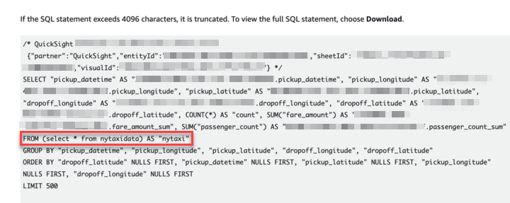
You will notice it loads the full dataset (select * from nytaxidata) as referenced in the screenshot below from RDS Performance Insight.

SQL from performance insight, unoptimized SQL inner query without where clause

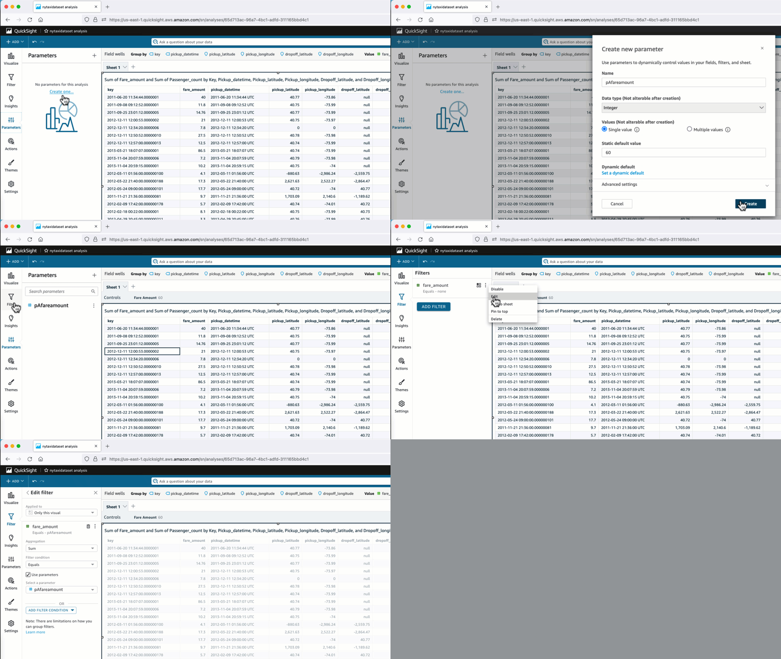
  1. Add an analysis parameter-based filter control to the QuickSight analysis. Change the value of this filter control (analysis parameter in this case).

creating analysis parameter with a control

The inner query over the dataset still uses custom SQL without using the filter in the WHERE clause. This filter control parameter is still part of the WHERE clause of the outer query, so the custom SQL fetches the complete result set as part of the inner query. This may not be the case if you use database tables as a dataset rather than a custom SQL query as a dataset. With a dataset based directly on tables, parameter values are passed to the database in the WHERE clause.

SQL from performance insight, unoptimized SQL inner query without where clause with analysis parameter

So how do we overcome the challenge of being able to include the parameter in the WHERE clause in custom SQL datasets? With dataset parameters!

Optimize your query with dataset parameters

Let’s look at a few scenarios where we can use dataset parameters to send more optimized queries to the database.

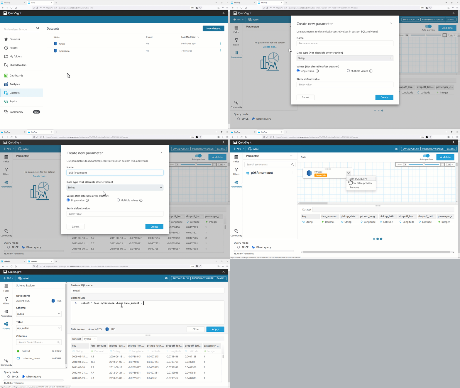
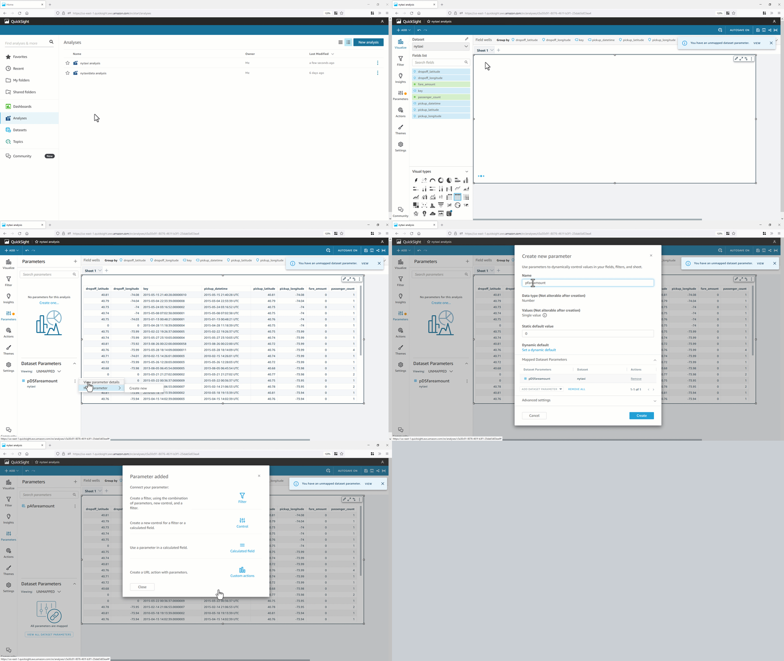
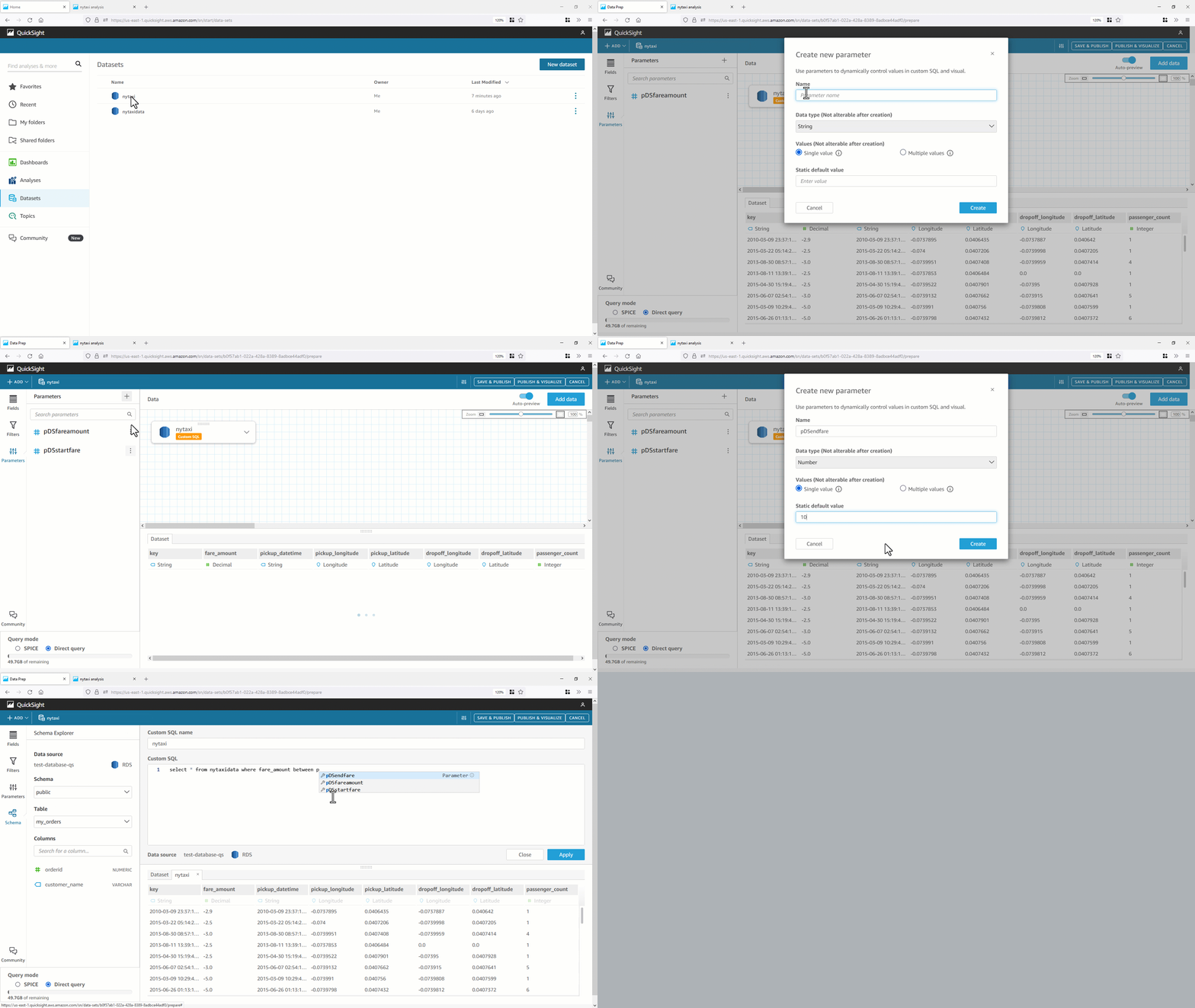
  1. Create a dataset parameter (for example, pDSfareamount) and add it to the WHERE clause with an equality predicate in the custom SQL.Observe if there is any change in the SQL query that was passed to the database.

creating dataset parameter

This time, you will see optimized SQL generated using the default parameter value in the WHERE clause of the inner query (select * from nytaxidata where fare_amount=0). This results in better query performance for direct query datasets.

optimized sql generated with dataset parameter

Map dataset parameters with analysis parameters

Dataset parameters can be mapped to analysis parameters and user-selected values can pass to the dataset parameters from the interactions on the dashboard at run time.

You can use a single analysis parameter and map it to multiple dataset parameters. The parent analysis parameter can now be linked with a filter control or an action, and can help you filter multiple datasets based on custom SQL.

In this section, we map a dataset parameter with an analysis parameter and bind it with a filter control at runtime.

  1. First, we create an analysis parameter and map it to a dataset parameter (we use the dataset parameter we created earlier).

mapping analysis parameter with a dataset parameter

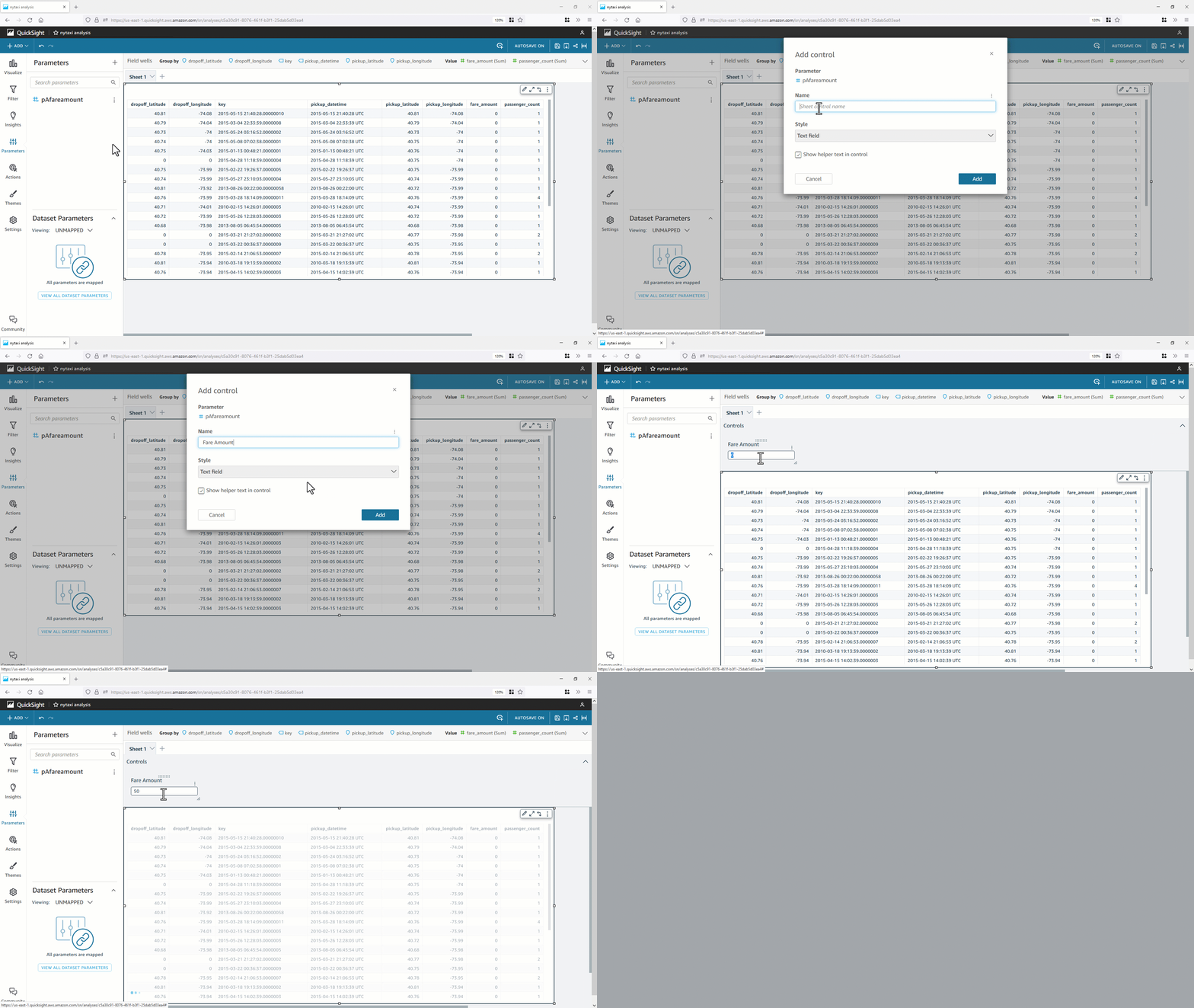
  1. Now the analysis parameter (for this example, pAfareamount) is created. You can create the control object Fare Amount to dynamically change the dataset parameter value from the analysis or dashboard using a parameter control. You can bind pAfareamount with a QuickSight filter to pass values to the dataset parameter dynamically. When you’re changing values in a parameter control, you will find optimized SQL on the backend database with the WHERE predicate in inner query generated.

chaing value of analysis parameter mapped to dataste parameter via filter control

Additional examples using dataset parameters

So far, we have used dataset parameters with an equality predicate.Let’s look at a few more scenarios using dataset parameters.

  1. The following screenshot demonstrates using a dataset parameter with a range predicate of custom SQL.

dataset parameter with non equality predicate

  1. The following example illustrates using two dataset parameters with a between operator.

two dataset parameters with between operator

  1. The following example shows using a dataset parameter within a calculation.

dataset parameter used in calculated field based on ifelse condition

  1. We can also use a dataset parameter with a scalar user-defined function (UDF). In the following example, we have a scalar function is_holiday(pickupdate), which takes a pickupdate as a parameter and returns a flag of 0 or 1 based on whether pickupdate is a public holiday.

dataset parameter used with scalar user defined function

  1. Additionally, we can use a dataset parameter to derive a calculated field. In the following example, we need to calculate the surcharge_amount dynamically based on a value specified at runtime and the number of passengers. We use a dataset parameter along with a case statement to calculate the desired surcharge_amount.

dataset paramter with calculated field case statement

  1. The final example illustrates how to move calculations using parameters in the analysis to the dataset for reusability.

porting dataset parameter from analysis to dataset

Dataset parameter limitations

The following are the known limitations (as of this writing) that you may encounter when working with dataset parameters in QuickSight:

  • Dataset parameters can’t be inserted into custom SQL of datasets stored in SPICE.
  • Dynamic defaults can only be configured on the analysis page of the analysis that is using the dataset. You can’t configure a dynamic default at the dataset level.
  • The Select all option is not supported on multi-value controls of analysis parameters that are mapped to dataset parameters (but there is a workaround that you can follow).
  • Cascading controls are not supported for dataset parameters.
  • Dataset parameters can only be used by dataset filters when the dataset is using a direct query.
  • When dashboard readers schedule emailed reports, selected controls don’t propagate to the dataset parameters that are included in the report that is attached to the email. Instead, the default values of the parameters are used.

Refer to Using dataset parameters in Amazon QuickSight for more information.

Conclusion

In this post, we showed you how to create QuickSight dataset parameters and map them to analysis parameters. Dataset parameters help improve your QuickSight dashboard performance for direct query custom SQL datasets by generating optimized SQL queries. We also showed a few examples of how to use dataset parameters in SQL range predicates, calculated fields, scalar UDFs, and case statements.

Dataset parameters enable dataset owners to centrally create and govern parameter-dependent calculated fields at the dataset level. Such calculated fields can be reused across multiple analyses, and cannot be tampered with by analysis authors.

We hope you will find dataset parameters in QuickSight useful. We have already seen how the feature is creatively used in a wide range of use cases. We recommend that you review your existing direct query custom SQL datasets in your QuickSight deployment to look for candidates for optimization, or take advantage of the other benefits of dataset parameters. For example, BI teams can benefit from dataset parameters by reusing the same dataset with different values in the parameter to analyze different slices of the same data, such as different regions, products, or customers by industry segments.

Are you considering migrating legacy reports to QuickSight? Dataset parameters can help enterprise BI developers reduce the migration effort of legacy reports that already have parameterized SQL queries in the legacy queries. These SQL queries can be passed along their parameters to QuickSight datasets via automations with the help of QuickSight APIs (and a few adjustments to the queries if the parameters are marked differently).

For more information on dataset parameters, refer to Using dataset parameters in Amazon QuickSight.


About the authors

Anwar Ali is a Specialist Solutions Architect for Amazon QuickSight. Anwar has over 18 years of experience implementing enterprise business intelligence (BI), data analytics and database solutions . He specializes in integration of BI solutions with business applications, helping customers in BI architecture design patterns and best practices.

Salim Khan is a Specialist Solutions Architect for Amazon QuickSight. Salim has over 16 years of experience implementing enterprise business intelligence (BI) solutions. Prior to AWS, Salim worked as a BI consultant catering to industry verticals like Automotive, Healthcare, Entertainment, Consumer, Publishing and Financial Services. He has delivered business intelligence, data warehousing, data integration and master data management solutions across enterprises.

Gil Raviv is a Principal Product Manager for Amazon QuickSight, AWS’ cloud-native, fully managed SaaS BI service. As a thought-leader in BI, Gil accelerated the growth of global BI practices at AWS and Avanade, and has guided Fortune 1000 enterprises in their Data & AI journey. As a passionate evangelist, author and blogger of low-code/no-code data prep and analytic tools, Gil was awarded 5 times as a Microsoft MVP (Most Valuable Professional).

Best practices for enabling business users to answer questions about data using natural language in Amazon QuickSight

Post Syndicated from Amy Laresch original https://aws.amazon.com/blogs/big-data/best-practices-for-enabling-business-users-to-answer-questions-about-data-using-natural-language-in-amazon-quicksight/

In this post, we explain how you can enable business users to ask and answer questions about data using their everyday business language by using the Amazon QuickSight natural language query function, Amazon QuickSight Q.

QuickSight is a unified BI service providing modern interactive dashboards, natural language querying, paginated reports, machine learning (ML) insights, and embedded analytics at scale. Powered by ML, Q uses natural language processing (NLP) to answer your business questions quickly. Q empowers any user in an organization to start asking questions using their own language. Q uses the same QuickSight datasets you use for your dashboards and reports so your data is governed and secured. Just as data is prepared visually using dashboards and reports, it can be readied for language-based interactions using a topic. Topics are collections of one or more datasets that represent a subject area that your business users can ask questions about. To learn how to create a topic, refer to Creating Amazon QuickSight Q topics.

With automated data preparation in QuickSight Q, the model will do a lot of the topic setup for you, but there is some context that is specific to your business that you need to provide. To learn more about the initial setup work that Q does behind the scenes, check out New – Announcing Automated Data Preparation for Amazon QuickSight Q.

Business users can access Q from the QuickSight console or embedded in your website or application. To learn how to embed the Q bar, refer to Embedding the Amazon QuickSight Q search bar for registered users or anonymous (unregistered) users. To see examples of embedded dashboards with Q, refer to the QuickSight DemoCentral.

Once you have a topic shared with your business users, they can ask their own questions and save questions to their pinboard as seen in GIF 1.

QuickSight authors can also add their Q visuals straight to an analysis to speed up dashboard creation, as seen in GIF 2.

This post assumes you’re familiar with building visual analytics in dashboards or reports, and shares new and different strategies needed to build natural language interfaces that are simple to use.

In this post, we discuss the following:

  • The importance of starting with a narrow and focused use case
  • Why and how to teach the system your unique business language
  • How to get success by providing support and having a feedback loop

If you don’t have Q enabled yet, refer to Getting started with Amazon QuickSight Q or watch the following video.

Follow along

In the following examples, we often refer to two out-of-the-box sample topics, Product Sales and Student Enrollment Statistics, so you can follow along as you go. We recommend creating the topics now before continuing with this post, because they take a few minutes to be ready.

Understand your users

Before we jump into solutions, let’s talk about when natural language query (NLQ) capabilities are right for your use case. NLQ is a fast way for a business user who is an expert in their business area to flexibly answer a large variety of questions from a scoped data domain. NLQ doesn’t replace the need for dashboards. Instead, when designed to augment a dashboard or reporting use case, NLQ helps business users get customized answers about specific details without asking a business analyst for help.

It’s critical to have a well-understood use case because language is inherently complex. There are many ways to refer to the same concept. For example, a university might refer to “classes” several ways, such as “courses,” “programs,” or “enrollments.” Language also has inherent ambiguity—“top students” might mean by highest GPA to one person and highest number of extracurriculars to another. By understanding the use case up front, you can uncover areas of potential ambiguity and build that knowledge directly into the topic.

For example, the AWS Analytics sales leadership team uses QuickSight and Q to track key metrics for their region as part of their monthly business review. When I worked with the sales leaders, I learned their preferred terminology and business language through our usability sessions. One observation I made was that they referred to the data field Sales Amortized Revenue as “adrr”. With these learnings, I could easily add this context to the topic using synonyms, which I cover in detail below. One of the sales leaders shared, “This will be awesome for next month when I write my MBR. What previously took a couple of hours, I can now do in a few minutes. Now I can spend more time working to deliver my customer’s outcomes.” If the sales leader asked a question about “adrr” but that connection was not included in their Q topic, then the leader would feel misunderstood and revert back to their original, but slower, ways of finding the answer. Check out more QuickSight use cases and success stories on the AWS Big Data Blog.

Start small

In this section, we share a few common challenges and considerations when getting started with Q.

Data can contain overlapping words

One pitfall to look out for is any fields with long strings, like survey write-in responses, product descriptions, and so on. This type of data introduces additional lexical complexity for readers to navigate. In other words, when an end-user asks a question, there is a higher chance that a word in one of the strings will overlap with other relevant fields, such as a survey write-in that mentions a product name in your Product field. Other non-descriptor fields can also contain overlaps. You can have two or more field names with lexical overlap, and the same across values, and even between fields and values. For example, let’s say you have a topic with a Product Order Status field with the values Open and Closed and a Customer Complaint Status field also with the values Open and Closed. To help avoid this overlap, consider alternate names that would be natural to your end-users to avoid the potential ambiguity. In our example, I’d keep the Product Order Status values and change the Customer Complaint Status to Resolved and Unresolved.

Avoid including aggregation names in your fields and values

Another common pitfall that introduces unnecessary ambiguity is including calculated fields for basic aggregations that Q can do on the fly. For example, business users might track average clickthrough rates for a website or month-to-date free to paid conversions. Although these types of calculations are necessary in a dashboard, with Q, these calculated fields are not needed. Q can aggregate metrics using natural language, like simply asking “year over year sales” or “top customers by sales” or “average product discount,” as you can see in Figure 1. Defining a field with the name YoY Sales adds an additional potential answer choice to your topic, leaving end-users to select between the pre-defined YoY Sales field, or using Q’s built-in YoY aggregation capability, whereas you may already know which of these choices is likely to bring them the best outcome. If you have complex business logic built into calculated fields, those are still relevant to include (and if you create the topic from your existing analysis, then Q will bring them over.)

Q answer showing MoM sales

Figure 1: Q visual showing MoM sales for EMEA

Start with a single use case

For this post, we recommend defining a use case as a well-defined set of questions that actual business users will ask. Q gives the ability to answer questions not already answered in dashboards and reports, so simply having a dashboard or a dataset doesn’t mean you necessarily have a Q-ready use case. These questions are the real words and phrases used by business users, like “how are my customers performing?” where the word “performing” might map in the data to “sales amortized revenue,” but a business user might not ask questions using the precise data names.

Start with a single use case and the minimum number of fields to meet it. Then incrementally layer in more as needed. It’s better to introduce a topic with, for example, 10 fields and a 100% success rate of answering questions as expected vs. starting with 30 fields and a 70% success rate to help users feel confident.

To help you start small, Q enables you to create your topic in one click from your existing analysis (Figure 2).

Enable a Q topic from a QuickSight analysis

Figure 2: Enable a Q topic from a QuickSight analysis

Q will scan the underlying metadata in your analysis and automatically select high-value columns based on how they are used in the analysis. You’ll also get all your existing calculated fields ported over to the new topic so you don’t have to re-create them.

Add lexical context

Q knows English well. It understands a variety of phrases and different forms of the same word. What it doesn’t know is the unique terms from your business, and only you can teach it.

There are some key ways to provide Q this context, including adding synonyms, semantic types, default aggregations, primary date, named filters, and named entities. If you created your Q topic as described in the previous section, you will be a few steps ahead, but it’s always good to check the model’s work.

Add synonyms

In a dashboard, authors use visual titles, text boxes, and filter names to help business users navigate and find their answers. With NLQ, language is the interface. NLQ empowers business users to ask their questions in their own words. The author needs to make those business lexicon connections for Q using synonyms. Your business users might refer to revenue as “gross sales,” “amortized revenue,” or any number of terms specific to your business. From the topic authoring page, you can add relevant terms (Figure 3).

Add Q synonyms

Figure 3: Adding relevant synonyms

If your business users refer to the data values in multiple ways, you can use value synonyms to create those connections for Q (Figure 4). For example, in the Student Enrollment topic, let’s say your business users sometimes use First Years to map to Freshmen and so on for each classification type. If you don’t have that data directly in your dataset, you can create those mappings using value synonyms (Figure 5).

Configure Q value synonyms

Figure 4: Configure field value synonyms

Add Q value synonyms

Figure 5: Example value synonyms for Student Enrollment topic

Check semantic types

When you create a topic using automatic data prep, Q will automatically select relevant semantic types that it can detect. Q uses semantic types to understand which specific fields to use to answer vague question like who, where, when, and how many. For example, in the student enrollment statistics example, Q already set Home of Origin as Location so if someone asks “where,” Q knows to use this field (Figure 6). Another example is adding Person for the Student Name and Professor fields so Q knows what fields to use when your business users ask for “who.”

Home of origin semantic type

Figure 6: Semantic Type set to “Location”

Another important semantic type is the Identifier. This tells Q what to count when your business users ask questions like “How many were enrolled in biology in 2021?” (Figure 7). In this example, Student ID is set as the Identifier.

Q answer showing a KPI of 3

Figure 7: Q visual showing a “how many” question

Here is a list of semantic types that map to implicit question phrases:

  • Location: Where?
  • Person or Organization: Who?
    • If there are no person or organization fields, then Q will use the identifier
  • Identifier: How many? What is the number of?
  • Duration: How long?
  • Date Part: When?
  • Age: How old?
  • Distance: How far?

Semantic types also help the model in several other ways, including mapping terms like “most expensive” or “cheapest” to Currency. There is not always a relevant semantic type, so it’s okay to leave those empty.

Set default aggregations

Q will always aggregate measure values a business user asks for, so it’s important to use measures that retain their meaning when brought together with other values. As of this writing, Q works best with underlying data that is summative, for example, a currency value or a count. Examples of metrics that are not summative are percentages, percentiles, and medians. Measures of this type can produce misleading or statistically inaccurate results when added with one another. Q can be used to produce averages, percentiles, and medians by end-users without first performing those calculations in underlying data.

Help Q understand the business logic behind your data by setting default aggregations. For example, in the Student Enrollment topic, we have student test scores for every course, which should be averaged and not summed, because it’s a percentage. Therefore, we set Average as the default and set Sum as a not allowed aggregation type (Figure 8).

Percentage semantic type

Figure 8: Setting “Sum” as a “Not allowed aggregation” for a percentage data field

To ensure end-users get a correct count, consider whether the default aggregation type for each dimensional field should be Distinct Count or Count and set accordingly. For example, if we wanted to ask “how many courses do we offer,” we would want to set Courses to Distinct Count because the underlying data contains multiple records for the same course to track each student enrolled.

If we have a count, we get over 6,000 courses, which is a count of all rows that have data in the Courses field, covering every student in the dataset (Figure 9).

Q KPI showing 6,277

Figure 9: Q visual showing a count of courses

If we set the default aggregation to Distinct Count, we get the count of unique course names, which is more likely to be what the end-user expects (Figure 10).

Q KPI showing 15

Figure 10: Q visual showing the unique count of courses

Review the primary date field

Q will automatically select a primary date field for answering time related questions like “when” or “yoy”. If your data includes more than one date field, you may want to choose a different date than Q’s default choice. End-users can also ask about additional date fields by explicitly naming them (Figure 12). You can always specify a different date if you’d like. To review or change the primary date, go to the topic page, navigate to the Data section, and choose the Datasets tab. Expand the dataset and review the value for Default date (Figure 11).

Reviewing the Q default date

Figure 11: Reviewing the default date

You can change the date as needed.

Changing the date field

Figure 12: Asking about non-default dates

Add named filters

In a dashboard, filters are critical to allow users to focus in on their area of interest. With Q, traditional filters aren’t required because users can automatically ask to filter any field values included in the Q topic. For example, you could ask “What were sales last week for Acme Inc. for returning shoppers?” Instead of building the filters in a dashboard (date, customer name, and returning vs. new customer), Q does the filtering on the fly to instantly provide the answer.

With Q, a filter is a specific word or phrase your business users will use to instruct Q to filter returned results. For example, you have student test scores but you want a way for your users to ask about failing test scores. You can set up a filter for “Failing” defined as test scores less than 70% (Figure 13).

Q filter configuration

Figure 13: Filter configuration example using a measure

Additionally, maybe you have a field for Student Classification, which includes Freshmen, Sophomore, Junior, Senior, and Graduate, and you want to let users ask about “undergrads” vs. “graduates” (Figure 14). You can make a filter that includes the relevant values.

Q undergrad named filter example

Figure 14: Filter configuration example using a dimension

Add named entities

Named entities are a way to get Q to return a set of fields as a table visual when a user asks for a specific word or phrase. If someone wanted to know “sales for retail december” and they get a KPI saying $6,169 without any extra context, it is hard to understand all data this number includes (Figure 15).

Q KPI showing $6,169

Figure 15: A Q visual showing “sales for retail december”

By presenting the KPI in a table view with other relevant dimensions, the data includes additional context making it easier to understand meaning (Figure 16).

Q named entity as a table visual

Figure 16: A Q visual showing “sales details for retail december”

By building these table views, you can happily surprise your business users by anticipating the information they want to see without having to explicitly ask for each piece of data. The best part is your business users can easily filter the table using language to answer their own data questions. For example, in the Student Enrollment topic, we created a Student information named entity with some important student details like their name, major, email, and test scores per course.

Q named entity for student information

Figure 17: Named entity example

If a university administrator wanted to reach out to students who are failing biology, they can simply ask for “student information for failing biology majors.” In one step, they get a filtered list that already includes their emails and test scores so they can reach out (Figure 18).

Q named entity filtered down for failing biology students

Figure 18: Filtering a named entity

If the university administrator wanted to also see the phone numbers of the students to send texts offering free tutoring, they could simply ask Q “Student information for failing biology majors with phone numbers.” Now, Mobile is added as the first column (Figure 19).

Q named entity adding phone number

Figure 19: Adding a column to a named entity

Entities can also be referenced using synonyms in order to capture all the ways your business users might refer to this group of data. In our example, we could also add “student contact info” and “academic details” based on the common terminology the university admins use.

Besides looking for patterns in the data fields, ask yourself about what your business users care about. For example, let’s assume we have data for our HR specialists, and we know they care about job postings, candidates, and recruiters. Each author might think of the groups slightly differently, but as long as it’s rooted in your business jobs to be done, then your groupings are providing value. With those three groups in mind, we can sort all the data into one of those buckets. For this use case, our Candidate bucket is pretty large, with about 20 fields. We can scan the list and notice that we track information for rejected and accepted candidates, so we start splitting the metrics into two groups: Successful Candidates and Rejected Candidates. Now information like Offer Letter Date, Accept Date, and Final Salary are all in the Successful Candidate group, and related fields about Rejected Candidates are clearly grouped together.

If you’re curious about strategies for how to create entities, check out card sorting techniques.

In the Product Sales sample topic, after scanning the data, we would start with Sales, Product, and Customer as three key groupings of information to analyze. Try out the exercise on your own data and feel free to ask any questions on the QuickSight Community. To learn how to create named entities, refer to Adding named entities to a topic dataset.

Drive NLQ adoption

After you have refined your topic, tested it out with some readers, and made it available for a larger audience, it’s important to follow two strategies to drive adoption.

First, provide your business users with support. Support might look like a short tutorial video or newsletter announcement. Consider keeping an open channel like a Slack or Teams chat where active users can post questions or enhancements.

Here at Amazon, the Prime team has a dedicated Product Manager (PM) for their embedded Q application that they call PrimeQ. The PM hosts regular demo and training sessions where the Prime team can ask them any questions and get ideas about what types of answers they can get. The PM also sends out a monthly newsletter to announce the availability of new data and topics along with sample questions, FAQs, and quotes from Prime team members who get value out of Q. The PM also has an active Slack channel where every single question gets answered within 24 hours, either by the PM or a data engineer on the Prime team.

Pro tip: Make sure your business users know who they can reach out to if they get stuck. Avoid the black box of “reach out to your author” so readers feel confident their questions will be answered by a known person. For embedded applications, be sure to build an easy way to get support.

Second, maintain a healthy feedback loop. Look at the usage data directly in the product and schedule 1-on-1 sessions with your readers. Use the usage data to track adoption and identify readers who are asking unanswerable questions (Figure 20). Engage with both your successful and struggling readers to learn how to continue to iterate and improve the experience. Talking to business users is especially important to uncover the implicit ambiguity of language.

Another example here at Amazon, after first launching the Revenue Insights topic for the AWS Analytics sales team, a QuickSight Solution Architect (SA) and myself checked the usage tab on a daily basis to track unanswerable questions and directly reach out to the sales team member to let them know how to adjust their question or that we made a change so their question would now work. For example, we initially had a field turned off for Market Segment and noticed a question from a sales leader asking about sales by segment. We turned the field on and let him know those questions would now work. The SA and I have a Slack channel with other stakeholders so we can troubleshoot asynchronously with ease. Now that the topic has been available for several months, we check the usage tab on a weekly basis.

Q user activity tab

Figure 20: User Activity tab in Q

Conclusion

In this post, we discussed how language is inherently complex and what context you need to provide Q to teach the system about your unique business language. Q’s automated data prep will get you started, but you need to add the context that is specific to your business user’s language. As we mentioned at the start of the post, consider the following:

  • Start with a narrow and focused use case
  • Teach the system your unique business language
  • Get success by providing support and having a feedback loop

Follow this post to enable your business users to answer questions of data using natural language in QuickSight.

Ready to get started with Q? Watch our quick tutorial on enabling QuickSight Q.

Want some tutorial videos to share with your team? Check out the following:

To see how Q can answer the “Why” behind data changes and forecast future business performance, refer to New analytical questions available in Amazon QuickSight Q: “Why” and “Forecast”.


About the Author

Amy Laresch is a product manager for Amazon QuickSight Q. She is passionate about analytics and is focused on delivering the best experience for every QuickSight Q reader. Check out her videos on the @AmazonQuickSight YouTube channel for best practices and to see what’s new for QuickSight Q.

Deploying an automated Amazon CloudWatch dashboard for AWS Outposts using AWS CDK

Post Syndicated from Sheila Busser original https://aws.amazon.com/blogs/compute/deploying-an-automated-amazon-cloudwatch-dashboard-for-aws-outposts-using-aws-cdk/

This post is written by Enrico Liguori, Networking Solutions Architect, Hybrid Cloud and Sumeeth Siriyur, Sr. Hybrid Cloud Solutions Architect.

AWS Outposts is a fully managed service that brings the same AWS infrastructure, services, APIs, and tools to virtually any data center, colocation space, manufacturing floor, or on-premises facility where it might be needed. With Outposts, you can run some AWS services on-premises and connect to a broad range of services available in the local AWS Region. Outposts supports workloads requiring low latency, local data processing, data residency, and application migration.

Outposts capacity is driven as per your compute and storage requirements to run workloads. You can monitor Outposts resources using metrics gathered by Amazon CloudWatch. Using these metrics, you can effectively monitor and manage the Outposts resources as they would in the Region, levereging cloud native tools such as CloudWatch dashboards. Check the Monitoring best practices for AWS Outposts blog post to dive deep into the available monitoring options for Outposts.

CloudWatch dashboards are customizable home pages in the CloudWatch console that can be used to monitor resources running on Outposts in a single view. For example, you can monitor in a single pane the number Amazon EC2 instances used per EC2 instance type, the available capacity of Amazon EBS volumes and Amazon S3 buckets, and the operational status of the service link of Outposts.

As a you start deploying additional Outposts resources as a part of their capacity expansion, they must all be integrated and visualized within CloudWatch in an automated way. Traditionally CloudWatch dashboards are built manually and may be time consuming to tune. This post provides also an overview of building CloudWatch dashboards in an automated way using AWS Cloud Development Kit (AWS CDK).

Overview

CloudWatch metrics available to monitor Outposts resources and capacity

CloudWatch metrics for Outposts are available to customers in all public AWS Regions and AWS GovCloud (US) at no additional cost. We can classify the available metrics in two main categories:

To identify the metrics published under the service specific namespaces, we can leverage metadata in the form of tags. A tag is a label that you assign to an AWS resource and consists of a key and an optional value. For the purpose of the monitoring strategy described in this post, we use a tag that contains the OutpostID of the Outpost where the resource is deployed. In this way, we can easily filter the CloudWatch metrics that we would like to show in our dashboard.

To enforce the assignment of tags to our resources we can implement a tagging strategy using AWS tag Policies and Service Control Policies (SCPs).

The following sections describe two different methods to build a CloudWatch dashboard that includes the different types of metrics described so far. In both cases, we see how particularly useful the presence of tags is to identify the service-specific metrics.

Manual approach to building a CloudWatch dashboard for Outposts

This section describes a manual (i.e., non-automated) approach to building a dashboard that could summarize both the capacity utilization metrics and the service specific metrics for your resources running on Outposts.

The benefit of this approach is that we can implement a fully operational dashboard directly from the CloudWatch console. However, it will simultaneously require more effort to properly tune the dashboard to satisfy your monitoring requirements.

You can start creating the dashboard opening the CloudWatch console and following the steps listed in the public documentation.

To display a metric under AWS/Outposts namespace we can choose any of the widgets available. Based on the nature of the data, we can choose different types of Widgets such as Number, Line, Gauge, Explorer, or you can even build your own custom widget.

Together with the Widget type, we must select Outposts namespace in the metric graph dialog box and then navigate to the specific metric of interest.

In case we are creating the dashboard in a different account than the Outposts owner, we must select the right account in the View data drop-down menu to see the Outposts metric in which we are interested.

View data drop-down menu

After selecting one or more metrics we can select Create widget button.

For the service specific metrics, we recommend using the explorer widget. In this way, we can utilize the tagging strategy described earlier to automatically identify the metrics belonging to the resources running on Outposts. Check the documentation page for a step-by-step guide for creating an explorer widget based on tags.

Automated outpost dashboard

After we’ve seen how to build a dashboard manually from the console, in this secton we describe an automated approach to deploy a dashboard for Outposts through AWS CDK.

AWS CDK is an open source software development framework to model and provision your cloud application resources using familiar programming languages, including TypeScript, JavaScript, Python, C#, and Java. For the solution in this post, we use Python.

Architecture overview

The AWS CDK stack described in this post, assumes that the resources running on Outposts (EC2 instances, S3 buckets, Application Load Balancers (ALBs), and RDS instances) are tagged using the tagging strategy described earlier.

Specifying a tag name and a tag value in a configuration file automatically discovers the resources with that tag and adds the related metrics to the CloudWatch dashboard.

Together with the service specific metrics, it creates a series of widgets that we can use to monitor the capacity available and utilized in each Outpost that belongs to the account where the script is running.

The workflow is made of the following phases:

  1. The AWS CDK stack creates an AWS CodeCommit repository and uploads its own code into it. The code contains a series of modules, one for each section of the CloudWatch dashboard. A section of the dashboard contains one or more widgets showing the metrics of a specific service.
  2. To maintain the CloudWatch dashboard always up-to-date with the resources matching the tag, it creates a pipeline in AWS CodePipeline that can dynamically create and or update the dashboard. The pipeline runs the code in the CodeCommit repository and is made of two stages. In the first one, the build stage, it builds the dependencies needed by the AWS CDK stack. In the second stage, the Deploy stage, it loads and runs the modules used to build the dashboard.
  3. Each module contains the code to automatically discover the tagged resources of a specific service. This discovery phase uses standard AWS APIs called through the Python SDK Boto3.
  4. Based on the results of the discovery phase, AWS CDK produces an AWS CloudFormation template containing the definition of the CloudWatch dashboard sections. The template is submitted to CloudFormation.
  5. CloudFormation creates or, if already defined, updates the CloudWatch dashboard.
  6. Together with the dashboard, the AWS CDK script also contains the definition of a CloudWatch Event that, once deployed, triggers the pipeline each time a resource tagged with the specified tag is created or destroyed.

Prerequisites

To implement the solution presented in this post, you must configure:

  1. git as distributed version control system.
  2. In case it is the first time that you’re using AWS CDK in this account and region, you must:

a. Install the AWS CDK, and its prerequisites, following these instructions.

b. Go through the AWS CDK bootstrapping process. This is required only for the first time that we use AWS CDK in a specific AWS environment (an AWS environment is a combination of an AWS account and Region).

How to install

Step 1: Clone the AWS CDK code hosted on GitHub with:

$ git clone https://github.com/aws-samples/automated-cloudwatch-dashboard.git

Step 2: enter the directory using the following:

$ cd  automated-cloudwatch-dashboard/

Step 3: Install the needed Python dependencies with:

$ pip install -r requirements.txt

Step 4: Modify the configuration file

Before deploying the stack, we must modify the configuration file to specify the tag we use for identifying our resources running on Outposts. Open the file with the name config.yaml with your preferred text editor and specify:

      • A name for the dashboard. The default name used is Automated-CloudWatch-Dashboard.
      • Replace <tag_name> placeholder following the tag_name variable with the tag name used to tag the resources that you want to include in the dashboard.
      • Replace <tag_value> placeholder under tag_values variable with the tag value that you used.

Here is an example config.yaml configuration file:

dashboard_name: Automated-CloudWatch-Dahsboard
tag_name: OutpostID
tag_values:
  - op-1234567890abcdefg 

Stack deployment

We can deploy the stack with the following:

$ cdk deploy

At the end of the deployment process, the pipeline that creates the dashboard is provisioned. You can now go to your CloudWatch console to view it.

Automated Outposts dashboard overview

Now that we have built our dashboard, let’s review each section:

  1. Outpost capacity

Outpost Capacity diagram

The AWS CDK stacks define a capacity section for each Outpost available to the AWS account where the script runs.

In this section, we find four widgets showing metrics published under the AWS/Outpost namespace. The first widget shows for each EC2 instance type available on the Outposts the number of instances utilized and available for that instance type. In the second row, we can visualize the available capacity for the Amazon EBS volumes and for the S3 buckets. The last widget shows the operational status of the service link of Outposts.

2. EC2 instances

CPU, Network, and Disk Utilization for an EC2 instance diagram

In this section of the dashboard, we find the metrics showing the CPU, Network, and Disk Utilization for an EC2 instance. It has defined a section of this type for each EC2 instance with a tag assigned matching the name and the value specified in the configuration file of the script.

3. Application Load Balancer

The ALB section aggregates metrics showing the operational status of a load balancer hosted on Outposts

The ALB section aggregates metrics showing the operational status of a load balancer hosted on Outposts. A section of this type is defined for each ALB with an assigned tag matching the one specified in the configuration file.

4. S3 buckets

The S3 buckets section diagram

The S3 buckets section is defined only once and aggregates the utilization metrics for all S3 buckets with an assigned tag.

5. AutoScaling group

The AutoScaling group section diagram

The AutoScaling group section can be used to monitor the number of instances in service in a specific AS group with a tag assigned. This section is defined once and can aggregate the metrics for multiple AutoScaling groups.

Clean up

To terminate the resources that we created in this post, run the following:

$ cdk destroy

Then, go to the Cloudformation console and delete the stack with the name “Deploy-AutomatedCloudWatchDashboard”.

Conclusion

In conclusion, this post demonstrates a manual way of creating CloudWatch Metrics dashboard using the CloudWatch console and an automated way using AWS CDK. The automated approach is also scalable by automatically discovering any new resources added to the existing Outposts in the your environment without any changes to the code.

Best practices for running production workloads using Amazon MSK tiered storage

Post Syndicated from Nagarjuna Koduru original https://aws.amazon.com/blogs/big-data/best-practices-for-running-production-workloads-using-amazon-msk-tiered-storage/

In the second post of the series, we discussed some core concepts of the Amazon Managed Streaming for Apache Kafka (Amazon MSK) tiered storage feature and explained how read and write operations work in a tiered storage enabled cluster.

This post focuses on how to properly size your MSK tiered storage cluster, which metrics to monitor, and the best practices to consider when running a production workload.

Sizing a tiered storage cluster

Sizing and capacity planning are critical aspects of designing and operating a distributed system. It involves estimating the resources required to handle the expected workload and ensure the system can scale and perform efficiently. In the context of a distributed system like Kafka, sizing involves determining the number of brokers, the number of partitions, and the amount of storage and memory required for each broker. Capacity planning involves estimating the expected workload, including the number of producers, consumers, and the throughput requirements.

Let’s assume a scenario where the producers are evenly balancing the load between brokers, brokers host the same number of partitions, there are enough partitions to ingest the throughput, and consumers consume directly from the tip of the stream. The brokers are receiving the same load and doing the same work. We therefore just focus on Broker1 in the following diagram of a data flow within a cluster.

Theoretical sustained throughput with tiered storage

We derive the following formula for the theoretical sustained throughput limit tcluster given the infrastructure characteristics of a specific cluster with tiered storage enabled on all topics:

max(tcluster) <= min {

max(tstorage) * #brokers/(r + 1 + #non_tip_local_consumer_groups),
max(tNetworkAttachedStorage) * #brokers/(r + 1 + #non_tip_local_consumer_groups),
max(tEC2network) * #brokers/(#tip_consumer_groups + r + #remote_consumer_groups)

}

This formula contains the following values:

  • tCluster – Total ingress produce throughput sent to the cluster
  • tStorage – Storage volume throughput supported
  • tNetworkAttachedStorage – Network attached storage to the Amazon Elastic Compute Cloud (Amazon EC2) instance network throughput
  • tEC2network – EC2 instance network bandwidth
  • non_tip_local_consumer_groups – Number of consumer groups reading from network attached storage at ingress rate
  • tip_consumer_groups – Number of consumer groups reading from page cache at ingress rate
  • remote_consumer_groups – Number of consumer groups reading from remote tier at ingress rate
  • r – Replication factor of the Kafka topic

Note that in the first post , we didn’t differentiate between different types of consumer groups. With tiered storage, some consumer groups might be consuming from remote. These remote consumers might ultimately catch up and start reading from local storage and finally catch up to the tip. Therefore, we model these three different consumer groups in the equation to account for their impact on infrastructure usage. In the following sections, we provide derivations of this equation.

Derivation of throughput limit from network attached storage bottleneck

Because Amazon MSK uses network attached storage for local storage, both network attached storage throughput and bandwidth should be accounted for. Total throughput bandwidth requirement is a combination of ingress and egress from the network attached storage backend. The ingress throughput of the storage backend depends on the data that producers are sending directly to the broker plus the replication traffic the broker is receiving from its peers. With tiered storage, Amazon MSK also uses network attached storage to read and upload rolled segments to the remote tier. This doesn’t come from the page cache and needs to be accounted for at the rate of ingress. Any non-tip consumers at ingress rate also consume network attached storage throughput and are accounted for in the equation. Therefore, max throughput is bounded by network attached storage based on the following equation:

max(tcluster) <= min {

max(tstorage) * #brokers/(r + 1 + #non_tip_local_consumer_groups),
max(tNetworkAttachedStorage) * #brokers/(r + 1 + #non_tip_local_consumer_groups)

}

Derivation of throughput limit from EC2 network bottleneck

Unlike network attached storage, the network is full duplex, meaning that if the EC2 instance supports X MB/s network, it supports X MB/s in and X MB/s out. The network throughput requirement depends on the data that producers are sending directly to the broker plus the replication traffic the broker is receiving from its peers. It also includes the replication traffic out and consumers traffic out from this broker. With tiered storage, we need to reserve additional ingress rate for uploads to the remote tier and support reads from the remote tier for consumer groups reading from remote offset. Both of these add to the network out requirements, which is bounded by the following equation:

max(tcluster) <= min {

max(tEC2network) * #brokers/(#tip_consumer_groups + r + #remote_consumer_groups)

}

Combining the second and third equations provides the first formula, which determines the max throughput bound based on broker infrastructure limits.

How to apply this formula to size your cluster

With this formula, you can calculate the upper bound for throughput you can achieve for your workloads. In practice, the workloads may be bottlenecked by other broker resources like CPU, memory, and disk, so it’s important to do load tests. To simplify your sizing estimate, you can use the MSK Sizing and Pricing spreadsheet (for more information, refer to Best Practices).

Let’s consider a workload where your ingress and egress rates are 20MB/s, with a replication factor of 3, and you want to retain data in your Kafka cluster for 7 days. This workload requires 6x m5.large brokers, with 34.6 TB local storage, which will cost $6,034.00 monthly (estimated). But if you use tiered storage for the same workload with local retention of 4 hours and overall data retention of 7 days, it requires 3x m5.large brokers, with 0.8 TB local storage and 12 TB of tiered storage, which will cost $1,958.00 monthly(estimated). If you want to read all the historic data one time, it will cost $17.00 ($0.0015 per GB retrieval cost). In this example with tiered storage, you save around 67.6% of your overall cost.

We recommend planning for Availability Zone redundancy in production workloads considering the broker safety factor in the calculation, which is 1 in this example. We also recommend running performance tests to ensure CPU is less than 70% on your brokers at the target throughput derived based on this formula or Excel calculation. In addition, you should also use the per-broker partition limit in your calculation to account for other bottlenecks based on the partition count.

The following figure shows an example of Amazon MSK sizing.

Monitoring and continuous optimization for a tiered storage enabled cluster

In previous sections, we emphasized the importance of determining the correct initial cluster size. However, it’s essential to recognize that sizing efforts shouldn’t cease after the initial setup. Continual monitoring and evaluation of your workload are necessary to ensure that the broker size remains appropriate. Amazon MSK offers metric monitoring and alarm capabilities to provide visibility into cluster performance. In the post Best practices for right-sizing your Apache Kafka clusters to optimize performance and cost, we discussed key metrics to focus on. In this post, we delve deeper into additional metrics related to tiered storage and other optimization considerations for a tiered storage enabled cluster:

  • TotalTierBytesLag indicates the total number of bytes of the data that is eligible for tiering on the broker and hasn’t been transferred to the tiered storage yet. This metric shows the efficiency of upstream data transfer. As the lag increases, the amount of data that hasn’t yet persisted in the tiered storage increases. The impact is the network attached storage disk may fill up, which you should monitor. You should also monitor this metric and generate an alarm if the lag is continuously growing and you see increased network attached storage usage. If the tiering lag is too high, you can reduce ingress traffic to allow the tiered storage to catch up.
  • Although tiered storage provides on-demand, virtually unlimited storage capacity without provisioning any additional resources, you should still do proper capacity planning for your local storage, configure alerts for KafkaDataLogsDiskUsed metrics, and have a buffer on network attached storage capacity planning. Monitor this metric and generate an alarm if the metric reaches or exceeds 60%. For a tiered storage enabled topic, configure local retention accordingly to reduce network attached storage usage.
  • The theoretical max ingress we can achieve on an MSK cluster with tiered storage is 20–25% lower than a non-tiered storage enabled cluster due to additional network attached storage bandwidth required to transparently move data from the local to the remote tier. Plan for the capacity (brokers, storage, gp2 vs. gp3) using the formula we discussed to derive max ingress for your cluster based on the number of consumer groups and load test your workloads to identify the sustained throughput limit. Exercising excess ingress to the cluster or egress from the remote tier above the planned capacity can impact your tip produce or consume traffic.
  • The gp3 volume type offers SSD-performance at a 20% lower cost per GB than gp2 volumes. Furthermore, by decoupling storage performance from capacity, you can easily provision higher IOPS and throughput without the need to provision additional block storage capacity. Therefore, we recommend using gp3 for a tiered storage enabled cluster by specifying provisioned throughput for larger instance types.
  • If you specified a custom cluster configuration, check the num.replica.fetchers, num.io.threads, and num.network.threads configuration parameters on your cluster. We recommend leaving it as the default Amazon MSK configuration unless you have specific use case.

This is only the most relevant guidance related to tiered storage. For further guidance on monitoring and best practices of your cluster, refer to Best practices.

Conclusion

You should now have a solid understanding of how Amazon MSK tiered storage works and the best practices to consider for your production workload when utilizing this cost-effective storage tier. With tiered storage, we remove the compute and storage coupling, which can benefit workloads that need larger disk capacity and are underutilizing compute just to provision storage.

We are eager to learn about your current approach in building real-time data streaming applications. If you’re starting your journey with Amazon MSK tiered storage, we suggest following the comprehensive Getting Started guide available in Tiered storage. This guide provides detailed instructions and practical steps to help you gain hands-on experience and effectively take advantage of the benefits of tiered storage for your streaming applications.

If you have any questions or feedback, please leave them in the comments section.


About the authors

Nagarjuna Koduru is a Principal Engineer in AWS, currently working for AWS Managed Streaming For Kafka (MSK). He led the teams that built MSK Serverless and MSK Tiered storage products. He previously led the team in Amazon JustWalkOut (JWO) that is responsible for realtime tracking of shopper locations in the store. He played pivotal role in scaling the stateful stream processing infrastructure to support larger store formats and reducing the overall cost of the system. He has keen interest in stream processing, messaging and distributed storage infrastructure.

Masudur Rahaman Sayem is a Streaming Data Architect at AWS. He works with AWS customers globally to design and build data streaming architectures to solve real-world business problems. He specializes in optimizing solutions that use streaming data services and NoSQL. Sayem is very passionate about distributed computing.

AWS Security Hub launches a new capability for automating actions to update findings

Post Syndicated from Stuart Gregg original https://aws.amazon.com/blogs/security/aws-security-hub-launches-a-new-capability-for-automating-actions-to-update-findings/

If you’ve had discussions with a security organization recently, there’s a high probability that the word automation has come up. As organizations scale and consume the benefits the cloud has to offer, it’s important to factor in and understand how the additional cloud footprint will affect operations. Automation is a key enabler for efficient operations and can help drive down the number of repetitive tasks that the operational teams have to perform.

Alert fatigue is caused when humans work on the same repetitive tasks day in and day out and also have a large volume of alerts that need to be addressed. The repetitive nature of these tasks can cause analysts to become numb to the importance of the task or make errors due to manual processing. This can lead to misclassification of security alerts or higher-severity alerts being overlooked due to investigation times. Automation is key here to reduce the number of repetitive tasks and give analysts time to focus on other areas of importance.

In this blog post, we’ll walk you through new capabilities within AWS Security Hub that you can use to take automated actions to update findings. We’ll show you some example scenarios that use this capability and set you up with the knowledge you need to get started with creating automation rules.

Automation rules in Security Hub

AWS Security Hub is available globally and is designed to give you a comprehensive view of your security posture across your AWS accounts. With Security Hub, you have a single place that aggregates, organizes, and prioritizes your security alerts, or findings, from multiple AWS services, including Amazon GuardDuty, Amazon Inspector, Amazon Macie, AWS Firewall Manager, AWS Systems Manager Patch Manager, AWS Config, AWS Health, and AWS Identity and Access Management (IAM) Access Analyzer, as well as from over 65 AWS Partner Network (APN) solutions.

Previously, Security Hub could take automated actions on findings, but this involved going to the Amazon EventBridge console or API, creating an EventBridge rule, and then building an AWS Lambda function, an AWS Systems Manager Automation runbook, or an AWS Step Functions step as the target of that rule. If you wanted to set up these automated actions in the administrator account and home AWS Region and run them in member accounts and in linked Regions, you would also need to deploy the correct IAM permissions to enable the actions to run across accounts and Regions. After setting up the automation flow, you would need to maintain the EventBridge rule, Lambda function, and IAM roles. Such maintenance could include upgrading the Lambda versions, verifying operational efficiency, and checking that everything is running as expected.

With Security Hub, you can now use rules to automatically update various fields in findings that match defined criteria. This allows you to automatically suppress findings, update findings’ severities according to organizational policies, change findings’ workflow status, and add notes. As findings are ingested, automation rules look for findings that meet defined criteria and update the specified fields in findings that meet the criteria. For example, a user can create a rule that automatically sets the finding’s severity to “Critical” if the finding account ID is of a known business-critical account. A user could also automatically suppress findings for a specific control in an account where the finding represents an accepted risk.

With automation rules, Security Hub provides you a simplified way to build automations directly from the Security Hub console and API. This reduces repetitive work for cloud security and DevOps engineers and can reduce the mean time to response.

Use cases

In this section, we’ve put together some examples of how Security Hub automation rules can help you. There’s a lot of flexibility in how you can use the rules, and we expect there will be many variations that your organization will use when contextual information about security risk has been added.

Scenario 1: Elevate finding severity for specific controls based on account IDs

Security Hub offers protection by using hundreds of security controls that create findings that have a severity associated with them. Sometimes, you might want to elevate that severity according to your organizational policies or according to the context of the finding, such as the account it relates to. With automation rules, you can now automatically elevate the severity for specific controls when they are in a specific account.

For example, the AWS Foundational Security Best Practices control GuardDuty.1 has a “High” severity by default. But you might consider such a finding to have “Critical” severity if it occurs in one of your top production accounts. To change the severity automatically, you can choose GeneratorId as a criteria and check that it’s equal to aws-foundational-security-best-practices/v/1.0.0/GuardDuty.1, and also add AwsAccountId as a criteria and check that it’s equal to YOUR_ACCOUNT_IDs. Then, add an action to update the severity to “Critical,” and add a note to the person who will look at the finding that reads “Urgent — look into these production accounts.”

You can set up this automation rule through the AWS CLI, the console, the Security Hub API, or the AWS SDK for Python (Boto3), as follows.

To set up the automation rule for Scenario 1 (AWS CLI)

  • In the AWS CLI, run the following command to create a new automation rule with a specific Amazon Resource Name (ARN). Note the different modifiable parameters:
    • Rule-name — The name of the rule that will be created.
    • Rule-status — An optional parameter. Specify whether you want Security Hub to activate and start applying the rule to findings after creation. If no value is specified, the default value is ENABLED. A value of DISABLED means that the rule will be paused after creation.
    • Rule-order — Provide the processing order for the rule. Security Hub applies rules with a lower numerical value for this parameter first.
    • Criteria — Provide the criteria that you want Security Hub to use to filter your findings. The rule action will be applied to findings that match the criteria. For a list of supported criteria, see Criteria and actions for automation rules. In this example, the criteria are placeholders and should be replaced.
    • Actions — Provide the actions that you want Security Hub to take when there’s a match between a finding and your defined criteria. For a list of supported actions, see Criteria and actions for automation rules. In this example, the actions are placeholders and should be replaced.
    aws securityhub create-automation-rule \—rule-name "Elevate severity for findings in production accounts - GuardDuty.1" \—rule-status "ENABLED"" \—rule-order 1 \—description "Elevate severity for findings in production accounts - GuardDuty.1" \—criteria '{"GeneratorId": [{"Value": "aws-foundational-security-best-practices/v/1.0.0/GuardDuty.1","Comparison": "EQUALS"}, "AwsAccountId": [{"Value": "<111122223333>","Comparison": "EQUALS"},]}' \—actions '[{"Type": "FINDING_FIELDS_UPDATE","FindingFieldsUpdate": {"Severity": {"Label": "CRITICAL"},"Note": {"Text": "Urgent – look into these production accounts","UpdatedBy": "sechub-automation"}}}]' \—region us-east-1

To set up the automation rule for Scenario 1 (console)

  1. Open the Security Hub console, and in the left navigation pane, choose Automations.
    Figure 1: Automation rules in the Security Hub console

    Figure 1: Automation rules in the Security Hub console

  2. Choose Create rule, and then choose Create a custom rule to get started with creating a rule of your choice. Add a rule name and description.
    Figure 2: Create a new custom rule

    Figure 2: Create a new custom rule

  3. Under Criteria, add the following information.
    • Key 1
      • Key = GeneratorID
      • Operator = EQUALS
      • Value = aws-foundational-security-best-practices/v/1.0.0/GuardDuty.1
    • Key 2
      • Key = AwsAccountId
      • Operator = EQUALS
      • Value = Your AWS account ID
    Figure 3: Information added for the rule criteria

    Figure 3: Information added for the rule criteria

  4. You can preview which findings will match the criteria by looking in the preview section.
    Figure 4: Preview section

    Figure 4: Preview section

  5. Next, under Automated action, specify which finding value to update automatically when findings match your criteria.
    Figure 5: Automated action to be taken against the findings that match the criteria

    Figure 5: Automated action to be taken against the findings that match the criteria

  6. For Rule status, choose Enabled, and then choose Create rule.
    Figure 6: Set the rule status to Enabled

    Figure 6: Set the rule status to Enabled

  7. After you choose Create rule, you will see the newly created rule within the Automations portal.
    Figure 7: Newly created rule within the Security Hub Automations page

    Figure 7: Newly created rule within the Security Hub Automations page

    Note: In figure 7, you can see multiple automation rules. When you create automation rules, you assign each rule an order number. This determines the order in which Security Hub applies your automation rules. This becomes important when multiple rules apply to the same finding or finding field. When multiple rule actions apply to the same finding field, the rule with the highest numerical value for rule order is applied last and has the ultimate effect on that field.

Additionally, if your preferred deployment method is to use the API or AWS SDK for Python (Boto3), we have information on how you can use these means of deployment in our public documentation.

Scenario 2: Change the finding severity to high if a resource is important, based on resource tags

Imagine a situation where you have findings associated to a wide range of resources. Typically, organizations will attempt to prioritize which findings to remediate first. You can achieve this prioritization through Security Hub and the contextual fields that are available for you to use — for example, by using the severity of the finding or the account ID the resource is sitting in. You might also have your own prioritization based on other factors. You could add this additional context to findings by using a tagging strategy. With automation rules, you can now automatically elevate the severity for specific findings based on the tag value associated to the resource.

For example, if a finding comes into Security Hub with the severity rating “Medium,” but the resource in question is critical to the business and has the tag production associated to it, you could automatically raise the severity rating to “High.”

Note: This will work only for findings where there is a resource tag associated with the finding.

Scenario 3: Suppress GuardDuty findings with a severity of “Informational”

GuardDuty provides an overarching view of the state of threats to deployed resources in your organization’s cloud environment. After evaluation, GuardDuty produces findings related to these threats. The findings produced by GuardDuty have different severities, to help organizations with prioritization. Some of these findings will be given an “Informational” severity. “Informational” indicates that no issue was found and the content of the finding is purely to give information. After you have evaluated the context of the finding, you might want to suppress any additional findings that match the same criteria.

For example, you might want to set up a rule so that new findings with the generator ID that produced “Informational” findings are suppressed, keeping only the findings that need action.

Templates

When you create a new rule, you can also choose to create a rule from a template. These templates are regularly updated with use cases that are applicable for many customers.

To set up an automation rule by using a template from the console

  1. In the Security Hub console, choose Automations, and then choose Create rule.
  2. Choose Create a rule from a template to get started with creating a rule of your choice.
  3. Select a rule template from the drop-down menu.
    Figure 8: Select an automation rule template

    Figure 8: Select an automation rule template

  4. (Optional) If necessary, modify the Rule, Criteria, and Automated action sections.
  5. For Rule status, choose whether you want the rule to be enabled or disabled after it’s created.
  6. (Optional) Expand the Additional settings section. Choose Ignore subsequent rules for findings that match these criteria if you want this rule to be the last rule applied to findings that match the rule criteria.
  7. (Optional) For Tags, add tags as key-value pairs to help you identify the rule.
  8. Choose Create rule.

Multi-Region deployment

For organizations that operate in multiple AWS Regions, we’ve provided a solution that you can use to replicate rules created in your central Security Hub admin account into these additional Regions. You can find the sample code for this solution in our GitHub repo.

Conclusion

In this blog post, we’ve discussed the importance of automation and its ability to help organizations scale operations within the cloud. We’ve introduced a new capability in AWS Security Hub, automation rules, that can help reduce the repetitive tasks your operational teams may be facing, and we’ve showcased some example use cases to get you started. Start using automation rules in your environment today. We’re excited to see what use cases you will solve with this feature and as always, are happy to receive any feedback.

If you have feedback about this post, submit comments in the Comments section below. If you have questions about this post, start a new thread on the AWS Security, Identity, & Compliance re:Post or contact AWS Support.

Stuart Gregg

Stuart Gregg

Stuart enjoys providing thought leadership and being a trusted advisor to customers. In his spare time Stuart can be seen either training for an Ironman or snacking.

Shachar Hirshberg

Shachar Hirshberg

Shachar is a Senior Product Manager at AWS Security Hub with over a decade of experience in building, designing, launching, and scaling enterprise software. He is passionate about further improving how customers harness AWS services to enable innovation and enhance the security of their cloud environments. Outside of work, Shachar is an avid traveler and a skiing enthusiast.

Amazon SES – Set up notifications for bounces and complaints

Post Syndicated from Vinay Ujjini original https://aws.amazon.com/blogs/messaging-and-targeting/amazon-ses-set-up-notifications-for-bounces-and-complaints/

Why is it important to monitor bounces and complaints when using Amazon Simple Email Service?

Amazon Simple Email Service (Amazon SES) is a scalable cloud email service provider that is cost-effective and flexible. Amazon SES allows businesses and individuals to send bulk emails to their customers and subscribers. However, as with any email service, there is always a risk of emails bouncing or being marked as spam by recipients. These bounces and complaints can have serious consequences for your email deliverability and can even lead to your email account being suspended or blocked. That’s why it’s important to monitor bounces and complaints when using Amazon SES for email sending. By using Simple Notification Services (Amazon SNS) notifications, you can set up notifications and proactively address any issues and ensure that your emails are delivered successfully to your intended recipients. In this blog, we’ll show how to set up notifications for bounces and complaints in Amazon SES, so you can stay on top of your email deliverability and maintain a positive sender reputation.

Understanding bounces and complaints:

Understanding bounces and complaints is crucial when it comes to email marketing. In simple terms, a bounce occurs when an email is undeliverable and is returned to the sender. There are two types of bounces: soft bounces and hard bounces. A soft bounce is a temporary issue, such as a full inbox or a server error, and the email may be delivered successfully on a subsequent attempt. A hard bounce, on the other hand, is a permanent issue, such as an invalid email address, and the email will never be delivered. On the other hand, a complaint occurs when a recipient marks an email as spam or unwanted. Complaints can be particularly damaging to your email deliverability and can lead to your emails being blocked or sent to the recipient’s spam folder. By monitoring bounces and complaints and taking appropriate action, you can maintain a positive sender reputation and ensure that your emails are delivered successfully to your intended recipients.

Amazon SES provides tools like Virtual Deliverability Manager (VDM) to manage the deliverability at the ISP, sub-domain or configuration set level. You can see the details in this blog.

Solution walkthrough:

This post gives detailed instructions on how to use Amazon Simple Notification Service SNS to monitor and receive notifications on bounces and complaints in Amazon SES. This blog also has FAQs and troubleshooting tips if you are not receiving notifications following the setup: (below are the steps with detailed instructions and screenshots)

Prerequisites:

For this walkthrough, you should have the following prerequisites:

  1. An active AWS account.
  2. A verified identity (Email address or Domain) in Amazon SES.
  3. Administrative Access to Amazon SES Console and Amazon SNS Console.

Step 1: Create an Amazon SNS topic and subscription:

      1. Sign in to the Amazon SNS console.
      2. Under Amazon SNS homepage provide a Topic name and click on Next steps:
      3. SNS topic image
      4. For Type, choose a topic type Standard.
        Note: Standard topics are better suited for use cases that require higher message publish and delivery throughput rates which fits the SES bounces and complaints monitoring.
      5. SNS standard queue
      6. (Optional) Expand the Encryption section if you would like to encrypt the SNS topic.
        • Choose Enable encryption.
        • Specify the AWS KMS key. For more information, see Key terms.
        • For each KMS type, the Description, Account, and KMS ARN are displayed.
      7. Encryption image
      8. Scroll to the end of the form and choose Create topic. The topic is created and the console opens the new topic’s Details page.
      9. To create the subscription on the Subscriptions page, choose Create subscription.
      10. SNS Subscription page
      11. On the Create subscription page, choose the Topic ARN that you created in the previous step.
      12. For Protocol, choose Email. There are multiple protocols available to use and it depends on where you would like to receive the SNS notifications for bounces and complaints. Please refer to list of available protocols.
      13. For Endpoint, enter an email address that can receive notifications.
        Note: this should be existing email address with accessible mailbox.
      14. SNS Subscription details
      15. Scroll to the bottom and click Create subscription. The console opens the new subscription’s Details page.
      16. After your subscription is created, you need to confirm it through the email address provided above.
      17. Check your email inbox you provided in the endpoint in previous step and and choose Confirm subscription in the email from AWS Notifications. The sender ID is usually “[email protected]“.
      18. AWS Notification email
      19. Amazon SNS opens your web browser and displays a subscription confirmation with your subscription ID.
      20. Subscription confirmation email
      21. After subscription is confirmed, refresh the subscription’s Details page and the subscription status will move from Pending to Confirmed.
      22. Subscription details
  • Step 2: Configure Amazon SES to send bounces and complaints to the Amazon SNS topic created:

In this step, I am presenting two methods to monitor your bounces and complaints. Follow Demo 1, if you are looking for a simple way to monitor bounces and complaints events for a specific email identity. Follow Demo 2, if you have many email identities and you want to monitor bounces and complaints along with other events using configuration sets “groups of rules that you can apply to all your verified identities”.

Demo 1: Configure Amazon SES to monitor bounces and complaints for specific email identity (Email, Domain):

The domain/sub-domain/email identity must have a Verified status. If the identity is not in verified status, refer to steps to verify identity with Amazon SES before continuing further.

Prior to starting this demo, it is important to know if you have a verified domain, subdomain, or an email address that shares the root domain. The identity settings (such as SNS and feedback notifications) apply at the most granular level you have set up the verification. Hierarchy is as below:

  • Verified email address identity settings override verified domain identity settings.
  • Verified subdomain identity settings override verified domain identity settings. (lower-level subdomain settings override higher-level subdomain settings).

Hence, if you want to monitor bounces and complaints for all email addresses under one domain, it is recommended to verify the domain identity with SES and apply this setting at the domain identity level. If you want to monitor bounces and complaints for specific email address under a verified domain identity, verify this email address explicitly with SES and apply this settings into the email identity level.

  1. Sign in to the Amazon SES console.
  2. In the navigation pane, under Configuration, choose Verified identities.
  3. Verified email identities
  4. Select the verified identity in which you want to monitor for bounces and complaints notifications.
  5. In the details screen of the verified identity you selected, choose the Notifications tab and select Edit in the Feedback notifications container.
  6. Notifications
  7. Expand the SNS topic list box of bounce and complaint feedback type and select the SNS topic you created in Step 1.
    (Optional) If you want your topic notification to include the headers from the original email, check the Include original email headers box directly underneath the SNS topic name of each feedback type then click on save changes.
  8. SNS topics
  9. After configured SNS topic for bounces and complaints, you can disable Email Feedback Forwarding notifications to avoid receive double notifications through Email Feedback Forwarding and SNS notifications.
  10. To Disable it, under the Notifications tab on the details screen of the verified identity, in the Email Feedback Forwarding container, choose Edit, uncheck the Enabled box, and choose Save changes.
  11. Feedback forwarding disabled

Demo 2: Configure Amazon SES to monitor bounces and complaints for emails sent with a configuration set using Amazon SES event publishing.

Configuration sets in SES are groups of rules, that you can apply to your verified identities. When you apply a configuration set to an email, all of the rules in that configuration set are applied to the email. You can use different type of rules with a configuration set. This demo will use event destination, which will allow you to publish bounces and complaints to the SNS topic.

Note: You must pass the name of the configuration set when sending an email. This can be done by either specifying the configuration set name in the headers of emails, or specifying it as a default configuration set. This can be done at the time of identity creation, or later while editing a verified identity.

  1. Sign in to the Amazon SES console.
  2. In the navigation pane, under Configuration, choose Configuration sets. Choose Create set.
  3. Configuration set image
  4. Enter Configuration set name, leave the rest of fields to default, scroll to the send and click on Create set.
  5. Create configuration set
  6. After Configuration set is created, you now need to create Amazon SES event destinations as shown below. Amazon SES sends all bounce and complaint notifications to event destination. In this blog the event destination is Amazon SNS topic.
  7. Navigate to the configuration set you created in step 3. Under configuration set home page click on Event destinations and select Add destination.
  8. Event destinations
  9. Under Select event types, check hard bounces and complaints boxes and click Next.
  10. Event types selection
  11. Specify destination for receiving bounce and complaints notifications, there’s couple of destinations types to choose from. in this demo, we will use Amazon SNS.
  12. Name – enter the name of the destination for this configuration set. The name can include letters, numbers, dashes, and hyphens.
  13. Event publishing – to turn on event publishing for this destination, select the Enabled check box.
  14. Under Amazon Simple Notification Service (SNS) topic , Expand the SNS topic list box and select the SNS topic you created in Step 1 and click Next.
  15. Use SES as destination
  16. Review, When you are satisfied that your entries are correct, choose Add destination to add your event destination.
  17. Once you choose Add destination , the summary of event destination will show a “Successfully validated SNS topic for Amazon SES event publishing” email.
  18. Successful notification

Step 3: Using Amazon SES Mailbox Simulator to test send and receive a bounce notification via SNS topic:

Test 1: Send a test email to test Demo 1 “Configure Amazon SES to monitor bounces and complaints for specific email identity (Email, Domain) ” in previous step

In this test, I will send a test message from my verified identity which configured to send any bounce and complaint notifications it receives to SNS topic and email address subscribed to the topic. I will use SES mailbox simulator to simulate a bounce message to test this setup.

  1. Sign in to the Amazon SES console.
  2. In the navigation pane, under Configuration, choose Verified identities.
  3. Select the verified identity you configured SNS notifications for bounces and complaints in Demo 1. In this test, I selected a verified domain identity.
  4. Click on Send test email from the upper right corner.
  5. Sending test email
  6. Under send message details, in From-address enter the first part of email address under this verified domain (from-address could be pre-populated).
  7. For Scenario, Expand the simulated scenarios and select Bounce scenario to test send a bounce message.
  8. For Subject, enter the desired email subject. For Body, type an optional body text then leave the rest of options as a default. Click on Send test email to send the email.
  9. Message details
  10. You should have an email from AWS notifications with bounce notification and details on the bounce.
  11. Content of bounce message includes the notificationType “Bounce/Complaint”, bouncedRecipients, diagnosticCode “reason the message bounced”, remoteMtaIp “IP of the recipient MTA rejected the message”, SourceIp “IP of the sender application”, callerIdentity “IAM user sending this message”. These details can help in identifying the reason behind why email is not delivered and bounced and will help you avoid such bounces in the future. Refer this document for additional content on bounce events.
  12. AWS notification message

Test 2: Send a test email to test Demo 2 “Configure Amazon SES to monitor bounces and complaints for emails sent with a configuration set using Amazon SES event publishing” in previous step

In this test, you can send a test message from any verified identity and by using the configuration set created in Step 2 which is configured to send any bounce and complaint notifications to SNS topic and email address subscribed to the topic. You can use SES mailbox simulator to simulate a bounce message to test this setup.

  1. Sign in to the Amazon SES console.
  2. In the navigation pane, under Configuration, choose Verified identities.
  3. Select any verified identity you want to send emails from. In this test, I selected a verified domain identity.
  4. Click on Send test email from the upper right corner.
  5. Under send message details From-address enter the first part of email address under this verified domain.
  6. For Scenario, Expand the simulated scenarios and select Bounce scenario to test send a bounce message.
  7. For Subject, enter the desired email subject. For Body, type an optional body text.
  8. For Configuration set, Expand the drop-down list and choose the configuration set you created in Demo 2.
  9. Click on Send test email to send the email.
  10. Message details
  11. You will find an email from AWS notifications with bounce notification and all details of the bounce.
  12. Content of bounce message includes the EventType “Bounce/Complaint”, bouncedRecipients, diagnosticCode “reason the message bounced” , remoteMTA “IP of the recipient MTA rejected the message”, SourceIp “IP of the sender application”, callerIdentity “IAM user sending this message”, ses:configuration-set “name of the configuration set you use when sending the email” all of this details can help you to identify the reason behind why email is not delivered and bounced and will help you to avoid such bounces in the future. Refer this document for more details on contents of bounce events.
  13. SES notification email

FAQ on this set up:

I configured SNS topic with KMS encryption and I am not receiving bounce or complain notifications for emails:
If your Amazon SNS topic uses AWS Key Management Service (AWS KMS) for server-side encryption, you have to add permissions to the AWS KMS key policy to allow SES service access the KMS key, an example policy can be found here.

I followed Demo 2. However, when I try to send emails from any verified identity, I don’t receive bounce or complain notifications for emails:
When sending the email, make sure to select the configuration set you configured for bounce and complaints notification. If you followed demo 2 and you sent the email without explicitly using the configuration set in email headers, you will lose tracking for bounce and complaints events.

I am testing the setup. After I sent an email to the bounce simulator, I am not receiving don’t receive any bounce notification emails:
Check the SNS topic subscription if its in pending status and make sure you confirm the topic subscription via subscription email sent to you. If the topic subscription is confirmed, make sure you have access to the inbox of subscription email address and you are not applying any email filters.

Cleaning up:

You should have now successfully setup SNS notifications to monitor bounce and complaints for you Amazon SES emails. To avoid incurring any extra charges, remember to delete any resources created manually if you no longer need them for monitoring.

Resources to delete from SES console:

  1. In the navigation pane, under Configuration, choose the verified identity you configured for SNS notifications.
  2. In the details screen of the verified identity you selected, choose the Notifications tab and select Edit in the Feedback notifications container.
  3. Choose No SNS topic from bounce and complaint feedback dropdown menu and click Save changes.
  4. Under the same Notifications tab on the details screen of the verified identity, in the Email Feedback Forwarding container, choose Edit, check the Enabled box, and choose Save changes.
  5. In the navigation pane, under Configuration, choose Configuration sets.
  6. Check the box beside Configuration set you created and select Delete.

Resources to delete from SNS console:

  1. In the navigation pane, from the left side menu, choose Topics.
  2. Check the radio button beside the SNS topic you created and select Delete.
  3. Confirm the topic deletion by writing “delete me”.

Conclusion:

Monitoring bounces and complaints is an essential part of maintaining a successful email sending system, using Amazon SES. By setting up SNS notifications for bounces and complaints, you can quickly identify any issues and take appropriate action to ensure that your emails are delivered successfully to your subscribers. By proactively managing your email deliverability, you can maintain a positive sender reputation and avoid any negative impact on your email marketing efforts.

About the authors:

 Alaa Hammad

Alaa Hammad is a Senior Cloud Support Engineer at AWS and subject matter expert in Amazon Simple Email Service and AWS Backup service. She has a 10 years of diverse experience in supporting enterprise customers across different industries. She enjoys cooking and try new recipes from different cuisines.

 Vinay Ujjini 

Vinay Ujjini is an Amazon Pinpoint and Amazon Simple Email Service Worldwide Principal Specialist Solutions Architect at AWS. He has been solving customer’s omni-channel challenges for over 15 years. He is an avid sports enthusiast and in his spare time, enjoys playing tennis & cricket.

Post-quantum hybrid SFTP file transfers using AWS Transfer Family

Post Syndicated from Panos Kampanakis original https://aws.amazon.com/blogs/security/post-quantum-hybrid-sftp-file-transfers-using-aws-transfer-family/

Amazon Web Services (AWS) prioritizes security, privacy, and performance. Encryption is a vital part of privacy. To help provide long-term protection of encrypted data, AWS has been introducing quantum-resistant key exchange in common transport protocols used by AWS customers. In this blog post, we introduce post-quantum hybrid key exchange with Kyber, the National Institute of Standards and Technology’s chosen quantum-resistant key encapsulation algorithm, in the Secure Shell (SSH) protocol. We explain why it’s important and show you how to use it with Secure File Transfer Protocol (SFTP) file transfers in AWS Transfer Family, the AWS file transfer service.

Why use PQ-hybrid key establishment in SSH

Although not available today, a cryptanalytically relevant quantum computer (CRQC) could theoretically break the standard public key algorithms currently in use. Today’s network traffic could be recorded now and then decrypted in the future with a CRQC. This is known as harvest-now-decrypt-later.

With such concerns in mind, the U.S. Congress recently signed the Quantum Computing Cybersecurity Preparedness Act, and the White House issued National Security Memoranda (NSM-8, NSM-10) to prepare for a timely and equitable transition to quantum-resistant cryptography. The National Security Agency (NSA) also announced its quantum-resistant algorithm requirements and timelines in its CNSA 2.0 release. Many other governments like Canada, Germany, and France and organizations like ISO/IEC and IEEE have also been prioritizing preparations and experiments with quantum-resistant cryptography technologies.

AWS is migrating to post-quantum cryptography. AWS Key Management Service (AWS KMS)AWS Certificate Manager (ACM), and AWS Secrets Manager TLS endpoints already include support for post-quantum hybrid (PQ-hybrid) key establishment with Elliptic Curve Diffie-Hellman (ECDH) and Kyber, NIST’s Post-Quantum Cryptography (PQC) project’s chosen key encapsulation mechanism (KEM). Although PQ-hybrid TLS 1.3 key exchange has received a lot of attention, there has been limited work on SSH.

SSH is a protocol widely used by AWS customers for various tasks ranging from moving files between machines to managing Amazon Elastic Compute Cloud (Amazon EC2) instances. Considering the importance of the SSH protocol, its ubiquitous use, and the data it transfers, we introduced PQ-hybrid key exchange with Kyber in it.

How PQ-hybrid key exchange works in Transfer Family SFTP

AWS just announced support for post-quantum key exchange in SFTP file transfers in AWS Transfer Family. Transfer Family securely scales business-to-business file transfers to AWS Storage services using SFTP and other protocols. SFTP is a secure version of the File Transfer Protocol (FTP) that runs over SSH. The post-quantum key exchange support of Transfer Family raises the security bar for data transfers over SFTP.

PQ-hybrid key establishment in SSH introduces post-quantum KEMs used in conjunction with classical key exchange. The client and server still do an ECDH key exchange. Additionally, the server encapsulates a post-quantum shared secret to the client’s post-quantum KEM public key, which is advertised in the client’s SSH key exchange message. This strategy combines the high assurance of a classical key exchange with the security of the proposed post-quantum key exchanges, to help ensure that the handshakes are protected as long as the ECDH or the post-quantum shared secret cannot be broken.

More specifically, the PQ-hybrid key exchange SFTP support in Transfer Family includes combining post-quantum Kyber-512, Kyber-768, and Kyber-1024, with ECDH over P256, P384, P521, or Curve25519 curves. The corresponding SSH key exchange methods — [email protected], [email protected], [email protected], and [email protected] — are specified in the PQ-hybrid SSH key exchange draft.

Why Kyber?

AWS is committed to supporting standardized interoperable algorithms, so we wanted to introduce Kyber to SSH. Kyber was chosen for standardization by NIST’s Post-Quantum Cryptography (PQC) project. Some standards bodies are already integrating Kyber in various protocols.

We also wanted to encourage interoperability by adopting, making available, and submitting for standardization, a draft that combines Kyber with NIST-approved curves like P256 for SSH. To help enhance security for our customers, the AWS implementation of the PQ key exchange in SFTP and SSH follows that draft.

Interoperability

The new key exchange methods — [email protected], [email protected], [email protected], and [email protected] — are supported in two new security policies in Transfer Family. These might change as the draft evolves towards standardization or when NIST ratifies the Kyber algorithm.

Is PQ-hybrid SSH key exchange aligned with cryptographic requirements like FIPS 140?

For customers that require FIPS compliance, Transfer Family provides FIPS cryptography in SSH by using the AWS-LC, open-source cryptographic library. The PQ-hybrid key exchange methods supported in the TransferSecurityPolicy-PQ-SSH-FIPS-Experimental-2023-04 policy in Transfer Family continue to meet FIPS requirements as described in SP 800-56Cr2 (section 2). BSI Germany and ANSSI France also recommend such PQ-hybrid key exchange methods.

How to test PQ SFTP with Transfer Family

To enable PQ-hybrid SFTP in Transfer Family, you need to enable one of the two security policies that support PQ-hybrid key exchange in your SFTP-enabled endpoint. You can choose the security policy when you create a new SFTP server endpoint in Transfer Family, as explained in the documentation; or by editing the Cryptographic algorithm options in an existing SFTP endpoint. The following figure shows an example of the AWS Management Console where you update the security policy.

Figure 1: Use the console to set the PQ-hybrid security policy in the Transfer Family endpoint

Figure 1: Use the console to set the PQ-hybrid security policy in the Transfer Family endpoint

The security policy names that support PQ key exchange in Transfer Family are TransferSecurityPolicy-PQ-SSH-Experimental-2023-04 and TransferSecurityPolicy-PQ-SSH-FIPS-Experimental-2023-04. For more details on Transfer Family policies, see Security policies for AWS Transfer Family.

After you choose the right PQ security policy in your SFTP Transfer Family endpoint, you can experiment with post-quantum SFTP in Transfer Family with an SFTP client that supports PQ-hybrid key exchange by following the guidance in the aforementioned draft specification. AWS tested and confirmed interoperability between the Transfer Family PQ-hybrid key exchange in SFTP and the SSH implementations of our collaborators on the NIST NCCOE Post-Quantum Migration project, namely OQS OpenSSH and wolfSSH.

OQS OpenSSH client

OQS OpenSSH is an open-source fork of OpenSSH that adds quantum-resistant cryptography to SSH by using liboqs. liboqs is an open-source C library that implements quantum-resistant cryptographic algorithms. OQS OpenSSH and liboqs are part of the Open Quantum Safe (OQS) project.

To test PQ-hybrid key exchange in Transfer Family SFTP with OQS OpenSSH, you first need to build OQS OpenSSH, as explained in the project’s README. Then you can run the example SFTP client to connect to your AWS SFTP endpoint (for example, s-9999999999999999999.server.transfer.us-west-2.amazonaws.com) by using the PQ-hybrid key exchange methods, as shown in the following command. Make sure to replace <user_priv_key_PEM_file> with the SFTP user private key PEM-encoded file used for user authentication, and <username> with the username, and update the SFTP-enabled endpoint with the one that you created in Transfer Family.

./sftp -S ./ssh -v -o \
   KexAlgorithms=ecdh-nistp384-kyber-768r3-sha384-d00@openquantumsafe.org \
   -i <user_priv_key_PEM_file> \
   <username>@s-9999999999999999999.server.transfer.us-west-2.amazonaws.com

wolfSSH client

wolfSSH is an SSHv2 client and server library that uses wolfCrypt for its cryptography. For more details and a link to download, see wolfSSL’s product licensing information

To test PQ-hybrid key exchange in Transfer Family SFTP with wolfSSH, you first need to build wolfSSH. When built with liboqs, the open-source library that implements post-quantum algorithms, wolfSSH automatically negotiates [email protected]. Run the example SFTP client to connect to your AWS SFTP server endpoint, as shown in the following command. Make sure to replace <user_priv_key_DER_file> with the SFTP user private key DER-encoded file used for user authentication, <user_public_key_PEM_file> with the corresponding SSH user public key PEM-formatted file, and <username> with the username. Also replace the s-9999999999999999999.server.transfer.us-west-2.amazonaws.com SFTP endpoint with the one that you created in Transfer Family.

./examples/sftpclient/wolfsftp -p 22 -u <username> \
      -i <user_priv_key_DER_file> -j <user_public_key_PEM_file> -h \
      s-9999999999999999999.server.transfer.us-west-2.amazonaws.com

As we migrate to a quantum-resistant future, we expect that more SFTP and SSH clients will add support for PQ-hybrid key exchanges that are standardized for SSH.

How to confirm PQ-hybrid key exchange in SFTP

To confirm that PQ-hybrid key exchange was used in an SSH connection for SFTP to Transfer Family, check the client output and optionally use packet captures.

OQS OpenSSH client

The client output (omitting irrelevant information for brevity) should look similar to the following:

$./sftp -S ./ssh -v -o KexAlgorithms=ecdh-nistp384-kyber-768r3-sha384-d00@openquantumsafe.org -i panos_priv_key_PEM_file panos@s-9999999999999999999.server.transfer.us-west-2.amazonaws.com
OpenSSH_8.9-2022-01_p1, Open Quantum Safe 2022-08, OpenSSL 3.0.2 15 Mar 2022
debug1: Reading configuration data /home/lab/openssh/oqs-test/tmp/ssh_config
debug1: Authenticator provider $SSH_SK_PROVIDER did not resolve; disabling
debug1: Connecting to s-9999999999999999999.server.transfer.us-west-2.amazonaws.com [xx.yy.zz..12] port 22.
debug1: Connection established.
[...]
debug1: Local version string SSH-2.0-OpenSSH_8.9-2022-01_
debug1: Remote protocol version 2.0, remote software version AWS_SFTP_1.1
debug1: compat_banner: no match: AWS_SFTP_1.1
debug1: Authenticating to s-9999999999999999999.server.transfer.us-west-2.amazonaws.com:22 as 'panos'
debug1: load_hostkeys: fopen /home/lab/.ssh/known_hosts2: No such file or directory
[...]
debug1: SSH2_MSG_KEXINIT sent
debug1: SSH2_MSG_KEXINIT received
debug1: kex: algorithm: [email protected]
debug1: kex: host key algorithm: ssh-ed25519
debug1: kex: server->client cipher: aes192-ctr MAC: [email protected] compression: none
debug1: kex: client->server cipher: aes192-ctr MAC: [email protected] compression: none
debug1: expecting SSH2_MSG_KEX_ECDH_REPLY
debug1: SSH2_MSG_KEX_ECDH_REPLY received
debug1: Server host key: ssh-ed25519 SHA256:BY3gNMHwTfjd4n2VuT4pTyLOk82zWZj4KEYEu7y4r/0
[...]
debug1: rekey out after 4294967296 blocks
debug1: SSH2_MSG_NEWKEYS sent
debug1: expecting SSH2_MSG_NEWKEYS
debug1: SSH2_MSG_NEWKEYS received
debug1: rekey in after 4294967296 blocks
[...]
Authenticated to AWS.Tranfer.PQ.SFTP.test-endpoint.aws.com ([xx.yy.zz..12]:22) using "publickey".s
debug1: channel 0: new [client-session]
[...]
Connected to s-9999999999999999999.server.transfer.us-west-2.amazonaws.com. sftp>

The output shows that client negotiation occurred using the PQ-hybrid [email protected] method and successfully established an SFTP session.

To view the negotiated PQ-hybrid key, you can use a packet capture in Wireshark or a similar network traffic analyzer. The key exchange method negotiation offered by the client should look similar to the following:

Figure 2: View the client proposed PQ-hybrid key exchange method in Wireshark

Figure 2: View the client proposed PQ-hybrid key exchange method in Wireshark

Figure 2 shows that the client is offering the PQ-hybrid key exchange method [email protected]. The Transfer Family SFTP server negotiates the same method, and the client offers a PQ-hybrid public key.

Figure 3: View the client P384 ECDH and Kyber-768 public keys

Figure 3: View the client P384 ECDH and Kyber-768 public keys

As shown in Figure 3, the client sent 1281 bytes for the PQ-hybrid public key. These are the ECDH P384 92-byte public key, the 1184-byte Kyber-768 public key, and 5 bytes of padding. The server response is of similar size and includes the 92-byte P384 public key and the 1088 Kyber-768 ciphertext.

wolfSSH client

The client output (omitting irrelevant information for brevity) should look similar to the following:

$ ./examples/sftpclient/wolfsftp -p 22 -u panos -i panos_priv_key_DER_file -j panos_public_key_PEM_file -h s-9999999999999999999.server.transfer.us-west-2.amazonaws.com
[...]
2023-05-25 17:37:24 [DEBUG] SSH-2.0-wolfSSHv1.4.12
[...]
2023-05-25 17:37:24 [DEBUG] DNL: name ID = unknown
2023-05-25 17:37:24 [DEBUG] DNL: name ID = [email protected]
2023-05-25 17:37:24 [DEBUG] DNL: name ID = unknown
2023-05-25 17:37:24 [DEBUG] DNL: name ID = diffie-hellman-group-exchange-sha256
[...]
2023-05-25 17:37:24 [DEBUG] connect state: SERVER_KEXINIT_DONE
[...]
2023-05-25 17:37:24 [DEBUG] connect state: CLIENT_KEXDH_INIT_SENT
[...]
2023-05-25 17:37:24 [DEBUG] Decoding MSGID_KEXDH_REPLY
2023-05-25 17:37:24 [DEBUG] Entering DoKexDhReply()
2023-05-25 17:37:24 [DEBUG] DKDR: Calling the public key check callback
Sample public key check callback
  public key = 0x24d011a
  public key size = 104
  ctx = s-9999999999999999999.server.transfer.us-west-2.amazonaws.com
2023-05-25 17:37:24 [DEBUG] DKDR: public key accepted
[...]
2023-05-25 17:37:26 [DEBUG] Entering wolfSSH_get_error()
wolfSSH sftp>

The output shows that the client negotiated the PQ-hybrid [email protected] method and successfully established a quantum- resistant SFTP session. A packet capture of this session would be very similar to the previous one.

Conclusion

In this blog post, we introduced the importance of both migrating to post-quantum cryptography and adopting standardized algorithms and protocols. We also shared our approach for bringing PQ-hybrid key exchanges to SSH, and how to use this today using SFTP with Transfer Family. Additionally, AWS employees are collaborating with other cryptography experts on a draft for PQ-hybrid SSH key exchange, which is the draft specification that Transfer Family follows.

If you have questions about how to use Transfer Family PQ key exchange, start a new thread in the Transfer Family for SFTP forum. If you want to learn more about post-quantum cryptography with AWS, contact the post-quantum cryptography team.

If you have feedback about this post, submit comments in the Comments section below. If you have questions about this post, start a new thread on the AWS Security, Identity, & Compliance re:Post or contact AWS Support.

Want more AWS Security news? Follow us on Twitter.

Panos Kampanakis

Panos Kampanakis

Panos is a Principal Security Engineer in AWS Cryptography organization. He has extensive experience in cybersecurity, applied cryptography, security automation, and vulnerability management. He has co-authored cybersecurity publications, and participated in various security standards bodies to provide common interoperable protocols and languages for security information sharing, cryptography, and PKI. Currently, he works with engineers and industry standards partners to provide cryptographic implementations, protocols, and standards.

Torben Hansen

Torben Hansen

Torben is a cryptographer on the AWS Cryptography team. He is focused on developing and deploying cryptographic libraries. He also contributes to the design and analysis of cryptographic solutions across AWS.

Alex Volanis

Alex Volanis

Alex is a Software Development Engineer at AWS with a background in distributed systems, cryptography, authentication and build tools. Currently working with the AWS Transfer Family team to provide scalable, secure, and high performing data transfer solutions for internal and external customers. Passionate coder and problem solver, and occasionally a pretty good skier.

Gerardo Ravago

Gerardo Ravago

Gerardo is a Senior Software Development Engineer in the AWS Cryptography organization, where he contributes to post-quantum cryptography and the Amazon Corretto Crypto Provider. In prior AWS roles, he’s worked on Storage Gateway and DataSync. Though a software developer by day, he enjoys diving deep into food, art, culture, and history through travel on his off days.

Should I use managed login or create a custom UI in Amazon Cognito?

Post Syndicated from Joshua Du Lac original https://aws.amazon.com/blogs/security/use-the-hosted-ui-or-create-a-custom-ui-in-amazon-cognito/

October 8, 2025: This blog post has been updated to include the Amazon Cognito managed login experience. The managed login experience has an updated look, additional features, and enhanced customization options.

September 8, 2023: It’s important to know that if you activate user sign-up in your user pool, anyone on the internet can sign up for an account and sign in to your apps. Don’t enable self-registration in your user pool unless you want to open your app to allow users to sign up.

June 9, 2023: Original publication date.


Amazon Cognito is an authentication, authorization, and user management service for your web and mobile applications. Your users can sign in directly through many different authentication methods, such as user accounts within Amazon Cognito or through social providers such as Facebook, Amazon, Apple, or Google. You can also configure federation through a third-party OpenID Connect (OIDC) or SAML 2.0 identity provider (IdP).

Amazon Cognito user pools are user directories that provide sign-up and sign-in functions for your application users, including federated authentication capabilities. A Cognito user pool has two primary UI options:

  • Managed login: AWS hosts, preconfigures, maintains, and scales the UI—including managed login branding and classic Hosted UI branding—with a set of options that you can customize or configure for sign-up and sign-in for app users.
  • Custom UI: You can configure an Amazon Cognito user pool with a completely custom UI by using the SDK. You’re accountable for hosting, configuring, maintaining, and scaling your custom UI as a part of your responsibility in the AWS Shared Responsibility Model.

In this blog post, we review the benefits of using the managed login or creating a custom UI with the SDK and things to consider in determining which to choose for your application.

Managed login

Managed login provides web interfaces for sign-up, sign-in, multi-factor authentication (MFA), password management, and passwordless and passkey sign-in capabilities in your user pool. The managed login provides an authorization server based on the OAuth 2.0 specification, and has a default implementation of user flows for sign-up and sign-in. Your application can redirect to the managed login, which will handle the user flows through the authorization code grant flow. The managed login also supports sign-in through social providers and federation from OIDC-compliant and SAML 2.0 providers. Amazon Cognito offers two visual modes and branding and customization experiences: managed login branding with branding editor and hosted UI (classic) branding.

Managed login branding with branding editor
Managed login branding provides an improved user experience with the most up-to-date authentication options for the user pool UI experience. Figure 1 shows managed login using the default branding settings.

Figure 1: Managed login default branding settings

Figure 1: Managed login default branding settings

The branding editor is a no-code visual editor that you can use to customize the look and feel of the entire user journey. You can customize each user pool application client individually, and preview screens in real-time with different screen sizes, as shown in Figure 2.

Figure 2: Customization in the Amazon Cognito branding editor (Image credits)

Figure 2: Customization in the Amazon Cognito branding editor (Image credits)

As shown in Figure 3, You can customize various components using the branding editor, including background, header and footer, buttons, focus state, icons, and more.

Figure 3: Various components customization options

Figure 3: Various components customization options

Additionally, managed login branding adds support for passwordless sign-in with passkeys, email one-time-passwords (OTP) and SMS OTPs, as shown in Figure 4. After you enable passwordless login in your user pool, managed login branding adapts to curated user flows with users’ preferred authentication methods.

Figure 4: Sign in with passkey flow (left) and user-selected sign-in method flow (right)

Figure 4: Sign in with passkey flow (left) and user-selected sign-in method flow (right)

Managed login branding also offers localization options in several languages (two are shown in Figure 5). You can add a lang query parameter in the link you distribute to users, and Amazon Cognito will set a cookie in users’ browsers with their language preference after the initial request.

Figure 5: Cognito user sign up page in Japanese (left) and user sign in page in Simplified Chinese (right)

Figure 5: Cognito user sign up page in Japanese (left) and user sign in page in Simplified Chinese (right)

Hosted UI (classic) branding
For customers who prefer a traditional approach, Amazon Cognito continues to support the Hosted UI (classic) branding (shown in Figure 6) with basic customization where you can upload a CSS file to design the UI styling and upload a brand-specific logo. Hosted UI (classic) supports standard authentication flows with MFA and self-service sign up.

Figure 6: Hosted UI (classic) branding

Figure 6: Hosted UI (classic) branding

The managed login branding with branding editor is available to Amazon Cognito user pools with Essentials and Plus feature tiers, and Hosted UI (classic) branding is available to most Cognito user pools including Lite tier. To learn more about Cognito feature tiers, visit Amazon Cognito pricing.

Security and compliance capabilities

Both managed login branding and Hosted UI (classic) branding are designed to help you meet your compliance and security requirements and your users’ needs. Managed login supports custom OAuth scopes and OAuth 2.0 flows. If you want single sign-on (SSO), you can use managed login to support a single login across many application clients, with browser session cookies for the same domain. Actions are logged in AWS CloudTrail, and you can use the logs for audit and reactionary automation. The managed login experience also supports the full suite of threat protection features for Amazon Cognito. For additional protection, managed login has support for AWS WAF web ACLs and for AWS WAF CAPTCHA, which can help protect your Cognito user pools from web-based exploits and unwanted bots.

Figure 7: Example default managed login with several login providers enabled

Figure 7: Example default managed login with several login providers enabled

For federation, managed login supports federation with third-party IdPs that support OIDC and SAML 2.0, as well as social IdPs, as shown in Figure 7. Identity providers are connected to your Amazon Cognito user pool. In managed login, users use a button to select the federation source, and redirection is automatic. With SAML and OIDC IdPs, you can also configure mapping by using the domain in the user’s email address. In this case, a single text field is visible to your application users to enter an email address, as shown in Figure 8, and the lookup and redirect to the appropriate SAML IdP is automatic, as described in Choosing SAML identity provider names.

Figure 8: Managed login that links to corporate IdP through an email domain

Figure 8: Managed login that links to corporate IdP through an email domain

Managed login integrates with Application Load Balancer (ALB) for web applications and works with AWS Amplify to enable social identity provider and enterprise federation (SAML and OIDC) capabilities. Beyond these integrations, Amazon Cognito user pools integrate with various AWS services (such as AWS AppSync), that require user authentication and authorization, and Amazon API Gateway through Cognito authorizers to secure your REST and HTTP endpoints.

You might choose to use managed login for many reasons. AWS fully manages the hosting, maintenance, and scaling of the managed login, which can contribute to the speed of go-to-market for customers. If your app requires OAuth 2.0 custom scopes, federation, social login, or native users with basic but customized branding and potentially numerous Amazon Cognito user pools, you might benefit from using managed login.

For more information about how to configure and use the hosted UI, see Using the Amazon Cognito hosted UI for sign-up and sign-in.

Create a custom UI

Creating a custom UI using the SDK for Amazon Cognito provides a host of benefits and features that can help you completely customize the UI for your application users. With a custom UI, you have complete control over the look and feel of the UI that your application users will land on, including designing your app to support multiple languages, and you can build and design custom authentication flows.

There are numerous features that are supported when you build a custom UI. As with the managed login, the APIs invoked from a custom UI using the SDK will create log entries in CloudTrail, and you can use the logs for audit and automation. You can also create a custom authentication flow for your users with a fully custom authentication experience beyond the those available in managed login.

In a custom UI, you can build custom session management and integrate with AWS WAF. A custom UI also works with the threat protection features of Amazon Cognito.

Figure 9: Example of a custom user interface

Figure 9: Example of a custom user interface

With a custom UI, such as the one shown in Figure 10, you can orchestrate a suite of sign-in options and sign-in flows for your users. For example, you can collect a user or tenant identifier at the beginning of the authentication flow and apply your own logic for user authentication flow, such as redirecting federated users to external IdPs, displaying a password prompt for local users, or directing users to create a new account if they don’t exist. You can also build flows to let a user choose alternative MFA methods if their preferred choices aren’t available.

Figure 10: Custom UI example

Figure 10: Custom UI example

When you build a custom UI, there is support for custom endpoints and proxies so that you have a wider range of options for management and consistency across application development as it relates to authentication. Custom authentication flows are only available in applications with a custom UI, which gives you the ability to make customized challenge prompts and answers to help you meet custom security requirements by using AWS Lambda triggers. For example, you could use it to implement OAuth 2.0 device grant flows. Lastly, a custom UI supports a remember device feature where you can add low-effort sign-in from trusted devices.

You might choose to build a custom UI with an SDK when full customization is a requirement or where you want to incorporate customized authentication flows using the custom authentication challenge Lambda triggers. A custom UI is a great choice if you aren’t required to use OAuth 2.0 flows and you have the resources to develop and implement a unique UI for your application users.

For more information about how to configure and use a custom UI, see Using the Amazon Cognito managed login for sign-up and sign-in. You can also visit the documentation on Building custom UIs with Amplify.

Decision criteria matrix

When deciding between Amazon Cognito managed login branding options and a custom UI, there are some unique differences that can help you determine which UI is best for your application needs. Managed login offers a modern, customizable authentication experience with advanced features like no-code visual customization, dark mode themes, and support for passwordless options. It supports OAuth 2.0 flows, custom OAuth scopes, the ability to sign in one time and access many Cognito application clients (using SSO), and full use of the Cognito threat protection features. For applications requiring complete control over the authentication experience and UX—including custom authentication flows, device fingerprinting, and reduced token expiration—a custom UI is the better choice. This option allows for full UI customization, implementation of custom authentication flows, and integration with specific frameworks or libraries not supported by managed login.

When making your decision, consider factors such as the level of customization required, specific authentication features needed, development resources available, integration requirements with other AWS services, security and compliance needs, and user experience priorities. Remember that your application authentication requirements and customer experience should take precedence over other considerations. You can use the following table to help select the best UI for your requirements.

Requirements

Managed login

Hosted UI (classic)

Custom UI (SDK)

OAuth 2.0 flows

Supported

Supported

Not available

Custom OAuth scopes

Supported

Supported

Supported

Customization of UI

No-code branding designer

Limited CSS customization

Full custom control

Custom user input forms

Not available

Not available

Supported

Custom authentication flow

Not available

Not available

Supported

Passwordless authentication flow

Supported

Not available

Custom implementation available

Localization with multiple languages

Supported

Not available

Supported

Login once across many app clients

Supported

Supported

Not available

Session expiration configurable under 1 hour

Not available

Not available

Supported

Trusted-device authentication

Not available

Not available

Supported

AWS WAF integration

Supported

Supported

Supported

Support for AWS WAF CAPTCHA

Supported

Supported

Not available

Ability to use a custom endpoint or proxy

Not available

Not available

Supported

AWS Application Load Balancer integration

Supported

Supported

Not available

Figure 11: Decision criteria matrix

Conclusion

In this post, you learned about using managed login, including its two branding options and creating a custom UI in Amazon Cognito and the many supported features and benefits of each. Each UI option targets a specific need. Choose from available options based on your list of requirements for authentication and the user sign-up and sign-in experience. You can use the information in this post as a reference as you add Amazon Cognito to your mobile and web applications for authentication.

Have a question? Contact us for general support services.

Author photo

Joshua Du Lac

Josh is a Senior Manager of Security Solutions Architects at AWS. He has advised hundreds of enterprise, global, and financial services customers to accelerate their journey to the cloud while improving their security along the way. Outside of work, Josh enjoys searching for the best tacos in Texas and practicing his handstands.

Jeremy Wave

Jeremy Ware

Jeremy is a Security Specialist Solutions Architect focused on Identity and Access Management. Jeremy and his team enable AWS customers to implement sophisticated, scalable, and secure IAM architecture and Authentication workflows to solve business challenges. With a background in Security Engineering, Jeremy has spent many years working to raise the Security Maturity gap at numerous global enterprises. Outside of work, Jeremy loves to explore the mountainous outdoors, and participate in sports such as snowboarding, wakeboarding, and dirt bike riding.

Edward Sun

Edward Sun

Edward is a Security Specialist Solutions Architect focused on identity and access management. He loves helping customers throughout their cloud transformation journey with architecture design, security best practices, migration, and cost optimizations. Outside of work, Edward enjoys hiking, golfing, and cheering for his alma mater, the Georgia Bulldogs.

Kiran Dongara

Kiran Dongara

Kiran Dongara is a Solutions Architect at Amazon Web Services (AWS) in the Worldwide Public Sector, primarily supporting US state and local government (SLG) customers and partners. His expertise lies in designing scalable and efficient architectures that adhere to well-architected framework practices, maximizing value and return on investment for his customers. When not working, Kiran prioritizes family time, nature walks, and cycling.

Selecting cost effective capacity reservations for your business-critical workloads on Amazon EC2

Post Syndicated from Sheila Busser original https://aws.amazon.com/blogs/compute/selecting-cost-effective-capacity-reservations-for-your-business-critical-workloads-on-amazon-ec2/

This blog post is written by Sarath Krishnan, Senior Solutions Architect and Navdeep Singh, Senior Customer Solutions Manager.

Amazon CTO Werner Vogels famously said, “everything fails all the time.” Designing your systems for failure is important for ensuring availability, scalability, fault tolerance and business continuity. Resilient systems scale with your business demand changes, prevent data loss, and allow for seamless recovery from failures. There are many strategies and architectural patterns to build resilient systems on AWS. Building resiliency often involves running duplicate workloads and maintaining backups and failover mechanisms. However, these additional resources may translate into higher costs. It is important to balance the cost of implementing resiliency measures against the potential cost of downtime and the associated risks to the organization.

In addition to the resilient architectural patterns, if your business-critical workloads are running on Amazon Elastic Compute Cloud (Amazon EC2) instances, it is imperative to understand different EC2 capacity reservation options available in AWS. Capacity reservations ensure that you always have access to Amazon EC2 capacity when you need it. For instance, Multi-AZ deployment is one of the architectural patterns to build highly resilient systems on AWS. In a Multi-AZ deployment, you spread your workload across multiple Availability Zones (AZs) with an Auto Scaling group. In an unlikely event of an AZ failure, the Auto Scaling group will try to bring up your instance in another AZ. In a rare scenario, the other AZ may not have the capacity at that time for your specific instance type, hence capacity reservations are important for your crucial workloads.

While implementing capacity reservations, it is important to understand how to control costs for your capacity reservations. In this post, we describe different EC2 capacity reservation and cost savings options available at AWS.

Amazon EC2 Purchase Options

Before we dive into the capacity reservation options, it is important to understand different EC2 instance purchase options available on AWS. EC2 On-Demand purchase option enables you to pay by the second for the instance you launch. Spot Instances purchase option allows you to request unused EC2 capacity for a steep discount. Savings Plans enable you to reduce cost through one- or three-year usage commitments.

Dedicated Hosts and Dedicated Instances allow you to run EC2 instances on single-tenant hardware. But only the On-Demand Capacity Reservations and zonal reservations can reserve capacity for your EC2 instances..

On-Demand Capacity Reservations Deep Dive

On-Demand Capacity Reservations enable you to reserve compute capacity for your Amazon EC2 instances in a specific AZ for any duration. On-Demand Capacity Reservations ensure On-Demand capacity allocation during capacity constraints without entering into a long-term commitment. With On-Demand Capacity Reservations, you pay on-demand price irrespective of your instance running or not. If your business needs capacity reservations only for a shorter duration, like a holiday season, or for a critical business event, such as large streaming event held once a quarter, On-Demand Capacity Reservations is the right fit for your needs. However, if you need capacity reservations for your business-critical workloads for a longer period consistently, we recommend combining On-Demand Capacity Reservations with Savings Plans to achieve capacity reservations and cost savings.

Savings Plans

Savings Plans is a flexible pricing model that can help you reduce your bill by up to 72% compared to On-Demand prices, in exchange for a one – or three-year hourly spend commitment. AWS offers three types of Savings Plans: Compute Savings Plans, EC2 Instance Savings Plans, and Amazon SageMaker Savings Plans.

With EC2 Instance Savings Plans, you can make an hourly spend commitment for instance family and region (e.g. M5 usage in N. Virginia) for one- or three-year terms. Savings are automatically applied to the instances launched in the selected instance family and region irrespective of size, tenancy and operating system. EC2 Instance Savings Plans also give you the flexibility to change your usage between instances within a family in that region. For example, you can move from c5.xlarge running Windows to c5.2xlarge running Linux and automatically benefit from the Savings Plans prices. EC2 Instance Savings Plans gets you the maximum discount of up to 72%.

Compute Savings Plans offer great flexibility as you can change the instance types, migrate workloads between regions, or move workloads to AWS Fargate or AWS Lambda and automatically continue to pay the discounted Savings Plans price. If you are an EC2 customer today, and planning to modernize your applications by leveraging AWS Fargate or AWS Lambda, evaluating Compute Savings Plans is recommended. This plan offers great flexibility so that your commercial agreements support your long-term changing architectural needs and offer cost savings of up to 66%. For example, with Compute Savings Plans, you can change from C4 to M5 instances, shift a workload from EU (Ireland) to EU (London), or move a workload from EC2 to Fargate or Lambda at any time and automatically continue to pay the Savings Plans price. Combining On-Demand Capacity Reservations with Compute Savings Plans give the capacity reservations, significant discounts and maximum flexibility.

We recommend utilizing Savings Plans for discounts due to its flexibility. However, some of the AWS customers might still have older Reserved Instances. If you have already purchased Reserved Instances and want to ensure capacity reservations, you can combine On-Demand Capacity Reservations with Reserved Instances to get the capacity reservations and the discounts. As your Reserved Instances expire, we recommend to sign up for Savings Plans as they offer the same savings as Reserved Instances, but with additional flexibility.

You may find Savings Plans pricing discount examples explained in the Savings Plans documentation.

Zonal Reservations

Zonal reservations offer reservation of capacity in a specific AZ. Zonal reservation requires one- or three- years commitment and reservation applies to a pre-defined instance family. Zonal reservation provides less flexibility as compared to Savings Plans. With zonal reservations, you do not have flexibility to change the instance family and its size. Zonal reservation also does not support queuing your purchase for a future date. We recommend to consider Savings Plans and On-Demand Capacity Reservations over zonal Reserved Instances so that you can get similar discounts and you get much better flexibility. If you are already on a zonal reservation, as your plan expires, we recommend you sign up for Savings Plans and On-Demand Capacity Reservations .

Working with Capacity Reservations and Savings Plans

You may provision capacity reservations using AWS console, Command Line Interface(CLI), and Application Programming Interface (API).

Work with capacity reservations documentation explains the steps to provision the On-Demand Capacity Reservations using AWS console and CLI in detail. You may find the steps to purchase the Savings Plans explained in the documentation.

Conclusion

In this post, we discussed different options for capacity reservations and cost control for your mission-critical workloads on EC2. For most flexibility and value, we recommend using On-Demand Capacity Reservations with Savings Plans. If you have a steady EC2 workloads which are not suitable candidates for modernization, EC2 Savings Plans is recommended. If you are looking for more flexibility of changing the instance types, migrate workloads between regions or planning to modernize your workloads leveraging AWS Fargate or AWS Lambda, consider Compute Savings Plans. Zonal reservations are not the preferred capacity reservation approach due to its lack of flexibility. If you need the capacity reservation for a short period of time, you may leverage the flexibility of On-Demand Capacity Reservations to book and cancel the reservations anytime.

You may refer to the blog to implement Reserving EC2 Capacity across Availability Zones by utilizing On Demand Capacity Reservations.

Implement alerts in Amazon OpenSearch Service with PagerDuty

Post Syndicated from Manikanta Gona original https://aws.amazon.com/blogs/big-data/implement-alerts-in-amazon-opensearch-service-with-pagerduty/

In today’s fast-paced digital world, businesses rely heavily on their data to make informed decisions. This data is often stored and analyzed using various tools, such as Amazon OpenSearch Service, a powerful search and analytics service offered by AWS. OpenSearch Service provides real-time insights into your data to support use cases like interactive log analytics, real-time application monitoring, website search, and more. Analyzing logs can help businesses quickly identify and troubleshoot issues.

However, with the increasing amount of data, it can be challenging to monitor everything manually. Manual monitoring consumes a lot of resources and is hard to maintain as the application landscape changes. We need a sustainable and automated approach to monitor critical applications and infrastructure.

With automated alerting with a third-party service like PagerDuty, an incident management platform, combined with the robust and powerful alerting plugin provided by OpenSearch Service, businesses can proactively manage and respond to critical events. You can use this proactive alerting to monitor data patterns for existing data, monitor clusters, detect patterns, and more.

OpenSearch Dashboard provides an alerting plugin that you can use to set up various types of monitors and alerts. You can use the plugin to set up different monitors, including cluster health, an individual document, a custom query, or aggregated data. These monitors can be used to send alerts to users.

In this post, we demonstrate how to implement PagerDuty as the notification mechanism to get notified based on cluster health status. These notifications can be delivered via various channels, including email, SMS, or custom webhooks (like PagerDuty). The OpenSearch Service alerting plugin supports complex alert rules and provides a user interface to manage them.

Solution overview

PagerDuty is a cloud-based incident management platform that helps businesses handle their alerts and incidents in real time. PagerDuty works by consolidating alerts from various monitoring tools and routing them to the right team member, ensuring that issues are addressed promptly. Many businesses are using PagerDuty for real-time incident notifications via multiple channels, ensuring that the right team members are alerted quickly.

In this post, we describe how to set up PagerDuty and integrate it with an OpenSearch Service custom webhook for alert notifications when a threshold is met.

The following diagram illustrate OpenSearch Service running within an Amazon VPC using monitors and triggers to send a notification to the PagerDuty service using an Events API custom webhook

We need to set up a service and integration on PagerDuty to begin receiving incident notifications from OpenSearch Service. A service in PagerDuty represents an application, component, or team that we can trigger the notification against.

Prerequisites

Before you get started, create the following resources, if not already available:

Create a service on PagerDuty

To create a service on PagerDuty, complete the following steps:

  1. Log in to PagerDuty using your personal or enterprise account that is being used to enable the integration with OpenSearch Service.
  2. On the Services tab, choose New Service.
  3. Enter a name and optional description, then choose Next.

In the next step, we create or assign an escalation policy for the service. An escalation policy represents the order of responsibility for reacting to the issues detected on a service.

  1. If you already have an escalation policy defined within the organization or team, select Select an existing Escalation Policy and specify your policy. Otherwise, select Generate a new Escalation Policy, then choose Next.

In the next step, we can group the alerts based on time or content:

    • To group alerts together based on the alert content, select Content-Based grouping.
    • To group them based on a specific time duration, select Time-Based grouping.
    • Selecting the Intelligent grouping option will group the alerts intelligently based on content or time.
  1. Leave the defaults and choose Next.
  2. On the Integrations page, select the Events API V2 integration (this will be used for integration with OpenSearch Service) and choose Create Service.

If you don’t select the integration during this step, you can add it later.

  1. Take note of the integration key on the Integrations tab.

Create a notification channel on OpenSearch Service with a custom webhook

Custom webhooks provide the ability to send these notifications to third-party services like PagerDuty using a REST API. After we configure the notification channel, we can use it for other monitors beyond this use case and to detect data patterns that are stored within the cluster.

Complete the following steps to configure the notification channel:

  1. On the OpenSearch Dashboards page, choose Notifications under Amazon OpenSearch Plugins in the navigation pane.
  2. On the Channels tab, choose Create channel.
  3. Enter a name for the channel and an optional description.
  4. For Channel type, choose Custom webhook.
  5. For Method, choose POST.
  6. For Define endpoints by, select Custom attributes URL.
  1. For Host, enter events.PagerDuty.com.
  2. For Path, enter v2/enqueue.
  3. Under Webhook headers, choose Add header.
  4. Enter X-Routing-Key as the key and the integration key you obtained earlier as the value.
  5. Choose Create and ensure the channel is successfully created.

Configure OpenSearch Service alerts to send notifications to PagerDuty

We can monitor OpenSearch cluster health in two different ways:

  • Using the OpenSearch Dashboard alerting plugin by setting up a per cluster metrics monitor. This provides a query to retrieve metrics related to the cluster health.
  • Integrating with Amazon CloudWatch, a monitoring and observability service.

In this use case, we use the alerting plugin. Complete the following steps:

  1. On the OpenSearch Dashboards page, choose Alerting under Amazon OpenSearch Plugins in the navigation pane.
  2. On the Monitors tab, choose Create monitor.
  3. For Monitor name, enter a name (for example, Monitor Cluster Health).
  4. For Monitor type, select Per cluster metrics monitor.
  5. Under Schedule¸ configure the monitor to run every minute.
  6. In the Query section, for Request type, choose Cluster health.
  7. Choose Preview query.
  8. Create a trigger by choosing Add trigger.
  9. For Trigger name, enter a name (for example, Cluster Health Status is Red).
  10. Leave Severity level at 1 (Highest).
  11. Under Trigger condition, delete the default code and enter the following:
ctx.results[0].status == "red"
  1. Choose Preview condition response to confirm that Trigger condition response shows as false, indicating that the cluster is healthy.
  2. Under Actions, choose Add action.
  3. For Action name, enter a name (for example, Send a PagerDuty notification).
  4. For Channels, choose the channel you created earlier.
  5. For Message, enter the following code:
{ "event_action": "trigger",
"payload" :
	{	"summary": "{{ctx.trigger.name}}",
		"source": " {{ctx.monitor.name}}",
		"severity": "critical",
		"custom_details":
			{ 
				"-Severity" : "{{ctx.trigger.severity}}",
				"-Period start" : "{{ctx.periodStart}}",
				"-Period end": "{{ctx.periodEnd}}"
			}
	}
}

Note that apart from the custom_details section in the code, the rest of the fields are mandatory for PagerDuty.

  1. Choose Send test message and test to make sure you receive an alert on the PagerDuty service.
  2. Choose Create and ensure the monitor was created successfully.

A notification will be sent to the PagerDuty service as part of the test, which will trigger a notification via a phone call or text message for the person who is available based on the escalation policy defined earlier. This notification can be safely acknowledged and resolved from PagerDuty because this is was a test.

Clean up

To clean up the infrastructure and avoid additional charges, complete the following steps:

  1. Delete the PagerDuty service.
  2. Delete the OpenSearch Service domain that was created as part of the prerequisites.

Conclusion

The integration of OpenSearch Service alerts with PagerDuty provides a powerful and efficient solution for managing and responding to critical events in real time. With this integration, you can easily set up alerts and notifications to stay informed about potential issues within your OpenSearch Service clusters or issues related to data and documents stored within the cluster, and proactively take action to resolve any problems that arise. Additionally, the integration allows for seamless collaboration between teams, enabling them to work together to identify and troubleshoot issues as they occur.

For more information about anomaly detection and alerts in OpenSearch Service, refer to Anomaly Detection in Amazon OpenSearch and Configuring Alerts in Amazon OpenSearch.


About the Authors

Manikanta Gona is a Data and ML Engineer at AWS Professional Services. He joined AWS in 2021 with 6+ years of experience in IT. At AWS, he is focused on Data Lake implementations, and Search, Analytical workloads using Amazon OpenSearch Service. In his spare time, he love to garden, and go on hikes and biking with his husband.

Vivek Shrivastava is a Principal Data Architect, Data Lake in AWS Professional Services. He is a Bigdata enthusiast and holds 14 AWS Certifications. He is passionate about helping customers build scalable and high-performance data analytics solutions in the cloud. In his spare time, he loves reading and finds areas for home automation

Ravikiran Rao is a Data Architect at AWS and is passionate about solving complex data challenges for various customers. Outside of work, he is a theatre enthusiast and an amateur tennis player.

Hari Krishna KC is a Data Architect with the AWS Professional Services Team. He specializes in AWS Data Lakes & AWS OpenSearch Service and have helped numerous client migrate their workload to Data Lakes and Search data stores

A Guide to Maintaining a Healthy Email Database

Post Syndicated from nnatri original https://aws.amazon.com/blogs/messaging-and-targeting/guide-to-maintaining-healthy-email-database/

Introduction

In the digital age, email remains a powerful tool for businesses to communicate with their customers. Whether it’s for marketing campaigns, customer service updates, or important announcements, a well-maintained email database is crucial for ensuring that your messages reach their intended recipients. However, managing an email database is not just about storing email addresses. It involves keeping the database healthy, which means it’s up-to-date, accurate, and filled with engaged subscribers.

Amazon Simple Email Service (SES) offers robust features that help businesses manage their email environments effectively. Trusted by customers such as Amazon.com, Netflix, Duolingo and Reddit, SES helps customers deliver high-volume email campaigns of hundreds of billions of emails per year. Introduced in 2020, the list and subscription management feature of Amazon SES has added a new dimension to email database management, thereby reducing effort and time-to-value of managing a subscription list by allowing you to manage your list of contacts via its REST API, SDK or AWS CLI.

In this blog post, we will delve into the world of email database management in Amazon SES. You will explore two ways to manage your email database: building out your own email database functionality and using the built-in list and subscription management service. You will also learn the pros and cons of each approach and provide examples of customer use cases that would benefit from each approach. Regardless of the approach you ultimately decide to take, the blog will also share updated strategies for email database management to help with improving deliverability and customer engagement.

This guide is designed to help you navigate the complexities of email database management and make informed decisions that best suit your business needs. So, whether you’re new to Amazon SES or looking to optimize your existing email database management practices, this guide is for you. Let’s get started!

Email Database Management in Amazon SES

Amazon Simple Email Service (SES) offers two primary ways to manage your email database: building out your own email database functionality and using the built-in list and subscription management service. Each approach has its own set of advantages and potential drawbacks, and the best choice depends on your specific use case and business needs.

Building Out Your Email Database Functionality

When you choose to build out your own email database functionality, you have the flexibility to customize the database to suit your specific needs and leverage SES’ scalability as an email channel to send email at high volumes to your customer. Depending on the business requirement, the customizations could involve creating custom fields for subscriber data, implementing complex logic for categorizing and segmenting users, or integrating with other systems in your tech stack.

Using the Built-in List and Subscription Management Service

Alternatively, you can look at Amazon SES’s built-in list and subscription management service, which offers a ready-made solution for managing your email database. It handles tasks such as managing subscriptions to different topics and maintaining your customer email database through contact lists. Additionally, you can insert up to two links per email to the subscription preference page, which allow users to manage their topic preferences within Amazon SES.

SubscriptionPage

The non-configurable subscription page will automatically populate the customer’s current subscribed topic and allow setting of granular topic’s preferences. More information on how to configure that can be found here.

The following table should serve as a guideline to help you with deciding your approach for Email Database Management.
Building Your Own Email Database Functionality Using Built-in List and Subscription Management Service
Pros

Customization: Full control over the database structure and functionality, allowing for tailoring to specific needs. This includes creating custom fields for subscriber data, implementing own algorithms for handling bounces and complaints, and integrating with other systems in the tech stack.

Integration: Flexible flow of data across the business due to the ability to integrate the email database with other systems in the tech stack. You’ve already built your own email database or have one in mind which supports querying, building that database external to Amazon SES would make for a more customizable implementation.

Data Ownership: When you manage your own database, you have full ownership and control over your data. This can be important for businesses with strict data governance or regulatory requirements.

Ease of Use: The built-in service provides readily-available API to create, update and delete contacts. These operations are also available via REST API, AWS CLI and SDK. Once you’ve set up the subscription topics and contact lists, you can leverage the preference center to allow your customers to easily sub/unsubscribe from different topics.

Cost-Effective: More cost-effective than building own functionality as it requires less time and resources. The built-in service is also available free of charge unlike building out own infrastructure which would require ongoing infrastructure service costs.

Cons

Time and Resources: Building your own email database functionality requires a significant investment of time and resources. This includes the initial setup of the database, designing the schema, setting up the servers, and configuring the database software. Additionally, you’ll need to develop the functionality for managing subscriptions, and database cleanup in upon receiving bounces and complaints. Databases require ongoing maintenance to ensure they remain operational and efficient. This includes tasks like updating the database software, managing backups, optimizing queries, and scaling the database as your subscriber base grows.

Complexity: As your subscriber base grows, managing your own email database can become increasingly complex. You’ll need to handle more data, which can slow down queries and make the database more difficult to manage. You’ll also need to deal with more complex issues like data integrity, redundancy, and normalization. Additionally, as you add more features to your email database functionality, the codebase can become more complex, making it harder to maintain and debug.

Security: When you manage your own email database, you’re responsible for its security. This includes protecting the data from unauthorized access, ensuring the confidentiality of your subscribers’ information, and complying with data protection regulations. You’ll need to implement security measures like encryption, access controls, and regular security audits. If your database is compromised, it could lead to data loss or a breach of your subscribers’ privacy, which could damage your reputation and potentially lead to legal consequences.

Limited Customization: The built-in service may not offer the same level of customization as building own functionality. It may not meet all needs if there are specific requirements. For example, the preference center management page cannot be customized.

Dependence: Using the built-in service means you’re reliant on Amazon SES for your email database management. If the service experiences downtime or issues, it could impact your ability to manage your email database. This could potentially disrupt your email campaigns and affect your relationship with your subscribers. Furthermore, if you decide to switch to a different email service provider in the future, migrating your email database from the built-in service could be a complex and time-consuming process. Additionally, if your email database needs to be accessed or manipulated by other systems in your tech stack, this dependency on Amazon SES could complicate the integration process and limit your flexibility.

Customer Use Cases Best suited for businesses with specific needs that aren’t met by standard list management services, or those who wish to integrate their email database with other systems. For example, a large e-commerce company might choose to build out their own email database functionality to integrate with their customer relationship management (CRM) and inventory systems. Ideal for small to medium-sized businesses that need a straightforward, cost-effective solution for managing their email database. It’s also a good fit for businesses without the resources or technical expertise to build their own email database functionality.

Strategies for Email Database Management with Amazon Simple Email Service

Once you’ve made the decision on whether to manage your email database within Amazon SES or build your own, that’s only half of the equation. It’s important to recognize that your email databases will only work best to serve the business needs when you have processes in place to maintain them. In this section, let’s go through some of the best practices on how to do so.

  • Maintaining email list hygiene:
    • Both Amazon SES and a custom-built email database require maintaining a healthy email list. This involves regularly cleaning your list to remove invalid email addresses, hard bounces, and unengaged subscribers. With Amazon SES, the process to handle hard bounces and complaints is automated.
    • With a custom-built email database, you have more control over how and when this cleaning occurs. Rather than focusing on only email addresses that either hard bounces or complained, you can remove unengaged users. Every business will have their own definition of an un-engaged users based on business needs. Regardless, you will need to store the engagement attribute (e.g. days since last interaction). This will be simpler to architect in an external database which supports querying and bulk modification.
  • Managing Subscriptions:
    • With Amazon SES, you can easily manage subscriptions using the built-in functionality. This includes adding new subscribers, removing unsubscribed users, and updating user topic preferences. However, you will not be able to customize the look-and-feel of your subscription preference pages.
    • If you build your own email database, you’ll need to create your own system for managing subscriptions, which could require significant time and resources. The trade-off is that you can fully customize your subscription management system to showcase your branding on the subscription preference page and also handle custom logic for subscription/unsubscription.
  • Encouraging Engagement: Low engagement rates can indicate that your recipients are not interested in your content. To stimulate action, you can include a survey in the email, ask for feedback, or run a giveaway. You can then filter out inactive subscribers who still aren’t interacting with your emails. For engaged subscribers, you can segment these audiences into sub-groups by preference and send tailored email marketing campaigns. Before removing less active subscribers, consider what other kinds of content you could provide that might be more appealing. Unengaged subscribers can sometimes be re-engaged with the right offer, such as a free gift, a special perk, or exclusive content.
  • Renewing Opt-In: For your disengaged subscribers, send a re-optin campaign and remove them if they don’t re-subscribe. Be transparent! Notify inactive subscribers that you’ve noticed their lack of engagement and let them know that you don’t want to clutter their inbox if they’re not interested. Ask them if they want to continue to receive emails with a clear call-to-action button that will re-sign them up for future emails.
  • Making It Easy to Unsubscribe: Including an easy-to-find unsubscribe button and a one-step opt-out process won’t encourage subscribers to leave if you’re giving them a reason to stay. If recipients feel like they can’t leave, they’ll just mark your emails as spam, which counts as a big strike against your sender reputation.

Remember, effective email database management is a continuous process that requires regular attention and maintenance. By following these best practices, you can maximize the effectiveness of your email marketing efforts and build strong relationships with your subscribers.

Conclusion

In conclusion, maintaining a healthy email database is a critical aspect of successful email marketing. Whether you choose to build out your own email database functionality or use Amazon SES’s built-in list and subscription management service, it’s important to understand the pros and cons of each approach and align your decision with your business needs.

Building your own email database functionality offers the advantage of customization and integration with other systems in your tech stack. However, it requires significant time, resources, and technical expertise. On the other hand, Amazon SES’s built-in service is easy to use, cost-effective, and handles many complexities of email database management, but it may not offer the same level of customization.

Regardless of the approach you choose, following best practices for email database management is essential. This includes handling bounces and complaints, managing subscriptions, encouraging engagement, sending re-engagement email campaigns, renewing opt-ins, and making it easy to unsubscribe.

These practices will help you maintain a healthy email list, improve engagement rates, and ultimately, enhance the effectiveness of your email marketing efforts.It’s important to stay updated with the latest trends and strategies in email database management. So, keep exploring, learning, and implementing the best practices that suit your business needs.

For more information on Amazon SES and its features, visit the Amazon SES Documentation. Here, you’ll find comprehensive guides, tutorials, and API references to help you make the most of Amazon SES.

Deep dive on Amazon MSK tiered storage

Post Syndicated from Nagarjuna Koduru original https://aws.amazon.com/blogs/big-data/deep-dive-on-amazon-msk-tiered-storage/

In the first post of the series, we described some core concepts of Apache Kafka cluster sizing, the best practices for optimizing the performance, and the cost of your Kafka workload.

This post explains how the underlying infrastructure affects Kafka performance when you use Amazon Managed Streaming for Apache Kafka (Amazon MSK) tiered storage. We delve deep into the core components of Amazon MSK tiered storage and address questions such as: How does read and write work in a tiered storage-enabled cluster?

In the subsequent post, we’ll discuss the latency impact, recommended metrics to monitor, and conclude with guidance on key considerations in a production tiered storage-enabled cluster.

How Amazon MSK tiered storage works

To understand the internal architecture of Amazon MSK tiered storage, let’s first discuss some fundamentals of Kafka topics, partitions, and how read and write works.

A logical stream of data in Kafka is referred to as a topic. A topic is broken down into partitions, which are physical entities used to distribute load across multiple server instances (brokers) that serve reads and writes.

A partition––also designated as topic-partition as it’s relative to a given topic––can be replicated, which means there are several copies of the data in the group of brokers forming a cluster. Each copy is called a replica or a log. One of these replicas, called the leader, serves as the reference. It’s where the ingress traffic is accepted for the topic-partition.

A log is an append-only sequence of log segments. Log segments contain Kafka data records, which are added to the end of the log or the active segment.

Log segments are stored as regular files. On the file system, Kafka identifies the file of a log segment by putting the offset of the first data record it contains in its file name. The offset of a record is simply a monotonic index assigned to a record by Kafka when it’s appended to the log. The segment files of a log are stored in a directory dedicated to the associated topic-partition.

When Kafka reads data from an arbitrary offset, it first looks up the segment that contains that offset from the segment file name, then the specific record location inside that file using an offset index. Offset indexes are materialized on a dedicated file stored with segment files in the topic-partition directory. There is also timeindex to seek by timestamp.

For every partition, Kafka also stores a journal of leadership changes in a file called leader-epoch-checkpoint. This file contains mapping of leader epoch to startOffset of the epoch. Whenever a new leader is elected for a partition by the Kafka controller, this data is updated and propagated to all brokers. A leader epoch is a 32-bit, monotonically increasing number representing continuous period of leadership of a single partition. It’s marked on all the Kafka records. The following code is the local storage layout of topic cars and partition 0 containing two segments (0, 35):

$ ls /kafka-cluster/broker-1/data/cars-0/

00000000000000000000.log
00000000000000000000.index
00000000000000000000.timeindex
00000000000000000035.log
00000000000000000035.index
00000000000000000035.timeindex
leader-epoch-checkpoint

Kafka manages the lifecycle of these segment files. It creates a new one when a new segment needs to be created, for instance, if the current segment reaches its configured max size. It deletes one when the target retention period of the data it contains is reached, or the total maximal size of the log is reached. Data is deleted from the tail of the logs and corresponds to the oldest data of the append-only log of the topic-partition.

KIP-405 or tiered storage in Apache Kafka

The ability to tier data, in other words, transfer data (log, index, timeindex, and leader-epoch-checkpoint) from a local file system to another storage system based on time and size-based retention policies, is a feature built in Apache Kafka as part of KIP-405.

The KIP-405 isn’t in official Kafka version yet. Amazon MSK internally implemented tiered storage functionality on top of official Kafka version 2.8.2. Amazon MSK exposes this functionality on AWS specific 2.8.2.tiered Kafka version. With this feature, you can separate retention settings for local and remote retention. Data in the local tier is retained until the data gets copied to the remote tier even after the local retention expires. Data in the remote tier is retained until the remote retention expires. KIP-405 proposes a pluggable architecture allowing you to plugin custom remote storage and metadata storage backends. The following diagram illustrates the broker three key components.

The components are as follows:

  • RemoteLogManager (RLM) – A new component corresponding to LogManager for the local tier. It delegates copy, fetch, and delete of completed and non-active partition segments to a pluggable RemoteStorageManager implementation and maintains respective remote log segment metadata through pluggable RemoteLogMetadataManager implementation.
  • RemoteStorageManager (RSM) – A pluggable interface that provides the lifecycle of remote log segments.
  • RemoteLogMetadataManager (RLMM) – A pluggable interface that provides the lifecycle of metadata about remote log segments.

How data is moved to the remote tier for a tiered storage-enabled topic

In a tiered storage-enabled topic, each completed segment for a topic-partition triggers the leader of the partition to copy the data to the remote storage tier. The completed log segment is removed from the local disks when Amazon MSK finishes moving that log segment to the remote tier and after it meets the local retention policy. This frees up local storage space.

Let’s consider a hypothetical scenario: you have a topic with one partition. Prior to enabling tiered storage for this topic, there are three log segments. One of the segments is active and receiving data, and the other two segments are complete.

After you enable tiered storage for this topic with two days of local retention and five days of overall retention, Amazon MSK copies log segment 1 and 2 to tiered storage. Amazon MSK also retains the primary storage copy of segments 1 and 2. The active segment 3 isn’t eligible to copy over to tiered storage yet. In this timeline, none of the retention settings are applied yet for any of the messages in segment 1 and segment 2.

After 2 days, the primary retention settings take effect for the segment 1 and segment 2 that Amazon MSK copied to the tiered storage. Segments 1 and 2 now expire from the local storage. Active segment 3 is neither eligible for expiration nor eligible to copy over to tiered storage yet because it’s an active segment.

After 5 days, overall retention settings take effect, and Amazon MSK clears log segments 1 and 2 from tiered storage. Segment 3 is neither eligible for expiration nor eligible to copy over to tiered storage yet because it’s active.

That’s how the data lifecycle works on a tiered storage-enabled cluster.

Amazon MSK immediately starts moving data to tiered storage as soon as a segment is closed. The local disks are freed up when Amazon MSK finishes moving that log segment to remote tier and after it meets the local retention policy.

How read works in a tiered storage-enabled topic

For any read request, ReplicaManager tries to process the request by sending it to ReadFromLocalLog. And if the process returns offset out of range exception, it delegates the read call to RemoteLogManager to read from tiered storage. On the read path, the RemoteStorageManager starts fetching the data in chunks from remote storage, which means that for the first few bytes, your consumer experiences higher latency, but as the system starts buffering the segment locally, your consumer experiences latency similar to reading from local storage. One of the advantages of this approach is that the data is served instantly from the local buffer if there are multiple consumers reading from the same segment.

If your consumer is configured to read from the closest replica, there might be a possibility that the consumer from a different consumer group reads the same remote segment using a different broker. In that case, they experience the same latency behavior we described previously.

Conclusion

In this post, we discussed the core components of the Amazon MSK tiered storage feature and explained how the data lifecycle works in a cluster enabled with tiered storage. Stay tuned for our upcoming post, in which we delve into the best practices for sizing and running a tiered storage-enabled cluster in production.

We would love to hear how you’re building your real-time data streaming applications today. If you’re just getting started with Amazon MSK tiered storage, we recommend getting hands-on with the guidelines available in the tiered storage documentation.

If you have any questions or feedback, please leave them in the comments section.


About the authors

Nagarjuna Koduru is a Principal Engineer in AWS, currently working for AWS Managed Streaming For Kafka (MSK). He led the teams that built MSK Serverless and MSK Tiered storage products. He previously led the team in Amazon JustWalkOut (JWO) that is responsible for realtime tracking of shopper locations in the store. He played pivotal role in scaling the stateful stream processing infrastructure to support larger store formats and reducing the overall cost of the system. He has keen interest in stream processing, messaging and distributed storage infrastructure.

Masudur Rahaman Sayem is a Streaming Data Architect at AWS. He works with AWS customers globally to design and build data streaming architectures to solve real-world business problems. He specializes in optimizing solutions that use streaming data services and NoSQL. Sayem is very passionate about distributed computing.

Enable complex row-level security in embedded dashboards for non-provisioned users in Amazon QuickSight with OR-based tags

Post Syndicated from Srikanth Baheti original https://aws.amazon.com/blogs/big-data/enable-complex-row-level-security-in-embedded-dashboards-for-non-provisioned-users-in-amazon-quicksight-with-or-based-tags/

Amazon QuickSight is a fully managed, cloud-native business intelligence (BI) service that makes it easy to connect to your data, create interactive dashboards, and share these with tens of thousands of users, both within QuickSight and embedded in your software as a service (SaaS) applications.

QuickSight Enterprise edition started supporting nested conditions within row-level security (RLS) tags where you can combine AND and OR conditions to simplify multi-tenant access patterns. Previously, QuickSight only supported the AND operator for all tags. When users are assigned multiple roles, which enables them to view data in multiple dimensions, you need both AND and OR operators to express RLS rules. QuickSight enables authors and developers to use the OR operator in the form of OR of AND, which allows you to satisfy even the most complex data security scenarios. In this post, we look at how this can be implemented.

Feature overview

When you embed QuickSight dashboards in your application for users who aren’t provisioned (registered) in QuickSight, this is called anonymous embedding. In this scenario, even though the user is anonymous to QuickSight, you can still customize the data that user sees in the dashboard using RLS tags.

You can do this in three simple steps:

  1. Add RLS tags to a dataset.
  2. Add the OR condition to RLS tags.
  3. Assign values to those tags at runtime using the GenerateEmbedUrlForAnonymousUser API operation. For more information, see Embedding QuickSight data dashboards for anonymous (unregistered) users.

To see this feature in action, see Using tag-based rules.

Use case overview

AnyHealth Inc. is a fictitious independent software vendor (ISV) in the healthcare space. They have a SaaS application for different hospitals across different regions of the country to manage their revenue. AnyHealth Inc has thousands of healthcare employees accessing their application portal. Part of their application portal has embedded operational insights related to their business within a QuickSight dashboard. AnyHealth doesn’t want to manage their users in QuickSight separately, and wants to secure data based on who the user is and the hospital the user is affiliated to. AnyHealth decided to authorize data access to their users at runtime, enabling row-level security using tags.

AnyHealth has hospitals (North Hospital, South Hospital, and Downtown Hospital) in regions Central, East, South, and West.

In this example, the following users access AnyHealth’s application with the embedded dashboard. Each user has a certain level of data restriction that define what they can access in the dashboards. PowerUser is a super user that can see the data for all hospitals and regions.

AnyHealth’s

Application Users

Hospital Region Condition Payor State
NorthMedicaidUser North Hospital Central and East OR Medicaid New York
SouthMedicareUser South Hospital South OR Medicare All states
NorthAdmin North Hospital All regions
SouthAdmin South Hospital All regions
PowerUser All hospitals All regions

These users are only application-level users and haven’t been provisioned in QuickSight. AnyHealth wants to continue with user management and their roles at the application level as a single source of truth. This way, when the user accesses the embedded QuickSight dashboard from the application, AnyHealth must secure the data on the dashboard based on the roles and permissions that user has. AnyHealth has different combinations of user permissions; for example, all AnyHealth administrators have access to all the data that can be achieved by PowerUser permissions. A hospital admin, for example NorthAdmin, is a user who is the administrator at North Hospital and can only view all the data related to that hospital. A hospital user, for example SouthUser, is a user who has access to data at South Hospital in a specific region.

Additionally, when there are Medicaid and Medicare claims, there are special users who monitor these programs. For example, there can be a user at North Hospital who has access to all the data in North Hospital in regions Central and East. But this user also manages Medicaid for New York. In this case, to show all the relevant data, RLS rules have to be defined such that the user can see data where (Hospital = North Hospital and Region in (Central, East)) or (payor = Medicaid and State = New York). This can be achieved with the new RLS with OR tags feature in QuickSight.

Solution overview

Setup involves two steps:

  1. Create tag keys.
  2. Set SessionTags for each user.

Create tag keys

AnyHealth creates tag keys on the dataset they’re using to power the dashboard. This can be done in two ways, either through an UpdateDataset API call or through the QuickSight console.

Configuration using the API

In the UpdateDataset API call, the RowLevelPermissionTagConfiguration element is set as follows. Note that the items within an item in TagRuleConfigurations will always run a logical AND when the rules are passed, and if there is more than one item in the list, then the items are run with a logical OR. We use the following sample configuration to address our use case:

"RowLevelPermissionTagConfiguration": {
            "Status": "ENABLED",
            "TagRules": [
                {
                    "TagKey": "region",
                    "ColumnName": "Region",
                    "TagMultiValueDelimiter": ",",
                    "MatchAllValue": "*"
                },
                {
                    "TagKey": "hospital",
                    "ColumnName": "Hospital",
                    "TagMultiValueDelimiter": ",",
                    "MatchAllValue": "*"
                },
                {
                    "TagKey": "payor",
                    "ColumnName": "Payor Segment",
                    "TagMultiValueDelimiter": "*",
                    "MatchAllValue": ","
                },
                {
                    "TagKey": "state",
                    "ColumnName": "State",
                    "TagMultiValueDelimiter": ",",
                    "MatchAllValue": "*"
                }
            ],
            "TagRuleConfigurations": [
                [
                    "region",
                    "hospital"
                ],
                [
                    "payor",
                    "state"
                ]
            ]
        }

Configuration using the QuickSight console

To use the QuickSight console, complete the following steps:

  1. On the QuickSight console, choose Datasets in the navigation pane.
  2. Choose the dataset from the list to apply tag-based RLS tags (for this post, we use the patientinfo dataset).
  3. Choose Edit under Row-level security.
  4. On the Set up row-level security page, expand Tag-based rules.
  5. To begin adding rules, choose columns on the Column drop-down menu under Manage tags.
  6. Create rules as per the permissions table.

To grant access to QuickSight provisioned users, you still need to configure user-based rules.

  1. Repeat these steps to add the required tags.
  2. After all the tags are added, choose Add OR Condition under Manage rules.
  3. Choose your tags for the OR condition and choose Update.

Note that you need to explicitly update the first condition that automatically created AND for all fields added.

  1. Once the rules are created, choose Apply.

Set SessionTags

At runtime, when embedding the dashboards via the GenerateDahboardEmbedURLForAnonymousUser API, set SessionTags for each user.

SessionTags for NorthAdmin are as follows:

{
    "SessionTags": [
        {
            "Key": "hospital",
            "Value": "North Hospital"
        },
        {
            "Key": "region",
            "Value": "*"
        }
    ]
}

SessionTags for SouthAdmin are as follows:

{
    "SessionTags": [
        {
            "Key": "hospital",
            "Value": "South Hospital"
        },
        {
            "Key": "region",
            "Value": "*"
        }
    ]
}

SessionTags for PowerUser are as follows:

{
    "SessionTags": [
        {
            "Key": "hospital",
            "Value": "*"
        },
        {
            "Key": "region",
            "Value": "*"
        }
    ]
}

SessionTags for NorthMedicaidUser are as follows:

{
    "SessionTags": [
        {
            "Key": "hospital",
            "Value": "North Hospital"
        },
        {
            "Key": "region",
            "Value": "East"
        }, 
        {
            "Key": "payor",
            "Value": "Medicaid"
        },
        {
            "Key": "state",
            "Value": "New York"
        }
    ]
}

SessionTags for SouthMedicareUser are as follows:

{
    "SessionTags": [
        {
            "Key": "hospital",
            "Value": "South Hospital"
        },
        {
            "Key": "region",
            "Value": "South"
        }, 
        {
            "Key": "payor",
            "Value": "Medicare"
        },
        {
            "Key": "state",
            "Value": "*"
        }
    ]
}

The following screenshot shows what NorthMedicaidUser sees pertaining to all North hospitals in the East region and Medicaid in New York state.

The following screenshot shows what SouthMedicaidUser sees pertaining to all South hospitals in the South region or Medicare in all states.

Based on session tags with OR of AND’s support, AnyHealth has secured data on the embedded dashboards such that each user only sees specific data based on their access. You can access the dashboard as one of the users (by changing the user on the drop-down menu on the top right) and see how the data changes based on the user selected.

Overall, with row-level security using OR of AND, AnyHealth is able to provide a compelling analytics experience within their SaaS application, while making sure that each user only sees the appropriate data without having to provision and manage users in QuickSight. QuickSight provides a highly scalable, secure analytics option that you can set up and roll out to production in days, instead of weeks or months previously.

Conclusion

The combination of embedding dashboards for users not provisioned in QuickSight and row-level security using tags with OR of AND enables developers and ISVs to quickly set up sophisticated, customized analytics for their application users—all without any infrastructure setup or user management, while scaling to millions of users. For more updates from QuickSight embedded analytics, see What’s New in the Amazon QuickSight User Guide.

If you have any questions or feedback, please leave a comment. For additional discussions and help getting answers to your questions, check out the QuickSight Community.


About the Authors

Srikanth Baheti is a Specialized World Wide Principal Solution Architect for Amazon QuickSight. He started his career as a consultant and worked for multiple private and government organizations. Later he worked for PerkinElmer Health and Sciences & eResearch Technology Inc, where he was responsible for designing and developing high traffic web applications, highly scalable and maintainable data pipelines for reporting platforms using AWS services and Serverless computing.

Raji Sivasubramaniam is a Sr. Solutions Architect at AWS, focusing on Analytics. Raji is specialized in architecting end-to-end Enterprise Data Management, Business Intelligence and Analytics solutions for Fortune 500 and Fortune 100 companies across the globe. She has in-depth experience in integrated healthcare data and analytics with wide variety of healthcare datasets including managed market, physician targeting and patient analytics.

Mayank Agarwal is a product manager for Amazon QuickSight, AWS’ cloud-native, fully managed BI service. He focuses on embedded analytics and developer experience. He started his career as an embedded software engineer developing handheld devices. Prior to QuickSight he was leading engineering teams at Credence ID, developing custom mobile embedded device and web solutions using AWS services that make biometric enrollment and identification fast, intuitive, and cost-effective for Government sector, healthcare and transaction security applications.

Exclude cipher suites at the API gateway using a Network Load Balancer security policy

Post Syndicated from Sid Singh original https://aws.amazon.com/blogs/security/exclude-cipher-suites-at-the-api-gateway-using-a-network-load-balancer-security-policy/

In this blog post, we will show you how to use Amazon Elastic Load Balancing (ELB)—specifically a Network Load Balancer—to apply a more granular control on the cipher suites that are used between clients and servers when establishing an SSL/TLS connection with Amazon API Gateway. The solution uses virtual private cloud (VPC) endpoints (powered by AWS PrivateLink) and ELB policies. By using this solution, highly regulated industries like financial services and healthcare and life sciences can exercise more control over cipher suite selection for TLS negotiation.

Configure the minimum TLS version on API Gateway

The TLS protocol is a mechanism to encrypt data in transit — data that is moving from one location to another such as across the internet or through a network. TLS requires that the client and server agree on the family of encryption algorithms — otherwise known as the cipher suite — to use to protect the communication between the client and server. The two parties agree on the cipher suite during the phase known as the TLS handshake, in which the client first provides a lists of preferred cipher suites, and the server then selects the one that it deems most appropriate.

API Gateway supports a wide range of protocols and ciphers and allows you to choose a minimum TLS version to be enforced by selecting a specific security policy. A security policy is a predefined combination of the minimum TLS version and cipher suite offered by API Gateway. Currently, you can choose either a TLS version 1.2 or TLS version 1.0 security policy. Although the usage of TLS v1.0 or TLSv1.2 covers a wide range of network security use cases, it doesn’t address the situation where you need to exclude specific ciphers that don’t meet your security requirements.

Options for granular control on TLS cipher suites

If you want to exclude specific ciphers, you can use the following solutions to offload and control the TLS connection termination with a customized cipher suite:

  • Amazon CloudFront distributionAmazon CloudFront provides the TLS version and cipher suite in the CloudFront-Viewer-TLS-header, and you can configure it by using a CloudFront function on the Viewer request to then forward the appropriate traffic to an API Gateway. CloudFront is a global service that transfers customer data as an essential function of the service, so you should carefully consider its usage according to your specific use case.
  • Self-managed reverse proxy — Using a containerized reverse proxy (for example, an NGINX Docker image) that manages the TLS sessions and forwards traffic to an API Gateway is another approach for more granular control on the cipher suites. You can deploy and manage this solution with Amazon Elastic Container Service (Amazon ECS). You can also run Amazon ECS on AWS Fargate so that you don’t have to manage servers or clusters of Amazon Elastic Compute Cloud (Amazon EC2) instances. The self-managed reverse proxy approach entails an operational overhead associated with the configuration and management of the reverse proxy application.
  • Network Load Balancer — By placing a Network Load Balancer in front of an API Gateway, you can use the load balancer to terminate the TLS session on the client side, and reinitiate a new TLS session with the backend API gateway. This approach, in conjunction with the use of ELB policies, provides you with much more granular control on the cipher suite used for the communication. Network Load Balancer is a fully-managed service, meaning that it handles scalability and elasticity automatically. This represents the main advantage in comparison to a self-managed reverse proxy solution that would add operational overhead due to the need to manage the reverse proxy application and the ECS cluster.

Network Load Balancer is the solution with the most suitable set of trade-offs: it minimizes operational overhead while providing the necessary flexibility to control and secure the connection between client and server. Therefore, we focus on using Network Load Balancer in this post.

Prerequisites

To show how a Network Load Balancer can front-end an API gateway in practice, we will walk you through a real-world example. To follow along, make sure that you have the following prerequisites in place:

Figure 1: Sample architecture of API Gateway with Lambda backend

Figure 1: Sample architecture of API Gateway with Lambda backend

Use Network Load Balancer for cipher suite selection

We start with a scenario where a client interacts with the API gateway domain (for example, api.example.com) over a set of TLS/cipher combinations that are not acceptable for security reasons. In the subsequent steps, we will introduce a Network Load Balancer layer to frontend the API gateway domain without impacting the end-user interaction with the API gateway domain. In this section, we will walk you through how to make the application accessible through a Network Load Balancer and use ELB policies to exclude the TLS_ECDHE_RSA_WITH_AES_256_CBC_SHA384 cipher suite. In doing so, we will limit the operational overhead as much as possible, while keeping the application scalable, elastic, and highly available.

Figure 2 shows the solution that you will build.

Figure 2: Target architecture, with a load balancer for cipher suite selection

Figure 2: Target architecture, with a load balancer for cipher suite selection

The preceding diagram shows a workflow of the user interaction with the API gateway domain abstracted by the Network Load Balancer layer. For the first interaction, the user retrieves the API gateway domain from the Route 53 hosted zone. This API gateway domain aliases to the Network Load Balancer endpoint. In the next interaction, the user makes an HTTPS request to the domain endpoint with a TLS/cipher combination from the client side. The TLS connection is accepted or denied based on the security policy configured at the Network Load Balancer. In the rest of this post, we will walk you through how to set up this architecture.

Step 1: Create a VPC endpoint

The first step is to create a private VPC endpoint for API Gateway.

To create a VPC endpoint

  1. Open the Amazon VPC console.
  2. In the left navigation pane, choose Endpoints, and select Create endpoint.
  3. For Name tag, enter a name for your endpoint. For this walkthrough, we will enter MyEndPoint as the name for the endpoint.
  4. For Services, search for execute-api and select the service name, which will look similar to the following: com.amazonaws.<region-name>.execute-api.
  5. For VPC, select the VPC where you want to deploy the endpoint. For this walkthrough, we will use MyVPC as the VPC.
  6. For Subnets, select the private subnets where you want the private endpoint to be accessible. To help ensure high availability and resiliency, make sure that you select at least two subnets.
  7. (Optional) Specify the VPC endpoint policy to allow access to the VPC endpoint only for the desired users or services. Make sure that you apply the principle of least privilege.
  8. For Security Groups, select (or create) a security group for the API Gateway VPC endpoint. This security group will allow or deny traffic to the VPC endpoint. You can choose the ports and protocols along with the source and destination IP address range to allow for inbound and outbound traffic. In this example, you want the VPC endpoint to be accessed only from the Network Load Balancer, so make sure that you allow incoming traffic from the VPC’s Classless Inter-Domain Routing (CIDR) on port 443.
  9. Leave the other configuration options as they are, and then choose Create Endpoint. Wait until the VPC endpoint is deployed.
  10. When the VPC endpoint completes provisioning, take note of the endpoint ID and the IP addresses associated with it because you will need this information in the following steps. You will find one address for each subnet where you chose to deploy the VPC endpoint. After you select the newly created endpoint, you can find the assigned IP addresses in the Subnets tab.

Step 2: Associate API Gateway with the VPC endpoint and custom domain

The next step is to instruct the API Gateway to only accept invocations coming from the VPC endpoint, and then map your APIs with the custom domain name.

To associate API Gateway with the VPC endpoint and custom domain

  1. Open the Amazon API Gateway console and take note of the ID of your API.
  2. Choose your existing API in the console. For this walkthrough, we will use an API called MyAPI.
  3. In the left navigation pane, under API: <MyAPI>, choose Resource Policy.
  4. Paste the following policy, and replace <region-id>, <account-id>, <api-id>, and <endpoint-id> with your own information:
    {
        "Version": "2012-10-17",
        "Statement": [
            {
                "Effect": "Allow",
                "Principal": "*",
                "Action": "execute-api:Invoke",
                "Resource": "arn:aws:execute-api:<region-id>:<account-id>:<api-id>/*/*/*",
                "Condition": {
                    "StringEquals": {
                        "aws:SourceVpce": "<endpoint-id>"
                    }
                }
            }
        ]
    }

  5. In the left navigation pane, under API: <MyAPI>, choose Settings.
  6. In the Endpoint Configuration section, for VPC Endpoint IDs, enter your VPC endpoint ID.
  7. Leave the other configuration options as they are and choose Save Changes.
  8. In the left navigation pane, under API: <MyAPI>, choose Resources.
  9. Choose Actions and select Deploy API.
  10. Select an existing stage, or if you haven’t created one yet, select [New Stage] and enter a name for the stage (for example, prod). Then choose Deploy.
  11. Navigate back to the Amazon API Gateway console, and in the left navigation pane, choose Custom domain names.
  12. Choose Create.
  13. For Domain name, enter the full domain name that you plan to associate with your API Gateway (for example, api.example.com).
  14. For ACM certificate, select the certificate for the domain that you own (for example, *.example.com).
  15. Leave the rest as it is and choose Create domain name.
  16. Select the domain name that you just associated with API Gateway and select API mappings.
  17. Choose Configure API Mapping.
  18. For API, select your API, and for Stage, select your preferred stage.
  19. Leave the other configuration options as they are, and choose Save.

Step 3: Create a new target group for Network Load Balancer

Before creating a Network Load Balancer, you need to create a target group that it will redirect the requests to. You will configure the target group to redirect requests to the VPC endpoint.

To create a new target group for Network Load Balancer

  1. Open the Amazon EC2 console.
  2. In the left navigation pane, choose Target groups, and then choose Create target group.
  3. For Choose a target type, select IP addresses.
  4. For Target group name, enter your desired target group name. For this walkthrough, we will enter MyGroup as the target group name.
  5. For Protocol, select TLS.
  6. For Port, enter 443.
  7. Select MyVPC.
  8. Under Heath check protocol, select HTTPS, and under Health check path, enter /ping.
  9. Leave the rest as it is and choose Next.
  10. For Network, select MyVPC.
  11. Choose Add IPv4 address and add the IP addresses associated with the VPC endpoint one by one (these are the IP address associated with the VPC endpoint and detailed in step 10 of the section Step 1: Create a VPC endpoint).
  12. For Ports, enter 443, and then choose Include as pending below.
  13. Choose Create target group, and then wait for the target group to complete creation.

Step 4: Create a Network Load Balancer

Now you can create the Network Load Balancer. You will configure it to redirect traffic to the target group that you defined in Step 3.

To create the Network Load Balancer

  1. Open the Amazon EC2 console.
  2. In the left navigation pane, choose Load Balancers, and then choose Create load balancer.
  3. In the Network Load Balancer section, choose Create.
  4. For Load balancer name, enter a name for your load balancer. For this walkthrough, we will use the name MyNLB.
  5. For Scheme, select Internal.
  6. For VPC, select MyVPC.
  7. For Mappings, select the same subnets that you selected when you created the VPC endpoint in Step 1: Create a VPC endpoint.
  8. In the Listeners and routing section, for Port, enter 443.
  9. Forward the traffic to MyGroup.
  10. Select a security policy that excludes the cipher suites that you don’t want to allow. To learn more about the available policies, see Security policies. In this example, we will select ELBSecurityPolicy-TLS13-1-2-Res-2021-06, which excludes the TLS_ECDHE_RSA_WITH_AES_256_CBC_SHA384 cipher.
  11. For Default SSL cert, choose Select a certificate and then select your certificate (for example, *.example.com).
  12. Leave the rest as it is and choose Create load balancer. Wait for the load balancer to complete deployment.

Step 5: Set up DNS forwarding

The final step is to configure the Domain Name System (DNS) to associate the custom domain name with our APIs.

To set up DNS forwarding

  1. Open the Route53 console.
  2. In the left navigation pane, choose Hosted zones.
  3. Select the private hosted zone that manages your domain.
  4. Choose Create record.
  5. For Record name, enter the domain name that you plan to associate with your API (for example, api.example.com — the same name as in Step 2: Associate API Gateway with the VPC endpoint and custom domain).
  6. For Record type, leave the default A – Routes traffic to an IPV4 address and some AWS resources.
  7. Turn on Alias.
  8. For Route traffic to, select Alias to Network Load Balancer. Select the AWS Region where you deployed your resources and then select your load balancer.
  9. Choose Create records.

Step 6: Validate your solution

At this point, you have deployed the resources that you need to implement the solution. You now need to validate that it works as expected.

Your resources are deployed in private subnets, so you need to test them by sending requests from within the private subnet itself. For example, you can do that by connecting to a Linux instance that you have running inside the private subnet.

After you have logged in to your private EC2 instance, you can validate your solution by sending requests to your endpoint.

From your terminal of choice, run the following commands. Replace <endpoint> with your chosen domain name—for example, api.example.com/<your-path>.

curl https://<endpoint> ‐‐cipher ECDHE-RSA-AES128-GCM-SHA256

This command sends a GET request to API Gateway by selecting a cipher suite that’s allowed by the ELB policy. As a result, the Network Load Balancer allows the connection and returns success.

curl https://<endpoint> ‐‐cipher ECDHE-RSA-AES128-SHA256

This command sends a GET request to the API Gateway by selecting a cipher suite that is excluded by the ELB policy. As a result, the Network Load Balancer denies the connection and returns an error response.

Figure 3 shows the expected behavior.

Figure 3: Target behavior: accept only connections with selected cipher suites

Figure 3: Target behavior: accept only connections with selected cipher suites

Conclusion

In this blog post, you learned how to use a Network Load Balancer as a reverse proxy for your private APIs managed by Amazon API Gateway. With this solution, the Network Load Balancer allows you to exclude specific cipher suites by selecting the ELB policy that’s most appropriate for your use case.

 
If you have feedback about this post, submit comments in the Comments section below. If you have questions about this post, contact AWS Support.

Want more AWS Security news? Follow us on Twitter.

Sid Singh

Sid is a Solutions Architect with Amazon Web Services. He works with global financial services customers and has more than 10 years of industry experience covering a wide range of technologies. Outside of work, he loves traveling, is an avid foodie, and Bavarian beer enthusiast.

Francesco Vergona

Francesco Vergona

Francesco is a Solutions Architect for AWS Financial Services. He has been with Amazon since November 2019, first in the retail space and then in the cloud business. He assists financial services customers throughout their cloud journey, helping them craft scalable, flexible and resilient architectures. Francesco has an interest in all things serverless and enjoys helping customers understand how serverless technologies can change the way they think about building and running applications at scale with minimal operational overhead.

How to implement multi tenancy with Amazon SES

Post Syndicated from satyaso original https://aws.amazon.com/blogs/messaging-and-targeting/how-to-manage-email-sending-for-multiple-end-customers-using-amazon-ses/

In this blog post, you will learn how to design multi-tenancy with Amazon SES, as well as the fundamental best practices for implementing a multi-tenant architecture that can effectively handle bulk the email sending needs of your downstream customers.

Amazon Simple Email Service (SES) is utilized by customers across various industries to send emails to their recipients. Often, they need to send emails on behalf of their downstream customers or for other business divisions. Organizations commonly refer to these use cases as “multi-tenant email sending practices. To implement email sending multi-tenancy practices (i.e. to send bulk emails on behalf of end customers), Amazon SES customers need to adopt an architecture that enables them to effectively meet the email sending needs of thousands of downstream customers while also ensuring that the email sending reputation of each customer or the tenant is isolated.

Use cases

  1. Onboard multiple brands from different Business units (BUs) with different domains.
  2. Separate marketing and transaction tenants.
  3. ISV Customer’s requirement to segregate email sending reputation of their end customers.
  4. Domain management via configuration sets.
  5. Track individual customer’s email sending repurataion and control their email sending process.

Prerequisites

For this post, you should be familiar with the following:

Solution Overview

In the email ecosystem, domain and IP reputation are critical in getting emails delivered to the inbox. Tenants in a multi-tenant scenario might be unique businesses or an internal team (eg marketing team, customer service team and so on). Because the maturity of each tenant varies greatly, implementing a multi-tenant environment may be increasingly complicated and difficult. While one tenant may have a well-validated and highly-engaged recipient list, another tenant may have an untrusted email recipient list, and sending emails to such email addresses may result in bounces or spam, lowering the IP and domain reputation. So, organizations have to build safe guards to prevent an unsophisticated sender or a bad actor from impacting the other tenants.

To better understand multi-tenancy, let us first look at how Amazon SES sends emails. Any emails sent via Amazon SES to end users are sent using IP addresses that have been mapped within Amazon SES. Amazon SES offers two types of IP addresses: shared IP addresses and dedicated IP addresses. (Currently Amazon SES offers two kinds of dedicated IPs, which are 1/ Standard dedicated IPs, 2/ Managed dedicated IPs). Shared IPs are shared across many SES customers, and all your emails are sent using shared IP addresses by default unless you have requested for dedicated IPs. Dedicated IP addresses/addresses are designated for a single customer or tenant, where the tenant might be a business unit within the customer’s own eco system or a downstream customer of an ISV.

If a customer is using shared IPs to send email via SES and trying to achieve multi tenancy, then they can do so to segregate the business functions of multiple tenants such as tenant tagging, SES event destination routing, cost allocation for each tenant, and so on; but it won’t help to manage or isolate email sending reputation from one tenant to another. This is because; these shared IPs are mapped to an AWS region and incase one rogue tenant is trying to send spam emails then it will impact other customers in the same region who are using same set of shared IPs.

If you are an Amazon SES user and wish to separate the reputation of one end-customer from another then dedicated IPs are the ideal solution. Dedicated IP or Dedicated IPs (also known as dedicated IP pool) can be assigned to a tenant, and the email sending reputation for that tenant can be readily isolated from that of another tenant. If tenant one is a problematic sender and internet service providers (ISPs) such as Gmail, Hotmail, Yahoo and, so on, flags the respective domain or IPs, the reputation of the other tenants’ domains and IPs are unaffected since they are mutually exclusive.

Amazon SES supports multi-tenancy primarily through two constructs: 1/configuration sets, 2/Dedicate IP pools. Configuration sets are setup rules that are applicable to your verified identities, whereas  dedicated IP pool is to group dedicated IPs into a pool, which can then be mapped to a configuration set, such that the respective Identity/Identities may only utilize the same IP Pool without affecting other tenants. Let’s now witness a simplified architecture view.

Amazon SES multi tenancy using a single AWS account

Multi tenancy using a single AWS account

In this architecture, if you notice tenant 1, tenant 2 and tenant 3 are using the distinct configurations with respective dedicated IPs while tenant 4 is using shared IPs. i.e. the tenants can chose which configuration sets needs to be used for their domain. This provides customers capability to achieve multi tenancy.

Amazon SES multi tenancy – best practices

Always proactively reach out to your account team or raise a support case under “service limit increase” category informing that you will be sending on behalf of tens of thousands of customers. This will help AWS in rightly setup limits within your account and be cognizant of your sending patterns.

While the architecture described above will most of the time help Amazon SES users manage multiple end customers effectively, in rare cases; Amazon SES users may receive a notification from AWS support stating that their Amazon SES account is being reviewed. This indicates that your Amazon SES account is being used to send problematic email to end recipients, or that the account has been paused (if you haven’t reacted proactively upon controlling the faulty senders within the review timeframe), which means you can’t send email from your SES account because your spam or complaint rate has exceeded a certain threshold. These type of situations occurs because, Amazon SES sanitization process is implemented at the AWS account level by default. So, even if any of the tenants using a dedicated IP or a dedicated IP pool and their spam or complaint rates exceed the approved SES limit, Amazon SES sends a notification to the account admin, flagging the concern in their account. In such cases, it is recommended to implement a process known as “automatically pausing email sending for a configuration set“. You can configure Amazon SES to export reputation metrics that are specific to emails that are sent using a specific configuration set to Amazon CloudWatch. You can then use these metrics to create CloudWatch alarms that are specific to those configuration sets. When these alarms exceed certain thresholds, you can automatically pause the sending of emails that use the specified configuration sets, without impacting the overall email sending capabilities of your Amazon SES account.

If you are an Enterprise ISV customer and you have tens of thousands of downstream customers then there is a possibility that you will hit Amazon SES provided maximum quota. In those scenarios you have two options; 1/ Ask for an exception for your AWS SES account – In this approach, you need to request AWS to increase your quota applicable for the existing account to a higher threshold and depending upon your previous usage and reputation AWS shall increase your account limit to accommodate more customers/tenants. To do this you need to raise an AWS support case under “service limit increase” and present your requirement on why you want to increase your Amazon SES account quota to a higher limit. There is no guaranty that the exception will always be granted. If your exception request is denied, you must proceed to the second option, which is to 2/ segment your customers across multiple AWS accounts. In this approach, you must calculate your customer base ahead of time and distribute your downstream customers across multiple accounts within the same AWS region in order to set up their email sending mechanism using SES. To better understand option 2, refer to the architecture diagram below.

Amazon SES multi tenancy using multiple AWS account

Multi tenancy using multiple AWS account

In the above architecture various tenants are connecting to Amazon SES in different AWS accounts to implement multi tenancy. Email event responses can be taken back to a central data lake located in the same AWS region or in different region. Furthermore, as shown in the diagram above, all AWS accounts mapped to different tenants are under a Parent AWS account; this hierarchical structure is known as AWS Organizations. it is recommended to use AWS Organizations which enables you to consolidate multiple AWS accounts into an organization that you create and centrally manage. It helps in security and compliance guide lines, managing consolidated billing for all the child accounts.

Conclusion

Appropriate multi-tenancy implementation within Amazon SES not only helps you manage end-customer reputation but also aids in tracking usage of each user independently from one another. In this post, we have showcased how Amazon SES users can utilize Amazon SES to manage large number of end customer, what are the design best practices to implement multi-tenant architecture with Amazon SES.


Satyasovan Tripathy works at Amazon Web Services as a Senior Specialist Solution Architect. He is based in Bengaluru, India, and specialises on the AWS customer developer service product portfolio. He likes reading and travelling outside of work.


Improve operational efficiencies of Apache Iceberg tables built on Amazon S3 data lakes

Post Syndicated from Avijit Goswami original https://aws.amazon.com/blogs/big-data/improve-operational-efficiencies-of-apache-iceberg-tables-built-on-amazon-s3-data-lakes/

Apache Iceberg is an open table format for large datasets in Amazon Simple Storage Service (Amazon S3) and provides fast query performance over large tables, atomic commits, concurrent writes, and SQL-compatible table evolution. When you build your transactional data lake using Apache Iceberg to solve your functional use cases, you need to focus on operational use cases for your S3 data lake to optimize the production environment. Some of the important non-functional use cases for an S3 data lake that organizations are focusing on include storage cost optimizations, capabilities for disaster recovery and business continuity, cross-account and multi-Region access to the data lake, and handling increased Amazon S3 request rates.

In this post, we show you how to improve operational efficiencies of your Apache Iceberg tables built on Amazon S3 data lake and Amazon EMR big data platform.

Optimize data lake storage

One of the major advantages of building modern data lakes on Amazon S3 is it offers lower cost without compromising on performance. You can use Amazon S3 Lifecycle configurations and Amazon S3 object tagging with Apache Iceberg tables to optimize the cost of your overall data lake storage. An Amazon S3 Lifecycle configuration is a set of rules that define actions that Amazon S3 applies to a group of objects. There are two types of actions:

  • Transition actions – These actions define when objects transition to another storage class; for example, Amazon S3 Standard to Amazon S3 Glacier.
  • Expiration actions – These actions define when objects expire. Amazon S3 deletes expired objects on your behalf.

Amazon S3 uses object tagging to categorize storage where each tag is a key-value pair. From an Apache Iceberg perspective, it supports custom Amazon S3 object tags that can be added to S3 objects while writing and deleting into the table. Iceberg also let you configure a tag-based object lifecycle policy at the bucket level to transition objects to different Amazon S3 tiers. With the s3.delete.tags config property in Iceberg, objects are tagged with the configured key-value pairs before deletion. When the catalog property s3.delete-enabled is set to false, the objects are not hard-deleted from Amazon S3. This is expected to be used in combination with Amazon S3 delete tagging, so objects are tagged and removed using an Amazon S3 lifecycle policy. This property is set to true by default.

The example notebook in this post shows an example implementation of S3 object tagging and lifecycle rules for Apache Iceberg tables to optimize storage cost.

Implement business continuity

Amazon S3 gives any developer access to the same highly scalable, reliable, fast, inexpensive data storage infrastructure that Amazon uses to run its own global network of web sites. Amazon S3 is designed for 99.999999999% (11 9’s) of durability, S3 Standard is designed for 99.99% availability, and Standard – IA is designed for 99.9% availability. Still, to make your data lake workloads highly available in an unlikely outage situation, you can replicate your S3 data to another AWS Region as a backup. With S3 data residing in multiple Regions, you can use an S3 multi-Region access point as a solution to access the data from the backup Region. With Amazon S3 multi-Region access point failover controls, you can route all S3 data request traffic through a single global endpoint and directly control the shift of S3 data request traffic between Regions at any time. During a planned or unplanned regional traffic disruption, failover controls let you control failover between buckets in different Regions and accounts within minutes. Apache Iceberg supports access points to perform S3 operations by specifying a mapping of bucket to access points. We include an example implementation of an S3 access point with Apache Iceberg later in this post.

Increase Amazon S3 performance and throughput

Amazon S3 supports a request rate of 3,500 PUT/COPY/POST/DELETE or 5,500 GET/HEAD requests per second per prefix in a bucket. The resources for this request rate aren’t automatically assigned when a prefix is created. Instead, as the request rate for a prefix increases gradually, Amazon S3 automatically scales to handle the increased request rate. For certain workloads that need a sudden increase in the request rate for objects in a prefix, Amazon S3 might return 503 Slow Down errors, also known as S3 throttling. It does this while it scales in the background to handle the increased request rate. Also, if supported request rates are exceeded, it’s a best practice to distribute objects and requests across multiple prefixes. Implementing this solution to distribute objects and requests across multiple prefixes involves changes to your data ingress or data egress applications. Using Apache Iceberg file format for your S3 data lake can significantly reduce the engineering effort through enabling the ObjectStoreLocationProvider feature, which adds an S3 hash [0*7FFFFF] prefix in your specified S3 object path.

Iceberg by default uses the Hive storage layout, but you can switch it to use the ObjectStoreLocationProvider. This option is not enabled by default to provide flexibility to choose the location where you want to add the hash prefix. With ObjectStoreLocationProvider, a deterministic hash is generated for each stored file and a subfolder is appended right after the S3 folder specified using the parameter write.data.path (write.object-storage-path for Iceberg version 0.12 and below). This ensures that files written to Amazon S3 are equally distributed across multiple prefixes in your S3 bucket, thereby minimizing the throttling errors. In the following example, we set the write.data.path value as s3://my-table-data-bucket, and Iceberg-generated S3 hash prefixes will be appended after this location:

CREATE TABLE my_catalog.my_ns.my_table
( id bigint,
data string,
category string)
USING iceberg OPTIONS
( 'write.object-storage.enabled'=true,
'write.data.path'='s3://my-table-data-bucket')
PARTITIONED BY (category);

Your S3 files will be arranged under MURMUR3 S3 hash prefixes like the following:

2021-11-01 05:39:24 809.4 KiB 7ffbc860/my_ns/my_table/00328-1642-5ce681a7-dfe3-4751-ab10-37d7e58de08a-00015.parquet
2021-11-01 06:00:10 6.1 MiB 7ffc1730/my_ns/my_table/00460-2631-983d19bf-6c1b-452c-8195-47e450dfad9d-00001.parquet
2021-11-01 04:33:24 6.1 MiB 7ffeeb4e/my_ns/my_table/00156-781-9dbe3f08-0a1d-4733-bd90-9839a7ceda00-00002.parquet

Using Iceberg ObjectStoreLocationProvider is not a foolproof mechanism to avoid S3 503 errors. You still need to set appropriate EMRFS retries to provide additional resiliency. You can adjust your retry strategy by increasing the maximum retry limit for the default exponential backoff retry strategy or enabling and configuring the additive-increase/multiplicative-decrease (AIMD) retry strategy. AIMD is supported for Amazon EMR releases 6.4.0 and later. For more information, refer to Retry Amazon S3 requests with EMRFS.

In the following sections, we provide examples for these use cases.

Storage cost optimizations

In this example, we use Iceberg’s S3 tags feature with the write tag as write-tag-name=created and delete tag as delete-tag-name=deleted. This example is demonstrated on an EMR version emr-6.10.0 cluster with installed applications Hadoop 3.3.3, Jupyter Enterprise Gateway 2.6.0, and Spark 3.3.1. The examples are run on a Jupyter Notebook environment attached to the EMR cluster. To learn more about how to create an EMR cluster with Iceberg and use Amazon EMR Studio, refer to Use an Iceberg cluster with Spark and the Amazon EMR Studio Management Guide, respectively.

The following examples are also available in the sample notebook in the aws-samples GitHub repo for quick experimentation.

Configure Iceberg on a Spark session

Configure your Spark session using the %%configure magic command. You can use either the AWS Glue Data Catalog (recommended) or a Hive catalog for Iceberg tables. In this example, we use a Hive catalog, but we can change to the Data Catalog with the following configuration:

spark.sql.catalog.my_catalog.catalog-impl=org.apache.iceberg.aws.glue.GlueCatalog

Before you run this step, create a S3 bucket and an iceberg folder in your AWS account with the naming convention <your-iceberg-storage-blog>/iceberg/.

Update your-iceberg-storage-blog in the following configuration with the bucket that you created to test this example. Note the configuration parameters s3.write.tags.write-tag-name and s3.delete.tags.delete-tag-name, which will tag the new S3 objects and deleted objects with corresponding tag values. We use these tags in later steps to implement S3 lifecycle policies to transition the objects to a lower-cost storage tier or expire them based on the use case.

%%configure -f { "conf":{ "spark.sql.extensions":"org.apache.iceberg.spark.extensions.IcebergSparkSessionExtensions", "spark.sql.catalog.dev":"org.apache.iceberg.spark.SparkCatalog", "spark.sql.catalog.dev.catalog-impl":"org.apache.iceberg.hive.HiveCatalog", "spark.sql.catalog.dev.io-impl":"org.apache.iceberg.aws.s3.S3FileIO", "spark.sql.catalog.dev.warehouse":"s3://&amp;amp;lt;your-iceberg-storage-blog&amp;amp;gt;/iceberg/", "spark.sql.catalog.dev.s3.write.tags.write-tag-name":"created", "spark.sql.catalog.dev.s3.delete.tags.delete-tag-name":"deleted", "spark.sql.catalog.dev.s3.delete-enabled":"false" } }

Create an Apache Iceberg table using Spark-SQL

Now we create an Iceberg table for the Amazon Product Reviews Dataset:

spark.sql(""" DROP TABLE if exists dev.db.amazon_reviews_iceberg""")
spark.sql(""" CREATE TABLE dev.db.amazon_reviews_iceberg (
marketplace string,
customer_id string,
review_id string,
product_id string,
product_parent string,
product_title string,
star_rating int,
helpful_votes int,
total_votes int,
vine string,
verified_purchase string,
review_headline string,
review_body string,
review_date date,
year int)
USING iceberg
location 's3://<your-iceberg-storage-blog>/iceberg/db/amazon_reviews_iceberg'
PARTITIONED BY (years(review_date))""")

In the next step, we load the table with the dataset using Spark actions.

Load data into the Iceberg table

While inserting the data, we partition the data by review_date as per the table definition. Run the following Spark commands in your PySpark notebook:

df = spark.read.parquet("s3://amazon-reviews-pds/parquet/product_category=Electronics/*.parquet")

df.sortWithinPartitions("review_date").writeTo("dev.db.amazon_reviews_iceberg").append()

Insert a single record into the same Iceberg table so that it creates a partition with the current review_date:

spark.sql("""insert into dev.db.amazon_reviews_iceberg values ("US", "99999999","R2RX7KLOQQ5VBG","B00000JBAT","738692522","Diamond Rio Digital",3,0,0,"N","N","Why just 30 minutes?","RIO is really great",date("2023-04-06"),2023)""")

You can check the new snapshot is created after this append operation by querying the Iceberg snapshot:

spark.sql("""SELECT * FROM dev.db.amazon_reviews_iceberg.snapshots""").show()

You will see an output similar to the following showing the operations performed on the table.

Check the S3 tag population

You can use the AWS Command Line Interface (AWS CLI) or the AWS Management Console to check the tags populated for the new writes. Let’s check the tag corresponding to the object created by a single row insert.

On the Amazon S3 console, check the S3 folder s3://your-iceberg-storage-blog/iceberg/db/amazon_reviews_iceberg/data/ and point to the partition review_date_year=2023/. Then check the Parquet file under this folder to check the tags associated with the data file in Parquet format.

From the AWS CLI, run the following command to see that the tag is created based on the Spark configuration spark.sql.catalog.dev.s3.write.tags.write-tag-name":"created":

xxxx@3c22fb1238d8 ~ % aws s3api get-object-tagging --bucket your-iceberg-storage-blog --key iceberg/db/amazon_reviews_iceberg/data/review_date_year=2023/00000-43-2fb892e3-0a3f-4821-a356-83204a69fa74-00001.parquet

You will see an output, similar to the below, showing the associated tags for the file

{ "VersionId": "null", "TagSet": [{ "Key": "write-tag-name", "Value": "created" } ] }

Delete a record and expire a snapshot

In this step, we delete a record from the Iceberg table and expire the snapshot corresponding to the deleted record. We delete the new single record that we inserted with the current review_date:

spark.sql("""delete from dev.db.amazon_reviews_iceberg where review_date = '2023-04-06'""")

We can now check that a new snapshot was created with the operation flagged as delete:

spark.sql("""SELECT * FROM dev.db.amazon_reviews_iceberg.snapshots""").show()

This is useful if we want to time travel and check the deleted row in the future. In that case, we have to query the table with the snapshot-id corresponding to the deleted row. However, we don’t discuss time travel as part of this post.

We expire the old snapshots from the table and keep only the last two. You can modify the query based on your specific requirements to retain the snapshots:

spark.sql ("""CALL dev.system.expire_snapshots(table => 'dev.db.amazon_reviews_iceberg', older_than => DATE '2024-01-01', retain_last => 2)""")

If we run the same query on the snapshots, we can see that we have only two snapshots available:

spark.sql("""SELECT * FROM dev.db.amazon_reviews_iceberg.snapshots""").show()

From the AWS CLI, you can run the following command to see that the tag is created based on the Spark configuration spark.sql.catalog.dev.s3. delete.tags.delete-tag-name":"deleted":

xxxxxx@3c22fb1238d8 ~ % aws s3api get-object-tagging --bucket avijit-iceberg-storage-blog --key iceberg/db/amazon_reviews_iceberg/data/review_date_year=2023/00000-43-2fb892e3-0a3f-4821-a356-83204a69fa74-00001.parquet

You will see output similar to below showing the associated tags for the file

{ "VersionId": "null", "TagSet": [ { "Key": "delete-tag-name", "Value": "deleted" }, { "Key": "write-tag-name", "Value": "created" } ] }

You can view the existing metadata files from the metadata log entries metatable after the expiration of snapshots:

spark.sql("""SELECT * FROM dev.db.amazon_reviews_iceberg.metadata_log_entries""").show()

The snapshots that have expired show the latest snapshot ID as null.

Create S3 lifecycle rules to transition the buckets to a different storage tier

Create a lifecycle configuration for the bucket to transition objects with the delete-tag-name=deleted S3 tag to the Glacier Instant Retrieval class. Amazon S3 runs lifecycle rules one time every day at midnight Universal Coordinated Time (UTC), and new lifecycle rules can take up to 48 hours to complete the first run. Amazon S3 Glacier is well suited to archive data that needs immediate access (with milliseconds retrieval). With S3 Glacier Instant Retrieval, you can save up to 68% on storage costs compared to using the S3 Standard-Infrequent Access (S3 Standard-IA) storage class, when the data is accessed once per quarter.

When you want to access the data back, you can bulk restore the archived objects. After you restore the objects back in S3 Standard class, you can register the metadata and data as an archival table for query purposes. The metadata file location can be fetched from the metadata log entries metatable as illustrated earlier. As mentioned before, the latest snapshot ID with Null values indicates expired snapshots. We can take one of the expired snapshots and do the bulk restore:

spark.sql("""CALL dev.system.register_table(table => 'db.amazon_reviews_iceberg_archive', metadata_file => 's3://avijit-iceberg-storage-blog/iceberg/db/amazon_reviews_iceberg/metadata/00000-a010f15c-7ac8-4cd1-b1bc-bba99fa7acfc.metadata.json')""").show()

Capabilities for disaster recovery and business continuity, cross-account and multi-Region access to the data lake

Because Iceberg doesn’t support relative paths, you can use access points to perform Amazon S3 operations by specifying a mapping of buckets to access points. This is useful for multi-Region access, cross-Region access, disaster recovery, and more.

For cross-Region access points, we need to additionally set the use-arn-region-enabled catalog property to true to enable S3FileIO to make cross-Region calls. If an Amazon S3 resource ARN is passed in as the target of an Amazon S3 operation that has a different Region than the one the client was configured with, this flag must be set to ‘true‘ to permit the client to make a cross-Region call to the Region specified in the ARN, otherwise an exception will be thrown. However, for the same or multi-Region access points, the use-arn-region-enabled flag should be set to ‘false’.

For example, to use an S3 access point with multi-Region access in Spark 3.3, you can start the Spark SQL shell with the following code:

spark-sql --conf spark.sql.catalog.my_catalog=org.apache.iceberg.spark.SparkCatalog \
--conf spark.sql.catalog.my_catalog.warehouse=s3://my-bucket2/my/key/prefix \
--conf spark.sql.catalog.my_catalog.catalog-impl=org.apache.iceberg.aws.glue.GlueCatalog \
--conf spark.sql.catalog.my_catalog.io-impl=org.apache.iceberg.aws.s3.S3FileIO \
--conf spark.sql.catalog.my_catalog.s3.use-arn-region-enabled=false \
--conf spark.sql.catalog.test.s3.access-points.my-bucket1=arn:aws:s3::123456789012:accesspoint:mfzwi23gnjvgw.mrap \
--conf spark.sql.catalog.test.s3.access-points.my-bucket2=arn:aws:s3::123456789012:accesspoint:mfzwi23gnjvgw.mrap

In this example, the objects in Amazon S3 on my-bucket1 and my-bucket2 buckets use the arn:aws:s3::123456789012:accesspoint:mfzwi23gnjvgw.mrap access point for all Amazon S3 operations.

For more details on using access points, refer to Using access points with compatible Amazon S3 operations.

Let’s say your table path is under mybucket1, so both mybucket1 in Region 1 and mybucket2 in Region have paths of mybucket1 inside the metadata files. At the time of the S3 (GET/PUT) call, we replace the mybucket1 reference with a multi-Region access point.

Handling increased S3 request rates

When using ObjectStoreLocationProvider (for more details, see Object Store File Layout), a deterministic hash is generated for each stored file, with the hash appended directly after the write.data.path. The problem with this is that the default hashing algorithm generates hash values up to Integer MAX_VALUE, which in Java is (2^31)-1. When this is converted to hex, it produces 0x7FFFFFFF, so the first character variance is restricted to only [0-8]. As per Amazon S3 recommendations, we should have the maximum variance here to mitigate this.

Starting from Amazon EMR 6.10, Amazon EMR added an optimized location provider that makes sure the generated prefix hash has uniform distribution in the first two characters using the character set from [0-9][A-Z][a-z].

This location provider has been recently open sourced by Amazon EMR via Core: Improve bit density in object storage layout and should be available starting from Iceberg 1.3.0.

To use, make sure the iceberg.enabled classification is set to true, and write.location-provider.impl is set to org.apache.iceberg.emr.OptimizedS3LocationProvider.

The following is a sample Spark shell command:

spark-shell --conf spark.driver.memory=4g \
--conf spark.executor.cores=4 \
--conf spark.dynamicAllocation.enabled=true \
--conf spark.sql.catalog.my_catalog=org.apache.iceberg.spark.SparkCatalog \
--conf spark.sql.catalog.my_catalog.warehouse=s3://my-bucket/iceberg-V516168123 \
--conf spark.sql.catalog.my_catalog.catalog-impl=org.apache.iceberg.aws.glue.GlueCatalog \
--conf spark.sql.catalog.my_catalog.io-impl=org.apache.iceberg.aws.s3.S3FileIO \
--conf spark.sql.catalog.my_catalog.table-override.write.location-provider.impl=org.apache.iceberg.emr.OptimizedS3LocationProvider

The following example shows that when you enable the object storage in your Iceberg table, it adds the hash prefix in your S3 path directly after the location you provide in your DDL.

Define the table write.object-storage.enabled parameter and provide the S3 path, after which you want to add the hash prefix using write.data.path (for Iceberg Version 0.13 and above) or write.object-storage.path (for Iceberg Version 0.12 and below) parameters.

Insert data into the table you created.

The hash prefix is added right after the /current/ prefix in the S3 path as defined in the DDL.

Clean up

After you complete the test, clean up your resources to avoid any recurring costs:

  1. Delete the S3 buckets that you created for this test.
  2. Delete the EMR cluster.
  3. Stop and delete the EMR notebook instance.

Conclusion

As companies continue to build newer transactional data lake use cases using Apache Iceberg open table format on very large datasets on S3 data lakes, there will be an increased focus on optimizing those petabyte-scale production environments to reduce cost, improve efficiency, and implement high availability. This post demonstrated mechanisms to implement the operational efficiencies for Apache Iceberg open table formats running on AWS.

To learn more about Apache Iceberg and implement this open table format for your transactional data lake use cases, refer to the following resources:


About the Authors

Avijit Goswami is a Principal Solutions Architect at AWS specialized in data and analytics. He supports AWS strategic customers in building high-performing, secure, and scalable data lake solutions on AWS using AWS managed services and open-source solutions. Outside of his work, Avijit likes to travel, hike in the San Francisco Bay Area trails, watch sports, and listen to music.

Rajarshi Sarkar is a Software Development Engineer at Amazon EMR/Athena. He works on cutting-edge features of Amazon EMR/Athena and is also involved in open-source projects such as Apache Iceberg and Trino. In his spare time, he likes to travel, watch movies, and hang out with friends.

Prashant Singh is a Software Development Engineer at AWS. He is interested in Databases and Data Warehouse engines and has worked on Optimizing Apache Spark performance on EMR. He is an active contributor in open source projects like Apache Spark and Apache Iceberg. During his free time, he enjoys exploring new places, food and hiking.

Reserving EC2 Capacity across Availability Zones by utilizing On Demand Capacity Reservations (ODCRs)

Post Syndicated from Sheila Busser original https://aws.amazon.com/blogs/compute/reserving-ec2-capacity-across-availability-zones-by-utilizing-on-demand-capacity-reservations-odcrs/

This post is written by Johan Hedlund, Senior Solutions Architect, Enterprise PUMA.

Many customers have successfully migrated business critical legacy workloads to AWS, utilizing services such as Amazon Elastic Compute Cloud (Amazon EC2), Auto Scaling Groups (ASGs), as well as the use of Multiple Availability Zones (AZs), Regions for Business Continuity, and High Availability.

These critical applications require increased levels of availability to meet strict business Service Level Agreements (SLAs), even in extreme scenarios such as when EC2 functionality is impaired (see Advanced Multi-AZ Resilience Patterns for examples). Following AWS best practices such as architecting for flexibility will help here, but for some more rigid designs there can still be challenges around EC2 instance availability.

In this post, I detail an approach for Reserving Capacity for this type of scenario to mitigate the risk of the instance type(s) that your application needs being unavailable, including code for building it and ways of testing it.

Baseline: Multi-AZ application with restrictive instance needs

To focus on the problem of Capacity Reservation, our reference architecture is a simple horizontally scalable monolith. This consists of a single executable running across multiple instances as a cluster in an Auto Scaling group across three AZs for High Availability.

Architecture diagram featuring an Auto Scaling Group spanning three Availability Zones within one Region for high availability.

The application in this example is both business critical and memory intensive. It needs six r6i.4xlarge instances to meet the required specifications. R6i has been chosen to meet the required memory to vCPU requirements.

The third-party application we need to run, has a significant license cost, so we want to optimize our workload to make sure we run only the minimally required number of instances for the shortest amount of time.

The application should be resilient to issues in a single AZ. In the case of multi-AZ impact, it should failover to Disaster Recovery (DR) in an alternate Region, where service level objectives are instituted to return operations to defined parameters. But this is outside the scope for this post.

The problem: capacity during AZ failover

In this solution, the Auto Scaling Group automatically balances its instances across the selected AZs, providing a layer of resilience in the event of a disruption in a single AZ. However, this hinges on those instances being available for use in the Amazon EC2 capacity pools. The criticality of our application comes with SLAs which dictate that even the very low likelihood of instance types being unavailable in AWS must be mitigated.

The solution: Reserving Capacity

There are 2 main ways of Reserving Capacity for this scenario: (a) Running extra capacity 24/7, (b) On Demand Capacity Reservations (ODCRs).

In the past, another recommendation would have been to utilize Zonal Reserved Instances (Non Zonal will not Reserve Capacity). But although Zonal Reserved Instances do provide similar functionality as On Demand Capacity Reservations combined with Savings Plans, they do so in a less flexible way. Therefore, the recommendation from AWS is now to instead use On Demand Capacity Reservations in combination with Savings Plans for scenarios where Capacity Reservation is required.

The TCO impact of the licensing situation rules out the first of the two valid options. Merely keeping the spare capacity up and running all the time also doesn’t cover the scenario in which an instance needs to be stopped and started, for example for maintenance or patching. Without Capacity Reservation, there is a theoretical possibility that that instance type would not be available to start up again.

This leads us to the second option: On Demand Capacity Reservations.

How much capacity to reserve?

Our failure scenario is when functionality in one AZ is impaired and the Auto Scaling Group must shift its instances to the remaining AZs while maintaining the total number of instances. With a minimum requirement of six instances, this means that we need 6/2 = 3 instances worth of Reserved Capacity in each AZ (as we can’t know in advance which one will be affected).

Illustration of number of instances required per Availability Zone, in order to keep the total number of instances at six when one Availability Zone is removed. When using three AZs there are two instances per AZ. When using two AZs there are three instances per AZ.

Spinning up the solution

If you want to get hands-on experience with On Demand Capacity Reservations, refer to this CloudFormation template and its accompanying README file for details on how to spin up the solution that we’re using. The README also contains more information about the Stack architecture. Upon successful creation, you have the following architecture running in your account.

Architecture diagram featuring adding a Resource Group of On Demand Capacity Reservations with 3 On Demand Capacity Reservations per Availability Zone.

Note that the default instance type for the AWS CloudFormation stack has been downgraded to t2.micro to keep our experiment within the AWS Free Tier.

Testing the solution

Now we have a fully functioning solution with Reserved Capacity dedicated to this specific Auto Scaling Group. However, we haven’t tested it yet.

The tests utilize the AWS Command Line Interface (AWS CLI), which we execute using AWS CloudShell.

To interact with the resources created by CloudFormation, we need some names and IDs that have been collected in the “Outputs” section of the stack. These can be accessed from the console in a tab under the Stack that you have created.

Example of outputs from running the CloudFormation stack. AutoScalingGroupName, SubnetForManuallyAddedInstance, and SubnetsToKeepWhenDroppingASGAZ.

We set these as variables for easy access later (replace the values with the values from your stack):

export AUTOSCALING_GROUP_NAME=ASGWithODCRs-CapacityBackedASG-13IZJWXF9QV8E
export SUBNET_FOR_MANUALLY_ADDED_INSTANCE=subnet-03045a72a6328ef72
export SUBNETS_TO_KEEP=subnet-03045a72a6328ef72,subnet-0fd00353b8a42f251

How does the solution react to scaling out the Auto Scaling Group beyond the Capacity Reservation?

First, let’s look at what happens if the Auto Scaling Group wants to Scale Out. Our requirements state that we should have a minimum of six instances running at any one time. But the solution should still adapt to increased load. Before knowing anything about how this works in AWS, imagine two scenarios:

  1. The Auto Scaling Group can scale out to a total of nine instances, as that’s how many On Demand Capacity Reservations we have. But it can’t go beyond that even if there is On Demand capacity available.
  2. The Auto Scaling Group can scale just as much as it could when On Demand Capacity Reservations weren’t used, and it continues to launch unreserved instances when the On Demand Capacity Reservations run out (assuming that capacity is in fact available, which is why we have the On Demand Capacity Reservations in the first place).

The instances section of the Amazon EC2 Management Console can be used to show our existing Capacity Reservations, as created by the CloudFormation stack.

Listing of consumed Capacity Reservations across the three Availability Zones, showing two used per Availability Zone.

As expected, this shows that we are currently using six out of our nine On Demand Capacity Reservations, with two in each AZ.

Now let’s scale out our Auto Scaling Group to 12, thus using up all On Demand Capacity Reservations in each AZ, as well as requesting one extra Instance per AZ.

aws autoscaling set-desired-capacity \
--auto-scaling-group-name $AUTOSCALING_GROUP_NAME \
--desired-capacity 12

The Auto Scaling Group now has the desired Capacity of 12:

Group details of the Auto Scaling Group, showing that Desired Capacity is set to 12.

And in the Capacity Reservation screen we can see that all our On Demand Capacity Reservations have been used up:

Listing of consumed Capacity Reservations across the three Availability Zones, showing that all nine On Demand Capacity Reservations are used.

In the Auto Scaling Group we see that – as expected – we weren’t restricted to nine instances. Instead, the Auto Scaling Group fell back on launching unreserved instances when our On Demand Capacity Reservations ran out:

Listing of Instances in the Auto Scaling Group, showing that the total count is 12.

How does the solution react to adding a matching instance outside the Auto Scaling Group?

But what if someone else/another process in the account starts an EC2 instance of the same type for which we have the On Demand Capacity Reservations? Won’t they get that Reservation, and our Auto Scaling Group will be left short of its three instances per AZ, which would mean that we won’t have enough reservations for our minimum of six instances in case there are issues with an AZ?

This all comes down to the type of On Demand Capacity Reservation that we have created, or the “Eligibility”. Looking at our Capacity Reservations, we can see that they are all of the “targeted” type. This means that they are only used if explicitly referenced, like we’re doing in our Target Group for the Auto Scaling Group.

Listing of existing Capacity Reservations, showing that they are of the targeted type.

It’s time to prove that. First, we scale in our Auto Scaling Group so that only six instances are used, resulting in there being one unused capacity reservation in each AZ. Then, we try to add an EC2 instance manually, outside the target group.

First, scale in the Auto Scaling Group:

aws autoscaling set-desired-capacity \
--auto-scaling-group-name $AUTOSCALING_GROUP_NAME \
--desired-capacity 6

Listing of consumed Capacity Reservations across the three Availability Zones, showing two used reservations per Availability Zone.

Listing of Instances in the Auto Scaling Group, showing that the total count is six

Then, spin up the new instance, and save its ID for later when we clean up:

export MANUALLY_CREATED_INSTANCE_ID=$(aws ec2 run-instances \
--image-id resolve:ssm:/aws/service/ami-amazon-linux-latest/amzn2-ami-hvm-x86_64-gp2 \
--instance-type t2.micro \
--subnet-id $SUBNET_FOR_MANUALLY_ADDED_INSTANCE \
--query 'Instances[0].InstanceId' --output text) 

Listing of the newly created instance, showing that it is running.

We still have the three unutilized On Demand Capacity Reservations, as expected, proving that the On Demand Capacity Reservations with the “targeted” eligibility only get used when explicitly referenced:

Listing of consumed Capacity Reservations across the three Availability Zones, showing two used reservations per Availability Zone.

How does the solution react to an AZ being removed?

Now we’re comfortable that the Auto Scaling Group can grow beyond the On Demand Capacity Reservations if needed, as long as there is capacity, and that other EC2 instances in our account won’t use the On Demand Capacity Reservations specifically purchased for the Auto Scaling Group. It’s time for the big test. How does it all behave when an AZ becomes unavailable?

For our purposes, we can simulate this scenario by changing the Auto Scaling Group to be across two AZs instead of the original three.

First, we scale out to seven instances so that we can see the impact of overflow outside the On Demand Capacity Reservations when we subsequently remove one AZ:

aws autoscaling set-desired-capacity \
--auto-scaling-group-name $AUTOSCALING_GROUP_NAME \
--desired-capacity 7

Then, we change the Auto Scaling Group to only cover two AZs:

aws autoscaling update-auto-scaling-group \
--auto-scaling-group-name $AUTOSCALING_GROUP_NAME \
--vpc-zone-identifier $SUBNETS_TO_KEEP

Give it some time, and we see that the Auto Scaling Group is now spread across two AZs, On Demand Capacity Reservations cover the minimum six instances as per our requirements, and the rest is handled by instances without Capacity Reservation:

Network details for the Auto Scaling Group, showing that it is configured for two Availability Zones.

Listing of consumed Capacity Reservations across the three Availability Zones, showing two Availability Zones using three On Demand Capacity Reservations each, with the third Availability Zone not using any of its On Demand Capacity Reservations.

Listing of Instances in the Auto Scaling Group, showing that there are 4 instances in the eu-west-2a Availability Zone.

Cleanup

It’s time to clean up, as those Instances and On Demand Capacity Reservations come at a cost!

  1. First, remove the EC2 instance that we made:
    aws ec2 terminate-instances --instance-ids $MANUALLY_CREATED_INSTANCE_ID
  2. Then, delete the CloudFormation stack.

Conclusion

Using a combination of Auto Scaling Groups, Resource Groups, and On Demand Capacity Reservations (ODCRs), we have built a solution that provides High Availability backed by reserved capacity, for those types of workloads where the requirements for availability in the case of an AZ becoming temporarily unavailable outweigh the increased cost of reserving capacity, and where the best practices for architecting for flexibility cannot be followed due to limitations on applicable architectures.

We have tested the solution and confirmed that the Auto Scaling Group falls back on using unreserved capacity when the On Demand Capacity Reservations are exhausted. Moreover, we confirmed that targeted On Demand Capacity Reservations won’t risk getting accidentally used by other solutions in our account.

Now it’s time for you to try it yourself! Download the IaC template and give it a try! And if you are planning on using On Demand Capacity Reservations, then don’t forget to look into Savings Plans, as they significantly reduce the cost of that Reserved Capacity..

Simplify AWS Glue job orchestration and monitoring with Amazon MWAA

Post Syndicated from Rushabh Lokhande original https://aws.amazon.com/blogs/big-data/simplify-aws-glue-job-orchestration-and-monitoring-with-amazon-mwaa/

Organizations across all industries have complex data processing requirements for their analytical use cases across different analytics systems, such as data lakes on AWS, data warehouses (Amazon Redshift), search (Amazon OpenSearch Service), NoSQL (Amazon DynamoDB), machine learning (Amazon SageMaker), and more. Analytics professionals are tasked with deriving value from data stored in these distributed systems to create better, secure, and cost-optimized experiences for their customers. For example, digital media companies seek to combine and process datasets in internal and external databases to build unified views of their customer profiles, spur ideas for innovative features, and increase platform engagement.

In these scenarios, customers looking for a serverless data integration offering use AWS Glue as a core component for processing and cataloging data. AWS Glue is well integrated with AWS services and partner products, and provides low-code/no-code extract, transform, and load (ETL) options to enable analytics, machine learning (ML), or application development workflows. AWS Glue ETL jobs may be one component in a more complex pipeline. Orchestrating the run of and managing dependencies between these components is a key capability in a data strategy. Amazon Managed Workflows for Apache Airflows (Amazon MWAA) orchestrates data pipelines using distributed technologies including on-premises resources, AWS services, and third-party components.

In this post, we show how to simplify monitoring an AWS Glue job orchestrated by Airflow using the latest features of Amazon MWAA.

Overview of solution

This post discusses the following:

  • How to upgrade an Amazon MWAA environment to version 2.4.3.
  • How to orchestrate an AWS Glue job from an Airflow Directed Acyclic Graph (DAG).
  • The Airflow Amazon provider package’s observability enhancements in Amazon MWAA. You can now consolidate run logs of AWS Glue jobs on the Airflow console to simplify troubleshooting data pipelines. The Amazon MWAA console becomes a single reference to monitor and analyze AWS Glue job runs. Previously, support teams needed to access the AWS Management Console and take manual steps for this visibility. This feature is available by default from Amazon MWAA version 2.4.3.

The following diagram illustrates our solution architecture.

Prerequisites

You need the following prerequisites:

Set up the Amazon MWAA environment

For instructions on creating your environment, refer to Create an Amazon MWAA environment. For existing users, we recommend upgrading to version 2.4.3 to take advantage of the observability enhancements featured in this post.

The steps to upgrade Amazon MWAA to version 2.4.3 differ depending on whether the current version is 1.10.12 or 2.2.2. We discuss both options in this post.

Prerequisites for setting up an Amazon MWAA environment

You must meet the following prerequisites:

Upgrade from version 1.10.12 to 2.4.3

If you’re using Amazon MWAA version 1.10.12, refer to Migrating to a new Amazon MWAA environment to upgrade to 2.4.3.

Upgrade from version 2.0.2 or 2.2.2 to 2.4.3

If you’re using Amazon MWAA environment version 2.2.2 or lower, complete the following steps:

  1. Create a requirements.txt for any custom dependencies with specific versions required for your DAGs.
  2. Upload the file to Amazon S3 in the appropriate location where the Amazon MWAA environment points to the requirements.txt for installing dependencies.
  3. Follow the steps in Migrating to a new Amazon MWAA environment and select version 2.4.3.

Update your DAGs

Customers who upgraded from an older Amazon MWAA environment may need to make updates to existing DAGs. In Airflow version 2.4.3, the Airflow environment will use the Amazon provider package version 6.0.0 by default. This package may include some potentially breaking changes, such as changes to operator names. For example, the AWSGlueJobOperator has been deprecated and replaced with the GlueJobOperator. To maintain compatibility, update your Airflow DAGs by replacing any deprecated or unsupported operators from previous versions with the new ones. Complete the following steps:

  1. Navigate to Amazon AWS Operators.
  2. Select the appropriate version installed in your Amazon MWAA instance (6.0.0. by default) to find a list of supported Airflow operators.
  3. Make the necessary changes in the existing DAG code and upload the modified files to the DAG location in Amazon S3.

Orchestrate the AWS Glue job from Airflow

This section covers the details of orchestrating an AWS Glue job within Airflow DAGs. Airflow eases the development of data pipelines with dependencies between heterogeneous systems such as on-premises processes, external dependencies, other AWS services, and more.

Orchestrate CloudTrail log aggregation with AWS Glue and Amazon MWAA

In this example, we go through a use case of using Amazon MWAA to orchestrate an AWS Glue Python Shell job that persists aggregated metrics based on CloudTrail logs.

CloudTrail enables visibility into AWS API calls that are being made in your AWS account. A common use case with this data would be to gather usage metrics on principals acting on your account’s resources for auditing and regulatory needs.

As CloudTrail events are being logged, they are delivered as JSON files in Amazon S3, which aren’t ideal for analytical queries. We want to aggregate this data and persist it as Parquet files to allow for optimal query performance. As an initial step, we can use Athena to do the initial querying of the data before doing additional aggregations in our AWS Glue job. For more information about creating an AWS Glue Data Catalog table, refer to Creating the table for CloudTrail logs in Athena using partition projection data. After we’ve explored the data via Athena and decided what metrics we want to retain in aggregate tables, we can create an AWS Glue job.

Create an CloudTrail table in Athena

First, we need to create a table in our Data Catalog that allows CloudTrail data to be queried via Athena. The following sample query creates a table with two partitions on the Region and date (called snapshot_date). Be sure to replace the placeholders for your CloudTrail bucket, AWS account ID, and CloudTrail table name:

create external table if not exists `<<<CLOUDTRAIL_TABLE_NAME>>>`(
  `eventversion` string comment 'from deserializer', 
  `useridentity` struct<type:string,principalid:string,arn:string,accountid:string,invokedby:string,accesskeyid:string,username:string,sessioncontext:struct<attributes:struct<mfaauthenticated:string,creationdate:string>,sessionissuer:struct<type:string,principalid:string,arn:string,accountid:string,username:string>>> comment 'from deserializer', 
  `eventtime` string comment 'from deserializer', 
  `eventsource` string comment 'from deserializer', 
  `eventname` string comment 'from deserializer', 
  `awsregion` string comment 'from deserializer', 
  `sourceipaddress` string comment 'from deserializer', 
  `useragent` string comment 'from deserializer', 
  `errorcode` string comment 'from deserializer', 
  `errormessage` string comment 'from deserializer', 
  `requestparameters` string comment 'from deserializer', 
  `responseelements` string comment 'from deserializer', 
  `additionaleventdata` string comment 'from deserializer', 
  `requestid` string comment 'from deserializer', 
  `eventid` string comment 'from deserializer', 
  `resources` array<struct<arn:string,accountid:string,type:string>> comment 'from deserializer', 
  `eventtype` string comment 'from deserializer', 
  `apiversion` string comment 'from deserializer', 
  `readonly` string comment 'from deserializer', 
  `recipientaccountid` string comment 'from deserializer', 
  `serviceeventdetails` string comment 'from deserializer', 
  `sharedeventid` string comment 'from deserializer', 
  `vpcendpointid` string comment 'from deserializer')
PARTITIONED BY ( 
  `region` string,
  `snapshot_date` string)
ROW FORMAT SERDE 
  'com.amazon.emr.hive.serde.CloudTrailSerde' 
STORED AS INPUTFORMAT 
  'com.amazon.emr.cloudtrail.CloudTrailInputFormat' 
OUTPUTFORMAT 
  'org.apache.hadoop.hive.ql.io.HiveIgnoreKeyTextOutputFormat'
LOCATION
  's3://<<<CLOUDTRAIL_BUCKET>>>/AWSLogs/<<<ACCOUNT_ID>>>/CloudTrail/'
TBLPROPERTIES (
  'projection.enabled'='true', 
  'projection.region.type'='enum',
  'projection.region.values'='us-east-2,us-east-1,us-west-1,us-west-2,af-south-1,ap-east-1,ap-south-1,ap-northeast-3,ap-northeast-2,ap-southeast-1,ap-southeast-2,ap-northeast-1,ca-central-1,eu-central-1,eu-west-1,eu-west-2,eu-south-1,eu-west-3,eu-north-1,me-south-1,sa-east-1',
  'projection.snapshot_date.format'='yyyy/mm/dd', 
  'projection.snapshot_date.interval'='1', 
  'projection.snapshot_date.interval.unit'='days', 
  'projection.snapshot_date.range'='2020/10/01,now', 
  'projection.snapshot_date.type'='date',
  'storage.location.template'='s3://<<<CLOUDTRAIL_BUCKET>>>/AWSLogs/<<<ACCOUNT_ID>>>/CloudTrail/${region}/${snapshot_date}')

Run the preceding query on the Athena console, and note the table name and AWS Glue Data Catalog database where it was created. We use these values later in the Airflow DAG code.

Sample AWS Glue job code

The following code is a sample AWS Glue Python Shell job that does the following:

  • Takes arguments (which we pass from our Amazon MWAA DAG) on what day’s data to process
  • Uses the AWS SDK for Pandas to run an Athena query to do the initial filtering of the CloudTrail JSON data outside AWS Glue
  • Uses Pandas to do simple aggregations on the filtered data
  • Outputs the aggregated data to the AWS Glue Data Catalog in a table
  • Uses logging during processing, which will be visible in Amazon MWAA
import awswrangler as wr
import pandas as pd
import sys
import logging
from awsglue.utils import getResolvedOptions
from datetime import datetime, timedelta

# Logging setup, redirects all logs to stdout
LOGGER = logging.getLogger()
formatter = logging.Formatter('%(asctime)s.%(msecs)03d %(levelname)s %(module)s - %(funcName)s: %(message)s')
streamHandler = logging.StreamHandler(sys.stdout)
streamHandler.setFormatter(formatter)
LOGGER.addHandler(streamHandler)
LOGGER.setLevel(logging.INFO)

LOGGER.info(f"Passed Args :: {sys.argv}")

sql_query_template = """
select
region,
useridentity.arn,
eventsource,
eventname,
useragent

from "{cloudtrail_glue_db}"."{cloudtrail_table}"
where snapshot_date='{process_date}'
and region in ('us-east-1','us-east-2')
"""

required_args = ['CLOUDTRAIL_GLUE_DB',
                'CLOUDTRAIL_TABLE',
                'TARGET_BUCKET',
                'TARGET_DB',
                'TARGET_TABLE',
                'ACCOUNT_ID']
arg_keys = [*required_args, 'PROCESS_DATE'] if '--PROCESS_DATE' in sys.argv else required_args
JOB_ARGS = getResolvedOptions ( sys.argv, arg_keys)

LOGGER.info(f"Parsed Args :: {JOB_ARGS}")

# if process date was not passed as an argument, process yesterday's data
process_date = (
    JOB_ARGS['PROCESS_DATE']
    if JOB_ARGS.get('PROCESS_DATE','NONE') != "NONE" 
    else (datetime.today() - timedelta(days=1)).strftime("%Y-%m-%d") 
)

LOGGER.info(f"Taking snapshot for :: {process_date}")

RAW_CLOUDTRAIL_DB = JOB_ARGS['CLOUDTRAIL_GLUE_DB']
RAW_CLOUDTRAIL_TABLE = JOB_ARGS['CLOUDTRAIL_TABLE']
TARGET_BUCKET = JOB_ARGS['TARGET_BUCKET']
TARGET_DB = JOB_ARGS['TARGET_DB']
TARGET_TABLE = JOB_ARGS['TARGET_TABLE']
ACCOUNT_ID = JOB_ARGS['ACCOUNT_ID']

final_query = sql_query_template.format(
    process_date=process_date.replace("-","/"),
    cloudtrail_glue_db=RAW_CLOUDTRAIL_DB,
    cloudtrail_table=RAW_CLOUDTRAIL_TABLE
)

LOGGER.info(f"Running Query :: {final_query}")

raw_cloudtrail_df = wr.athena.read_sql_query(
    sql=final_query,
    database=RAW_CLOUDTRAIL_DB,
    ctas_approach=False,
    s3_output=f"s3://{TARGET_BUCKET}/athena-results",
)

raw_cloudtrail_df['ct']=1

agg_df = raw_cloudtrail_df.groupby(['arn','region','eventsource','eventname','useragent'],as_index=False).agg({'ct':'sum'})
agg_df['snapshot_date']=process_date

LOGGER.info(agg_df.info(verbose=True))

upload_path = f"s3://{TARGET_BUCKET}/{TARGET_DB}/{TARGET_TABLE}"

if not agg_df.empty:
    LOGGER.info(f"Upload to {upload_path}")
    try:
        response = wr.s3.to_parquet(
            df=agg_df,
            path=upload_path,
            dataset=True,
            database=TARGET_DB,
            table=TARGET_TABLE,
            mode="overwrite_partitions",
            schema_evolution=True,
            partition_cols=["snapshot_date"],
            compression="snappy",
            index=False
        )
        LOGGER.info(response)
    except Exception as exc:
        LOGGER.error("Uploading to S3 failed")
        LOGGER.exception(exc)
        raise exc
else:
    LOGGER.info(f"Dataframe was empty, nothing to upload to {upload_path}")

The following are some key advantages in this AWS Glue job:

  • We use an Athena query to ensure initial filtering is done outside of our AWS Glue job. As such, a Python Shell job with minimal compute is still sufficient for aggregating a large CloudTrail dataset.
  • We ensure the analytics library-set option is turned on when creating our AWS Glue job to use the AWS SDK for Pandas library.

Create an AWS Glue job

Complete the following steps to create your AWS Glue job:

  1. Copy the script in the preceding section and save it in a local file. For this post, the file is called script.py.
  2. On the AWS Glue console, choose ETL jobs in the navigation pane.
  3. Create a new job and select Python Shell script editor.
  4. Select Upload and edit an existing script and upload the file you saved locally.
  5. Choose Create.

  1. On the Job details tab, enter a name for your AWS Glue job.
  2. For IAM role, choose an existing role or create a new role that has the required permissions for Amazon S3, AWS Glue, and Athena. The role needs to query the CloudTrail table you created earlier and write to an output location.

You can use the following sample policy code. Replace the placeholders with your CloudTrail logs bucket, output table name, output AWS Glue database, output S3 bucket, CloudTrail table name, AWS Glue database containing the CloudTrail table, and your AWS account ID.

{
    "Version": "2012-10-17",
    "Statement": [
        {
            "Action": [
                "s3:List*",
                "s3:Get*"
            ],
            "Resource": [
                "arn:aws:s3:::<<<CLOUDTRAIL_LOGS_BUCKET>>>/*",
                "arn:aws:s3:::<<<CLOUDTRAIL_LOGS_BUCKET>>>*"
            ],
            "Effect": "Allow",
            "Sid": "GetS3CloudtrailData"
        },
        {
            "Action": [
                "glue:Get*",
                "glue:BatchGet*"
            ],
            "Resource": [
                "arn:aws:glue:us-east-1:<<<YOUR_AWS_ACCT_ID>>>:catalog",
                "arn:aws:glue:us-east-1:<<<YOUR_AWS_ACCT_ID>>>:database/<<<GLUE_DB_WITH_CLOUDTRAIL_TABLE>>>",
                "arn:aws:glue:us-east-1:<<<YOUR_AWS_ACCT_ID>>>:table/<<<GLUE_DB_WITH_CLOUDTRAIL_TABLE>>>/<<<CLOUDTRAIL_TABLE>>>*"
            ],
            "Effect": "Allow",
            "Sid": "GetGlueCatalogCloudtrailData"
        },
        {
            "Action": [
                "s3:PutObject*",
                "s3:Abort*",
                "s3:DeleteObject*",
                "s3:GetObject*",
                "s3:GetBucket*",
                "s3:List*",
                "s3:Head*"
            ],
            "Resource": [
                "arn:aws:s3:::<<<OUTPUT_S3_BUCKET>>>",
                "arn:aws:s3:::<<<OUTPUT_S3_BUCKET>>>/<<<OUTPUT_GLUE_DB>>>/<<<OUTPUT_TABLE_NAME>>>/*"
            ],
            "Effect": "Allow",
            "Sid": "WriteOutputToS3"
        },
        {
            "Action": [
                "glue:CreateTable",
                "glue:CreatePartition",
                "glue:UpdatePartition",
                "glue:UpdateTable",
                "glue:DeleteTable",
                "glue:DeletePartition",
                "glue:BatchCreatePartition",
                "glue:BatchDeletePartition",
                "glue:Get*",
                "glue:BatchGet*"
            ],
            "Resource": [
                "arn:aws:glue:us-east-1:<<<YOUR_AWS_ACCT_ID>>>:catalog",
                "arn:aws:glue:us-east-1:<<<YOUR_AWS_ACCT_ID>>>:database/<<<OUTPUT_GLUE_DB>>>",
                "arn:aws:glue:us-east-1:<<<YOUR_AWS_ACCT_ID>>>:table/<<<OUTPUT_GLUE_DB>>>/<<<OUTPUT_TABLE_NAME>>>*"
            ],
            "Effect": "Allow",
            "Sid": "AllowOutputToGlue"
        },
        {
            "Action": [
                "logs:CreateLogGroup",
                "logs:CreateLogStream",
                "logs:PutLogEvents"
            ],
            "Resource": "arn:aws:logs:*:*:/aws-glue/*",
            "Effect": "Allow",
            "Sid": "LogsAccess"
        },
        {
            "Action": [
                "s3:GetObject*",
                "s3:GetBucket*",
                "s3:List*",
                "s3:DeleteObject*",
                "s3:PutObject",
                "s3:PutObjectLegalHold",
                "s3:PutObjectRetention",
                "s3:PutObjectTagging",
                "s3:PutObjectVersionTagging",
                "s3:Abort*"
            ],
            "Resource": [
                "arn:aws:s3:::<<<ATHENA_RESULTS_BUCKET>>>",
                "arn:aws:s3:::<<<ATHENA_RESULTS_BUCKET>>>/*"
            ],
            "Effect": "Allow",
            "Sid": "AccessToAthenaResults"
        },
        {
            "Action": [
                "athena:StartQueryExecution",
                "athena:StopQueryExecution",
                "athena:GetDataCatalog",
                "athena:GetQueryResults",
                "athena:GetQueryExecution"
            ],
            "Resource": [
                "arn:aws:glue:us-east-1:<<<YOUR_AWS_ACCT_ID>>>:catalog",
                "arn:aws:athena:us-east-1:<<<YOUR_AWS_ACCT_ID>>>:datacatalog/AwsDataCatalog",
                "arn:aws:athena:us-east-1:<<<YOUR_AWS_ACCT_ID>>>:workgroup/primary"
            ],
            "Effect": "Allow",
            "Sid": "AllowAthenaQuerying"
        }
    ]
}

For Python version, choose Python 3.9.

  1. Select Load common analytics libraries.
  2. For Data processing units, choose 1 DPU.
  3. Leave the other options as default or adjust as needed.

  1. Choose Save to save your job configuration.

Configure an Amazon MWAA DAG to orchestrate the AWS Glue job

The following code is for a DAG that can orchestrate the AWS Glue job that we created. We take advantage of the following key features in this DAG:

"""Sample DAG"""
import airflow.utils
from airflow.providers.amazon.aws.operators.glue import GlueJobOperator
from airflow import DAG
from datetime import timedelta
import airflow.utils

# allow backfills via DAG run parameters
process_date = '{{ dag_run.conf.get("process_date") if dag_run.conf.get("process_date") else "NONE" }}'

dag = DAG(
    dag_id = "CLOUDTRAIL_LOGS_PROCESSING",
    default_args = {
        'depends_on_past':False, 
        'start_date':airflow.utils.dates.days_ago(0),
        'retries':1,
        'retry_delay':timedelta(minutes=5),
        'catchup': False
    },
    schedule_interval = None, # None for unscheduled or a cron expression - E.G. "00 12 * * 2" - at 12noon Tuesday
    dagrun_timeout = timedelta(minutes=30),
    max_active_runs = 1,
    max_active_tasks = 1 # since there is only one task in our DAG
)

## Log ingest. Assumes Glue Job is already created
glue_ingestion_job = GlueJobOperator(
    task_id="<<<some-task-id>>>",
    job_name="<<<GLUE_JOB_NAME>>>",
    script_args={
        "--ACCOUNT_ID":"<<<YOUR_AWS_ACCT_ID>>>",
        "--CLOUDTRAIL_GLUE_DB":"<<<GLUE_DB_WITH_CLOUDTRAIL_TABLE>>>",
        "--CLOUDTRAIL_TABLE":"<<<CLOUDTRAIL_TABLE>>>",
        "--TARGET_BUCKET": "<<<OUTPUT_S3_BUCKET>>>",
        "--TARGET_DB": "<<<OUTPUT_GLUE_DB>>>", # should already exist
        "--TARGET_TABLE": "<<<OUTPUT_TABLE_NAME>>>",
        "--PROCESS_DATE": process_date
    },
    region_name="us-east-1",
    dag=dag,
    verbose=True
)

glue_ingestion_job

Increase observability of AWS Glue jobs in Amazon MWAA

The AWS Glue jobs write logs to Amazon CloudWatch. With the recent observability enhancements to Airflow’s Amazon provider package, these logs are now integrated with Airflow task logs. This consolidation provides Airflow users with end-to-end visibility directly in the Airflow UI, eliminating the need to search in CloudWatch or the AWS Glue console.

To use this feature, ensure the IAM role attached to the Amazon MWAA environment has the following permissions to retrieve and write the necessary logs:

{
  "Version": "2012-10-17",
  "Statement": [
    {
      "Effect": "Allow",
      "Action": [
        "logs:CreateLogGroup",
        "logs:CreateLogStream",
        "logs:PutLogEvents",
        "logs:GetLogEvents",
        "logs:GetLogRecord",
        "logs:DescribeLogStreams",
        "logs:FilterLogEvents",
        "logs:GetLogGroupFields",
        "logs:GetQueryResults",
        
      ],
      "Resource": [
        "arn:aws:logs:*:*:log-group:airflow-243-<<<Your environment name>>>-*"--Your Amazon MWAA Log Stream Name
      ]
    }
  ]
}

If verbose=true, the AWS Glue job run logs show in the Airflow task logs. The default is false. For more information, refer to Parameters.

When enabled, the DAGs read from the AWS Glue job’s CloudWatch log stream and relay them to the Airflow DAG AWS Glue job step logs. This provides detailed insights into an AWS Glue job’s run in real time via the DAG logs. Note that AWS Glue jobs generate an output and error CloudWatch log group based on the job’s STDOUT and STDERR, respectively. All logs in the output log group and exception or error logs from the error log group are relayed into Amazon MWAA.

AWS admins can now limit a support team’s access to only Airflow, making Amazon MWAA the single pane of glass on job orchestration and job health management. Previously, users needed to check AWS Glue job run status in the Airflow DAG steps and retrieve the job run identifier. They then needed to access the AWS Glue console to find the job run history, search for the job of interest using the identifier, and finally navigate to the job’s CloudWatch logs to troubleshoot.

Create the DAG

To create the DAG, complete the following steps:

  1. Save the preceding DAG code to a local .py file, replacing the indicated placeholders.

The values for your AWS account ID, AWS Glue job name, AWS Glue database with CloudTrail table, and CloudTrail table name should already be known. You can adjust the output S3 bucket, output AWS Glue database, and output table name as needed, but make sure the AWS Glue job’s IAM role that you used earlier is configured accordingly.

  1. On the Amazon MWAA console, navigate to your environment to see where the DAG code is stored.

The DAGs folder is the prefix within the S3 bucket where your DAG file should be placed.

  1. Upload your edited file there.

  1. Open the Amazon MWAA console to confirm that the DAG appears in the table.

Run the DAG

To run the DAG, complete the following steps:

  1. Choose from the following options:
    • Trigger DAG – This causes yesterday’s data to be used as the data to process
    • Trigger DAG w/ config – With this option, you can pass in a different date, potentially for backfills, which is retrieved using dag_run.conf in the DAG code and then passed into the AWS Glue job as a parameter

The following screenshot shows the additional configuration options if you choose Trigger DAG w/ config.

  1. Monitor the DAG as it runs.
  2. When the DAG is complete, open the run’s details.

On the right pane, you can view the logs, or choose Task Instance Details for a full view.

  1. View the AWS Glue job output logs in Amazon MWAA without using the AWS Glue console thanks to the GlueJobOperator verbose flag.

The AWS Glue job will have written results to the output table you specified.

  1. Query this table via Athena to confirm it was successful.

Summary

Amazon MWAA now provides a single place to track AWS Glue job status and enables you to use the Airflow console as the single pane of glass for job orchestration and health management. In this post, we walked through the steps to orchestrate AWS Glue jobs via Airflow using GlueJobOperator. With the new observability enhancements, you can seamlessly troubleshoot AWS Glue jobs in a unified experience. We also demonstrated how to upgrade your Amazon MWAA environment to a compatible version, update dependencies, and change the IAM role policy accordingly.

For more information about common troubleshooting steps, refer to Troubleshooting: Creating and updating an Amazon MWAA environment. For in-depth details of migrating to an Amazon MWAA environment, refer to Upgrading from 1.10 to 2. To learn about the open-source code changes for increased observability of AWS Glue jobs in the Airflow Amazon provider package, refer to the relay logs from AWS Glue jobs.

Finally, we recommend visiting the AWS Big Data Blog for other material on analytics, ML, and data governance on AWS.


About the Authors

Rushabh Lokhande is a Data & ML Engineer with the AWS Professional Services Analytics Practice. He helps customers implement big data, machine learning, and analytics solutions. Outside of work, he enjoys spending time with family, reading, running, and golf.

Ryan Gomes is a Data & ML Engineer with the AWS Professional Services Analytics Practice. He is passionate about helping customers achieve better outcomes through analytics and machine learning solutions in the cloud. Outside of work, he enjoys fitness, cooking, and spending quality time with friends and family.

Vishwa Gupta is a Senior Data Architect with the AWS Professional Services Analytics Practice. He helps customers implement big data and analytics solutions. Outside of work, he enjoys spending time with family, traveling, and trying new food.

How Zoom implemented streaming log ingestion and efficient GDPR deletes using Apache Hudi on Amazon EMR

Post Syndicated from Sekar Srinivasan original https://aws.amazon.com/blogs/big-data/how-zoom-implemented-streaming-log-ingestion-and-efficient-gdpr-deletes-using-apache-hudi-on-amazon-emr/

In today’s digital age, logging is a critical aspect of application development and management, but efficiently managing logs while complying with data protection regulations can be a significant challenge. Zoom, in collaboration with the AWS Data Lab team, developed an innovative architecture to overcome these challenges and streamline their logging and record deletion processes. In this post, we explore the architecture and the benefits it provides for Zoom and its users.

Application log challenges: Data management and compliance

Application logs are an essential component of any application; they provide valuable information about the usage and performance of the system. These logs are used for a variety of purposes, such as debugging, auditing, performance monitoring, business intelligence, system maintenance, and security. However, although these application logs are necessary for maintaining and improving the application, they also pose an interesting challenge. These application logs may contain personally identifiable data, such as user names, email addresses, IP addresses, and browsing history, which creates a data privacy concern.

Laws such as the General Data Protection Regulation (GDPR) and the California Consumer Privacy Act (CCPA) require organizations to retain application logs for a specific period of time. The exact length of time required for data storage varies depending on the specific regulation and the type of data being stored. The reason for these data retention periods is to ensure that companies aren’t keeping personal data longer than necessary, which could increase the risk of data breaches and other security incidents. This also helps ensure that companies aren’t using personal data for purposes other than those for which it was collected, which could be a violation of privacy laws. These laws also give individuals the right to request the deletion of their personal data, also known as the “right to be forgotten.” Individuals have the right to have their personal data erased, without undue delay.

So, on one hand, organizations need to collect application log data to ensure the proper functioning of their services, and keep the data for a specific period of time. But on the other hand, they may receive requests from individuals to delete their personal data from the logs. This creates a balancing act for organizations because they must comply with both data retention and data deletion requirements.

This issue becomes increasingly challenging for larger organizations that operate in multiple countries and states, because each country and state may have their own rules and regulations regarding data retention and deletion. For example, the Personal Information Protection and Electronic Documents Act (PIPEDA) in Canada and the Australian Privacy Act in Australia are similar laws to GDPR, but they may have different retention periods or different exceptions. Therefore, organizations big or small must navigate this complex landscape of data retention and deletion requirements, while also ensuring that they are in compliance with all applicable laws and regulations.

Zoom’s initial architecture

During the COVID-19 pandemic, the use of Zoom skyrocketed as more and more people were asked to work and attend classes from home. The company had to rapidly scale its services to accommodate the surge and worked with AWS to deploy capacity across most Regions globally. With a sudden increase in the large number of application endpoints, they had to rapidly evolve their log analytics architecture and worked with the AWS Data Lab team to quickly prototype and deploy an architecture for their compliance use case.

At Zoom, the data ingestion throughput and performance needs are very stringent. Data had to be ingested from several thousand application endpoints that produced over 30 million messages every minute, resulting in over 100 TB of log data per day. The existing ingestion pipeline consisted of writing the data to Apache Hadoop HDFS storage through Apache Kafka first and then running daily jobs to move the data to persistent storage. This took several hours while also slowing the ingestion and creating the potential for data loss. Scaling the architecture was also an issue because HDFS data would have to be moved around whenever nodes were added or removed. Furthermore, transactional semantics on billions of records were necessary to help meet compliance-related data delete requests, and the existing architecture of daily batch jobs was operationally inefficient.

It was at this time, through conversations with the AWS account team, that the AWS Data Lab team got involved to assist in building a solution for Zoom’s hyper-scale.

Solution overview

The AWS Data Lab offers accelerated, joint engineering engagements between customers and AWS technical resources to create tangible deliverables that accelerate data, analytics, artificial intelligence (AI), machine learning (ML), serverless, and container modernization initiatives. The Data Lab has three offerings: the Build Lab, the Design Lab, and Resident Architect. During the Build and Design Labs, AWS Data Lab Solutions Architects and AWS experts supported Zoom specifically by providing prescriptive architectural guidance, sharing best practices, building a working prototype, and removing technical roadblocks to help meet their production needs.

Zoom and the AWS team (collectively referred to as “the team” going forward) identified two major workflows for data ingestion and deletion.

Data ingestion workflow

The following diagram illustrates the data ingestion workflow.

Data Ingestion Workflow

The team needed to quickly populate millions of Kafka messages in the dev/test environment to achieve this. To expedite the process, we (the team) opted to use Amazon Managed Streaming for Apache Kafka (Amazon MSK), which makes it simple to ingest and process streaming data in real time, and we were up and running in under a day.

To generate test data that resembled production data, the AWS Data Lab team created a custom Python script that evenly populated over 1.2 billion messages across several Kafka partitions. To match the production setup in the development account, we had to increase the cloud quota limit via a support ticket.

We used Amazon MSK and the Spark Structured Streaming capability in Amazon EMR to ingest and process the incoming Kafka messages with high throughput and low latency. Specifically, we inserted the data from the source into EMR clusters at a maximum incoming rate of 150 million Kafka messages every 5 minutes, with each Kafka message holding 7–25 log data records.

To store the data, we chose to use Apache Hudi as the table format. We opted for Hudi because it’s an open-source data management framework that provides record-level insert, update, and delete capabilities on top of an immutable storage layer like Amazon Simple Storage Service (Amazon S3). Additionally, Hudi is optimized for handling large datasets and works well with Spark Structured Streaming, which was already being used at Zoom.

After 150 million messages were buffered, we processed the messages using Spark Structured Streaming on Amazon EMR and wrote the data into Amazon S3 in Apache Hudi-compatible format every 5 minutes. We first flattened the message array, creating a single record from the nested array of messages. Then we added a unique key, known as the Hudi record key, to each message. This key allows Hudi to perform record-level insert, update, and delete operations on the data. We also extracted the field values, including the Hudi partition keys, from incoming messages.

This architecture allowed end-users to query the data stored in Amazon S3 using Amazon Athena with the AWS Glue Data Catalog or using Apache Hive and Presto.

Data deletion workflow

The following diagram illustrates the data deletion workflow.

Data Deletion Workflow

Our architecture allowed for efficient data deletions. To help comply with the customer-initiated data retention policy for GDPR deletes, scheduled jobs ran daily to identify the data to be deleted in batch mode.

We then spun up a transient EMR cluster to run the GDPR upsert job to delete the records. The data was stored in Amazon S3 in Hudi format, and Hudi’s built-in index allowed us to efficiently delete records using bloom filters and file ranges. Because only those files that contained the record keys needed to be read and rewritten, it only took about 1–2 minutes to delete 1,000 records out of the 1 billion records, which had previously taken hours to complete as entire partitions were read.

Overall, our solution enabled efficient deletion of data, which provided an additional layer of data security that was critical for Zoom, in light of its GDPR requirements.

Architecting to optimize scale, performance, and cost

In this section, we share the following strategies Zoom took to optimize scale, performance, and cost:

  • Optimizing ingestion
  • Optimizing throughput and Amazon EMR utilization
  • Decoupling ingestion and GDPR deletion using EMRFS
  • Efficient deletes with Apache Hudi
  • Optimizing for low-latency reads with Apache Hudi
  • Monitoring

Optimizing ingestion

To keep the storage in Kafka lean and optimal, as well as to get a real-time view of data, we created a Spark job to read incoming Kafka messages in batches of 150 million messages and wrote to Amazon S3 in Hudi-compatible format every 5 minutes. Even during the initial stages of the iteration, when we hadn’t started scaling and tuning yet, we were able to successfully load all Kafka messages consistently under 2.5 minutes using the Amazon EMR runtime for Apache Spark.

Optimizing throughput and Amazon EMR utilization

We launched a cost-optimized EMR cluster and switched from uniform instance groups to using EMR instance fleets. We chose instance fleets because we needed the flexibility to use Spot Instances for task nodes and wanted to diversify the risk of running out of capacity for a specific instance type in our Availability Zone.

We started experimenting with test runs by first changing the number of Kafka partitions from 400 to 1,000, and then changing the number of task nodes and instance types. Based on the results of the run, the AWS team came up with the recommendation to use Amazon EMR with three core nodes (r5.16xlarge (64 vCPUs each)) and 18 task nodes using Spot fleet instances (a combination of r5.16xlarge (64 vCPUs), r5.12xlarge (48 vCPUs), r5.8xlarge (32 vCPUs)). These recommendations helped Zoom to reduce their Amazon EMR costs by more than 80% while meeting their desired performance goals of ingesting 150 million Kafka messages under 5 minutes.

Decoupling ingestion and GDPR deletion using EMRFS

A well-known benefit of separation of storage and compute is that you can scale the two independently. But a not-so-obvious advantage is that you can decouple continuous workloads from sporadic workloads. Previously data was stored in HDFS. Resource-intensive GDPR delete jobs and data movement jobs would compete for resources with the stream ingestion, causing a backlog of more than 5 hours in upstream Kafka clusters, which was close to filling up the Kafka storage (which only had 6 hours of data retention) and potentially causing data loss. Offloading data from HDFS to Amazon S3 allowed us the freedom to launch independent transient EMR clusters on demand to perform data deletion, helping to ensure that the ongoing data ingestion from Kafka into Amazon EMR is not starved for resources. This enabled the system to ingest data every 5 minutes and complete each Spark Streaming read in 2–3 minutes. Another side effect of using EMRFS is a cost-optimized cluster, because we removed reliance on Amazon Elastic Block Store (Amazon EBS) volumes for over 300 TB storage that was used for three copies (including two replicas) of HDFS data. We now pay for only one copy of the data in Amazon S3, which provides 11 9s of durability and is relatively inexpensive storage.

Efficient deletes with Apache Hudi

What about the conflict between ingest writes and GDPR deletes when running concurrently? This is where the power of Apache Hudi stands out.

Apache Hudi provides a table format for data lakes with transactional semantics that enables the separation of ingestion workloads and updates when run concurrently. The system was able to consistently delete 1,000 records in less than a minute. There were some limitations in concurrent writes in Apache Hudi 0.7.0, but the Amazon EMR team quickly addressed this by back-porting Apache Hudi 0.8.0, which supports optimistic concurrency control, to the current (at the time of the AWS Data Lab collaboration) Amazon EMR 6.4 release. This saved time in testing and allowed for a quick transition to the new version with minimal testing. This enabled us to query the data directly using Athena quickly without having to spin up a cluster to run ad hoc queries, as well as to query the data using Presto, Trino, and Hive. The decoupling of the storage and compute layers provided the flexibility to not only query data across different EMR clusters, but also delete data using a completely independent transient cluster.

Optimizing for low-latency reads with Apache Hudi

To optimize for low-latency reads with Apache Hudi, we needed to address the issue of too many small files being created within Amazon S3 due to the continuous streaming of data into the data lake.

We utilized Apache Hudi’s features to tune file sizes for optimal querying. Specifically, we reduced the degree of parallelism in Hudi from the default value of 1,500 to a lower number. Parallelism refers to the number of threads used to write data to Hudi; by reducing it, we were able to create larger files that were more optimal for querying.
Because we needed to optimize for high-volume streaming ingestion, we chose to implement the merge on read table type (instead of copy on write) for our workload. This table type allowed us to quickly ingest the incoming data into delta files in row format (Avro) and asynchronously compact the delta files into columnar Parquet files for fast reads. To do this, we ran the Hudi compaction job in the background. Compaction is the process of merging row-based delta files to produce new versions of columnar files. Because the compaction job would use additional compute resources, we adjusted the degree of parallelism for insertion to a lower value of 1,000 to account for the additional resource usage. This adjustment allowed us to create larger files without sacrificing performance throughput.

Overall, our approach to optimizing for low-latency reads with Apache Hudi allowed us to better manage file sizes and improve the overall performance of our data lake.

Monitoring

The team monitored MSK clusters with Prometheus (an open-source monitoring tool). Additionally, we showcased how to monitor Spark streaming jobs using Amazon CloudWatch metrics. For more information, refer to Monitor Spark streaming applications on Amazon EMR.

Outcomes

The collaboration between Zoom and the AWS Data Lab demonstrated significant improvements in data ingestion, processing, storage, and deletion using an architecture with Amazon EMR and Apache Hudi. One key benefit of the architecture was a reduction in infrastructure costs, which was achieved through the use of cloud-native technologies and the efficient management of data storage. Another benefit was an improvement in data management capabilities.

We showed that the costs of EMR clusters can be reduced by about 82% while bringing the storage costs down by about 90% compared to the prior HDFS-based architecture. All of this while making the data available in the data lake within 5 minutes of ingestion from the source. We also demonstrated that data deletions from a data lake containing multiple petabytes of data can be performed much more efficiently. With our optimized approach, we were able to delete approximately 1,000 records in just 1–2 minutes, as compared to the previously required 3 hours or more.

Conclusion

In conclusion, the log analytics process, which involves collecting, processing, storing, analyzing, and deleting log data from various sources such as servers, applications, and devices, is critical to aid organizations in working to meet their service resiliency, security, performance monitoring, troubleshooting, and compliance needs, such as GDPR.

This post shared what Zoom and the AWS Data Lab team have accomplished together to solve critical data pipeline challenges, and Zoom has extended the solution further to optimize extract, transform, and load (ETL) jobs and resource efficiency. However, you can also use the architecture patterns presented here to quickly build cost-effective and scalable solutions for other use cases. Please reach out to your AWS team for more information or contact Sales.


About the Authors

Sekar Srinivasan is a Sr. Specialist Solutions Architect at AWS focused on Big Data and Analytics. Sekar has over 20 years of experience working with data. He is passionate about helping customers build scalable solutions modernizing their architecture and generating insights from their data. In his spare time he likes to work on non-profit projects focused on underprivileged Children’s education.

Chandra DhandapaniChandra Dhandapani is a Senior Solutions Architect at AWS, where he specializes in creating solutions for customers in Analytics, AI/ML, and Databases. He has a lot of experience in building and scaling applications across different industries including Healthcare and Fintech. Outside of work, he is an avid traveler and enjoys sports, reading, and entertainment.

Amit Kumar Agrawal is a Senior Solutions Architect at AWS, based out of San Francisco Bay Area. He works with large strategic ISV customers to architect cloud solutions that address their business challenges. During his free time he enjoys exploring the outdoors with his family.

Viral Shah is a Analytics Sales Specialist working with AWS for 5 years helping customers to be successful in their data journey. He has over 20+ years of experience working with enterprise customers and startups, primarily in the data and database space. He loves to travel and spend quality time with his family.

Best practices to optimize your Amazon EC2 Spot Instances usage

Post Syndicated from Sheila Busser original https://aws.amazon.com/blogs/compute/best-practices-to-optimize-your-amazon-ec2-spot-instances-usage/

This blog post is written by Pranaya Anshu, EC2 PMM, and Sid Ambatipudi, EC2 Compute GTM Specialist.

Amazon EC2 Spot Instances are a powerful tool that thousands of customers use to optimize their compute costs. The National Football League (NFL) is an example of customer using Spot Instances, leveraging 4000 EC2 Spot Instances across more than 20 instance types to build its season schedule. By using Spot Instances, it saves 2 million dollars every season! Virtually any organization – small or big – can benefit from using Spot Instances by following best practices.

Overview of Spot Instances

Spot Instances let you take advantage of unused EC2 capacity in the AWS cloud and are available at up to a 90% discount compared to On-Demand prices. Through Spot Instances, you can take advantage of the massive operating scale of AWS and run hyperscale workloads at a significant cost saving. In exchange for these discounts, AWS has the option to reclaim Spot Instances when EC2 requires the capacity. AWS provides a two-minute notification before reclaiming Spot Instances, allowing workloads running on those instances to be gracefully shut down.
In this blog post, we explore four best practices that can help you optimize your Spot Instances usage and minimize the impact of Spot Instances interruptions: diversifying your instances, considering attribute-based instance type selection, leveraging Spot placement scores, and using the price-capacity-optimized allocation strategy. By applying these best practices, you’ll be able to leverage Spot Instances for appropriate workloads and ultimately reduce your compute costs. Note for the purposes of this blog, we will focus on the integration of Spot Instances with Amazon EC2 Auto Scaling groups.

Pre-requisites

Spot Instances can be used for various stateless, fault-tolerant, or flexible applications such as big data, containerized workloads, CI/CD, web servers, high-performance computing (HPC), and AI/ML workloads. However, as previously mentioned, AWS can interrupt Spot Instances with a two-minute notification, so it is best not to use Spot Instances for workloads that cannot handle individual instance interruption — that is, workloads that are inflexible, stateful, fault-intolerant, or tightly coupled.

Best practices

  1. Diversify your instances

The fundamental best practice when using Spot Instances is to be flexible. A Spot capacity pool is a set of unused EC2 instances of the same instance type (for example, m6i.large) within the same AWS Region and Availability Zone (for example, us-east-1a). When you request Spot Instances, you are requesting instances from a specific Spot capacity pool. Since Spot Instances are spare EC2 capacity, you want to base your selection (request) on as many spare pools of capacity as possible in order to increase your likelihood of getting Spot Instances. You should diversify across instance sizes, generations, instance types, and Availability Zones to maximize your savings with Spot Instances. For example, if you are currently using c5a.large in us-east-1a, consider including c6a instances (newer generation of instances), c5a.xl (larger size), or us-east-1b (different Availability Zone) to increase your overall flexibility. Instance diversification is beneficial not only for selecting Spot Instances, but also for scaling, resilience, and cost optimization.

To get hands-on experience with Spot Instances and to practice instance diversification, check out Amazon EC2 Spot Instances workshops. And once you’ve diversified your instances, you can leverage AWS Fault Injection Simulator (AWS FIS) to test your applications’ resilience to Spot Instance interruptions to ensure that they can maintain target capacity while still benefiting from the cost savings offered by Spot Instances. To learn more about stress testing your applications, check out the Back to Basics: Chaos Engineering with AWS Fault Injection Simulator video and AWS FIS documentation.

  1. Consider attribute-based instance type selection

We have established that flexibility is key when it comes to getting the most out of Spot Instances. Similarly, we have said that in order to access your desired Spot Instances capacity, you should select multiple instance types. While building and maintaining instance type configurations in a flexible way may seem daunting or time-consuming, it doesn’t have to be if you use attribute-based instance type selection. With attribute-based instance type selection, you can specify instance attributes — for example, CPU, memory, and storage — and EC2 Auto Scaling will automatically identify and launch instances that meet your defined attributes. This removes the manual-lift of configuring and updating instance types. Moreover, this selection method enables you to automatically use newly released instance types as they become available so that you can continuously have access to an increasingly broad range of Spot Instance capacity. Attribute-based instance type selection is ideal for workloads and frameworks that are instance agnostic, such as HPC and big data workloads, and can help to reduce the work involved with selecting specific instance types to meet specific requirements.

For more information on how to configure attribute-based instance selection for your EC2 Auto Scaling group, refer to Create an Auto Scaling Group Using Attribute-Based Instance Type Selection documentation. To learn more about attribute-based instance type selection, read the Attribute-Based Instance Type Selection for EC2 Auto Scaling and EC2 Fleet news blog or check out the Using Attribute-Based Instance Type Selection and Mixed Instance Groups section of the Launching Spot Instances workshop.

  1. Leverage Spot placement scores

Now that we’ve stressed the importance of flexibility when it comes to Spot Instances and covered the best way to select instances, let’s dive into how to find preferred times and locations to launch Spot Instances. Because Spot Instances are unused EC2 capacity, Spot Instances capacity fluctuates. Correspondingly, it is possible that you won’t always get the exact capacity at a specific time that you need through Spot Instances. Spot placement scores are a feature of Spot Instances that indicates how likely it is that you will be able to get the Spot capacity that you require in a specific Region or Availability Zone. Your Spot placement score can help you reduce Spot Instance interruptions, acquire greater capacity, and identify optimal configurations to run workloads on Spot Instances. However, it is important to note that Spot placement scores serve only as point-in-time recommendations (scores can vary depending on current capacity) and do not provide any guarantees in terms of available capacity or risk of interruption.  To learn more about how Spot placement scores work and to get started with them, see the Identifying Optimal Locations for Flexible Workloads With Spot Placement Score blog and Spot placement scores documentation.

As a near real-time tool, Spot placement scores are often integrated into deployment automation. However, because of its logging and graphic capabilities, you may find it to be a valuable resource even before you launch a workload in the cloud. If you are looking to understand historical Spot placement scores for your workload, you should check out the Spot placement score tracker, a tool that automates the capture of Spot placement scores and stores Spot placement score metrics in Amazon CloudWatch. The tracker is available through AWS Labs, a GitHub repository hosting tools. Learn more about the tracker through the Optimizing Amazon EC2 Spot Instances with Spot Placement Scores blog.

When considering ideal times to launch Spot Instances and exploring different options via Spot placement scores, be sure to consider running Spot Instances at off-peak hours – or hours when there is less demand for EC2 Instances. As you may assume, there is less unused capacity – Spot Instances – available during typical business hours than after business hours. So, in order to leverage as much Spot capacity as you can, explore the possibility of running your workload at hours when there is reduced demand for EC2 instances and thus greater availability of Spot Instances. Similarly, consider running your Spot Instances in “off-peak Regions” – or Regions that are not experiencing business hours at that certain time.

On a related note, to maximize your usage of Spot Instances, you should consider using previous generation of instances if they meet your workload needs. This is because, as with off-peak vs peak hours, there is typically greater capacity available for previous generation instances than current generation instances, as most people tend to use current generation instances for their compute needs.

  1. Use the price-capacity-optimized allocation strategy

Once you’ve selected a diversified and flexible set of instances, you should select your allocation strategy. When launching instances, your Auto Scaling group uses the allocation strategy that you specify to pick the specific Spot pools from all your possible pools. Spot offers four allocation strategies: price-capacity-optimized, capacity-optimized, capacity-optimized-prioritized, and lowest-price. Each of these allocation strategies select Spot Instances in pools based on price, capacity, a prioritized list of instances, or a combination of these factors.

The price-capacity-optimized strategy launched in November 2022. This strategy makes Spot Instance allocation decisions based on the most capacity at the lowest price. It essentially enables Auto Scaling groups to identify the Spot pools with the highest capacity availability for the number of instances that are launching. In other words, if you select this allocation strategy, we will find the Spot capacity pools that we believe have the lowest chance of interruption in the near term. Your Auto Scaling groups then request Spot Instances from the lowest priced of these pools.

We recommend you leverage the price-capacity-optimized allocation strategy for the majority of your workloads that run on Spot Instances. To see how the price-capacity-optimized allocation strategy selects Spot Instances in comparison with lowest-price and capacity-optimized allocation strategies, read the Introducing the Price-Capacity-Optimized Allocation Strategy for EC2 Spot Instances blog post.

Clean-up

If you’ve explored the different Spot Instances workshops we recommended throughout this blog post and spun up resources, please remember to delete resources that you are no longer using to avoid incurring future costs.

Conclusion

Spot Instances can be leveraged to reduce costs across a wide-variety of use cases, including containers, big data, machine learning, HPC, and CI/CD workloads. In this blog, we discussed four Spot Instances best practices that can help you optimize your Spot Instance usage to maximize savings: diversifying your instances, considering attribute-based instance type selection, leveraging Spot placement scores, and using the price-capacity-optimized allocation strategy.

To learn more about Spot Instances, check out Spot Instances getting started resources. Or to learn of other ways of reducing costs and improving performance, including leveraging other flexible purchase models such as AWS Savings Plans, read the Increase Your Application Performance at Lower Costs eBook or watch the Seven Steps to Lower Costs While Improving Application Performance webinar.