Tag Archives: Advanced (300)

Use Snowflake with Amazon MWAA to orchestrate data pipelines

Post Syndicated from Payal Singh original https://aws.amazon.com/blogs/big-data/use-snowflake-with-amazon-mwaa-to-orchestrate-data-pipelines/

This blog post is co-written with James Sun from Snowflake.

Customers rely on data from different sources such as mobile applications, clickstream events from websites, historical data, and more to deduce meaningful patterns to optimize their products, services, and processes. With a data pipeline, which is a set of tasks used to automate the movement and transformation of data between different systems, you can reduce the time and effort needed to gain insights from the data. Apache Airflow and Snowflake have emerged as powerful technologies for data management and analysis.

Amazon Managed Workflows for Apache Airflow (Amazon MWAA) is a managed workflow orchestration service for Apache Airflow that you can use to set up and operate end-to-end data pipelines in the cloud at scale. The Snowflake Data Cloud provides a single source of truth for all your data needs and allows your organizations to store, analyze, and share large amounts of data. The Apache Airflow open-source community provides over 1,000 pre-built operators (plugins that simplify connections to services) for Apache Airflow to build data pipelines.

In this post, we provide an overview of orchestrating your data pipeline using Snowflake operators in your Amazon MWAA environment. We define the steps needed to set up the integration between Amazon MWAA and Snowflake. The solution provides an end-to-end automated workflow that includes data ingestion, transformation, analytics, and consumption.

Overview of solution

The following diagram illustrates our solution architecture.
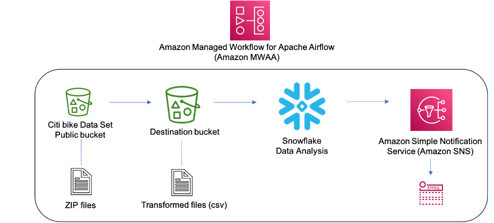
Solution Overview

The data used for transformation and analysis is based on the publicly available New York Citi Bike dataset. The data (zipped files), which includes rider demographics and trip data, is copied from the public Citi Bike Amazon Simple Storage Service (Amazon S3) bucket in your AWS account. Data is decompressed and stored in a different S3 bucket (transformed data can be stored in the same S3 bucket where data was ingested, but for simplicity, we’re using two separate S3 buckets). The transformed data is then made accessible to Snowflake for data analysis. The output of the queried data is published to Amazon Simple Notification Service (Amazon SNS) for consumption.

Amazon MWAA uses a directed acyclic graph (DAG) to run the workflows. In this post, we run three DAGs:

The following diagram illustrates this workflow.

DAG run workflow

See the GitHub repo for the DAGs and other files related to the post.

Note that in this post, we’re using a DAG to create a Snowflake connection, but you can also create the Snowflake connection using the Airflow UI or CLI.

Prerequisites

To deploy the solution, you should have a basic understanding of Snowflake and Amazon MWAA with the following prerequisites:

  • An AWS account in an AWS Region where Amazon MWAA is supported.
  • A Snowflake account with admin credentials. If you don’t have an account, sign up for a 30-day free trial. Select the Snowflake enterprise edition for the AWS Cloud platform.
  • Access to Amazon MWAA, Secrets Manager, and Amazon SNS.
  • In this post, we’re using two S3 buckets, called airflow-blog-bucket-ACCOUNT_ID and citibike-tripdata-destination-ACCOUNT_ID. Amazon S3 supports global buckets, which means that each bucket name must be unique across all AWS accounts in all the Regions within a partition. If the S3 bucket name is already taken, choose a different S3 bucket name. Create the S3 buckets in your AWS account. We upload content to the S3 bucket later in the post. Replace ACCOUNT_ID with your own AWS account ID or any other unique identifier. The bucket details are as follows:
    • airflow-blog-bucket-ACCOUNT_ID – The top-level bucket for Amazon MWAA-related files.
    • airflow-blog-bucket-ACCOUNT_ID/requirements – The bucket used for storing the requirements.txt file needed to deploy Amazon MWAA.
    • airflow-blog-bucket-ACCOUNT_ID/dags – The bucked used for storing the DAG files to run workflows in Amazon MWAA.
    • airflow-blog-bucket-ACCOUNT_ID/dags/mwaa_snowflake_queries – The bucket used for storing the Snowflake SQL queries.
    • citibike-tripdata-destination-ACCOUNT_ID – The bucket used for storing the transformed dataset.

When implementing the solution in this post, replace references to airflow-blog-bucket-ACCOUNT_ID and citibike-tripdata-destination-ACCOUNT_ID with the names of your own S3 buckets.

Set up the Amazon MWAA environment

First, you create an Amazon MWAA environment. Before deploying the environment, upload the requirements file to the airflow-blog-bucket-ACCOUNT_ID/requirements S3 bucket. The requirements file is based on Amazon MWAA version 2.6.3. If you’re testing on a different Amazon MWAA version, update the requirements file accordingly.

Complete the following steps to set up the environment:

  1. On the Amazon MWAA console, choose Create environment.
  2. Provide a name of your choice for the environment.
  3. Choose Airflow version 2.6.3.
  4. For the S3 bucket, enter the path of your bucket (s3:// airflow-blog-bucket-ACCOUNT_ID).
  5. For the DAGs folder, enter the DAGs folder path (s3:// airflow-blog-bucket-ACCOUNT_ID/dags).
  6. For the requirements file, enter the requirements file path (s3:// airflow-blog-bucket-ACCOUNT_ID/ requirements/requirements.txt).
  7. Choose Next.
  8. Under Networking, choose your existing VPC or choose Create MWAA VPC.
  9. Under Web server access, choose Public network.
  10. Under Security groups, leave Create new security group selected.
  11. For the Environment class, Encryption, and Monitoring sections, leave all values as default.
  12. In the Airflow configuration options section, choose Add custom configuration value and configure two values:
    1. Set Configuration option to secrets.backend and Custom value to airflow.providers.amazon.aws.secrets.secrets_manager.SecretsManagerBackend.
    2. Set Configuration option to secrets.backend_kwargs and Custom value to {"connections_prefix" : "airflow/connections", "variables_prefix" : "airflow/variables"}.                      Configuration options for secret manager
  13. In the Permissions section, leave the default settings and choose Create a new role.
  14. Choose Next.
  15. When the Amazon MWAA environment us available, assign S3 bucket permissions to the AWS Identity and Access Management (IAM) execution role (created during the Amazon MWAA install).

MWAA execution role
This will direct you to the created execution role on the IAM console.

For testing purposes, you can choose Add permissions and add the managed AmazonS3FullAccess policy to the user instead of providing restricted access. For this post, we provide only the required access to the S3 buckets.

  1. On the drop-down menu, choose Create inline policy.
  2. For Select Service, choose S3.
  3. Under Access level, specify the following:
    1. Expand List level and select ListBucket.
    2. Expand Read level and select GetObject.
    3. Expand Write level and select PutObject.
  4. Under Resources, choose Add ARN.
  5. On the Text tab, provide the following ARNs for S3 bucket access:
    1. arn:aws:s3:::airflow-blog-bucket-ACCOUNT_ID (use your own bucket).
    2. arn:aws:s3:::citibike-tripdata-destination-ACCOUNT_ID (use your own bucket).
    3. arn:aws:s3:::tripdata (this is the public S3 bucket where the Citi Bike dataset is stored; use the ARN as specified here).
  6. Under Resources, choose Add ARN.
  7. On the Text tab, provide the following ARNs for S3 bucket access:
    1. arn:aws:s3:::airflow-blog-bucket-ACCOUNT_ID/* (make sure to include the asterisk).
    2. arn:aws:s3:::citibike-tripdata-destination-ACCOUNT_ID /*.
    3. arn:aws:s3:::tripdata/* (this is the public S3 bucket where the Citi Bike dataset is stored, use the ARN as specified here).
  8. Choose Next.
  9. For Policy name, enter S3ReadWrite.
  10. Choose Create policy.
  11. Lastly, provide Amazon MWAA with permission to access Secrets Manager secret keys.

This step provides the Amazon MWAA execution role for your Amazon MWAA environment read access to the secret key in Secrets Manager.

The execution role should have the policies MWAA-Execution-Policy*, S3ReadWrite, and SecretsManagerReadWrite attached to it.

MWAA execution role policies

When the Amazon MWAA environment is available, you can sign in to the Airflow UI from the Amazon MWAA console using link for Open Airflow UI.

Airflow UI access

Set up an SNS topic and subscription

Next, you create an SNS topic and add a subscription to the topic. Complete the following steps:

  1. On the Amazon SNS console, choose Topics from the navigation pane.
  2. Choose Create topic.
  3. For Topic type, choose Standard.
  4. For Name, enter mwaa_snowflake.
  5. Leave the rest as default.
  6. After you create the topic, navigate to the Subscriptions tab and choose Create subscription.
    SNS topic
  7. For Topic ARN, choose mwaa_snowflake.
  8. Set the protocol to Email.
  9. For Endpoint, enter your email ID (you will get a notification in your email to accept the subscription).

By default, only the topic owner can publish and subscribe to the topic, so you need to modify the Amazon MWAA execution role access policy to allow Amazon SNS access.

  1. On the IAM console, navigate to the execution role you created earlier.
  2. On the drop-down menu, choose Create inline policy.
    MWAA execution role SNS policy
  3. For Select service, choose SNS.
  4. Under Actions, expand Write access level and select Publish.
  5. Under Resources, choose Add ARN.
  6. On the Text tab, specify the ARN arn:aws:sns:<<region>>:<<our_account_ID>>:mwaa_snowflake.
  7. Choose Next.
  8. For Policy name, enter SNSPublishOnly.
  9. Choose Create policy.

Configure a Secrets Manager secret

Next, we set up Secrets Manager, which is a supported alternative database for storing Snowflake connection information and credentials.

To create the connection string, the Snowflake host and account name is required. Log in to your Snowflake account, and under the Worksheets menu, choose the plus sign and select SQL worksheet. Using the worksheet, run the following SQL commands to find the host and account name.

Run the following query for the host name:

WITH HOSTLIST AS 
(SELECT * FROM TABLE(FLATTEN(INPUT => PARSE_JSON(SYSTEM$allowlist()))))
SELECT REPLACE(VALUE:host,'"','') AS HOST
FROM HOSTLIST
WHERE VALUE:type = 'SNOWFLAKE_DEPLOYMENT_REGIONLESS';

Run the following query for the account name:

WITH HOSTLIST AS 
(SELECT * FROM TABLE(FLATTEN(INPUT => PARSE_JSON(SYSTEM$allowlist()))))
SELECT REPLACE(VALUE:host,'.snowflakecomputing.com','') AS ACCOUNT
FROM HOSTLIST
WHERE VALUE:type = 'SNOWFLAKE_DEPLOYMENT';

Next, we configure the secret in Secrets Manager.

  1. On the Secrets Manager console, choose Store a new secret.
  2. For Secret type, choose Other type of secret.
  3. Under Key/Value pairs, choose the Plaintext tab.
  4. In the text field, enter the following code and modify the string to reflect your Snowflake account information:

{"host": "<<snowflake_host_name>>", "account":"<<snowflake_account_name>>","user":"<<snowflake_username>>","password":"<<snowflake_password>>","schema":"mwaa_schema","database":"mwaa_db","role":"accountadmin","warehouse":"dev_wh"}

For example:

{"host": "xxxxxx.snowflakecomputing.com", "account":"xxxxxx" ,"user":"xxxxx","password":"*****","schema":"mwaa_schema","database":"mwaa_db", "role":"accountadmin","warehouse":"dev_wh"}

The values for the database name, schema name, and role should be as mentioned earlier. The account, host, user, password, and warehouse can differ based on your setup.

Secret information

Choose Next.

  1. For Secret name, enter airflow/connections/snowflake_accountadmin.
  2. Leave all other values as default and choose Next.
  3. Choose Store.

Take note of the Region in which the secret was created under Secret ARN. We later define it as a variable in the Airflow UI.

Configure Snowflake access permissions and IAM role

Next, log in to your Snowflake account. Ensure the account you are using has account administrator access. Create a SQL worksheet. Under the worksheet, create a warehouse named dev_wh.

The following is an example SQL command:

CREATE OR REPLACE WAREHOUSE dev_wh 
 WITH WAREHOUSE_SIZE = 'xsmall' 
 AUTO_SUSPEND = 60 
 INITIALLY_SUSPENDED = true
 AUTO_RESUME = true
 MIN_CLUSTER_COUNT = 1
 MAX_CLUSTER_COUNT = 5;

For Snowflake to read data from and write data to an S3 bucket referenced in an external (S3 bucket) stage, a storage integration is required. Follow the steps defined in Option 1: Configuring a Snowflake Storage Integration to Access Amazon S3(only perform Steps 1 and 2, as described in this section).

Configure access permissions for the S3 bucket

While creating the IAM policy, a sample policy document code is needed (see the following code), which provides Snowflake with the required permissions to load or unload data using a single bucket and folder path. The bucket name used in this post is citibike-tripdata-destination-ACCOUNT_ID. You should modify it to reflect your bucket name.

{
  "Version": "2012-10-17",
  "Statement": [
    {
      "Effect": "Allow",
      "Action": [
        "s3:PutObject",
        "s3:GetObject",
        "s3:GetObjectVersion",
        "s3:DeleteObject",
        "s3:DeleteObjectVersion"
      ],
      "Resource": "arn:aws:s3::: citibike-tripdata-destination-ACCOUNT_ID/*"
    },
    {
      "Effect": "Allow",
      "Action": [
        "s3:ListBucket",
        "s3:GetBucketLocation"
      ],
      "Resource": "arn:aws:s3:::citibike-tripdata-destination-ACCOUNT_ID"
    }
  ]
}

Create the IAM role

Next, you create the IAM role to grant privileges on the S3 bucket containing your data files. After creation, record the Role ARN value located on the role summary page.

Snowflake IAM role

Configure variables

Lastly, configure the variables that will be accessed by the DAGs in Airflow. Log in to the Airflow UI and on the Admin menu, choose Variables and the plus sign.

Airflow variables

Add four variables with the following key/value pairs:

  • Key aws_role_arn with value <<snowflake_aws_role_arn>> (the ARN for role mysnowflakerole noted earlier)
  • Key destination_bucket with value <<bucket_name>> (for this post, the bucket used in citibike-tripdata-destination-ACCOUNT_ID)
  • Key target_sns_arn with value <<sns_Arn>> (the SNS topic in your account)
  • Key sec_key_region with value <<region_of_secret_deployment>> (the Region where the secret in Secrets Manager was created)

The following screenshot illustrates where to find the SNS topic ARN.

SNS topic ARN

The Airflow UI will now have the variables defined, which will be referred to by the DAGs.

Airflow variables list

Congratulations, you have completed all the configuration steps.

Run the DAG

Let’s look at how to run the DAGs. To recap:

  • DAG1 (create_snowflake_connection_blog.py) – Creates the Snowflake connection in Apache Airflow. This connection will be used to authenticate with Snowflake. The Snowflake connection string is stored in Secrets Manager, which is referenced in the DAG file.
  • DAG2 (create-snowflake_initial-setup_blog.py) – Creates the database, schema, storage integration, and stage in Snowflake.
  • DAG3 (run_mwaa_datapipeline_blog.py) – Runs the data pipeline, which will unzip files from the source public S3 bucket and copy them to the destination S3 bucket. The next task will create a table in Snowflake to store the data. Then the data from the destination S3 bucket will be copied into the table using a Snowflake stage. After the data is successfully copied, a view will be created in Snowflake, on top of which the SQL queries will be run.

To run the DAGs, complete the following steps:

  1. Upload the DAGs to the S3 bucket airflow-blog-bucket-ACCOUNT_ID/dags.
  2. Upload the SQL query files to the S3 bucket airflow-blog-bucket-ACCOUNT_ID/dags/mwaa_snowflake_queries.
  3. Log in to the Apache Airflow UI.
  4. Locate DAG1 (create_snowflake_connection_blog), un-pause it, and choose the play icon to run it.

You can view the run state of the DAG using the Grid or Graph view in the Airflow UI.

Dag1 run

After DAG1 runs, the Snowflake connection snowflake_conn_accountadmin is created on the Admin, Connections menu.

  1. Locate and run DAG2 (create-snowflake_initial-setup_blog).

Dag2 run

After DAG2 runs, the following objects are created in Snowflake:

  • The database mwaa_db
  • The schema mwaa_schema
  • The storage integration mwaa_citibike_storage_int
  • The stage mwaa_citibike_stg

Before running the final DAG, the trust relationship for the IAM user needs to be updated.

  1. Log in to your Snowflake account using your admin account credentials.
  2. Open your SQL worksheet created earlier and run the following command:
DESC INTEGRATION mwaa_citibike_storage_int;

mwaa_citibike_storage_int is the name of the integration created by the DAG2 in the previous step.

From the output, record the property value of the following two properties:

  • STORAGE_AWS_IAM_USER_ARN – The IAM user created for your Snowflake account.
  • STORAGE_AWS_EXTERNAL_ID – The external ID that is needed to establish a trust relationship.

Now we grant the Snowflake IAM user permissions to access bucket objects.

  1. On the IAM console, choose Roles in the navigation pane.
  2. Choose the role mysnowflakerole.
  3. On the Trust relationships tab, choose Edit trust relationship.
  4. Modify the policy document with the DESC STORAGE INTEGRATION output values you recorded. For example:
{
  "Version": "2012-10-17",
  "Statement": [
    {
      "Effect": "Allow",
      "Principal": {
        "AWS": "arn:aws:iam::5xxxxxxxx:user/mgm4-s- ssca0079"
      },
      "Action": "sts:AssumeRole",
      "Condition": {
        "StringEquals": {
          "sts:ExternalId": "AWSPARTNER_SFCRole=4_vsarJrupIjjJh77J9Nxxxx/j98="
        }
      }
    }
  ]
}

The AWS role ARN and ExternalId will be different for your environment based on the output of the DESC STORAGE INTEGRATION query

Trust relationship

  1. Locate and run the final DAG (run_mwaa_datapipeline_blog).

At the end of the DAG run, the data is ready for querying. In this example, the query (finding the top start and destination stations) is run as part of the DAG and the output can be viewed from the Airflow XCOMs UI.

Xcoms

In the DAG run, the output is also published to Amazon SNS and based on the subscription, an email notification is sent out with the query output.

Email

Another method to visualize the results is directly from the Snowflake console using the Snowflake worksheet. The following is an example query:

SELECT START_STATION_NAME,
COUNT(START_STATION_NAME) C FROM MWAA_DB.MWAA_SCHEMA.CITIBIKE_VW 
GROUP BY 
START_STATION_NAME ORDER BY C DESC LIMIT 10;

Snowflake visual

There are different ways to visualize the output based on your use case.

As we observed, DAG1 and DAG2 need to be run only one time to set up the Amazon MWAA connection and Snowflake objects. DAG3 can be scheduled to run every week or month. With this solution, the user examining the data doesn’t have to log in to either Amazon MWAA or Snowflake. You can have an automated workflow triggered on a schedule that will ingest the latest data from the Citi Bike dataset and provide the top start and destination stations for the given dataset.

Clean up

To avoid incurring future charges, delete the AWS resources (IAM users and roles, Secrets Manager secrets, Amazon MWAA environment, SNS topics and subscription, S3 buckets) and Snowflake resources (database, stage, storage integration, view, tables) created as part of this post.

Conclusion

In this post, we demonstrated how to set up an Amazon MWAA connection for authenticating to Snowflake as well as to AWS using AWS user credentials. We used a DAG to automate creating the Snowflake objects such as database, tables, and stage using SQL queries. We also orchestrated the data pipeline using Amazon MWAA, which ran tasks related to data transformation as well as Snowflake queries. We used Secrets Manager to store Snowflake connection information and credentials and Amazon SNS to publish the data output for end consumption.

With this solution, you have an automated end-to-end orchestration of your data pipeline encompassing ingesting, transformation, analysis, and data consumption.

To learn more, refer to the following resources:


About the authors

Payal Singh is a Partner Solutions Architect at Amazon Web Services, focused on the Serverless platform. She is responsible for helping partner and customers modernize and migrate their applications to AWS.

James Sun is a Senior Partner Solutions Architect at Snowflake. He actively collaborates with strategic cloud partners like AWS, supporting product and service integrations, as well as the development of joint solutions. He has held senior technical positions at tech companies such as EMC, AWS, and MapR Technologies. With over 20 years of experience in storage and data analytics, he also holds a PhD from Stanford University.

Bosco Albuquerque is a Sr. Partner Solutions Architect at AWS and has over 20 years of experience working with database and analytics products from enterprise database vendors and cloud providers. He has helped technology companies design and implement data analytics solutions and products.

Manuj Arora is a Sr. Solutions Architect for Strategic Accounts in AWS. He focuses on Migration and Modernization capabilities and offerings in AWS. Manuj has worked as a Partner Success Solutions Architect in AWS over the last 3 years and worked with partners like Snowflake to build solution blueprints that are leveraged by the customers. Outside of work, he enjoys traveling, playing tennis and exploring new places with family and friends.

Spark on AWS Lambda: An Apache Spark runtime for AWS Lambda

Post Syndicated from John Cherian original https://aws.amazon.com/blogs/big-data/spark-on-aws-lambda-an-apache-spark-runtime-for-aws-lambda/

Spark on AWS Lambda (SoAL) is a framework that runs Apache Spark workloads on AWS Lambda. It’s designed for both batch and event-based workloads, handling data payload sizes from 10 KB to 400 MB. This framework is ideal for batch analytics workloads from Amazon Simple Storage Service (Amazon S3) and event-based streaming from Amazon Managed Streaming for Apache Kafka (Amazon MSK) and Amazon Kinesis. The framework seamlessly integrates data with platforms like Apache Iceberg, Apache Delta Lake, Apache HUDI, Amazon Redshift, and Snowflake, offering a low-cost and scalable data processing solution. SoAL provides a framework that enables you to run data-processing engines like Apache Spark and take advantage of the benefits of serverless architecture, like auto scaling and compute for analytics workloads.

This post highlights the SoAL architecture, provides infrastructure as code (IaC), offers step-by-step instructions for setting up the SoAL framework in your AWS account, and outlines SoAL architectural patterns for enterprises.

Solution overview

Apache Spark offers cluster mode and local mode deployments, with the former incurring latency due to the cluster initialization and warmup. Although Apache Spark’s cluster-based engines are commonly used for data processing, especially with ACID frameworks, they exhibit high resource overhead and slower performance for payloads under 50 MB compared to the more efficient Pandas framework for smaller datasets. When compared to Apache Spark cluster mode, local mode provides faster initialization and better performance for small analytics workloads. The Apache Spark local mode on the SoAL framework is optimized for small analytics workloads, and cluster mode is optimized for larger analytics workloads, making it a versatile framework for enterprises.

We provide an AWS Serverless Application Model (AWS SAM) template, available in the GitHub repo, to deploy the SoAL framework in an AWS account. The AWS SAM template builds the Docker image, pushes it to the Amazon Elastic Container Registry (Amazon ECR) repository, and then creates the Lambda function. The AWS SAM template expedites the setup and adoption of the SoAL framework for AWS customers.

SoAL architecture

The SoAL framework provides local mode and containerized Apache Spark running on Lambda. In the SoAL framework, Lambda runs in a Docker container with Apache Spark and AWS dependencies installed. On invocation, the SoAL framework’s Lambda handler fetches the PySpark script from an S3 folder and submits the Spark job on Lambda. The logs for the Spark jobs are recorded in Amazon CloudWatch.

For both streaming and batch tasks, the Lambda event is sent to the PySpark script as a named argument. Utilizing a container-based image cache along with the warm instance features of Lambda, it was found that the overall JVM warmup time reduced from approx. 70 seconds to under 30 seconds. It was observed that the framework performs well with batch payloads up to 400 MB and streaming data from Amazon MSK and Kinesis. The per-session costs for any given analytics workload depends on the number of requests, the run duration, and the memory configured for the Lambda functions.

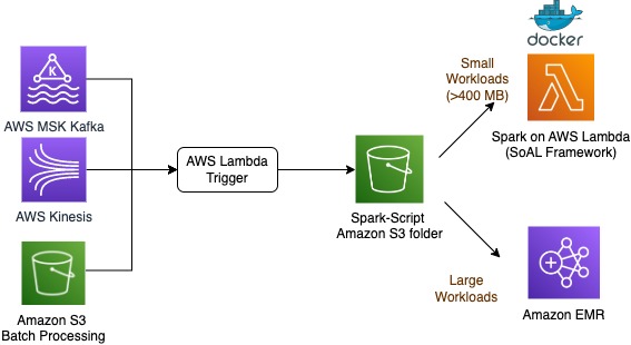
The following diagram illustrates the SoAL architecture.

Enterprise architecture

The PySpark script is developed in standard Spark and is compatible with the SoAL framework, Amazon EMR, Amazon EMR Serverless, and AWS Glue. If needed, you can use the PySpark scripts in cluster mode on Amazon EMR, EMR Serverless, and AWS Glue. For analytics workloads with a size between a few KBs and 400 MB, you can use the SoAL framework on Lambda and in larger analytics workload scenarios over 400 MB, and run the same PySpark script on AWS cluster-based tools like Amazon EMR, EMR Serverless, and AWS Glue. The extensible script and architecture make SoAL a scalable framework for analytics workloads for enterprises. The following diagram illustrates this architecture.

Prerequisites

To implement this solution, you need an AWS Identity and Access Management (IAM) role with permission to AWS CloudFormation, Amazon ECR, Lambda, and AWS CodeBuild.

Set up the solution

To set up the solution in an AWS account, complete the following steps:

  1. Clone the GitHub repository to local storage and change the directory within the cloned folder to the CloudFormation folder:
    git clone https://github.com/aws-samples/spark-on-aws-lambda.git

  2. Run the AWS SAM template sam-imagebuilder.yaml using the following command with the stack name and framework of your choice. In this example, the framework is Apache HUDI:
    sam deploy --template-file sam-imagebuilder.yaml --stack-name spark-on-lambda-image-builder --capabilities CAPABILITY_IAM CAPABILITY_NAMED_IAM --resolve-s3 --parameter-overrides 'ParameterKey=FRAMEWORK,ParameterValue=HUDI'

The command deploys a CloudFormation stack called spark-on-lambda-image-builder. The command runs a CodeBuild project that builds and pushes the Docker image with the latest tag to Amazon ECR. The command has a parameter called ParameterValue for each open-source framework (Apache Delta, Apache HUDI, and Apache Iceberg).

  1. After the stack has been successfully deployed, copy the ECR repository URI (spark-on-lambda-image-builder) that is displayed in the output of the stack.
  2. Run the AWS SAM Lambda package with the required Region and ECR repository:
    sam deploy --template-file sam-template.yaml --stack-name spark-on-lambda-stack --capabilities CAPABILITY_IAM CAPABILITY_NAMED_IAM --resolve-s3 --image-repository <accountno>.dkr.ecr.us-east-1.amazonaws.com/sparkonlambda-spark-on-lambda-image-builder --parameter-overrides 'ParameterKey=ScriptBucket,ParameterValue=<Provide the s3 bcucket of the script> ParameterKey=SparkScript,ParameterValue=<provide s3 folder lcoation> ParameterKey=ImageUri,ParameterValue=<accountno>.dkr.ecr.us-east-1.amazonaws.com/sparkonlambda-spark-on-lambda-image-builder:latest'

This command creates the Lambda function with the container image from the ECR repository. An output file packaged-template.yaml is created in the local directory.

  1. Optionally, to publish the AWS SAM application to the AWS Serverless Application Repository, run the following command. This allows AWS SAM template sharing with the GUI interface using AWS Serverless Application Repository and other developers to use quick deployments in the future.
    sam publish --template packaged-template.yaml

After you run this command, a Lambda function is created using the SoAL framework runtime.

  1. To test it, use PySpark scripts from the spark-scripts folder. Place the sample script and accomodations.csv dataset in an S3 folder and provide the location via the Lambda environment variables SCRIPT_BUCKET and SCRIPT_LOCATION.

After Lambda is invoked, it uploads the PySpark script from the S3 folder to a container local storage and runs it on the SoAL framework container using SPARK-SUBMIT. The Lambda event is also passed to the PySpark script.

Clean up

Deploying an AWS SAM template incurs costs. Delete the Docker image from Amazon ECR, delete the Lambda function, and remove all the files or scripts from the S3 location. You can also use the following command to delete the stack:

sam delete --stack-name spark-on-lambda-stack

Conclusion

The SoAL framework enables you to run Apache Spark serverless tasks on AWS Lambda efficiently and cost-effectively. Beyond cost savings, it ensures swift processing times for small to medium files. As a holistic enterprise vision, SoAL seamlessly bridges the gap between big and small data processing, using the power of the Apache Spark runtime across both Lambda and other cluster-based AWS resources.

Follow the steps in this post to use the SoAL framework in your AWS account, and leave a comment if you have any questions.


About the authors

John Cherian is Senior Solutions Architect(SA) at Amazon Web Services helps customers with strategy and architecture for building solutions on AWS.

Emerson Antony is Senior Cloud Architect at Amazon Web Services helps customers with implementing AWS solutions.

Kiran Anand is Principal AWS Data Lab Architect at Amazon Web Services helps customers with Big data & Analytics architecture.

A phased approach towards a complex HITRUST r2 validated assessment

Post Syndicated from Abdul Javid original https://aws.amazon.com/blogs/security/a-phased-approach-towards-a-complex-hitrust-r2-validated-assessment/

Health Information Trust Alliance (HITRUST) offers healthcare organizations a comprehensive and standardized approach to information security, privacy, and compliance. HITRUST Common Security Framework (HITRUST CSF) can be used by organizations to establish a robust security program, ensure patient data privacy, and assist with compliance with industry regulations. HITRUST CSF enhances security, streamlines compliance efforts, reduces risk, and contributes to overall security resiliency and the trustworthiness of healthcare entities in an increasingly challenging cybersecurity landscape.

While HITRUST primarily focuses on the healthcare industry, its framework and certification program are adaptable and applicable to other industries. The HITRUST CSF is a set of controls and requirements that organizations must comply with to achieve HITRUST certification. The HITRUST R2 assessment is the process by which organizations are evaluated against the requirements of the HITRUST CSF. During the assessment, an independent third party assessor examines the organization’s technical security controls, operational policies and procedures, and the implementation of all controls to determine if they meet the specified HITRUST requirements.

HITRUST r2 validated assessment certification is a comprehensive process that involves meeting numerous assessment requirements. The number of requirements can vary significantly, ranging from 500 to 2,000 depending on your environment’s risk factors and regulatory requirements. Attempting to address all of these requirements simultaneously especially when migrating systems to Amazon Web Services (AWS) can be overwhelming. By using a strategy of separating your compliance journey into environments and applications, you can streamline the process and achieve HITRUST compliance more efficiently and within a realistic timeframe.

In this blog post, we start by exploring the HITRUST domain structure, highlighting the security objective of each domain. We then show how you can use AWS configurable services to help meet these objectives.

Lastly, we present a simple and practical reference architecture with an AWS multi-account implementation that you can use as the foundation for hosting your AWS application, highlighting the phased approach for HITRUST compliance. Please note that this blog is intended to assist with using AWS services in a manner that supports an organization’s HITRUST compliance, but a HITRUST assessment is at an organizational level and involves controls that extend beyond the organization’s use of AWS.

HITRUST certification journey – Scope applications systems on AWS infrastructure:

The HITRUST controls needed for certification are structured within 19 HITRUST domains, covering a wide range of technical and administrative control requirements. To efficiently manage the scope of your certification assessment, start by focusing on the AWS landing zone, which serves as a critical foundational infrastructure component for running applications. When establishing the AWS landing zone, verify that it aligns with the AWS HITRUST security control requirements that are dependent on the scope of your assessment. Note that these 19 domains are a combination of technical controls and foundational administrative controls.

After you’ve set up a HITRUST compliant landing zone, you can begin evaluating your applications for HITRUST compliance as you migrate them to AWS. When you expand and migrate applications to the HITRUST-certified AWS landing zone assessed by your third party assessor, you can inherit the HITRUST controls required for application assessment directly from the landing zone. This simplifies and narrows the scope of your assessment activities.

Figure 1 that follows shows the two key phases and how a bottom-up phased approach can be structured with related HITRUST controls.

Figure 1: HITRUST Phase 1 and Phase 2 high-level components

Figure 1: HITRUST Phase 1 and Phase 2 high-level components

The diagram illustrates:

  • An AWS landing zone environment as Phase 1 and its related HITRUST domain controls
  • An application system as Phase 2 and its related application system specific controls

HITRUST domain security objectives:

The HITRUST CSF based certification consists of 19 domains, which are broad categories that encompass various aspects of information security and privacy controls. These domains serve as a framework for your organization to assess and enhance its security posture. These domains cover a wide range of controls and practices related to information security, privacy, risk management, and compliance. Each domain consists of a set of control objectives and requirements that your organization must meet to achieve HITRUST certification.

The following table lists each domain, the key security objectives expected, and the AWS configurable services relevant to the security objectives. These are listed as a reference to give you an idea of the scope of each domain; the actual services and tools to meet specific HITRUST requirements will vary depending upon your scope and its HITRUST requirements.

Note: The information in this post is a general guideline and recommendation based on a phased approach for HITRUST r2 validated assessment. The examples are based on the information available at the time of publication and are not a full solution.

HITRUST domains, security objectives, and related AWS services

HITRUST domain Summary of key security objectives expected in HITRUST domains Related AWS configurable services
1. Information Protection Program
  • Implement information security management program.
  • Verify role suitability for employees, contractors, and third-party users.
  • Provide management guidance aligned with business goals and regulations.
  • Safeguard an organization’s information and assets.
  • Enhance awareness of information security among stakeholders.
AWS Artifact
AWS Service Catalog
AWS Config
Amazon Cybersecurity Awareness Training
2. Endpoint Protection
  • Protect information and software from unauthorized or malicious code.
  • Safeguard information in networks and the supporting network infrastructure
AWS Systems Manager
AWS Config
Amazon Inspector
AWS Shield
AWS WAF
3. Portable Media Security
  • Ensure the protection of information assets, prevent unauthorized disclosure, alteration, deletion, or harm, and maintain uninterrupted business operations.
AWS Identity and Access Management (IAM)
Amazon Simple Storage Service (Amazon S3)
AWS Key Management Service (AWS KMS)
AWS CloudTrail
Amazon Macie
Amazon Cognito
Amazon Workspaces Family
4. Mobile Device Security
  • Ensure information security while using mobile computing devices and remote work facilities.
AWS Database Migration Service (AWS DMS)
AWS IoT Device Defender
AWS Snowball
AWS Config
5. Wireless Security
  • Ensure the safeguarding of information within networks and the security of the underlying network infrastructure.
AWS Certificate Manager (ACM)
6. Configuration Management
  • Ensure adherence to organizational security policies and standards for information systems.
  • Control system files, access, and program source code for security.
  • Document, maintain, and provide operating procedures to users.
  • Strictly control project and support environments for secure development of application system software and information.
AWS Config
AWS Trusted Advisor
Amazon CloudWatch
AWS Security Hub
Systems Manager
7. Vulnerability Management
  • Implement effective and repeatable technical vulnerability management to mitigate risks from exploited vulnerabilities.
  • Establish ownership and defined responsibilities for the protection of information assets within management.
  • Design controls in applications, including user-developed ones, to prevent errors, loss, unauthorized modification, or misuse of information. These controls should encompass input data validation, internal processing, and output data.
Amazon Inspector
CloudWatch
Security Hub
8. Network Protection
  • Secure information across networks and network infrastructure.
  • Prevent unauthorized access to networked services.
  • Ensure unauthorized access prevention to information in application systems.
  • Implement controls within applications to prevent errors, loss, unauthorized modification, or misuse of information.
Amazon Route 53
AWS Control Tower
Amazon Virtual Private Cloud (Amazon VPC)
AWS Transit Gateway
Network Load Balancer
AWS Direct Connect
AWS Site-to-Site VPN
AWS CloudFormation
AWS WAF
ACM
9. Transmission Protection
  • Ensure robust protection of information within networks and their underlying infrastructure.
  • Facilitate secure information exchange both internally and externally, adhering to applicable laws and agreements.
  • Ensure the security of electronic commerce services and their use.
  • Employ cryptographic methods to ensure confidentiality, authenticity, and integrity of information.
  • Formulate cryptographic control policies and institute key management to bolster their implementation.
Systems Manager
ACM
10. Password Management
  • Register, track, and periodically validate authorized user accounts to prevent unauthorized access to information systems.
AWS Secrets Manager, Systems Manager Parameter Store, AWS KMS
11. Access Control
  • Monitor and log security events to detect unauthorized activities in compliance with legal requirements.
  • Prevent unauthorized access, compromise, or theft of information, assets, and user entry.
  • Safeguard against unauthorized access to networked services, operating systems, and application information.
  • Manage access rights and asset recovery for terminated or transferred personnel and contractors.
  • Ensure adherence to applicable laws, regulations, contracts, and security requirements throughout information systems’ lifecycle.
IAM
AWS Resource Access Manager (AWS RAM)
Amazon GuardDuty
AWS Identity Center
12. Audit Logging & Monitoring
  • Comply with laws, regulations, contracts, and security mandates in information systems’ design, operation, use, and management.
  • Document, maintain, and share operating procedures with relevant users.
  • Monitor, record, and uncover unauthorized information processing in line with legal requirements.
AWS Control Tower
Amazon S3
CloudTrail
GuardDuty
AWS Config
CloudWatch
Amazon VPC Flow logs
Amazon OpenSearch Service
13. Education, Training and Awareness
  • Secure information when using mobile devices and teleworking.
  • Make employees, contractors, and third-party users aware of security threats, and responsibilities and reduce human error.
  • Ensure information systems comply with laws, regulations, contracts, and security requirements.
  • Assign ownership and defined responsibilities for protecting information assets.
  • Protect information and software integrity from unauthorized code.
  • Securely exchange information within and outside the organization, following relevant laws and agreements.
  • Develop strategies to counteract business interruptions, protect critical processes, and resume them promptly after system failures or disasters.
Security Hub
Amazon Cybersecurity Awareness Training
Trusted Advisor
14. Third-Party Assurance
  • Safeguard information and assets by mitigating risks linked to external products or services.
  • Verify third-party service providers adhere to security requirements and maintain agreed upon service levels.
  • Enforce stringent controls over development, project, and support environments to ensure software and information security.
AWS Artifact
AWS Service Organization Controls (SOC) Reports
ISO27001 reports
15. Incident Management
  • Address security events and vulnerabilities promptly for timely correction.
  • Foster awareness among employees, contractors, and third-party users to reduce human errors.
  • Consistently manage information security incidents for effective response.
  • Handle security events to facilitate timely corrective measures.
AWS Incident Detection and Response
Security Hub
Amazon Inspector
CloudTrail
AWS Config
Amazon Simple Notification Service (Amazon SNS)
GuardDuty
AWS WAF
Shield
CloudFormation
16. Business Continuity & Disaster Recovery
  • Maintain, protect, and make organizational information available.
  • Develop strategies and plans to prevent disruptions to business activities, safeguard critical processes from system failures or disasters, and ensure their prompt recovery.
AWS Backup & Restore
CloudFormation
Amazon Aurora
CrossRegion replication
AWS Backup
Disaster Recovery: Pilot Light, Warm Standby, Multi Site Active-Active
17. Risk Management
  • Integrate security as a vital element within information systems.
  • Develop and implement a risk management program encompassing risk assessment, mitigation, and evaluation
Trusted Advisor
AWS Config Rules
18. Physical & Environmental Security
  • Secure the organization’s premises and information from unauthorized physical access, damage, and interference.
  • Prevent unauthorized access to networked services.
  • Safeguard assets, prevent loss, damage, theft, or compromise, and ensure uninterrupted organizational activities.
  • Protect information assets from unauthorized disclosure, modification, removal, or destruction, and prevent interruptions to business activities.
AWS Data Centers
Amazon CloudFront
AWS Regions and Global Infrastructure
19. Data Protection & Privacy
  • Ensure the security of the organization’s information and assets when using external products or services.
  • Ensure planning, operation, use, and control of information systems align with applicable laws, regulations, contracts, and security requirements.
Amazon S3
AWS KMS
Aurora
OpenSearch Service
AWS Artifact
Macie

Note: You can use AWS HITRUST-certified services to support your HITRUST compliance requirements. Use of these services in their default state doesn’t automatically ensure HITRUST certifiability. You must demonstrate compliance through formal formulation of policies, procedures, and implementation tailored to your scope, which involves configuring and customizing AWS HITRUST certified services to align precisely with HITRUST requirements within your scope and involves implementation of controls outside of the scope of the use of AWS services (such as appropriate organization-wide policies and procedures).

HITRUST phased approach – Reference architecture:

Figure 2 shows the recommended HITRUST Phase 1 and Phase 2 accounts and components within a landing zone.

Figure 2: HITRUST Phases 1 and 2 architecture including accounts and components

Figure 2: HITRUST Phases 1 and 2 architecture including accounts and components

The reference architecture shown in Figure 2 illustrates:

  • A high-level structure of AWS accounts arranged in HITRUST Phase 1 and Phase 2
  • The accounts in HITRUST Phase 1 include:
    • Management account: The management account in the AWS landing zone is the primary account responsible for governing and managing the entire AWS environment.
    • Security account: The security account is dedicated to security and compliance functions, providing a centralized location for security-related tools and monitoring.
    • Central logging account: This account is designed for centralized logging and storage of logs from all other accounts, aiding in security analysis and troubleshooting.
    • Central audit: The central audit account is used for compliance monitoring, logging audit events, and verifying adherence to security standards.
    • DevOps account: DevOps accounts are used for software development and deployment, enabling continuous integration and delivery (CI/CD) processes.
    • Networking account: Networking accounts focus on network management, configuration, and monitoring to support reliable connectivity within the AWS environment.
    • DevSecOps account: DevSecOps accounts combine development, security, and operations to embed security practices throughout the software development lifecycle.
    • Shared services account: Shared services accounts host common resources, such as IAM services, that are shared across other accounts for centralized management.

The account group for HITRUST Phase 2 includes:

  • Tenant A – sample application workloads
  • Tenant B – sample application workloads

HITRUST Phase 1 – HITRUST foundational landing zone assessment phase:

In this phase you define the scope of assessment, including the specific AWS landing zone components and configurations that must be HITRUST compliant. The primary focus here is to evaluate the foundational infrastructure’s compliance with HITRUST controls. This involves a comprehensive review of policies and procedures, and implementation of all requirements within the landing zone scope. Assessing this phase separately enables you to verify that your foundational infrastructure adheres to HITRUST controls. Some of the policies, procedures, and configurations that are HITRUST assessed in this phase can be inherited across multiple applications’ assessments in later phases. Assessing this infrastructure once and then inheriting these controls for applications can be more efficient than assessing each application individually.

By establishing a secure and compliant foundation at the start, you can plan application assessments in later phases, making it simpler for subsequent applications to adhere to HITRUST requirements. This can streamline the compliance process and reduce the overall time and effort required. By assessing the landing zone separately, you can identify and address compliance gaps or issues in your foundational infrastructure, reducing the risk of non-compliance for the applications built upon it. Use the following high-level technical approach for this phase of assessment.

  1. Build your AWS landing zone with HITRUST controls. See Building a landing zone for more information.
  2. Use AWS and configure services according to the HITRUST requirements that are applicable to your infrastructure scope.
  3. The HITRUST on AWS Quick Start guide is a reference for building HITRUST with one account. You can use the guide as a starting point to build a multi account architecture.

HITRUST Phase 2 – HITRUST application assessment phase:

During this phase, you examine your AWS workload application accounts to conduct HITRUST assessments for application systems that are running within the AWS landing zone. You have the option to inherit environment-related controls that have been certified as HITRUST compliant within the landing zone in the previous phase.

The following key steps are recommended in this phase:

  1. Readiness assessment for application scope: Conduct a thorough readiness assessment focused on the application scope, and define boundaries with scoped applications (AWS workload accounts).
  2. HITRUST application controls: Gather specific HITRUST requirements for application scope by creating a HITRUST object for the application scope.
  3. Scoped requirements analysis: Analyze requirements and use requirements that can be inherited from Phase 1 of the infrastructure assessment.
  4. Gap analysis: Work with subject matter experts to conduct a gap analysis, and develop policies, procedures, and implementations for application specific controls.
  5. Remediation: Remediate the gaps identified during the gap analysis activity.
  6. Formal r2 assessment: Work with a third-party assessor to initiate a formal r2 validated assessment with HITRUST.

Conclusion

By breaking the compliance process into distinct phases, you can concentrate your resources on specific areas and prioritize essential assets accordingly. This approach supports a focused strategy, systematically addressing critical controls, and helping you to fulfill compliance requirements in a scalable manner. Obtaining the initial certification for the infrastructure and platform layers establishes a robust foundational architecture for subsequent phases, which involve application systems.

Earning certification at each phase provides tangible evidence of progress in your compliance journey. This achievement instills confidence in both internal and external stakeholders, affirming your organization’s commitment to security and compliance.

For guidance on achieving, maintaining, and automating compliance in the cloud, reach out to AWS Security Assurance Services (AWS SAS) or your account team. AWS SAS is a PCI QSAC and HITRUST External Assessor that can help by tying together applicable audit standards to AWS service-specific features and functionality. They can help you build on frameworks such as PCI DSS, HITRUST CSF, NIST, SOC 2, HIPAA, ISO 27001, GDPR, and CCPA.

If you have feedback about this post, submit comments in the Comments section below. If you have questions about this post, start a new thread on the AWS Security, Identity, & Compliance re:Post or contact AWS Support.

Want more AWS Security news? Follow us on Twitter.

Abdul Javid

Abdul Javid

Abdul is a Senior Security Assurance Consultant and PCI DSS Qualified Security Assessor with AWS Security Assurance Services, and has more than 25 years of IT governance, operations, security, risk, and compliance experience. Abdul leverages his experience and knowledge to advise AWS customers with guidance and advice on their compliance journey. Abdul earned an M.S. in Computer Science from IIT, Chicago and holds various industry recognized sought after certifications in security and program and risk management from prominent organizations like AWS, HITRUST, ISACA, PMI, PCI DSS, and ISC2.

Cate Ciccolone

Cate Ciccolone

Cate is a Senior Security Consultant for Amazon Web Services (AWS) where she provides technical and advisory consulting services to global healthcare organizations to help them secure their regulated workloads, minimize risk, and meet compliance goals. Her experience spans cybersecurity engineering, healthcare compliance, electronic health record architecture, and clinical application security. Cate is an AWS Certified Solutions Architect and holds several certifications including EC-Council Certified Incident Handler (E|CIH) and HITRUST Certified Practitioner (CCSFP).

Simplify Amazon Redshift monitoring using the new unified SYS views

Post Syndicated from Urvish Shah original https://aws.amazon.com/blogs/big-data/simplify-amazon-redshift-monitoring-using-the-new-unified-sys-views/

Amazon Redshift is a fully managed, petabyte-scale data warehouse service in the cloud, providing up to five times better price-performance than any other cloud data warehouse, with performance innovation out of the box at no additional cost to you. Tens of thousands of customers use Amazon Redshift to process exabytes of data every day to power their analytics workloads.

In this post, we discuss Amazon Redshift SYS monitoring views and how they simplify the monitoring of your Amazon Redshift workloads and resource usage.

Overview of SYS monitoring views

SYS monitoring views are system views in Amazon Redshift that can be used to monitor query and workload resource usage for provisioned clusters as well as for serverless workgroups. They offer the following benefits:

  • They’re categorized based on functional alignment, considering query state, performance metrics, and query types
  • We have introduced new performance metrics like planning_time, lock_wait_time, remote_read_io, and local_read_io to aid in performance troubleshooting
  • It improves the usability of monitoring views by logging the user-submitted query instead of the Redshift optimizer-rewritten query
  • It provides more troubleshooting metrics using fewer views
  • It enables unified Amazon Redshift monitoring by enabling you to use the same query across provisioned clusters or serverless workgroups

Let’s look at some of the features of SYS monitoring views and how they can be used for monitoring.

Unify various query-level monitoring metrics

The following table shows how you can unify various metrics and information for a query from multiple system tables & views into one SYS monitoring view.

STL/SVL/STV Information element SYS Monitoring View View columns
STL_QUERY elapsed time, query label, user ID, transaction, session, label, stopped queries, database name SYS_QUERY_HISTORY

user_id

query_id

query_label

transaction_id

session_id

database_name

query_type

status

result_cache_hit

start_time

end_time

elapsed_time

queue_time

execution_time

error_message

returned_rows

returned_bytes

query_text

redshift_version

usage_limit

compute_type

compile_time

planning_time

lock_wait_time

STL_WLM_QUERY queue time, runtime
SVL_QLOG result cache
STL_ERROR error code, error message
STL_UTILITYTEXT non-SELECT SQL
STL_DDLTEXT DDL statements
SVL_STATEMENTEXT all types of SQL statements
STL_RETURN return rows and bytes
STL_USAGE_CONTROL usage limit
STV_WLM_QUERY_STATE current state of WLM
STV_RECENTS recent and in-flight queries
STV_INFLIGHT in-flight queries
SVL_COMPILE compilation

For additional information on SYS to STL/SVL/STV mapping, refer to Migrating to SYS monitoring views.

User query-level logging

To enhance query performance, the Redshift query engine can rewrite user-submitted queries. The user-submitted query identifier is different than the rewritten query identifier. We refer to the user-submitted query as the parent query and the rewritten query as the child query in this post.

The following diagram illustrates logging at the parent query level and child query level. The parent query identifier is 1000, and the child query identifiers are 1001, 1002, and 1003.

Query lifecycle timings

SYS_QUERY_HISTORY has an enhanced list of columns to provide granular time metrics relating to the different query lifecycle phases. Note all times are recorded in microseconds. The following table summarizes these metrics.

Time metrics Description
planning_time The time the query spent prior to running the query, which typically includes query lifecycle phases like parse, analyze, planning and rewriting.
lock_wait_time The time the query spent on acquiring the locks on the required database objects referenced.
queue_time The time the query spent in the queue waiting for resources to be available to run.
compile_time The time the query spent compiling.
execution_time The time the query spent running. In the case of a SELECT query, this also includes the return time.
elapsed_time The end-to-end time of the query run.

Solution overview

We discuss the following scenarios to help gain familiarity with the SYS monitoring views:

  • Workload and query lifecycle monitoring
  • Data ingestion monitoring
  • External query monitoring
  • Slow query performance troubleshooting

Prerequisites

You should have the following prerequisites to follow along with the examples in this post:

Additionally, download all the SQL queries that are referenced in this post as Redshift Query Editor v2 SQL notebooks.

Workload and query lifecycle monitoring

In this section, we discuss how to monitor the workload and query lifecycle.

Identify in-flight queries

SYS_QUERY_HISTORY provides a singular view to look at all the in-flight queries as well as historical runs. See the following example query:

SELECT  
  *
FROM    
  sys_query_history
WHERE    status IN ('planning', 'queued', 'running', 'returning')
ORDER BY
  start_time;

We get the following output.

Identify top long-running queries

The following query helps retrieve the top 100 queries that are taking the longest to run. Analyzing (and, if feasible, optimizing) these queries can help improve overall performance. These metrics are accumulated statistics across all runs of the query. Note that all the time values are in microseconds.

--top long running query by elapsed_time
SELECT  
  user_id
  , transaction_id
  , query_id
  , database_name
  , query_type
  , query_text::VARCHAR(100)
  , lock_wait_time
  , planning_time
  , compile_time
  , execution_time
  , elapsed_time
FROM    
  sys_query_history
ORDER BY
  elapsed_time DESC
LIMIT 100;

We get the following output.

Gather daily counts of queries by query types, period, and status

The following query provides insight into the distribution of different types of queries across different days and helps evaluate and track any changes in the workload:

--daily breakdown of workload by query types and status
SELECT  
  DATE_TRUNC('day', start_time) period_daily
  , query_type
  , status
  , COUNT(*)
FROM    
  sys_query_history
GROUP BY
  period_daily
  , query_type
  , status
ORDER BY
  period_daily
  , query_type
  , status;

We get the following output.

Gather run details of an in-flight query

To determine the run-level details of a query that is in-flight, you can use the is_active = ‘t’ filter when querying the SYS_QUERY_DETAIL table. See the following example:

SELECT  
  query_id
  , child_query_sequence
  , stream_id
  , segment_id
  , step_id
  , step_name
  , table_id
  , coalesce(table_name,'')|| coalesce(source,'') as table_name
  , start_time
  , end_time
  , duration
  , blocks_read
  , local_read_io
  , remote_read_io
FROM    
  sys_query_detail
WHERE is_active = 't'
ORDER BY
  query_id
  , child_query_sequence
  , stream_id
  , segment_id
  , step_id;

To view the latest 100 COPY queries run, use the following code:

SELECT  
  session_id
  , transaction_id
  , query_id
  , database_name
  , table_name
  , data_source
  , loaded_rows
  , loaded_bytes
  , duration / 1000.00 duration_ms
FROM    
  sys_load_history
ORDER BY
  start_time DESC LIMIT 100;

We get the following output.

Gather transaction-level details for commits and undo

SYS_TRANSACTION_HISTORY provides transaction-level logging by providing insights into committed transactions with details like blocks committed, status, and isolation level (serializable or snapshot used). It also logs details about the rolled back or undo transactions.

The following screenshots illustrate fetching details about a transaction that was committed successfully.

The following screenshots illustrate fetching details about a transaction that was rolled back.

Stats and vacuum

The SYS_ANALYZE_HISTORY monitoring view provides details like the last timestamp of analyze queries, the duration for which a particular analyze query ran, the number of rows in the table, and the number of rows modified. The following example query provides a list of the latest analyze queries that ran for all the permanent tables:

SELECT  
  TRIM(schema_name) schema_name
  , TRIM(table_name) table_name
  , table_id
  , status
  , COUNT(*) times_analyze_was_triggered
  , MAX(last_analyze_time) last_analyze_time
  , MAX(end_time) end_time
  , AVG(ROWS) "rows"
  , AVG(modified_rows) modified_rows
FROM    
  sys_analyze_history
WHERE
   status != 'Skipped'
GROUP BY
  schema_name
  , table_name
  , table_id
  , status
ORDER BY
  schema_name
  , table_name
  , table_id
  , status
  , end_time;

We get the following output.

The SYS_VACUUM_HISTORY monitoring view provides a complete set of details on VACUUM in a single view. For example, see the following code:

SELECT  
  user_id
  , transaction_id
  , query_id
  , TRIM(database_name) as database_name
  , TRIM(schema_name) as schema_name
  , TRIM(table_name) table_name
  , table_id
  , vacuum_type
  , is_automatic as is_auto
  , duration
  , rows_before_vacuum
  , size_before_vacuum
  , reclaimable_rows
  , reclaimed_rows
  , reclaimed_blocks
  , sortedrows_before_vacuum
  , sortedrows_after_vacuum
FROM    
  sys_vacuum_history
WHERE    status LIKE '%Finished%'
ORDER BY
  start_time;

We get the following output.

Data ingestion monitoring

In this section, we discuss how to monitor data ingestion.

Summary of ingestion

SYS_LOAD_HISTORY provides details into the statistics of COPY commands. Use this view for summarized insights into your ingestion workload. The following example query provides an hourly summary of ingestion broken down by tables in which data was ingested:

SELECT  
  date_trunc('hour', start_time) period_hourly
  , database_name
  , table_name
  , status
  , file_format
  , SUM(loaded_rows) total_rows_ingested
  , SUM(loaded_bytes) total_bytes_ingested
  , SUM(source_file_count) num_of_files_to_process
  , SUM(file_count_scanned) num_of_files_processed
  , SUM(error_count) total_errors
FROM    
  sys_load_history
GROUP BY
  period_hourly
  , database_name
  , table_name
  , status
  , file_format
ORDER BY
  table_name
  , period_hourly
  , status;

We get the following output.

File-level ingress logging

SYS_LOAD_DETAIL provides more granular insights into how ingestion is performed at the file level. For example, see the following query using sys_load_history:

SELECT  
  *
FROM    
  sys_load_history
WHERE table_name = 'catalog_sales'
ORDER BY
  start_time;

We get the following output.

The following example shows what detailed file-level monitoring looks like:

 SELECT  
  user_id
  , query_id
  , TRIM(file_name) file_name
  , bytes_scanned
  , lines_scanned
  , splits_scanned
  , record_time
  , start_time
  , end_time
FROM    
  sys_load_detail
WHERE query_id = 1824870
ORDER BY
  start_time;

Check for errors during ingress process

SYS_LOAD_ERROR_DETAIL enables you to track and troubleshoot errors that may have occurred during the ingestion process. This view logs details for the file that encountered the error during the ingestion process along with the line number at which the error occurred and column details within that line. See the following code:

select * from sys_load_error_detail order by start_time limit 100;

We get the following output.

External query monitoring

SYS_EXTERNAL_QUERY_DETAIL provides run details for external queries, which includes Amazon Redshift Spectrum and federated queries. This view logs details at the segment level and provides useful insights to troubleshoot and monitor performance of external queries in a single monitoring view. The following are a few useful metrics and data points this monitoring view provides:

  • Number of external files scanned (scanned_files) and format of external files (file_format) such as Parquet, text file, and so on
  • Data scanned in terms of rows (returned_rows) and bytes (returned_bytes)
  • Usage of partitioning (total_partitions and qualified_partitions) by external queries and tables
  • Granular insights into time taken in listing (s3list_time) and qualifying partitions (get_partition_time) for a given external object
  • External file location (file_location) and external table name (table_name)
  • Type of external source (source_type), such as Amazon Simple Storage Service (Amazon S3) for Redshift Spectrum, or federated
  • Recursive scan for subdirectories (is_recursive) or access of nested column data type (is_nested)

For example, the following query shows the daily summary of the number of external queries run and data scanned:

SELECT  
  DATE_TRUNC('hour', start_time) period_hourly
  , user_id
  , TRIM(source_type) source_type
  , COUNT (DISTINCT query_id) query_counts
  , SUM(returned_rows) returned_rows
  , ROUND(SUM(returned_bytes) / 1024^3,2) returned_gb
FROM    
  sys_external_query_detail
GROUP BY
  period_hourly
  , user_id
  , source_type
ORDER BY
  period_hourly
  , user_id
  , source_type;

We get the following output.

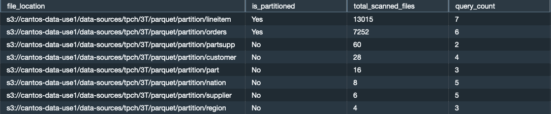
Usage of partitions

You can verify whether the external queries scanning large sums of data and files are partitioned or not. When you use partitions, you can restrict the amount of data that your external query has to scan by pruning based on the partition key. See the following code:

SELECT  
  file_location
  , CASE
      WHEN NVL(total_partitions,0) = 0
      THEN 'No'
      ELSE 'Yes'
    END is_partitioned
  , SUM(scanned_files) total_scanned_files
  , COUNT(DISTINCT query_id) query_count
FROM    
  sys_external_query_detail
GROUP BY
  file_location
  , is_partitioned
ORDER BY
  total_scanned_files DESC;

We get the following output.

For any errors encountered with external queries, look into SYS_EXTERNAL_QUERY_ERROR, which logs details at the granularity of file_location, column, and rowid within that file.

Slow query performance troubleshooting

Refer to the sysview_slow_query_performance_troubleshooting SQL notebook downloaded as part of the prerequisites for a step-by-step guide on how to perform query-level troubleshooting using SYS monitoring views and find answers to the following questions:

  • Do the queries being compared have similar query text?
  • Did the query use the result cache?
  • Which parts of the query lifecycle (queuing, compilation, planning, lock wait) are contributing the most to query runtimes?
  • Has the query plan changed?
  • Is the query reading more data blocks?
  • Is the query spilling to disk? If so, is it spilling to local or remote storage?
  • Is the query highly skewed with respect to data (distribution) and time (runtime)?
  • Do you see more rows processed in join steps or nested loops?
  • Are there any alerts indicating staleness in statistics?
  • When was the last vacuum and analyze performed for the tables involved in the query?

Clean up

If you created any Redshift provisioned clusters or Redshift Serverless workgroups as part of this post and no longer need them for your workloads, you can delete them to avoid incurring additional costs.

Conclusion

In this post, we explained how you can use the Redshift SYS monitoring views to monitor workloads of provisioned clusters and serverless workgroups. The SYS monitoring views provide simplified monitoring of the workloads, access to various query-level monitoring metrics from a unified view, and the ability to use the same SYS monitoring view query to run across both provisioned clusters and serverless workgroups. We also covered some key monitoring and troubleshooting scenarios using SYS monitoring views.

We encourage you to start using the new SYS monitoring views for your Redshift workloads. If you have any feedback or questions, please leave them in the comments.


About the authors

Urvish Shah is a Senior Database Engineer at Amazon Redshift. He has more than a decade of experience working on databases, data warehousing and in analytics space. Outside of work, he enjoys cooking, travelling and spending time with his daughter.

Ranjan Burman is a Analytics Specialist Solutions Architect at AWS. He specializes in Amazon Redshift and helps customers build scalable analytical solutions. He has more than 15 years of experience in different database and data warehousing technologies. He is passionate about automating and solving customer problems with the use of cloud solutions.

Run Spark SQL on Amazon Athena Spark

Post Syndicated from Pathik Shah original https://aws.amazon.com/blogs/big-data/run-spark-sql-on-amazon-athena-spark/

At AWS re:Invent 2022, Amazon Athena launched support for Apache Spark. With this launch, Amazon Athena supports two open-source query engines: Apache Spark and Trino. Athena Spark allows you to build Apache Spark applications using a simplified notebook experience on the Athena console or through Athena APIs. Athena Spark notebooks support PySpark and notebook magics to allow you to work with Spark SQL. For interactive applications, Athena Spark allows you to spend less time waiting and be more productive, with application startup time in under a second. And because Athena is serverless and fully managed, you can run your workloads without worrying about the underlying infrastructure.

Modern applications store massive amounts of data on Amazon Simple Storage Service (Amazon S3) data lakes, providing cost-effective and highly durable storage, and allowing you to run analytics and machine learning (ML) from your data lake to generate insights on your data. Before you run these workloads, most customers run SQL queries to interactively extract, filter, join, and aggregate data into a shape that can be used for decision-making, model training, or inference. Running SQL on data lakes is fast, and Athena provides an optimized, Trino- and Presto-compatible API that includes a powerful optimizer. In addition, organizations across multiple industries such as financial services, healthcare, and retail are adopting Apache Spark, a popular open-source, distributed processing system that is optimized for fast analytics and advanced transformations against data of any size. With support in Athena for Apache Spark, you can use both Spark SQL and PySpark in a single notebook to generate application insights or build models. Start with Spark SQL to extract, filter, and project attributes that you want to work with. Then to perform more complex data analysis such as regression tests and time series forecasting, you can use Apache Spark with Python, which allows you to take advantage of a rich ecosystem of libraries, including data visualization in Matplot, Seaborn, and Plotly.

In this first post of a three-part series, we show you how to get started using Spark SQL in Athena notebooks. We demonstrate querying databases and tables in the Amazon S3 and the AWS Glue Data Catalog using Spark SQL in Athena. We cover some common and advanced SQL commands used in Spark SQL, and show you how to use Python to extend your functionality with user-defined functions (UDFs) as well as to visualize queried data. In the next post, we’ll show you how to use Athena Spark with open-source transactional table formats. In the third post, we’ll cover analyzing data sources other than Amazon S3 using Athena Spark.

Prerequisites

To get started, you will need the following:

Provide Athena Spark access to your data through an IAM role

As you proceed through this walkthrough, we create new databases and tables. By default, Athena Spark doesn’t have permission to do this. To provide this access, you can add the following inline policy to the AWS Identity and Access Management (IAM) role attached to the workgroup, providing the region and your account number. For more information, refer to the section To embed an inline policy for a user or role (console) in Adding IAM identity permissions (console).

{
  "Version": "2012-10-17",
  "Statement": [
      {
          "Sid": "ReadfromPublicS3",
          "Effect": "Allow",
          "Action": [
              "s3:GetObject",
              "s3:ListBucket"
          ],
          "Resource": [
              "arn:aws:s3:::athena-examples-us-east-1/*",
              "arn:aws:s3:::athena-examples-us-east-1"
          ]
      },
      {
            "Sid": "GlueReadDatabases",
            "Effect": "Allow",
            "Action": [
                "glue:GetDatabases"
            ],
            "Resource": "arn:aws:glue:<region>:<account-id>:*"
        },
        {
            "Sid": "GlueReadDatabase",
            "Effect": "Allow",
            "Action": [
                "glue:GetDatabase",
                "glue:GetTable",
                "glue:GetTables",
                "glue:GetPartition",
                "glue:GetPartitions"
            ],
            "Resource": [
                "arn:aws:glue:<region>:<account-id>:catalog",
                "arn:aws:glue:<region>:<account-id>:database/sparkblogdb",
                "arn:aws:glue:<region>:<account-id>:table/sparkblogdb/*",
                "arn:aws:glue:<region>:<account-id>:database/default"
            ]
        },
        {
            "Sid": "GlueCreateDatabase",
            "Effect": "Allow",
            "Action": [
                "glue:CreateDatabase"
            ],
            "Resource": [
                "arn:aws:glue:<region>:<account-id>:catalog",
                "arn:aws:glue:<region>:<account-id>:database/sparkblogdb"
            ]
        },
        {
            "Sid": "GlueDeleteDatabase",
            "Effect": "Allow",
            "Action": "glue:DeleteDatabase",
            "Resource": [
                "arn:aws:glue:<region>:<account-id>:catalog",
                "arn:aws:glue:<region>:<account-id>:database/sparkblogdb",
                "arn:aws:glue:<region>:<account-id>:table/sparkblogdb/*"            ]
        },
        {
            "Sid": "GlueCreateDeleteTablePartitions",
            "Effect": "Allow",
            "Action": [
                "glue:CreateTable",
                "glue:UpdateTable",
                "glue:DeleteTable",
                "glue:BatchCreatePartition",
                "glue:CreatePartition",
                "glue:DeletePartition",
                "glue:BatchDeletePartition",
                "glue:UpdatePartition",
                "glue:GetPartition",
                "glue:GetPartitions",
                "glue:BatchGetPartition"
            ],
            "Resource": [
                "arn:aws:glue:<region>:<account-id>:catalog",
                "arn:aws:glue:<region>:<account-id>:database/sparkblogdb",
                "arn:aws:glue:<region>:<account-id>:table/sparkblogdb/*"
            ]
        }
  ]
}

Run SQL queries directly in notebook without using Python

When using Athena Spark notebooks, we can run SQL queries directly without having to use PySpark. We do this by using cell magics, which are special headers in a notebook that change the cells’ behavior. For SQL, we can add the %%sql magic, which will interpret the entire cell contents as a SQL statement to be run on Athena Spark.

Now that we have our workgroup and notebook created, let’s start exploring the NOAA Global Surface Summary of Day dataset, which provides environmental measures from various locations all over the earth. The datasets used in this post are public datasets hosted in the following Amazon S3 locations:

  • Parquet data for year 2020 – s3://athena-examples-us-east-1/athenasparkblog/noaa-gsod-pds/parquet/2020/
  • Parquet data for year 2021 – s3://athena-examples-us-east-1/athenasparksqlblog/noaa_pq/year=2021/
  • Parquet data from year 2022 – s3://athena-examples-us-east-1/athenasparksqlblog/noaa_pq/year=2022/

To use this data, we need an AWS Glue Data Catalog database that acts as the metastore for Athena, allowing us to create external tables that point to the location of datasets in Amazon S3. First, we create a database in the Data Catalog using Athena and Spark.

Create a database

Run following SQL in your notebook using %%sql magic:

%%sql 
CREATE DATABASE sparkblogdb

You get the following output:
Output of CREATE DATABASE SQL

Create a table

Now that we have created a database in the Data Catalog, we can create a partitioned table that points to our dataset stored in Amazon S3:

%%sql
CREATE EXTERNAL TABLE sparkblogdb.noaa_pq(
  station string, 
  date string, 
  latitude string, 
  longitude string, 
  elevation string, 
  name string, 
  temp string, 
  temp_attributes string, 
  dewp string, 
  dewp_attributes string, 
  slp string, 
  slp_attributes string, 
  stp string, 
  stp_attributes string, 
  visib string, 
  visib_attributes string, 
  wdsp string, 
  wdsp_attributes string, 
  mxspd string, 
  gust string, 
  max string, 
  max_attributes string, 
  min string, 
  min_attributes string, 
  prcp string, 
  prcp_attributes string, 
  sndp string, 
  frshtt string)
  PARTITIONED BY (year string)
STORED AS PARQUET
LOCATION 's3://athena-examples-us-east-1/athenasparksqlblog/noaa_pq/'

This dataset is partitioned by year, meaning that we store data files for each year separately, which simplifies management and improves performance because we can target the specific S3 locations in a query. The Data Catalog knows about the table, and now we’ll let it work out how many partitions we have automatically by using the MSCK utility:

%%sql
MSCK REPAIR TABLE sparkblogdb.noaa_pq

When the preceding statement is complete, you can run the following command to list the yearly partitions that were found in the table:

%%sql
SHOW PARTITIONS sparkblogdb.noaa_pq

Output of SHOW PARTITIONS SQL

Now that we have the table created and partitions added, let’s run a query to find the minimum recorded temperature for the 'SEATTLE TACOMA AIRPORT, WA US' location:

%%sql
select year, min(MIN) as minimum_temperature 
from sparkblogdb.noaa_pq 
where name = 'SEATTLE TACOMA AIRPORT, WA US' 
group by 1

You get the following output:

The image shows output of previous SQL statement.

Query a cross-account Data Catalog from Athena Spark

Athena supports accessing cross-account AWS Glue Data Catalogs, which enables you to use Spark SQL in Athena Spark to query a Data Catalog in an authorized AWS account.

The cross-account Data Catalog access pattern is often used in a data mesh architecture, when a data producer wants to share a catalog and data with consumer accounts. The consumer accounts can then perform data analysis and explorations on the shared data. This is a simplified model where we don’t need to use AWS Lake Formation data sharing. The following diagram gives an overview of how the setup works between one producer and one consumer account, which can be extended to multiple producer and consumer accounts.

The image gives an overview of how the setup works between one producer and one consumer account, which can be extended to multiple producer and consumer accounts.

You need to set up the right access policies on the Data Catalog of the producer account to enable cross-account access. Specifically, you must make sure the consumer account’s IAM role used to run Spark calculations on Athena has access to the cross-account Data Catalog and data in Amazon S3. For setup instructions, refer to Configuring cross-account AWS Glue access in Athena for Spark.

There are two ways the consumer account can access the cross-account Data Catalog from Athena Spark, depending on whether you are querying from one producer account or multiple.

Query a single producer table

If you are just querying data from a single producer’s AWS account, you can tell Athena Spark to only use that account’s catalog to resolve database objects. When using this option, you don’t have to modify the SQL because you’re configuring the AWS account ID at session level. To enable this method, edit the session and set the property "spark.hadoop.hive.metastore.glue.catalogid": "999999999999" using the following steps:

  1. In the notebook editor, on the Session menu, choose Edit session.
    Image shows wherre to click to edit session
  2. Choose Edit in JSON.
  3. Add the following property and choose Save:
    {"spark.hadoop.hive.metastore.glue.catalogid": "999999999999"}The image shows where to put JSON config property to query single producerThis will start a new session with the updated parameters.
  4. Run the following SQL statement in Spark to query tables from the producer account’s catalog:
    %%sql
    SELECT * 
    FROM <central-catalog-db>.<table> 
    LIMIT 10

Query multiple producer tables

Alternatively, you can add the producer AWS account ID in each database name, which is helpful if you’re going to query Data Catalogs from different owners. To enable this method, set the property {"spark.hadoop.aws.glue.catalog.separator": "/"} when invoking or editing the session (using the same steps as the previous section). Then, you add the AWS account ID for the source Data Catalog as part of the database name:

%%sql
SELECT * 
FROM `<producer-account1-id>/database1`.table1 t1 
join `<producer-account2-id>/database2`.table2 t2 
ON t1.id = t2.id
limit 10

If the S3 bucket belonging to the producer AWS account is configured with Requester Pays enabled, the consumer is charged instead of the bucket owner for requests and downloads. In this case, you can add the following property when invoking or editing an Athena Spark session to read data from these buckets:

{"spark.hadoop.fs.s3.useRequesterPaysHeader": "true"}

Infer the schema of your data in Amazon S3 and join with tables crawled in the Data Catalog

Rather than only being able to go through the Data Catalog to understand the table structure, Spark can infer schema and read data directly from storage. This feature allows data analysts and data scientists to perform a quick exploration of the data without needing to create a database or table, but which can also be used with other existing tables stored in the Data Catalog in the same or across different accounts. To do this, we use a Spark temp view, which is an in-memory data structure that stores the schema of data stored in a data frame.

Using the NOAA dataset partition for 2020, we create a temporary view by reading S3 data into a data frame:

year_20_pq = spark.read.parquet(f"s3://athena-examples-us-east-1/athenasparkblog/noaa-gsod-pds/parquet/2020/")
year_20_pq.createOrReplaceTempView("y20view")

Now you can query the y20view using Spark SQL as if it were a Data Catalog database:

%%sql
select count(*) 
from y20view

Output of previous SQL query showing count value

You can query data from both temporary views and Data Catalog tables in the same query in Spark. For example, now that we have a table containing data for years 2021 and 2022, and a temporary view with 2020’s data, we can find the dates in each year when the maximum temperature was recorded for 'SEATTLE TACOMA AIRPORT, WA US'.

To do this, we can use the window function and UNION:

%%sql
SELECT date,
       max as maximum_temperature
FROM (
        SELECT date,
            max,
            RANK() OVER (
                PARTITION BY year
                ORDER BY max DESC
            ) rnk
        FROM sparkblogdb.noaa_pq
        WHERE name = 'SEATTLE TACOMA AIRPORT, WA US'
          AND year IN ('2021', '2022')
        UNION ALL
        SELECT date,
            max,
            RANK() OVER (
                ORDER BY max DESC
            ) rnk
        FROM y20view
        WHERE name = 'SEATTLE TACOMA AIRPORT, WA US'
    ) t
WHERE rnk = 1
ORDER by 1

You get the following output:

Output of previous SQL

Extend your SQL with a UDF in Spark SQL

You can extend your SQL functionality by registering and using a custom user-defined function in Athena Spark. These UDFs are used in addition to the common predefined functions available in Spark SQL, and once created, can be reused many times within a given session.

In this section, we walk through a straightforward UDF that converts a numeric month value into the full month name. You have the option to write the UDF in either Java or Python.

Java-based UDF

The Java code for the UDF can be found in the GitHub repository. For this post, we have uploaded a prebuilt JAR of the UDF to s3://athena-examples-us-east-1/athenasparksqlblog/udf/month_number_to_name.jar.

To register the UDF, we use Spark SQL to create a temporary function:

%%sql
CREATE OR REPLACE TEMPORARY FUNCTION 
month_number_to_name as 'com.example.MonthNumbertoNameUDF'
using jar "s3a://athena-examples-us-east-1/athenasparksqlblog/udf/month_number_to_name.jar";

Now that the UDF is registered, we can call it in a query to find the minimum recorded temperature for each month of 2022:

%%sql
select month_number_to_name(month(to_date(date,'yyyy-MM-dd'))) as month_yr_21,
min(min) as min_temp
from sparkblogdb.noaa_pq 
where NAME == 'SEATTLE TACOMA AIRPORT, WA US' 
group by 1 
order by 2

You get the following output:

Output of SQL using UDF

Python-based UDF

Now let’s see how to add a Python UDF to the existing Spark session. The Python code for the UDF can be found in the GitHub repository. For this post, the code has been uploaded to s3://athena-examples-us-east-1/athenasparksqlblog/udf/month_number_to_name.py.

Python UDFs can’t be registered in Spark SQL, so instead we use a small bit of PySpark code to add the Python file, import the function, and then register it as a UDF:

sc.addPyFile('s3://athena-examples-us-east-1/athenasparksqlblog/udf/month_number_to_name.py')

from month_number_to_name import month_number_to_name
spark.udf.register("month_number_to_name_py",month_number_to_name)

Now that the Python-based UDF is registered, we can use the same query from earlier to find the minimum recorded temperature for each month of 2022. The fact that it’s Python rather than Java doesn’t matter now:

%%sql
select month_number_to_name_py(month(to_date(date,'yyyy-MM-dd'))) as month_yr_21,
min(min) as min_temp
from sparkblogdb.noaa_pq 
where NAME == 'SEATTLE TACOMA AIRPORT, WA US' 
group by 1 
order by 2

The output should be similar to that in the preceding section.

Plot visuals from the SQL queries

It’s straightforward to use Spark SQL, including across AWS accounts for data exploration, and not complicated to extend Athena Spark with UDFs. Now let’s see how we can go beyond SQL using Python to visualize data within the same Spark session to look for patterns in the data. We use the table and temporary views created previously to generate a pie chart that shows percentage of readings taken in each year for the station 'SEATTLE TACOMA AIRPORT, WA US'.

Let’s start by creating a Spark data frame from a SQL query and converting it to a pandas data frame:

#we will use spark.sql instead of %%sql magic to enclose the query string
#this will allow us to read the results of the query into a dataframe to use with our plot command
sqlDF = spark.sql("select year, count(*) as cnt from sparkblogdb.noaa_pq where name = 'SEATTLE TACOMA AIRPORT, WA US' group by 1 \
                  union all \
                  select 2020 as year, count(*) as cnt from y20view where name = 'SEATTLE TACOMA AIRPORT, WA US'")

#convert to pandas data frame
seatac_year_counts=sqlDF.toPandas()

Next, the following code uses the pandas data frame and Matplot library to plot a pie chart:

import matplotlib.pyplot as plt

# clear the state of the visualization figure
plt.clf()

# create a pie chart with values from the 'cnt' field, and yearly labels
plt.pie(seatac_year_counts.cnt, labels=seatac_year_counts.year, autopct='%1.1f%%')
%matplot plt

The following figure shows our output.

Output of code showing pie chart

Clean up

To clean up the resources created for this post, complete the following steps:

  1. Run the following SQL statements in the notebook’s cell to delete the database and tables from the Data Catalog:
    %%sql
    DROP TABLE sparkblogdb.noaa_pq
    
    %%sql
    DROP DATABASE sparkblogdb

  2. Delete the workgroup created for this post. This will also delete saved notebooks that are part of the workgroup.
  3. Delete the S3 bucket that you created as part of the workgroup.

Conclusion

Athena Spark makes it easier than ever to query databases and tables in the AWS Glue Data Catalog directly through Spark SQL in Athena, and to query data directly from Amazon S3 without needing a metastore for quick data exploration. It also makes it straightforward to use common and advanced SQL commands used in Spark SQL, including registering UDFs for custom functionality. Additionally, Athena Spark makes it effortless to use Python in a fast start notebook environment to visualize and analyze data queried via Spark SQL.

Overall, Spark SQL unlocks the ability to go beyond standard SQL in Athena, providing advanced users more flexibility and power through both SQL and Python in a single integrated notebook, and providing fast, complex analysis of data in Amazon S3 without infrastructure setup. To learn more about Athena Spark, refer to Amazon Athena for Apache Spark.


About the Authors

Pathik Shah is a Sr. Analytics Architect on Amazon Athena. He joined AWS in 2015 and has been focusing in the big data analytics space since then, helping customers build scalable and robust solutions using AWS analytics services.

Raj Devnath is a Product Manager at AWS on Amazon Athena. He is passionate about building products customers love and helping customers extract value from their data. His background is in delivering solutions for multiple end markets, such as finance, retail, smart buildings, home automation, and data communication systems.

SmugMug’s durable search pipelines for Amazon OpenSearch Service

Post Syndicated from Lee Shepherd original https://aws.amazon.com/blogs/big-data/smugmugs-durable-search-pipelines-for-amazon-opensearch-service/

SmugMug operates two very large online photo platforms, SmugMug and Flickr, enabling more than 100 million customers to safely store, search, share, and sell tens of billions of photos. Customers uploading and searching through decades of photos helped turn search into critical infrastructure, growing steadily since SmugMug first used Amazon CloudSearch in 2012, followed by Amazon OpenSearch Service since 2018, after reaching billions of documents and terabytes of search storage.

Here, Lee Shepherd, SmugMug Staff Engineer, shares SmugMug’s search architecture used to publish, backfill, and mirror live traffic to multiple clusters. SmugMug uses these pipelines to benchmark, validate, and migrate to new configurations, including Graviton based r6gd.2xlarge instances from i3.2xlarge, along with testing Amazon OpenSearch Serverless. We cover three pipelines used for publishing, backfilling, and querying without introducing spiky unrealistic traffic patterns, and without any impact on production services.

There are two main architectural pieces critical to the process:

  • A durable source of truth for index data. It’s best practice and part of our backup strategy to have a durable store beyond the OpenSearch index, and Amazon DynamoDB provides scalability and integration with AWS Lambda that simplifies a lot of the process. We use DynamoDB for other non-search services, so this was a natural fit.
  • A Lambda function for publishing data from the source of truth into OpenSearch. Using function aliases helps run multiple configurations of the same Lambda function at the same time and is key to keeping data in sync.

Publishing

The publishing pipeline is driven from events like a user entering keywords or captions, new uploads, or label detection through Amazon Rekognition. These events are processed, combining data from a few other asset stores like Amazon Aurora MySQL Compatible Edition and Amazon Simple Storage Service (Amazon S3), before writing a single item into DynamoDB.

Writing to DynamoDB invokes a Lambda publishing function, through the DynamoDB Streams Kinesis Adapter, that takes a batch of updated items from DynamoDB and indexes them into OpenSearch. There are other benefits to using the DynamoDB Streams Kinesis Adapter such as reducing the number of concurrent Lambdas required.

The publishing Lambda function uses environment variables to determine what OpenSearch domain and index to publish to. A production alias is configured to write to the production OpenSearch domain, off of the DynamoDB table or Kinesis Stream

When testing new configurations or migrating, a migration alias is configured to write to the new OpenSearch domain but use the same trigger as the production alias. This enables dual indexing of data to both OpenSearch Service domains simultaneously.

Here’s an example of the DynamoDB table schema:

 "Id": 123456,  // partition key
 "Fields": {
  "format": "JPG",
  "height": 1024,
  "width": 1536,
  ...
 },
 "LastUpdated": 1600107934,

The ‘LastUpdated’ value is used as the document version when indexing, allowing OpenSearch to reject any out-of-order updates.

Backfilling

Now that changes are being published to both domains, the new domain (index) needs to be backfilled with historical data. To backfill a newly created index, a combination of Amazon Simple Queue Service (Amazon SQS) and DynamoDB is used. A script populates an SQS queue with messages that contain instructions for parallel scanning a segment of the DynamoDB table.

The SQS queue launches a Lambda function that reads the message instructions, fetches a batch of items from the corresponding segment of the DynamoDB table, and writes them into an OpenSearch index. New messages are written to the SQS queue to keep track of progress through the segment. After the segment completes, no more messages are written to the SQS queue and the process stops itself.

Concurrency is determined by the number of segments, with additional controls provided by Lambda concurrency scaling. SmugMug is able to index more than 1 billion documents per hour on their OpenSearch configuration while incurring zero impact to the production domain.

A NodeJS AWS-SDK based script is used to seed the SQS queue. Here’s a snippet of the SQS configuration script’s options:

Usage: queue_segments [options]

Options:
--search-endpoint <url>  OpenSearch endpoint url
--sqs-url <url>          SQS queue url
--index <string>         OpenSearch index name
--table <string>         DynamoDB table name
--key-name <string>      DynamoDB table partition key name
--segments <int>         Number of parallel segments

Along with the format of the resulting SQS message:

{
  searchEndpoint: opts.searchEndpoint,
  sqsUrl: opts.sqsUrl,
  table: opts.table,
  keyName: opts.keyName,
  index: opts.index,
  segment: i,
  totalSegments: opts.segments,
  exclusiveStartKey: <lastEvaluatedKey from previous iteration>
}

As each segment is processed, the ‘lastEvaluatedKey’ from the previous iteration is added to the message as the ‘exclusiveStartKey’ for the next iteration.

Mirroring

Last, our mirrored search query results run by sending an OpenSearch query to an SQS queue, in addition to our production domain. The SQS queue launches a Lambda function that replays the query to the replica domain. The search results from these requests are not sent to any user but allow replicating production load on the OpenSearch service under test without impact to production systems or customers.

Conclusion

When evaluating a new OpenSearch domain or configuration, the main metrics we are interested in are query latency performance, namely the took latencies (latencies per time), and most importantly latencies for searching. In our move to Graviton R6gd, we saw about 40 percent lower P50-P99 latencies, along with similar gains in CPU usage compared to i3’s (ignoring Graviton’s lower costs). Another welcome benefit was the more predictable and monitorable JVM memory pressure with the garbage collection changes from the addition of G1GC on R6gd and other new instances.

Using this pipeline, we’re also testing OpenSearch Serverless and finding its best use-cases. We’re excited about that service and fully intend to have an entirely serverless architecture in time. Stay tuned for results.


About the Authors

Lee Shepherd is a SmugMug Staff Software Engineer

Aydn Bekirov is an Amazon Web Services Principal Technical Account Manager

Load data incrementally from transactional data lakes to data warehouses

Post Syndicated from Noritaka Sekiyama original https://aws.amazon.com/blogs/big-data/load-data-incrementally-from-transactional-data-lakes-to-data-warehouses/

Data lakes and data warehouses are two of the most important data storage and management technologies in a modern data architecture. Data lakes store all of an organization’s data, regardless of its format or structure. An open table format such as Apache Hudi, Delta Lake, or Apache Iceberg is widely used to build data lakes on Amazon Simple Storage Service (Amazon S3) in a transactionally consistent manner for use cases including record-level upserts and deletes, change data capture (CDC), time travel queries, and more. Data warehouses, on the other hand, store data that has been cleaned, organized, and structured for analysis. Depending on your use case, it’s common to have a copy of the data between your data lake and data warehouse to support different access patterns.

When the data becomes very large and unwieldy, it can be difficult to keep the copy of the data between data lakes and data warehouses in sync and up to date in an efficient manner.

In this post, we discuss different architecture patterns to keep data in sync and up to date between data lakes built on open table formats and data warehouses such as Amazon Redshift. We also discuss the benefits of incremental loading and the techniques for implementing the architecture using AWS Glue, which is a serverless, scalable data integration service that helps you discover, prepare, move, and integrate data from multiple sources. Various data stores are supported in AWS Glue; for example, AWS Glue 4.0 supports an enhanced Amazon Redshift connector to read from and write to Amazon Redshift, and also supports a built-in Snowflake connector to read from and write to Snowflake. Moreover, Apache Hudi, Delta Lake, and Apache Iceberg are natively supported in AWS Glue.

Architecture patterns

Generally, there are three major architecture patterns to keep your copy of data between data lakes and data warehouses in sync and up to date:

  • Dual writes
  • Incremental queries
  • Change data capture

Let’s discuss each of the architecture patterns and the techniques to achieve them.

Dual writes

When initially ingesting data from its raw source into the data lake and data warehouse, a single batch process is configured to write to both. We call this pattern dual writes. Although this architecture pattern (see the following diagram) is straightforward and easy to implement, it can become error-prone because there are two separate transactions threads, and each can have its own errors, causing inconsistencies between the data lake and data warehouse when a write fails in one but not both.

Incremental queries

An incremental query architectural pattern is designed to ingest data first into the data lake with an open table format, and then load the newly written data from the data lake into the data warehouse. Open table formats such as Apache Hudi and Apache Iceberg support incremental queries based on their respective transaction logs. You can capture records inserted or updated with the incremental queries, and then merge the captured records into the destination data warehouses.

Apache Hudi supports incremental query, which allows you to retrieve all records written during specific time range.

Delta Lake doesn’t have a specific concept for incremental queries. It’s covered in a change data feed, which is explained in the next section.

Apache Iceberg supports incremental read, which allows you to read appended data incrementally. As of this writing, Iceberg gets incremental data only from the append operation; other operations such as replace, overwrite, and delete aren’t supported by incremental read.

For merging the records into Amazon Redshift, you can use the MERGE SQL command, which was released in April 2023. AWS Glue supports the Redshift MERGE SQL command within its data integration jobs. To learn more, refer to Exploring new ETL and ELT capabilities for Amazon Redshift from the AWS Glue Studio visual editor.

Incremental queries are useful to capture changed records; however, incremental queries can’t handle the deletes and just send the latest version of each record. If you need to handle delete operations in the source data lake, you will need to use a CDC-based approach.

The following diagram illustrates an incremental query architectural pattern.

Change data capture

Change data capture (CDC) is a well-known technique to capture all mutating operations in a source database system and relay those operations to another system. CDC keeps all the intermediate changes, including the deletes. With this architecture pattern, you capture not only inserts and updates, but also deletes committed to the data lake, and then merge those captured changes into the data warehouses.

Apache Hudi 0.13.0 or later supports change data capture as an experimental feature, which is only available for Copy-on-Write (CoW) tables. Merge-on-Read tables (MoR) do not support CDC as of this writing.

Delta Lake 2.0.0 or later supports a change data feed, which allows Delta tables to track record-level changes between table versions.

Apache Iceberg 1.2.1 or later supports change data capture through its create_changelog_view procedure. When you run this procedure, a new view that contains the changes from a given table is created.

The following diagram illustrates a CDC architecture.

Example scenario

To demonstrate the end-to-end experience, this post uses the Global Historical Climatology Network Daily (GHCN-D) dataset. The data is publicly accessible through an S3 bucket. For more information, see the Registry of Open Data on AWS. You can also learn more in Visualize over 200 years of global climate data using Amazon Athena and Amazon QuickSight.

The Amazon S3 location s3://noaa-ghcn-pds/csv/by_year/ has all of the observations from 1763 to the present organized in CSV files, one file for each year. The following block shows an example of what the records look like:

ID,DATE,ELEMENT,DATA_VALUE,M_FLAG,Q_FLAG,S_FLAG,OBS_TIME
AE000041196,20220101,TAVG,204,H,,S,
AEM00041194,20220101,TAVG,211,H,,S,
AEM00041217,20220101,TAVG,209,H,,S,
AEM00041218,20220101,TAVG,207,H,,S,
AE000041196,20220102,TAVG,226,H,,S,
...
AE000041196,20221231,TMAX,243,,,S,
AE000041196,20221231,PRCP,0,D,,S,
AE000041196,20221231,TAVG,202,H,,S,

The records have fields including ID, DATE, ELEMENT, and more. Each combination of ID, DATE, and ELEMENT represents a unique record in this dataset. For example, the record with ID as AE000041196, ELEMENT as TAVG, and DATE as 20220101 is unique. We use this dataset in the following examples and simulate record-level updates and deletes as sample operations.

Prerequisites

To continue with the examples in this post, you need to create (or already have) the following AWS resources:

For the first tutorial (loading from Apache Hudi to Amazon Redshift), you also need the following:

For the second tutorial (loading from Delta Lake to Snowflake), you need the following:

  • A Snowflake account.
  • An AWS Glue connection named snowflake for Snowflake access. For more information, refer to Configuring Snowflake connections.
  • An AWS Secrets Manager secret named snowflake_credentials with the following key pairs:
    • Key sfUser with value <Your Snowflake username>
    • Key sfPassword with value <Your Snowflake password>

These tutorials are inter-changeable, so you can easily apply the same pattern for any combination of source and destination, for example, Hudi to Snowflake, or Delta to Amazon Redshift.

Load data incrementally from Apache Hudi table to Amazon Redshift using a Hudi incremental query

This tutorial uses Hudi incremental queries to load data from a Hudi table and then merge the changes to Amazon Redshift.

Ingest initial data to a Hudi table

Complete the following steps:

  1. Open AWS Glue Studio.
  2. Choose ETL jobs.
  3. Choose Visual with a source and target.
  4. For Source and Target, choose Amazon S3, then choose Create.

A new visual job configuration appears. The next step is to configure the data source to read an example dataset.

  1. Name this new job hudi-data-ingestion.
  2. Under Visual, choose Data source – S3 bucket.
  3. Under Node properties, for S3 source type, select S3 location.
  4. For S3 URL, enter s3://noaa-ghcn-pds/csv/by_year/2022.csv.

The data source is configured. The next step is to configure the data target to ingest data in Apache Hudi on your S3 bucket.

  1. Choose Data target – S3 bucket.
  2. Under Data target properties – S3, for Format, choose Apache Hudi.
  3. For Hudi Table Name, enter ghcn_hudi.
  4. For Hudi Storage Type, choose Copy on write.
  5. For Hudi Write Operation, choose Upsert.
  6. For Hudi Record Key Fields, choose ID.
  7. For Hudi Precombine Key Field, choose DATE.
  8. For Compression Type, choose GZIP.
  9. For S3 Target location, enter s3://<Your S3 bucket name>/<Your S3 bucket prefix>/hudi_incremental/ghcn/. (Provide your S3 bucket name and prefix.)
  10. For Data Catalog update options, select Do not update the Data Catalog.

Now your data integration job is authored in the visual editor completely. Let’s add one remaining setting about the IAM role, then run the job.

  1. Under Job details, for IAM Role, choose your IAM role.
  2. Choose Save, then choose Run.

You can track the progress on the Runs tab. It finishes in several minutes.

Load data from the Hudi table to a Redshift table

In this step, we assume that the files are updated with new records every day, and want to store only the latest record per the primary key (ID and ELEMENT) to make the latest snapshot data queryable. One typical approach is to do an INSERT for all the historical data, and calculate the latest records in queries; however, this can introduce additional overhead in all the queries. When you want to analyze only the latest records, it’s better to do an UPSERT (update and insert) based on the primary key and DATE field rather than just an INSERT in order to avoid duplicates and maintain a single updated row of data.

Complete the following steps to load data from the Hudi table to a Redshift table:

  1. Download the file hudi2redshift-incremental-load.ipynb.
  2. In AWS Glue Studio, choose Jupyter Notebook, then choose Create.
  3. For Job name, enter hudi-ghcn-incremental-load-notebook.
  4. For IAM Role, choose your IAM role.
  5. Choose Start notebook.

Wait for the notebook to be ready.

  1. Run the first cell to set up an AWS Glue interactive session.
  2. Replace the parameters with yours and run the cell under Configure your resource.
  3. Run the cell under Initialize SparkSession and GlueContext.
  4. Run the cell under Determine target time range for incremental query.
  5. Run the cells under Run query to load data updated during a given timeframe.
  6. Run the cells under Merge changes into destination table.

You can see the exact query immediately run right after ingesting a temp table into the Redshift table.

  1. Run the cell under Update the last query end time.

Validate initial records in the Redshift table

Complete the following steps to validate the initial records in the Redshift table:

  1. On the Amazon Redshift console, open Query Editor v2.
  2. Run the following query:
    SELECT * FROM "dev"."public"."ghcn" WHERE ID = 'AE000041196'

The query returns the following result set.

The original source file 2022.csv has historical records for record ID='AE000041196' from 20220101 to 20221231; however, the query result shows only four records, one record per ELEMENT at the latest snapshot of the day 20221230 or 20221231. Because we used the UPSERT write option when writing data, we configured the ID field as a Hudi record key field, the DATE field as a Hudi precombine field, and the ELEMENT field as partition key field. When two records have the same key value, Hudi picks the one with the largest value for the precombine field. When the job ingested data, it compared all the values in the DATE field for each pair of ID and ELEMENT, and then picked the record with the largest value in the DATE field. We use the current state of this table as an initial state.

Ingest updates to a Hudi table

Complete the following steps to simulating ingesting more records to the Hudi table:

  1. On AWS Glue Studio, choose the job hudi-data-ingestion.
  2. On the Data target – S3 bucket node, change the S3 location from s3://noaa-ghcn-pds/csv/by_year/2022.csv to s3://noaa-ghcn-pds/csv/by_year/2023.csv.
  3. Run the job.

Because this job uses the DATE field as a Hudi precombine field, the records included in the new source file have been upserted into the Hudi table.

Load data incrementally from the Hudi table to the Redshift table

Complete the following steps to load the ingested records incrementally to the Redshift table:

  1. On AWS Glue Studio, choose the job hudi-ghcn-incremental-load-notebook.
  2. Run all the cells again.

In the cells under Run query, you will notice that the records shown this time have DATE in 2023. Only newly ingested records are shown here.

In the cells under Merge changes into destination table, the newly ingested records are merged into the Redshift table. The generated MERGE query statement in the notebook is as follows:

MERGE INTO public.ghcn USING public.ghcn_tmp ON 
    public.ghcn.ID = public.ghcn_tmp.ID AND 
    public.ghcn.ELEMENT = public.ghcn_tmp.ELEMENT
WHEN MATCHED THEN UPDATE SET 
    _hoodie_commit_time = public.ghcn_tmp._hoodie_commit_time,
    _hoodie_commit_seqno = public.ghcn_tmp._hoodie_commit_seqno,
    _hoodie_record_key = public.ghcn_tmp._hoodie_record_key,
    _hoodie_partition_path = public.ghcn_tmp._hoodie_partition_path,
    _hoodie_file_name = public.ghcn_tmp._hoodie_file_name, 
    ID = public.ghcn_tmp.ID, 
    DATE = public.ghcn_tmp.DATE, 
    ELEMENT = public.ghcn_tmp.ELEMENT, 
    DATA_VALUE = public.ghcn_tmp.DATA_VALUE, 
    M_FLAG = public.ghcn_tmp.M_FLAG, 
    Q_FLAG = public.ghcn_tmp.Q_FLAG, 
    S_FLAG = public.ghcn_tmp.S_FLAG, 
    OBS_TIME = public.ghcn_tmp.OBS_TIME 
WHEN NOT MATCHED THEN INSERT VALUES (
    public.ghcn_tmp._hoodie_commit_time, 
    public.ghcn_tmp._hoodie_commit_seqno, 
    public.ghcn_tmp._hoodie_record_key, 
    public.ghcn_tmp._hoodie_partition_path, 
    public.ghcn_tmp._hoodie_file_name, 
    public.ghcn_tmp.ID, 
    public.ghcn_tmp.DATE, 
    public.ghcn_tmp.ELEMENT, 
    public.ghcn_tmp.DATA_VALUE, 
    public.ghcn_tmp.M_FLAG, 
    public.ghcn_tmp.Q_FLAG, 
    public.ghcn_tmp.S_FLAG, 
    public.ghcn_tmp.OBS_TIME
);

The next step is to verify the result on the Redshift side.

Validate updated records in the Redshift table

Complete the following steps to validate the updated records in the Redshift table:

  1. On the Amazon Redshift console, open Query Editor v2.
  2. Run the following query:
    SELECT * FROM "dev"."public"."ghcn" WHERE ID = 'AE000041196'

The query returns the following result set.

Now you see that the four records have been updated with the new records in 2023. If you have further future records, this approach works well to upsert new records based on the primary keys.

Load data incrementally from a Delta Lake table to Snowflake using a Delta change data feed

This tutorial uses a Delta change data feed to load data from a Delta table, and then merge the changes to Snowflake.

Ingest initial data to a Delta table

Complete the following steps:

  1. Open AWS Glue Studio.
  2. Choose ETL jobs.
  3. Choose Visual with a source and target.
  4. For Source and Target, choose Amazon S3, then choose Create.

A new visual job configuration appears. The next step is to configure the data source to read an example dataset.

  1. Name this new job delta-data-ingestion.
  2. Under Visual, choose Data source – S3 bucket.
  3. Under Node properties, for S3 source type, select S3 location.
  4. For S3 URL, enter s3://noaa-ghcn-pds/csv/by_year/2022.csv.

The data source is configured. The next step is to configure the data target to ingest data in Apache Hudi on your S3 bucket.

  1. Choose Data target – S3 bucket.
  2. Under Data target properties – S3, for Format, choose Delta Lake.
  3. For Compression Type, choose Snappy.
  4. For S3 Target location, enter s3://<Your S3 bucket name>/<Your S3 bucket prefix>/delta_incremental/ghcn/. (Provide your S3 bucket name and prefix.)
  5. For Data Catalog update options, select Do not update the Data Catalog.

Now your data integration job is authored in the visual editor completely. Let’s add an additional detail about the IAM role and job parameters, and then run the job.

  1. Under Job details, for IAM Role, choose your IAM role.
  2. Under Job parameters, for Key, enter --conf and for Value, enter spark.databricks.delta.properties.defaults.enableChangeDataFeed=true.
  3. Choose Save, then choose Run.

Load data from the Delta table to a Snowflake table

Complete the following steps to load data from the Delta table to a Snowflake table:

  1. Download the file delta2snowflake-incremental-load.ipynb.
  2. On AWS Glue Studio, choose Jupyter Notebook, then choose Create.
  3. For Job name, enter delta-ghcn-incremental-load-notebook.
  4. For IAM Role, choose your IAM role.
  5. Choose Start notebook.

Wait for the notebook to be ready.

  1. Run the first cell to start an AWS Glue interactive session.
  2. Replace the parameters with yours and run the cell under Configure your resource.
  3. Run the cell under Initialize SparkSession and GlueContext.
  4. Run the cell under Determine target time range for CDC.
  5. Run the cells under Run query to load data updated during a given timeframe.
  6. Run the cells under Merge changes into destination table.

You can see the exact query immediately run right after ingesting a temp table in the Snowflake table.

  1. Run the cell under Update the last query end time.

Validate initial records in the Snowflake warehouse

Run the following query in Snowflake:

SELECT * FROM "dev"."public"."ghcn" WHERE ID = 'AE000041196'

The query should return the following result set:

There are three records returned in this query.

Update and delete a record on the Delta table

Complete the following steps to update and delete a record on the Delta table as sample operations:

  1. Return to the AWS Glue notebook job.
  2. Run the cells under Update the record and Delete the record.

Load data incrementally from the Delta table to the Snowflake table

Complete the following steps to load the ingested records incrementally to the Redshift table:

  1. On AWS Glue Studio, choose the job delta-ghcn-incremental-load-notebook.
  2. Run all the cells again.

When you run the cells under Run query, you will notice that there are only three records, which correspond to the update and delete operation performed in the previous step.

In the cells under Merge changes into destination table, the changes are merged into the Snowflake table. The generated MERGE query statement in the notebook is as follows:

MERGE INTO public.ghcn USING public.ghcn_tmp ON 
    public.ghcn.ID = public.ghcn_tmp.ID AND 
    public.ghcn.DATE = public.ghcn_tmp.DATE AND 
    public.ghcn.ELEMENT = public.ghcn_tmp.ELEMENT 
WHEN MATCHED AND public.ghcn_tmp._change_type = 'update_postimage' THEN UPDATE SET 
    ID = public.ghcn_tmp.ID, 
    DATE = public.ghcn_tmp.DATE, 
    ELEMENT = public.ghcn_tmp.ELEMENT, 
    DATA_VALUE = public.ghcn_tmp.DATA_VALUE, 
    M_FLAG = public.ghcn_tmp.M_FLAG, 
    Q_FLAG = public.ghcn_tmp.Q_FLAG, 
    S_FLAG = public.ghcn_tmp.S_FLAG, 
    OBS_TIME = public.ghcn_tmp.OBS_TIME, 
    _change_type = public.ghcn_tmp._change_type, 
    _commit_version = public.ghcn_tmp._commit_version, 
    _commit_timestamp = public.ghcn_tmp._commit_timestamp 
WHEN MATCHED AND public.ghcn_tmp._change_type = 'delete' THEN DELETE 
WHEN NOT MATCHED THEN INSERT VALUES (
    public.ghcn_tmp.ID, 
    public.ghcn_tmp.DATE, 
    public.ghcn_tmp.ELEMENT, 
    public.ghcn_tmp.DATA_VALUE, 
    public.ghcn_tmp.M_FLAG, 
    public.ghcn_tmp.Q_FLAG, 
    public.ghcn_tmp.S_FLAG, 
    public.ghcn_tmp.OBS_TIME, 
    public.ghcn_tmp._change_type, 
    public.ghcn_tmp._commit_version, 
    public.ghcn_tmp._commit_timestamp
);

The next step is to verify the result on the Snowflake side.

Validate updated records in the Snowflake table

Complete the following steps to validate the updated and deleted records in the Snowflake table:

  1. On Snowflake, run the following query:
    SELECT * FROM ghcn WHERE ID = 'AE000041196' AND DATE = '20221231'

The query returns the following result set:

You will notice that the query only returns two records. The value of DATA_VALUE of the record ELEMENT=PRCP has been updated from 0 to 12345. The record ELEMENT=TMAX has been deleted. This means that your update and delete operations on the source Delta table have been successfully replicated to the target Snowflake table.

Clean up

Complete the following steps to clean up your resources:

  1. Delete the following AWS Glue jobs:
    • hudi-data-ingestion
    • hudi-ghcn-incremental-load-notebook
    • delta-data-ingestion
    • delta-ghcn-incremental-load-notebook
  2. Clean up your S3 bucket.
  3. If needed, delete the Redshift cluster or the Redshift Serverless workgroup.

Conclusion

This post discussed architecture patterns to keep a copy of your data between data lakes using open table formats and data warehouses in sync and up to date. We also discussed the benefits of incremental loading and the techniques for achieving the use case using AWS Glue. We covered two use cases: incremental load from a Hudi table to Amazon Redshift, and from a Delta table to Snowflake.


About the author

Noritaka Sekiyama is a Principal Big Data Architect on the AWS Glue team. He works based in Tokyo, Japan. He is responsible for building software artifacts to help customers. In his spare time, he enjoys cycling with his road bike.

Run Apache Hive workloads using Spark SQL with Amazon EMR on EKS

Post Syndicated from Amit Maindola original https://aws.amazon.com/blogs/big-data/run-apache-hive-workloads-using-spark-sql-with-amazon-emr-on-eks/

Apache Hive is a distributed, fault-tolerant data warehouse system that enables analytics at a massive scale. Using Spark SQL to run Hive workloads provides not only the simplicity of SQL-like queries but also taps into the exceptional speed and performance provided by Spark. Spark SQL is an Apache Spark module for structured data processing. One of its most popular use cases is to read and write Hive tables with connectivity to a persistent Hive metastore, supporting Hive SerDes and user-defined functions.

Starting from version 1.2.0, Apache Spark has supported queries written in HiveQL. HiveQL is a SQL-like language that produces data queries containing business logic, which can be converted to Spark jobs. However, this feature is only supported by YARN or standalone Spark mode. To run HiveQL-based data workloads with Spark on Kubernetes mode, engineers must embed their SQL queries into programmatic code such as PySpark, which requires additional effort to manually change code.

Amazon EMR on Amazon EKS provides a deployment option for Amazon EMR that you can use to run open-source big data frameworks on Amazon Elastic Kubernetes Service (Amazon EKS).

Amazon EMR on EKS release 6.7.0 and later include the ability to run SparkSQL through the StartJobRun API. As a result of this enhancement, customers will now be able to supply SQL entry-point files and run HiveQL queries as Spark jobs on EMR on EKS directly. The feature is available in all AWS Regions where EMR on EKS is available.

Use case

FINRA is one of the largest Amazon EMR customers that is running SQL-based workloads using the Hive on Spark approach. FINRA, Financial Industry Regulatory Authority, is a private sector regulator responsible for analyzing equities and option trading activity in the US. To look for fraud, market manipulation, insider trading, and abuse, FINRA’s technology group has developed a robust set of big data tools in the AWS Cloud to support these activities.

FINRA centralizes all its data in Amazon Simple Storage Service (Amazon S3) with a remote Hive metastore on Amazon Relational Database Service (Amazon RDS) to manage their metadata information. They use various AWS analytics services, such as Amazon EMR, to enable their analysts and data scientists to apply advanced analytics techniques to interactively develop and test new surveillance patterns and improve investor protection. To make these interactions more efficient and productive, FINRA modernized their hive workloads in Amazon EMR from its legacy Hive on MapReduce to Hive on Spark, which resulted in query performance gains between 50 and 80 percent.

Going forward, FINRA wants to further innovate the interactive big data platform by moving from a monolithic design pattern to a job-centric paradigm, so that it can fulfill future capacity requirements as its business grows. The capability of running Hive workloads using SparkSQL directly with EMR on EKS is one of the key enablers that helps FINRA continuously pursue that goal.

Additionally, EMR on EKS offers the following benefits to accelerate adoption:

  • Fine-grained access controls (IRSA) that are job-centric to harden customers’ security posture
  • Minimized adoption effort as it enables direct Hive query submission as a Spark job without code changes
  • Reduced run costs by consolidating multiple software versions for Hive or Spark, unifying artificial intelligence and machine learning (AI/ML) and exchange, transform, and load (ETL) pipelines into a single environment
  • Simplified cluster management through multi-Availability Zone support and highly responsive autoscaling and provisioning
  • Reduced operational overhead by hosting multiple compute and storage types or CPU architectures (x86 & Arm64) in a single configuration
  • Increased application reusability and portability supported by custom docker images, which allows them to encapsulate all necessary dependencies

Running Hive SQL queries on EMR on EKS

Prerequisites

Make sure that you have AWS Command Line Interface (AWS CLI) version 1.25.70 or later installed. If you’re running AWS CLI version 2, you need version 2.7.31 or later. Use the following command to check your AWS CLI version:

aws --version

If necessary, install or update the latest version of the AWS CLI.

Solution Overview

To get started, let’s look at the following diagram. It illustrates a high-level architectural design and different services that can be used in the Hive workload. To match with FINRA’s use case, we chose an Amazon RDS database as the remote Hive metastore. Alternatively, you can use AWS Glue Data Catalog as the metastore for Hive if needed. For more details, see the aws-sample github project.

The minimum required infrastructure is:

  • An S3 bucket to store a Hive SQL script file
  • An Amazon EKS cluster with EMR on EKS enabled
  • An Amazon RDS for MySQL database in the same virtual private cloud (VPC) as the Amazon EKS cluster
  • A standalone Hive metastore service (HMS) running on the EKS cluster or a small Amazon EMR on EC2 cluster with the Hive application installed

To have a quick start, run the sample CloudFormation deployment. The infrastructure deployment includes the following resources:

Create a Hive script file

Store a few lines of Hive queries in a single file, then upload the file to your S3 bucket, which can be found in your AWS Management Console in the AWS CloudFormation Outputs tab. Search for the key value of CODEBUCKET as shown in preceding screenshot. For a quick start, you can skip this step and use the sample file stored in s3://<YOUR_S3BUCKET>/app_code/job/set-of-hive-queries.sql. The following is a code snippet from the sample file :

-- drop database in case switch between different hive metastore

DROP DATABASE IF EXISTS hiveonspark CASCADE;
CREATE DATABASE hiveonspark;
USE hiveonspark;

--create hive managed table
DROP TABLE IF EXISTS testtable purge;
CREATE TABLE IF NOT EXISTS testtable (`key` INT, `value` STRING) using hive;
LOAD DATA LOCAL INPATH '/usr/lib/spark/examples/src/main/resources/kv1.txt' INTO TABLE testtable;
SELECT * FROM testtable WHERE key=238;

-- test1: add column
ALTER TABLE testtable ADD COLUMNS (`arrayCol` Array<int>);
-- test2: insert
INSERT INTO testtable VALUES 
(238,'val_238',array(1,3)),
(238,'val_238',array(2,3));
SELECT * FROM testtable WHERE key=238;
-- test3: UDF
CREATE TEMPORARY FUNCTION hiveUDF AS 'org.apache.hadoop.hive.ql.udf.generic.GenericUDTFExplode';
SELECT `key`,`value`,hiveUDF(arrayCol) FROM testtable WHERE key=238;
-- test4: CTAS table with parameter
DROP TABLE IF EXISTS ctas_testtable purge;
CREATE TABLE ctas_testtable 
STORED AS ORC
AS
SELECT * FROM testtable;
SELECT * FROM ctas_testtable WHERE key=${key_ID};
-- test5: External table mapped to S3
CREATE EXTERNAL TABLE IF NOT EXISTS amazonreview
( 
  marketplace string, 
  customer_id string, 
  review_id  string, 
  product_id  string, 
  product_parent  string, 
  product_title  string, 
  star_rating  integer, 
  helpful_votes  integer, 
  total_votes  integer, 
  vine  string, 
  verified_purchase  string, 
  review_headline  string, 
  review_body  string, 
  review_date  date, 
  year  integer
) 
STORED AS PARQUET 
LOCATION 's3://${S3Bucket}/app_code/data/toy/';
SELECT count(*) FROM amazonreview;

Submit the Hive script to EMR on EKS

First, set up the required environment variables. See the shell script post-deployment.sh:

stack_name='HiveEMRonEKS'
export VIRTUAL_CLUSTER_ID=$(aws cloudformation describe-stacks --stack-name $stack_name --query "Stacks[0].Outputs[?OutputKey=='VirtualClusterId'].OutputValue" --output text)
export EMR_ROLE_ARN=$(aws cloudformation describe-stacks --stack-name $stack_name --query "Stacks[0].Outputs[?OutputKey=='EMRExecRoleARN'].OutputValue" --output text)
export S3BUCKET=$(aws cloudformation describe-stacks --stack-name $stack_name --query "Stacks[0].Outputs[?OutputKey=='CODEBUCKET'].OutputValue" --output text)

Connect to the demo EKS cluster:

echo `aws cloudformation describe-stacks --stack-name $stack_name --query "Stacks[0].Outputs[?starts_with(OutputKey,'eksclusterEKSConfig')].OutputValue" --output text` | bash
kubectl get svc

Ensure the entryPoint path is correct, then submit the set-of-hive-queries.sql to EMR on EKS.

aws emr-containers start-job-run \
--virtual-cluster-id $VIRTUAL_CLUSTER_ID \
--name sparksql-test \
--execution-role-arn $EMR_ROLE_ARN \
--release-label emr-6.8.0-latest \
--job-driver '{
  "sparkSqlJobDriver": {
      "entryPoint": "s3://'$S3BUCKET'/app_code/job/set-of-hive-queries.sql",
      "sparkSqlParameters": "-hivevar S3Bucket='$S3BUCKET' -hivevar Key_ID=238"}}' \
--configuration-overrides '{
    "applicationConfiguration": [
      {
        "classification": "spark-defaults", 
        "properties": {
          "spark.sql.warehouse.dir": "s3://'$S3BUCKET'/warehouse/",
          "spark.hive.metastore.uris": "thrift://hive-metastore:9083"
        }
      }
    ], 
    "monitoringConfiguration": {
      "s3MonitoringConfiguration": {"logUri": "s3://'$S3BUCKET'/elasticmapreduce/emr-containers"}}}'

Note that the shell script referenced the set-of-hive-queries.sql Hive script file as an entry point script. It uses the sparkSqlJobDriver attribute, not the usual sparkSubmitJobDriver designed for Spark applications. In the sparkSqlParameters section, we pass in two environment variables S3Bucket and key_ID to the Hive script.

The property "spark.hive.metastore.uris": "thrift://hive-metastore:9083" sets a connection to a Hive Metastore Service (HMS) called hive-metastore, which is running as a Kubernetes service on the demo EKS cluster as shown in the follow screenshot. If you’re running the thrift service on Amazon EMR on EC2, the URI should be thrift://<YOUR_EMR_MASTER_NODE_DNS_NAME>:9083. If you chose AWS Glue Data Catalog as your Hive metastore, replace the entire property with "spark.hadoop.hive.metastore.client.factory.class": "com.amazonaws.glue.catalog.metastore.AWSGlueDataCatalogHiveClientFactory".

Finally, check the job status using the kubectl command line tool: kubectl get po -n emr --watch

Expected output

  1. Go to the Amazon EMR console.
  2. Navigate to the side menu Virtual clusters, then select the HiveDemo cluster, You can see an entry for the SparkSQL test job.
  3. Click Spark UI hyperlink to monitor each query’s duration and status on a web interface.
  4. To query the Amazon RDS based Hive metastore, you need a MYSQL client tool installed. To make it easier, the sample CloudFormation template has installed the query tool on master node of a small Amazon EMR on EC2 cluster.
  5. Find the EMR master node by running the following command:
aws ec2 describe-instances --filter Name=tag:project,Values=$stack_name Name=tag:aws:elasticmapreduce:instance-group-role,Values=MASTER --query 'Reservations[].Instances[].InstanceId[]'

  1. Go to the Amazon EC2 console and connect to the master node through the Session Manager.
  2. Before querying the MySQL RDS database (the Hive metastore), run the following commands on your local machine to get the credentials:
    stack_name='HiveEMRonEKS' 
    export secret_name=$(aws cloudformation describe-stacks --stack-name $stack_name --query "Stacks[0].Outputs[?OutputKey=='HiveSecretName'].OutputValue" --output text) 
    export HOST_NAME=$(aws secretsmanager get-secret-value --secret-id $secret_name --query SecretString --output text | jq -r '.host')
    export PASSWORD=$(aws secretsmanager get-secret-value --secret-id $secret_name --query SecretString --output text | jq -r '.password')
    export DB_NAME=$(aws secretsmanager get-secret-value --secret-id $secret_name --query SecretString --output text | jq -r '.dbname')
    export USER_NAME=$(aws secretsmanager get-secret-value --secret-id $secret_name --query SecretString --output text | jq -r '.username')
    echo -e "\n host: $HOST_NAME\n DB: $DB_NAME\n passowrd: $PASSWORD\n username: $USER_NAME\n"
    

  3. After connected through Session Manager, query the Hive metastore from your Amazon EMR master node.
    mysql -u admin -P 3306 -p -h <YOUR_HOST_NAME>
    Enter password:<YOUR_PASSWORD>
    
    # Query the metastore
    MySQL[(none)]> Use HiveEMRonEKS;
    MySQL[HiveEMRonEKS]> select * from DBS;
    MySQL[HiveEMRonEKS]> select * from TBLS;
    MySQL[HiveEMRonEKS]> exit();

  4. Validate the Hive tables (created by set-of-hive-queries.sql) through the interactive Hive CLI tool.

Note:-Your query environment must have the Hive Client tool installed and a connection to your Hive metastore or AWS Glue Data Catalog. For the testing purpose, you can connect to the same Amazon EMR on EC2 master node and query your Hive tables. The EMR cluster has been pre-configured with the required setups.

sudo su
hive
hive> show databases;

Clean up

To avoid incurring future charges, delete the resources generated if you don’t need the solution anymore. Run the following cleanup script.

curl https://raw.githubusercontent.com/aws-samples/hive-emr-on-eks/main/deployment/app_code/delete_all.sh | bash

Go to the CloudFormation console and manually delete the remaining resources if needed.

Conclusion

Amazon EMR on EKS releases 6.7.0 and higher include a Spark SQL job driver so that you can directly run Spark SQL scripts via the StartJobRun API. Without any modifications to your existing Hive scripts, you can directly execute them as a SparkSQL job on Amazon EMR on EKS.

FINRA is one of the largest Amazon EMR customers. It runs over 400 Hive clusters for its analysts who need to interactively query multi-petabyte data sets. Modernizing its Hive workloads with SparkSQL gives FINRA a 50 to 80 percent query performance improvement. The support to run Spark SQL through the StartJobRun API in EMR on EKS has further enabled FINRA’s innovation in data analytics.

In this post, we demonstrated how to submit a Hive script to Amazon EMR on EKS and run it as a SparkSQL job. We encourage you to give it a try and are keen to hear your feedback and suggestions.


About the authors

Amit Maindola is a Senior Data Architect focused on big data and analytics at Amazon Web Services. He helps customers in their digital transformation journey and enables them to build highly scalable, robust, and secure cloud-based analytical solutions on AWS to gain timely insights and make critical business decisions.

Melody Yang is a Senior Big Data Solutions Architect for Amazon EMR at AWS. She is an experienced analytics leader working with AWS customers to provide best practice guidance and technical advice in order to assist their success in data transformation. Her areas of interests are open-source frameworks and automation, data engineering, and DataOps.

Unleash the power of Snapshot Management to take automated snapshots using Amazon OpenSearch Service

Post Syndicated from Prashant Agrawal original https://aws.amazon.com/blogs/big-data/unleash-the-power-of-snapshot-management-to-take-automated-snapshots-using-amazon-opensearch-service/

Data is the lifeblood of any organization, and the importance of protecting it cannot be overstated. Starting with OpenSearch v2.5 in Amazon OpenSearch Service, we introduced Snapshot Management, which automates the process of taking snapshots of your domain. Snapshot Management helps you create point-in-time backups of your domain using OpenSearch Dashboards, including both data and configuration settings (for visualizations and dashboards). You can use these snapshots to restore your cluster to a specific state, recover from potential failures, and even clone environments for testing or development purposes.

Before this release, to automate the process of taking snapshots, you needed to use the snapshot action of OpenSearch’s Index State Management (ISM) feature. With ISM, you could only back up a particular index. Automating backup for multiple indexes required you to write custom scripts or use external management tools. With Snapshot Management, you can automate snapshotting across multiple indexes to safeguard your data and ensure its durability and recoverability.

In this post, we share how to use Snapshot Management to take automated snapshots using OpenSearch Service.

Solution overview

We demonstrate the following high-level steps:

  1. Register a snapshot repository in OpenSearch Service (a one-time process).
  2. Configure a sample ISM policy to migrate the indexes from hot storage to the UltraWarm storage tier after the indexes meet a specific condition.
  3. Create a Snapshot Management policy to take an automated snapshot for all indexes present across different storage tiers within a domain.

As of this writing, Snapshot Management doesn’t support single snapshot creation for all indexes present across different storage tiers within OpenSearch Service. For example, if you try to create a snapshot on multiple indexes with * and some indexes are in the warm tier, the snapshot creation will fail.

To overcome this limitation, you can use index aliases, with one index alias for each type of storage tier. For example, every new index created in the cluster will belong to the hot alias. When the index is moved to the UltraWarm tier via ISM, the alias for the index will be modified to warm, and the index will be removed from the hot alias.

Register a manual snapshot repository

To register a manual snapshot repository, you must create and configure an Amazon Simple Storage Service (Amazon S3) bucket and AWS Identity and Access Management (IAM) roles. For more information, refer to Prerequisites. Complete the following steps:

  1. Create an S3 bucket to store snapshots for your OpenSearch Service domain.
  2. Create an IAM role called SnapshotRole with the following IAM policy to delegate permissions to OpenSearch Service (provide the name of your S3 bucket):
{
    "Version": "2012-10-17",
    "Statement": [{
        "Action": ["s3:ListBucket"],
        "Effect": "Allow",
        "Resource": ["arn:aws:s3:::<s3-bucket-name>"]
    }, {
        "Action": ["s3:GetObject", "s3:PutObject", "s3:DeleteObject"],
        "Effect": "Allow",
        "Resource": ["arn:aws:s3:::<s3-bucket-name>/*"]
    }]
}
  1. Set the trust relationship for SnapshotRole as follows:
{
    "Version": "2012-10-17",
    "Statement": [{
        "Sid": "",
        "Effect": "Allow",
        "Principal": {
            "Service": "es.amazonaws.com"
        },
        "Action": "sts:AssumeRole"
    }]
}
  1. Create a new IAM role called RegisterSnapshotRepo, which delegates iam:PassRole and es:ESHttpPut (provide your AWS account and domain name):
{
    "Version": "2012-10-17",
    "Statement": [{
        "Effect": "Allow",
        "Action": "iam:PassRole",
        "Resource": "arn:aws:iam::<aws account id>:role/SnapshotRole"
    }, {
        "Effect": "Allow",
        "Action": "es:ESHttpPut",
        "Resource": "arn:aws:es:region:<aws account id>:domain/<domain-name>/*"
    }]
}
  1. If you have enabled fine-grained access control for your domain, map the snapshot role manage_snapshots to your RegisterSnapshotRepo IAM role in OpenSearch Service.
  2. Now you can use Python code like the following example to register the S3 bucket you created as a snapshot repository for your domain. Provide your host name, Region, snapshot repo name, and S3 bucket. Replace "arn:aws:iam::123456789012:role/SnapshotRole" with the ARN of your SnapshotRole. The Boto3 session should use the RegisterSnapshotRepo IAM role.
import boto3
import requests
from requests_aws4auth import AWS4Auth
 
host = '<host>' # domain endpoint with trailing /
region = '<region>' # e.g. us-west-1
service = 'es'
credentials = boto3.Session().get_credentials()
awsauth = AWS4Auth(credentials.access_key, credentials.secret_key, region, service, session_token=credentials.token)
 
# To Register the repository

path = '_snapshot/<snapshot-repo-name>'
url = host + path
 
payload = {
  "type": "s3",
  "settings": {
    "bucket": "<s3-bucket-name>",
    "region": "<region>",
    "role_arn": "arn:aws:iam::123456789012:role/SnapshotRole"
  }
}
 
headers = {"Content-Type": "application/json"}
 
r = requests.put(url, auth=awsauth, json=payload, headers=headers, timeout=300)
 
print(r.status_code)
print(r.text)

The S3 bucket used as a repository must be in the same Region as your domain. You can run the preceding code in any compute instance that has connectivity to your OpenSearch Service domain, such as Amazon Elastic Compute Cloud (Amazon EC2), AWS Cloud9, or AWS Lambda. If your domain is within a VPC, then the compute instance should be running inside the same VPC or have connectivity to the VPC.

If you have to register the snapshot repository from a local machine, replace the following lines in the preceding code:

credentials = boto3.Session().get_credentials()
awsauth = AWS4Auth(credentials.access_key, credentials.secret_key, region, service, session_token=credentials.token)

Replace this code with the following and assume the RegisterSnapshotRepo role (make sure the IAM entity that you are using has appropriate permission to assume the RegisterSnapshotRepo role). Modify "arn:aws:iam::123456789012:role/RegisterSnapshotRepo" with the ARN of your RegisterSnapshotRepo role.

sts = boto3.Session().client("sts")
response = sts.assume_role(
    RoleArn="arn:aws:iam::123456789012:role/RegisterSnapshotRepo",
    RoleSessionName="Snapshot-Session"
)

awsauth = AWS4Auth(response['Credentials']['AccessKeyId'], response['Credentials']['SecretAccessKey'], region, service, session_token=response['Credentials']['SessionToken'])

Upon successfully running the sample code, you should receive output such as the following:

200
{"acknowledged":true}

You can also verify that you have successfully registered the snapshot repository by accessing OpenSearch Dashboards in your domain and navigating to Snapshots Managements, Repositories.

Create an index template

Index templates enable you to automatically assign configuration when new indexes are created that match a wildcard index pattern.

  1. Navigate to your domain’s OpenSearch Dashboards and choose the Dev Tools tab.
  2. Enter the following text in the left pane and choose the play icon to run it.

The index template applies to newly created indexes that match the pattern of "log*". These indexes are attached to the alias named hot and the replica count is set to 1.

PUT _index_template/snapshot_template
{
  "index_patterns" : ["log*"],
  "template": {
      "settings": {
      "number_of_replicas": 1
    },
    "aliases" : {
        "hot" : {}
    }
  }
}

Note that in the preceding example, you assign the template to indexes that match "log*". You can modify index_patterns for your use case.

Create an ISM policy

In this step, you create the ISM policy that updates the alias of an index before it is migrated to UltraWarm. The policy also performs hot to warm migration. This is to overcome the limitations where a snapshot can’t be taken across two storage tiers (hot and UltraWarm). Complete the following steps:

  1. Navigate to the Dev Tools page of OpenSearch Dashboards.
  2. Create the ISM policy using the following command (modify the values of index_patterns and min_index_age accordingly):
PUT /_plugins/_ism/policies/alias_policy
{
    "policy": {
        "policy_id": "alias_policy",
        "description": "Example Policy for changing the alias and performing the warm migration",
        "default_state": "hot_alias",
        "states": [{
            "name": "hot_alias",
            "actions": [],
            "transitions": [{
                "state_name": "warm",
                "conditions": {
                    "min_index_age": "30d"
                }
            }]
        }, {
            "name": "warm",
            "actions": [{
                "alias": {
                    "actions": [{
                        "remove": {
                            "aliases": ["hot"]
                        }
                    }, {
                        "add": {
                            "aliases": ["warm"]
                        }
                    }]
                }
            }, {
                "retry": {
                    "count": 5,
                    "backoff": "exponential",
                    "delay": "1h"
                },
                "warm_migration": {}
            }],
            "transitions": []
        }],
        "ism_template": [{
            "index_patterns": ["log*"],
            "priority": 100
        }]
    }
}

Create a snapshot policy

In this step, you create a snapshot policy, which takes a snapshot for all the indexes aliased as hot and stores them to your repository at the scheduled time in the cron expression (midnight UTC). Complete the following steps:

  1. Navigate to the Dev Tools page of OpenSearch Dashboards.
  2. Create the snapshot policy using the following command (modify the value of snapshot-repo-name to the name of the snapshot repository you registered previously):
POST _plugins/_sm/policies/daily-snapshot-for-manual-repo
{
    "description": "Policy for Daily Snapshot in the Manual repo",
    "creation": {
      "schedule": {
        "cron": {
          "expression": "0 0 * * *",
          "timezone": "UTC"
        }
      }
    },
    "deletion": {
      "schedule": {
        "cron": {
          "expression": "0 1 * * *",
          "timezone": "UTC"
        }
      },
      "condition": {
        "min_count": 1,
        "max_count": 40
      }
    },
    "snapshot_config": {
      "indices": "hot",
      "repository": "snapshot-repo-name"
    }
}

Clean up

Snapshots that you create incur cost in the S3 bucket used as the repository. With the new Snapshots Management feature, you can easily list and delete unwanted snapshots, and delete the ISM policy to stop taking manual snapshots directly from OpenSearch Dashboards.

Conclusion

With the new Snapshot Management capabilities of OpenSearch Service, you can create regular backups and ensure the availability of your data even in the event of unexpected events or disasters. In this post, we discussed essential concepts such as snapshot repositories, automated snapshot lifecycle policies, and Snapshot Management options, enabling you to make informed decisions when it comes to managing your data backups effectively. As you continue to explore and harness the potential of OpenSearch Service, incorporating Snapshot Management into your data protection strategy will undoubtedly provide you with the resilience and reliability needed to ensure business continuity.

If you have feedback about this post, share it in the comments section. If you have questions about this post, start a new thread on the Amazon OpenSearch Service forum or contact AWS Support.


About the authors

Prashant Agrawal is a Sr. Search Specialist Solutions Architect with Amazon OpenSearch Service. He works closely with customers to help them migrate their workloads to the cloud and helps existing customers fine-tune their clusters to achieve better performance and save on cost. Before joining AWS, he helped various customers use OpenSearch and Elasticsearch for their search and log analytics use cases. When not working, you can find him traveling and exploring new places. In short, he likes doing Eat → Travel → Repeat.

Hendy Wijaya is a Senior OpenSearch Specialist Solutions Architect at Amazon Web Services. Hendy enables customers to leverage AWS services to achieve their business objectives and gain competitive advantages. He is passionate in collaborating with customers in getting the best out of OpenSearch and Amazon OpenSearch

Utkarsh Agarwal is a Cloud Support Engineer in the Support Engineering team at Amazon Web Services. He specializes in Amazon OpenSearch Service. He provides guidance and technical assistance to customers thus enabling them to build scalable, highly available and secure solutions in AWS Cloud. In his free time, he enjoys watching movies, TV series and of course cricket! Lately, he his also attempting to master the art of cooking in his free time – The taste buds are excited, but the kitchen might disagree.

Processing large records with Amazon Kinesis Data Streams

Post Syndicated from Masudur Rahaman Sayem original https://aws.amazon.com/blogs/big-data/processing-large-records-with-amazon-kinesis-data-streams/

In today’s digital era, data is abundant and constantly flowing. Businesses across industries are seeking ways to harness this wealth of information to gain valuable insights and make real-time decisions. To meet this need, AWS offers Amazon Kinesis Data Streams, a powerful and scalable real-time data streaming service. With Kinesis Data Streams, you can effortlessly collect, process, and analyze streaming data in real time at any scale. This service seamlessly integrates into your data architecture, allowing you to tap into the full potential of your data for informed decision-making.

Data streaming technologies like Kinesis Data Streams are designed to efficiently process and manage continuous streams of data in real time at large scale. The individual pieces of data within these streams are often referred to as records. In scenarios like large file processing or performing image, audio, or video analytics, your record may exceed 1 MB. You may struggle to ingest such a large record with Kinesis Data Streams because, as of this writing, the service has a 1 MB upper limit for maximum data record size.

In this post, we show you some different options for handling large records within Kinesis Data Streams and the benefits and disadvantages of each approach. We provide some sample code for each option to help you get started with any of these approaches with your own workloads.

Understanding the default behavior of Kinesis Data Streams

You can send records to Kinesis Data Streams using the PutRecord or PutRecords API calls. These APIs include a mandatory field known as PartitionKey, where you must provide a specific value. This partition key is used by the service to map records with the same partition keys to the same shard to ensure ordering and locality for consumption. Locality means that you want the same consumer to process all records for a given partition key. This helps ensure that data with the same partition key stays together within the same shard, maintaining data order.

Each shard, which holds your data, can handle writing up to 1 MB per second. Let’s consider a scenario where you define a partition key and attempt to send a data record that exceeds 1 MB in size. Based on the explanation so far, the service will reject this request because the record size is over 1 MB. To help you understand better, we experimented by trying to send a record of 1.5 MB to a stream, and the outcome was the following exception message:

import json
import boto3
client = boto3.client('kinesis', region_name='ap-southeast-2')

def lambda_handler(event, context):
    try:
        response = client.put_record(
            StreamName='test',
            Data=b'Sample 1 MB....',
            PartitionKey='string'
            #StreamARN='string'
        )
    
    except Exception as e:
        print (e)

START RequestId: 84b3ab0c-3f30-4267-aec1-549c2d59dfdb Version: $LATEST An error occurred (ValidationException) when calling the PutRecord operation: 1 validation error detected: Value at 'data' failed to satisfy constraint: Member must have length less than or equal to 1048576 END RequestId: 84b3ab0c-3f30-4267-aec1-549c2d59dfdb

Strategies for handling large records

Now that we understand the behavior of the PutRecord and PutRecords APIs, let’s discuss strategies you can use to overcome this situation. One thing to keep in mind is that there is no single best solution; in the following sections, we discuss some of the approaches that you can evaluate based on your use case:

  • Store large records in Amazon Simple Storage Service (Amazon S3) with a reference in Kinesis Data Streams
  • Split one large record into multiple records
  • Compress your large records

Let’s discuss these points one by one.

Store large records in Amazon S3 with a reference in Kinesis Data Streams

A useful approach for storing large records involves utilizing an alternative storage solution while employing a reference within Kinesis Data Streams. In this context, Amazon S3 stands out as an excellent choice due to its exceptional durability and cost-effectiveness. The procedure involves uploading the record as an object to an S3 bucket and subsequently writing a reference entry in Kinesis Data Streams. This entry incorporates an attribute that serves as a pointer, indicating the location of the object within Amazon S3.

With this approach, you can generate a pre-signed URL associated with the S3 object’s location. This link can be shared with the requester, offering them direct access to the object without the need for intermediary server-side data transfers.

The following diagram illustrates the architecture of this solution.

The following is the sample code to write data to Kinesis Data Streams using this approach:

import json
import boto3
import random

def lambda_handler(event, context):
    try:
        s3 = boto3.client('s3', region_name='ap-southeast-2')
        kds = boto3.client('kinesis', region_name='ap-southeast-2')
        expiration=3600
        pk=str(random.randint(100,100000000))
        bucket_name = 'MY_BUCKET'
        object_key = 'air/' + pk + '.txt'
        file_content = b'LARGE OBJECT'
        response = s3.put_object(Bucket=bucket_name, Key=object_key, Body=file_content)
        presigned_url = s3.generate_presigned_url(
            'get_object',
            Params={'Bucket': bucket_name, 'Key': object_key},
            ExpiresIn=expiration
        )
        
        kdata = {'message': presigned_url}
        response = kds.put_record(
            StreamName='test',
            Data=json.dumps(kdata),
            PartitionKey=pk
        )
        print (response)
    except Exception as e:
        print (e)

If you are using an AWS Lambda consumer to process this data, you can now decode the record to get the S3 pre-signed URL to efficiently retrieve the object from Amazon S3. Then you can implement your business logic to effectively process the data. The following is sample code for reference:

import json
import base64
import json

def lambda_handler(event, context):
    item = None
    decoded_record_data = [base64.b64decode(record['kinesis']['data']).decode().replace('\n','') for record in event['Records']]
    deserialized_data = [json.loads(decoded_record) for decoded_record in decoded_record_data]
    
    
    for item in deserialized_data:
        LOB=(item['message'])
        #process LOB implementing your business logic

An inherent benefit of adopting this technique is the capability to store data in Amazon S3, accommodating an extensive range of sizes per individual object. This method helps you reduce the costs of using Kinesis Data Streams because it uses less storage space and requires fewer read and write throughput for item access. This optimization is achieved by storing just the URL within Kinesis Data Streams. However, it’s important to acknowledge that accessing the sizable object necessitates an additional call to Amazon S3, thereby introducing higher latency for clients as they manage the additional request.

Split one large record into multiple records

Splitting large records into smaller ones in Kinesis Data Streams brings advantages like faster processing, improved throughput, efficient resource use, and more straightforward error handling. Let’s say you have a large record that you want to split into smaller chunks before sending them to a Kinesis data stream. First, you need to set up a Kinesis producer. Suppose you have a large record as a string. You can split it into smaller chunks of a predefined size. For this example, let’s say you’re splitting the record into chunks of 100 characters each. After you split that, loop through the record chunks and send each chunk as a separate message to a Kinesis data stream. The following is the sample code:

import boto3
kinesis = boto3.client('kinesis', region_name='ap-southeast-2')  

def split_record(record, chunk_size):
    chunks = [record[i:i + chunk_size] for i in range(0, len(record), chunk_size)]
    return chunks

def send_to_kinesis(stream_name, record):
    response = kinesis.put_record(
        StreamName=stream_name,
        Data=record,
        PartitionKey= '100'
    )
    return response

def main():
    stream_name = 'test'  
    large_record = 'Your large record'  # Replace with your actual record
    chunk_size = 100  

    record_chunks = split_record(large_record, chunk_size)

    for chunk in record_chunks:
        response = send_to_kinesis(stream_name, chunk)
        print(f"Record sent: {response['SequenceNumber']}")

if __name__ == "__main__":
    main()

Ensure that all chunks of a given message are directed to a single partition, thereby guaranteeing the preservation of their order. In the final chunk, include metadata within the header indicating the conclusion of the message during production. This enables consumers to identify the ultimate chunk and facilitates seamless message reconstruction. The drawback of this method is that it adds complexity to the client-side tasks of dividing and putting back together the different parts. Therefore, these functions need thorough testing to prevent any loss of data.

Compress your large records

Applying data compression prior to transmitting it to Kinesis Data Streams has numerous advantages. This approach not only reduces the data’s size, enabling swifter travel and more efficient utilization of network resources, but also leads to cost savings in terms of storage expenses while optimizing overall resource consumption. Additionally, this practice simplifies storage and data retention. By using compression algorithms such as GZIP, Snappy, or LZ4, you can achieve substantial reduction in the size of large records. Compression brings the benefit of simplicity because it’s implemented seamlessly without requiring the caller to make changes to the item or use extra AWS services to support storage. However, compression introduces additional CPU overhead and latency on the producer side, and its impact on the compression ratio and efficiency can vary depending on the data type and format. Also, compression can enhance consumer throughput at the expense of some decompression overhead.

Conclusion

For real-time data streaming use cases, it’s essential to carefully consider the handling of large records when using Kinesis Data Streams. In this post, we discussed the challenges associated with managing large records and explored strategies such as utilizing Amazon S3 references, record splitting, and compression. Each approach has its own set of benefits and drawbacks, so it’s crucial to evaluate the nature of your data and the tasks you need to perform. Select the most suitable approach based on your data’s characteristics and your processing task requirements.

We encourage you to try out the approaches discussed in this post and share your thoughts in the comments section.


About the author

Masudur Rahaman Sayem is a Streaming Data Architect at AWS. He works with AWS customers globally to design and build data streaming architectures to solve real-world business problems. He specializes in optimizing solutions that use streaming data services and NoSQL. Sayem is very passionate about distributed computing.

Use SAML with Amazon Cognito to support a multi-tenant application with a single user pool

Post Syndicated from Neela Kulkarni original https://aws.amazon.com/blogs/security/use-saml-with-amazon-cognito-to-support-a-multi-tenant-application-with-a-single-user-pool/

Amazon Cognito is a customer identity and access management solution that scales to millions of users. With Cognito, you have four ways to secure multi-tenant applications: user pools, application clients, groups, or custom attributes. In an earlier blog post titled Role-based access control using Amazon Cognito and an external identity provider, you learned how to configure Cognito authentication and authorization with a single tenant. In this post, you will learn to configure Cognito with a single user pool for multiple tenants to securely access a business-to-business application by using SAML custom attributes. With custom-attribute–based multi-tenancy, you can store tenant identification data like tenantName as a custom attribute in a user’s profile and pass it to your application. You can then handle multi-tenancy logic in your application and backend services. With this approach, you can use a unified sign-up and sign-in experience for your users. To identify the user’s tenant, your application can use the tenantName custom attribute.

One Cognito user pool for multiple customers

Customers like the simplicity of using a single Cognito user pool for their multi-customer application. With this approach, your customers will use the same URL to access the application. You will set up each new customer by configuring SAML 2.0 integration with the customer’s external identity provider (IdP). Your customers can control access to your application by using an external identity store, such as Google Workspace, Okta, or Active Directory Federation Service (AD FS), in which they can create, manage, and revoke access for their users.

After SAML integration is configured, Cognito returns a JSON web token (JWT) to the frontend during the user authentication process. This JWT contains attributes your application can use for authorization and access control. The token contains claims about the identity of the authenticated user, such as name and email. You can use this identity information inside your application. You can also configure Cognito to add custom attributes to the JWT, such as tenantName.

In this post, we demonstrate the approach of keeping a mapping between a user’s email domain and tenant name in an Amazon DynamoDB table. The DynamoDB table will have an emailDomain field as a key and a corresponding tenantName field.

Cognito architecture

To illustrate how this works, we’ll start with a demo application that was introduced in the earlier blog post. The demo application is implemented by using Amazon Cognito, AWS Amplify, Amazon API Gateway, AWS Lambda, Amazon DynamoDB, Amazon Simple Storage Service (Amazon S3), and Amazon CloudFront to achieve a serverless architecture. This architecture is shown in Figure 1.

Figure 1: Demo application architecture

Figure 1: Demo application architecture

The workflow that happens when you access the web application for the first time using your browser is as follows (the numbered steps correspond to the numbered labels in the diagram):

  1. The client-side/frontend of the application prompts you to enter the email that you want to use to sign in to the application.
  2. The application invokes the Tenant Match API action through API Gateway, which, in turn, calls the Lambda function that takes the email address as an input and queries it against the DynamoDB table with the email domain. Figure 2 shows the data stored in DynamoDB, which includes the tenant name and IdP ID. You can add additional flexibility to this solution by adding web client IDs or custom redirect URLs. For the purpose of this example, we are using the same redirect URL for all tenants (the client application).
    Figure 2: DynamoDB tenant table

    Figure 2: DynamoDB tenant table

  3. If a matching record is found, the Lambda function returns the record to the AWS Amplify frontend application.
  4. The client application uses the IdP ID from the response and passes it to Cognito for federated login. Cognito then reroutes the login request to the corresponding IdP. The AWS Amplify frontend application then redirects the browser to the IdP.
  5. At the IdP sign-in page, you sign in with a valid user account (for example, [email protected] or [email protected]). After you sign in successfully, a SAML response is sent back from the IdP to Cognito.

    You can review the SAML content by using the instructions in How to view a SAML response in your browser for troubleshooting, as shown in Figure 3.

    Figure 3: SAML content

    Figure 3: SAML content

  6. Cognito handles the SAML response and maps the SAML attributes to a just-in-time user profile. The SAML groups attributes is mapped to a custom user pool attribute named custom:groups.
  7. To identify the tenant, additional attributes are populated in the JWT. After successful authentication, a PreTokenGeneration Lambda function is invoked, which reads the mapped custom:groups attribute value from SAML, parses it, and converts it to an array. After that, the function parses the email address and captures the domain name. It then queries the DynamoDB table for the tenantName name by using the email domain name. Finally, the function sets the custom:domainName and custom:tenantName attributes in the JWT, as shown following.
    "email": "[email protected]" ( Standard existing profile attribute )
    New attributes:
    "cognito:groups": [.                           
    "pet-app-users",
    "pet-app-admin"
    ],
    "custom:tenantName": "AnyCompany"
    "custom:domainName": "anycompany.com"

    This attribute conversion is optional and demonstrates how you can use a PreTokenGeneration Lambda invocation to customize your JWT token claims, mapping the IdP groups to the attributes your application recognizes. You can also use this invocation to make additional authorization decisions. For example, if user is a member of multiple groups, you may choose to map only one of them.

  8. Amazon Cognito returns the JWT tokens to the AWS Amplify frontend application. The Amplify client library stores the tokens and handles refreshes. This token is used to make calls to protected APIs in Amazon API Gateway.
  9. API Gateway uses a Cognito user pools authorizer to validate the JWT’s signature and expiration. If this is successful, API Gateway passes the JWT to the application’s Lambda function (also referred to as the backend).
  10. The backend application code reads the cognito:groups claim from the JWT and decides if the action is allowed. If the user is a member of the right group, then the action is allowed; otherwise the action is denied.

Implement the solution

You can implement this example application by using an AWS CloudFormation template to provision your cloud application and AWS resources.

To deploy the demo application described in this post, you need the following prerequisites:

  1. An AWS account.
  2. Familiarity with navigating the AWS Management Console or AWS CLI.
  3. Familiarity with deploying CloudFormation templates.

To deploy the template

  • Choose the following Launch Stack button to launch a CloudFormation stack in your account.

    Select this image to open a link that starts building the CloudFormation stack

    Note: The stack will launch in the N. Virginia (us-east-1) Region. To deploy this solution into other AWS Regions, download the solution’s CloudFormation template from GitHub, modify it, and deploy it to the selected Region.

The stack creates a Cognito user pool called ExternalIdPDemoPoolXXXX in the AWS Region that you have specified. The CloudFormation Outputs field contains a list of values that you will need for further configuration.

IdP configuration

The next step is to configure your IdP. Each IdP has its own procedure for configuration, but there are some common steps you need to follow.

To configure your IdP

  1. Provide the IdP with the values for the following two properties:
    • Single sign on URL / Assertion Consumer Service URL / ACS URL (for this example, https://<CognitoDomainURL>/saml2/idpresponse)
    • Audience URI / SP Entity ID / Entity ID: (For this example, urn:amazon:cognito:sp:<yourUserPoolID>)
  2. Configure the field mapping for the SAML response in the IdP. Map the first name, last name, email, and groups (as a multi-value attribute) into SAML response attributes with the names firstName, lastName, email, and groups, respectively.
    • Recommended: Filter the mapped groups to only those that are relevant to the application (for example, by a prefix filter). There is a 2,048-character limit on the custom attribute, so filtering helps avoid exceeding the character limit, and also helps avoid passing irrelevant information to the application.
  3. In each IdP, create two demo groups called pet-app-users and pet-app-admins, and create two demo users, for example, [email protected] and [email protected], and then assign one to each group, respectively.

To illustrate, we set up three different IdPs to represent three different tenants. Use the following links for instructions on how to configure each IdP:

You will need the metadata URL or file from each IdP, because you will use this to configure your user pool integration. For more information, see Integrating third-party SAML identity providers with Amazon Cognito user pools.

Cognito configuration

After your IdPs are configured and your CloudFormation stack is deployed, you can configure Cognito.

To configure Cognito

  1. Use your browser to navigate to the Cognito console, and for User pool name, select the Cognito user pool.
    Figure 4: Select the Cognito user pool

    Figure 4: Select the Cognito user pool

  2. On the Sign-in experience screen, on the Federated identity provider sign-in tab, choose Add identity provider.
  3. Choose SAML for the sign-in option, and then enter the values for your IdP. You can either upload the metadata XML file or provide the metadata endpoint URL. Add mapping for the attributes as shown in Figure 5.
    Figure 5: Attribute mappings for the IdP

    Figure 5: Attribute mappings for the IdP

    Upon completion you will see the new IdP displayed as shown in Figure 6.

    Figure 6: List of federated IdPs

    Figure 6: List of federated IdPs

  4. On the App integration tab, select the app client that was created by the CloudFormation template.
    Figure 7: Select the app client

    Figure 7: Select the app client

  5. Under Hosted UI, choose Edit. Under Identity providers, select the Identity Providers that you want to set up for federated login, and save the change.
    Figure 8: Select identity providers

    Figure 8: Select identity providers

API gateway

The example application uses a serverless backend. There are two API operations defined in this example, as shown in Figure 9. One operation gets tenant details and the other is the /pets API operation, which fetches information on pets based on user identity. The TenantMatch API operation will be run when you sign in with your email address. The operation passes your email address to the backend Lambda function.

Figure 9: Example APIs

Figure 9: Example APIs

Lambda functions

You will see three Lambda functions deployed in the example application, as shown in Figure 10.

Figure 10: Lambda functions

Figure 10: Lambda functions

The first one is GetTenantInfo, which is used for the TenantMatch API operation. It reads the data from the TenantTable based on the email domain and passes the record back to the application. The second function is PreTokenGeneration, which reads the mapped custom:groups attribute value, parses it, converts it to an array, and then stores it in the cognito:groups claim. The second Lambda function is invoked by the Cognito user pool after sign-in is successful. In order to customize the mapping, you can edit the Lambda function’s code in the index.js file and redeploy. The third Lambda function is added to support the Pets API operation.

DynamoDB tables

You will see three DynamoDB tables deployed in the example application, as shown in Figure 11.

Figure 11: DynamoDB tables

Figure 11: DynamoDB tables

The TenantTable table holds the tenant details where you must add the mapping between the customer domain and the IdP ID setup in Cognito. This approach can be expanded to add more flexibility in case you want to add custom redirect URLs or Cognito app IDs for each tenant. You must create entries to correspond to the IdPs you have configured, as shown in Figure 12.

Figure 12: Tenant IdP mappings table

Figure 12: Tenant IdP mappings table

In addition to TenantTable, there is the ExternalIdPDemo-ItemsTable table, which holds the data related to the Pets application, based on user identity. There is also ExternalIdPDemo-UsersTable, which holds user details like the username, last forced sign-out time, and TTL required for the application to manage the user session.

You can now sign in to the example application through each IdP by navigating to the application URL found in the CloudFormation Outputs section, as shown in Figure 13.

Figure 13: Cognito sign-in screen

Figure 13: Cognito sign-in screen

You will be redirected to the IdP, as shown in Figure 14.

Figure 14: Google Workspace sign-in screen

Figure 14: Google Workspace sign-in screen

The AWS Amplify frontend application parses the JWT to identify the tenant name and provide authorization based on group membership, as shown in Figure 15.

Figure 15: Application home screen upon successful sign-in

Figure 15: Application home screen upon successful sign-in

If a different user logs in with a different role, the AWS Amplify frontend application provides authorization based on specific content of the JWT.

Conclusion

You can integrate your application with your customer’s IdP of choice for authentication and authorization and map information from the IdP to the application. By using Amazon Cognito, you can normalize the structure of the JWT token that is used for this process, so that you can add multiple IdPs, each for a different tenant, through a single Cognito user pool. You can do all this without changing application code. The native integration of Amazon API Gateway with the Cognito user pools authorizer streamlines your validation of the JWT integrity, and after the JWT has been validated, you can use it to make authorization decisions in your application’s backend. By following the example in this post, you can focus on what differentiates your application, and let AWS do the undifferentiated heavy lifting of identity management for your customer-facing applications.

For the code examples described in this post, see the amazon-cognito-example-for-multi-tenant code repository on GitHub. To learn more about using Cognito with external IdPs, see the Amazon Cognito documentation. You can also learn to build software as a service (SaaS) application architectures on AWS. If you have any questions about Cognito or any other AWS services, you may post them to AWS re:Post.

If you have feedback about this post, submit comments in the Comments section below. If you have questions about this post, start a new thread on the AWS Security, Identity, & Compliance re:Post or contact AWS Support.

Want more AWS Security news? Follow us on Twitter.

Ray Zaman

Ray Zaman

A Principal Solutions Architect with AWS, Ray has over 30 years of experience helping customers in finance, healthcare, insurance, manufacturing, media, petrochemical, pharmaceutical, public utility, retail, semiconductor, telecommunications, and waste management industries build technology solutions.

Neela Kulkarni

Neela Kulkarni

Neela is a Solutions Architect with Amazon Web Services. She primarily serves independent software vendors in the Northeast US, providing architectural guidance and best practice recommendations for new and existing workloads. Outside of work, she enjoys traveling, swimming, and spending time with her family.

Yuri Duchovny

Yuri Duchovny

Yuri is a New York–based Solutions Architect specializing in cloud security, identity, and compliance. He supports cloud transformations at large enterprises, helping them make optimal technology and organizational decisions. Prior to his AWS role, Yuri’s areas of focus included application and networking security, DoS, and fraud protection. Outside of work, he enjoys skiing, sailing, and traveling the world.

Abdul Qadir

Abdul Qadir

Abdul is an AWS Solutions Architect based in New Jersey. He works with independent software vendors in the Northeast US and helps customers build well-architected solutions on the AWS Cloud platform.

Using AWS AppSync and AWS Lake Formation to access a secure data lake through a GraphQL API

Post Syndicated from Rana Dutt original https://aws.amazon.com/blogs/big-data/using-aws-appsync-and-aws-lake-formation-to-access-a-secure-data-lake-through-a-graphql-api/

Data lakes have been gaining popularity for storing vast amounts of data from diverse sources in a scalable and cost-effective way. As the number of data consumers grows, data lake administrators often need to implement fine-grained access controls for different user profiles. They might need to restrict access to certain tables or columns depending on the type of user making the request. Also, businesses sometimes want to make data available to external applications but aren’t sure how to do so securely. To address these challenges, organizations can turn to GraphQL and AWS Lake Formation.

GraphQL provides a powerful, secure, and flexible way to query and retrieve data. AWS AppSync is a service for creating GraphQL APIs that can query multiple databases, microservices, and APIs from one unified GraphQL endpoint.

Data lake administrators can use Lake Formation to govern access to data lakes. Lake Formation offers fine-grained access controls for managing user and group permissions at the table, column, and cell level. It can therefore ensure data security and compliance. Additionally, this Lake Formation integrates with other AWS services, such as Amazon Athena, making it ideal for querying data lakes through APIs.

In this post, we demonstrate how to build an application that can extract data from a data lake through a GraphQL API and deliver the results to different types of users based on their specific data access privileges. The example application described in this post was built by AWS Partner NETSOL Technologies.

Solution overview

Our solution uses Amazon Simple Storage Service (Amazon S3) to store the data, AWS Glue Data Catalog to house the schema of the data, and Lake Formation to provide governance over the AWS Glue Data Catalog objects by implementing role-based access. We also use Amazon EventBridge to capture events in our data lake and launch downstream processes. The solution architecture is shown in the following diagram.

Appsync and LakeFormation Arch itecture diagram

Figure 1 – Solution architecture

The following is a step by step description of the solution:

  1. The data lake is created in an S3 bucket registered with Lake Formation. Whenever new data arrives, an EventBridge rule is invoked.
  2. The EventBridge rule runs an AWS Lambda function to start an AWS Glue crawler to discover new data and update any schema changes so that the latest data can be queried.
    Note: AWS Glue crawlers can also be launched directly from Amazon S3 events, as described in this blog post.
  3. AWS Amplify allows users to sign in using Amazon Cognito as an identity provider. Cognito authenticates the user’s credentials and returns access tokens.
  4. Authenticated users invoke an AWS AppSync GraphQL API through Amplify, fetching data from the data lake. A Lambda function is run to handle the request.
  5. The Lambda function retrieves the user details from Cognito and assumes the AWS Identity and Access Management (IAM) role associated with the requesting user’s Cognito user group.
  6. The Lambda function then runs an Athena query against the data lake tables and returns the results to AWS AppSync, which then returns the results to the user.

Prerequisites

To deploy this solution, you must first do the following:

git clone [email protected]:aws-samples/aws-appsync-with-lake-formation.git
cd aws-appsync-with-lake-formation

Prepare Lake Formation permissions

Sign in to the LakeFormation console and add yourself as an administrator. If you’re signing in to Lake Formation for the first time, you can do this by selecting Add myself on the Welcome to Lake Formation screen and choosing Get started as shown in Figure 2.

Figure 2 – Add yourself as the Lake Formation administrator

Otherwise, you can choose Administrative roles and tasks in the left navigation bar and choose Manage Administrators to add yourself. You should see your IAM username under Data lake administrators with Full access when done.

Select Data catalog settings in the left navigation bar and make sure the two IAM access control boxes are not selected, as shown in Figure 3. You want Lake Formation, not IAM, to control access to new databases.

Lake Formation data catalog settings

Figure 3 – Lake Formation data catalog settings

Deploy the solution

To create the solution in your AWS environment, launch the following AWS CloudFormation stack:  Launch Cloudformation Stack

The following resources will be launched through the CloudFormation template:

  • Amazon VPC and networking components (subnets, security groups, and NAT gateway)
  • IAM roles
  • Lake Formation encapsulating S3 bucket, AWS Glue crawler, and AWS Glue database
  • Lambda functions
  • Cognito user pool
  • AWS AppSync GraphQL API
  • EventBridge rules

After the required resources have been deployed from the CloudFormation stack, you must create two Lambda functions and upload the dataset to Amazon S3. Lake Formation will govern the data lake that is stored in the S3 bucket.

Create the Lambda functions

Whenever a new file is placed in the designated S3 bucket, an EventBridge rule is invoked, which launches a Lambda function to initiate the AWS Glue crawler. The crawler updates the AWS Glue Data Catalog to reflect any changes to the schema.

When the application makes a query for data through the GraphQL API, a request handler Lambda function is invoked to process the query and return the results.

To create these two Lambda functions, proceed as follows.

  1. Sign in to the Lambda console.
  2. Select the request handler Lambda function named dl-dev-crawlerLambdaFunction.
  3. Find the crawler Lambda function file in your lambdas/crawler-lambda folder in the git repo that you cloned to your local machine.
  4. Copy and paste the code in that file to the Code section of the dl-dev-crawlerLambdaFunction in your Lambda console. Then choose Deploy to deploy the function.
Copy and paste code into the Lambda function

Figure 4 – Copy and paste code into the Lambda function

  1. Repeat steps 2 through 4 for the request handler function named dl-dev-requestHandlerLambdaFunction using the code in lambdas/request-handler-lambda.

Create a layer for the request handler Lambda

You now must upload some additional library code needed by the request handler Lambda function.

  1. Select Layers in the left menu and choose Create layer.
  2. Enter a name such as appsync-lambda-layer.
  3. Download this package layer ZIP file to your local machine.
  4. Upload the ZIP file using the Upload button on the Create layer page.
  5. Choose Python 3.7 as the runtime for the layer.
  6. Choose Create.
  7. Select Functions on the left menu and select the dl-dev-requestHandler Lambda function.
  8. Scroll down to the Layers section and choose Add a layer.
  9. Select the Custom layers option and then select the layer you created above.
  10. Click Add.

Upload the data to Amazon S3

Navigate to the root directory of the cloned git repository and run the following commands to upload the sample dataset. Replace the bucket_name placeholder with the S3 bucket provisioned using the CloudFormation template. You can get the bucket name from the CloudFormation console by going to the Outputs tab with key datalakes3bucketName as shown in image below.

Figure 5 – S3 bucket name shown in CloudFormation Outputs tab

Figure 5 – S3 bucket name shown in CloudFormation Outputs tab

Enter the following commands in your project folder in your local machine to upload the dataset to the S3 bucket.

cd dataset
aws s3 cp . s3://bucket_name/ --recursive

Now let’s take a look at the deployed artifacts.

Data lake

The S3 bucket holds sample data for two entities: companies and their respective owners. The bucket is registered with Lake Formation, as shown in Figure 6. This enables Lake Formation to create and manage data catalogs and manage permissions on the data.

Figure 6 – Lake Formation console showing data lake location

Figure 6 – Lake Formation console showing data lake location

A database is created to hold the schema of data present in Amazon S3. An AWS Glue crawler is used to update any change in schema in the S3 bucket. This crawler is granted permission to CREATE, ALTER, and DROP tables in the database using Lake Formation.

Apply data lake access controls

Two IAM roles are created, dl-us-east-1-developer and dl-us-east-1-business-analyst, each assigned to a different Cognito user group. Each role is assigned different authorizations through Lake Formation. The Developer role gains access to every column in the data lake, while the Business Analyst role is only granted access to the non-personally identifiable information (PII) columns.

Lake Formation console data lake permissions assigned to group roles

Figure 7 –Lake Formation console data lake permissions assigned to group roles

GraphQL schema

The GraphQL API is viewable from the AWS AppSync console. The Companies type includes several attributes describing the owners of the companies.

Schema for GraphQL API

Figure 8 – Schema for GraphQL API

The data source for the GraphQL API is a Lambda function, which handles the requests.

– AWS AppSync data source mapped to Lambda function

Figure 9 – AWS AppSync data source mapped to Lambda function

Handling the GraphQL API requests

The GraphQL API request handler Lambda function retrieves the Cognito user pool ID from the environment variables. Using the boto3 library, you create a Cognito client and use the get_group method to obtain the IAM role associated to the Cognito user group.

You use a helper function in the Lambda function to obtain the role.

def get_cognito_group_role(group_name):
    response = cognito_idp_client.get_group(
            GroupName=group_name,
            UserPoolId=cognito_user_pool_id
        )
    print(response)
    role_arn = response.get('Group').get('RoleArn')
    return role_arn

Using the AWS Security Token Service (AWS STS) through a boto3 client, you can assume the IAM role and obtain the temporary credentials you need to run the Athena query.

def get_temp_creds(role_arn):
    response = sts_client.assume_role(
        RoleArn=role_arn,
        RoleSessionName='stsAssumeRoleAthenaQuery',
    )
    return response['Credentials']['AccessKeyId'],
response['Credentials']['SecretAccessKey'],  response['Credentials']['SessionToken']

We pass the temporary credentials as parameters when creating our Boto3 Amazon Athena client.

athena_client = boto3.client('athena', aws_access_key_id=access_key, aws_secret_access_key=secret_key, aws_session_token=session_token)

The client and query are passed into our Athena query helper function which executes the query and returns a query id. With the query id, we are able to read the results from S3 and bundle it as a Python dictionary to be returned in the response.

def get_query_result(s3_client, output_location):
    bucket, object_key_path = get_bucket_and_path(output_location)
    response = s3_client.get_object(Bucket=bucket, Key=object_key_path)
    status = response.get("ResponseMetadata", {}).get("HTTPStatusCode")
    result = []
    if status == 200:
        print(f"Successful S3 get_object response. Status - {status}")
        df = pandas.read_csv(response.get("Body"))
        df = df.fillna('')
        result = df.to_dict('records')
        print(result)
    else:
        print(f"Unsuccessful S3 get_object response. Status - {status}")
    return result

Enabling client-side access to the data lake

On the client side, AWS Amplify is configured with an Amazon Cognito user pool for authentication. We’ll navigate to the Amazon Cognito console to view the user pool and groups that were created.

Figure 10 –Amazon Cognito User pools

Figure 10 –Amazon Cognito User pools

For our sample application we have two groups in our user pool:

  • dl-dev-businessAnalystUserGroup – Business analysts with limited permissions.
  • dl-dev-developerUserGroup – Developers with full permissions.

If you explore these groups, you’ll see an IAM role associated to each. This is the IAM role that is assigned to the user when they authenticate. Athena assumes this role when querying the data lake.

If you view the permissions for this IAM role, you’ll notice that it doesn’t include access controls below the table level. You need the additional layer of governance provided by Lake Formation to add fine-grained access control.

After the user is verified and authenticated by Cognito, Amplify uses access tokens to invoke the AWS AppSync GraphQL API and fetch the data. Based on the user’s group, a Lambda function assumes the corresponding Cognito user group role. Using the assumed role, an Athena query is run and the result returned to the user.

Create test users

Create two users, one for dev and one for business analyst, and add them to user groups.

  1. Navigate to Cognito and select the user pool, dl-dev-cognitoUserPool, that’s created.
  2. Choose Create user and provide the details to create a new business analyst user. The username can be biz-analyst. Leave the email address blank, and enter a password.
  3. Select the Users tab and select the user you just created.
  4. Add this user to the business analyst group by choosing the Add user to group button.
  5. Follow the same steps to create another user with the username developer and add the user to the developers group.

Test the solution

To test your solution, launch the React application on your local machine.

  1. In the cloned project directory, navigate to the react-app directory.
  2. Install the project dependencies.
npm install
  1. Install the Amplify CLI:
npm install -g @aws-amplify/cli
  1. Create a new file called .env by running the following commands. Then use a text editor to update the environment variable values in the file.
echo export REACT_APP_APPSYNC_URL=Your AppSync endpoint URL > .env
echo export REACT_APP_CLIENT_ID=Your Cognito app client ID >> .env
echo export REACT_APP_USER_POOL_ID=Your Cognito user pool ID >> .env

Use the Outputs tab of your CloudFormation console stack to get the required values from the keys as follows:

REACT_APP_APPSYNC_URL appsyncApiEndpoint
REACT_APP_CLIENT_ID cognitoUserPoolClientId
REACT_APP_USER_POOL_ID cognitoUserPoolId
  1. Add the preceding variables to your environment.
source .env
  1. Generate the code needed to interact with the API using Amplify CodeGen. In the Outputs tab of your Cloudformation console, find your AWS Appsync API ID next to the appsyncApiId key.
amplify add codegen --apiId <appsyncApiId>

Accept all the default options for the above command by pressing Enter at each prompt.

  1. Start the application.
npm start

You can confirm that the application is running by visiting http://localhost:3000 and signing in as the developer user you created earlier.

Now that you have the application running, let’s take a look at how each role is served from the companies endpoint.

First, sign is as the developer role, which has access to all the fields, and make the API request to the companies endpoint. Note which fields you have access to.

The results for developer role

Figure 11 –The results for developer role

Now, sign in as the business analyst user and make the request to the same endpoint and compare the included fields.

The results for Business Analyst role

Figure 12 –The results for Business Analyst role

The First Name and Last Name columns of the companies list is excluded in the business analyst view even though you made the request to the same endpoint. This demonstrates the power of using one unified GraphQL endpoint together with multiple Cognito user group IAM roles mapped to Lake Formation permissions to manage role-based access to your data.

Cleaning up

After you’re done testing the solution, clean up the following resources to avoid incurring future charges:

  1. Empty the S3 buckets created by the CloudFormation template.
  2. Delete the CloudFormation stack to remove the S3 buckets and other resources.

Conclusion

In this post, we showed you how to securely serve data in a data lake to authenticated users of a React application based on their role-based access privileges. To accomplish this, you used GraphQL APIs in AWS AppSync, fine-grained access controls from Lake Formation, and Cognito for authenticating users by group and mapping them to IAM roles. You also used Athena to query the data.

For related reading on this topic, see Visualizing big data with AWS AppSync, Amazon Athena, and AWS Amplify and Design a data mesh architecture using AWS Lake Formation and AWS Glue.

Will you implement this approach for serving data from your data lake? Let us know in the comments!


About the Authors

Rana Dutt is a Principal Solutions Architect at Amazon Web Services. He has a background in architecting scalable software platforms for financial services, healthcare, and telecom companies, and is passionate about helping customers build on AWS.

Ranjith Rayaprolu is a Senior Solutions Architect at AWS working with customers in the Pacific Northwest. He helps customers design and operate Well-Architected solutions in AWS that address their business problems and accelerate the adoption of AWS services. He focuses on AWS security and networking technologies to develop solutions in the cloud across different industry verticals. Ranjith lives in the Seattle area and loves outdoor activities.

Justin Leto is a Sr. Solutions Architect at Amazon Web Services with specialization in databases, big data analytics, and machine learning. His passion is helping customers achieve better cloud adoption. In his spare time, he enjoys offshore sailing and playing jazz piano. He lives in New York City with his wife and baby daughter.

Simplify data transfer: Google BigQuery to Amazon S3 using Amazon AppFlow

Post Syndicated from Kartikay Khator original https://aws.amazon.com/blogs/big-data/simplify-data-transfer-google-bigquery-to-amazon-s3-using-amazon-appflow/

In today’s data-driven world, the ability to effortlessly move and analyze data across diverse platforms is essential. Amazon AppFlow, a fully managed data integration service, has been at the forefront of streamlining data transfer between AWS services, software as a service (SaaS) applications, and now Google BigQuery. In this blog post, you explore the new Google BigQuery connector in Amazon AppFlow and discover how it simplifies the process of transferring data from Google’s data warehouse to Amazon Simple Storage Service (Amazon S3), providing significant benefits for data professionals and organizations, including the democratization of multi-cloud data access.

Overview of Amazon AppFlow

Amazon AppFlow is a fully managed integration service that you can use to securely transfer data between SaaS applications such as Google BigQuery, Salesforce, SAP, Hubspot, and ServiceNow, and AWS services such as Amazon S3 and Amazon Redshift, in just a few clicks. With Amazon AppFlow, you can run data flows at nearly any scale at the frequency you choose—on a schedule, in response to a business event, or on demand. You can configure data transformation capabilities such as filtering and validation to generate rich, ready-to-use data as part of the flow itself, without additional steps. Amazon AppFlow automatically encrypts data in motion, and allows you to restrict data from flowing over the public internet for SaaS applications that are integrated with AWS PrivateLink, reducing exposure to security threats.

Introducing the Google BigQuery connector

The new Google BigQuery connector in Amazon AppFlow unveils possibilities for organizations seeking to use the analytical capability of Google’s data warehouse, and to effortlessly integrate, analyze, store, or further process data from BigQuery, transforming it into actionable insights.

Architecture

Let’s review the architecture to transfer data from Google BigQuery to Amazon S3 using Amazon AppFlow.

architecture

  1. Select a data source: In Amazon AppFlow, select Google BigQuery as your data source. Specify the tables or datasets you want to extract data from.
  2. Field mapping and transformation: Configure the data transfer using the intuitive visual interface of Amazon AppFlow. You can map data fields and apply transformations as needed to align the data with your requirements.
  3. Transfer frequency: Decide how frequently you want to transfer data—such as daily, weekly, or monthly—supporting flexibility and automation.
  4. Destination: Specify an S3 bucket as the destination for your data. Amazon AppFlow will efficiently move the data, making it accessible in your Amazon S3 storage.
  5. Consumption: Use Amazon Athena to analyze the data in Amazon S3.

Prerequisites

The dataset used in this solution is generated by Synthea, a synthetic patient population simulator and opensource project under the Apache License 2.0. Load this data into Google BigQuery or use your existing dataset.

Connect Amazon AppFlow to your Google BigQuery account

For this post, you use a Google account, OAuth client with appropriate permissions, and Google BigQuery data. To enable Google BigQuery access from Amazon AppFlow, you must set up a new OAuth client in advance. For instructions, see Google BigQuery connector for Amazon AppFlow.

Set up Amazon S3

Every object in Amazon S3 is stored in a bucket. Before you can store data in Amazon S3, you must create an S3 bucket to store the results.

Create a new S3 bucket for Amazon AppFlow results

To create an S3 bucket, complete the following steps:

  1. On the AWS Management console for Amazon S3, choose Create bucket.
  2. Enter a globally unique name for your bucket; for example, appflow-bq-sample.
  3. Choose Create bucket.

Create a new S3 bucket for Amazon Athena results

To create an S3 bucket, complete the following steps:

  1. On the AWS Management console for Amazon S3, choose Create bucket.
  2. Enter a globally unique name for your bucket; for example, athena-results.
  3. Choose Create bucket.

User role (IAM role) for AWS Glue Data Catalog

To catalog the data that you transfer with your flow, you must have the appropriate user role in AWS Identity and Access Management (IAM). You provide this role to Amazon AppFlow to grant the permissions it needs to create an AWS Glue Data Catalog, tables, databases, and partitions.

For an example IAM policy that has the required permissions, see Identity-based policy examples for Amazon AppFlow.

Walkthrough of the design

Now, let’s walk through a practical use case to see how the Amazon AppFlow Google BigQuery to Amazon S3 connector works. For the use case, you will use Amazon AppFlow to archive historical data from Google BigQuery to Amazon S3 for long-term storage an analysis.

Set up Amazon AppFlow

Create a new Amazon AppFlow flow to transfer data from Google Analytics to Amazon S3.

  1. On the Amazon AppFlow console, choose Create flow.
  2. Enter a name for your flow; for example, my-bq-flow.
  3. Add necessary Tags; for example, for Key enter env and for Value enter dev.

appflow-flow-setup­­­­

  1. Choose Next.
  2. For Source name, choose Google BigQuery.
  3. Choose Create new connection.
  4. Enter your OAuth Client ID and Client Secret, then name your connection; for example, bq-connection.

­bq-connection

  1. In the pop-up window, choose to allow amazon.com access to the Google BigQuery API.

bq-authentication

  1. For Choose Google BigQuery object, choose Table.
  2. For Choose Google BigQuery subobject, choose BigQueryProjectName.
  3. For Choose Google BigQuery subobject, choose DatabaseName.
  4. For Choose Google BigQuery subobject, choose TableName.
  5. For Destination name, choose Amazon S3.
  6. For Bucket details, choose the Amazon S3 bucket you created for storing Amazon AppFlow results in the prerequisites.
  7. Enter raw as a prefix.

appflow-source-destination

  1. Next, provide AWS Glue Data Catalog settings to create a table for further analysis.
    1. Select the User role (IAM role) created in the prerequisites.
    2. Create new database for example, healthcare.
    3. Provide a table prefix setting for example, bq.

glue-crawler-config

  1. Select Run on demand.

appflow-trigger-setup

  1. Choose Next.
  2. Select Manually map fields.
  3. Select the following six fields for Source field name from the table Allergies:
    1. Start
    2. Patient
    3. Code
    4. Description
    5. Type
    6. Category
  4. Choose Map fields directly.

appflow-field-mapping

  1. Choose Next.
  2. In the Add filters section, choose Next.
  3. Choose Create flow.

Run the flow

After creating your new flow, you can run it on demand.

  1. On the Amazon AppFlow console, choose my-bq-flow.
  2. Choose Run flow.

sppflow-run--status

For this walkthrough, choose run the job on-demand for ease of understanding. In practice, you can choose a scheduled job and periodically extract only newly added data.

Query through Amazon Athena

When you select the optional AWS Glue Data Catalog settings, Data Catalog creates the catalog for the data, allowing Amazon Athena to perform queries.

If you’re prompted to configure a query results location, navigate to the Settings tab and choose Manage. Under Manage settings, choose the Athena results bucket created in prerequisites and choose Save.

  1. On the Amazon Athena console, select the Data Source as AWSDataCatalog.
  2. Next, select Database as healthcare.
  3. Now you can select the table created by the AWS Glue crawler and preview it.

athena-results

  1. You can also run a custom query to find the top 10 allergies as shown in the following query.

Note: In the below query, replace the table name, in this case bq_appflow_mybqflow_1693588670_latest, with the name of the table generated in your AWS account.

SELECT type,
category,
"description",
count(*) as number_of_cases
FROM "healthcare"."bq_appflow_mybqflow_1693588670_latest"
GROUP BY type,
category,
"description"
ORDER BY number_of_cases DESC
LIMIT 10;

  1. Choose Run query.

athena-custom-query-results

This result shows the top 10 allergies by number of cases.

Clean up

To avoid incurring charges, clean up the resources in your AWS account by completing the following steps:

  1. On the Amazon AppFlow console, choose Flows in the navigation pane.
  2. From the list of flows, select the flow my-bq-flow, and delete it.
  3. Enter delete to delete the flow.
  4. Choose Connections in the navigation pane.
  5. Choose Google BigQuery from the list of connectors, select bq-connector, and delete it.
  6. Enter delete to delete the connector.
  7. On the IAM console, choose Roles in the navigation page, then select the role you created for AWS Glue crawler and delete it.
  8. On the Amazon Athena console:
    1. Delete the tables created under the database healthcare using AWS Glue crawler.
    2. Drop the database healthcare
  9. On the Amazon S3 console, search for the Amazon AppFlow results bucket you created, choose Empty to delete the objects, then delete the bucket.
  10. On the Amazon S3 console, search for the Amazon Athena results bucket you created, choose Empty to delete the objects, then delete the bucket.
  11. Clean up resources in your Google account by deleting the project that contains the Google BigQuery resources. Follow the documentation to clean up the Google resources.

Conclusion

The Google BigQuery connector in Amazon AppFlow streamlines the process of transferring data from Google’s data warehouse to Amazon S3. This integration simplifies analytics and machine learning, archiving, and long-term storage, providing significant benefits for data professionals and organizations seeking to harness the analytical capabilities of both platforms.

With Amazon AppFlow, the complexities of data integration are eliminated, enabling you to focus on deriving actionable insights from your data. Whether you’re archiving historical data, performing complex analytics, or preparing data for machine learning, this connector simplifies the process, making it accessible to a broader range of data professionals.

If you’re interested to see how the data transfer from Google BigQuery to Amazon S3 using Amazon AppFlow, take a look at step-by-step video tutorial. In this tutorial, we walk through the entire process, from setting up the connection to running the data transfer flow. For more information on Amazon AppFlow, visit Amazon AppFlow.


About the authors

Kartikay Khator is a Solutions Architect on the Global Life Science at Amazon Web Services. He is passionate about helping customers on their cloud journey with focus on AWS analytics services. He is an avid runner and enjoys hiking.

Kamen SharlandjievKamen Sharlandjiev is a Sr. Big Data and ETL Solutions Architect and Amazon AppFlow expert. He’s on a mission to make life easier for customers who are facing complex data integration challenges. His secret weapon? Fully managed, low-code AWS services that can get the job done with minimal effort and no coding.

Enhancing Resource Isolation in AWS CDK with the App Staging Synthesizer

Post Syndicated from Jehu Gray original https://aws.amazon.com/blogs/devops/enhancing-resource-isolation-in-aws-cdk-with-the-app-staging-synthesizer/

AWS Cloud Development Kit (CDK) has become a powerful tool for defining and provisioning AWS cloud resources. While CDK simplifies the process of infrastructure as code, managing resources across different projects and environments can still present challenges. In this blog post, we’ll explore a new experimental library, the App Staging Synthesizer, that enhances resource isolation and provides finer control over staging resources in CDK applications.

Background: The CDK Bootstrapping Model

Let’s consider a scenario where a company has two projects in the same account, Project A and Project B. Both projects are developed using the AWS CDK and deploy various AWS resources. However, the company wants to ensure that resources used in Project A are not discoverable or accessible to Project B. Prior to the introduction of the App Staging Synthesizer library in CDK, the default bootstrapping process created shared staging resources, such as a single Amazon S3 bucket and Amazon ECR repository, which are used by all CDK applications deployed in the CDK environment. In AWS CDK, a combination of region and an account is considered to be an environment. The traditional CDK bootstrapping method offers simplicity and consistency by providing a standardized set of shared staging resources for all CDK applications in an environment, which can be cost-effective for multiple applications. This shared model makes it challenging to control access and visibility between the projects in the same account, particularly in scenarios where resource isolation is crucial between different projects. In such scenarios, AWS recommends a best practice of separating projects that need critical isolation into different AWS accounts. However, it is recognized that there might be organizational or practical reasons preventing the immediate adoption of this recommendation. In such cases, mechanisms like the App Staging Synthesizer can provide a valuable workaround.

Introducing the App Staging Synthesizer:

Today, a growing trend among customers is the consolidation of their cloud accounts driven by the desire to optimize costs, bolster security and enhance compliance control. However, while consolidation offers several advantages, it can sometimes limit the flexibility to align ownership and decision making with individual accounts. This can lead to dependencies and conflicts in how workloads across accounts are secured and managed. The App Staging Synthesizer which is an experimental library designed to provide a more flexible approach to resource management and staging in CDK applications was designed to address these challenges. The AppStagingSynthesizer enhances resource isolation and cleanup control by creating separate staging resources for each application, reducing the risk of conflicts between resources and providing more granular management. It also enables better asset lifecycle management and customization of roles and resource handling, offering CDK developers a flexible and organized approach to resource deployment. Let’s delve into some of the advantages and key features of this library.

Advantages and Outcomes:

  1. Isolation and Access Control: The resources created for Project A are now completely isolated from Project B. Project B doesn’t have visibility or access to the staging resources of Project A, and vice versa. This ensures a higher level of data and resource security.
  2. Easier Resource Cleanup: When cleaning up or deleting resources, the Staging Stack specific to each project can be removed independently. This allows for a more streamlined and controlled cleanup process, mitigating the risk of inadvertently affecting other projects.
  3. Lifecycle Management: With separate ECR repositories for each CDK application, the company can apply lifecycle rules independently for retention and cost management. For example, they can configure each ECR repository to retain only the most recent 5 images, effectively cutting down on storage costs.
  4. Reduced Bootstrapping Complexity: As the only shared resources required are global Roles, the company now only needs to bootstrap every account in one Region instead of bootstrapping every Region. This simplifies the bootstrapping process, making it easier to manage with CloudFormation StackSets.

Key Features of the App Staging Synthesizer:

  • IStagingResources Interface: The App Staging Synthesizer introduces the IStagingResources interface, offering a framework to manage app-level bootstrap stacks. These stacks handle file assets and Docker assets for CDK applications.
  • DefaultStagingStack: Included in the library, the DefaultStagingStack is a pre-built implementation of the IStagingResources It comes with default configurations for staging resources, making it easier to get started.
  • AppStagingSynthesizer: This is a new CDK synthesizer that orchestrates the creation of staging resources for each CDK application. It seamlessly integrates with the application deployment process.
  • Deployment Roles: In addition to creating staging resources, the CDK App Staging Synthesizer also manages deployment roles. These roles are crucial for secure and controlled resource deployment, ensuring that only authorized processes can modify or access the resources.

 Implementation:

Let’s explore practical examples of using the App Staging Synthesizer within a CDK application.

Prerequisite:

For this walkthrough, you should have the following prerequisites:

  • An AWS account
  • Install AWS CDK version 2.73.0 or later
  • A basic understanding of CDK. Please go through cdkworkshop.com to get hands-on learning about CDK and related concepts.
  • NOTE: To utilize the AppStagingSynthesizer, you should have an existing CDK application or should be working on a CDK application.

Using Default Staging Resources:

When configuring your CDK application to use deployment identities with the old bootstrap stack, it’s important to note that the existing staging resources, including the global S3 bucket and ECR repository, will still be created as part of the bootstrapping process. However, they will remain unused by this specific application, thanks to the App Staging Synthesizer.
While we won’t delve into the removal of these unused resources in this blogpost, it’s worth mentioning that for a more streamlined resource setup, you have the option to customize the bootstrap template to remove these resources if desired. This can help reduce clutter and ensure that only the necessary resources are retained within your CDK environment.

To get started, update your CDK App with the following code snippet:

const app = new App({
defaultStackSynthesizer: AppStagingSynthesizer.defaultResources({
appId: 'my-app-id',
// The following line is optional. By default, it is assumed you have bootstrapped in the same region(s) as the stack(s) you are deploying.
deploymentIdentities: DeploymentIdentities.defaultBootstrapRoles({ bootstrapRegion: 'us-east-1' }),
}),
});

This code snippet creates a DefaultStagingStack for a CDK App, allowing you to manage staging resources more effectively.

Customizing Roles:

You can customize roles for the synthesizer, which can be useful for several reasons such as:

  • Reuse of existing roles: In many AWS environments, organizations have existing IAM roles with specific permissions and policies that are aligned with their security and compliance requirements. Rather than creating new roles from scratch, you might want to leverage these existing roles to maintain consistency and adhere to established security practices.
  • Compatibility: In scenarios where you have pre-existing IAM roles that are being used across various AWS services or applications, customizing roles within the CDK App Staging Synthesizer allows you to seamlessly integrate CDK deployments into your existing IAM role management strategy.

Overall, customizing roles provides flexibility and control over resources used during CDK application deployments, enabling you to align CDK-based infrastructure with the organization’s policies. An example is:

const app = new App({
defaultStackSynthesizer: AppStagingSynthesizer.defaultResources({
appId: 'my-app-id',
deploymentIdentities: DeploymentIdentities.specifyRoles({
cloudFormationExecutionRole: BootstrapRole.fromRoleArn('arn:aws:iam::123456789012:role/Execute'),
deploymentRole: BootstrapRole.fromRoleArn('arn:aws:iam::123456789012:role/Deploy'),
}),
}),
});

This code snippet illustrates how you can specify custom roles for different stages of the deployment process.

Deploy Time S3 Assets:

Deploy-time S3 assets can be classified into two categories, each serving a distinct purpose:

  • Assets Used Only During Deployment: These assets are instrumental in handing off substantial data to other services for private copying during deployment. They play a vital role during initial deployment, and afterwards are retained solely for potential future rollbacks
  • Assets Accessed Throughout Application Lifespan: In contrast, some assets are accessed continuously throughout the runtime of your application. These could include script files utilized in CodeBuild projects, startup scripts for EC2 instances, or, in the case of CDK applications, ECR images that persist throughout the application’s life.

Marking Lambda Assets as Deploy-Time:

By default, Lambda assets are marked as deploy-time assets in the CDK App Staging Synthesizer. This means they fall into the first category mentioned above, serving as essential components during deployment. For instance, consider the following code snippet:

declare const stack: Stack;
new lambda.Function(stack, 'lambda', {
code: lambda.AssetCode.fromAsset(path.join(__dirname, 'assets')), // Lambda code bundle marked as deploy-time
handler: 'index.handler',
runtime: lambda.Runtime.PYTHON_3_9,
});

In this example, the Lambda code bundle is automatically identified as a deploy-time asset. This distinction ensures that it’s cleaned up after the configurable rollback window.

Creating Custom Deploy-Time Assets:

CDK offers the flexibility needed to create custom deploy-time assets. This can be achieved by utilizing the Asset construct from the AWS CDK library:

import { Asset } from 'aws-cdk-lib/aws-s3-assets';
declare const stack: Stack;
const asset = new Asset(stack, 'deploy-time-asset', {
deployTime: true, // Marking the asset as deploy-time
path: path.join(__dirname, './deploy-time-asset'),
});

By setting deployTime to true, the asset is explicitly marked as deploy-time. This allows you to maintain control over the lifecycle of these assets, ensuring they are retained for as long as needed. However, it is important to note that deploy-time assets eventually become eligible for cleanup.

Configuring Asset Lifecycles:
By default, the CDK retains deploy-time assets for a period of 30 days. However, there is flexibility to adjust this duration according to custom requirements. This can be achieved by specifying deployTimeFileAssetLifetime. The value set here determines how long you can roll back to a previous application version without the need for rebuilding and republishing assets:

const app = new App({
defaultStackSynthesizer: AppStagingSynthesizer.defaultResources({
appId: 'my-app-id',
deployTimeFileAssetLifetime: Duration.days(100), // Adjusting the asset retention period to 100 days
}),
});

By fine-tuning the lifecycle of deploy-time S3 assets, you gain more control over CDK deployments and ensure that CDK applications are equipped to handle rollbacks and updates with ease.

Optimizing ECR Repository Management with Lifecycle Rules:

The AWS CDK App Staging Synthesizer provides you with the capability to control the lifecycle of container images by leveraging lifecycle rules within ECR repositories. Let’s explore how this feature can help streamline your CDK workflows.

ECR repositories can accumulate numerous versions of Docker images over time. While retaining some historical versions is essential for rollback scenarios and reference, an unregulated growth of image versions can lead to increased storage costs and management complexity.

The AWS CDK App Staging Synthesizer offers a default configuration that stores a maximum of 3 revisions for a given Docker image asset. This ensures that you maintain access to previous image versions, facilitating seamless rollback operations. When more than 3 revisions of an asset exist in the ECR repository, the oldest one is purged.

Although by default, it’s set to 3, you can also adjust this value using the imageAssetVersionCount property:

const app = new App({
defaultStackSynthesizer: AppStagingSynthesizer.defaultResources({
appId: 'my-app-id',
imageAssetVersionCount: 10, // Customizing the image version count to retain up to 10 revisions
}),
});

By increasing or decreasing the imageAssetVersionCount, you can strike a balance between storage efficiency and the need to access historical image versions. This ensures that ECR repositories are optimized to the CDK application’s requirements.

Streamlining Cleanup: Auto Delete Staging Assets on Stack Deletion

Efficiently managing resources throughout the lifecycle of your CDK applications is essential, and this includes handling the cleanup of staging assets when stacks are deleted. The AWS CDK App Staging Synthesizer simplifies this process by providing an auto-delete feature for staging resources. In this section, we’ll explore how this feature works and how you can customize it according to your needs.

The Default Cleanup Behavior:
By default, the AWS CDK App Staging Synthesizer is designed to facilitate the cleanup of staging resources automatically when a stack is deleted. This means that associated resources, such as S3 buckets and ECR repositories, are configured with a RemovalPolicy.DESTROY and have autoDeleteObjects (for S3 buckets) or autoDeleteImages (for ECR repositories) turned on. Under the hood, custom resources are created to ensure a seamless cleanup process.

Customizing Cleanup Behavior:
While automatic cleanup is convenient for many scenarios, there may be situations where you want to retain staging resources even after stack deletion. This can be useful when you intend to reuse these resources or when you have specific cleanup processes outside of the default behavior. To retain staging assets and disable the auto-delete feature, you can specify autoDeleteStagingAssets: as false when configuring the AWS CDK App Staging Synthesizer:

const app = new App({
defaultStackSynthesizer: AppStagingSynthesizer.defaultResources({
appId: 'my-app-id',
autoDeleteStagingAssets: false, // Disabling auto-delete of staging assets
}),
});

By setting autoDeleteStagingAssets to false, you have full control over the cleanup of staging resources. This allows you to retain and manage these resources independently, giving you the flexibility to align CDK workflows with the organization’s specific practices.

Using an Existing Staging Stack:

While the AWS CDK App Staging Synthesizer offers powerful tools for managing staging resources, there may be scenarios where you already have a meticulously crafted staging stack in place. In such cases, you can seamlessly integrate the existing stack with the AppStagingSynthesizer using the customResources() method. Let’s explore how you can make the most of your pre-existing staging infrastructure.

The process is straightforward—supply your existing staging stack as a resource to the AppStagingSynthesizer using the customResources() method. It’s crucial to ensure that the custom stack adheres to the requirements of the IStagingResources interface for smooth integration.

Here’s an example:

// Create a new CDK App
const resourceApp = new App();

//Instantiate your custom staging stack (make sure it implements IstagingResources)
const resources = new CustomStagingStack(resourceApp, 'CustomStagingStack', {});

//Configure your CDK App to use the App Staging Synthesizer with your custom staging stack
const app = new App({
defaultStackSynthesizer: AppStagingSynthesizer.customResources({
resources,
}),
});

In this example, CustomStagingStack represents the pre-existing staging infrastructure. By providing it as a resource to the App Staging Synthesizer, you seamlessly integrate it into the CDK application’s deployment workflow.

Crafting Custom Staging Stacks for Environment Control:

For those seeking precise control over resource management in different environments, the AWS CDK App Staging Synthesizer offers a robust solution – custom staging stacks. This feature allows you to tailor resource configurations, permissions, and behaviors to meet the unique demands of each environment within the CDK application.

Subclassing DefaultStagingStack for a Quick Start:

If your customization requirements align with the available properties, you can start by subclassing DefaultStagingStack. This streamlined approach lets you inherit existing functionalities while tweaking specific behaviors as needed. Here’s how you can dive right in:

//Define custom staging stack
interface CustomStagingStackOptions extends DefaultStagingStackOptions {}

//Subclass DefaultStagingStack to create the custom stgaing stack
class CustomStagingStack extends DefaultStagingStack {
// Implement customizations here
}

Building Staging Resources from Scratch:

For more granular control, consider building the staging resources entirely from scratch. This approach allows you to define every aspect of the staging stack, from the ground up, by implementing the “IStagingResources” interface. Here’s an example:

// Define custom staging stack properties(if needed)
interface CustomStagingStackProps extends StackProps {}

//Create your custom staging stack that implements IStagingResources
class CustomStagingStack extends Stack implements IStagingResources {
constructor(scope: Construct, id: string, props: CustomStagingStackProps) {
super(scope, id, props);
}

// Implement methods to define your custom staging resources
public addFile(asset: FileAssetSource): FileStagingLocation {
return {
bucketName: 'myBucket',
assumeRoleArn: 'myArn',
dependencyStack: this,
};
}
public addDockerImage(asset: DockerImageAssetSource): ImageStagingLocation {
return {
repoName: 'myRepo',
assumeRoleArn: 'myArn',
dependencyStack: this,
};
}
}

Creating Custom Staging Resources:

Implementing custom staging resources also involves crafting a CustomFactory class to facilitate the creation of these resources in every environment where your CDK App is deployed. This approach offers a high level of customization while ensuring consistency across deployments. Here’s how it works:

// Define a custom factory for your staging resources
class CustomFactory implements IStagingResourcesFactory {
public obtainStagingResources(stack: Stack, context: ObtainStagingResourcesContext) {
const myApp = App.of(stack);

// Create a custom staging stack instance for the current environment
return new CustomStagingStack(myApp!, `CustomStagingStack-${context.environmentString}`, {});
}
}

//Incorporate your custom staging resources into the Application using the customer factory
const app = new App({
defaultStackSynthesizer: AppStagingSynthesizer.customFactory({
factory: new CustomFactory(),
oncePerEnv: true, // by default
}),
});

With this setup, you can create custom staging stacks for each environment, ensuring resource management tailored to your specific needs. Whether you choose to subclass DefaultStagingStack for a quick start or build resources from scratch, custom staging stacks empower you to achieve fine-grained control and consistency across CDK deployments.

Conclusion:

The App Staging Synthesizer introduces a powerful approach to managing staging resources in AWS CDK applications. With enhanced resource isolation and lifecycle control, it addresses the limitations of the default bootstrapping model. By integrating the App Staging Synthesizer into CDK applications, you can achieve better resource management, cleaner cleanup processes, and more control over cloud infrastructure.
Explore this experimental library and unleash the potential of fine-tuned resource management in CDK projects.

For more information and code examples, refer to the official documentation provided by AWS.

About the Authors:

Jehu Gray

Jehu Gray is an Enterprise Solutions Architect at Amazon Web Services where he helps customers design solutions that fits their needs. He enjoys exploring what’s possible with IaC.

Abiola Olanrewaju

Abiola Olanrewaju is an Enterprise Solutions Architect at Amazon Web Services where he helps customers design and implement scalable solutions that drive business outcomes. He has a keen interest in Data Analytics, Security and Automation.

Use AWS Secrets Manager to store and manage secrets in on-premises or multicloud workloads

Post Syndicated from Sreedar Radhakrishnan original https://aws.amazon.com/blogs/security/use-aws-secrets-manager-to-store-and-manage-secrets-in-on-premises-or-multicloud-workloads/

AWS Secrets Manager helps you manage, retrieve, and rotate database credentials, API keys, and other secrets throughout their lifecycles. You might already use Secrets Manager to store and manage secrets in your applications built on Amazon Web Services (AWS), but what about secrets for applications that are hosted in your on-premises data center, or hosted by another cloud service provider? You might even be in the process of moving applications out of your data center as part of a phased migration, where the application is partially in AWS, but other components still remain in your data center until the migration is complete. In this blog post, we’ll describe the potential benefits of using Secrets Manager for workloads outside AWS, outline some recommended practices for using Secrets Manager for hybrid workloads, and provide a basic sample application to highlight how to securely authenticate and retrieve secrets from Secrets Manager in a multicloud workload.

In order to make an API call to retrieve secrets from Secrets Manager, you need IAM credentials. While it is possible to use an AWS Identity and Access Management (IAM) user, AWS recommends using temporary, or short-lived, credentials wherever possible to reduce the scope of impact of an exposed credential. This means we will allow our hybrid application to assume an IAM role in this example. We’ll use IAM Roles Anywhere to provide a mechanism for our applications outside AWS to assume an IAM Role based on a trust configured with our Certificate Authority (CA).

IAM Roles Anywhere offers a solution for on-premises or multicloud applications to acquire temporary AWS credentials, helping to eliminate the necessity for creating and handling long-term AWS credentials. This removal of long-term credentials enhances security and streamlines the operational process by reducing the burden of managing and rotating the credentials.

In this post, we assume that you have a basic understanding of IAM. For more information on IAM roles, see the IAM documentation. We’ll start by examining some potential use cases at a high level, and then we’ll highlight recommended practices to securely fetch secrets from Secrets Manager from your on-premises or hybrid workload. Finally, we’ll walk you through a simple application example to demonstrate how to put these recommendations together in a workload.

Selected use cases for accessing secrets from outside AWS

Following are some example scenarios where it may be necessary to securely retrieve or manage secrets from outside AWS, such from applications hosted in your data center, or another cloud provider.

Centralize secrets management for applications in your data center and in AWS

It’s beneficial to offer your application teams a single, centralized environment for managing secrets. This can simplify managing secrets because application teams are only required to understand and use a single set of APIs to create, retrieve, and rotate secrets. It also provides consistent visibility into the secrets used across your organization because Secrets Manager is integrated with AWS CloudTrail to log API calls to the service, including calls to retrieve or modify a secret value.

In scenarios where your application is deployed either on-premises or in a multicloud environment, and your database resides in Amazon Relational Database Service (Amazon RDS), you have the opportunity to use both IAM Roles Anywhere and Secrets Manager to store and retrieve secrets by using short-term credentials. This approach allows central security teams to have confidence in the management of credentials and builder teams to have a well-defined pattern for credential management. Note that you can also choose to configure IAM database authentication with RDS, instead of storing database credentials in Secrets Manager, if this is supported by your database environment.

Hybrid or multicloud workloads

At AWS, we’ve generally seen that customers get the best experience, performance, and pricing when they choose a primary cloud provider. However, for a variety of reasons, some customers end up in a situation where they’re running IT operations in a multicloud environment. In these scenarios, you might have hybrid applications that run in multiple cloud environments, or you might have data stored in AWS that needs to be accessed from a different application or workload running in another cloud provider. You can use IAM Roles Anywhere to securely access or manage secrets in Secrets Manager for these use cases.

Phased application migrations to AWS

Consider a situation where you are migrating a monolithic application to AWS from your data center, but the migration is planned to take place in phases over a number of months. You might be migrating your compute into AWS well before your databases, or vice versa. In this scenario, you can use Secrets Manager to store your application secrets and access them from both on premises and in AWS. Because your secrets are accessible from both on premises and AWS through the same APIs, you won’t need to refactor your application to retrieve these secrets as the migration proceeds.

Recommended practices for retrieving secrets for hybrid and multicloud workloads

In this section, we’ll outline some recommended practices that will help you provide least-privilege access to your application secrets, wherever the access is coming from.

Client-side caching of secrets

Client-side caching of secrets stored in Secrets Manager can help you improve performance and decrease costs by reducing the number of API requests to Secrets Manager. After retrieving a secret from Secrets Manager, your application can get the secret value from its in-memory cache without making further API calls. The cached secret value is automatically refreshed after a configurable time interval, called the cache duration, to help ensure that the application is always using the latest secret value. AWS provides client-side caching libraries for .NET, Java, JDBC, Python, and Go to enable client-side caching. You can find more detailed information on client-side caching specific to Python libraries in this blog post.

Consider a hybrid application with an application server on premises, that needs to retrieve database credentials stored in Secrets Manager in order to query customer information from a database. Because the API calls to retrieve the secret are coming from outside AWS, they may incur increased latency simply based on the physical distance from the closest AWS data center. In this scenario, the performance gains from client-side caching become even more impactful.

Enforce least-privilege access to secrets through IAM policies

You can use a combination of IAM policy types to granularly restrict access to application secrets when you’re using IAM Roles Anywhere and Secrets Manager. You can use conditions in trust policies to control which systems can assume the role. In our example, this is based on the system’s certificate, meaning that you need to appropriately control access to these certificates. We use a policy condition to specify an IP address in our example, but you could also use a range of IP addresses. Other examples would be conditions that specify a time range for when resources can be accessed, conditions that allow or deny building resources in certain AWS Regions, and more. You can find example policies in the IAM documentation.

You should use identity policies to provide Secrets Manager with permissions to the IAM role being assumed, following the principle of least privilege. You can find IAM policy examples for Secrets Manager use cases in the Secrets Manager documentation.

By combining different policy types, like identity policies and trust policies, you can limit the scope of systems that can assume a role, and control what those systems can do after assuming a role. For example, in the trust policy for the IAM role with access to the secret in Secrets Manager, you can allow or deny access based on the common name of the certificate that’s being used to authenticate and retrieve temporary credentials in order to assume a role using IAM Roles Anywhere. You can then attach an identity policy to the role being assumed that provides only the necessary API actions for your application, such as the ability to retrieve a secret value—but not to a delete a secret. See this blogpost for more information on when to use different policy types.

Transform long-term secrets into short-term secrets

You may already be wondering, “why should I use short-lived credentials to access a long-term secret?” Frequently rotating your application secrets in Secrets Manager will reduce the impact radius of a compromised secret. Imagine that you rotate your application secret every day. If that secret is somehow publicly exposed, it will only be usable for a single day (or less). This can greatly reduce the risk of compromised credentials being used to get access to sensitive information. You can find more information about the value of using short-lived credentials in this AWS Well-Architected best practice.

Instead of using static database credentials that are rarely (or never) rotated, you can use Secrets Manager to automatically rotate secrets up to every four hours. This method better aligns the lifetime of your database secret with the lifetime of the short-lived credentials that are used to assume the IAM role by using IAM Roles Anywhere.

Sample workload: How to retrieve a secret to query an Amazon RDS database from a workload running in another cloud provider.

Now we’ll demonstrate examples of the recommended practices we outlined earlier, such as scoping permissions with IAM policies. We’ll also showcase a sample application that uses a virtual machine (VM) hosted in another cloud provider to access a secret in Secrets Manager.

The reference architecture in Figure 1 shows the basic sample application.

Figure 1: Application connecting to Secrets Manager by using IAM Roles Anywhere to retrieve RDS credentials

Figure 1: Application connecting to Secrets Manager by using IAM Roles Anywhere to retrieve RDS credentials

In the sample application, an application secret (for example, a database username and password) is being used to access an Amazon RDS database from an application server hosted in another cloud provider. The following process is used to connect to Secrets Manager in order to retrieve and use the secret:

  1. The application server makes a request to retrieve temporary credentials by using IAM Roles Anywhere.
  2. IAM validates the request against the relevant IAM policies and verifies that the certificate was issued by a CA configured as a trust anchor.
  3. If the request is valid, AWS Security Token Service (AWS STS) provides temporary credentials that the application can use to assume an IAM role.
  4. IAM Roles Anywhere returns temporary credentials to the application.
  5. The application assumes an IAM role with Secrets Manager permissions and makes a GetSecretValue API call to Secrets Manager.
  6. The application uses the returned database credentials from Secrets Manager to query the RDS database and retrieve the data it needs to process.

Configure IAM Roles Anywhere

Before you configure IAM Roles Anywhere, it’s essential to have an IAM role created with the required permission for Amazon RDS and Secrets Manager. If you’re following along on your own with these instructions, refer to this blog post and the IAM Roles Anywhere User Guide for the steps to configure IAM Roles Anywhere in your environment.

Obtain temporary security credentials

You have several options to obtain temporary security credentials using IAM Roles Anywhere:

  • Using the credential helper — The IAM Roles Anywhere credential helper is a tool that manages the process of signing the CreateSession API with the private key associated with an X.509 end-entity certificate and calls the endpoint to obtain temporary AWS credentials. It returns the credentials to the calling process in a standard JSON format. This approach is documented in the IAM Roles Anywhere User Guide.
  • Using the AWS SDKs

Use policy controls to appropriately scope access to secrets

In this section, we demonstrate the process of restricting access to temporary credentials by employing condition statements based on attributes extracted from the X.509 certificate. This additional step gives you granular control of the trust policy, so that you can effectively manage which resources can obtain credentials from IAM Roles Anywhere. For more information on establishing a robust data perimeter on AWS, refer to this blog post.

Prerequisites

  • IAM Roles Anywhere using AWS Private Certificate Authority or your own PKI as the trust anchor
  • IAM Roles Anywhere profile
  • An IAM role with Secrets Manager permissions

Restrict access to temporary credentials

You can restrict access to temporary credentials by using specific PKI conditions in your role’s trust policy, as follows:

  • Sessions issued by IAM Roles Anywhere have the source identity set to the common name (CN) of the subject you use in end-entity certificate authenticating to the target role.
  • IAM Roles Anywhere extracts values from the subject, issuer, and Subject Alternative Name (SAN) fields of the authenticating certificate and makes them available for policy evaluation through the sourceIdentity and principal tags.
  • To examine the contents of a certificate, use the following command:

    openssl x509 -text -noout -in certificate.pem

  • To establish a trust relationship for IAM Roles Anywhere, use the following steps:
    1. In the navigation pane of the IAM console, choose Roles.
    2. The console displays the roles for your account. Choose the name of the role that you want to modify, and then choose the Trust relationships tab on the details page.
    3. Choose Edit trust relationship.

Example: Restrict access to a role based on the common name of the certificate

The following example shows a trust policy that adds a condition based on the Subject Common Name (CN) of the certificate.

{
    "Version": "2012-10-17",
    "Statement": [
      {
        "Effect": "Allow",
        "Principal": {
          "Service": "rolesanywhere.amazonaws.com"
        },
        "Action": [
          "sts:AssumeRole",
          "sts:TagSession",
          "sts:SetSourceIdentity"
        ],
        "Condition": {
          "StringEquals": {
            "aws:PrincipalTag/x509Subject/CN": "workload-a.iamcr-test"
          },
          "ArnEquals": {
            "aws:SourceArn": [
              "arn:aws:rolesanywhere:region:account:trust-anchor/TA_ID"
            ]
          }
        }
      }
    ]
  }

If you try to access the temporary credentials using a different certificate which has a different CN, you will receive the error “Error when retrieving credentials from custom-process: 2023/07/0X 23:46:43 AccessDeniedException: Unable to assume role for arn:aws:iam::64687XXX207:role/RDS_SM_Role”.

Example: Restrict access to a role based on the issuer common name

The following example shows a trust policy that adds a condition based on the Issuer CN of the certificate.

 {
    "Version": "2012-10-17",
    "Statement": [
      {
        "Effect": "Allow",
        "Principal": {
          "Service": "rolesanywhere.amazonaws.com"
        },
        "Action": [
          "sts:AssumeRole",
          "sts:TagSession",
          "sts:SetSourceIdentity"
        ],
        "Condition": {
          "StringEquals": {
            "aws:PrincipalTag/x509Issuer/CN": "iamcr.test"
          },
          "ArnEquals": {
            "aws:SourceArn": [
              "arn:aws:rolesanywhere:region:account:trust-anchor/TA_ID"
            ]
          }
        }
      }
    ]
  }

Example: Restrict access to a role based on the subject alternative name (SAN)

The following example shows a trust policy that adds a condition based on the SAN fields of the certificate.

 {
  "Version": "2012-10-17",
  "Statement": [
    {
      "Effect": "Allow",
      "Principal": {
        "Service": "rolesanywhere.amazonaws.com"
      },
      "Action": [
        "sts:AssumeRole",
        "sts:TagSession",
        "sts:SetSourceIdentity"
      ],
      "Condition": {
        "StringEquals": {
          "aws:PrincipalTag/x509SAN/DNS": "workload-a.iamcr.test"
        },
        "ArnEquals": {
          "aws:SourceArn": [
            "arn:aws:rolesanywhere:region:account:trust-anchor/TA_ID"
          ]
        }
      }
    }
  ]
}

Session policies

Define session policies to further scope down the sessions delivered by IAM Roles Anywhere. Here, for demonstration purposes, we added an inline policy to only allow requests coming from the specified IP address by using the following steps.

  1. Navigate to the Roles Anywhere console.
  2. Under Profiles, choose Create a profile.
  3. On the Create a profile page, enter a name for the profile.
  4. For Roles, select the role that you created in the previous step, and select the Inline policy.

The following example shows how to allow only the requests from a specific IP address. You will need to replace <X.X.X.X/32> in the policy example with your own IP address.

{
  "Version": "2012-10-17",
  "Statement": [
    {
      "Effect": "Deny",
      "Action": "*",
      "Resource": "*",
      "Condition": {
        "NotIpAddress": {
          "aws:SourceIp": [
            "<X.X.X.X/32>"
          ]
        }
      }
    },
    {
      "Effect": "Allow",
      "Action": "*",
      "Resource": "*"
    }
  ]
}

Retrieve secrets securely from a workload running in another cloud environment

In this section, we’ll demonstrate the process of connecting virtual machines (VMs) running in another cloud provider to an Amazon RDS MySQL database, where the database credentials are securely stored in Secrets Manager.

Create a database and manage Amazon RDS master database credentials in Secrets Manager

In this section, you will create a database instance and use Secrets Manager to manage the master database credentials.

To create an Amazon RDS database and manage master database credentials in Secrets Manager

  1. Open the Amazon RDS console and choose Create database.
  2. Select your preferred database creation method. For this post, we chose Standard create.
  3. Under Engine options, for Engine type, choose your preferred database engine. In this post, we use MySQL.
  4. Under Settings, for Credentials Settings, select Manage master credentials in AWS Secrets Manager.
    Figure 2: Manage master credentials in Secrets Manager

    Figure 2: Manage master credentials in Secrets Manager

  5. You have the option to encrypt the managed master database credentials. In this example, we will use the default AWS KMS key.
  6. (Optional) Choose other settings to meet your requirements. For more information, see Settings for DB instances.
  7. Choose Create Database, and wait a few minutes for the database to be created.

Retrieve and use temporary credentials to access a secret in Secrets Manager

The next step is to use the AWS Roles Anywhere service to obtain temporary credentials for an IAM role. These temporary credentials are essential for accessing AWS resources securely. Earlier, we described the options available to you to retrieve temporary credentials by using IAM Roles Anywhere. In this section, we will assume you’re using the credential helper to retrieve temporary credentials and make an API call to Secrets Manager.

After you retrieve temporary credentials and assume an IAM role with permissions to access the secret in Secrets Manager, you can run a simple script on the VM to get the database username and password from Secrets Manager and update the database. The steps are summarized here:

  • Use the credential helper to assume your IAM role with permissions to access the secret in Secrets Manager. You can find instructions to obtain temporary credentials in the IAM Roles Anywhere User Guide.
  • Retrieve secrets from Secrets Manager. Using the obtained temporary credentials, you can create a boto3 session object and initialize a secrets_client from boto3.client(‘secretsmanager’). The secrets_client is responsible for interacting with the Secrets Manager service. You will retrieve the secret value from Secrets Manager, which contains the necessary credentials (for example, database username and password) for accessing an RDS database.
  • Establish a connection to the RDS database. The retrieved secret value is parsed, extracting the database connection information. You can then establish a connection to the RDS database using the extracted details, such as username and password.
  • Perform database operations. Once the database connection is established, the script performs the operation to update a record in the database.

The following is an example Python script to retrieve credentials from Secrets Manager and connect to the RDS for database operations.

import mysql.connector
import boto3
import json

#Create client

client = boto3.client('secretsmanager')
response = client.get_secret_value(
    SecretId='rds!db-fXXb-11ce-4f05-9XX2-d42XXcd'
)
secretDict = json.loads(response['SecretString'])

#Connect to DB

mydb = mysql.connector.connect(
    host="rdsmysql.cpl0ov.us-east-1.rds.amazonaws.com",
    user=secretDict['username'],
    password=secretDict['password'],
    database="rds_mysql"
)
mycursor = mydb.cursor()

#Update DB 

sql = "INSERT INTO employees (id, name) VALUES (%s, %s)"
val = (12, "AWPS")
mycursor.execute(sql, val)
mydb.commit()
print(mycursor.rowcount, "record inserted.")

And that’s it! You’ve retrieved temporary credentials using IAM Roles Anywhere, assumed a role with permissions to access the database username and password in Secrets Manager, and then retrieved and used the database credentials to update a database from your application running on another cloud provider. This is a simple example application for the purpose of the blog post, but the same concepts will apply in real-world use cases.

Conclusion

In this post, we’ve demonstrated how you can securely store, retrieve, and manage application secrets and database credentials for your hybrid and multicloud workloads using Secrets Manager. We also outlined some recommended practices for least-privilege access to your secrets when accessing Secrets Manager from outside AWS by using IAM Roles Anywhere. Lastly, we demonstrated a simple example of using IAM Roles Anywhere to assume a role, then retrieve and use database credentials from Secrets Manager in a multicloud workload. To get started managing secrets, open the Secrets Manager console. To learn more about Secrets Manager, refer to the Secrets Manager documentation.

 
If you have feedback about this post, submit comments in the Comments section below. If you have questions about this post, contact AWS Support.

Want more AWS Security news? Follow us on Twitter.

Sreedar Radhakrishnan

Sreedar Radhakrishnan

Sreedar is a Senior Solutions Architect at AWS, where he helps enterprise customers to design and build secure, scalable, and sustainable solutions on AWS. In his spare time, Sreedar enjoys playing badminton and spending time with his family.

Zach Miller

Zach Miller

Zach is a Senior Security Specialist Solutions Architect at AWS. His background is in data protection and security architecture, focused on a variety of security domains, including cryptography, secrets management, and data classification. Today, he is focused on helping enterprise AWS customers adopt and operationalize AWS security services to increase security effectiveness and reduce risk.

Akshay Aggarwal

Akshay Aggarwal

Akshay is a Senior Technical Product Manager on the AWS Secrets Manager team. As part of AWS Cryptography, Akshay drives technologies and defines best practices that help improve customer’s experience of building secure, reliable workloads in the AWS Cloud. Akshay is passionate about building technologies that are easy to use, secure, and scalable.

Automate legacy ETL conversion to AWS Glue using Cognizant Data and Intelligence Toolkit (CDIT) – ETL Conversion Tool

Post Syndicated from Deepak Singh original https://aws.amazon.com/blogs/big-data/automate-legacy-etl-conversion-to-aws-glue-using-cognizant-data-and-intelligence-toolkit-cdit-etl-conversion-tool/

This blog post is co-written with Govind Mohan and Kausik Dhar from Cognizant. 

Migrating on-premises data warehouses to the cloud is no longer viewed as an option but a necessity for companies to save cost and take advantage of what the latest technology has to offer. Although we have seen a lot of focus toward migrating data from legacy data warehouses to the cloud and multiple tools to support this initiative, data is only part of the journey. Successful migration of legacy extract, transform, and load (ETL) processes that acquire, enrich, and transform the data plays a key role in the success of any end-to-end data warehouse migration to the cloud.

The traditional approach of manually rewriting a large number of ETL processes to cloud-native technologies like AWS Glue is time consuming and can be prone to human error. Cognizant Data & Intelligence Toolkit (CDIT) – ETL Conversion Tool automates this process, bringing in more predictability and accuracy, eliminating the risk associated with manual conversion, and providing faster time to market for customers.

Cognizant is an AWS Premier Tier Services Partner with several AWS Competencies. With its industry-based, consultative approach, Cognizant helps clients envision, build, and run more innovative and efficient businesses.

In this post, we describe how Cognizant’s Data & Intelligence Toolkit (CDIT)- ETL Conversion Tool can help you automatically convert legacy ETL code to AWS Glue quickly and effectively. We also describe the main steps involved, the supported features, and their benefits.

Solution overview

Cognizant Data & Intelligence Toolkit (CDIT): ETL Conversion Tool automates conversion of ETL pipelines and orchestration code from legacy tools to AWS Glue and AWS Step Functions and eliminates the manual processes involved in a customer’s ETL cloud migration journey.

It comes with an intuitive user interface (UI). You can use these accelerators by selecting the source and target ETL tool for conversion and then uploading an XML file of the ETL mapping to be converted as input.

The tool also supports continuous monitoring of the overall progress, and alerting mechanisms are in place in the event of any failures, errors, or operational issues.

Cognizant Data & Intelligence Toolkit (CDIT): ETL Conversion Tool internally uses many native AWS services, such as Amazon Simple Storage Service (Amazon S3) and Amazon Relational Database Service (Amazon RDS) for storage and metadata management; Amazon Elastic Compute Cloud (Amazon EC2) and AWS Lambda for processing; Amazon CloudWatch, AWS Key Management Service (AWS KMS), and AWS IAM Identity Center (successor to AWS Single Sign-On) for monitoring and security; and AWS CloudFormation for infrastructure management. The following diagram illustrates this architecture.

How to use CDIT: ETL Conversion Tool for ETL migration.

Cognizant Data & Intelligence Toolkit (CDIT): ETL Conversion Tool supports the following legacy ETL tools as source and supports generating corresponding AWS Glue ETL scripts in both Python and Scala:

  • Informatica
  • DataStage
  • SSIS
  • Talend

Let’s look at the migration steps in more detail.

Assess the legacy ETL process

Cognizant Data & Intelligence Toolkit (CDIT): ETL Conversion Tool enables you to assess in bulk the potential automation percentage and complexity of a set of ETL jobs and workflows that are in scope for migration to AWS Glue. The assessment option helps you understand what kind of saving can be achieved using Cognizant Data & Intelligence Toolkit (CDIT): ETL Conversion Tool, the complexity of the ETL mappings, and the extent of manual conversion needed, if any. You can upload a single ETL mapping or a folder containing multiple ETL mappings as input for assessment and generate an assessment report, as shown in the following figure.

Convert the ETL code to AWS Glue

To convert legacy ETL code, you upload the XML file of the ETL mapping as input to the tool. User inputs are stored in the internal metadata repository of the tool and Cognizant Data & Intelligence Toolkit (CDIT): ETL Conversion Tool parses these XML input files and breaks them down to a patented canonical model, which is then forward engineered into the target AWS Glue scripts in Python or Scala. The following screenshot shows an example of the Cognizant Data & Intelligence Toolkit (CDIT): ETL Conversion Tool GUI and Output Console pane.

If any part of the input ETL job couldn’t be converted completely to the equivalent AWS Glue script, it’s tagged between comment lines in the output so that it can be manually fixed.

Convert the workflow to Step Functions

The next logical step after converting the legacy ETL jobs is to orchestrate the run of these jobs in the logical order. Cognizant Data & Intelligence Toolkit (CDIT): ETL Conversion Tool lets you automate the conversion of on-premises ETL workflows by converting them to corresponding Step Functions workflows. The following figure illustrates a sample input Informatica workflow.

Workflow conversion follows the similar pattern as that of the ETL mapping. XML files for ETL workflows are uploaded as input and Cognizant Data & Intelligence Toolkit (CDIT): ETL Conversion Tool it generates the equivalent Step Functions JSON file based on the input XML file data.

Benefits of using Cognizant Data & Intelligence Toolkit (CDIT): ETL Conversion Tool

The following are the key benefits of using Cognizant Data & Intelligence Toolkit (CDIT): ETL Conversion Tool to automate legacy ETL conversion:

  • Cost reduction – You can reduce the overall migration effort by as much as 80% by automating the conversion of ETL and workflows to AWS Glue and Step Functions
  • Better planning and implementation – You can assess the ETL scope and determine automation percentage, complexity, and unsupported patterns before the start of the project, resulting in accurate estimation and timelines
  • Completeness – Cognizant Data & Intelligence Toolkit (CDIT): ETL Conversion Tool offers one solution with support for multiple legacy ETL tools like Informatica, DataStage, Talend, and more.
  • Improved customer experience – You can achieve migration goals seamlessly without errors caused by manual conversion and with high automation percentage

Case study: Cognizant Data & Intelligence Toolkit (CDIT): ETL Conversion Tool proposed implementation

A large US-based insurance and annuities company wanted to migrate their legacy ETL process in Informatica to AWS Glue as part of their cloud migration strategy.

As part of this engagement, Cognizant helped the customer successfully migrate their Informatica based data acquisition and integration ETL jobs and workflows to AWS. A proof of concept (PoC) using Cognizant Data & Intelligence Toolkit (CDIT): ETL Conversion Tool was completed first to showcase and validate automation capabilities.

Cognizant Data & Intelligence Toolkit (CDIT): ETL Conversion Tool was used to automate the conversion of over 300 Informatica mappings and workflows to equivalent AWS Glue jobs and Step Functions workflows, respectively. As a result, the customer was able to migrate all legacy ETL code to AWS as planned and retire the legacy application.

The following are key highlights from this engagement:

  • Migration of over 300 legacy Informatica ETL jobs to AWS Glue
  • Automated conversion of over 6,000 transformations from legacy ETL to AWS Glue
  • 85% automation achieved using CDIT: ETL Conversion Tool
  • The customer saved licensing fees and retired their legacy application as planned

Conclusion

In this post, we discussed how migrating legacy ETL processes to the cloud is critical to the success of a cloud migration journey. Cognizant Data & Intelligence Toolkit (CDIT): ETL Conversion Tool enables you to perform an assessment of the existing ETL process to derive complexity and automation percentage for better estimation and planning. We also discussed the ETL technologies supported by Cognizant Data & Intelligence Toolkit (CDIT): ETL Conversion Tool and how ETL jobs can be converted to corresponding AWS Glue scripts. Lastly, we demonstrated how to use existing ETL workflows to automatically generate corresponding Step Functions orchestration jobs.

To learn more, please reach out to Cognizant.


About the Authors

Deepak Singh is a Senior Solutions Architect at Amazon Web Services with 20+ years of experience in Data & AIA. He enjoys working with AWS partners and customers on building scalable analytical solutions for their business outcomes. When not at work, he loves spending time with family or exploring new technologies in analytics and AI space.

Piyush Patra is a Partner Solutions Architect at Amazon Web Services where he supports partners with their Analytics journeys and is the global lead for strategic Data Estate Modernization and Migration partner programs.

Govind Mohan is an Associate Director with Cognizant with over 18 year of experience in data and analytics space, he has helped design and implement multiple large-scale data migration, application lift & shift and legacy modernization projects and works closely with customers in accelerating the cloud modernization journey leveraging Cognizant Data and Intelligence Toolkit (CDIT) platform.

Kausik Dhar is a technology leader having more than 23 years of IT experience – primarily focused on Data & Analytics, Data Modernization, Application Development, Delivery Management, and Solution Architecture. He has played a pivotal role in guiding clients through the designing and executing large-scale data and process migrations, in addition to spearheading successful cloud implementations. Kausik possesses expertise in formulating migration strategies for complex programs and adeptly constructing data lake/Lakehouse architecture employing a wide array of tools and technologies.

Query big data with resilience using Trino in Amazon EMR with Amazon EC2 Spot Instances for less cost

Post Syndicated from Ashwini Kumar original https://aws.amazon.com/blogs/big-data/query-big-data-with-resilience-using-trino-in-amazon-emr-with-amazon-ec2-spot-instances-for-less-cost/

Amazon Elastic Compute Cloud (Amazon EC2) Spot Instances offer spare compute capacity available in the AWS Cloud at steep discounts compared to On-Demand prices. Amazon EMR provides a managed Hadoop framework that makes it straightforward, fast, and cost-effective to process vast amounts of data using EC2 instances. Amazon EMR with Spot Instances allows you to reduce costs for running your big data workloads on AWS. Amazon EC2 can interrupt Spot Instances with a 2-minute notification whenever Amazon EC2 needs to reclaim capacity for On-Demand customers. Spot Instances are best suited for running stateless and fault-tolerant big data applications such as Apache Spark with Amazon EMR, which are resilient against Spot node interruptions.

Trino (formerly PrestoSQL) is an open-source, highly parallel, distributed SQL query engine to run interactive queries as well as batch processing on petabytes of data. It can perform in-place, federated queries on data stored in a multitude of data sources, including relational databases (MySQL, PostgreSQL, and others), distributed data stores (Cassandra, MongoDB, Elasticsearch, and others), and Amazon Simple Storage Service (Amazon S3), without the need for complex and expensive processes of copying the data to a single location.

Before Project Tardigrade, Trino queries failed whenever any of the nodes in Trino clusters failed, and there was no automatic retry mechanism with iterative querying capability. Also, failed queries had to be restarted from scratch. Due to this limitation, the cost of failures of long-running extract, transform, and load (ETL) and batch queries on Trino was high in terms of completion time, compute wastage, and spend. Spot Instances were not appropriate for long-running queries with Trino clusters and only suited for short-lived Trino queries.

In October 2022, Amazon EMR announced a new capability in the Trino engine to detect 2-minute Spot interruption notifications and determine if the existing queries can complete within 2 minutes on those nodes. If the queries can’t finish, Trino will fail them quickly and retry the queries on different nodes. Also, Trino doesn’t schedule new queries on these Spot nodes, which are about to be reclaimed. In November 2022, Amazon EMR added support for Project Tardigrade’s fault-tolerant option in the Trino engine with Amazon EMR 6.8 and above. Enabling this feature mitigates Trino task failures caused by worker node failures due to Spot interruptions or On-Demand node stops. Trino now retries failed tasks using intermediate exchange data checkpointed on Amazon S3 or HDFS.

These new enhancements in Trino with Amazon EMR provide improved resiliency for running ETL and batch workloads on Spot Instances with reduced costs. This post showcases the resilience of Amazon EMR with Trino using fault-tolerant configuration to run long-running queries on Spot Instances to save costs. We simulate Spot interruptions on Trino worker nodes by using AWS Fault Injection Simulator (AWS FIS).

Trino architecture overview

Trino runs a query by breaking up the run into a hierarchy of stages, which are implemented as a series of tasks distributed over a network of Trino workers. This pipelined execution model runs multiple stages in parallel and streams data from one stage to another as the data becomes available. This parallel architecture reduces end-to-end latency and makes Trino a fast tool for ad hoc data exploration and ETL jobs over very large datasets. The following diagram illustrates this architecture.

In a Trino cluster, the coordinator is the server responsible for parsing statements, planning queries, and managing workers. The coordinator is also the node to which a client connects and submits statements to run. Every Trino cluster must have at least one coordinator. The coordinator creates a logical model of a query involving a series of stages, which is then translated into a series of connected tasks running on Trino workers. In Amazon EMR, the Trino coordinator runs on the EMR primary node and workers run on core and task nodes.

Faster insights with lower costs with EC2 Spot

You can save significant costs for your ETL and batch workloads running on EMR Trino clusters with a blend of Spot and On-Demand Instances. You can also reduce time-to-insight with faster query runs with lower costs by running more worker nodes on Spot Instances, using the parallel architecture of Trino.

For example, a long-running query on EMR Trino that takes an hour can be finished faster by provisioning more worker nodes on Spot Instances, as shown in the following figure.

Fault-tolerant Trino configuration in Amazon EMR

Fault-tolerant execution in Trino is disabled by default; you can enable it by setting a retry policy in the Amazon EMR configuration. Trino supports two types of retry policies:

  • QUERY – The QUERY retry policy instructs Trino to retry the whole query automatically when an error occurs on a worker node. This policy is only suitable for short-running queries because the whole query is retried from scratch.
  • TASK – The TASK retry policy instructs Trino to retry individual query tasks in the event of failure. This policy is recommended for long-running ETL and batch queries.

With fault-tolerant execution enabled, intermediate exchange data is spooled on an exchange manager so that another worker node can reuse it in the event of a node failure to complete the query run. The exchange manager uses a storage location on Amazon S3 or Hadoop Distributed File System (HDFS) to store and manage spooled data, which is spilled beyond in-memory buffer size of worker nodes. By default, Amazon EMR release 6.9.0 and later uses HDFS as an exchange manager.

Solution overview

In this post, we create an EMR cluster with following architecture.

We provision the following resources using Amazon EMR and AWS FIS:

  • An EMR 6.9.0 cluster with the following configuration:
    • Apache Hadoop, Hue, and Trino applications
    • EMR instance fleets with the following:
      • One primary node (On-Demand) as the Trino coordinator
      • Two core nodes (On-Demand) as the Trino workers and exchange manager
      • Four task nodes (Spot Instances) as Trino workers
    • Trino’s fault-tolerant configuration with following:
      • TPCDS connector
      • The TASK retry policy
      • Exchange manager directory on HDFS
      • Optional recommended settings for query performance optimization
  • An FIS experiment template to target Spot worker nodes in the Trino cluster with interruptions to demonstrate fault-tolerance of EMR Trino with Spot Instances

We use the new Amazon EMR console to create an EMR 6.9.0 cluster. For more information about the new console, refer to Summary of differences.

Create an EMR 6.9.0 cluster

Complete the following steps to create your EMR cluster:

  1. On the Amazon EMR console, create an EMR 6.9.0 cluster named emr-trino-cluster with Hadoop, Hue, and Trino applications using the Custom application bundle.

We need Hue’s web-based interface for submitting SQL queries to the Trino engine and HDFS on core nodes to store intermediate exchange data for Trino’s fault-tolerant runs.

Using multiple Spot capacity pools (each instance type in each Availability Zone is a separate pool) is a best practice to increase your chances of getting large-scale Spot capacity and minimize the impact of a specific instance type being reclaimed in EMR clusters. The Amazon EMR console allows you to configure up to 5 instance types for your core fleet and 15 instance types for your task fleet with the Spot allocation strategy, which allows up to 30 instance types for each fleet from the AWS Command Line Interface (AWS CLI) or Amazon EMR API.

  1. Configure the primary, core, and task fleets with primary and core nodes with On-Demand Instances (m5.xlarge) and task nodes with Spot Instances using multiple instance types.

When you use the Amazon EMR console, the number of vCPUs of the EC2 instance type are used as the count towards the total target capacity of a core or task fleet by default. For example, an m5.xlarge instance type with 4 vCPUs is considered as 4 units of capacity by default.

  1. On the Actions menu under Core or Task fleet, choose Edit weighted capacity.

  1. Because each instance type with 4 vCPUs (xlarge size) is 4 units of capacity, let’s set the cluster size with 8 core units (2 nodes) with On-Demand and 16 task units (4 nodes) with Spot.

Unlike core and task fleets, the primary fleet is always one instance, so no sizing configuration is needed or available for the primary node on the Amazon EMR console.

  1. Select Price-capacity optimized as your Spot allocation strategy, which launches the lowest-priced Spot Instances from your most available pools.

  1. Configure Trino’s fault-tolerant settings in the Software settings section:
[
  {
    "Classification": "trino-connector-tpcds",
    "Properties": {
      "connector.name": "tpcds"
    }
  },
  {
    "Classification": "trino-config",
    "Properties": {
      "exchange.compression-enabled": "true",
      "query.low-memory-killer.delay": "0s",
      "query.remote-task.max-error-duration": "1m",
      "retry-policy": "TASK"
    }
  },
  {
    "Classification": "trino-exchange-manager",
    "Properties": {
      "exchange.base-directories": "/exchange",
      "exchange.use-local-hdfs": "true"
    }
  }
]

Alternatively, you can create a JSON config file with the configuration, store it in an S3 bucket, and select the file path from its S3 location by selecting Load JSON from Amazon S3.

Let’s understand some optional settings for query performance optimization that we have configured:

  • “exchange.compression-enabled”:”true” – This is recommended to enable compression to reduce the amount of data spooled on exchange manager.
  • “query.low-memory-killer.delay”: “0s” – This will reduce the low memory killer delay to allow the Trino engine to unblock nodes running short on memory faster.
  • “query.remote-task.max-error-duration”: “1m” – By default, Trino waits for up to 5 minutes for the task to recover before considering it lost and rescheduling it. This timeout can be reduced for faster retrying of the failed tasks.

For more details of Trino’s fault-tolerant configuration parameters, refer to Fault-tolerant execution.

  1. Let’s also add a tag key called Name with the value MyTrinoCluster to launch EC2 instances with this tag name.

We’ll use this tag to target Spot Instances in the cluster with AWS FIS.

The EMR cluster will take few minutes to be ready in the Waiting state.

Configure an FIS experiment template to target Spot Instances with interruptions in the EMR Trino cluster

We now use the AWS FIS console to simulate interruptions of Spot Instances in the EMR Trino cluster and showcase the fault-tolerance of the Trino engine. Complete the following steps:

  1. On the AWS FIS console, create an experiment template.

  1. Under Actions, choose Add action.
  2. Create an AWS FIS action with Action type as aws:ec2:send-spot-instance-interruptions and Duration Before Interruption as 2 minutes.
  3. Choose Save.

This means FIS will interrupt targeted Spot Instances after 2 minutes of running the experiment.

  1. Under Targets, choose Edit to target all Spot Instances running in the EMR cluster.
  2. For Resource tags, use Name= MyTrinoCluster.
  3. For Resource filters, use as State.Name=running.
  4. For Selection mode, set to ALL.
  5. Choose Save.

  1. Create a new AWS Identity and Access Management (IAM) role automatically to provide permissions to AWS FIS.

  1. Choose Create experiment template.

Launch Hue and Trino web interfaces

When your EMR cluster is in the Waiting state, connect to the Hue web interface for Trino queries and the Trino web interface for monitoring. Alternatively, you can submit your Trino queries using trino-cli after connecting via SSH to your EMR cluster’s primary node. In this post, we will use the Hue web interface for running queries on the EMR Trino engine.

  1. To connect to Hue interface on the primary node from your local computer, navigate to the EMR cluster’s Properties, Network and security, and EC2 security groups (firewall) section.
  2. Edit the primary node security group’s inbound rule to add your IP address and port (port 22).
  3. Retrieve your EMR cluster’s primary node public DNS from your EMR cluster’s Summary tab.

Refer to View web interfaces hosted on Amazon EMR clusters for details on connecting to web interfaces in the primary node from your local computer. You can set up an SSH tunnel with dynamic port forwarding between your local computer and the EMR primary node. Then you can configure proxy settings for your internet browser by using an add-ons such as FoxyProxy for Firefox or SwitchyOmega for Chrome to manage your SOCKS proxy settings.

  1. Connect to Hue by copying the URL (http://<youremrcluster-primary-node-public-dns>:8888/) in your web browser.
  2. Create an account with your choice of user name and password.

After you log in to your account, you can see the query editor on Hue’s web interface.

By default, Amazon EMR configures the Trino web interface on the Trino coordinator (EMR primary node) to use port 8889.

  1. To connect to the Trino web interface, copy the URL (http://<youremrcluster-primary-node-public-dns>:8889/) in your web browser, where you can monitor the Trino cluster and query performance.

In the following screenshot, we can see six active Trino workers (two core and four task nodes of EMR cluster) and no running queries.

  1. Let’s run the Trino query

    select * from system.runtime.nodes from the Hue query editor to see the coordinator and worker nodes’ status and details.

We can see all cluster nodes are in the active state.

Test fault tolerance on Spot interruptions

To test the fault tolerance on Spot interruptions, complete the following steps:

  1. Run the following Trino query using Hue’s query editor:
with inv as
(select w_warehouse_name,w_warehouse_sk,i_item_sk,d_moy
,stdev,mean, case mean when 0 then null else stdev/mean end cov
from(select w_warehouse_name,w_warehouse_sk,i_item_sk,d_moy
,stddev_samp(inv_quantity_on_hand) stdev,avg(inv_quantity_on_hand) mean
from tpcds.sf100.inventory
,tpcds.sf100.item
,tpcds.sf100.warehouse
,tpcds.sf100.date_dim
where inv_item_sk = i_item_sk
and inv_warehouse_sk = w_warehouse_sk
and inv_date_sk = d_date_sk
and d_year =1999
group by w_warehouse_name,w_warehouse_sk,i_item_sk,d_moy) foo
where case mean when 0 then 0 else stdev/mean end > 1)
select inv1.w_warehouse_sk,inv1.i_item_sk,inv1.d_moy,inv1.mean, inv1.cov
,inv2.w_warehouse_sk,inv2.i_item_sk,inv2.d_moy,inv2.mean, inv2.cov
from inv inv1,inv inv2
where inv1.i_item_sk = inv2.i_item_sk
and inv1.w_warehouse_sk = inv2.w_warehouse_sk
and inv1.d_moy=4
and inv2.d_moy=4+1
and inv1.cov > 1.5
order by inv1.w_warehouse_sk,inv1.i_item_sk,inv1.d_moy,inv1.mean,inv1.cov ,inv2.d_moy,inv2.mean, inv2.cov

When you go to the Trino web interface, you can see the query running on six active worker nodes (two core On-Demand and four task nodes on Spot Instances).

  1. On the AWS FIS console, choose Experiment templates in the navigation pane.
  2. Select the experiment template EMR_Trino_Interrupter and choose Start experiment.

After a few seconds, the experiment will be in the Completed state and it will trigger stopping all four Spot Instances (four Trino workers) after 2 minutes.

After some time, we can observe in the Trino web UI that we have lost four Trino workers (task nodes running on Spot Instances) but the query is still running with the two remaining On-Demand worker nodes (core nodes). Without the fault-tolerant configuration in EMR Trino, the whole query would fail with even a single worker node failure.

  1. Run the select * from system.runtime.nodes query again in Hue to check the Trino cluster nodes status.

We can see four Spot worker nodes with the status shutting_down.

Trino starts shutting down the four Spot worker nodes as soon as they receive the 2-minute Spot interruption notification sent by the AWS FIS experiment. It will start retrying any failed tasks of these four Spot workers on the remaining active workers (two core nodes) of the cluster. The Trino engine will also not schedule tasks of any new queries on Spot worker nodes in the shutting_down state.

The Trino query will keep running on the remaining two worker nodes and succeed despite the interruption of the four Spot worker nodes. Soon after the Spot nodes stop, Amazon EMR will replenish the stopped capacity (four task nodes) by launching four replacement Spot nodes.

Achieve faster query performance for lower cost with more Trino workers on Spot

Now let’s increase Trino workers capacity from 6 to 10 nodes by manually resizing EMR task nodes on Spot Instances (from 4 to 8 nodes).

We run the same query on a larger cluster with 10 Trino workers. Let’s compare the query completion time (wall time in the Trino Web UI) with the earlier smaller cluster with six workers. We can see 32% faster query performance (1.57 minutes vs. 2.33 minutes).

You can run more Trino workers on Spot Instances to run queries faster to meet your SLAs or process a larger number of queries. With Spot Instances available at discounts up to 90% off On-Demand prices, your cluster costs will not increase significantly vs. running the whole compute capacity on On-Demand Instances.

Clean up

To avoid ongoing charges for resources, navigate to the Amazon EMR console and delete the cluster emr-trino-cluster.

Conclusion

In this post, we showed how you can configure and launch EMR clusters with the Trino engine using its fault-tolerant configuration. With the fault tolerant feature, Trino worker nodes can be run as EMR task nodes on Spot Instances with resilience. You can configure a well-diversified task fleet with multiple instance types using the price-capacity optimized allocation strategy. This will make Amazon EMR request and launch task nodes from the most available, lower-priced Spot capacity pools to minimize costs, interruptions, and capacity challenges. We also demonstrated the resilience of EMR Trino against Spot interruptions using an AWS FIS Spot interruption experiment. EMR Trino continues to run queries by retrying failed tasks on remaining available worker nodes in the event of any Spot node interruption. With fault-tolerant EMR Trino and Spot Instances, you can run big data queries with resilience, while saving costs. For your SLA-driven workloads, you can also add more compute on Spot to adhere to or exceed your SLAs for faster query performance with lower costs compared to On-Demand Instances.


About the Authors

Ashwini Kumar is a Senior Specialist Solutions Architect at AWS based in Delhi, India. Ashwini has more than 18 years of industry experience in systems integration, architecture, and software design, with more recent experience in cloud architecture, DevOps, containers, and big data engineering. He helps customers optimize their cloud spend, minimize compute waste, and improve performance at scale on AWS. He focuses on architectural best practices for various workloads with services including EC2 Spot, AWS Graviton, EC2 Auto Scaling, Amazon EKS, Amazon ECS, and AWS Fargate.

Dipayan Sarkar is a Specialist Solutions Architect for Analytics at AWS, where he helps customers modernize their data platform using AWS Analytics services. He works with customers to design and build analytics solutions, enabling businesses to make data-driven decisions.
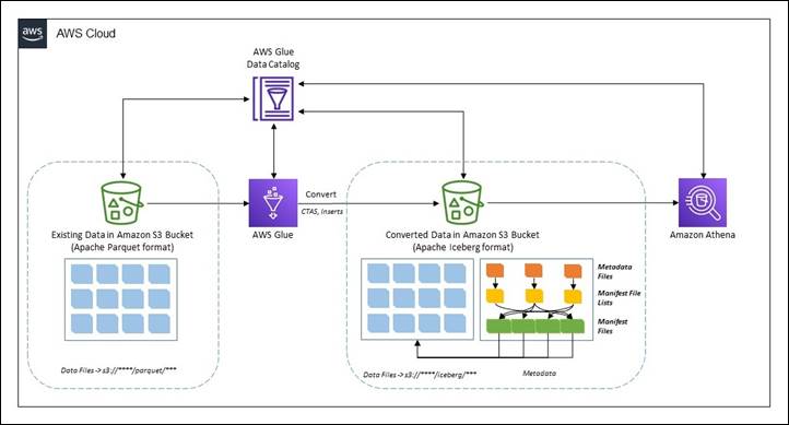
Migrate an existing data lake to a transactional data lake using Apache Iceberg

Post Syndicated from Rajdip Chaudhuri original https://aws.amazon.com/blogs/big-data/migrate-an-existing-data-lake-to-a-transactional-data-lake-using-apache-iceberg/

A data lake is a centralized repository that you can use to store all your structured and unstructured data at any scale. You can store your data as-is, without having to first structure the data and then run different types of analytics for better business insights. Over the years, data lakes on Amazon Simple Storage Service (Amazon S3) have become the default repository for enterprise data and are a common choice for a large set of users who query data for a variety of analytics and machine leaning use cases. Amazon S3 allows you to access diverse data sets, build business intelligence dashboards, and accelerate the consumption of data by adopting a modern data architecture or data mesh pattern on Amazon Web Services (AWS).

Analytics use cases on data lakes are always evolving. Oftentimes, you want to continuously ingest data from various sources into a data lake and query the data concurrently through multiple analytics tools with transactional capabilities. But traditionally, data lakes built on Amazon S3 are immutable and don’t provide the transactional capabilities needed to support changing use cases. With changing use cases, customers are looking for ways to not only move new or incremental data to data lakes as transactions, but also to convert existing data based on Apache Parquet to a transactional format. Open table formats, such as Apache Iceberg, provide a solution to this issue. Apache Iceberg enables transactions on data lakes and can simplify data storage, management, ingestion, and processing.

In this post, we show you how you can convert existing data in an Amazon S3 data lake in Apache Parquet format to Apache Iceberg format to support transactions on the data using Jupyter Notebook based interactive sessions over AWS Glue 4.0.

Existing Parquet to Iceberg migration

There are two broad methods to migrate the existing data in a data lake in Apache Parquet format to Apache Iceberg format to convert the data lake to a transactional table format.

In-place data upgrade

In an in-place data migration strategy, existing datasets are upgraded to Apache Iceberg format without first reprocessing or restating existing data. This means the data files in the data lake aren’t modified during the migration and all Apache Iceberg metadata files (manifests, manifest files, and table metadata files) are generated outside the purview of the data. In this method, the metadata are recreated in an isolated environment and colocated with the existing data files. This can be a much less expensive operation compared to rewriting all the data files. The existing data file format must be Apache Parquet, Apache ORC, or Apache Avro. An in-place migration can be performed in either of two ways:

  1. Using add_files: This procedure adds existing data files to an existing Iceberg table with a new snapshot that includes the files. Unlike migrate or snapshot, add_files can import files from a specific partition or partitions and doesn’t create a new Iceberg table. This procedure doesn’t analyze the schema of the files to determine if they match the schema of the Iceberg table. Upon completion, the Iceberg table treats these files as if they are part of the set of files owned by Apache Iceberg.
  2. Using migrate: This procedure replaces a table with an Apache Iceberg table loaded with the source’s data files. The table’s schema, partitioning, properties, and location are copied from the source table. Supported formats are Avro, Parquet, and ORC. By default, the original table is retained with the name table_BACKUP_. However, to leave the original table intact during the process, you must use snapshot to create a new temporary table that has the same source data files and schema.

In this post, we show you how you can use the Iceberg add_files procedure for an in-place data upgrade. Note that the migrate procedure isn’t supported in AWS Glue Data Catalog.

The following diagram shows a high-level representation.

CTAS migration of data

The create table as select (CTAS) migration approach is a technique where all the metadata information for Iceberg is generated along with restating all the data files. This method shadows the source dataset in batches. When the shadow is caught up, you can swap the shadowed dataset with the source.

The following diagram showcases the high-level flow.

Prerequisites

To follow along with the walkthrough, you must have the following:

You can check the data size using the following code in the AWS CLI or AWS CloudShell:

//Run this command to check the data size

aws s3 ls --summarize --human-readable --recursive s3://noaa-ghcn-pds/parquet/by_year/YEAR=2023

As of writing this post, there are 107 objects with total size of 70 MB for year 2023 in the Amazon S3 path.

Note that to implement the solution, you must complete a few preparatory steps.

Deploy resources using AWS CloudFormation

Complete the following steps to create the S3 bucket and the AWS IAM role and policy for the solution:

  1. Sign in to your AWS account and then choose Launch Stack to launch the CloudFormation template.

  1. For Stack name, enter a name.
  2. Leave the parameters at the default values. Note that if the default values are changed, then you must make corresponding changes throughout the following steps.
  3. Choose Next to create your stack.

This AWS CloudFormation template deploys the following resources:

  • An S3 bucket named demo-blog-post-XXXXXXXX (XXXXXXXX represents the AWS account ID used).
  • Two folders named parquet and iceberg under the bucket.
  • An IAM role and a policy named demoblogpostrole and demoblogpostscoped respectively.
  • An AWS Glue database named ghcn_db.
  • An AWS Glue Crawler named demopostcrawlerparquet.

After the the AWS CloudFormation template is successfully deployed:

  1. Copy the data in the created S3 bucket using following command in AWS CLI or AWS CloudShell. Replace XXXXXXXX appropriately in the target S3 bucket name.
    Note: In the example, we copy data only for the year 2023. However, you can work with the entire dataset, following the same instructions.

    aws s3 sync s3://noaa-ghcn-pds/parquet/by_year/YEAR=2023/ s3://demo-blog-post-XXXXXXXX/parquet/year=2023

  2. Open the AWS Management Console and go to the AWS Glue console.
  3. On the navigation pane, select Crawlers.
  4. Run the crawler named demopostcrawlerparquet.
  5. After the AWS Glue crawler demopostcrawlerparquet is successfully run, the metadata information of the Apache Parquet data will be cataloged under the ghcn_db AWS Glue database with the table name source_parquet. Notice that the table is partitioned over year and element columns (as in the S3 bucket).

  1. Use the following query to verify the data from the Amazon Athena console. If you’re using Amazon Athena for the first time in your AWS Account, set up a query result location in Amazon S3.
    SELECT * FROM ghcn_db.source_parquet limit 10;

Launch an AWS Glue Studio notebook for processing

For this post, we use an AWS Glue Studio notebook. Follow the steps in Getting started with notebooks in AWS Glue Studio to set up the notebook environment. Launch the notebooks hosted under this link and unzip them on a local workstation.

  1. Open AWS Glue Studio.
  2. Choose ETL Jobs.
  3. Choose Jupyter notebook and then choose Upload and edit an existing notebook. From Choose file, select required ipynb file and choose Open, then choose Create.
  4. On the Notebook setup page, for Job name, enter a logical name.
  5. For IAM role, select demoblogpostrole. Choose Create job. After a minute, the Jupyter notebook editor appears. Clear all the default cells.

The preceding steps launch an AWS Glue Studio notebook environment. Make sure you Save the notebook every time it’s used.

In-place data upgrade

In this section we show you how you can use the add_files procedure to achieve an in-place data upgrade. This section uses the ipynb file named demo-in-place-upgrade-addfiles.ipynb. To use with the add_files procedure, complete the following:

  1. On the Notebook setup page, for Job name, enter demo-in-place-upgrade for the notebook session as explained in Launch Glue notebook for processing.
  2. Run the cells under the section Glue session configurations. Provide the S3 bucket name from the prerequisites for the bucket_name variable by replacing XXXXXXXX.
  3. Run the subsequent cells in the notebook.

Notice that the cell under Execute add_files procedure section performs the metadata creation in the mentioned path.

Review the data file paths for the new Iceberg table. To show an Iceberg table’s current data files, .files can be used to get details such as file_path, partition, and others. Recreated files are pointing to the source path under Amazon S3.

Note the metadata file location after transformation. It’s pointing to the new folder named iceberg under Amazon S3. This can be checked using .snapshots to check Iceberg tables’ snapshot file location. Also, check the same in the Amazon S3 URI s3://demo-blog-post-XXXXXXXX/iceberg/ghcn_db.db/target_iceberg_add_files/metadata/. Also notice that there are two versions of the manifest list created after the add_files procedure has been run. The first is an empty table with the data schema and the second is adding the files.

The table is cataloged in AWS Glue under the database ghcn_db with the table type as ICEBERG.

Compare the count of records using Amazon Athena between the source and target table. They are the same.

In summary, you can use the add_files procedure to convert existing data files in Apache Parquet format in a data lake to Apache Iceberg format by adding the metadata files and without recreating the table from scratch. Following are some pros and cons of this method.

Pros

  • Avoids full table scans to read the data as there is no restatement. This can save time.
  • If there are any errors during while writing the metadata, only a metadata re-write is required and not the entire data.
  • Lineage of the existing jobs is maintained because the existing catalog still exists.

Cons

  • If data is processed (inserts, updates, and deletes) in the dataset during the metadata writing process, the process must be run again to include the new data.
  • There must be write downtime to avoid having to run the process a second time.
  • If a data restatement is required, this workflow will not work as source data files aren’t modified.

CTAS migration of data

This section uses the ipynb file named demo-ctas-upgrade.ipynb. Complete the following:

  1. On the Notebook setup page, for Job name, enter demo-ctas-upgrade for the notebook session as explained under Launch Glue notebook for processing.
  2. Run the cells under the section Glue session configurations. Provide the S3 bucket name from the prerequisites for the bucket_name variable by replacing XXXXXXXX.
  3. Run the subsequent cells in the notebook.

Notice that the cell under Create Iceberg table from Parquet section performs the shadow upgrade to Iceberg format. Note that Iceberg requires sorting the data according to table partitions before writing to the Iceberg table. Further details can be found in Writing Distribution Modes.

Notice the data and metadata file paths for the new Iceberg table. It’s pointing to the new path under Amazon S3. Also, check under the Amazon S3 URI s3://demo-blog-post-XXXXXXXX/iceberg/ghcn_db.db/target_iceberg_ctas/ used for this post.

The table is cataloged under AWS Glue under the database ghcn_db with the table type as ICEBERG.

Compare the count of records using Amazon Athena between the source and target table. They are same.

In summary, the CTAS method creates a new table by generating all the metadata files along with restating the actual data. Following are some pros and cons of this method:

Pros

  • It allows you to audit and validate the data during the process because data is restated.
  • If there are any runtime issues during the migration process, rollback and recovery can be easily performed by deleting the Apache Iceberg table.
  • You can test different configurations when migrating a source. You can create a new table for each configuration and evaluate the impact.
  • Shadow data is renamed to a different directory in the source (so it doesn’t collide with old Apache Parquet data).

Cons

  • Storage of the dataset is doubled during the process as both the original Apache Parquet and new Apache Iceberg tables are present during the migration and testing phase. This needs to be considered during cost estimation.
  • The migration can take much longer (depending on the volume of the data) because both data and metadata are written.
  • It’s difficult to keep tables in sync if there changes to the source table during the process.

Clean up

To avoid incurring future charges, and to clean up unused roles and policies, delete the resources you created: the datasets, CloudFormation stack, S3 bucket, AWS Glue job, AWS Glue database, and AWS Glue table.

Conclusion

In this post, you learned strategies for migrating existing Apache Parquet formatted data to Apache Iceberg in Amazon S3 to convert to a transactional data lake using interactive sessions in AWS Glue 4.0 to complete the processes. If you have an evolving use case where an existing data lake needs to be converted to a transactional data lake based on Apache Iceberg table format, follow the guidance in this post.

The path you choose for this upgrade, an in-place upgrade or CTAS migration, or a combination of both, will depend on careful analysis of the data architecture and data integration pipeline. Both pathways have pros and cons, as discussed. At a high level, this upgrade process should go through multiple well-defined phases to identify the patterns of data integration and use cases. Choosing the correct strategy will depend on your requirements—such as performance, cost, data freshness, acceptable downtime during migration, and so on.


About the author

Rajdip Chaudhuri is a Senior Solutions Architect with Amazon Web Services specializing in data and analytics. He enjoys working with AWS customers and partners on data and analytics requirements. In his spare time, he enjoys soccer and movies.

Network connectivity patterns for Amazon OpenSearch Serverless

Post Syndicated from Salman Ahmed original https://aws.amazon.com/blogs/big-data/network-connectivity-patterns-for-amazon-opensearch-serverless/

Amazon OpenSearch Serverless is an on-demand, auto-scaling configuration for Amazon OpenSearch Service. OpenSearch Serverless enables a broad set of use cases, such as real-time application monitoring, log analytics, and website search. OpenSearch Serverless lets you use OpenSearch without having to worry about scaling and managing an OpenSearch cluster. A collection can be accessed over the public internet or from your VPC. As you start accessing OpenSearch Serverless from different VPCs and accounts or from on premises, your connectivity patterns may change. In this post, we cover connectivity patterns and Domain Name System (DNS) resolution for your OpenSearch Serverless collection—whether accessed over the internet, within the VPC, within AWS, or from your on-premises location.

Foundational concepts

The following foundational concepts will help you better understand OpenSearch Serverless and DNS resolution.

Network access policy

The network access policy for OpenSearch Serverless determines whether the collection can be accessed over the internet or only through OpenSearch Serverless managed VPC endpoints. A single policy can be attached to multiple collections.

OpenSearch Serverless VPC endpoint

To access OpenSearch Serverless collections and dashboards privately from a VPC without using an internet gateway, you can create a VPC interface endpoint. When you create a VPC endpoint, it creates an elastic network interface (ENI) in each subnet that you enable for the VPC endpoint. These are requester-managed ENIs that serve as the entry point for traffic destined for the OpenSearch Serverless collection. When you create an OpenSearch Serverless VPC endpoint, the private DNS name option is enabled by default. This means that OpenSearch Serverless also creates an Amazon Route 53 private hosted zone and associates that with the VPC where the endpoint is created. This private hosted zone has a wildcard DNS record *.<region>.aoss.amazonaws.com pointing to the private DNS of the endpoint.

You create an OpenSearch Serverless VPC endpoint via the OpenSearch Serverless console or the OpenSearch Serverless API. You can’t create an OpenSearch Serverless VPC endpoint from the Amazon Virtual Private Cloud (Amazon VPC) console, although once created, you can see them on the VPC console as well.

Amazon Route 53 Resolver

Let’s understand what Amazon Route 53 Resolver does when an Amazon Elastic Compute Cloud (Amazon EC2) instance queries a DNS name. DNS queries originating from the VPC go to the Route 53 Resolver at the VPC+2 IP address. When a DNS query reaches the resolver, it checks if there are any Route 53 forward rules. If it matches, then it forwards the query to the DNS server provided by that rule. If the query remains unresolved, Route 53 Resolver proceeds to check the private hosted zones associated with the originating VPC. If it still remains unresolved, then it checks for VPC DNS, which helps to resolve EC2 DNS names. Lastly, if the query still isn’t resolved, Route 53 Resolver checks the public DNS. The following diagram illustrates this order or operations.

Route 53 DNS Overview

Route 53 Resolver inbound endpoints

Workloads utilizing resources both in a VPC and on premises need to resolve DNS records hosted on-premises and resources hosted in the VPC. With Route 53 Resolver inbound endpoints, you can resolve DNS queries to your VPC from your on-premises network or another VPC.

In the following sections, we provide an overview of connectivity patterns and DNS resolution.

Access an OpenSearch Serverless collection from Amazon EC2 (via internet gateway)

The following figure demonstrates the connectivity pattern to access an OpenSearch Serverless collection over the internet. The collection has an access type set to public, which allows authorized users to connect to the collection over the internet. An EC2 instance within the VPC can establish a connection to the collection via the internet gateway, and users outside the VPC can also access this collection over the internet.

Access an OpenSearch Serverless collection from Amazon EC2 (via internet gateway)

The workflow has the following steps, as indicated in the preceding diagram:

A. The EC2 instance performs a DNS lookup to Route 53 Resolver at a VPC+2 IP address. Route 53 Resolver returns the public IP addresses of the OpenSearch Serverless collection.

B. The EC2 instance sends a data request via an internet gateway to the OpenSearch Serverless collection using this public IP address.

C. An external client resolves to the public IP addresses of the OpenSearch Serverless collection and reaches it via the internet.

Now let’s perform a dig command for the collection or dashboard URL from the EC2 instance, and we observe that it’s resolving to a public IP address.

The following command uses an OpenSearch Serverless collection:

sh-5.2$ dig +short <collection-id>.<region>.aoss.amazonaws.com
192.0.2.10
198.51.100.204
192.0.2.45
198.51.100.55
192.0.2.100
203.0.113.66

The following command uses an OpenSearch dashboard:

sh-5.2$ dig +short dashboards.<region>.aoss.amazonaws.com
192.0.2.10
198.51.100.204
192.0.2.45
198.51.100.55
192.0.2.100
203.0.113.66

Now that you have implemented an OpenSearch Serverless collection with a network access policy as public, you can make the same collection accessible privately within the VPC. To achieve this, complete the following steps:

  1. Modify the network access policy of the collection and change the access type to VPC.
  2. Select the option Create VPC endpoints.

Access type for OpenSearch Serverless

  1. Choose the VPC and at least two subnets where you would like to have a VPC endpoint ENI for high availability.
  2. Choose Confirm to create the VPC endpoint.

Create VPC endpoints for Amazon OpenSearch Serverless

  1. Lastly, select the VPC endpoint and update the policy.

Access Type VPC Endpoint for Amazon OpenSearch Serverless

With the creation of the VPC endpoint, a Route 53 private hosted zone is also created within your account and associated with your VPC. In this setup, a CNAME record *.us-east-1.aoss.amazonaws.com is created to direct to the Regional AWS PrivateLink endpoint, as depicted in the following screenshot.

Route 53 Private Hosted Zone

Due to the private hosted zone associated with the VPC, Route 53 Resolver gives preference to the private hosted zone to resolve any DNS query originating from the VPC. DNS requests for the OpenSearch Serverless collection originating from the EC2 instance get resolved using this associated private hosted zone and resolve to the private IP addresses of the VPC endpoint, which allows Amazon EC2 to connect to the serverless collection via VPC endpoints vs. the internet gateway. We expand on this in the following section.

Access an OpenSearch Serverless collection from Amazon EC2 (via interface VPC endpoints)

The following figure demonstrates the connectivity pattern to access an OpenSearch Serverless collection privately from the VPC. The collection has an access type set to VPC endpoint, restricting access solely from the resources within the VPC via the VPC endpoint and preventing external users from connecting. With the creation of the VPC endpoint, a private hosted zone is also associated with this VPC. An EC2 instance within the VPC can establish a connection with the collection using the VPC endpoint, but resources outside of the VPC don’t have access to this collection because of the network access policy.

Access an OpenSearch Serverless collection from Amazon EC2 (via interface VPC endpoints)

The workflow consists of the following steps:

A. The EC2 instance performs a DNS lookup to Route 53 Resolver at a VPC+2 IP address. Route 53 Resolver returns the private IP addresses of the VPC endpoint because there is a private hosted zone associated with the VPC containing a CNAME record.

B. The EC2 instance sends a data request via the VPC interface endpoint to the OpenSearch Serverless collection.

C. An external client resolves to the public IP addresses of the OpenSearch Serverless collection but is unable to reach it because the network policy restricts to the VPC.

Now let’s perform a dig command for the collection or dashboard URL from the EC2 instance, and we observe that it’s resolving to the private IP addresses belonging to the VPC endpoints.

Use the following code for an OpenSearch Serverless collection:

sh-5.2$ dig +short <collection-id>.<region>.aoss.amazonaws.com
10.0.1.98
10.0.2.83

Use the following code for an OpenSearch dashboard:

sh-5.2$ dig +short dashboards.<region>.aoss.amazonaws.com
10.0.1.98
10.0.2.83

Access an OpenSearch Serverless collection from many VPCs (via interface VPC endpoints) with a VPC endpoint in each VPC

The following figure demonstrates the connectivity pattern to use the same VPC endpoint to connect to multiple OpenSearch Serverless collections. In this scenario, a VPC endpoint is created in each VPC to enable EC2 instances within the VPCs to utilize the VPC endpoint as the connectivity path to OpenSearch Serverless. A private hosted zone is auto generated for each endpoint and associated with the corresponding VPC. Network policies of OpenSearch Serverless collections are updated to allow both VPC Endpoint-1 and VPC Endpoint-2, which allows the EC2 instance in VPC-1 to access both collections via VPC Endpoint-1 and EC2 instances in VPC-2 to access both collections via VPC Endpoint-2.

Access an OpenSearch Serverless collection from many VPCs (via interface VPC endpoints) with a VPC endpoint in each VPC

The workflow consists of the following steps:

A. The EC2 instance performs a DNS lookup to Route 53 Resolver at a VPC+2 IP address. Route 53 Resolver returns the private IP addresses of the VPC endpoint (the EC2 instance in VPC-1 gets the IP address of VPC Endpoint-1 and the EC2 instance in VPC-2 gets the IP address of VPC Endpoint-2), because there is a private hosted zone associated with each of the VPCs containing a CNAME record.

B. The EC2 instance sends a data request via the VPC interface endpoint to the OpenSearch Serverless collection.

Access an OpenSearch Serverless collection from many VPCs (via interface VPC endpoints) with a VPC endpoint in a centralized VPC

In the previous connectivity pattern, we had one endpoint in each VPC through which VPC resources accessed OpenSearch Serverless collections. Many organizations would like to maintain control of these endpoints and keep these in a centralized VPC.

The following figure demonstrates the connectivity pattern to use a centralized VPC endpoint to connect to multiple OpenSearch Serverless collections from multiple VPCs. In this scenario, a VPC interface endpoint is created in a centralized VPC. A private hosted zone is auto generated for this VPC endpoint and associated with the centralized VPC, and then manually associated with VPC-1 and VPC-2. The DNS query for OpenSearch Serverless collections from VPC-1 and VPC-2 gets resolved to the centralized VPC endpoint due to the private hosted zone association. Network policies for both collections allow access from the centralized VPC endpoint only. All three VPCs (centralized, VPC-1, and VPC-2) are connected via AWS Transit Gateway and route tables have routes to direct traffic between VPC-1 and VPC-2 to the centralized VPC and vice versa.

Access an OpenSearch Serverless collection from many VPCs (via interface VPC endpoints) with a VPC endpoint in a centralized VPC

The workflow consists of the following steps:

A. The EC2 instance performs a DNS lookup to Route 53 Resolver at a VPC+2 IP address. Route 53 Resolver returns the private IP addresses of the centralized VPC endpoint, because there is a private hosted zone associated with each VPC containing a CNAME record.

B. The EC2 instance sends a data request to the Transit Gateway ENI in its own VPC. The Transit Gateway route table is checked and the data request is forwarded to the Transit Gateway ENI in the centralized VPC. The Transit Gateway ENI in the centralized VPC sends it to the OpenSearch Serverless collection via the VPC interface endpoint.

Access an OpenSearch Serverless collection from on premises (via AWS Site-to-Site VPN or AWS Direct Connect)

The following figure demonstrates the connectivity pattern for accessing OpenSearch Serverless collections from on premises. You can use either AWS Direct Connect or AWS Site-to-Site VPN to establish connectivity between on-premises and AWS resources. In the following example, Direct Connect is used for the connectivity between AWS and on premises. An OpenSearch Serverless VPC endpoint is created in the VPC, and a private hosted zone is automatically generated and associated with this VPC. The network policy of the OpenSearch Serverless collection is updated to allow connectivity only from the VPC endpoint.

To access these OpenSearch Serverless collections privately from the on-premises environment, resources need to resolve the OpenSearch Serverless collection DNS to the OpenSearch Serverless VPC endpoint IP address. By default, OpenSearch Serverless DNS resolves to the public IP addresses and attempts to access OpenSearch Serverless via the internet. To ensure that OpenSearch Serverless is accessed via the VPC endpoint from on premises, you need to ensure that DNS queries are resolved to a VPC endpoint’s private IP address. Resources inside the VPC use Route 53 Resolver, available at a VPC+2 IP address, to resolve these queries to the VPC endpoint. Route 53 Resolver checks the associated private hosted zone to resolve the query to the VPC endpoint. However, the VPC+2 IP address is not accessible from on premises. To address this, you can utilize the Route 53 Resolver inbound endpoint.

To achieve this, you can create an inbound endpoint in your VPC by following the steps outlined in Configuring inbound forwarding, and then update the on-premises DNS server to forward all the DNS requests for *.<region>.aoss.amazonaws.com to the IP address of the Route 53 Resolver inbound endpoint. When the on-premises client obtains the IP address of the VPC endpoint, it can use Direct Connect or Site-to-Site VPN to establish a private connection to the OpenSearch Serverless collection.

Access an OpenSearch Serverless collection from on premises (via AWS Site-to-Site VPN or AWS Direct Connect)

The workflow contains the following steps:

A. The on-premises client sends a DNS lookup to the on-premises DNS resolver. The on-premises DNS resolver forwards this request to the Route 53 Resolver inbound endpoint. The Route 53 Resolver inbound endpoint sends a DNS lookup to Route 53 Resolver at a VPC+2 IP address. Route 53 Resolver returns the private IP addresses of the VPC endpoint, because there is a private hosted zone associated with this VPC containing a CNAME record.

B. The on-premises client sends a data request to the OpenSearch Serverless collection, which routes via Direct Connect or Site-to-site VPN to the VPC interface endpoint and finally to the OpenSearch Serverless collection.

Conclusion

In this post, we showed you various connectivity patterns for OpenSearch Serverless. We covered the use of hybrid DNS and using a Route 53 Resolver inbound endpoint to allow connectivity from on premises for OpenSearch Serverless. You can choose from various centralization models for reaching multiple OpenSearch Serverless collections within the AWS Cloud or from on-premises locations. Get started today by connecting to OpenSearch Serverless from the various network patterns we discussed.


About the authors

Salman AhmedSalman Ahmed is a Sr. Technical Account Manager in AWS Enterprise Support. He enjoys working with Enterprise Support customers to help them with design, implementation and supporting cloud infrastructure. He also has a passion for networking services and with 12+ years of experience, he leverages that to help customers with adoption of AWS Transit Gateway, AWS Direct Connect and various other AWS networking services.

Ankush GoyalAnkush Goyal is Enterprise Support Lead in AWS Enterprise Support who helps enterprise support customers streamline their cloud operations on AWS. He is a results-driven IT professional with over 18 years of experience.

Rohit AswaniRohit Aswani is a Senior Specialist Solutions Architect focussed on Networking at AWS, where he helps customers build and design scalable, highly-available, secure, resilient and cost effective networks. He holds a MS in Telecommunication Systems Management from Northeastern University, specializing in Computer Networking. In his spare time, Rohit enjoys hiking, traveling and exploring new coffee places.

Use the new SQL commands MERGE and QUALIFY to implement and validate change data capture in Amazon Redshift

Post Syndicated from Yanzhu Ji original https://aws.amazon.com/blogs/big-data/use-the-new-sql-commands-merge-and-qualify-to-implement-and-validate-change-data-capture-in-amazon-redshift/

Amazon Redshift is a fully managed, petabyte-scale data warehouse service in the cloud. Tens of thousands of customers use Amazon Redshift to process exabytes of data every day to power their analytics workloads.

Amazon Redshift has added many features to enhance analytical processing like ROLLUP, CUBE and GROUPING SETS, which were demonstrated in the post Simplify Online Analytical Processing (OLAP) queries in Amazon Redshift using new SQL constructs such as ROLLUP, CUBE, and GROUPING SETS. Amazon Redshift has recently added many SQL commands and expressions. In this post, we talk about two new SQL features, the MERGE command and QUALIFY clause, which simplify data ingestion and data filtering.

One familiar task in most downstream applications is change data capture (CDC) and applying it to its target tables. This task requires examining the source data to determine if it is an update or an insert to existing target data. Without the MERGE command, you needed to test the new dataset against the existing dataset using a business key. When that didn’t match, you inserted new rows in the existing dataset; otherwise, you updated existing dataset rows with new dataset values.

The MERGE command conditionally merges rows from a source table into a target table. Traditionally, this could only be achieved by using multiple insert, update, or delete statements separately. When using multiple statements to update or insert data, there is a risk of inconsistencies between the different operations. Merge operation reduces this risk by ensuring that all operations are performed together in a single transaction.

The QUALIFY clause filters the results of a previously computed window function according to user‑specified search conditions. You can use the clause to apply filtering conditions to the result of a window function without using a subquery. This is similar to the HAVING clause, which applies a condition to further filter rows from a WHERE clause. The difference between QUALIFY and HAVING is that filtered results from the QUALIFY clause could be based on the result of running window functions on the data. You can use both the QUALIFY and HAVING clauses in one query.

In this post, we demonstrate how to use the MERGE command to implement CDC and how to use QUALIFY to simplify validation of those changes.

Solution overview

In this use case, we have a data warehouse, in which we have a customer dimension table that needs to always get the latest data from the source system. This data must also reflect the initial creation time and last update time for auditing and tracking purposes.

A simple way to solve this is to override the customer dimension fully every day; however, that won’t achieve the update tracking, which is an audit mandate, and it might not be feasible to do for bigger tables.

You can load sample data from Amazon S3 by following the instruction here. Using the existing customer table under sample_data_dev.tpcds, we create a customer dimension table and a source table that will contain both updates for existing customers and inserts for new customers. We use the MERGE command to merge the source table data with the target table (customer dimension). We also show how to use the QUALIFY clause to simplify validating the changes in the target table.

To follow along with the steps in this post, we recommend downloading the accompanying notebook, which contains all the scripts to run for this post. To learn about authoring and running notebooks, refer to Authoring and running notebooks.

Prerequisites

You should have the following prerequisites:

Create and populate the dimension table

We use the existing customer table under sample_data_dev.tpcds to create a customer_dimension table. Complete the following steps:

  1. Create a table using a few selected fields, including the business key, and add a couple of maintenance fields for insert and update timestamps:
     -- create the customer dimension table DROP TABLE IF EXISTS customer_dim CASCADE;
    CREATE TABLE customer_dim ( 
    customer_dim_id     bigint GENERATED BY DEFAULT AS IDENTITY(1, 1), 
    c_customer_sk integer NOT NULL ENCODE az64 distkey,
    c_first_name character(20) ENCODE lzo,
    c_last_name character(30) ENCODE lzo,
    c_current_addr_sk integer ENCODE az64,
    c_birth_country character varying(20) ENCODE lzo,
    c_email_address character(50) ENCODE lzo,
    record_insert_ts    timestamp WITHOUT time ZONE DEFAULT current_timestamp ,
    record_upd_ts       timestamp WITHOUT time ZONE DEFAULT NULL
    )
    SORTKEY (c_customer_sk);

  2. Populate the dimension table:
    -- populate dimension 
    insert into customer_dim 
           (c_customer_sk, c_first_name,c_last_name, c_current_addr_sk, c_birth_country, c_email_address) 
    select  c_customer_sk, c_first_name,c_last_name, c_current_addr_sk, c_birth_country, c_email_address
    from “sample_data_dev”.”tpcds”.”customer”;

  3. Validate the row count and the contents of the table:
    -- check customers count and look at sample data
    select count(1) from customer_dim; 
    select * from customer_dim limit 10;

Simulate customer table changes

Use the following code to simulate changes made to the table:

-- create a source table with some updates and some inserts
-- Update- Email has changed for 100 customers 
drop table if exists src_customer;
create table src_customer distkey(c_customer_sk) as 
select c_customer_sk , c_first_name , c_last_name, c_current_addr_sk, c_birth_country, ‘x’+c_email_address as c_email_address, getdate() as effective_dt
from   customer_dim 
where  c_email_address is not null
limit 100;


-- also let’s add three completely new customers
insert into src_customer values 
(15000001, ‘Customer#15’,’000001’, 10001 ,’USA’    , ‘Customer#[email protected]’, getdate() ),
(15000002, ‘Customer#15’,’000002’, 10002 ,’MEXICO’ , ‘Customer#[email protected]’, getdate() ),
(15000003, ‘Customer#15’,’000003’, 10003 ,’CANADA’ , ‘Customer#[email protected]’, getdate() );

-- check source count
select count(1) from src_customer;

Merge the source table into the target table

Now you have a source table with some changes you need to merge with the customer dimension table.

Before the MERGE command, this type of task needed two separate UPDATE and INSERT commands to implement:

-- merge changes to dim customer
BEGIN TRANSACTION;
-- update current records
UPDATE customer_dim
SET    c_first_name      = src.c_first_name      ,
       c_last_name       = src.c_last_name       , 
       c_current_addr_sk = src.c_current_addr_sk , 
       c_birth_country   = src.c_birth_country   , 
       c_email_address   = src.c_email_address   ,
       record_upd_ts     = current_timestamp
from   src_customer AS src
where  customer_dim.c_customer_sk = src.c_customer_sk ;
-- Insert new records
INSERT INTO customer_dim (c_customer_sk, c_first_name,c_last_name, c_current_addr_sk, c_birth_country, c_email_address) 
select src.c_customer_sk, src.c_first_name,src.c_last_name, src.c_current_addr_sk, src.c_birth_country, src.c_email_address 
from   src_customer AS src
where  src.c_customer_sk NOT IN (select c_customer_sk from customer_dim);
-- end merge operation
COMMIT TRANSACTION;

The MERGE command uses a more straightforward syntax, in which we use the key comparison result to decide if we perform an update DML operation (when matched) or an insert DML operation (when not matched):

MERGE INTO customer_dim using src_customer AS src ON customer_dim.c_customer_sk = src.c_customer_sk
WHEN MATCHED THEN UPDATE 
SET c_first_name      = src.c_first_name      ,
    c_last_name       = src.c_last_name       , 
    c_current_addr_sk = src.c_current_addr_sk , 
    c_birth_country   = src.c_birth_country   , 
    c_email_address   = src.c_email_address   ,
    record_upd_ts     = current_timestamp
WHEN NOT MATCHED THEN INSERT (c_customer_sk, c_first_name,c_last_name, c_current_addr_sk, c_birth_country, c_email_address) 
                      VALUES (src.c_customer_sk, src.c_first_name,src.c_last_name, src.c_current_addr_sk, src.c_birth_country, src.c_email_address );

Validate the data changes in the target table

Now we need to validate the data has made it correctly to the target table. We can first check the updated data using the update timestamp. Because this was our first update, we can examine all rows where the update timestamp is not null:

-- Check the changes
-- to get updates
select * 
from customer_dim
where record_upd_ts is not null

Use QUALIFY to simplify validation of the data changes

We need to examine the data inserted in this table most recently. One way to do that is to rank the data by its insert timestamp and get those with the first rank. This requires using the window function rank() and also requires a subquery to get the results.

Before the availability of QUALIFY, we needed to build that using a subquery like the following:

select customer_dim_id,c_customer_sk ,c_first_name ,c_last_name ,c_current_addr_sk,c_birth_country ,c_email_address ,record_insert_ts ,record_upd_ts 
from 
( select rank() OVER (ORDER BY DATE_TRUNC(‘second’,record_insert_ts) desc) AS rnk, 
         customer_dim_id,c_customer_sk ,c_first_name ,c_last_name ,c_current_addr_sk,c_birth_country ,c_email_address ,record_insert_ts ,record_upd_ts 
  from customer_dim
  where record_upd_ts is null)
where rnk = 1;

The QUALIFY function eliminates the need for the subquery, as in the following code snippet:

-- to get the newly inserted rows we can make use of Qualify feature
select * 
from customer_dim
where record_upd_ts is null
qualify rank() OVER (ORDER BY DATE_TRUNC(‘second’,record_insert_ts) desc) = 1 

Validate all data changes

We can union the results of both queries to get all the inserts and update changes:

-- To get all changes
select *
from (
select 'Updates' as operations, cd.* 
from   customer_dim as cd
where  cd.record_upd_ts is not null
union 
select 'Inserts' as operations, cd.* 
from customer_dim cd
where cd.record_upd_ts is null
qualify rank() OVER (ORDER BY DATE_TRUNC('second',cd.record_insert_ts) desc) = 1 
) order by 1

Clean up

To clean up the resources used in the post, delete the Redshift provisioned cluster or Redshift Serverless workgroup and namespace you created for this post (this will also drop all the objects created).

If you used an existing Redshift provisioned cluster or Redshift Serverless workgroup and namespace, use the following code to drop these objects:

DROP TABLE IF EXISTS customer_dim CASCADE;
DROP TABLE IF EXISTS src_customer CASCADE;

Conclusion

When using multiple statements to update or insert data, there is a risk of inconsistencies between the different operations. The MERGE operation reduces this risk by ensuring that all operations are performed together in a single transaction. For Amazon Redshift customers who are migrating from other data warehouse systems or who regularly need to ingest fast-changing data into their Redshift warehouse, the MERGE command is a straightforward way to conditionally insert, update, and delete data from target tables based on existing and new source data.

In most analytic queries that use window functions, you may need to use those window functions in your WHERE clause as well. However, this is not permitted, and to do so, you have to build a subquery that contains the required window function and then use the results in the parent query in the WHERE clause. Using the QUALIFY clause eliminates the need for a subquery and therefore simplifies the SQL statement and makes it less difficult to write and read.

We encourage you to start using those new features and give us your feedback. For more details, refer to MERGE and QUALIFY clause.


About the authors

Yanzhu Ji is a Product Manager in the Amazon Redshift team. She has experience in product vision and strategy in industry-leading data products and platforms. She has outstanding skill in building substantial software products using web development, system design, database, and distributed programming techniques. In her personal life, Yanzhu likes painting, photography, and playing tennis.

Ahmed Shehata is a Senior Analytics Specialist Solutions Architect at AWS based on Toronto. He has more than two decades of experience helping customers modernize their data platforms. Ahmed is passionate about helping customers build efficient, performant, and scalable analytic solutions.

Ranjan Burman is an Analytics Specialist Solutions Architect at AWS. He specializes in Amazon Redshift and helps customers build scalable analytical solutions. He has more than 16 years of experience in different database and data warehousing technologies. He is passionate about automating and solving customer problems with cloud solutions.