Tag Archives: Advanced (300)

Externalize Amazon MSK Connect configurations with Terraform

Post Syndicated from Ramc Venkatasamy original https://aws.amazon.com/blogs/big-data/externalize-amazon-msk-connect-configurations-with-terraform/

Managing configurations for Amazon MSK Connect, a feature of Amazon Managed Streaming for Apache Kafka (Amazon MSK), can become challenging, especially as the number of topics and configurations grows. In this post, we address this complexity by using Terraform to optimize the configuration of the Kafka topic to Amazon S3 Sink connector. By adopting this strategic approach, you can establish a robust and automated mechanism for handling MSK Connect configurations, eliminating the need for manual intervention or connector restarts. This efficient solution will save time, reduce errors, and provide better control over your Kafka data streaming processes. Let’s explore how Terraform can simplify and enhance the management of MSK Connect configurations for seamless integration with your infrastructure.

Solution overview

At a well-known AWS customer, the management of their constantly growing MSK Connect S3 Sink connector topics has become a significant challenge. The challenges lie in the overhead of managing configurations, as well as dealing with patching and upgrades. Manually handling Kubernetes (K8s) configs and restarting connectors can be cumbersome and error-prone, making it difficult to keep track of changes and updates. At the time of writing this post, MSK Connect does not offer native mechanisms to easily externalize the Kafka topic to S3 Sink configuration.

To address these challenges, we introduce Terraform, an infrastructure as code (IaC) tool. Terraform’s declarative approach and extensive ecosystem make it an ideal choice for managing MSK Connect configurations.

By externalizing Kafka topic to S3 configurations, organizations can achieve the following:

  • Scalability – Effortlessly manage a growing number of topics, ensuring the system can handle increasing data volumes without difficulty
  • Flexibility – Seamlessly integrate MSK Connect configurations with other infrastructure components and services, enabling adaptability to changing business needs
  • Automation – Automate the deployment and management of MSK Connect configurations, reducing manual intervention and streamlining operational tasks
  • Centralized management – Achieve improved governance with centralized management, version control, auditing, and change tracking, ensuring better control and visibility over the configurations

In the following sections, we provide a detailed guide on establishing Terraform for MSK Connect configuration management, defining and decentralizing Topic configurations, and deploying and updating configurations using Terraform.

Prerequisites

Before proceeding with the solution, ensure you have the following resources and access:

  • You need access to an AWS account with sufficient permissions to create and manage resources, including AWS Identity and Access Management (IAM) roles and MSK clusters.
  • To simplify the setup, use the provided AWS CloudFormation template. This template will create the necessary MSK cluster and required resources for this post.
  • For this post, we are using the latest Terraform version (1.5.6).

By ensuring you have these prerequisites in place, you will be ready to follow the instructions and streamline your MSK Connect configurations with Terraform. Let’s get started!

Setup

Setting up Terraform for MSK Connect configuration management includes the following:

  • Installation of Terraform and setting up the environment
  • Setting up the necessary authentication and permissions

Defining and decentralizing topic configurations using Terraform includes the following:

  • Understanding the structure of Terraform configuration files
  • Determining the required variables and resources
  • Utilizing Terraform’s modules and interpolation for flexibility

The decision to externalize the configuration was primarily driven by the customer’s business requirement. They anticipated the need to add topics periodically and wanted to avoid the need to bring down and write specific code each time. Given the limitations of MSK Connect (as of this writing), it’s important to note that MSK Connect can handle up to 300 workers. For this proof of concept (POC), we opted for a configuration with 100 topics directed to a single Amazon Simple Storage Service (Amazon S3) bucket. To ensure compatibility within the 300-worker limit, we set the MCU count to 1 and configured auto scaling with a maximum of 2 workers. This ensures that the configuration remains within the bounds of the 300-worker maximum.

To make the configuration more flexible, we specify the variables that can be utilized in the code.(variables.tf):

variable "aws_region" {
description = "The AWS region to deploy resources in."
type = string
}

variable "s3_bucket_name" {
description = "s3_bucket_name."
type = string
}

variable "topics" {
description = "topics"
type = string
}

variable "msk_connect_name" {
description = "Name of the MSK Connect instance."
type = string
}

variable "msk_connect_description" {
description = "Description of the MSK Connect instance."
type = string
}

# Rest of the variables...

To set up the AWS MSK Connector for the S3 Sink, we need to provide various configurations. Let’s examine the connector_configuration block in the code snippet provided in the main.tf file in more detail:

connector_configuration = {
"connector.class" = "io.confluent.connect.s3.S3SinkConnector"
"s3.region" = "us-east-1"
"flush.size" = "5"
"schema.compatibility" = "NONE"
"tasks.max" = "1"
"topics" = var.topics
"format.class" = "io.confluent.connect.s3.format.json.JsonFormat"
"partitioner.class" = "io.confluent.connect.storage.partitioner.DefaultPartitioner"
"value.converter.schemas.enable" = "false"
"value.converter" = "org.apache.kafka.connect.json.JsonConverter"
"storage.class" = "io.confluent.connect.s3.storage.S3Storage"
"key.converter" = "org.apache.kafka.connect.storage.StringConverter"
"s3.bucket.name" = var.s3_bucket_name
"topics.dir" = "cxdl-data/KairosTelemetry"
}

The kafka_cluster block in the code snippet defines the Kafka cluster details, including the bootstrap servers and VPC settings. You can reference the variables to specify the appropriate values:

kafka_cluster {
apache_kafka_cluster {
bootstrap_servers = var.bootstrap_servers

vpc {
security_groups = [var.security_groups]
subnets = [var.aws_subnet_example1_id, var.aws_subnet_example2_id, var.aws_subnet_example3_id]
}
}
}

To secure the connection between Kafka and the connector, the code snippet includes configurations for authentication and encryption:

  • The kafka_cluster_client_authentication block sets the authentication type to IAM, enabling the use of IAM for authentication
  • The kafka_cluster_encryption_in_transit block enables TLS encryption for data transfer between Kafka and the connector
  kafka_cluster_client_authentication {
    authentication_type = "IAM"
  }

  kafka_cluster_encryption_in_transit {
    encryption_type = "TLS"
  }

You can externalize the variables and provide dynamic values using a var.tfvars file. Let’s assume the content of the var.tfvars file is as follows:

aws_region = "us-east-1"
msk_connect_name = "confluentinc-MSK-connect-s3-2"
msk_connect_description = "My MSK Connect instance"
s3_bucket_name = "msk-lab-xxxxxxxxxxxx-target-bucket"
topics = "salesdb.salesdb.CUSTOMER,salesdb.salesdb.CUSTOMER_SITE,salesdb.salesdb.PRODUCT,salesdb.salesdb.PRODUCT_CATEGORY,salesdb.salesdb.SALES_ORDER,salesdb.salesdb.SALES_ORDER_ALL,salesdb.salesdb.SALES_ORDER_DETAIL,salesdb.salesdb.SALES_ORDER_DETAIL_DS,salesdb.salesdb.SUPPLIER"
bootstrap_servers = "b-2.mskclustermskconnectl.4xwlfx.c11.kafka.us-east-1.amazonaws.com:9098,b-3.mskclustermskconnectl.4xwlfx.c11.kafka.us-east-1.amazonaws.com:9098,b-1.mskclustermskconnectl.4xwlfx.c11.kafka.us-east-1.amazonaws.com:9098“
aws_subnet_example1_id = "subnet-016ef7bb5f5db5759"
aws_subnet_example2_id = "subnet-0114c390d379134fa"
aws_subnet_example3_id = "subnet-0f6352ad89a1454f2"
security_groups = "sg-07eb8f8e4559334e7"
aws_mskconnect_custom_plugin_example_arn = "arn:aws:kafkaconnect:us-east-1:xxxxxxxxxxxx:custom-plugin/confluentinc-kafka-connect-s3-10-0-3/e9aeb52e-d172-4dba-9de5-f5cf73f1cb9e-2"
aws_mskconnect_custom_plugin_example_latest_revision = "1"
aws_iam_role_example_arn = "arn:aws:iam::xxxxxxxxxxxx:role/msk-connect-lab-S3ConnectorIAMRole-3LBTU7YAV9CM"

Deploy and update configurations using Terraform

Once you’ve defined your MSK Connect infrastructure using Terraform, applying these configurations is a straightforward process for creating or updating your infrastructure. This becomes particularly convenient when a new topic needs to be added. Thanks to the externalized configuration, incorporating this change is now a seamless task. The steps are as follows:

  1. Download and install Terraform from the official website (https://www.terraform.io/downloads.html) for your operating system.
  2. Confirm the installation by running the terraform version command on your command line interface.
  3. Ensure that you have configured your AWS credentials using the AWS Command Line Interface (AWS CLI) or by setting environment variables. You can use the aws configure command to configure your credentials if you’re using the AWS CLI.
  4. Place the main.tf, variables.tf, and var.tfvars files in the same Terraform directory.
  5. Open a command line interface, navigate to the directory containing the Terraform files, and run the command terraform init to initialize Terraform and download the required providers.
  6. Run the command terraform plan -var-file="var.tfvars" to review the run plan.

This command shows the changes that Terraform will make to the infrastructure based on the provided variables. This step is optional but is often used as a preview of the changes Terraform will make.

  1. If the plan looks correct, run the command terraform apply -var-file="var.tfvars" to apply the configuration.

Terraform will create the MSK_Connect in your AWS account. This will prompt you for confirmation before proceeding.

  1. After the terraform apply command is complete, verify the infrastructure has been created or updated on the console.
  2. For any changes or updates, modify your Terraform files (main.tf, variables.tf, var.tfvars) as needed, and then rerun the terraform plan and terraform apply commands.
  3. When you no longer need the infrastructure, you can use terraform destroy -var-file="var.tfvars" to remove all resources created by your Terraform files.

Be careful with this command because it will delete all the resources defined in your Terraform files.

Conclusion

In this post, we addressed the challenges faced by a customer in managing MSK Connect configurations and described a Terraform-based solution. By externalizing Kafka topic to Amazon S3 configurations, you can streamline your configuration management processes, achieve scalability, enhance flexibility, automate deployments, and centralize management. We encourage you to use Terraform to optimize your MSK Connect configurations and explore further possibilities in managing your streaming data pipelines efficiently.

To get started with externalizing MSK Connect configurations using Terraform, refer to the provided implementation steps and the Getting Started with Terraform guide, MSK Connect documentation, Terraform documentation, and example GitHub repository.

Using Terraform to externalize the Kafka topic to Amazon S3 Sink configuration in MSK Connect offers a powerful solution for managing and scaling your streaming data pipelines. By automating the deployment, updating, and central management of configurations, you can ensure efficiency, flexibility, and scalability in your data processing workflows.


About the Author

RamC Venkatasamy is a Solutions Architect based in Bloomington, Illinois. He helps AWS Strategic customers transform their businesses in the cloud. With a fervent enthusiasm for Serverless, Event-Driven Architecture and GenAI.
How Chime Financial uses AWS to build a serverless stream analytics platform and defeat fraudsters

Post Syndicated from Khandu Shinde original https://aws.amazon.com/blogs/big-data/how-chime-financial-uses-aws-to-build-a-serverless-stream-analytics-platform-and-defeat-fraudsters/

This is a guest post by Khandu Shinde, Staff Software Engineer and Edward Paget, Senior Software Engineering at Chime Financial.

Chime is a financial technology company founded on the premise that basic banking services should be helpful, easy, and free. Chime partners with national banks to design member first financial products. This creates a more competitive market with better, lower-cost options for everyday Americans who aren’t being served well by traditional banks. We help drive innovation, inclusion, and access across the industry.

Chime has a responsibility to protect our members against unauthorized transactions on their accounts. Chime’s Risk Analysis team constantly monitors trends in our data to find patterns that indicate fraudulent transactions.

This post discusses how Chime utilizes AWS Glue, Amazon Kinesis, Amazon DynamoDB, and Amazon SageMaker to build an online, serverless fraud detection solution — the Chime Streaming 2.0 system.

Problem statement

In order to keep up with the rapid movement of fraudsters, our decision platform must continuously monitor user events and respond in real-time. However, our legacy data warehouse-based solution was not equipped for this challenge. It was designed to manage complex queries and business intelligence (BI) use cases on a large scale. However, with a minimum data freshness of 10 minutes, this architecture inherently didn’t align with the near real-time fraud detection use case.

To make high-quality decisions, we need to collect user event data from various sources and update risk profiles in real time. We also need to be able to add new fields and metrics to the risk profiles as our team identifies new attacks, without needing engineering intervention or complex deployments.

We decided to explore streaming analytics solutions where we can capture, transform, and store event streams at scale, and serve rule-based fraud detection models and machine learning (ML) models with milliseconds latency.

Solution overview

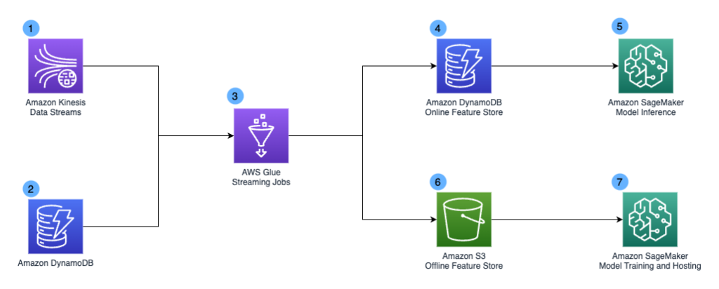
The following diagram illustrates the design of the Chime Streaming 2.0 system.

The design included the following key components:

  1. We have Amazon Kinesis Data Streams as our streaming data service to capture and store event streams at scale. Our stream pipelines capture various event types, including user enrollment events, user login events, card swipe events, peer-to-peer payments, and application screen actions.
  2. Amazon DynamoDB is another data source for our Streaming 2.0 system. It acts as the application backend and stores data such as blocked devices list and device-user mapping. We mainly use it as lookup tables in our pipeline.
  3. AWS Glue jobs form the backbone of our Streaming 2.0 system. The simple AWS Glue icon in the diagram represents thousands of AWS Glue jobs performing different transformations. To achieve the 5-15 seconds end-to-end data freshness service level agreement (SLA) for the Steaming 2.0 pipeline, we use streaming ETL jobs in AWS Glue to consume data from Kinesis Data Streams and apply near-real-time transformation. We choose AWS Glue mainly due to its serverless nature, which simplifies infrastructure management with automatic provisioning and worker management, and the ability to perform complex data transformations at scale.
  4. The AWS Glue streaming jobs generate derived fields and risk profiles that get stored in Amazon DynamoDB. We use Amazon DynamoDB as our online feature store due to its millisecond performance and scalability.
  5. Our applications call Amazon SageMaker Inference endpoints for fraud detections. The Amazon DynamoDB online feature store supports real-time inference with single digit millisecond query latency.
  6. We use Amazon Simple Storage Service (Amazon S3) as our offline feature store. It contains historical user activities and other derived ML features.
  7. Our data scientist team can access the dataset and perform ML model training and batch inferencing using Amazon SageMaker.

AWS Glue pipeline implementation deep dive

There are several key design principles for our AWS Glue Pipeline and the Streaming 2.0 project.

  • We want to democratize our data platform and make the data pipeline accessible to all Chime developers.
  • We want to implement cloud financial backend services and achieve cost efficiency.

To achieve data democratization, we needed to enable different personas in the organization to use the platform and define transformation jobs quickly, without worrying about the actual implementation details of the pipelines. The data infrastructure team built an abstraction layer on top of Spark and integrated services. This layer contained API wrappers over integrated services, job tags, scheduling configurations and debug tooling, hiding Spark and other lower-level complexities from end users. As a result, end users were able to define jobs with declarative YAML configurations and define transformation logic with SQL. This simplified the onboarding process and accelerated the implementation phase.

To achieve cost efficiency, our team built a cost attribution dashboard based on AWS cost allocation tags. We enforced tagging with the above abstraction layer and had clear cost attribution for all AWS Glue jobs down to the team level. This enabled us to track down less optimized jobs and work with job owners to implement best practices with impact-based priority. One common misconfiguration we found was sizing of AWS Glue jobs. With data democratization, many users lacked the knowledge to right-size their AWS Glue jobs. The AWS team introduced AWS Glue auto scaling to us as a solution. With AWS Glue Auto Scaling, we no longer needed to plan AWS Glue Spark cluster capacity in advance. We could just set the maximum number of workers and run the jobs. AWS Glue monitors the Spark application execution, and allocates more worker nodes to the cluster in near-real time after Spark requests more executors based on our workload requirements. We noticed a 30–45% cost saving across our AWS Glue Jobs once we turned on Auto Scaling.

Conclusion

In this post, we showed you how Chime’s Streaming 2.0 system allows us to ingest events and make them available to the decision platform just seconds after they are emitted from other services. This enables us to write better risk policies, provide fresher data for our machine learning models, and protect our members from unauthorized transactions on their accounts.

Over 500 developers in Chime are using this streaming pipeline and we ingest more than 1 million events per second. We follow the sizing and scaling process from the AWS Glue streaming ETL jobs best practices blog and land on a 1:1 mapping between Kinesis Shard and vCPU core. The end-to-end latency is less than 15 seconds, and it improves the model score calculation speed by 1200% compared to legacy implementation. This system has proven to be reliable, performant, and cost-effective at scale.

We hope this post will inspire your organization to build a real-time analytics platform using serverless technologies to accelerate your business goals.


About the Authors

Khandu Shinde Khandu Shinde is a Staff Engineer focused on Big Data Platforms and Solutions for Chime. He helps to make the platform scalable for Chime’s business needs with architectural direction and vision. He’s based in San Francisco where he plays cricket and watches movies.

Edward Paget Edward Paget is a Software Engineer working on building Chime’s capabilities to mitigate risk to ensure our members’ financial peace of mind. He enjoys being at the intersection of big data and programming language theory. He’s based in Chicago where he spends his time running along the lake shore.

Dylan Qu is a Specialist Solutions Architect focused on Big Data & Analytics with Amazon Web Services. He helps customers architect and build highly scalable, performant, and secure cloud-based solutions on AWS.

Optimize checkpointing in your Amazon Managed Service for Apache Flink applications with buffer debloating and unaligned checkpoints – Part 2

Post Syndicated from Lorenzo Nicora original https://aws.amazon.com/blogs/big-data/optimize-checkpointing-in-your-amazon-managed-service-for-apache-flink-applications-with-buffer-debloating-and-unaligned-checkpoints-part-2/

This post is a continuation of a two-part series. In the first part, we delved into Apache Flink‘s internal mechanisms for checkpointing, in-flight data buffering, and handling backpressure. We covered these concepts in order to understand how buffer debloating and unaligned checkpoints allow us to enhance performance for specific conditions in Apache Flink applications.

In Part 1, we introduced and examined how to use buffer debloating to improve in-flight data processing. In this post, we focus on unaligned checkpoints. This feature has been available since Apache Flink 1.11 and has received many improvements since then. Unaligned checkpoints help, under specific conditions, to reduce checkpointing time for applications suffering temporary backpressure, and can be now enabled in Amazon Managed Service for Apache Flink applications running Apache Flink 1.15.2 through a support ticket.

Even though this feature might improve performance for your checkpoints, if your application is constantly failing because of checkpoints timing out, or is suffering from having constant backpressure, you may require a deeper analysis and redesign of your application.

Aligned checkpoints

As discussed in Part 1, Apache Flink checkpointing allows applications to record state in case of failure. We’ve already discussed how checkpoints, when triggered by the job manager, signal all source operators to snapshot their state, which is then broadcasted as a special record called a checkpoint barrier. This process achieves exactly-once consistency for state in a distributed streaming application through the alignment of these barriers.

Let’s walk through the process of aligned checkpoints in a standard Apache Flink application. Remember that Apache Flink distributes the workload horizontally: each operator (a node in the logical flow of your application, including sources and sinks) is split into multiple sub-tasks based on its parallelism.

Barrier alignment

The alignment of checkpoint barriers is crucial for achieving exactly-once consistency in Apache Flink applications during checkpoint runs. To recap, when a job manager triggers a checkpoint, all sub-tasks of source operators receive a signal to initiate the checkpoint process. Each sub-task independently snapshots its state to the state backend and broadcasts a special record known as a checkpoint barrier to all outgoing streams.

When an application operates with a parallelism higher than 1, multiple instances of each task—referred to as sub-tasks—enable parallel message consumption and processing. A sub-task can receive distinct partitions of the same stream from different upstream sub-tasks, such as after a stream repartitioning with keyBy or rebalance operations. To maintain exactly-once consistency, all sub-tasks must wait for the arrival of all checkpoint barriers before taking a snapshot of the state. The following diagram illustrates the checkpoint barriers flow.

Checkpoint Barriers flow in the Buffer Queues

This phase is called checkpoint alignment. During alignment, the sub-task stops processing records from the partitions from which it has already received barriers, as shown in the following figure.

The first Barrier reaches the sub-task: Checkpointing Alignment begins

However, it continues to process partitions that are behind the barrier.

Processing continues only for partitions behind the barrier

When barriers from all upstream partitions have arrived, the sub-task takes a snapshot of its state.

Barrier alignment complete: snapshot state

Then it broadcasts the barrier downstream.

Emit Barriers downstream, and continue processing

The time a sub-task spends waiting for all barriers to arrive is measured by the checkpoint Alignment Duration metric, which can be observed in the Apache Flink UI.

If the application experiences backpressure, an increase in this metric could lead to longer checkpoint durations and even checkpoint failures due to timeouts. This is where unaligned checkpoints become a viable option to potentially enhance checkpointing performance.

Unaligned checkpoints

Unaligned checkpoints address situations where backpressure is not just a temporary spike, but results in timeouts for aligned checkpoints, due to barrier queuing within the stream. As discussed in Part 1, checkpoint barriers can’t overtake regular records. Therefore, significant backpressure can slow down the movement of barriers across the application, potentially causing checkpoint timeouts.

The objective of unaligned checkpoints is to enable barrier overtaking, allowing barriers to move swiftly from source to sink even when the data flow is slower than anticipated.

Building on what we saw in Part 1 concerning checkpoints and what aligned checkpoints are, let’s explore how unaligned checkpoints modify the checkpointing mechanism.

Upon emission, each source’s checkpoint barrier is injected into the stream flowing across sub-tasks. It travels from the source output network buffer queue into the input network buffer queue of the subsequent operator.

Upon the arrival of the first barrier in the input network buffer queue, the operator initially waits for barrier alignment. If the specified alignment timeout expires because not all barriers have reached the end of the input network buffer queue, the operator switches to unaligned checkpoint mode.

The alignment timeout can be set programmatically by env.getCheckpointConfig().setAlignedCheckpointTimeout(Duration.ofSeconds(30)), but modifying the default is not recommended in Apache Flink 1.15.

Checkpoint barriers flow in the buffer queues

The operator waits until all checkpoint barriers are present in the input network buffer queue before triggering the checkpoint. Unlike aligned checkpoints, the operator doesn’t need to wait for all barriers to reach the queue’s end, allowing the operator to have in-flight data from the buffer that hasn’t been processed before checkpoint initiation.

All barriers are in the input queues

After all barriers have arrived in the input network buffer queue, the operator advances the barrier to the end of the output network buffer queue. This enhances checkpointing speed because the barrier can smoothly traverse the application from source to sink, independent of the application’s end-to-end latency.

Barriers can overtake in-flight messages

After forwarding the barrier to the output network buffer queue, the operator initiates the snapshot of in-flight data between the barriers in the input and output network buffer queues, along with the snapshot of the state.

Although processing is momentarily paused during this process, the actual writing to the remote persistent state storage occurs asynchronously, preventing potential bottlenecks.

Snapshot state and in-flight messages

The local snapshot, encompassing in-flight messages and state, is saved asynchronously in the remote persistent state store, while the barrier continues its journey through the application.

Processing continues

When to use unaligned checkpoints

Remember, barrier alignment only occurs between partitions coming from different sub-tasks of the same operator. Therefore, if an operator is experiencing temporary backpressure, enabling unaligned checkpoints may be beneficial. This way, the application doesn’t have to wait for all barriers to reach the operator before performing the snapshot of state or moving the barrier forward.

Temporary backpressure could arise from the following:

  • A surge in data ingestion
  • Backfilling or catching up with historical data
  • Increased message processing time due to delayed external systems

Another scenario where unaligned checkpoints prove advantageous is when working with exactly-once sinks. Utilizing the two-phase commit sink function for exactly-once sinks, unaligned checkpoints can expedite checkpoint runs, thereby reducing end-to-end latency.

When not to use unaligned checkpoints

Unaligned checkpoints won’t reduce the time required for savepoints (called snapshots in the Amazon Managed Service for Apache Flink implementation) because savepoints exclusively utilize aligned checkpoints. Furthermore, because Apache Flink doesn’t permit concurrent unaligned checkpoints, savepoints won’t occur simultaneously with unaligned checkpoints, potentially elongating savepoint durations.

Unaligned checkpoints won’t fix any underlying issue in your application design. If your application is suffering from persistent backpressure or constant checkpointing timeouts, this might indicate data skewness or underprovisioning, which may require improving and tuning the application.

Using unaligned checkpoints with buffer debloating

One alternative for reducing the risks associated with an increased state size is to combine unaligned checkpoints with buffer debloating. This approach results in having less in-flight data to snapshot and store in the state, along with less data to be used for recovery in case of failure. This synergy facilitates enhanced performance and efficient checkpoint runs, leading to smaller checkpointing sizes and faster recovery times. When testing the use of unaligned checkpoints, we recommend doing so with buffer debloating to prevent the state size from increasing.

Limitations

Unaligned checkpoints are subject to the following limitations:

  • They provide no benefit for operators with a parallelism of 1.
  • They only improve performance for operators where barrier alignment would have occurred. This alignment happens only if records are coming from different sub-tasks of the same operator, for example, through repartitioning or keyBy operations.
  • Operators receiving input from multiple sources or participating in joins might not experience improvements, because the operator would be receiving data from different operators in those cases.
  • Although checkpoint barriers can surpass records in the network’s buffer queue, this won’t occur if the sub-task is currently processing a message. If processing a message takes too much time (for example, a flat-map operation emitting numerous records for each input record), barrier handling will be delayed.
  • As we have seen, savepoints always use aligned checkpoints. If the savepoints of your applications are slow due to barrier alignment, unaligned checkpoints will not help.
  • Additional limitations affect watermarks, message ordering, and broadcast state in recovery. For more details, refer to Limitations.

Considerations

Considerations for implementing unaligned checkpoints:

  • Unaligned checkpoints introduce additional I/O to checkpoint storage
  • Checkpoints encompass not only operator state but also in-flight data within network buffer queues, leading to increased state size

Recommendations

We offer the following recommendations:

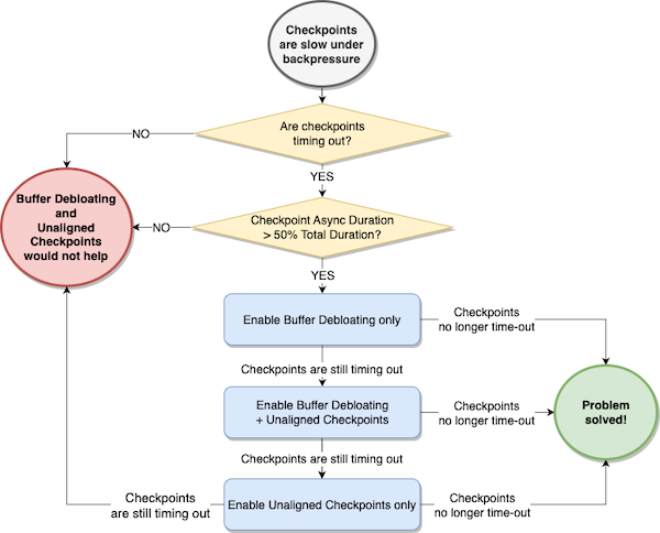
  • Consider enabling unaligned checkpoints only if both of the following conditions are true:
  • Checkpoints are timing out.
  • The average checkpoint Async Duration of any operator is more than 50% of the total checkpoint duration for the operator (sum of Sync Duration + Async Duration).
  • Consider enabling buffer debloating first, and evaluate whether it solves the problem of checkpoints timing out.
  • If buffer debloating doesn’t help, consider enabling unaligned checkpoints along with buffer debloating. Buffer debloating mitigates the drawbacks of unaligned checkpoints, reducing the amount of in-flight data.
  • If unaligned checkpoints and buffer debloating together don’t improve checkpoint alignment duration, consider testing unaligned checkpoints alone.

Decision flow

Finally, but most importantly, always test unaligned checkpoints in a non-production environment first, running some comparative performance testing with a realistic workload, and verify that unaligned checkpoints actually reduce checkpoint duration.

Conclusion

This two-part series explored advanced strategies for optimizing checkpointing within your Amazon Managed Service for Apache Flink applications. By harnessing the potential of buffer debloating and unaligned checkpoints, you can unlock significant performance improvements and streamline checkpoint processes. However, it’s important to understand when these techniques will provide improvements and when they will not. If you believe your application may benefit from checkpoint performance improvement, you can enable these features in your Amazon Managed Service For Apache Flink version 1.15 applications. We recommend first enabling buffer debloating and testing the application. If you are still not seeing the expected outcome, enable buffer debloating with unaligned checkpoints. This way, you can immediately reduce the state size and the additional I/O to state backends. Lastly, you may try using unaligned checkpoints by itself, bearing in mind the considerations we’ve mentioned.

With a deeper understanding of these techniques and their applicability, you are better equipped to maximize the efficiency of checkpoints and mitigate the effect of backpressure in your Apache Flink application.


About the Authors

Lorenzo NicoraLorenzo Nicora works as Senior Streaming Solution Architect helping customers across EMEA. He has been building cloud-native, data-intensive systems for over 25 years, working in the finance industry both through consultancies and for FinTech product companies. He has leveraged open-source technologies extensively and contributed to several projects, including Apache Flink.

Francisco MorilloFrancisco Morillo is a Streaming Solutions Architect at AWS. Francisco works with AWS customers helping them design real-time analytics architectures using AWS services, supporting Amazon Managed Streaming for Apache Kafka (Amazon MSK) and AWS’s managed offering for Apache Flink.
Optimize checkpointing in your Amazon Managed Service for Apache Flink applications with buffer debloating and unaligned checkpoints – Part 1

Post Syndicated from Lorenzo Nicora original https://aws.amazon.com/blogs/big-data/part-1-optimize-checkpointing-in-your-amazon-managed-service-for-apache-flink-applications-with-buffer-debloating-and-unaligned-checkpoints/

This post is the first of a two-part series regarding checkpointing mechanisms and in-flight data buffering. In this first part, we explain some of the fundamental Apache Flink internals and cover the buffer debloating feature. In the second part, we focus on unaligned checkpoints.

Apache Flink is an open-source distributed engine for stateful processing over unbounded datasets (streams) and bounded datasets (batches). Amazon Managed Service for Apache Flink, formerly known as Amazon Kinesis Data Analytics, is the AWS service offering fully managed Apache Flink.

Apache Flink is designed for stateful processing at scale, for high throughput and low latency. It scales horizontally, distributing processing and state across multiple nodes, and is designed to withstand failures without compromising the exactly-once consistency it provides.

Internally, Apache Flink uses clever mechanisms to maintain exactly-once state consistency, while also optimizing for throughput and reduced latency. The default behavior works well for most use cases. Recent versions introduced two functionalities that can be optionally enabled to improve application performance under particular conditions: buffer debloating and unaligned checkpoints.

Buffer debloating and unaligned checkpoints can be enabled on Amazon Managed Service for Apache Flink version 1.15.

To understand how these functionalities can help and when to use them, we need to dive deep into some of the fundamental internal mechanisms of Apache Flink: checkpointing, in-flight data buffering, and backpressure.

Maintaining state consistency through failures with checkpointing

Apache Flink checkpointing periodically saves the internal application state for recovering in case of failure. Each of the distributed components of an application asynchronously snapshots its state to an external persistent datastore. The challenge is taking snapshots guaranteeing exactly-once consistency. A naïve “stop-the-world, take a snapshot” implementation would never meet the high throughput and low latency goals Apache Flink has been designed for.

Let’s walk through the process of checkpointing in a simple streaming application.

As shown in the following figure, Apache Flink distributes the work horizontally. Each operator (a node in the logical flow of your application, including sources and sinks) is split into multiple sub-tasks, based on its parallelism. The application is coordinated by a job manager. Checkpoints are periodically initiated by the job manager, sending a signal to all source operators’ sub-tasks.

Checkpoint initiated by the Job Manager

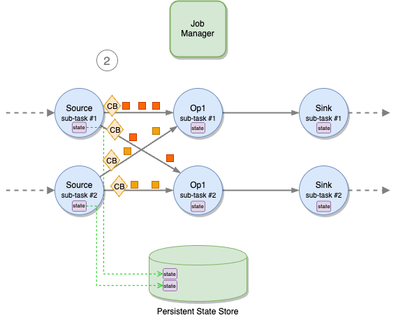
On receiving the signal, each source sub-task independently snapshots its state (for example, the offsets of the Kafka topic it is consuming) to a persistent storage, and then broadcasts a special record called checkpoint barrier (“CB” in the following diagrams) to all outgoing streams. Checkpoint barriers work similarly to watermarks in Apache Flink, flowing in-bands, along with normal records. A barrier does not overtake normal records and is not overtaken.

Source operators emit checkpoint bariers

When a downstream operator’s sub-task receives all checkpoint barriers from all input channels, it starts snapshotting its state.

A sub-task does not pause processing while saving its state to the remote, persistent state backend. This is a two-phase operation. First, the sub-task takes a snapshot of the state, on the local file system or in memory, depending on application configuration. This operation is blocking but very fast. When the snapshot is complete, it restarts processing records, while the state is asynchronously saved to the external, persistent state store. When the state is successfully saved to the state store, the sub-task acknowledges to the job manager that its checkpointing is complete.

The time a sub-task spends on the synchronous and asynchronous parts of the checkpoint is measured by Sync Duration and Async Duration metrics, shown by the Apache Flink UI. It is then asynchronously sent to the backend. After the fast snapshot, the sub-task restarts processing messages. The backend notifies the sub-task when the state has been successfully saved. The sub-task, in turn, sends an acknowledgment to the job manager that checkpointing is complete.

Sub-tasks acknowledge checkpoint completion

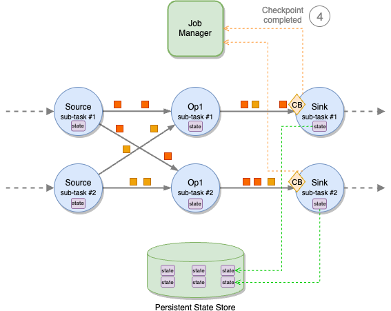
Checkpoint barriers propagate through all operators, down to the sinks. When all sink sub-tasks have acknowledged the checkpoint to the job manager, the checkpoint is declared complete and can be used to recover the application, for example in case of failure.

Sink operators acknowledge checkpoint is complete

Checkpoint barrier alignment

A sub-task may receive different partitions of the same stream from different upstream sub-tasks, for example when a stream is repartitioned with a keyBy or a rebalance. Each upstream sub-task will emit a checkpoint barrier independently. To maintain exactly-once consistency, the sub-task must wait for the barriers to arrive on all input partitions before taking a snapshot of its state.

This phase is called checkpoint alignment. During the alignment, the sub-task stops processing records from the partitions it already received the barrier from and continues processing the partitions that are behind the barrier.

After the barriers from all upstream partitions have arrived, the sub-task takes the snapshot of its state and then broadcasts the barrier downstream.

The time spent by a sub-task while aligning barriers is measured by the Checkpoint Alignment Duration metric, shown by the Apache Flink UI.

Checkpoint barrier alignment

In-flight data buffering

To optimize for throughput, Apache Flink tries to keep each sub-task always busy. This is achieved by transmitting records over the network in blocks and by buffering in-flight data. Note that this is data transmission optimization; Flink operators always process records one at the time.

Data is handed over between sub-tasks in units called network buffers. A network buffer has a fixed size, in bytes.

Sub-tasks also buffer in-flight input and output data. These buffers are called network buffer queues. Each queue is composed of multiple network buffers. Each sub-task has an input network buffer queue for each upstream sub-task and an output network buffer queue for each downstream sub-task.

Each record emitted by the sub-task is serialized, put into network buffers, and published to the output network buffer queue. To use all the available space, multiple messages can be packed into a single network buffer or split across subsequent network buffers.

A separate thread sends full network buffers over the network, where they are stored in the destination sub-task’s input network buffer queue.

When the destination sub-task thread is free, it deserializes the network buffers, rebuilds the records, and processes them one at a time.

Network Buffer Queue

Backpressure

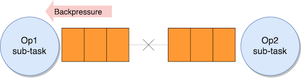
If a sub-task can’t keep up with processing records at the same pace they are received, the input queue fills up. When the input queue is full, the upstream sub-task stops sending data.

Data accumulates in the sender’s output queue. When this is also full, the sender sub-task stops processing records, accumulating received data in its own input queue, and the effects propagates upstream.

This is the backpressure that Apache Flink uses to control the internal flow, preventing slow operators from being overwhelmed by slowing down the upstream flow. Backpressure is a safety mechanism to maximize the application throughput. It can be temporary, in case of an unexpected peak of ingested data, for example. If not temporary, it is usually the symptom—not the cause—that the application is not designed correctly or it has insufficient resources to process the workload.

Full Network Buffer Queue generates backpressure

In-flight buffering and checkpoint barriers

As checkpoint barriers flow with normal records, they also flow in the network buffers, through the input and output queues. In normal conditions, barriers don’t overtake records, and they are never overtaken. If records are queueing up due to backpressure, checkpoint barriers are also stuck in the queue, taking longer time to propagate from the sources to the sinks, delaying the completion of the checkpoint.

In the second part of this series, we will see how unaligned checkpoints can let barriers overtake records under specific conditions. For now, let’s see how we can optimize the size of input and output queues with buffer debloating.

Buffer debloating to optimize in-flight data

The default network buffer queue size is a good compromise for most applications. You can modify this size, but it applies to all sub-tasks, and it may be difficult to optimize this one-size-fits-all across different operators.

Longer queues support bigger throughout, but they may slow down checkpoint barriers that have to go through longer queues, causing longer End to End Checkpoint Duration. Ideally, the amount of in-flight data should be adjusted based on the actual throughput.

In version 1.14, Apache Flink introduced buffer debloating, which can be enabled to adjust in-flight data of each sub-task, based on the current throughput the sub-task is processing, and periodically reassess and readjust it.

How buffer debloating helps your application

Consider a streaming application, ingesting records from a streaming source and publishing the results to a streaming destination after some transformations. Under normal conditions, the application is sized to process the incoming throughput smoothly. Our destination has limited capacity, for example a Kafka topic throttled via quotas, sufficient to handle the normal throughput, with some margin.

In-flight data buffering under normal throughput

Imagine that the ingestion throughput has occasional peaks. These peaks exceed the limits of the streaming destination (throughput quota of the Kafka topic), which starts throttling.

Full in-flight data buffer to the sink backpressure the preceding operator

Because the sink can’t process the full throughput, in-flight data accumulates upstream of the sink, causing backpressure on the upstream operator. The effect eventually propagates up to the source, and the source starts lagging behind the most recent record in the source stream.

Backpressure propagates upstream, up to the source operator

As long this is a temporary condition, backpressure and lagging are not a problem per se, as long as the application is able to catch up when the peak has finished.

Unfortunately, accumulating in-flight data also slows down the propagation of the checkpoint barriers. Checkpoint End to End Duration goes up, and checkpoints may eventually time out.

Full in-flight data buffers slow down checkpoint barrier propagation, under backpressure

The situation is even worse if the sink uses two-phase commit for exactly-once guarantees. For example, KafkaSink uses Kafka transactions committed on checkpoints. If checkpoints become too slow, transactions are committed later, significantly increasing the latency of any downstream consumer using a read-committed isolation level.

Slow checkpoints under backpressure may also cause a vicious cycle. A slowed-down application eventually crashes, and recovers from the last checkpoint that is quite old. This causes a long reprocessing that, in turn, induces more backpressure and even slower checkpoints.

In this case, buffer debloating can help by adjusting the amount of in-flight data based on the throughput each sub-task is actually processing. When a sub-task is throttled by backpressure, the amount of in-flight data is reduced, also reducing the time checkpoint barriers take to go through all operators. Checkpoint End to End Duration goes down, and checkpoints do not time out.

Buffer debloating internals

Buffer debloating estimates the throughput a sub-task is capable of processing, assuming no idling, and limits the upstream in-flight data buffers to contain just enough data to be processed in 1 second (by default).

For efficiency, network buffers in the queues are fixed. Buffer debloating caps the usable size of each network buffer, making it smaller when the sub-task is processing slowly.

Buffer debloating speed up barrier propagation, reducing the volume of in-flight data

The benefits of less in-flight data depends on whether Apache Flink is using standard checkpoint alignment, the default behavior described so far, or unaligned checkpoints. We will examine unaligned checkpoints in the second part of this series, but let’s see the effect of buffer debloating, briefly.

  • With aligned checkpoints (default behavior) – Less in-flight data makes checkpoint barrier propagation faster, ultimately reducing the end-to-end checkpoint duration but also making it more predictable
  • With unaligned checkpoints (optional) – Less in-flight data reduces the amount of in-flight records stored with the checkpoint, ultimately reducing the checkpoint size

What buffer debloating does not do

Note that the problem we are trying to solve is slow checkpointing (or excessive checkpointing size, with unaligned checkpoints). Buffer debloating helps making checkpointing faster.

Buffer debloating does not remove backpressure. Backpressure is the internal protective mechanism that Apache Flink uses when some part of the application is not able to cope with the incoming throughput. To reduce backpressure, you have to work on other aspects of the application. When backpressure is only temporary, for example under peak conditions, the only way of removing it would be sizing the end-to-end system for the peak, rather than normal workload. But this could be impossible or too expensive.

Buffer debloating helps reduce and keep checkpoint duration stable under exceptional and temporary conditions. If an application experiences backpressure under its normal workload, or checkpoints are too slow under normal conditions, you should investigate the implementation of your application to understand the root cause.

When the automatic throughput prediction fails

Buffer debloating doesn’t have any particular drawback, but in corner cases, the mechanism may incorrectly estimate the throughput, and the resulting amount of in-flight data may not be optimal.

Estimating the throughput is complex when an operator receives data from multiple upstream operators, connected streams or unions, with very different throughput. It may also take time to adjust to a sudden spike, causing a temporary suboptimal buffering.

  • Too small in-flight data may reduce the throughput the sub-task can process (it will be idling), causing more backpressure upstream
  • Too large buffers may slow down checkpointing and increase the checkpoint size (with unaligned checkpoints)

Conclusion

The checkpointing mechanism makes Apache Flink fault tolerant, providing exactly-once state consistency. In-flight data buffering and backpressure control the data flow within the distributed streaming application maximize the throughput. Apache Flink default behaviors and configurations are good for most workloads.

The effectiveness of buffer debloating depends on the characteristics of the workload and the application. The general recommendation is to test the functionality in a non-production environment with a realistic workload to verify it actually helps with your use case.

You can request to enable buffer debloating on your Amazon Managed Service for Apache Flink application.

Under particular conditions, the combined effect of backpressure and in-flight data buffering may slow down checkpointing, increase checkpointing size (with unaligned checkpoints), and even cause checkpoints to fail. In these cases, enabling unaligned checkpointing may help reduce checkpoint duration or size.

In the second part of this series, we will understand better unaligned checkpoints and how they can help your application checkpointing efficiently in presence of backpressure, especially in combination with buffer debloating.


About the Authors

Lorenzo NicoraLorenzo Nicora works as Senior Streaming Solution Architect at AWS, helping customers across EMEA. He has been building cloud-native, data-intensive systems for over 25 years, working in the finance industry both through consultancies and for FinTech product companies. He has leveraged open-source technologies extensively and contributed to several projects, including Apache Flink.

Francisco MorilloFrancisco Morillo is a Streaming Solutions Architect at AWS. Francisco works with AWS customers helping them design real-time analytics architectures using AWS services, supporting Amazon Managed Streaming for Apache Kafka (Amazon MSK) and AWS’s managed offering for Apache Flink.
Simplify operational data processing in data lakes using AWS Glue and Apache Hudi

Post Syndicated from Ravi Itha original https://aws.amazon.com/blogs/big-data/simplify-operational-data-processing-in-data-lakes-using-aws-glue-and-apache-hudi/

The Analytics specialty practice of AWS Professional Services (AWS ProServe) helps customers across the globe with modern data architecture implementations on the AWS Cloud. A modern data architecture is an evolutionary architecture pattern designed to integrate a data lake, data warehouse, and purpose-built stores with a unified governance model. It focuses on defining standards and patterns to integrate data producers and consumers and move data between data lakes and purpose-built data stores securely and efficiently. Out of the many data producer systems that feed data to a data lake, operational databases are most prevalent, where operational data is stored, transformed, analyzed, and finally used to enhance business operations of an organization. With the emergence of open storage formats such as Apache Hudi and its native support from AWS Glue for Apache Spark, many AWS customers have started adding transactional and incremental data processing capabilities to their data lakes.

AWS has invested in native service integration with Apache Hudi and published technical contents to enable you to use Apache Hudi with AWS Glue (for example, refer to Introducing native support for Apache Hudi, Delta Lake, and Apache Iceberg on AWS Glue for Apache Spark, Part 1: Getting Started). In AWS ProServe-led customer engagements, the use cases we work on usually come with technical complexity and scalability requirements. In this post, we discuss a common use case in relation to operational data processing and the solution we built using Apache Hudi and AWS Glue.

Use case overview

AnyCompany Travel and Hospitality wanted to build a data processing framework to seamlessly ingest and process data coming from operational databases (used by reservation and booking systems) in a data lake before applying machine learning (ML) techniques to provide a personalized experience to its users. Due to the sheer volume of direct and indirect sales channels the company has, its booking and promotions data are organized in hundreds of operational databases with thousands of tables. Of those tables, some are larger (such as in terms of record volume) than others, and some are updated more frequently than others. In the data lake, the data to be organized in the following storage zones:

  1. Source-aligned datasets – These have an identical structure to their counterparts at the source
  2. Aggregated datasets – These datasets are created based on one or more source-aligned datasets
  3. Consumer-aligned datasets – These are derived from a combination of source-aligned, aggregated, and reference datasets enriched with relevant business and transformation logics, usually fed as inputs to ML pipelines or any consumer applications

The following are the data ingestion and processing requirements:

  1. Replicate data from operational databases to the data lake, including insert, update, and delete operations.
  2. Keep the source-aligned datasets up to date (typically within the range of 10 minutes to a day) in relation to their counterparts in the operational databases, ensuring analytics pipelines refresh consumer-aligned datasets for downstream ML pipelines in a timely fashion. Moreover, the framework should consume compute resources as optimally as possible per the size of the operational tables.
  3. To minimize DevOps and operational overhead, the company wanted to templatize the source code wherever possible. For example, to create source-aligned datasets in the data lake for 3,000 operational tables, the company didn’t want to deploy 3,000 separate data processing jobs. The smaller the number of jobs and scripts, the better.
  4. The company wanted the ability to continue processing operational data in the secondary Region in the rare event of primary Region failure.

As you can guess, the Apache Hudi framework can solve the first requirement. Therefore, we will put our emphasis on the other requirements. We begin with a Data lake reference architecture followed by an overview of operational data processing framework. By showing you our open-source solution on GitHub, we delve into framework components and walk through their design and implementation aspects. Finally, by testing the framework, we summarize how it meets the aforementioned requirements.

Data lake reference architecture

Let’s begin with a big picture: a data lake solves a variety of analytics and ML use cases dealing with internal and external data producers and consumers. The following diagram represents a generic data lake architecture. To ingest data from operational databases to an Amazon Simple Storage Service (Amazon S3) staging bucket of the data lake, either AWS Database Migration Service (AWS DMS) or any AWS partner solution from AWS Marketplace that has support for change data capture (CDC) can fulfill the requirement. AWS Glue is used to create source-aligned and consumer-aligned datasets and separate AWS Glue jobs to do feature engineering part of ML engineering and operations. Amazon Athena is used for interactive querying and AWS Lake Formation is used for access controls.

Data Lake Reference Architecture

Operational data processing framework

The operational data processing (ODP) framework contains three components: File Manager, File Processor, and Configuration Manager. Each component runs independently to solve a portion of the operational data processing use case. We have open-sourced this framework on GitHub—you can clone the code repo and inspect it while we walk you through the design and implementation of the framework components. The source code is organized in three folders, one for each component, and if you customize and adopt this framework for your use case, we recommend promoting these folders as separate code repositories in your version control system. Consider using the following repository names:

  1. aws-glue-hudi-odp-framework-file-manager
  2. aws-glue-hudi-odp-framework-file-processor
  3. aws-glue-hudi-odp-framework-config-manager

With this modular approach, you can independently deploy the components to your data lake environment by following your preferred CI/CD processes. As illustrated in the preceding diagram, these components are deployed in conjunction with a CDC solution.

Component 1: File Manager

File Manager detects files emitted by a CDC process such as AWS DMS and tracks them in an Amazon DynamoDB table. As shown in the following diagram, it consists of an Amazon EventBridge event rule, an Amazon Simple Queue Service (Amazon SQS) queue, an AWS Lambda function, and a DynamoDB table. The EventBridge rule uses Amazon S3 Event Notifications to detect the arrival of CDC files in the S3 bucket. The event rule forwards the object event notifications to the SQS queue as messages. The File Manager Lambda function consumes those messages, parses the metadata, and inserts the metadata to the DynamoDB table odpf_file_tracker. These records will then be processed by File Processor, which we discuss in the next section.

ODPF Component: File Manager

Component 2: File Processor

File Processor is the workhorse of the ODP framework. It processes files from the S3 staging bucket, creates source-aligned datasets in the raw S3 bucket, and adds or updates metadata for the datasets (AWS Glue tables) in the AWS Glue Data Catalog.

We use the following terminology when discussing File Processor:

  1. Refresh cadence – This represents the data ingestion frequency (for example, 10 minutes). It usually goes with AWS Glue worker type (one of G.1X, G.2X, G.4X, G.8X, G.025X, and so on) and batch size.
  2. Table configuration – This includes the Hudi configuration (primary key, partition key, pre-combined key, and table type (Copy on Write or Merge on Read)), table data storage mode (historical or current snapshot), S3 bucket used to store source-aligned datasets, AWS Glue database name, AWS Glue table name, and refresh cadence.
  3. Batch size – This numeric value is used to split tables into smaller batches and process their respective CDC files in parallel. For example, a configuration of 50 tables with a 10-minute refresh cadence and a batch size of 5 results in a total of 10 AWS Glue job runs, each processing CDC files for 5 tables.
  4. Table data storage mode – There are two options:
    • Historical – This table in the data lake stores historical updates to records (always append).
    • Current snapshot – This table in the data lake stores latest versioned records (upserts) with the ability to use Hudi time travel for historical updates.
  5. File processing state machine – It processes CDC files that belong to tables that share a common refresh cadence.
  6. EventBridge rule association with the file processing state machine – We use a dedicated EventBridge rule for each refresh cadence with the file processing state machine as target.
  7. File processing AWS Glue job – This is a configuration-driven AWS Glue extract, transform, and load (ETL) job that processes CDC files for one or more tables.

File Processor is implemented as a state machine using AWS Step Functions. Let’s use an example to understand this. The following diagram illustrates running File Processor state machine with a configuration that includes 18 operational tables, a refresh cadence of 10 minutes, a batch size of 5, and an AWS Glue worker type of G.1X.

ODP framework component: File Processor

The workflow includes the following steps:

  1. The EventBridge rule triggers the File Processor state machine every 10 minutes.
  2. Being the first state in the state machine, the Batch Manager Lambda function reads configurations from DynamoDB tables.
  3. The Lambda function creates four batches: three of them will be mapped to five operational tables each, and the fourth one is mapped to three operational tables. Then it feeds the batches to the Step Functions Map state.
  4. For each item in the Map state, the File Processor Trigger Lambda function will be invoked, which in turn runs the File Processor AWS Glue job.
  5. Each AWS Glue job performs the following actions:
    • Checks the status of an operational table and acquires a lock when it is not processed by any other job. The odpf_file_processing_tracker DynamoDB table is used for this purpose. When a lock is acquired, it inserts a record in the DynamoDB table with the status updating_table for the first time; otherwise, it updates the record.
    • Processes the CDC files for the given operational table from the S3 staging bucket and creates a source-aligned dataset in the S3 raw bucket. It also updates technical metadata in the AWS Glue Data Catalog.
    • Updates the status of the operational table to completed in the odpf_file_processing_tracker table. In case of processing errors, it updates the status to refresh_error and logs the stack trace.
    • It also inserts this record into the odpf_file_processing_tracker_history DynamoDB table along with additional details such as insert, update, and delete row counts.
    • Moves the records that belong to successfully processed CDC files from odpf_file_tracker to the odpf_file_tracker_history table with file_ingestion_status set to raw_file_processed.
    • Moves to the next operational table in the given batch.
    • Note: a failure to process CDC files for one of the operational tables of a given batch does not impact the processing of other operational tables.

Component 3: Configuration Manager

Configuration Manager is used to insert configuration details to the odpf_batch_config and odpf_raw_table_config tables. To keep this post concise, we provide two architecture patterns in the code repo and leave the implementation details to you.

Solution overview

Let’s test the ODP framework by replicating data from 18 operational tables to a data lake and creating source-aligned datasets with 10-minute refresh cadence. We use Amazon Relational Database Service (Amazon RDS) for MySQL to set up an operational database with 18 tables, upload the New York City Taxi – Yellow Trip Data dataset, set up AWS DMS to replicate data to Amazon S3, process the files using the framework, and finally validate the data using Amazon Athena.

Create S3 buckets

For instructions on creating an S3 bucket, refer to Creating a bucket. For this post, we create the following buckets:

  1. odpf-demo-staging-EXAMPLE-BUCKET – You will use this to migrate operational data using AWS DMS
  2. odpf-demo-raw-EXAMPLE-BUCKET – You will use this to store source-aligned datasets
  3. odpf-demo-code-artifacts-EXAMPLE-BUCKET – You will use this to store code artifacts

Deploy File Manager and File Processor

Deploy File Manager and File Processor by following instructions from this README and this README, respectively.

Set up Amazon RDS for MySQL

Complete the following steps to set up Amazon RDS for MySQL as the operational data source:

  1. Provision Amazon RDS for MySQL. For instructions, refer to Create and Connect to a MySQL Database with Amazon RDS.
  2. Connect to the database instance using MySQL Workbench or DBeaver.
  3. Create a database (schema) by running the SQL command CREATE DATABASE taxi_trips;.
  4. Create 18 tables by running the SQL commands in the ops_table_sample_ddl.sql script.

Populate data to the operational data source

Complete the following steps to populate data to the operational data source:

  1. To download the New York City Taxi – Yellow Trip Data dataset for January 2021 (Parquet file), navigate to NYC TLC Trip Record Data, expand 2021, and choose Yellow Taxi Trip records. A file called yellow_tripdata_2021-01.parquet will be downloaded to your computer.
  2. On the Amazon S3 console, open the bucket odpf-demo-staging-EXAMPLE-BUCKET and create a folder called nyc_yellow_trip_data.
  3. Upload the yellow_tripdata_2021-01.parquet file to the folder.
  4. Navigate to the bucket odpf-demo-code-artifacts-EXAMPLE-BUCKET and create a folder called glue_scripts.
  5. Download the file load_nyc_taxi_data_to_rds_mysql.py from the GitHub repo and upload it to the folder.
  6. Create an AWS Identity and Access Management (IAM) policy called load_nyc_taxi_data_to_rds_mysql_s3_policy. For instructions, refer to Creating policies using the JSON editor. Use the odpf_setup_test_data_glue_job_s3_policy.json policy definition.
  7. Create an IAM role called load_nyc_taxi_data_to_rds_mysql_glue_role. Attach the policy created in the previous step.
  8. On the AWS Glue console, create a connection for Amazon RDS for MySQL. For instructions, refer to Adding a JDBC connection using your own JDBC drivers and Setting up a VPC to connect to Amazon RDS data stores over JDBC for AWS Glue. Name the connection as odpf_demo_rds_connection.
  9. In the navigation pane of the AWS Glue console, choose Glue ETL jobs, Python Shell script editor, and Upload and edit an existing script under Options.
  10. Choose the file load_nyc_taxi_data_to_rds_mysql.py and choose Create.
  11. Complete the following steps to create your job:
    • Provide a name for the job, such as load_nyc_taxi_data_to_rds_mysql.
    • For IAM role, choose load_nyc_taxi_data_to_rds_mysql_glue_role.
    • Set Data processing units to 1/16 DPU.
    • Under Advanced properties, Connections, select the connection you created earlier.
    • Under Job parameters, add the following parameters:
      • input_sample_data_path = s3://odpf-demo-staging-EXAMPLE-BUCKET/nyc_yellow_trip_data/yellow_tripdata_2021-01.parquet
      • schema_name = taxi_trips
      • table_name = table_1
      • rds_connection_name = odpf_demo_rds_connection
    • Choose Save.
  12. On the Actions menu, run the job.
  13. Go back to your MySQL Workbench or DBeaver and validate the record count by running the SQL command select count(1) row_count from taxi_trips.table_1. You will get an output of 1369769.
  14. Populate the remaining 17 tables by running the SQL commands from the populate_17_ops_tables_rds_mysql.sql script.
  15. Get the row count from the 18 tables by running the SQL commands from the ops_data_validation_query_rds_mysql.sql script. The following screenshot shows the output.
    Record volumes (for 18 Tables) in Operational Database

Configure DynamoDB tables

Complete the following steps to configure the DynamoDB tables:

  1. Download file load_ops_table_configs_to_ddb.py from the GitHub repo and upload it to the folder glue_scripts in the S3 bucket odpf-demo-code-artifacts-EXAMPLE-BUCKET.
  2. Create an IAM policy called load_ops_table_configs_to_ddb_ddb_policy. Use the odpf_setup_test_data_glue_job_ddb_policy.json policy definition.
  3. Create an IAM role called load_ops_table_configs_to_ddb_glue_role. Attach the policy created in the previous step.
  4. On the AWS Glue console, choose Glue ETL jobs, Python Shell script editor, and Upload and edit an existing script under Options.
  5. Choose the file load_ops_table_configs_to_ddb.py and choose Create.
  6. Complete the following steps to create a job:
    • Provide a name, such as load_ops_table_configs_to_ddb.
    • For IAM role, choose load_ops_table_configs_to_ddb_glue_role.
    • Set Data processing units to 1/16 DPU.
    • Under Job parameters, add the following parameters
      • batch_config_ddb_table_name = odpf_batch_config
      • raw_table_config_ddb_table_name = odpf_demo_taxi_trips_raw
      • aws_region = e.g., us-west-1
    • Choose Save.
  7. On the Actions menu, run the job.
  8. On the DynamoDB console, get the item count from the tables. You will find 1 item in the odpf_batch_config table and 18 items in the odpf_demo_taxi_trips_raw table.

Set up a database in AWS Glue

Complete the following steps to create a database:

  1. On the AWS Glue console, under Data catalog in the navigation pane, choose Databases.
  2. Create a database called odpf_demo_taxi_trips_raw.

Set up AWS DMS for CDC

Complete the following steps to set up AWS DMS for CDC:

  1. Create an AWS DMS replication instance. For Instance class, choose dms.t3.medium.
  2. Create a source endpoint for Amazon RDS for MySQL.
  3. Create target endpoint for Amazon S3. To configure the S3 endpoint settings, use the JSON definition from dms_s3_endpoint_setting.json.
  4. Create an AWS DMS task.
    • Use the source and target endpoints created in the previous steps.
    • To create AWS DMS task mapping rules, use the JSON definition from dms_task_mapping_rules.json.
    • Under Migration task startup configuration, select Automatically on create.
  5. When the AWS DMS task starts running, you will see a task summary similar to the following screenshot.
    DMS Task Summary
  6. In the Table statistics section, you will see an output similar to the following screenshot. Here, the Full load rows and Total rows columns are important metrics whose counts should match with the record volumes of the 18 tables in the operational data source.
    DMS Task Statistics
  7. As a result of successful full load completion, you will find Parquet files in the S3 staging bucket—one Parquet file per table in a dedicated folder, similar to the following screenshot. Similarly, you will find 17 such folders in the bucket.
    DMS Output in S3 Staging Bucket for Table 1

File Manager output

The File Manager Lambda function consumes messages from the SQS queue, extracts metadata for the CDC files, and inserts one item per file to the odpf_file_tracker DynamoDB table. When you check the items, you will find 18 items with file_ingestion_status set to raw_file_landed, as shown in the following screenshot.

CDC Files in File Tracker DynamoDB Table

File Processor output

  1. On the subsequent tenth minute (since the activation of the EventBridge rule), the event rule triggers the File Processor state machine. On the Step Functions console, you will notice that the state machine is invoked, as shown in the following screenshot.
    File Processor State Machine Run Summary
  2. As shown in the following screenshot, the Batch Generator Lambda function creates four batches and constructs a Map state for parallel running of the File Processor Trigger Lambda function.
    File Processor State Machine Run Details
  3. Then, the File Processor Trigger Lambda function runs the File Processor Glue Job, as shown in the following screenshot.
    File Processor Glue Job Parallel Runs
  4. Then, you will notice that the File Processor Glue Job runs create source-aligned datasets in Hudi format in the S3 raw bucket. For Table 1, you will see an output similar to the following screenshot. There will be 17 such folders in the S3 raw bucket.
    Data in S3 raw bucket
  5. Finally, in AWS Glue Data Catalog, you will notice 18 tables created in the odpf_demo_taxi_trips_raw database, similar to the following screenshot.
    Tables in Glue Database

Data validation

Complete the following steps to validate the data:

  1. On the Amazon Athena console, open the query editor, and select a workgroup or create a new workgroup.
  2. Choose AwsDataCatalog for Data source and odpf_demo_taxi_trips_raw for Database.
  3. Run the raw_data_validation_query_athena.sql SQL query. You will get an output similar to the following screenshot.
    Raw Data Validation via Amazon Athena

Validation summary: The counts in Amazon Athena match with the counts of the operational tables and it proves that the ODP framework has processed all the files and records successfully. This concludes the demo. To test additional scenarios, refer to Extended Testing in the code repo.

Outcomes

Let’s review how the ODP framework addressed the aforementioned requirements.

  1. As discussed earlier in this post, by logically grouping tables by refresh cadence and associating them to EventBridge rules, we ensured that the source-aligned tables are refreshed by the File Processor AWS Glue jobs. With the AWS Glue worker type configuration setting, we selected the appropriate compute resources while running the AWS Glue jobs (the instances of the AWS Glue job).
  2. By applying table-specific configurations (from odpf_batch_config and odpf_raw_table_config) dynamically, we were able to use one AWS Glue job to process CDC files for 18 tables.
  3. You can use this framework to support a variety of data migration use cases that require quicker data migration from on-premises storage systems to data lakes or analytics platforms on AWS. You can reuse File Manager as is and customize File Processor to work with other storage frameworks such as Apache Iceberg, Delta Lake, and purpose-built data stores such as Amazon Aurora and Amazon Redshift.
  4. To understand how the ODP framework met the company’s disaster recovery (DR) design criterion, we first need to understand the DR architecture strategy at a high level. The DR architecture strategy has the following aspects:
    • One AWS account and two AWS Regions are used for primary and secondary environments.
    • The data lake infrastructure in the secondary Region is kept in sync with the one in the primary Region.
    • Data is stored in S3 buckets, metadata data is stored in the AWS Glue Data Catalog, and access controls in Lake Formation are replicated from the primary to secondary Region.
    • The data lake source and target systems have their respective DR environments.
    • CI/CD tooling (version control, CI server, and so on) are to be made highly available.
    • The DevOps team needs to be able to deploy CI/CD pipelines of analytics frameworks (such as this ODP framework) to either the primary or secondary Region.
    • As you can imagine, disaster recovery on AWS is a vast subject, so we keep our discussion to the last design aspect.

By designing the ODP framework with three components and externalizing operational table configurations to DynamoDB global tables, the company was able to deploy the framework components to the secondary Region (in the rare event of a single-Region failure) and continue to process CDC files from the point it last processed in the primary Region. Because the CDC file tracking and processing audit data is replicated to the DynamoDB replica tables in the secondary Region, the File Manager microservice and File Processor can seamlessly run.

Clean up

When you’re finished testing this framework, you can delete the provisioned AWS resources to avoid any further charges.

Conclusion

In this post, we took a real-world operational data processing use case and presented you the framework we developed at AWS ProServe. We hope this post and the operational data processing framework using AWS Glue and Apache Hudi will expedite your journey in integrating operational databases into your modern data platforms built on AWS.


About the authors

Ravi-IthaRavi Itha is a Principal Consultant at AWS Professional Services with specialization in data and analytics and generalist background in application development. Ravi helps customers with enterprise data strategy initiatives across insurance, airlines, pharmaceutical, and financial services industries. In his 6-year tenure at Amazon, Ravi has helped the AWS builder community by publishing approximately 15 open-source solutions (accessible via GitHub handle), four blogs, and reference architectures. Outside of work, he is passionate about reading India Knowledge Systems and practicing Yoga Asanas.

srinivas-kandiSrinivas Kandi is a Data Architect at AWS Professional Services. He leads customer engagements related to data lakes, analytics, and data warehouse modernizations. He enjoys reading history and civilizations.
Access accounts with AWS Management Console Private Access

Post Syndicated from Suresh Samuel original https://aws.amazon.com/blogs/security/access-accounts-with-aws-management-console-private-access/

AWS Management Console Private Access is an advanced security feature to help you control access to the AWS Management Console. In this post, I will show you how this feature works, share current limitations, and provide AWS CloudFormation templates that you can use to automate the deployment. AWS Management Console Private Access is useful when you want to restrict users from signing in to unknown AWS accounts from within your network. With this feature, you can limit access to the console only to a specified set of known accounts when the traffic originates from within your network.

For enterprise customers, users typically access the console from devices that are connected to a corporate network, either directly or through a virtual private network (VPN). With network connectivity to the console, users can authenticate into an account with valid credentials, including third-party accounts and personal accounts. For enterprise customers with stringent network access controls, this feature provides a way to control which accounts can be accessed from on-premises networks.

How AWS Management Console Private Access works

AWS PrivateLink now supports the AWS Management Console, which means that you can create Virtual Private Cloud (VPC) endpoints in your VPC for the console. You can then use DNS forwarding to conditionally route users’ browser traffic to the VPC endpoints from on-premises and define endpoint policies that allow or deny access to specific accounts, organizations, or organizational units (OUs). To privately reach the endpoints, you must have a hybrid network connection between on-premises and AWS over AWS Direct Connect or AWS Site-to-Site VPN.

When you conditionally forward DNS queries for the zone aws.amazon.com from on-premises to an Amazon Route 53 Resolver inbound endpoint within the VPC, Route 53 will prefer the private hosted zone for aws.amazon.com to resolve the queries. The private hosted zone makes it simple to centrally manage records for the console in the AWS US East (N. Virginia) Region (us-east-1) as well as other Regions.

Configure a VPC endpoint for the console

To configure VPC endpoints for the console, you must complete the following steps:

  1. Create interface VPC endpoints in a VPC in the US East (N. Virginia) Region for the console and sign-in services. Repeat for other desired Regions. You must create VPC endpoints in the US East (N. Virginia) Region because the default DNS name for the console resolves to this Region. Specify the accounts, organizations, or OUs that should be allowed or denied in the endpoint policies. For instructions on how to create interface VPC endpoints, see Access an AWS service using an interface VPC endpoint.
  2. Create a Route 53 Resolver inbound endpoint in a VPC and note the IP addresses for the elastic network interfaces of the endpoint. Forward DNS queries for the console from on-premises to these IP addresses. For instructions on how to configure Route 53 Resolver, see Getting started with Route 53 Resolver.
  3. Create a Route 53 private hosted zone with records for the console and sign-in subdomains. For the full list of records needed, see DNS configuration for AWS Management Console and AWS Sign-In. Then associate the private hosted zone with the same VPC that has the Resolver inbound endpoint. For instructions on how to create a private hosted zone, see Creating a private hosted zone.
  4. Conditionally forward DNS queries for aws.amazon.com to the IP addresses of the Resolver inbound endpoint.

How to access Regions other than US East (N. Virginia)

To access the console for another supported Region using AWS Management Console Private Access, complete the following steps:

  1. Create the console and sign-in VPC endpoints in a VPC in that Region.
  2. Create resource records for <region>.console.aws.amazon.com and <region>.signin.aws.amazon.com in the private hosted zone, with values that target the respective VPC endpoints in that Region. Replace <region> with the region code (for example, us-west-2).

For increased resiliency, you can also configure a second Resolver inbound endpoint in a different Region other than the US East (N. Virginia) Region (us-east-1). On-premises DNS resolvers can use both endpoints for resilient DNS resolution to the private hosted zone.

Automate deployment of AWS Management Console Private Access

I created an AWS CloudFormation template that you can use to deploy the required resources in the US East (N. Virginia) Region (us-east-1). To get the template, go to console-endpoint-use1.yaml. The CloudFormation stack deploys the required VPC endpoints, Route 53 Resolver inbound endpoint, and private hosted zone with required records.

Note: The default endpoint policy allows all accounts. For sample policies with conditions to restrict access, see Allow AWS Management Console use for expected accounts and organizations only (trusted identities).

I also created a CloudFormation template that you can use to deploy the required resources in other Regions where private access to the console is required. To get the template, go to console-endpoint-non-use1.yaml.

Cost considerations

When you configure AWS Management Console Private Access, you will incur charges. You can use the following information to estimate these charges:

  • PrivateLink pricing is based on the number of hours that the VPC endpoints remain provisioned. In the US East (N. Virginia) Region, this is $0.01 per VPC endpoint per Availability Zone ($/hour).
  • Data processing charges per gigabyte (GB) of data processed through the VPC endpoints is $0.01 in the US East (N. Virginia) Region.
  • The Route 53 Resolver inbound endpoint is charged per IP (elastic network interface) per hour. In the US East (N. Virginia) Region, this is $0.125 per IP address per hour. See Route 53 pricing.
  • DNS queries to the inbound endpoint are charged at $0.40 per million queries.
  • The Route 53 hosted zone is charged at $0.50 per hosted zone per month. To allow testing, AWS won’t charge you for a hosted zone that you delete within 12 hours of creation.

Based on this pricing model, the cost of configuring AWS Management Console Private Access in the US East (N. Virginia) Region in two Availability Zones is approximately $212.20 per month for the deployed resources. DNS queries and data processing charges are additional based on actual usage. You can also apply this pricing model to help estimate the cost to configure in additional supported Regions. Route 53 is a global service, so you only have to create the private hosted zone once along with the resources in the US East (N. Virginia) Region.

Limitations and considerations

Before you get started with AWS Management Console Private Access, make sure to review the following limitations and considerations:

  • For a list of supported Regions and services, see Supported AWS Regions, service consoles, and features.
  • You can use this feature to restrict access to specific accounts from customer networks by forwarding DNS queries to the VPC endpoints. This feature doesn’t prevent users from accessing the console directly from the internet by using the console’s public endpoints from devices that aren’t on the corporate network.
  • The following subdomains aren’t currently supported by this feature and won’t be accessible through private access:
    • docs.aws.amazon.com
    • health.aws.amazon.com
    • status.aws.amazon.com
  • After a user completes authentication and accesses the console with private access, when they navigate to an individual service console, for example Amazon Elastic Compute Cloud (Amazon EC2), they must have network connectivity to the service’s API endpoint, such as ec2.amazonaws.com. This is needed for the console to make API calls such as ec2:DescribeInstances to display resource details in the service console.

Conclusion

In this blog post, I outlined how you can configure the console through AWS Management Console Private Access to restrict access to AWS accounts from on-premises, how the feature works, and how to configure it for multiple Regions. I also provided CloudFormation templates that you can use to automate the configuration of this feature. Finally, I shared information on costs and some limitations that you should consider before you configure private access to the console.

For more information about how to set up and test AWS Management Console Private Access and reference architectures, see Try AWS Management Console Private Access. For the latest CloudFormation templates, see the aws-management-console-private-access-automation GitHub repository.

If you have feedback about this post, submit comments in the Comments section below. If you have questions about this post, start a new thread at re:Post.

Want more AWS Security news? Follow us on Twitter.

Suresh Samuel

Suresh Samuel

Suresh is a Senior Technical Account Manager at AWS. He helps customers in the financial services industry with their operations on AWS. When not working, he can be found photographing birds in Texas or hanging out with his kids.

Identify regional feature parity using the AWS CloudFormation registry

Post Syndicated from Matt Howard original https://aws.amazon.com/blogs/devops/identify-regional-feature-parity-using-the-aws-cloudformation-registry/

The AWS Cloud spans more than 30 geographic regions around the world and is continuously adding new locations. When a new region launches, a core set of services are included with additional services launching within 12 months of a new region launch. As your business grows, so do your needs to expand to new regions and new markets, and it’s imperative that you understand which services and features are available in a region prior to launching your workload.

In this post, I’ll demonstrate how you can query the AWS CloudFormation registry to identify which services and features are supported within a region, so you can make informed decisions on which regions are currently compatible with your application’s requirements.

CloudFormation registry

The CloudFormation registry contains information about the AWS and third-party extensions, such as resources, modules, and hooks, that are available for use in your AWS account. You can utilize the CloudFormation API to provide a list of all the available AWS public extensions within a region. As resource availability may vary by region, you can refer to the CloudFormation registry for that region to gain an accurate list of that region’s service and feature offerings.

To view the AWS public extensions available in the region, you can use the following AWS Command Line Interface (AWS CLI) command which calls the list-types CloudFormation API. This API call returns summary information about extensions that have been registered with the CloudFormation registry. To learn more about the AWS CLI, please check out our Get started with the AWS CLI documentation page.

aws cloudformation list-types --visibility PUBLIC --filters Category=AWS_TYPES --region us-east-2

The output of this command is the list of CloudFormation extensions available in the us-east-2 region. The call has been filtered to restrict the visibility to PUBLIC which limits the returned list to extensions that are publicly visible and available to be activated within any AWS account. It is also filtered to AWS_TYPES only for Category to only list extensions available for use from Amazon. The region filter determines which region to use and therefore which region’s CloudFormation registry types to list. A snippet of the output of this command is below:

{
  "TypeSummaries": [
    {
      "Type": "RESOURCE",
      "TypeName": "AWS::ACMPCA::Certificate",
      "TypeArn": "arn:aws:cloudformation:us-east-2::type/resource/AWS-ACMPCA-Certificate",
      "LastUpdated": "2023-07-20T13:58:56.947000+00:00",
      "Description": "A certificate issued via a private certificate authority"
    },
    {
      "Type": "RESOURCE",
      "TypeName": "AWS::ACMPCA::CertificateAuthority",
      "TypeArn": "arn:aws:cloudformation:us-east-2::type/resource/AWS-ACMPCA-CertificateAuthority",
      "LastUpdated": "2023-07-19T14:06:07.618000+00:00",
      "Description": "Private certificate authority."
    },
    {
      "Type": "RESOURCE",
      "TypeName": "AWS::ACMPCA::CertificateAuthorityActivation",
      "TypeArn": "arn:aws:cloudformation:us-east-2::type/resource/AWS-ACMPCA-CertificateAuthorityActivation",
      "LastUpdated": "2023-07-20T13:45:58.300000+00:00",
      "Description": "Used to install the certificate authority certificate and update the certificate authority status."
    }
  ]
}

This output lists all of the Amazon provided CloudFormation resource types that are available within the us-east-2 region, specifically three AWS Private Certificate Authority resource types. You can see that these match with the AWS Private Certificate Authority resource type reference documentation.

Filtering the API response

You can also perform client-side filtering and set the output format on the AWS CLI’s response to make the list of resource types easy to parse. In the command below the output parameter is set to text and used with the query parameter to return only the TypeName field for each resource type.

aws cloudformation list-types --visibility PUBLIC --filters Category=AWS_TYPES --region us-east-2 --output text --query 'TypeSummaries[*].[TypeName]'

It removes the extraneous definition information such as description and last updated sections. A snippet of the resulting output looks like this:

AWS::ACMPCA::Certificate
AWS::ACMPCA::CertificateAuthority
AWS::ACMPCA::CertificateAuthorityActivation

Now you have a method of generating a consolidated list of all the resource types CloudFormation supports within the us-east-2 region.

Comparing two regions

Now that you know how to generate a list of CloudFormation resource types in a region, you can compare with a region you plan to expand your workload to, such as the Israel (Tel Aviv) region which just launched in August of 2023. This region launched with core services available, and AWS service teams are hard at work bringing additional services and features to the region.

Adjust your command above by changing the region parameter from us-east-2 to il-central-1 which will allow you to list all the CloudFormation resource types in the Israel (Tel Aviv) region.

aws cloudformation list-types --visibility PUBLIC --filters Category=AWS_TYPES --region il-central-1 --output text --query 'TypeSummaries[*].[TypeName]'

Now compare the differences between the two regions to understand which services and features may not have launched in the Israel (Tel Aviv) region yet. You can use the diff command to compare the output of the two CloudFormation registry queries:

diff -y <(aws cloudformation list-types --visibility PUBLIC --filters Category=AWS_TYPES --region us-east-2 --output text --query 'TypeSummaries[*].[TypeName]') <(aws cloudformation list-types --visibility PUBLIC --filters Category=AWS_TYPES --region il-central-1 --output text --query 'TypeSummaries[*].[TypeName]')

Here’s an example snippet of the command’s output:

AWS::S3::AccessPoint                   AWS::S3::AccessPoint
AWS::S3::Bucket                        AWS::S3::Bucket
AWS::S3::BucketPolicy                  AWS::S3::BucketPolicy
AWS::S3::MultiRegionAccessPoint         <
AWS::S3::MultiRegionAccessPointPolicy   <
AWS::S3::StorageLens                    <
AWS::S3ObjectLambda::AccessPoint       AWS::S3ObjectLambda::AccessPoint

Here, you see regional service parity of services supported by CloudFormation, down to the feature level. Amazon Simple Storage Service (Amazon S3) is a core service that was available at Israel (Tel Aviv) region’s launch. However, certain Amazon S3 features such as Storage Lens and Multi-Region Access Points are not yet launched in the region.

With this level of detail, you are able to accurately determine if the region you’re considering for expansion currently has the service and feature offerings necessary to support your workload.

Evaluating CloudFormation stacks

Now that you know how to compare the CloudFormation resource types supported between two regions, you can make this more applicable by evaluating an existing CloudFormation stack and determining if the resource types specified in the stack are available in a region.

As an example, you can deploy the sample LAMP stack scalable and durable template which can be found, among others, in our Sample templates documentation page. Instructions on how to deploy the stack in your own account can be found in our CloudFormation Get started documentation.

You can use the list-stack-resources API to query the stack and return the list of resource types used within it. You again use client-side filtering and set the output format on the AWS CLI’s response to make the list of resource types easy to parse.

aws cloudformation list-stack-resources --stack-name PHPHelloWorldSample --region us-east-2 --output text --query 'StackResourceSummaries[*].[ResourceType]'

Which provides the below list

AWS::ElasticLoadBalancingV2::Listener
AWS::ElasticLoadBalancingV2::TargetGroup
AWS::ElasticLoadBalancingV2::LoadBalancer
AWS::EC2::SecurityGroup
AWS::RDS::DBInstance
AWS::EC2::SecurityGroup

Next, use the below command which uses grep with the -v flag to compare the Israel (Tel Aviv) region’s available CloudFormation registry resource types with the resource types used in the CloudFormation stack.

grep -v -f <(aws cloudformation list-types --visibility PUBLIC --filters Category=AWS_TYPES --region il-central-1 --output text --query 'TypeSummaries[*].[TypeName]') <(aws cloudformation list-stack-resources --stack-name PHPHelloWorldSample --region us-east-2 --output text --query 'StackResourceSummaries[*].[ResourceType]') 

The output is blank, which indicates all of the CloudFormation resource types specified in the stack are available in the Israel (Tel Aviv) region.

Now try an example where a service or feature may not yet be launched in the region, AWS Cloud9 for example. Update the stack template to include the AWS::Cloud9::EnvironmentEC2 resource type. To do this, include the following lines within the CloudFormation template json file’s Resources section as shown below and update the stack. Instructions on how to modify a CloudFormation template and update the stack can be found in the AWS CloudFormation stack updates documentation.

{
  "Cloud9": {
    "Type": "AWS::Cloud9::EnvironmentEC2",
    "Properties": {
      "InstanceType": "t3.micro"
    }
  }
}

Now, rerun the grep command you used previously.

grep -v -f <(aws cloudformation list-types --visibility PUBLIC --filters Category=AWS_TYPES --region il-central-1 --output text --query 'TypeSummaries[*].[TypeName]') <(aws cloudformation list-stack-resources --stack-name PHPHelloWorldSample --region us-east-2 --output text --query 'StackResourceSummaries[*].[ResourceType]') 

The output returns the below line indicating the AWS::Cloud9::EnvironmentEC2 resource type is not present in the CloudFormation registry for the Israel (Tel Aviv), yet. You would not be able to deploy this resource type in that region.

AWS::Cloud9::EnvironmentEC2

To clean-up, delete the stack you deployed by following our documentation on Deleting a stack.

This solution can be expanded to evaluate all of your CloudFormation stacks within a region. To do this, you would use the list-stacks API to list all of your stack names and then loop through each one by calling the list-stack-resources API to generate a list of all the resource types used in your CloudFormation stacks within the region. Finally, you’d use the grep example above to compare the list of resource types contained in all of your stacks with the CloudFormation registry for the region.

A note on opt-in regions

If you intend to compare a newly launched region, you need to first enable the region which will then allow you to perform the AWS CLI queries provided above. This is because only regions introduced prior to March 20, 2019 are all enabled by default. For example, to query the Israel (Tel Aviv) region you must first enable the region. You can learn more about how to enable new AWS Regions on our documentation page, Specifying which AWS Regions your account can use.

Conclusion

In this blog post, I demonstrated how you can query the CloudFormation registry to compare resource availability between two regions. I also showed how you can evaluate existing CloudFormation stacks to determine if they are compatible in another region. With this solution, you can make informed decisions regarding your regional expansion based on the current service and feature offerings within a region. While this is an effective solution to compare regional availability, please consider these key points:

  1. This is a point in time snapshot of a region’s service offerings and service teams are regularly adding services and features following a new region launch. I recommend you share your interest for local region delivery and/or request service roadmap information by contacting your AWS sales representative.
  2. A feature may not yet have CloudFormation support within the region which means it won’t display in the registry, even though the feature may be available via Console or API within the region.
  3. This solution will not provide details on the properties available within a resource type.


Matt Howard

Matt is a Principal Technical Account Manager (TAM) for AWS Enterprise Support. As a TAM, Matt provides advocacy and technical guidance to help customers plan and build solutions using AWS best practices. Outside of AWS, Matt enjoys spending time with family, sports, and video games.

Automatically detect and block low-volume network floods

Post Syndicated from Bryan Van Hook original https://aws.amazon.com/blogs/security/automatically-detect-and-block-low-volume-network-floods/

In this blog post, I show you how to deploy a solution that uses AWS Lambda to automatically manage the lifecycle of Amazon VPC Network Access Control List (ACL) rules to mitigate network floods detected using Amazon CloudWatch Logs Insights and Amazon Timestream.

Application teams should consider the impact unexpected traffic floods can have on an application’s availability. Internet-facing applications can be susceptible to traffic that some distributed denial of service (DDoS) mitigation systems can’t detect. For example, hit-and-run events are a popular approach that use short-lived floods that reoccur at random intervals. Each burst is small enough to go unnoticed by mitigation systems, but still occur often enough and are large enough to be disruptive. Automatically detecting and blocking temporary sources of invalid traffic, combined with other best practices, can strengthen the resiliency of your applications and maintain customer trust.

Use resilient architectures

AWS customers can use prescriptive guidance to improve DDoS resiliency by reviewing the AWS Best Practices for DDoS Resiliency. It describes a DDoS-resilient reference architecture as a guide to help you protect your application’s availability.

The best practices above address the needs of most AWS customers; however, in this blog we cover a few outlier examples that fall outside normal guidance. Here are a few examples that might describe your situation:

  • You need to operate functionality that isn’t yet fully supported by an AWS managed service that takes on the responsibility of DDoS mitigation.
  • Migrating to an AWS managed service such as Amazon Route 53 isn’t immediately possible and you need an interim solution that mitigates risks.
  • Network ingress must be allowed from a wide public IP space that can’t be restricted.
  • You’re using public IP addresses assigned from the Amazon pool of public IPv4 addresses (which can’t be protected by AWS Shield) rather than Elastic IP addresses.
  • The application’s technology stack has limited or no support for horizontal scaling to absorb traffic floods.
  • Your HTTP workload sits behind a Network Load Balancer and can’t be protected by AWS WAF.
  • Network floods are disruptive but not significant enough (too infrequent or too low volume) to be detected by your managed DDoS mitigation systems.

For these situations, VPC network ACLs can be used to deny invalid traffic. Normally, the limit on rules per network ACL makes them unsuitable for handling truly distributed network floods. However, they can be effective at mitigating network floods that aren’t distributed enough or large enough to be detected by DDoS mitigation systems.

Given the dynamic nature of network traffic and the limited size of network ACLs, it helps to automate the lifecycle of network ACL rules. In the following sections, I show you a solution that uses network ACL rules to automatically detect and block infrastructure layer traffic within 2–5 minutes and automatically removes the rules when they’re no longer needed.

Detecting anomalies in network traffic

You need a way to block disruptive traffic while not impacting legitimate traffic. Anomaly detection can isolate the right traffic to block. Every workload is unique, so you need a way to automatically detect anomalies in the workload’s traffic pattern. You can determine what is normal (a baseline) and then detect statistical anomalies that deviate from the baseline. This baseline can change over time, so it needs to be calculated based on a rolling window of recent activity.

Z-scores are a common way to detect anomalies in time-series data. The process for creating a Z-score is to first calculate the average and standard deviation (a measure of how much the values are spread out) across all values over a span of time. Then for each value in the time window calculate the Z-score as follows:

Z-score = (value – average) / standard deviation

A Z-score exceeding 3.0 indicates the value is an outlier that is greater than 99.7 percent of all other values.

To calculate the Z-score for detecting network anomalies, you need to establish a time series for network traffic. This solution uses VPC flow logs to capture information about the IP traffic in your VPC. Each VPC flow log record provides a packet count that’s aggregated over a time interval. Each flow log record aggregates the number of packets over an interval of 60 seconds or less. There isn’t a consistent time boundary for each log record. This means raw flow log records aren’t a predictable way to build a time series. To address this, the solution processes flow logs into packet bins for time series values. A packet bin is the number of packets sent by a unique source IP address within a specific time window. A source IP address is considered an anomaly if any of its packet bins over the past hour exceed the Z-score threshold (default is 3.0).

When overall traffic levels are low, there might be source IP addresses with a high Z-score that aren’t a risk. To mitigate against false positives, source IP addresses are only considered to be an anomaly if the packet bin exceeds a minimum threshold (default is 12,000 packets).

Let’s review the overall solution architecture.

Solution overview

This solution, shown in Figure 1, uses VPC flow logs to capture information about the traffic reaching the network interfaces in your public subnets. CloudWatch Logs Insights queries are used to summarize the most recent IP traffic into packet bins that are stored in Timestream. The time series table is queried to identify source IP addresses responsible for traffic that meets the anomaly threshold. Anomalous source IP addresses are published to an Amazon Simple Notification Service (Amazon SNS) topic. A Lambda function receives the SNS message and decides how to update the network ACL.

Figure 1: Automating the detection and mitigation of traffic floods using network ACLs

Figure 1: Automating the detection and mitigation of traffic floods using network ACLs

How it works

The numbered steps that follow correspond to the numbers in Figure 1.

  1. Capture VPC flow logs. Your VPC is configured to stream flow logs to CloudWatch Logs. To minimize cost, the flow logs are limited to particular subnets and only include log fields required by the CloudWatch query. When protecting an endpoint that spans multiple subnets (such as a Network Load Balancer using multiple availability zones), each subnet shares the same network ACL and is configured with a flow log that shares the same CloudWatch log group.
  2. Scheduled flow log analysis. Amazon EventBridge starts an AWS Step Functions state machine on a time interval (60 seconds by default). The state machine starts a Lambda function immediately, and then again after 30 seconds. The Lambda function performs steps 3–6.
  3. Summarize recent network traffic. The Lambda function runs a CloudWatch Logs Insights query. The query scans the most recent flow logs (5-minute window) to summarize packet frequency grouped by source IP. These groupings are called packet bins, where each bin represents the number of packets sent by a source IP within a given minute of time.
  4. Update time series database. A time series database in Timestream is updated with the most recent packet bins.
  5. Use statistical analysis to detect abusive source IPs. A Timestream query is used to perform several calculations. The query calculates the average bin size over the past hour, along with the standard deviation. These two values are then used to calculate the maximum Z-score for all source IPs over the past hour. This means an abusive IP will remain flagged for one hour even if it stopped sending traffic. Z-scores are sorted so that the most abusive source IPs are prioritized. If a source IP meets these two criteria, it is considered abusive.
    1. Maximum Z-score exceeds a threshold (defaults to 3.0).
    2. Packet bin exceeds a threshold (defaults to 12,000). This avoids flagging source IPs during periods of overall low traffic when there is no need to block traffic.
  6. Publish anomalous source IPs. Publish a message to an Amazon SNS topic with a list of anomalous source IPs. The function also publishes CloudWatch metrics to help you track the number of unique and abusive source IPs over time. At this point, the flow log summarizer function has finished its job until the next time it’s invoked from EventBridge.
  7. Receive anomalous source IPs. The network ACL updater function is subscribed to the SNS topic. It receives the list of anomalous source IPs.
  8. Update the network ACL. The network ACL updater function uses two network ACLs called blue and green. This verifies that the active rules remain in place while updating the rules in the inactive network ACL. When the inactive network ACL rules are updated, the function swaps network ACLs on each subnet. By default, each network ACL has a limit of 20 rules. If the number of anomalous source IPs exceeds the network ACL limit, the source IPs with the highest Z-score are prioritized. CloudWatch metrics are provided to help you track the number of source IPs blocked, and how many source IPs couldn’t be blocked due to network ACL limits.

Prerequisites

This solution assumes you have one or more public subnets used to operate an internet-facing endpoint.

Deploy the solution

Follow these steps to deploy and validate the solution.

  1. Download the latest release from GitHub.
  2. Upload the AWS CloudFormation templates and Python code to an S3 bucket.
  3. Gather the information needed for the CloudFormation template parameters.
  4. Create the CloudFormation stack.
  5. Monitor traffic mitigation activity using the CloudWatch dashboard.

Let’s review the steps I followed in my environment.

Step 1. Download the latest release

I create a new directory on my computer named auto-nacl-deploy. I review the releases on GitHub and choose the latest version. I download auto-nacl.zip into the auto-nacl-deploy directory. Now it’s time to stage this code in Amazon Simple Storage Service (Amazon S3).

Figure 2: Save auto-nacl.zip to the auto-nacl-deploy directory

Figure 2: Save auto-nacl.zip to the auto-nacl-deploy directory

Step 2. Upload the CloudFormation templates and Python code to an S3 bucket

I extract the auto-nacl.zip file into my auto-nacl-deploy directory.

Figure 3: Expand auto-nacl.zip into the auto-nacl-deploy directory

Figure 3: Expand auto-nacl.zip into the auto-nacl-deploy directory

The template.yaml file is used to create a CloudFormation stack with four nested stacks. You copy all files to an S3 bucket prior to creating the stacks.

To stage these files in Amazon S3, use an existing bucket or create a new one. For this example, I used an existing S3 bucket named auto-nacl-us-east-1. Using the Amazon S3 console, I created a folder named artifacts and then uploaded the extracted files to it. My bucket now looks like Figure 4.

Figure 4: Upload the extracted files to Amazon S3

Figure 4: Upload the extracted files to Amazon S3

Step 3. Gather information needed for the CloudFormation template parameters

There are six parameters required by the CloudFormation template.

Template parameter Parameter description
VpcId The ID of the VPC that runs your application.
SubnetIds A comma-delimited list of public subnet IDs used by your endpoint.
ListenerPort The IP port number for your endpoint’s listener.
ListenerProtocol The Internet Protocol (TCP or UDP) used by your endpoint.
SourceCodeS3Bucket The S3 bucket that contains the files you uploaded in Step 2. This bucket must be in the same AWS Region as the CloudFormation stack.
SourceCodeS3Prefix The S3 prefix (folder) of the files you uploaded in Step 2.

For the VpcId parameter, I use the VPC console to find the VPC ID for my application.

Figure 5: Find the VPC ID

Figure 5: Find the VPC ID

For the SubnetIds parameter, I use the VPC console to find the subnet IDs for my application. My VPC has public and private subnets. For this solution, you only need the public subnets.

Figure 6: Find the subnet IDs

Figure 6: Find the subnet IDs

My application uses a Network Load Balancer that listens on port 80 to handle TCP traffic. I use 80 for ListenerPort and TCP for ListenerProtocol.

The next two parameters are based on the Amazon S3 location I used earlier. I use auto-nacl-us-east-1 for SourceCodeS3Bucket and artifacts for SourceCodeS3Prefix.

Step 4. Create the CloudFormation stack

I use the CloudFormation console to create a stack. The Amazon S3 URL format is https://<bucket>.s3.<region>.amazonaws.com/<prefix>/template.yaml. I enter the Amazon S3 URL for my environment, then choose Next.

Figure 7: Specify the CloudFormation template

Figure 7: Specify the CloudFormation template

I enter a name for my stack (for example, auto-nacl-1) along with the parameter values I gathered in Step 3. I leave all optional parameters as they are, then choose Next.

Figure 8: Provide the required parameters

Figure 8: Provide the required parameters

I review the stack options, then scroll to the bottom and choose Next.

Figure 9: Review the default stack options

Figure 9: Review the default stack options

I scroll down to the Capabilities section and acknowledge the capabilities required by CloudFormation, then choose Submit.

Figure 10: Acknowledge the capabilities required by CloudFormation

Figure 10: Acknowledge the capabilities required by CloudFormation

I wait for the stack to reach CREATE_COMPLETE status. It takes 10–15 minutes to create all of the nested stacks.

Figure 11: Wait for the stacks to complete

Figure 11: Wait for the stacks to complete

Step 5. Monitor traffic mitigation activity using the CloudWatch dashboard

After the CloudFormation stacks are complete, I navigate to the CloudWatch console to open the dashboard. In my environment, the dashboard is named auto-nacl-1-MitigationDashboard-YS697LIEHKGJ.

Figure 12: Find the CloudWatch dashboard

Figure 12: Find the CloudWatch dashboard

Initially, the dashboard, shown in Figure 13, has little information to display. After an hour, I can see the following metrics from my sample environment:

  • The Network Traffic graph shows how many packets are allowed and rejected by network ACL rules. No anomalies have been detected yet, so this only shows allowed traffic.
  • The All Source IPs graph shows how many total unique source IP addresses are sending traffic.
  • The Anomalous Source Networks graph shows how many anomalous source networks are being blocked by network ACL rules (or not blocked due to network ACL rule limit). This graph is blank unless anomalies have been detected in the last hour.
  • The Anomalous Source IPs graph shows how many anomalous source IP addresses are being blocked (or not blocked) by network ACL rules. This graph is blank unless anomalies have been detected in the last hour.
  • The Packet Statistics graph can help you determine if the sensitivity should be adjusted. This graph shows the average packets-per-minute and the associated standard deviation over the past hour. It also shows the anomaly threshold, which represents the minimum number of packets-per-minute for a source IP address to be considered an anomaly. The anomaly threshold is calculated based on the CloudFormation parameter MinZScore.

    anomaly threshold = (MinZScore * standard deviation) + average

    Increasing the MinZScore parameter raises the threshold and reduces sensitivity. You can also adjust the CloudFormation parameter MinPacketsPerBin to mitigate against blocking traffic during periods of low volume, even if a source IP address exceeds the minimum Z-score.

  • The Blocked IPs grid shows which source IP addresses are being blocked during each hour, along with the corresponding packet bin size and Z-score. This grid is blank unless anomalies have been detected in the last hour.
     
Figure 13: Observe the dashboard after one hour

Figure 13: Observe the dashboard after one hour

Let’s review a scenario to see what happens when my endpoint sees two waves of anomalous traffic.

By default, my network ACL allows a maximum of 20 inbound rules. The two default rules count toward this limit, so I only have room for 18 more inbound rules. My application sees a spike of network traffic from 20 unique source IP addresses. When the traffic spike begins, the anomaly is detected in less than five minutes. Network ACL rules are created to block the top 18 source IP addresses (sorted by Z-score). Traffic is blocked for about 5 minutes until the flood subsides. The rules remain in place for 1 hour by default. When the same 20 source IP addresses send another traffic flood a few minutes later, most traffic is immediately blocked. Some traffic is still allowed from two source IP addresses that can’t be blocked due to the limit of 18 rules.

Figure 14: Observe traffic blocked from anomalous source IP addresses

Figure 14: Observe traffic blocked from anomalous source IP addresses

Customize the solution

You can customize the behavior of this solution to fit your use case.

  • Block many IP addresses per network ACL rule. To enable blocking more source IP addresses than your network ACL rule limit, change the CloudFormation parameter NaclRuleNetworkMask (default is 32). This sets the network mask used in network ACL rules and lets you block IP address ranges instead of individual IP addresses. By default, the IP address 192.0.2.1 is blocked by a network ACL rule for 192.0.2.1/32. Setting this parameter to 24 results in a network ACL rule that blocks 192.0.2.0/24. As a reminder, address ranges that are too wide might result in blocking legitimate traffic.
  • Only block source IPs that exceed a packet volume threshold. Use the CloudFormation parameter MinPacketsPerBin (default is 12,000) to set the minimum packets per minute. This mitigates against blocking source IPs (even if their Z-score is high) during periods of overall low traffic when there is no need to block traffic.
  • Adjust the sensitivity of anomaly detection. Use the CloudFormation parameter MinZScore to set the minimum Z-score for a source IP to be considered an anomaly. The default is 3.0, which only blocks source IPs with packet volume that exceeds 99.7 percent of all other source IPs.
  • Exclude trusted source IPs from anomaly detection. Specify an allow list object in Amazon S3 that contains a list of IP addresses or CIDRs that you want to exclude from network ACL rules. The network ACL updater function reads the allow list every time it handles an SNS message.

Limitations

As covered in the preceding sections, this solution has a few limitations to be aware of:

  • CloudWatch Logs queries can only return up to 10,000 records. This means the traffic baseline can only be calculated based on the observation of 10,000 unique source IP addresses per minute.
  • The traffic baseline is based on a rolling 1-hour window. You might need to increase this if a 1-hour window results in a baseline that allows false positives. For example, you might need a longer baseline window if your service normally handles abrupt spikes that occur hourly or daily.
  • By default, a network ACL can only hold 20 inbound rules. This includes the default allow and deny rules, so there’s room for 18 deny rules. You can increase this limit from 20 to 40 with a support case; however, it means that a maximum of 18 (or 38) source IP addresses can be blocked at one time.
  • The speed of anomaly detection is dependent on how quickly VPC flow logs are delivered to CloudWatch. This usually takes 2–4 minutes but can take over 6 minutes.

Cost considerations

CloudWatch Logs Insights queries are the main element of cost for this solution. See CloudWatch pricing for more information. The cost is about 7.70 USD per GB of flow logs generated per month.

To optimize the cost of CloudWatch queries, the VPC flow log record format only includes the fields required for anomaly detection. The CloudWatch log group is configured with a retention of 1 day. You can tune your cost by adjusting the anomaly detector function to run less frequently (the default is twice per minute). The tradeoff is that the network ACL rules won’t be updated as frequently. This can lead to the solution taking longer to mitigate a traffic flood.

Conclusion

Maintaining high availability and responsiveness is important to keeping the trust of your customers. The solution described above can help you automatically mitigate a variety of network floods that can impact the availability of your application even if you’ve followed all the applicable best practices for DDoS resiliency. There are limitations to this solution, but it can quickly detect and mitigate disruptive sources of traffic in a cost-effective manner. Your feedback is important. You can share comments below and report issues on GitHub.

 
If you have feedback about this post, submit comments in the Comments section below.

Want more AWS Security news? Follow us on Twitter.

Bryan Van Hook

Bryan Van Hook

Bryan is a Senior Security Solutions Architect at AWS. He has over 25 years of experience in software engineering, cloud operations, and internet security. He spends most of his time helping customers gain the most value from native AWS security services. Outside of his day job, Bryan can be found playing tabletop games and acoustic guitar.

Capacity Management and Amazon EMR Managed Scaling improvements for Amazon EMR on EC2 clusters

Post Syndicated from Sushant Majithia original https://aws.amazon.com/blogs/big-data/capacity-management-and-amazon-emr-managed-scaling-improvements-for-amazon-emr-on-ec2-clusters/

In 2022, we told you about the new enhancements we made in Amazon EMR Managed Scaling, which helped improve cluster utilization as well as reduced cluster costs. In 2023, we are happy to report that the Amazon EMR team has been hard at work. We worked backward from customer requirements and launched multiple new features to enhance your Amazon EMR on EC2 clusters capacity management and scaling experience.

Amazon EMR is the cloud big data solution for petabyte-scale data processing, interactive analytics, and machine learning (ML) using open-source frameworks such as Apache Spark, Apache Hive, and Presto. Customers asked us for features that would further improve the capacity management and scaling experience of their EMR on EC2 clusters, including their large, long-running clusters. We have been hard at work to meet those needs. The following are some of the key enhancements:

  • Enhanced customer transparency and flexibility with provisioning timeout for Spot Instances
  • Optimized task nodes scale-up for Amazon EMR on EC2 clusters launched with instance groups
  • Improved job resiliency with enhanced protection for Spark Drivers

Let’s dive deeper and discuss the new Amazon EMR on EC2 features in detail.

Enhanced customer transparency and flexibility with provisioning timeout for Spot Instances

Many Amazon EMR customers use EC2 Spot Instances for their EMR on EC2 clusters to reduce costs. Spot Instances are spare Amazon Elastic Compute Cloud (Amazon EC2) compute capacity offered at discounts of up to 90% compared to On-Demand pricing. Amazon EMR offers you the capability to scale your cluster either manually or by using Automatic Scaling. You can also use the Amazon EMR Managed Scaling feature to automatically resize your cluster based on workload and utilization.

To enhance the customer experience when scaling up using Spot Instances, for EMR on EC2 clusters launched using instance fleets, you can now specify a provisioning timeout for Spot Instances. A provisioning timeout will tell Amazon EMR to stop provisioning Spot Instance capacity if the cluster exceeds a specified time threshold during cluster scaling operations. You can configure the Spot instance provisioning timeout for clusters getting resized manually or using Amazon EMR Managed Scaling and Auto Scaling.

Additionally, to provide better transparency, when the timeout period expires, Amazon EMR will also automatically send events to an Amazon CloudWatch Events stream. With these CloudWatch events, you can create rules that match events according to a specified pattern, and then route the events to targets to take action. To learn more, please refer to Customize a provisioning timeout period for cluster resize in Amazon EMR.

Please find summarized below the experience for different scenario’s when you configure a provisioning timeout period during resize for your Amazon EMR on EC2 cluster

Scenario Experience
Amazon EMR is able to provision the desired Spot capacity before expiration of the provisioning timeout Amazon EMR automatically scales-up the cluster to the desired capacity and no action is needed from the customer
Amazon EMR is not able to provision any Spot capacity or only able to provision partial Spot capacity and the provisioning timeout has expired If Amazon EMR can’t provision the required Spot capacity and the provisioning timeout has expired, Amazon EMR will cancel the resize request and stops it’s attempts to provision additional Spot capacity. Amazon EMR will also publish events to an Amazon CloudWatch Events stream. Customers can use these events to create rules and take appropriate actions
If the Spot instances in your Amazon EMR on EC2 clusters are interrupted as Amazon EC2 needs them back Amazon EMR will automatically trigger a new resize request to rebalance your clusters by replacing instances with any of the available types in your cluster. Amazon EMR will also use the same provisioning resize timeout which was configured on the cluster. No action is needed from the customer.

You should consider the criticality of capacity availability when specifying the provisioning timeout value:

  • When your workload capacity availability is critical – To ensure the desired capacity is available, we recommend configuring the resize provisioning timeout based on the time it takes to run the application and application SLAs. For example, if application SLA is 60 minutes and it takes 30 minutes for the application to complete, you should set the resize provisioning timeout to 30 minutes or less. Amazon EMR will try to provision to get Spot capacity until the timeout expires (30 minutes or less) and publish a CloudWatch event so that you can take appropriate actions.
  • When your workload is time flexible and capacity availability is not a factor – If the workload is time flexible and capacity availability is not a factor, to ensure the highest likelihood for getting the desired Spot capacity, you can configure a higher timeout value for the resize provisioning timeout.

Optimized task nodes scale-up for Amazon EMR on EC2 clusters launched with Instance groups

Instance groups offer a simpler setup to launch EMR on EC2 clusters. Each cluster launched using instance groups can include up to 50 instance groups: one primary instance group that contains one EC2 instance, a core instance group that contains one or more EC2 instances, and up to 48 optional task instance groups. You can scale each instance group by adding and removing EC2 instances manually, or you can set up automatic scaling. You can also use the Amazon EMR Managed Scaling feature to automatically resize your cluster based on workload and utilization.

To enhance the customer experience for instance groups on EMR on EC2 clusters when scaling up task nodes using Amazon EMR Managed Scaling, we have enhanced the managed scaling algorithm to choose the task instance groups that have the highest likelihood of acquiring capacity. Furthermore, when managed scaling is not able to acquire capacity with a single task instance group, to reduce any scale-up delays, Amazon EMR will automatically switch to another task group and fulfill the capacity by using multiple task instance groups. Consequently, the more flexible you are about your instance types, the higher the chances of provisioning capacity. To learn more, refer to Best practices for instance and Availability Zone flexibility.

Improved job resiliency with enhanced protection for Spark Drivers

In 2022, to improve the job resiliency when using Amazon EMR Managed Scaling, we enhanced managed scaling to be Spark shuffle data aware, which prevents scale-down of instances that store intermediate shuffle data for Apache Spark. This helps prevents job reattempts and recomputations, which leads to better performance and lower cost.

To further improve job resiliency when using Amazon EMR Managed Scaling, we have further enhanced managed scaling to be Spark Driver aware, which ensures that during cluster scale-down, Amazon EMR Managed Scaling prioritizes the scale-down of nodes that don’t have an active Spark Driver running on them. This helps minimize job failures and job retries, helping further improve performance and reduce costs. This enhancement is enabled by default for EMR clusters using Amazon EMR versions 5.34.0 and later, and Amazon EMR versions 6.4.0 and later.

To confirm which nodes in your cluster are running Spark Driver, you can visit the Spark History Server and filter for the driver on the Executors tab of your Spark application ID.

Conclusion

In this post, we highlighted the improvements that we made in capacity management and Amazon EMR Managed Scaling for EMR on EC2 clusters. We focused on improving job resiliency, enhanced flexibility and transparency when provisioning Spot Instances, and optimizing the scale-up experience when using managed scaling with instance groups on Amazon EMR on EC2 clusters. Although we have launched multiple features so far in 2023 and the pace of innovation continues to accelerate, it remains day 1 and we look forward to hearing from you on how these features help you unlock more value for your organizations. We invite you to try these new features and get in touch with us through your AWS account team if you have further comments.


About the authors

Sushant Majithia is a Principal Product Manager for EMR at AWS.

Ankur Goyal is a SDM with Amazon EMR Big Data Platform team. He builds large scale distributed applications and cluster optimization algorithms. Ankur is interested in topics of Analytics, Machine Learning and Forecasting.

Matthew Liem is a Senior Solution Architecture Manager at AWS.

Tarun Chanana is an SDM with Amazon EMR Big Data Platform team.

Extracting key insights from Amazon S3 access logs with AWS Glue for Ray

Post Syndicated from Cristiane de Melo original https://aws.amazon.com/blogs/big-data/extracting-key-insights-from-amazon-s3-access-logs-with-aws-glue-for-ray/

Customers of all sizes and industries use Amazon Simple Storage Service (Amazon S3) to store data globally for a variety of use cases. Customers want to know how their data is being accessed, when it is being accessed, and who is accessing it. With exponential growth in data volume, centralized monitoring becomes challenging. It is also crucial to audit granular data access for security and compliance needs.

This blog post presents an architecture solution that allows customers to extract key insights from Amazon S3 access logs at scale. We will partition and format the server access logs with Amazon Web Services (AWS) Glue, a serverless data integration service, to generate a catalog for access logs and create dashboards for insights.

Amazon S3 access logs

Amazon S3 access logs monitor and log Amazon S3 API requests made to your buckets. These logs can track activity, such as data access patterns, lifecycle and management activity, and security events. For example, server access logs could answer a financial organization’s question about how many requests are made and who is making what type of requests. Amazon S3 access logs provide object-level visibility and incur no additional cost besides storage of logs. They store attributes such as object size, total time, turn-around time, and HTTP referer for log records. For more details on the server access log file format, delivery, and schema, see Logging requests using server access logging and Amazon S3 server access log format.

Key considerations when using Amazon S3 access logs:

  1. Amazon S3 delivers server access log records on a best-effort basis. Amazon S3 does not guarantee the completeness and timeliness of them, although delivery of most log records is within a few hours of the recorded time.
  2. A log file delivered at a specific time can contain records written at any point before that time. A log file may not capture all log records for requests made up to that point.
  3. Amazon S3 access logs provide small unpartitioned files stored as space-separated, newline-delimited records. They can be queried using Amazon Athena, but this solution poses high latency and increased query cost for customers generating logs in petabyte scale. Top 10 Performance Tuning Tips for Amazon Athena include converting the data to a columnar format like Apache Parquet and partitioning the data in Amazon S3.
  4. Amazon S3 listing can become a bottleneck even if you use a prefix, particularly with billions of objects. Amazon S3 uses the following object key format for log files:
    TargetPrefixYYYY-mm-DD-HH-MM-SS-UniqueString/

TargetPrefix is optional and makes it simpler for you to locate the log objects. We use the YYYY-mm-DD-HH format to generate a manifest of logs matching a specific prefix.

Architecture overview

The following diagram illustrates the solution architecture. The solution uses AWS Serverless Analytics services such as AWS Glue to optimize data layout by partitioning and formatting the server access logs to be consumed by other services. We catalog the partitioned server access logs from multiple Regions. Using Amazon Athena and Amazon QuickSight, we query and create dashboards for insights.

Architecture Diagram

As a first step, enable server access logging on S3 buckets. Amazon S3 recommends delivering logs to a separate bucket to avoid an infinite loop of logs. Both the user data and logs buckets must be in the same AWS Region and owned by the same account.

AWS Glue for Ray, a data integration engine option on AWS Glue, is now generally available. It combines AWS Glue’s serverless data integration with Ray (ray.io), a popular new open-source compute framework that helps you scale Python workloads. The Glue for Ray job will partition and store the logs in parquet format. The Ray script also contains checkpointing logic to avoid re-listing, duplicate processing, and missing logs. The job stores the partitioned logs in a separate bucket for simplicity and scalability.

The AWS Glue Data Catalog is a metastore of the location, schema, and runtime metrics of your data. AWS Glue Data Catalog stores information as metadata tables, where each table specifies a single data store. The AWS Glue crawler writes metadata to the Data Catalog by classifying the data to determine the format, schema, and associated properties of the data. Running the crawler on a schedule updates AWS Glue Data Catalog with new partitions and metadata.

Amazon Athena provides a simplified, flexible way to analyze petabytes of data where it lives. We can query partitioned logs directly in Amazon S3 using standard SQL. Athena uses AWS Glue Data Catalog metadata like databases, tables, partitions, and columns under the hood. AWS Glue Data Catalog is a cross-Region metadata store that helps Athena query logs across multiple Regions and provide consolidated results.

Amazon QuickSight enables organizations to build visualizations, perform case-by-case analysis, and quickly get business insights from their data anytime, on any device. You can use other business intelligence (BI) tools that integrate with Athena to build dashboards and share or publish them to provide timely insights.

Technical architecture implementation

This section explains how to process Amazon S3 access logs and visualize Amazon S3 metrics with QuickSight.

Before you begin

There are a few prerequisites before you get started:

  1. Create an IAM role to use with AWS Glue. For more information, see Create an IAM Role for AWS Glue in the AWS Glue documentation.
  2. Ensure that you have access to Athena from your account.
  3. Enable access logging on an S3 bucket. For more information, see How to Enable Server Access Logging in the Amazon S3 documentation.

Run AWS Glue for Ray job

The following screenshots guide you through creating a Ray job on Glue console. Create an ETL job with Ray engine with the sample Ray script provided. In the Job details tab, select an IAM role.

Create AWS Glue job

AWS Glue job details

Pass required arguments and any optional arguments with `--{arg}` in the job parameters.

AWS Glue job parameters

Save and run the job. In the Runs tab, you can select the current execution and view the logs using the Log group name and Id (Job Run Id). You can also graph job run metrics from the CloudWatch metrics console.

CloudWatch metrics console

Alternatively, you can select a frequency to schedule the job run.

AWS Glue job run schedule

Note: Schedule frequency depends on your data latency requirement.

On a successful run, the Ray job writes partitioned log files to the output Amazon S3 location. Now we run an AWS Glue crawler to catalog the partitioned files.

Create an AWS Glue crawler with the partitioned logs bucket as the data source and schedule it to capture the new partitions. Alternatively, you can configure the crawler to run based on Amazon S3 events. Using Amazon S3 events improves the re-crawl time to identify the changes between two crawls by listing all the files from a partition instead of listing the full S3 bucket.

AWS Glue Crawler

You can view the AWS Glue Data Catalog table via the Athena console and run queries using standard SQL. The Athena console displays the Run time and Data scanned metrics. In the following screenshots below, you will see how partitioning improves performance by reducing the amount of data scanned.

There are significant wins when we partition and format server access logs as parquet. Compared to the unpartitioned raw logs, the Athena queries 1/scanned 99.9 percent less data, and 2/ran 92 percent faster. This is evident from the following Athena SQL queries, which are similar but on unpartitioned and partitioned server access logs respectively.

SELECT “operation”, “requestdatetime”
FROM “s3_access_logs_db”.”unpartitioned_sal”
GROUP BY “requestdatetime”, “operation”

Amazon Athena query

Note: You can create a table schema on raw server access logs by following the directions at How do I analyze my Amazon S3 server access logs using Athena?

SELECT “operation”, “requestdate”, “requesthour” 
FROM “s3_access_logs_db”.”partitioned_sal” 
GROUP BY “requestdate”, “requesthour”, “operation”

Amazon Athena query

You can run queries on Athena or build dashboards with a BI tool that integrates with Athena. We built the following sample dashboard in Amazon QuickSight to provide insights from the Amazon S3 access logs. For additional information, see Visualize with QuickSight using Athena.

Amazon QuickSight dashboard

Clean up

Delete all the resources to avoid any unintended costs.

  1. Disable the access log on the source bucket.
  2. Disable the scheduled AWS Glue job run.
  3. Delete the AWS Glue Data Catalog tables and QuickSight dashboards.

Why we considered AWS Glue for Ray

AWS Glue for Ray offers scalable Python-native distributed compute framework combined with AWS Glue’s serverless data integration. The primary reason for using the Ray engine in this solution is its flexibility with task distribution. With the Amazon S3 access logs, the largest challenge in processing them at scale is the object count rather than the data volume. This is because they are stored in a single, flat prefix that can contain hundreds of millions of objects for larger customers. In this unusual edge case, the Amazon S3 listing in Spark takes most of the job’s runtime. The object count is also large enough that most Spark drivers will run out of memory during listing.

In our test bed with 470 GB (1,544,692 objects) of access logs, large Spark drivers using AWS Glue’s G.8X worker type (32 vCPU, 128 GB memory, and 512 GB disk) ran out of memory. Using Ray tasks to distribute Amazon S3 listing dramatically reduced the time to list the objects. It also kept the list in Ray’s distributed object store preventing out-of-memory failures when scaling. The distributed lister combined with Ray data and map_batches to apply a pandas function against each block of data resulted in a highly parallel and performant execution across all stages of the process. With Ray engine, we successfully processed the logs in ~9 minutes. Using Ray reduces the server access logs processing cost, adding to the reduced Athena query cost.

Ray job run details:

Ray job logs

Ray job run details

Please feel free to download the script and test this solution in your development environment. You can add additional transformations in Ray to better prepare your data for analysis.

Conclusion

In this blog post, we detailed a solution to visualize and monitor Amazon S3 access logs at scale using Athena and QuickSight. It highlights a way to scale the solution by partitioning and formatting the logs using AWS Glue for Ray. To learn how to work with Ray jobs in AWS Glue, see Working with Ray jobs in AWS Glue. To learn how to accelerate your Athena queries, see Reusing query results.


About the Authors

Cristiane de Melo is a Solutions Architect Manager at AWS based in Bay Area, CA. She brings 25+ years of experience driving technical pre-sales engagements and is responsible for delivering results to customers. Cris is passionate about working with customers, solving technical and business challenges, thriving on building and establishing long-term, strategic relationships with customers and partners.

Archana Inapudi is a Senior Solutions Architect at AWS supporting Strategic Customers. She has over a decade of experience helping customers design and build data analytics, and database solutions. She is passionate about using technology to provide value to customers and achieve business outcomes.

Nikita Sur is a Solutions Architect at AWS supporting a Strategic Customer. She is curious to learn new technologies to solve customer problems. She has a Master’s degree in Information Systems – Big Data Analytics and her passion is databases and analytics.

Zach Mitchell is a Sr. Big Data Architect. He works within the product team to enhance understanding between product engineers and their customers while guiding customers through their journey to develop their enterprise data architecture on AWS.
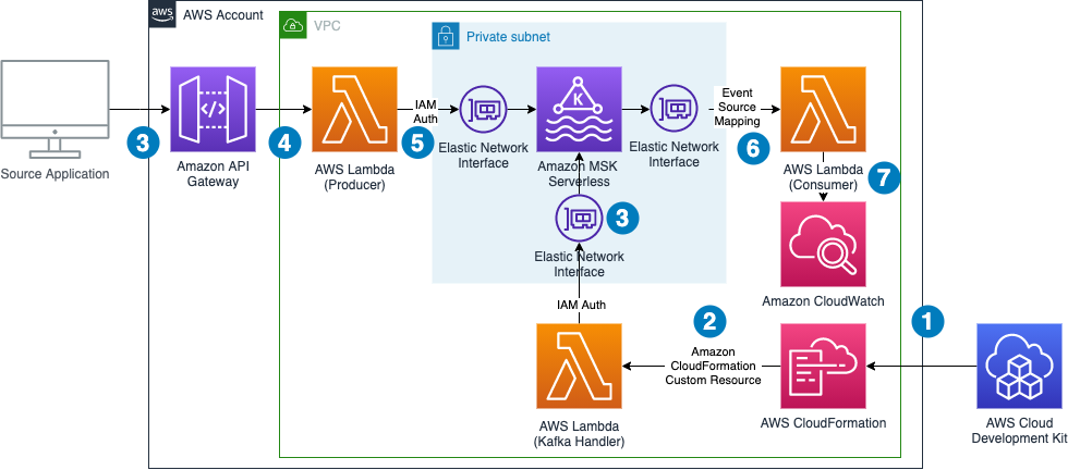
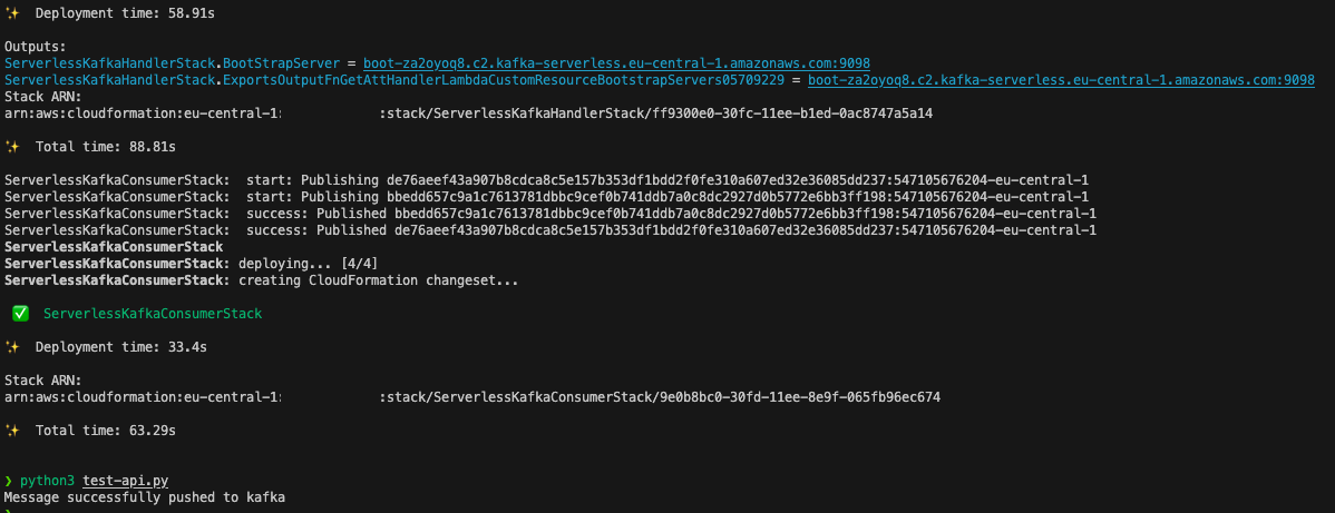
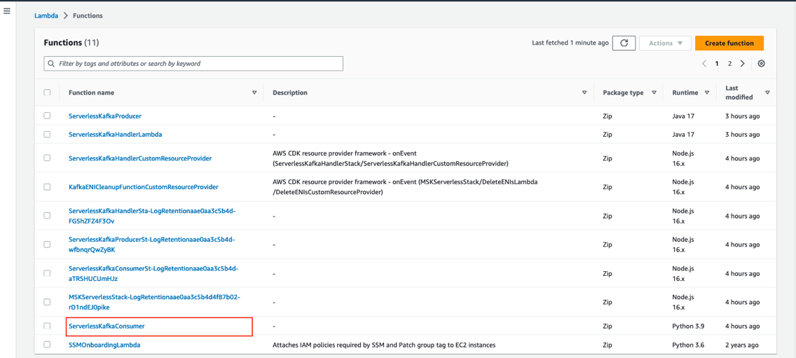
Build streaming data pipelines with Amazon MSK Serverless and IAM authentication

Post Syndicated from Marvin Gersho original https://aws.amazon.com/blogs/big-data/build-streaming-data-pipelines-with-amazon-msk-serverless-and-iam-authentication/

Currently, MSK Serverless only directly supports IAM for authentication using Java. This example shows how to use this mechanism. Additionally, it provides a pattern creating a proxy that can easily be integrated into solutions built in languages other than Java.

The rising trend in today’s tech landscape is the use of streaming data and event-oriented structures. They are being applied in numerous ways, including monitoring website traffic, tracking industrial Internet of Things (IoT) devices, analyzing video game player behavior, and managing data for cutting-edge analytics systems.

Apache Kafka, a top-tier open-source tool, is making waves in this domain. It’s widely adopted by numerous users for building fast and efficient data pipelines, analyzing streaming data, merging data from different sources, and supporting essential applications.

Amazon’s serverless Apache Kafka offering, Amazon Managed Streaming for Apache Kafka (Amazon MSK) Serverless, is attracting a lot of interest. It’s appreciated for its user-friendly approach, ability to scale automatically, and cost-saving benefits over other Kafka solutions. However, a hurdle encountered by many users is the requirement of MSK Serverless to use AWS Identity and Access Management (IAM) access control. At the time of writing, the Amazon MSK library for IAM is exclusive to Kafka libraries in Java, creating a challenge for users of other programming languages. In this post, we aim to address this issue and present how you can use Amazon API Gateway and AWS Lambda to navigate around this obstacle.

SASL/SCRAM authentication vs. IAM authentication

Compared to the traditional authentication methods like Salted Challenge Response Authentication Mechanism (SCRAM), the IAM extension into Apache Kafka through MSK Serverless provides a lot of benefits. Before we delve into those, it’s important to understand what SASL/SCRAM authentication is. Essentially, it’s a traditional method used to confirm a user’s identity before giving them access to a system. This process requires users or clients to provide a user name and password, which the system then cross-checks against stored credentials (for example, via AWS Secrets Manager) to decide whether or not access should be granted.

Compared to this approach, IAM simplifies permission management across AWS environments, enables the creation and strict enforcement of detailed permissions and policies, and uses temporary credentials rather than the typical user name and password authentication. Another benefit of using IAM is that you can use IAM for both authentication and authorization. If you use SASL/SCRAM, you have to additionally manage ACLs via a separate mechanism. In IAM, you can use the IAM policy attached to the IAM principal to define the fine-grained access control for that IAM principal. All of these improvements make the IAM integration a more efficient and secure solution for most use cases.

However, for applications not built in Java, utilizing MSK Serverless becomes tricky. The standard SASL/SCRAM authentication isn’t available, and non-Java Kafka libraries don’t have a way to use IAM access control. This calls for an alternative approach to connect to MSK Serverless clusters.

But there’s an alternative pattern. Without having to rewrite your existing application in Java, you can employ API Gateway and Lambda as a proxy in front of a cluster. They can handle API requests and relay them to Kafka topics instantly. API Gateway takes in producer requests and channels them to a Lambda function, written in Java using the Amazon MSK IAM library. It then communicates with the MSK Serverless Kafka topic using IAM access control. After the cluster receives the message, it can be further processed within the MSK Serverless setup.

You can also utilize Lambda on the consumer side of MSK Serverless topics, bypassing the Java requirement on the consumer side. You can do this by setting Amazon MSK as an event source for a Lambda function. When the Lambda function is triggered, the data sent to the function includes an array of records from the Kafka topic—no need for direct contact with Amazon MSK.

Solution overview

This example walks you through how to build a serverless real-time stream producer application using API Gateway and Lambda.

For testing, this post includes a sample AWS Cloud Development Kit (AWS CDK) application. This creates a demo environment, including an MSK Serverless cluster, three Lambda functions, and an API Gateway that consumes the messages from the Kafka topic.

The following diagram shows the architecture of the resulting application including its data flows.

The data flow contains the following steps:

  1. The infrastructure is defined in an AWS CDK application. By running this application, a set of AWS CloudFormation templates is created.
  2. AWS CloudFormation creates all infrastructure components, including a Lambda function that runs during the deployment process to create a topic in the MSK Serverless cluster and to retrieve the authentication endpoint needed for the producer Lambda function. On destruction of the CloudFormation stack, the same Lambda function gets triggered again to delete the topic from the cluster.
  3. An external application calls an API Gateway endpoint.
  4. API Gateway forwards the request to a Lambda function.
  5. The Lambda function acts as a Kafka producer and pushes the message to a Kafka topic using IAM authentication.
  6. The Lambda event source mapping mechanism triggers the Lambda consumer function and forwards the message to it.
  7. The Lambda consumer function logs the data to Amazon CloudWatch.

Note that we don’t need to worry about Availability Zones. MSK Serverless automatically replicates the data across multiple Availability Zones to ensure high availability of the data.

The demo additionally shows how to use Lambda Powertools for Java to streamline logging and tracing and the IAM authenticator for the simple authentication process outlined in the introduction.

The following sections take you through the steps to deploy, test, and observe the example application.

Prerequisites

The example has the following prerequisites:

  • An AWS account. If you haven’t signed up, complete the following steps:
  • The following software installed on your development machine, or use an AWS Cloud9 environment, which comes with all requirements preinstalled:
  • Appropriate AWS credentials for interacting with resources in your AWS account.

Deploy the solution

Complete the following steps to deploy the solution:

  1. Clone the project GitHub repository and change the directory to subfolder serverless-kafka-iac:
git clone https://github.com/aws-samples/apigateway-lambda-msk-serverless-integration
cd apigateway-lambda-msk-serverless-integration/serverless-kafka-iac
  1. Configure environment variables:
export CDK_DEFAULT_ACCOUNT=$(aws sts get-caller-identity --query 'Account' --output text)
export CDK_DEFAULT_REGION=$(aws configure get region)
  1. Prepare the virtual Python environment:
python3 -m venv .venv

source .venv/bin/activate

pip3 install -r requirements.txt
  1. Bootstrap your account for AWS CDK usage:
cdk bootstrap aws://$CDK_DEFAULT_ACCOUNT/$CDK_DEFAULT_REGION
  1. Run cdk synth to build the code and test the requirements (ensure docker daemon is running on your machine):
cdk synth
  1. Run cdk deploy to deploy the code to your AWS account:
cdk deploy --all

Test the solution

To test the solution, we generate messages for the Kafka topics by sending calls through the API Gateway from our development machine or AWS Cloud9 environment. We then go to the CloudWatch console to observe incoming messages in the log files of the Lambda consumer function.

  1. Open a terminal on your development machine to test the API with the Python script provided under /serverless_kafka_iac/test_api.py:
python3 test-api.py

  1. On the Lambda console, open the Lambda function named ServerlessKafkaConsumer.

  1. On the Monitor tab, choose View CloudWatch logs to access the logs of the Lambda function.

  1. Choose the latest log stream to access the log files of the last run.

You can review the log entry of the received Kafka messages in the log of the Lambda function.

Trace a request

All components integrate with AWS X-Ray. With AWS X-Ray, you can trace the entire application, which is useful to identify bottlenecks when load testing. You can also trace method runs at the Java method level.

Lambda Powertools for Java allows you to shortcut this process by adding the @Trace annotation to a method to see traces on the method level in X-Ray.

To trace a request end to end, complete the following steps:

  1. On the CloudWatch console, choose Service map in the navigation pane.
  2. Select a component to investigate (for example, the Lambda function where you deployed the Kafka producer).
  3. Choose View traces.

  1. Choose a single Lambda method invocation and investigate further at the Java method level.

Implement a Kafka producer in Lambda

Kafka natively supports Java. To stay open, cloud native, and without third-party dependencies, the producer is written in that language. Currently, the IAM authenticator is only available to Java. In this example, the Lambda handler receives a message from an API Gateway source and pushes this message to an MSK topic called messages.

Typically, Kafka producers are long-living and pushing a message to a Kafka topic is an asynchronous process. Because Lambda is ephemeral, you must enforce a full flush of a submitted message until the Lambda function ends by calling producer.flush():

// Copyright Amazon.com, Inc. or its affiliates. All Rights Reserved.
// SPDX-License-Identifier: MIT-0
package software.amazon.samples.kafka.lambda;
 
// This class is part of the AWS samples package and specifically deals with Kafka integration in a Lambda function.
// It serves as a simple API Gateway to Kafka Proxy, accepting requests and forwarding them to a Kafka topic.
public class SimpleApiGatewayKafkaProxy implements RequestHandler<APIGatewayProxyRequestEvent, APIGatewayProxyResponseEvent> {
 
    // Specifies the name of the Kafka topic where the messages will be sent
    public static final String TOPIC_NAME = "messages";
 
    // Logger instance for logging events of this class
    private static final Logger log = LogManager.getLogger(SimpleApiGatewayKafkaProxy.class);
    
    // Factory to create properties for Kafka Producer
    public KafkaProducerPropertiesFactory kafkaProducerProperties = new KafkaProducerPropertiesFactoryImpl();
    
    // Instance of KafkaProducer
    private KafkaProducer<String, String>[KT1]  producer;
 
    // Overridden method from the RequestHandler interface to handle incoming API Gateway proxy events
    @Override
    @Tracing
    @Logging(logEvent = true)
    public APIGatewayProxyResponseEvent handleRequest(APIGatewayProxyRequestEvent input, Context context) {
        
        // Creating a response object to send back 
        APIGatewayProxyResponseEvent response = createEmptyResponse();
        try {
            // Extracting the message from the request body
            String message = getMessageBody(input);
 
            // Create a Kafka producer
            KafkaProducer<String, String> producer = createProducer();
 
            // Creating a record with topic name, request ID as key and message as value 
            ProducerRecord<String, String> record = new ProducerRecord<String, String>(TOPIC_NAME, context.getAwsRequestId(), message);
 
            // Sending the record to Kafka topic and getting the metadata of the record
            Future<RecordMetadata>[KT2]  send = producer.send(record);
            producer.flush();
 
            // Retrieve metadata about the sent record
            RecordMetadata metadata = send.get();
 
            // Logging the partition where the message was sent
            log.info(String.format("Message was send to partition %s", metadata.partition()));
 
            // If the message was successfully sent, return a 200 status code
            return response.withStatusCode(200).withBody("Message successfully pushed to kafka");
        } catch (Exception e) {
            // In case of exception, log the error message and return a 500 status code
            log.error(e.getMessage(), e);
            return response.withBody(e.getMessage()).withStatusCode(500);
        }
    }
 
    // Creates a Kafka producer if it doesn't already exist
    @Tracing
    private KafkaProducer<String, String> createProducer() {
        if (producer == null) {
            log.info("Connecting to kafka cluster");
            producer = new KafkaProducer<String, String>(kafkaProducerProperties.getProducerProperties());
        }
        return producer;
    }
 
    // Extracts the message from the request body. If it's base64 encoded, it's decoded first.
    private String getMessageBody(APIGatewayProxyRequestEvent input) {
        String body = input.getBody();
 
        if (input.getIsBase64Encoded()) {
            body = decode(body);
        }
        return body;
    }
 
    // Creates an empty API Gateway proxy response event with predefined headers.
    private APIGatewayProxyResponseEvent createEmptyResponse() {
        Map<String, String> headers = new HashMap<>();
        headers.put("Content-Type", "application/json");
        headers.put("X-Custom-Header", "application/json");
        APIGatewayProxyResponseEvent response = new APIGatewayProxyResponseEvent().withHeaders(headers);
        return response;
    }
}

Connect to Amazon MSK using IAM authentication

This post uses IAM authentication to connect to the respective Kafka cluster. For information about how to configure the producer for connectivity, refer to IAM access control.

Because you configure the cluster via IAM, grant Connect and WriteData permissions to the producer so that it can push messages to Kafka:

{
    “Version”: “2012-10-17”,
    “Statement”: [
        {            
            “Effect”: “Allow”,
            “Action”: [
                “kafka-cluster:Connect”
            ],
            “Resource”: “arn:aws:kafka:region:account-id:cluster/cluster-name/cluster-uuid “
        }
    ]
}
 
 
{
    “Version”: “2012-10-17”,
    “Statement”: [
        {            
            “Effect”: “Allow”,
            “Action”: [
                “kafka-cluster:Connect”,
                “kafka-cluster: DescribeTopic”,
            ],
            “Resource”: “arn:aws:kafka:region:account-id:topic/cluster-name/cluster-uuid/topic-name“
        }
    ]
}

This shows the Kafka excerpt of the IAM policy, which must be applied to the Kafka producer. When using IAM authentication, be aware of the current limits of IAM Kafka authentication, which affect the number of concurrent connections and IAM requests for a producer. Refer to Amazon MSK quota and follow the recommendation for authentication backoff in the producer client:

        Map<String, String> configuration = Map.of(
                “key.serializer”, “org.apache.kafka.common.serialization.StringSerializer”,
                “value.serializer”, “org.apache.kafka.common.serialization.StringSerializer”,
                “bootstrap.servers”, getBootstrapServer(),
                “security.protocol”, “SASL_SSL”,
                “sasl.mechanism”, “AWS_MSK_IAM”,
                “sasl.jaas.config”, “software.amazon.msk.auth.iam.IAMLoginModule required;”,
                “sasl.client.callback.handler.class”,
				“software.amazon.msk.auth.iam.IAMClientCallbackHandler”,
                “connections.max.idle.ms”, “60”,
                “reconnect.backoff.ms”, “1000”
        );

Additional considerations

Each MSK Serverless cluster can handle 100 requests per second. To reduce IAM authentication requests from the Kafka producer, place it outside of the handler. For frequent calls, there is a chance that Lambda reuses the previously created class instance and only reruns the handler.

For bursting workloads with a high number of concurrent API Gateway requests, this can lead to dropped messages. Although this might be tolerable for some workloads, for others this might not be the case.

In these cases, you can extend the architecture with a buffering technology like Amazon Simple Queue Service (Amazon SQS) or Amazon Kinesis Data Streams between API Gateway and Lambda.

To reduce latency, reduce cold start times for Java by changing the tiered compilation level to 1, as described in Optimizing AWS Lambda function performance for Java. Provisioned concurrency ensures that polling Lambda functions don’t need to warm up before requests arrive.

Conclusion

In this post, we showed how to create a serverless integration Lambda function between API Gateway and MSK Serverless as a way to do IAM authentication when your producer is not written in Java. You also learned about the native integration of Lambda and Amazon MSK on the consumer side. Additionally, we showed how to deploy such an integration with the AWS CDK.

The general pattern is suitable for many use cases where you want to use IAM authentication but your producers or consumers are not written in Java, but you still want to take advantage of the benefits of MSK Serverless, like its ability to scale up and down with unpredictable or spikey workloads or its little to no operational overhead of running Apache Kafka.

You can also use MSK Serverless to reduce operational complexity by automating provisioning and the management of capacity needs, including the need to constantly monitor brokers and storage.

For more serverless learning resources, visit Serverless Land.

For more information on MSK Serverless, check out the following:


About the Authors

Philipp Klose is a Global Solutions Architect at AWS based in Munich. He works with enterprise FSI customers and helps them solve business problems by architecting serverless platforms. In this free time, Philipp spends time with his family and enjoys every geek hobby possible.

Daniel Wessendorf is a Global Solutions Architect at AWS based in Munich. He works with enterprise FSI customers and is primarily specialized in machine learning and data architectures. In his free time, he enjoys swimming, hiking, skiing, and spending quality time with his family.

Marvin Gersho is a Senior Solutions Architect at AWS based in New York City. He works with a wide range of startup customers. He previously worked for many years in engineering leadership and hands-on application development, and now focuses on helping customers architect secure and scalable workloads on AWS with a minimum of operational overhead. In his free time, Marvin enjoys cycling and strategy board games.

Nathan Lichtenstein is a Senior Solutions Architect at AWS based in New York City. Primarily working with startups, he ensures his customers build smart on AWS, delivering creative solutions to their complex technical challenges. Nathan has worked in cloud and network architecture in the media, financial services, and retail spaces. Outside of work, he can often be found at a Broadway theater.
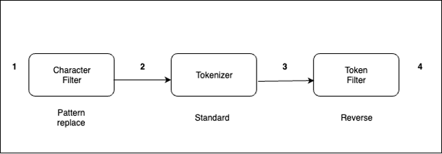
Use the reverse token filter to enable suffix matching queries in OpenSearch

Post Syndicated from Bharav Patel original https://aws.amazon.com/blogs/big-data/use-the-reverse-token-filter-to-enable-suffix-matching-queries-in-opensearch/

OpenSearch is an open-source RESTful search engine built on top of the Apache Lucene library. OpenSearch full-text search is fast, can give the result of complex queries within a fraction of a second. With OpenSearch, you can convert unstructured text into structured text using different text analyzers, tokenizers, and filters to improve search. OpenSearch uses a default analyzer, called the standard analyzer, which works well for most use cases out of the box. But for some use cases, it may not work best, and you need to use a specific analyzer.

In this post, we show how you can implement a suffix-based search. To find a document with the movie name “saving private ryan” for example, you can use the prefix “saving” with a prefix-based query. Occasionally, you also want to match suffixes as well, such as matching “Harry Potter Goblet of Fire” with the suffix “Fire” To do that, first reverse the string “eriF telboG rettoP yrraH” with the reverse token filter, then query for the prefix “eriF”.

Solution overview

Text analysis involves transforming unstructured text, such as the content of an email or a product description, into a structured format that is finely tuned for effective searching. An analyzer enables the implementation of full-text search using tokenization, which entails breaking down a text into smaller fragments known as tokens, with these tokens commonly representing individual words. To implement a reversed field search, the analyzer does the following.

The analyzer processes text in the following order:

  1. Use a character filter to replace - with _. For example, from “My Driving License Number Is 123-456-789” to “My Driving License Number Is 123_456_789.”
  2. The standard tokenizer splits texts into tokens. For example, from “My Driving License Number Is 123_456_789” to “[ my, driving, license, number, is, 123, 456, 789 ].”
  3. The reverse token filter reverses each token in a stream. For example, from [ my, driving, license, number, is, 123, 456, 789 ] to [ ym, gnivird, esnecil, rebmun, si, 321, 654, 987 ].

The standard analyzer (default analyzer) breaks down input strings into tokens based on word boundaries and removes most punctuation marks. For additional information about analyzers, refer Build-in analyzers.

Indexing and searching

Every document is a collection of fields, each having its own specific data type. When you create a mapping for your data, you create a mapping definition, which contains a list of fields that are pertinent to the document. To know more about index mappings refer to index mapping.

Let’s take the example of an analyzer with the reverse token filter applied on the text field.

  1. First, create an index with mappings as shown in the following code. The new field ‘reverse_title’ is derived from ‘title’ field for suffix search and original field ‘title’ will be used for normal search.
PUT movies
{
  "settings" : {
    "analysis" : {
      "analyzer" : {
        "whitespace_reverse" : {
          "tokenizer" : "whitespace",
          "filter" : ["reverse"]
        }
      }
    }
  },
  "mappings": {
    "properties": {
      "title": { 
        "type": "text",
        "analyzer": "standard",
        "copy_to": "reverse_title"
      },
      "reverse_title": {
        "type": "text",
        "analyzer": "whitespace_reverse"
      }
    }
  }
}

  1. Insert some documents into the index:
POST _bulk
{ "index" : { "_index" : "movies", "_id" : "1" } }
{ "title": "Harry Potter Goblet of Fire" }
{ "index" : { "_index" : "movies", "_id" : "2" } }
{ "title": "Lord of the rings" }
{ "index" : { "_index" : "movies", "_id" : "3" } }
{ "title": "Saving Private Ryan" }
  1. Run the following query to perform a suffix/reverse search on derived field ‘reverse_title’ for “Fire”:
GET movies/_search
{
  "query": {
    "prefix": {
      "reverse_title": {
        "value": "eriF"
      }
    }
  }
}

The following code shows our results:

   {
        "_index": "movies",
        "_id": "1",
        "_score": 1,
        "_source": {
          "title": "Harry Potter Goblet of Fire"
        }
      }
  1. For non-reverse search you can use original field ‘title’.
GET movies/_search
{
  "query": {
    "match": {
      "title": "Fire"
    }
  }
}

The following code shows our result.

{
        "_index": "movies",
        "_id": "1",
        "_score": 0.2876821,
        "_source": {
          "title": "Harry Potter Goblet of Fire"
        }
}

The query returns a document with the movie name “Harry Potter Goblet of Fire”.
If you’re curious to know how search works at high level, refer to A query, or There and Back Again.

Conclusion

In this post, you walked through how text analysis works in OpenSearch and how to implement suffix-based search using a reverse token filter effectively.

If you have feedback about this post, submit your comments in the comments section.


About the Authors

Bharav Patel is a Specialist Solution Architect, Analytics at Amazon Web Services. He primarily works on Amazon OpenSearch Service and helps customers with key concepts and design principles of running OpenSearch workloads on the cloud. Bharav likes to explore new places and try out different cuisines.

Stored procedure enhancements in Amazon Redshift

Post Syndicated from Milind Oke original https://aws.amazon.com/blogs/big-data/stored-procedure-enhancements-in-amazon-redshift/

Amazon Redshift is a fully managed, petabyte-scale data warehouse service in the cloud. With Amazon Redshift, you can analyze all your data to derive holistic insights about your business and your customers. It supports stored procedures where prepared SQL code is saved and the code can be reused over and over again.

Stored procedures are commonly used to encapsulate logic for data transformation, data validation, and business-specific logic. By combining multiple SQL steps into a stored procedure, you can create reusable code blocks that can run together as a single transaction or multiple individual transactions. You can also schedule stored procedures to automate data processing on Amazon Redshift. For more information, refer to Bringing your stored procedures to Amazon Redshift.

In the Redshift stored procedure default atomic transaction mode, a call to a Redshift stored procedure will create its own transaction when the call starts or is part of the existing transaction if an explicit transaction is opened before the stored procedure is called. All the statements inside a procedure behave as if they are in a single transaction block that ends when the stored procedure call finishes. A nested call to another procedure is treated like any other SQL statement and operates within the context of the same transaction as the caller. Statements for TRUNCATE, COMMIT, and ROLLBACK and the exception handling block with arbitrary SQL statements close the current transaction and start a new transaction implicitly. This behavior can cause challenges in migration to Amazon Redshift from other systems like Teradata.

In this post, we discuss the enhancements to Amazon Redshift stored procedures for non-atomic transaction mode. This mode provides enhanced transaction controls that enable you to automatically commit the statements inside the stored procedure.

Non-atomic transaction mode

The new non-atomic transaction mode feature provides three enhancements on stored procedures in Amazon Redshift:

  • Unless the DML or DDL statements are part of an explicit open transaction, each statement in the stored procedure will run in its own implicit transaction and a new transaction will be opened to handle following statements. If an explicit transaction is opened, then all subsequent statements are run and remain un-committed until an explicit transaction control command (COMMIT or ROLLBACK) is run to end the transaction.
  • Amazon Redshift will not re-raise the exception after the exception handler statements are complete. Therefore, a new RAISE statement without any INFO or EXCEPTION has been provided to re-throw the exception caught by the exception handling block. This RAISE statement without any INFO or EXCEPTION will only be allowed in the exception handling block.
  • Also, the new START TRANSACTION statement begins an explicit transaction inside the non-atomic transaction mode stored procedure. Use the existing transaction control command (COMMIT or ROLLBACK) to end the explicitly started transaction.
    • Amazon Redshift does not support sub-transactions so if there is already an open transaction, then calling this statement again will do nothing, and no error is raised.
    • If an explicit transaction is still open when the nonatomic transaction mode stored procedure call ends, then the explicit transaction remains open until a transaction control command is run in the session.
    • If the session disconnects before running a transaction control command, the whole transaction is automatically rolled back.

Additional restrictions

Some restrictions have also been introduced for Redshift stored procedures:

  • For nesting stored procedure calls, all the procedures must be created in the same transaction mode, no matter if it’s in atomic (default) transaction mode or the new non-atomic transaction mode
  • You can’t nest stored procedures across the two transaction modes (atomic and non-atomic)
  • You can’t set the SECURITY DEFINER option or SET configuration_parameter option for non-atomic transaction mode stored procedures

Impact to cursors

Cursors in non-atomic transaction mode stored procedures will behave differently compared to the default atomic transaction mode:

  • Cursor statements will need an explicit transaction block before beginning the cursor to ensure that each iteration of the cursor loop is not auto-committed.
  • To return a cursor from non-atomic transaction mode stored procedure, you will need an explicit transaction block before beginning the cursor. Otherwise, the cursor will be closed when the SQL statement inside the loop is automatically committed.

Advantages

The following are key advantages of this feature from a user perspective:

  • It provides the capability to lift and shift Teradata stored procedures to run in Teradata session mode. This helps in seamless migrations from traditional data warehouses like Teradata and SQL Server.
  • It enables Amazon Redshift to provide more flexible operations inside of stored procedures when encountering errors and exceptions. Amazon Redshift can now preserve previous action’s state before reaching an exception.

Syntax

The new optional keyword NONATOMIC has been added to the stored procedure definition syntax, as shown in the following code:

CREATE [ OR REPLACE ] PROCEDURE sp_procedure_name
( [ [ argname ] [ argmode ] argtype [, ...] ] )
[ NONATOMIC ]
AS $$
procedure_body
$$ LANGUAGE plpgsql

This optional keyword creates the stored procedure under the non-atomic transaction mode. If you don’t specify the keyword, then the default atomic mode will be the transaction mode when creating the stored procedure.

NONATOMIC means each DML and DDL statement in the procedure will be implicitly committed.

Without non-atomic mode, the procedure will create its own transaction when the call starts or be part of the existing transaction if an explicit transaction is opened before it is called. Every statement within the stored procedure will belong to this one transaction.

Example of NONATOMIC mode

Let’s consider the customer contact table custcontacts, which stores customer primary and secondary contact phone numbers:

CREATE table custcontacts(
custid int4 not null,
primaryphone char(10),
secondaryphone char(10));

We insert three sample customer records with no contact values:

INSERT INTO custcontacts VALUES (101, 'xxxxxxxxxx', 'xxxxxxxxxx');
INSERT INTO custcontacts VALUES (102, 'xxxxxxxxxx', 'xxxxxxxxxx');
INSERT INTO custcontacts VALUES (103, 'xxxxxxxxxx', 'xxxxxxxxxx');

You need to create a stored procedure to update the primary and secondary phone numbers. The requirement is not to roll back updates to the primary contact number if updates to the secondary contact number fail for some reason.

You can achieve this by creating the stored procedure with the NONATOMIC keyword. The NONATOMIC keyword ensures that each statement in the stored procedure runs in its own implicit transaction block. Therefore, if the UPDATE statement for the secondary phone fails, then it won’t roll back the data update made to the primary phone. See the following code:

CREATE PROCEDURE sp_update_custcontacts(cid int4,pphone char(15),sphone char(15)) NONATOMIC AS
$$
BEGIN
UPDATE custcontacts SET primaryphone=pphone WHERE custid=cid;
UPDATE custcontacts SET secondaryphone=sphone WHERE custid=cid;
END;
$$
LANGUAGE plpgsql;

Now let’s call the stored procedure passing the secondary phone number with more than 10 digits, which will fail in the secondaryphone UPDATE statement due to incorrect length:

call sp_update_custcontacts(101,'1234567890','345443345324');

The preceding procedure call will update the primary phone number successfully. The secondary phone number update fails. However, the primaryphone update will not roll back because it ran in its own implicit transaction block due to the NONATOMIC clause in the stored procedure definition.

select * from custcontacts;

custcontacts | primaryphone | secondaryphone
-------------+---------------+---------------
101 | 1234567890 | XXXXXXXXXX
102 | XXXXXXXXXX | XXXXXXXXXX
103 | XXXXXXXXXX | XXXXXXXXXX

Exception handling in NONATOMIC mode

Exceptions are handled in stored procedures differently based on the atomic or non-atomic mode:

  • Atomic (default) – Exceptions are always re-raised
  • Non-atomic – Exceptions are handled and you can choose to re-raise or not

Let’s continue with the previous example to illustrate exception handling in non-atomic mode.

Create the following table to log exceptions raised by stored procedures:

CREATE TABLE procedure_log
(log_timestamp timestamp, procedure_name varchar(100), error_message varchar(255));

Now update the sp_update_custcontacts() procedure to handle exceptions. Note that we’re adding an EXCEPTION block in the procedure definition. It inserts a record in the procedure_log table in the event of an exception.

CREATE OR REPLACE PROCEDURE sp_update_custcontacts(cid int4,pphone char(15),sphone char(15)) NONATOMIC AS
$$
BEGIN
UPDATE custcontacts SET primaryphone=pphone WHERE custid=cid;
UPDATE custcontacts SET secondaryphone=sphone WHERE custid=cid;
EXCEPTION
WHEN OTHERS THEN
INSERT INTO procedure_log VALUES (getdate(), 'sp_update_custcontacts', sqlerrm);
END;
$$
LANGUAGE plpgsql;

Now create one more stored procedure, which will call the preceding procedure. It also has an EXCEPTION block and inserts a record in the procedure_log table in the event of an exception.

CREATE PROCEDURE sp_update_customer() NONATOMIC AS
$$
BEGIN
-- Let us assume you have additional staments here to update other fields. For this example, ommitted them for simplifiction.
-- Nested call to update contacts
call sp_update_custcontacts(101,'1234567890','345443345324');
EXCEPTION
WHEN OTHERS THEN
INSERT INTO procedure_log VALUES (getdate(), 'sp_update_customer', sqlerrm);
END;
$$
LANGUAGE plpgsql;

Let’s call the parent procedure we created:

call sp_update_customer();

This in turn will call the sp_update_custcontacts() procedure. The inner procedure sp_update_custcontacts() will fail because we’re updating the secondary phone with an invalid value. The control will enter the EXCEPTION block of the sp_update_custcontacts() procedure and make an insert into the procedure_log table.

However, it will not re-raise the exception in non-atomic mode. Therefore, the parent procedure sp_update_customer() will not get the exception passed from the sp_update_custcontacts() procedure. The control will not enter the EXCEPTION block of the sp_update_customer() procedure.

If you query the procedure_log table, you will see an entry only for the error handled by the sp_update_custcontacts() procedure:

select * from procedure_log;

Procedure Log Output

Now redefine the sp_update_custcontacts() procedure with the RAISE statement:

CREATE PROCEDURE sp_update_custcontacts(cid int4,pphone char(15),sphone char(15)) NONATOMIC AS
$$
BEGIN
UPDATE custcontacts SET primaryphone=pphone WHERE custid=cid;
UPDATE custcontacts SET secondaryphone=sphone WHERE custid=cid;
EXCEPTION
WHEN OTHERS THEN
INSERT INTO procedure_log VALUES (getdate(), 'sp_update_custcontacts', sqlerrm);
RAISE;
END;
$$
LANGUAGE plpgsql;

Let’s call the parent stored procedure sp_update_customer() again:

call sp_update_customer();

Now the inner procedure sp_update_custcontacts() will re-raise the exception to the parent procedure sp_update_customer() after handling the exception in its own EXCEPTION block. Then the control will reach the EXCEPTION block in the parent procedure and insert another record into the procedure_log table.

If you query the procedure_log table now, you will see two entries: one by the inner procedure sp_update_custcontacts() and another by the parent procedure sp_update_customer(). This demonstrates that the RAISE statement in the inner procedure re-raised the exception.

select * from procedure_log;

Procedure log output

Explicit START TRANSACTION statement in non-atomic mode

You can issue a START TRANSACTION statement to begin a transaction block inside the stored procedure. It will open a new transaction inside the stored procedure. For examples, refer to Nonatomic mode stored procedure transaction management.

Conclusion

In this post, we discussed the enhancements to Redshift stored procedures for non-atomic transaction mode, which provides enhanced transaction controls to enable you to automatically commit the statements inside the stored procedure. This mode also enables easier migration to Amazon Redshift from other systems like Teradata. Try out these enhancements and let us know your experience in comments.


About the Authors

Milind Oke is a Data Warehouse Specialist Solutions Architect based out of New York. He has been building data warehouse solutions for over 15 years and specializes in Amazon Redshift.

Satesh Sonti is a Sr. Analytics Specialist Solutions Architect based out of Atlanta, specialized in building enterprise data platforms, data warehousing, and analytics solutions. He has over 17 years of experience in building data assets and leading complex data platform programs for banking and insurance clients across the globe.

Kiran Chinta is a Software Development Manager at Amazon Redshift. He leads a strong team in query processing, SQL language, data security, and performance. Kiran is passionate about delivering products that seamlessly integrate with customers’ business applications with the right ease of use and performance. In his spare time, he enjoys reading and playing tennis.

Huichen Liu is a software development engineer on the Amazon Redshift query processing team. She focuses on query optimization, statistics and SQL language features. In her spare time, she enjoys hiking and photography.
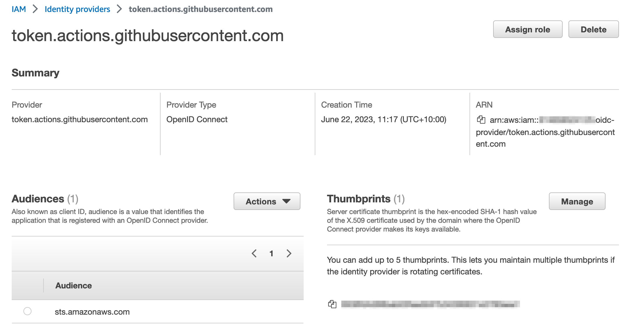
Validate IAM policies by using IAM Policy Validator for AWS CloudFormation and GitHub Actions

Post Syndicated from Mitch Beaumont original https://aws.amazon.com/blogs/security/validate-iam-policies-by-using-iam-policy-validator-for-aws-cloudformation-and-github-actions/

In this blog post, I’ll show you how to automate the validation of AWS Identity and Access Management (IAM) policies by using a combination of the IAM Policy Validator for AWS CloudFormation (cfn-policy-validator) and GitHub Actions. Policy validation is an approach that is designed to minimize the deployment of unwanted IAM identity-based and resource-based policies to your Amazon Web Services (AWS) environments.

With GitHub Actions, you can automate, customize, and run software development workflows directly within a repository. Workflows are defined using YAML and are stored alongside your code. I’ll discuss the specifics of how you can set up and use GitHub actions within a repository in the sections that follow.

The cfn-policy-validator tool is a command-line tool that takes an AWS CloudFormation template, finds and parses the IAM policies that are attached to IAM roles, users, groups, and resources, and then runs the policies through IAM Access Analyzer policy checks. Implementing IAM policy validation checks at the time of code check-in helps shift security to the left (closer to the developer) and shortens the time between when developers commit code and when they get feedback on their work.

Let’s walk through an example that checks the policies that are attached to an IAM role in a CloudFormation template. In this example, the cfn-policy-validator tool will find that the trust policy attached to the IAM role allows the role to be assumed by external principals. This configuration could lead to unintended access to your resources and data, which is a security risk.

Prerequisites

To complete this example, you will need the following:

  1. A GitHub account
  2. An AWS account, and an identity within that account that has permissions to create the IAM roles and resources used in this example

Step 1: Create a repository that will host the CloudFormation template to be validated

To begin with, you need to create a GitHub repository to host the CloudFormation template that is going to be validated by the cfn-policy-validator tool.

To create a repository:

  1. Open a browser and go to https://github.com.
  2. In the upper-right corner of the page, in the drop-down menu, choose New repository. For Repository name, enter a short, memorable name for your repository.
  3. (Optional) Add a description of your repository.
  4. Choose either the option Public (the repository is accessible to everyone on the internet) or Private (the repository is accessible only to people access is explicitly shared with).
  5. Choose Initialize this repository with: Add a README file.
  6. Choose Create repository. Make a note of the repository’s name.

Step 2: Clone the repository locally

Now that the repository has been created, clone it locally and add a CloudFormation template.

To clone the repository locally and add a CloudFormation template:

  1. Open the command-line tool of your choice.
  2. Use the following command to clone the new repository locally. Make sure to replace <GitHubOrg> and <RepositoryName> with your own values.
    git clone [email protected]:<GitHubOrg>/<RepositoryName>.git

  3. Change in to the directory that contains the locally-cloned repository.
    cd <RepositoryName>

    Now that the repository is locally cloned, populate the locally-cloned repository with the following sample CloudFormation template. This template creates a single IAM role that allows a principal to assume the role to perform the S3:GetObject action.

  4. Use the following command to create the sample CloudFormation template file.

    WARNING: This sample role and policy should not be used in production. Using a wildcard in the principal element of a role’s trust policy would allow any IAM principal in any account to assume the role.

    cat << EOF > sample-role.yaml
    
    AWSTemplateFormatVersion: "2010-09-09"
    Description: Base stack to create a simple role
    Resources:
      SampleIamRole:
        Type: AWS::IAM::Role
        Properties:
          AssumeRolePolicyDocument:
            Statement:
              - Effect: Allow
                Principal:
                  AWS: "*"
                Action: ["sts:AssumeRole"]
          Path: /      
          Policies:
            - PolicyName: root
              PolicyDocument:
                Version: 2012-10-17
                Statement:
                  - Resource: "*"
                    Effect: Allow
                    Action:
                      - s3:GetObject
    EOF

Notice that AssumeRolePolicyDocument refers to a trust policy that includes a wildcard value in the principal element. This means that the role could potentially be assumed by an external identity, and that’s a risk you want to know about.

Step 3: Vend temporary AWS credentials for GitHub Actions workflows

In order for the cfn-policy-validator tool that’s running in the GitHub Actions workflow to use the IAM Access Analyzer API, the GitHub Actions workflow needs a set of temporary AWS credentials. The AWS Credentials for GitHub Actions action helps address this requirement. This action implements the AWS SDK credential resolution chain and exports environment variables for other actions to use in a workflow. Environment variable exports are detected by the cfn-policy-validator tool.

AWS Credentials for GitHub Actions supports four methods for fetching credentials from AWS, but the recommended approach is to use GitHub’s OpenID Connect (OIDC) provider in conjunction with a configured IAM identity provider endpoint.

To configure an IAM identity provider endpoint for use in conjunction with GitHub’s OIDC provider:

  1. Open the AWS Management Console and navigate to IAM.
  2. In the left-hand menu, choose Identity providers, and then choose Add provider.
  3. For Provider type, choose OpenID Connect.
  4. For Provider URL, enter
    https://token.actions.githubusercontent.com
  5. Choose Get thumbprint.
  6. For Audiences, enter sts.amazonaws.com
  7. Choose Add provider to complete the setup.

At this point, make a note of the OIDC provider name. You’ll need this information in the next step.

After it’s configured, the IAM identity provider endpoint should look similar to the following:

Figure 1: IAM Identity provider details

Figure 1: IAM Identity provider details

Step 4: Create an IAM role with permissions to call the IAM Access Analyzer API

In this step, you will create an IAM role that can be assumed by the GitHub Actions workflow and that provides the necessary permissions to run the cfn-policy-validator tool.

To create the IAM role:

  1. In the IAM console, in the left-hand menu, choose Roles, and then choose Create role.
  2. For Trust entity type, choose Web identity.
  3. In the Provider list, choose the new GitHub OIDC provider that you created in the earlier step. For Audience, select sts.amazonaws.com from the list.
  4. Choose Next.
  5. On the Add permission page, choose Create policy.
  6. Choose JSON, and enter the following policy:
    
        "Version": "2012-10-17",
        "Statement": [
            {
                "Effect": "Allow",
                "Action": [
                  "iam:GetPolicy",
                  "iam:GetPolicyVersion",
                  "access-analyzer:ListAnalyzers",
                  "access-analyzer:ValidatePolicy",
                  "access-analyzer:CreateAccessPreview",
                  "access-analyzer:GetAccessPreview",
                  "access-analyzer:ListAccessPreviewFindings",
                  "access-analyzer:CreateAnalyzer",
                  "s3:ListAllMyBuckets",
                  "cloudformation:ListExports",
                  "ssm:GetParameter"
                ],
                "Resource": "*"
            },
            {
              "Effect": "Allow",
              "Action": "iam:CreateServiceLinkedRole",
              "Resource": "*",
              "Condition": {
                "StringEquals": {
                  "iam:AWSServiceName": "access-analyzer.amazonaws.com"
                }
              }
            } 
        ]
    }

  7. After you’ve attached the new policy, choose Next.

    Note: For a full explanation of each of these actions and a CloudFormation template example that you can use to create this role, see the IAM Policy Validator for AWS CloudFormation GitHub project.

  8. Give the role a name, and scroll down to look at Step 1: Select trusted entities.

    The default policy you just created allows GitHub Actions from organizations or repositories outside of your control to assume the role. To align with the IAM best practice of granting least privilege, let’s scope it down further to only allow a specific GitHub organization and the repository that you created earlier to assume it.

  9. Replace the policy to look like the following, but don’t forget to replace {AWSAccountID}, {GitHubOrg} and {RepositoryName} with your own values.
    {
        "Version": "2012-10-17",
        "Statement": [
            {
                "Effect": "Allow",
                "Principal": {
                    "Federated": "arn:aws:iam::{AWSAccountID}:oidc-provider/token.actions.githubusercontent.com"
                },
                "Action": "sts:AssumeRoleWithWebIdentity",
                "Condition": {
                    "StringEquals": {
                        "token.actions.githubusercontent.com:aud": "sts.amazonaws.com"
                    },
                    "StringLike": {
                        "token.actions.githubusercontent.com:sub": "repo:${GitHubOrg}/${RepositoryName}:*"
                    }
                }
            }
        ]
    }

For information on best practices for configuring a role for the GitHub OIDC provider, see Creating a role for web identity or OpenID Connect Federation (console).

Checkpoint

At this point, you’ve created and configured the following resources:

  • A GitHub repository that has been locally cloned and filled with a sample CloudFormation template.
  • An IAM identity provider endpoint for use in conjunction with GitHub’s OIDC provider.
  • A role that can be assumed by GitHub actions, and a set of associated permissions that allow the role to make requests to IAM Access Analyzer to validate policies.

Step 5: Create a definition for the GitHub Actions workflow

The workflow runs steps on hosted runners. For this example, we are going to use Ubuntu as the operating system for the hosted runners. The workflow runs the following steps on the runner:

  1. The workflow checks out the CloudFormation template by using the community actions/checkout action.
  2. The workflow then uses the aws-actions/configure-aws-credentials GitHub action to request a set of credentials through the IAM identity provider endpoint and the IAM role that you created earlier.
  3. The workflow installs the cfn-policy-validator tool by using the python package manager, PIP.
  4. The workflow runs a validation against the CloudFormation template by using the cfn-policy-validator tool.

The workflow is defined in a YAML document. In order for GitHub Actions to pick up the workflow, you need to place the definition file in a specific location within the repository: .github/workflows/main.yml. Note the “.” prefix in the directory name, indicating that this is a hidden directory.

To create the workflow:

  1. Use the following command to create the folder structure within the locally cloned repository:
    mkdir -p .github/workflows

  2. Create the sample workflow definition file in the .github/workflows directory. Make sure to replace <AWSAccountID> and <AWSRegion> with your own information.
    cat << EOF > .github/workflows/main.yml
    name: cfn-policy-validator-workflow
    
    on: push
    
    permissions:
      id-token: write
      contents: read
    
    jobs: 
      cfn-iam-policy-validation: 
        name: iam-policy-validation
        runs-on: ubuntu-latest
        steps:
          - name: Checkout code
            uses: actions/checkout@v3
    
          - name: Configure AWS Credentials
            uses: aws-actions/configure-aws-credentials@v2
            with:
              role-to-assume: arn:aws:iam::<AWSAccountID>:role/github-actions-access-analyzer-role
              aws-region: <AWSRegion>
              role-session-name: GitHubSessionName
            
          - name: Install cfn-policy-validator
            run: pip install cfn-policy-validator
    
          - name: Validate templates
            run: cfn-policy-validator validate --template-path ./sample-role-test.yaml --region <AWSRegion>
    EOF
    

Step 6: Test the setup

Now that everything has been set up and configured, it’s time to test.

To test the workflow and validate the IAM policy:

  1. Add and commit the changes to the local repository.
    git add .
    git commit -m ‘added sample cloudformation template and workflow definition’

  2. Push the local changes to the remote GitHub repository.
    git push

    After the changes are pushed to the remote repository, go back to https://github.com and open the repository that you created earlier. In the top-right corner of the repository window, there is a small orange indicator, as shown in Figure 2. This shows that your GitHub Actions workflow is running.

    Figure 2: GitHub repository window with the orange workflow indicator

    Figure 2: GitHub repository window with the orange workflow indicator

    Because the sample CloudFormation template used a wildcard value “*” in the principal element of the policy as described in the section Step 2: Clone the repository locally, the orange indicator turns to a red x (shown in Figure 3), which signals that something failed in the workflow.

    Figure 3: GitHub repository window with the red cross workflow indicator

    Figure 3: GitHub repository window with the red cross workflow indicator

  3. Choose the red x to see more information about the workflow’s status, as shown in Figure 4.
    Figure 4: Pop-up displayed after choosing the workflow indicator

    Figure 4: Pop-up displayed after choosing the workflow indicator

  4. Choose Details to review the workflow logs.

    In this example, the Validate templates step in the workflow has failed. A closer inspection shows that there is a blocking finding with the CloudFormation template. As shown in Figure 5, the finding is labelled as EXTERNAL_PRINCIPAL and has a description of Trust policy allows access from external principals.

    Figure 5: Details logs from the workflow showing the blocking finding

    Figure 5: Details logs from the workflow showing the blocking finding

    To remediate this blocking finding, you need to update the principal element of the trust policy to include a principal from your AWS account (considered a zone of trust). The resources and principals within your account comprises of the zone of trust for the cfn-policy-validator tool. In the initial version of sample-role.yaml, the IAM roles trust policy used a wildcard in the Principal element. This allowed principals outside of your control to assume the associated role, which caused the cfn-policy-validator tool to generate a blocking finding.

    In this case, the intent is that principals within the current AWS account (zone of trust) should be able to assume this role. To achieve this result, replace the wildcard value with the account principal by following the remaining steps.

  5. Open sample-role.yaml by using your preferred text editor, such as nano.
    nano sample-role.yaml

    Replace the wildcard value in the principal element with the account principal arn:aws:iam::<AccountID>:root. Make sure to replace <AWSAccountID> with your own AWS account ID.

    AWSTemplateFormatVersion: "2010-09-09"
    Description: Base stack to create a simple role
    Resources:
      SampleIamRole:
        Type: AWS::IAM::Role
        Properties:
          AssumeRolePolicyDocument:
            Statement:
              - Effect: Allow
                Principal:
                  AWS: "arn:aws:iam::<AccountID>:root"
                Action: ["sts:AssumeRole"]
          Path: /      
          Policies:
            - PolicyName: root
              PolicyDocument:
                Version: 2012-10-17
                Statement:
                  - Resource: "*"
                    Effect: Allow
                    Action:
                      - s3:GetObject

  6. Add the updated file, commit the changes, and push the updates to the remote GitHub repository.
    git add sample-role.yaml
    git commit -m ‘replacing wildcard principal with account principal’
    git push

After the changes have been pushed to the remote repository, go back to https://github.com and open the repository. The orange indicator in the top right of the window should change to a green tick (check mark), as shown in Figure 6.

Figure 6: GitHub repository window with the green tick workflow indicator

Figure 6: GitHub repository window with the green tick workflow indicator

This indicates that no blocking findings were identified, as shown in Figure 7.

Figure 7: Detailed logs from the workflow showing no more blocking findings

Figure 7: Detailed logs from the workflow showing no more blocking findings

Conclusion

In this post, I showed you how to automate IAM policy validation by using GitHub Actions and the IAM Policy Validator for CloudFormation. Although the example was a simple one, it demonstrates the benefits of automating security testing at the start of the development lifecycle. This is often referred to as shifting security left. Identifying misconfigurations early and automatically supports an iterative, fail-fast model of continuous development and testing. Ultimately, this enables teams to make security an inherent part of a system’s design and architecture and can speed up product development workflows.

In addition to the example I covered today, IAM Policy Validator for CloudFormation can validate IAM policies by using a range of IAM Access Analyzer policy checks. For more information about these policy checks, see Access Analyzer reference policy checks.

 
If you have feedback about this post, submit comments in the Comments section below. If you have questions about this post, contact AWS Support.

Want more AWS Security news? Follow us on Twitter.

Mitch Beaumont

Mitch Beaumont

Mitch is a Principal Solutions Architect for Amazon Web Services, based in Sydney, Australia. Mitch works with some of Australia’s largest financial services customers, helping them to continually raise the security bar for the products and features that they build and ship. Outside of work, Mitch enjoys spending time with his family, photography, and surfing.

Generate machine learning insights for Amazon Security Lake data using Amazon SageMaker

Post Syndicated from Jonathan Nguyen original https://aws.amazon.com/blogs/security/generate-machine-learning-insights-for-amazon-security-lake-data-using-amazon-sagemaker/

Amazon Security Lake automatically centralizes the collection of security-related logs and events from integrated AWS and third-party services. With the increasing amount of security data available, it can be challenging knowing what data to focus on and which tools to use. You can use native AWS services such as Amazon QuickSight, Amazon OpenSearch, and Amazon SageMaker Studio to visualize, analyze, and interactively identify different areas of interest to focus on, and prioritize efforts to increase your AWS security posture.

In this post, we go over how to generate machine learning insights for Security Lake using SageMaker Studio. SageMaker Studio is a web integrated development environment (IDE) for machine learning that provides tools for data scientists to prepare, build, train, and deploy machine learning models. With this solution, you can quickly deploy a base set of Python notebooks focusing on AWS Security Hub findings in Security Lake, which can also be expanded to incorporate other AWS sources or custom data sources in Security Lake. After you’ve run the notebooks, you can use the results to help you identify and focus on areas of interest related to security within your AWS environment. As a result, you might implement additional guardrails or create custom detectors to alert on suspicious activity.

Prerequisites

  1. Specify a delegated administrator account to manage the Security Lake configuration for all member accounts within your organization.
  2. Security Lake has been enabled in the delegated administrator AWS account.
  3. As part of the solution in this post, we focus on Security Hub as a data source. AWS Security Hub must be enabled for your AWS Organizations. When enabling Security Lake, select All log and event sources to include AWS Security Hub findings.
  4. Configure subscriber query access to Security Lake. Security Lake uses AWS Lake Formation cross-account table sharing to support subscriber query access. Accept the resource share request in the subscriber AWS account in AWS Resource Access Manager (AWS RAM). Subscribers with query access can query the data that Security Lake collects. These subscribers query Lake Formation tables in an Amazon Simple Storage Service (Amazon S3) bucket with Security Lake data using services such as Amazon Athena.

Solution overview

Figure 1 that follows depicts the architecture of the solution.

Figure 1 SageMaker machine learning insights architecture for Security Lake

Figure 1 SageMaker machine learning insights architecture for Security Lake

The deployment builds the architecture by completing the following steps:

  1. A Security Lake is set up in an AWS account with supported log sources — such as Amazon VPC Flow Logs, AWS Security Hub, AWS CloudTrail, and Amazon Route53 — configured.
  2. Subscriber query access is created from the Security Lake AWS account to a subscriber AWS account.

    Note: See Prerequisite #4 for more information.

  3. The AWS RAM resource share request must be accepted in the subscriber AWS account where this solution is deployed.

    Note: See Prerequisite #4 for more information.

  4. A resource link database in Lake Formation is created in the subscriber AWS account and grants access for the Athena tables in the Security Lake AWS account.
  5. VPC is provisioned for SageMaker with IGW, NAT GW, and VPC endpoints for the AWS services used in the solution. IGW and NAT are required to install external open-source packages.
  6. A SageMaker Domain for SageMaker Studio is created in VPCOnly mode with a single SageMaker user profile that is tied to a dedicated AWS Identity and Access Management (IAM) role.
  7. A dedicated IAM role is created to restrict access to create and access the presigned URL for the SageMaker Domain from a specific CIDR for accessing the SageMaker notebook.
  8. An AWS CodeCommit repository containing Python notebooks is used for the AI and ML workflow by the SageMaker user-profile.
  9. An Athena workgroup is created for the Security Lake queries with an S3 bucket for output location (access logging configured for the output bucket).

Deploy the solution

You can deploy the SageMaker solution by using either the AWS Management Console or the AWS Cloud Development Kit (AWS CDK).

Option 1: Deploy the solution with AWS CloudFormation using the console

Use the console to sign in to your subscriber AWS account and then choose the Launch Stack button to open the AWS CloudFormation console pre-loaded with the template for this solution. It takes approximately 10 minutes for the CloudFormation stack to complete.

Select this image to open a link that starts building the CloudFormation stack

Option 2: Deploy the solution by using the AWS CDK

You can find the latest code for the SageMaker solution in the SageMaker machine learning insights GitHub repository, where you can also contribute to the sample code. For instructions and more information on using the AWS CDK, see Get Started with AWS CDK.

To deploy the solution by using the AWS CDK

  1. To build the app when navigating to the project’s root folder, use the following commands:
    npm install -g aws-cdk-lib
    npm install

  2. Update IAM_role_assumption_for_sagemaker_presigned_url and security_lake_aws_account default values in source/lib/sagemaker_domain.ts with their respective appropriate values.
  3. Run the following commands in your terminal while authenticated in your subscriber AWS account. Be sure to replace <INSERT_AWS_ACCOUNT> with your account number and replace <INSERT_REGION> with the AWS Region that you want the solution deployed to.
    cdk bootstrap aws://<INSERT_AWS_ACCOUNT>/<INSERT_REGION>
    cdk deploy

Post deployment steps

Now that you’ve deployed the SageMaker solution, you must grant the SageMaker user profile in the subscriber AWS account query access to your Security Lake. You can Grant permission for the SageMaker user profile to Security Lake in Lake Formation in the subscriber AWS account.

Grant permission to the Security Lake database

  1. Copy the SageMaker user-profile Amazon resource name (ARN) arn:aws:iam::<account-id>:role/sagemaker-user-profile-for-security-lake
  2. Go to Lake Formation in the console.
  3. Select the amazon_security_lake_glue_db_us_east_1 database.
  4. From the Actions Dropdown, select Grant.
  5. In Grant Data Permissions, select SAML Users and Groups.
  6. Paste the SageMaker user profile ARN from Step 1.
  7. In Database Permissions, select Describe and then Grant.

Grant permission to Security Lake – Security Hub table

  1. Copy the SageMaker user-profile ARN arn:aws:iam:<account-id>:role/sagemaker-user-profile-for-security-lake
  2. Go to Lake Formation in the console.
  3. Select the amazon_security_lake_glue_db_us_east_1 database.
  4. Choose View Tables.
  5. Select the amazon_security_lake_table_us_east_1_sh_findings_1_0 table.
  6. From Actions Dropdown, select Grant.
  7. In Grant Data Permissions, select SAML Users and Groups.
  8. Paste the SageMaker user-profile ARN from Step 1.
  9. In Table Permissions, select Describe and then Grant.

Launch your SageMaker Studio application

Now that you have granted permissions for a SageMaker user-profile, we can move on to launching the SageMaker application associated to that user-profile.

  1. Navigate to the SageMaker Studio domain in the console.
  2. Select the SageMaker domain security-lake-ml-insights-<account-id>.
  3. Select the SageMaker user profile sagemaker-user-profile-for-security-lake.
  4. Select the Launch drop-down and select Studio
    Figure 2 SageMaker domain user-profile AWS console screen

    Figure 2: SageMaker domain user-profile AWS console screen

Clone Python notebooks

You’ll work primarily in the SageMaker user profile to create a data-science app to work in. As part of the solution deployment, we’ve created Python notebooks in CodeCommit that you will need to clone.

To clone the Python notebooks

  1. Navigate to CloudFormation in the console.
  2. In the Stacks section, select the SageMakerDomainStack.
  3. Select to the Outputs tab/
  4. Copy the value for sagemakernotebookmlinsightsrepositoryURL. (For example: https://git-codecommit.us-east-1.amazonaws.com/v1/repos/sagemaker_ml_insights_repo)
  5. Go back to your SageMaker app.
  6. In Studio, in the left sidebar, choose the Git icon (identified by a diamond with two branches), then choose Clone a Repository.
    Figure 3 SageMaker clone CodeCommit repository

    Figure 3: SageMaker clone CodeCommit repository

  7. Paste the CodeCommit repository link from Step 4 under the Git repository URL (git). After you paste the URL, select Clone “https://git-codecommit.us-east-1.amazonaws.com/v1/repos/sagemaker_ml_insights_repo”, then select Clone.

    NOTE: If you don’t select from the auto-populated drop-down, SageMaker won’t be able to clone the repository.

    Figure 4 SageMaker clone CodeCommit URL

    Figure 4: SageMaker clone CodeCommit URL

Generating machine learning insights using SageMaker Studio

You’ve successfully pulled the base set of Python notebooks into your SageMaker app and they can be accessed at sagemaker_ml_insights_repo/notebooks/tsat/. The notebooks provide you with a starting point for running machine learning analysis using Security Lake data. These notebooks can be expanded to existing native or custom data sources being sent to Security Lake.

Figure 5: SageMaker cloned Python notebooks

Figure 5: SageMaker cloned Python notebooks

Notebook #1 – Environment setup

The 0.0-tsat-environ-setup notebook handles the installation of the required libraries and dependencies needed for the subsequent notebooks within this blog. For our notebooks, we use an open-source Python library called Kats, which is a lightweight, generalizable framework to perform time series analysis.

  1. Select the 0.0-tsat-environ-setup.ipynb notebook for the environment setup.

    Note: If you have already provisioned a kernel, you can skip steps 2 and 3.

  2. In the right-hand corner, select No Kernel
  3. In the Set up notebook environment pop-up, leave the defaults and choose Select.
    Figure 6 SageMaker application environment settings

    Figure 6: SageMaker application environment settings

  4. After the kernel has successfully started, choose the Terminal icon to open the image terminal.
    Figure 7: SageMaker application terminal

    Figure 7: SageMaker application terminal

  5. To install open-source packages from https instead of http, you must update the sources.list file. After the terminal opens, send the following commands:
    cd /etc/apt
    sed -i 's/http:/https:/g' sources.list

  6. Go back to the 0.0-tsat-environ-setup.ipynb notebook and select the Run drop-down and select Run All Cells. Alternatively, you can run each cell independently, but it’s not required. Grab a coffee! This step will take about 10 minutes.

    IMPORTANT: If you complete the installation out of order or update the requirements.txt file, you might not be able to successfully install Kats and you will need to rebuild your environment by using a net-new SageMaker user profile.

  7. After installing all the prerequisites, check the Kats version to determine if it was successfully installed.
    Figure 8: Kats installation verification

    Figure 8: Kats installation verification

  8. Install PyAthena (Python DB API client for Amazon Athena) which is used to query your data in Security Lake.

You’ve successfully set up the SageMaker app environment! You can now load the appropriate dataset and create a time series.

Notebook #2 – Load data

The 0.1-load-data notebook establishes the Athena connection to query data in Security Lake and creates the resulting time series dataset. The time series dataset will be used for subsequent notebooks to identify trends, outliers, and change points.

  1. Select the 0.1-load-data.ipynb notebook.
  2. If you deployed the solution outside of us-east-1, update the con details to the appropriate Region. In this example, we’re focusing on Security Hub data within Security Lake. If you want to change the underlying data source, you can update the TABLE value.
    Figure 9: SageMaker notebook load Security Lake data settings

    Figure 9: SageMaker notebook load Security Lake data settings

  3. In the Query section, there’s an Athena query to pull specific data from Security Hub, this can be expanded as needed to a subset or can include all products within Security Hub. The query below pulls Security Hub information after 01:00:00 1/1/2022 from the products listed in productname.
    Figure 10: SageMaker notebook Athena query

    Figure 10: SageMaker notebook Athena query

  4. After the values have been updated, you can create your time series dataset. For this notebook, we recommend running each cell individually instead of running all cells at once so you can get a bit more familiar with the process. Select the first cell and choose the Run icon.
    Figure 11: SageMaker run Python notebook code

    Figure 11: SageMaker run Python notebook code

  5. Follow the same process as Step 4 for the subsequent cells.

    Note: If you encounter any issues with querying the table, make sure you completed the post-deployment step for Grant permission to Security Lake – Security Hub table.

You’ve successfully loaded your data and created a timeseries! You can now move on to generating machine learning insights from your timeseries.

Notebook #3 – Trend detector

The 1.1-trend-detector.ipynb notebook handles trend detection in your data. Trend represents a directional change in the level of a time series. This directional change can be either upward (increase in level) or downward (decrease in level). Trend detection helps detect a change while ignoring the noise from natural variability. Each environment is different, and trends help us identify where to look more closely to determine why a trend is positive or negative.

  1. Select 1.1-trend-detector.ipynb notebook for trend detection.
  2. Slopes are created to identify the relationship between x (time) and y (counts).
    Figure 12: SageMaker notebook slope view

    Figure 12: SageMaker notebook slope view

  3. If the counts are increasing with time, then it’s considered a positive slope and the reverse is considered a negative slope. A positive slope isn’t necessarily a good thing because in an ideal state we would expect counts of a finding type to come down with time.
    Figure 13: SageMaker notebook trend view

    Figure 13: SageMaker notebook trend view

  4. Now you can plot the top five positive and negative trends to identify the top movers.
    Figure 14: SageMaker notebook trend results view

    Figure 14: SageMaker notebook trend results view

Notebook #4 – Outlier detection

The 1.2-outlier-detection.ipynb notebook handles outlier detection. This notebook does a seasonal decomposition of the input time series, with additive or multiplicative decomposition as specified (default is additive). It uses a residual time series by either removing only trend or both trend and seasonality if the seasonality is strong. The intent is to discover useful, abnormal, and irregular patterns within data sets, allowing you to pinpoint areas of interest.

  1. To start, it detects points in the residual that are over 5 times the inter-quartile range.
  2. Inter-quartile range (IQR) is the difference between the seventy-fifth and twenty-fifth percentiles of residuals or the spread of data within the middle two quartiles of the entire dataset. IQR is useful in detecting the presence of outliers by looking at values that might lie outside of the middle two quartiles.
  3. The IQR multiplier controls the sensitivity of the range and decision of identifying outliers. By using a larger value for the iqr_mult_thresh parameter in OutlierDetector, outliers would be considered data points, while a smaller value would identify data points as outliers.

    Note: If you don’t have enough data, decrease iqr_mult_thresh to a lower value (for example iqr_mult_thresh=3).

    Figure 15: SageMaker notebook outlier setting

    Figure 15: SageMaker notebook outlier setting

  4. Along with outlier detection plots, investigation SQL will be displayed as well, which can help with further investigation of the outliers.

    In the diagram that follows, you can see that there are several outliers in the number of findings, related to failed AWS Firewall Manager policies, which have been identified by the vertical red lines within the line graph. These are outliers because they deviate from the normal behavior and number of findings on a day-to-day basis. When you see outliers, you can look at the resources that might have caused an unusual increase in Firewall Manager policy findings. Depending on the findings, it could be related to an overly permissive or noncompliant security group or a misconfigured AWS WAF rule group.

    Figure 16: SageMaker notebook outlier results view

    Figure 16: SageMaker notebook outlier results view

Notebook #5 – Change point detection

The 1.3-changepoint-detector.ipynb notebook handles the change point detection. Change point detection is a method to detect changes in a time series that persist over time, such as a change in the mean value. To detect a baseline to identify when several changes might have occurred from that point. Change points occur when there’s an increase or decrease to the average number of findings within a data set.

  1. Along with identifying change points within the data set, the investigation SQL is generated to further investigate the specific change point if applicable.

    In the following diagram, you can see there’s a change point decrease after July 27, 2022, with confidence of 99.9 percent. It’s important to note that change points differ from outliers, which are sudden changes in the data set observed. This diagram means there was some change in the environment that resulted in an overall decrease in the number of findings for S3 buckets with block public access being disabled. The change could be the result of an update to the CI/CD pipelines provisioning S3 buckets or automation to enable all S3 buckets to block public access. Conversely, if you saw a change point that resulted in an increase, it could mean that there was a change that resulted in a larger number of S3 buckets with a block public access configuration consistently being disabled.

    Figure 17: SageMaker changepoint detector view

    Figure 17: SageMaker changepoint detector view

By now, you should be familiar with the set up and deployment for SageMaker Studio and how you can use Python notebooks to generate machine learning insights for your Security Lake data. You can take what you’ve learned and start to curate specific datasets and data sources within Security Lake, create a time series, detect trends, and identify outliers and change points. By doing so, you can answer a variety of security-related questions such as:

  • CloudTrail

    Is there a large volume of Amazon S3 download or copy commands to an external resource? Are you seeing a large volume of S3 delete object commands? Is it possible there’s a ransomware event going on?

  • VPC Flow Logs

    Is there an increase in the number of requests from your VPC to external IPs? Is there an increase in the number of requests from your VPC to your on-premises CIDR? Is there a possibility of internal or external data exfiltration occurring?

  • Route53

    Which resources are making DNS requests that they haven’t typically made within the last 30–45 days? When did it start? Is there a potential command and control session occurring on an Amazon Elastic Compute Cloud (Amazon EC2) instance?

It’s important to note that this isn’t a solution to replace Amazon GuardDuty, which uses foundational data sources to detect communication with known malicious domains and IP addresses and identify anomalous behavior, or Amazon Detective, which provides customers with prebuilt data aggregations, summaries, and visualizations to help security teams conduct faster and more effective investigations. One of the main benefits of using Security Lake and SageMaker Studio is the ability to interactively create and tailor machine learning insights specific to your AWS environment and workloads.

Clean up

If you deployed the SageMaker machine learning insights solution by using the Launch Stack button in the AWS Management Console or the CloudFormation template sagemaker_ml_insights_cfn, do the following to clean up:

  1. In the CloudFormation console for the account and Region where you deployed the solution, choose the SageMakerML stack.
  2. Choose the option to Delete the stack.

If you deployed the solution by using the AWS CDK, run the command cdk destroy.

Conclusion

Amazon Security Lake gives you the ability to normalize and centrally store your security data from various log sources to help you analyze, visualize, and correlate appropriate security logs. You can then use this data to increase your overall security posture by implementing additional security guardrails or take appropriate remediation actions within your AWS environment.

In this blog post, you learned how you can use SageMaker to generate machine learning insights for your Security Hub findings in Security Lake. Although the example solution focuses on a single data source within Security Lake, you can expand the notebooks to incorporate other native or custom data sources in Security Lake.

There are many different use-cases for Security Lake that can be tailored to fit your AWS environment. Take a look at this blog post to learn how you can ingest, transform and deliver Security Lake data to Amazon OpenSearch to help your security operations team quickly analyze security data within your AWS environment. In supported Regions, new Security Lake account holders can try the service free for 15 days and gain access to its features.

 
If you have feedback about this post, submit comments in the Comments section below. If you have questions about this post, contact AWS Support.

Want more AWS Security news? Follow us on Twitter.

Jonathan Nguyen

Jonathan Nguyen

Jonathan is a Principal Security Architect at AWS. His background is in AWS security, with a focus on threat detection and incident response. He helps enterprise customers develop a comprehensive AWS security strategy, deploy security solutions at scale, and train customers on AWS security best practices.

Madhunika Reddy Mikkili

Madhunika Reddy Mikkili

Madhunika is a Data and Machine Learning Engineer with the AWS Professional Services Shared Delivery Team. She is passionate about helping customers achieve their goals through the use of data and machine learning insights. Outside of work, she loves traveling and spending time with family and friends.

How we designed Cedar to be intuitive to use, fast, and safe

Post Syndicated from Emina Torlak original https://aws.amazon.com/blogs/security/how-we-designed-cedar-to-be-intuitive-to-use-fast-and-safe/

This post is a deep dive into the design of Cedar, an open source language for writing and evaluating authorization policies. Using Cedar, you can control access to your application’s resources in a modular and reusable way. You write Cedar policies that express your application’s permissions, and the application uses Cedar’s authorization engine to decide which access requests to allow. This decouples access control from the application logic, letting you write, update, audit, and reuse authorization policies independently of application code.

Cedar’s authorization engine is built to a high standard of performance and correctness. Application developers report typical authorization latencies of less than 1 ms, even with hundreds of policies. The resulting authorization decision — Allow or Deny — is provably correct, thanks to the use of verification-guided development. This high standard means your application can use Cedar with confidence, just like Amazon Web Services (AWS) does as part of the Amazon Verified Permissions and AWS Verified Access services.

Cedar’s design is based on three core tenets: usability, speed, and safety. Cedar policies are intuitive to read because they’re defined using your application’s vocabulary—for example, photos organized into albums for a photo-sharing application. Cedar’s policy structure reflects common authorization use cases and enables fast evaluation. Cedar’s semantics are intuitive and safer by default: policies combine to allow or deny access according to rules you already know from AWS Identity and Access Management (IAM).

This post shows how Cedar’s authorization semantics, data model, and policy syntax work together to make the Cedar language intuitive to use, fast, and safe. We cover each of these in turn and highlight how their design reflects our tenets.

The Cedar authorization semantics: Default deny, forbid wins, no ordering

We show how Cedar works on an example application for sharing photos, called PhotoFlash, illustrated in Figure 1.

Figure 1: An example PhotoFlash account. User Jane has two photos, four albums, and three user groups

Figure 1: An example PhotoFlash account. User Jane has two photos, four albums, and three user groups

PhotoFlash lets users like Jane upload photos to the cloud, tag them, and organize them into albums. Jane can also share photos with others, for example, letting her friends view photos in her trips album. PhotoFlash provides a point-and-click interface for users to share access, and then stores the resulting permissions as Cedar policies.

When a user attempts to perform an action on a resource (for example, view a photo), PhotoFlash calls the Cedar authorization engine to determine whether access is allowed. The authorizer evaluates the stored policies against the request and application-specific data (such as a photo’s tags) and returns Allow or Deny. If it returns Allow, PhotoFlash proceeds with the action. If it returns Deny, PhotoFlash reports that the action is not permitted.

Let’s look at some policies and see how Cedar evaluates them to authorize requests safely and simply.

Default deny

To let Jane’s friends view photos in her trips album, PhotoFlash generates and stores the following Cedar permit policy:

// Policy A: Jane's friends can view photos in Jane's trips album.
permit(
  principal in Group::"jane/friends", 
  action == Action::"viewPhoto",
  resource in Album::"jane/trips");

Cedar policies define who (the principal) can do what (the action) on what asset (the resource). This policy allows the principal (a PhotoFlash User) in Jane’s friends group to view the resources (a Photo) in Jane’s trips album.

Cedar’s authorizer grants access only if a request satisfies a specific permit policy. This semantics is default deny: Requests that don’t satisfy any permit policy are denied.

Given only our example Policy A, the authorizer will allow Alice to view Jane’s flower.jpg photo. Alice’s request satisfies Policy A because Alice is one of Jane’s friends (see Figure 1). But the authorizer will deny John’s request to view this photo. That’s because John isn’t one of Jane’s friends, and there is no other permit that grants John access to Jane’s photos.

Forbid wins

While PhotoFlash allows individual users to choose their own permissions, it also enforces system-wide security rules.

For example, PhotoFlash wants to prevent users from performing actions on resources that are owned by someone else and tagged as private. If a user (Jane) accidentally permits someone else (Alice) to view a private photo (receipt.jpg), PhotoFlash wants to override the user-defined permission and deny the request.

In Cedar, such guardrails are expressed as forbid policies:

// Policy B: Users can't perform any actions on private resources they don't own.
forbid(principal, action, resource)
when {
  resource.tags.contains("private") &&
  !(resource in principal.account)
};

This PhotoFlash policy says that a principal is forbidden from taking an action on a resource when the resource is tagged as private and isn’t contained in the principal’s account.

Cedar’s authorizer makes sure that forbids override permits. If a request satisfies a forbid policy, it’s denied regardless of what permissions are satisfied.

For example, the authorizer will deny Alice’s request to view Jane’s receipt.jpg photo. This request satisfies Policy A because Alice is one of Jane’s friends. But it also satisfies the guardrail in Policy B because the photo is tagged as private. The guardrail wins, and the request is denied.

No ordering

Cedar’s authorization decisions are independent of the order the policies are evaluated in. Whether the authorizer evaluates Policy A first and then Policy B, or the other way around, doesn’t matter. As you’ll see later, the Cedar language design ensures that policies can be evaluated in any order to reach the same authorization decision. To understand the combined meaning of multiple Cedar policies, you need only remember that access is allowed if the request satisfies a permit policy and there are no applicable forbid policies.

Safe by default and intuitive

We’ve proved (using automated reasoning) that Cedar’s authorizer satisfies the default deny, forbids override permits, and order independence properties. These properties help make Cedar’s behavior safe by default and intuitive. Amazon IAM has the same properties. Cedar builds on more than a decade of IAM experience by formalizing and enforcing these properties as parts of its design.

Now that we’ve seen how Cedar authorizes requests, let’s look at how its data model and syntax support writing policies that are quick to read and evaluate.

The Cedar data model: entities with attributes, arranged in a hierarchy

Cedar policies are defined in terms of a vocabulary specific to your application. For example, PhotoFlash organizes photos into albums and users into groups while a task management application organizes tasks into lists. You reflect this vocabulary into Cedar’s data model, which organizes entities into a hierarchy. Entities correspond to objects within your application, such as photos and users. The hierarchy reflects grouping of entities, such as nesting of photos into albums. Think of it as a directed-acyclic graph. Figure 2 shows the entity hierarchy for PhotoFlash that matches Figure 1.

Figure 2: An example hierarchy for PhotoFlash, matching the illustration in Figure 1

Figure 2: An example hierarchy for PhotoFlash, matching the illustration in Figure 1

Entities are stored objects that serve as principals, resources, and actions in Cedar policies. Policies refer to these objects using entity references, such as Album::”jane/art”.

Policies use the in operator to check if the hierarchy relates two entities. For example, Photo::”flower.jpg” in Account::”jane” is true for the hierarchy in Figure 2, but Photo::”flower.jpg” in Album::”jane/conference” is not. PhotoFlash can persist the entity hierarchy in a dedicated entity store, or compute the relevant parts as needed for an authorization request.

Each entity also has a record that maps named attributes to values. An attribute stores a Cedar value: an entity reference, record, string, 64-bit integer, boolean, or a set of values. For example, Photo::”flower.jpg” has attributes describing the photo’s metadata, such as tags, which is a set of strings, and raw, which is an entity reference to another Photo. Cedar supports a small collection of operators that can be applied to values; these operators are carefully chosen to enable efficient evaluation.

Built-in support for role and attribute-based access control

If the concepts you’ve seen so far seem familiar, that’s not surprising. Cedar’s data model is designed to allow you to implement time-tested access control models, including role-based and attribute-based access control (RBAC and ABAC). The entity hierarchy and the in operator support RBAC-style roles as groups, while entity records and the . operator let you express ABAC-style permissions using per-object attributes.

The Cedar syntax: Structured, loop-free, and stateless

Cedar uses a simple, structured syntax for writing policies. This structure makes Cedar policies simple to understand and fast to authorize at scale. Let’s see how by taking a closer look at Cedar’s syntax.

Structure for readability and scalable authorization

Figure 3 illustrates the structure of Cedar policies: an effect and scope, optionally followed by one or more conditions.

The effect of a policy is to either permit or forbid access. The scope can use equality (==) or membership (in) constraints to restrict the principals, actions, and resources to which the policy applies. Policy conditions are expressions that further restrict when the policy applies.

This structure makes policies straightforward to read and understand: The scope expresses an RBAC rule, and the conditions express ABAC rules. For example, PhotoFlash Policy A has no conditions and expresses a single RBAC rule. Policy B has an open (unconstrained) scope and expresses a single ABAC rule. A quick glance is enough to see if a policy is just an RBAC rule, just an ABAC rule, or a mix of both.

Figure 3: Cedar policy structure, illustrated on PhotoFlash Policy A and B

Figure 3: Cedar policy structure, illustrated on PhotoFlash Policy A and B

Scopes also enable scalable authorization for large policy stores through policy slicing. This is a property of Cedar that lets applications authorize a request against a subset of stored policies, supporting real-time decisions even for stores with thousands of policies. With slicing, an application needs to pass a policy to the authorizer only when the request’s principal and resource are descendants of the principal and resource entities specified in the policy’s scope. For example, PhotoFlash needs to include Policy A only for requests that involve the descendants of Group::”jane/friends” and Album::”jane/trips”. But Policy B must be included for all requests because of its open scope.

No loops or state for fast evaluation and intuitive decisions

Policy conditions are Boolean-valued expressions. The Cedar expression language has a familiar syntax that includes if-then-else expressions, short-circuiting Boolean operators (!, &&, ||), and basic operations on Cedar values. Notably, there is no way to express looping or to change the application state (for example, mutate an attribute).

Cedar excludes loops to bound authorization latency. With no loops or costly built-in operators, Cedar policies terminate in O(n2) steps in the worst case (when conditions contain certain set operations), or O(n) in the common case.

Cedar also excludes stateful operations for performance and understandability. Since policies can’t change the application state, their evaluation can be parallelized for better performance, and you can reason about them in any order to see what accesses are allowed.

Learn more

In this post, we explored how Cedar’s design supports intuitive, fast, and safe authorization. With Cedar, your application’s access control rules become standalone policies that are clear, auditable, and reusable. You enforce these policies by calling Cedar’s authorizer to decide quickly and safely which requests are allowed. To learn more, see how to use Cedar to secure your app, and how we built Cedar to a high standard of assurance. You can also visit the Cedar website and blog, try it out in the Cedar playground, and join us on Cedar’s Slack channel.

 
If you have feedback about this post, submit comments in the Comments section below. If you have questions about this post, contact AWS Support.

Want more AWS Security news? Follow us on Twitter.

Emina Torlak

Emina Torlak

Emina is a Senior Principal Applied Scientist at Amazon Web Services and an Associate Professor at the University of Washington. Her research aims to help developers build better software more easily. She develops languages and tools for program verification and synthesis. Emina co-leads the development of Cedar.

Amazon CloudWatch metrics for Amazon OpenSearch Service storage and shard skew health

Post Syndicated from Nikhil Agarwal original https://aws.amazon.com/blogs/big-data/amazon-cloudwatch-metrics-for-amazon-opensearch-service-storage-and-shard-skew-health/

Amazon OpenSearch Service is a managed service that makes it easy to deploy, operate, and scale OpenSearch clusters in AWS to perform interactive log analytics, real-time application monitoring, website search, and more. OpenSearch is an open source, distributed search and analytics suite.

When working with OpenSearch Service, shard strategy is key. Shards distribute your workload across the data nodes of your cluster. When creating an index, you tell OpenSearch Service how many primary shards to create and how many replicas to create of each shard. The primary shards are independent partitions of the full dataset. OpenSearch Service automatically distributes your data across the primary shards in an index. Our recommendation is to use two replicas for your index. For example, if you set your index’s shard count to three primary shards and two replicas, you will have a total of nine shards. Properly configured indexes can help boost overall domain performance, whereas a misconfigured index will lead to storage and performance skew.

OpenSearch Service distributes the shards in your indexes to the data nodes in your domain, ensuring that no primary shard and its replicas are placed on the same node. The data for the shards are stored in the node’s storage. If your indexes (and therefore their shards) are very different sizes, the storage used on the data nodes in the domain will be unequal, or skewed. Storage skew leads to uneven memory and CPU utilization, intermittent and uneven latency, and uneven queueing and rejecting of requests. Therefore, it’s important to configure and maintain indexes such that shards can be distributed evenly across the data nodes of your cluster.

In this post, we explore how to deploy Amazon CloudWatch metrics using an AWS CloudFormation template to monitor an OpenSearch Service domain’s storage and shard skew. This solution uses an AWS Lambda function to extract storage and shard distribution metadata from your OpenSearch Service domain, calculates the level of skew, and then pushes this information to CloudWatch metrics so that you can easily monitor, alert, and respond.

Solution overview

The solution and associated resources are available for you to deploy into your own AWS account as a CloudFormation template. The template deploys the following resources:

  • An AWS Identity and Access Management (IAM) role for the Lambda function called OpensearchSkewMetricsLambdaRole. This allows write access to CloudWatch metrics and access to the CloudWatch log group and OpenSearch APIs.
  • An AWS Lambda function called Opensearch-SkewMetricsPublisher-py.
  • An Amazon CloudWatch log group for the Lambda function called /aws/lambda/Opensearch-skewmetrics-publisher-py.
  • An Amazon EventBridge rule for the Lambda function called EventRuleForOSSkew.
  • The following CloudWatch metrics for the Lambda function:
    • aws_/<region-name>/<MetricIdentifier>/_storagemetric
    • aws_/<region-name>/<MetricIdentifier>/_shardmetric

Prerequisites

For this walkthrough, you should have the following prerequisites:

  • An AWS account.
  • An OpenSearch Service domain.
  • This post requires you to add a Lambda role to the OpenSearch Service domain’s security configuration access policy. If your domain is using fine-grained access control, then you need to follow the steps as described in the section Mapping roles to users to enable access for the newly deployed Lambda execution role to the domain after deploying the CloudFormation template.

Deploy the CloudFormation template

To deploy the CloudFormation template, complete the following steps:

  1. Log in to your AWS account.
  2. Select the Region where you’re running your OpenSearch Service domain.
  3. To launch your CloudFormation stack, choose Launch Stack
  4. For Stack name, enter a name for the stack (maximum length 30 characters).
  5. For MetricIdentifier, enter a unique identifier that will help you identify the custom CloudWatch metrics for your domain.
  6. For OpensearchDomainURL, enter the domain endpoint that you are monitoring.
  7. Choose Next.
  8. Select I acknowledge that AWS CloudFormation might create IAM resources, then choose Create stack.
  9. Wait for the stack creation to complete.
  10. On the Lambda console, choose Functions in the navigation pane.
  11. Choose the Lambda function called Opensearch-SkewMetricsPublisher-py-<stackname>.
  12. In the Code section, choose Test.
  13. Keep the default values for the test event and run a quick test.

Make sure to grant the Lambda execution role permission to the OpenSearch Service domain’s resource-based policy, if you are using one. If fine-grained access control is enabled on the domain, then follow the steps in Mapping roles to users (as mentioned in the prerequisites) to allow the Lambda function to read from the domain in read-only access.

The Lambda function that sends OpenSearch domain metrics to CloudWatch is set to a default frequency of 1 day. You can change this configuration to monitor the domain at the required granularity by updating the event schedule for the rule deployed by the CloudFormation stack on the EventBridge console. Note that if the frequency is set to 1 minute, this will trigger the Lambda function every minute and will increase the Lambda cost.

This solution uses the cat/allocation API, which provides the number of data nodes in the domain along with each data node’s number of shards and storage usage attributes. For further details on domain storage and shard skew, refer to Node shard and storage skew. The Lambda function processes and sorts each data node’s storage and shard skew from the average value. Any data node’s skew above 10% from the average is generally considered to be significantly skewed. This will start to impact CPU, network, and disk bandwidth usage because the nodes with the highest storage utilization tend to be the resource-strained nodes, whereas nodes with less than 10% usage represent underutilized capacity.

Refer to Demystifying Elasticsearch shard allocation for details related to shard size and shard count strategy. In general, we recommend keeping shard sizes between 10–30 GB for workloads where search latency is a key performance objective and 30–50 GB for write-heavy workloads. For shard count, we recommend maintaining index shard counts that are divisible by the data node count. For additional details, refer to Sizing Amazon OpenSearch Service domains and Shard strategy.

View skew metrics in CloudWatch

After you run this solution in your account, it will create two CloudWatch metrics for monitoring. To access these CloudWatch metrics, use the following steps:

  1. On the CloudWatch console, under Metrics in the navigation pane, choose All metrics.
  2. Choose Browse and select Custom namespaces. You should see two custom metrics ending with _storageworkspace and _shardworkspace, respectively.
  3. Choose either of the custom metrics and then select NodeID.
  4. On the list of node IDs, select all the nodes displayed in the list, and the graph will be plotted automatically.

You can hover the mouse over the plotted lines to see the node skew information.

The following screenshots show examples of how the CloudWatch metrics will appear on the console.

The storage skew metrics will be similar to the following screenshot. Storage skew metrics shows the domain storage skew. If you hover over the graph, it shows the node list with available nodes in the domain. This list is sorted by the storage size (largest to smallest). The Lambda function will periodically post the latest storage skew results.

The shard skew metrics will be similar to the following screenshot. Shard skew metrics show the domain shard skew. If you hover over the graph, it shows the node list with available nodes in the domain. This list is sorted by the shard size (largest to smallest). The Lambda function will periodically post the latest storage skew results.

Storage skew occurs when one or more nodes within the domain has significantly more storage than other nodes. The CloudWatch metric will show higher deviation of storage usage for these nodes vs. other nodes. Similarly, shard skew occurs when one or more nodes has significantly more shards than others nodes. The CloudWatch metric will show higher deviation for these nodes vs. other nodes in the domain. When the domain storage or shard skew is detected, you can raise a support case to work with the AWS team for remediation actions. See How do I rebalance the uneven shard distribution in my Amazon OpenSearch Service cluster for information on how to take remediation actions to configure your domain shard strategy for optimal performance.

Costs

The cost associated with using this solution would be minimal, around few cents per month since it generates CloudWatch metrics. The solution also runs Lambda code, and in this case the Lambda functions make API calls. For pricing details, refer to Amazon CloudWatch Pricing and AWS Lambda Pricing.

Clean up

If you decide that you no longer want to keep the Lambda function and associated resources, you can navigate to the AWS CloudFormation console, choose the stack, and choose Delete.

If you want to add the CloudWatch skew monitor metrics mechanism back in at any point, you can create the stack again from the CloudFormation template.

Conclusion

You can use this solution to get a better understanding of your OpenSearch Service domain’s storage and shard skew to improve its performance and possibly lower the cost of operating your domain. See Use Elasticsearch’s _rollover API For efficient storage distribution for more details related to shard allocation and efficient storage distribution strategy.


About the authors

Nikhil Agarwal is Sr. Technical Manager with Amazon Web Services. He is passionate about helping customers achieve operational excellence in their cloud journey and working activity on technical solutions. He is also AI/ML enthusiastic and deep dives into customer’s ML-specific use cases. Outside of work, he enjoys traveling with family and exploring different gadgets.

Karthik Chemudupati is a Principal Technical Account Manager (TAM) with AWS, focused on helping customers achieve cost optimization and operational excellence. He has more than 19 years of IT experience in software engineering, cloud operations and automations. Karthik joined AWS in 2016 as a TAM and worked with more than dozen Enterprise Customers across US-West. Outside of work, he enjoys spending time with his family.

Gene Alpert is a Senior Analytics Specialist with AWS Enterprise Support. He has been focused on our Amazon OpenSearch Service customers and ecosystem for the past three years. Gene joined AWS in 2017. Outside of work he enjoys mountain biking, traveling, and playing Population:One in VR.
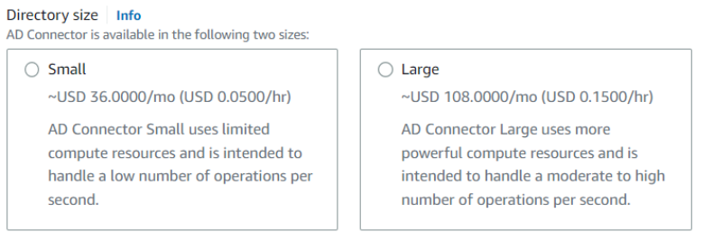
How to Connect Your On-Premises Active Directory to AWS Using AD Connector

Post Syndicated from Jeremy Cowan original https://aws.amazon.com/blogs/security/how-to-connect-your-on-premises-active-directory-to-aws-using-ad-connector/

August 17, 2023: We updated the instructions and screenshots in this post to align with changes to the AWS Management Console.

April 25, 2023: We’ve updated this blog post to include more security learning resources.


AD Connector is designed to give you an easy way to establish a trusted relationship between your Active Directory and AWS. When AD Connector is configured, the trust allows you to:

  • Sign in to AWS applications such as Amazon WorkSpaces, Amazon WorkDocs, and Amazon WorkMail by using your Active Directory credentials.
  • Seamlessly join Windows instances to your Active Directory domain either through the Amazon EC2 launch wizard or programmatically through the EC2 Simple System Manager (SSM) API.
  • Provide federated sign-in to the AWS Management Console by mapping Active Directory identities to AWS Identity and Access Management (IAM) roles.

AD Connector cannot be used with your custom applications, as it is only used for secure AWS integration for the three use-cases mentioned above. Custom applications relying on your on-premises Active Directory should communicate with your domain controllers directly or utilize AWS Managed Microsoft AD rather than integrating with AD Connector. To learn more about which AWS Directory Service solution works best for your organization, see the service documentation.

With AD Connector, you can streamline identity management by extending your user identities from Active Directory. It also enables you to reuse your existing Active Directory security policies such as password expiration, password history, and account lockout policies. Also, your users will no longer need to remember yet another user name and password combination. Since AD Connector doesn’t rely on complex directory synchronization technologies or Active Directory Federation Services (AD FS), you can forego the added cost and complexity of hosting a SAML-based federation infrastructure. In sum, AD Connector helps foster a hybrid environment by allowing you to leverage your existing on-premises investments to control different facets of AWS.

This blog post will show you how AD Connector works as well as walk through how to enable federated console access, assign users to roles, and seamlessly join an EC2 instance to an Active Directory domain.

AD Connector – Under the Hood

AD Connector is a dual Availability Zone proxy service that connects AWS apps to your on-premises directory. AD Connector forwards sign-in requests to your Active Directory domain controllers for authentication and provides the ability for applications to query the directory for data. When you configure AD Connector, you provide it with service account credentials that are securely stored by AWS. This account is used by AWS to enable seamless domain join, single sign-on (SSO), and AWS Applications (WorkSpaces, WorkDocs, and WorkMail) functionality. Given AD Connector’s role as a proxy, it does not store or cache user credentials. Rather, authentication, lookup, and management requests are handled by your Active Directory.

In order to create an AD Connector, you must also provide a pair of DNS IP addresses during setup. These are used by AD Connector to retrieve Service (SRV) DNS records to locate the nearest domain controllers to route requests to. The AD connector proxy instances use an algorithm similar to the Active Directory domain controller locator process to decide which domain controllers to connect to for LDAP and Kerberos requests.

For authentication to AWS applications and the AWS Management Console, you can configure an access URL from the AWS Directory Service console. This access URL is in the format of https://<alias>.awsapps.com and provides a publicly accessible sign-in page. You can visit https://<alias>.awsapps.com/workdocs to sign in to WorkDocs, and https://<alias>.awsapps.com/console to sign in to the AWS Management Console. The following image shows the sign-in page for the AWS Management Console.

Figure 1: Login

Figure 1: Login

For added security you can enable multi-factor authentication (MFA) for AD Connector, but you’ll need to have an existing RADIUS infrastructure in your on-premises network set up to leverage this feature. See AD Connector – Multi-factor Authentication Prerequisites for more information about requirements and configuration. With MFA enabled with AD Connector, the sign-in page hosted at your access URL will prompt users for an MFA code in addition to their standard sign-in credentials.

AD Connector comes in two sizes: small and large. A large AD Connector runs on more powerful compute resources and is more expensive than a small AD Connector. Depending on the volume of traffic to be proxied by AD Connector, you’ll want to select the appropriate size for your needs.

Figure 2: Directory size

Figure 2: Directory size

AD Connector is highly available, meaning underlying hosts are deployed across multiple Availability Zones in the region you deploy. In the event of host-level failure, Directory Service will promptly replace failed hosts. Directory Service also applies performance and security updates automatically to AD Connector.

The following diagram illustrates the authentication flow and network path when you enable AWS Management Console access:

  1. A user opens the secure custom sign-in page and supplies their Active Directory user name and password.
  2. The authentication request is sent over SSL to AD Connector.
  3. AD Connector performs LDAP authentication to Active Directory.

    Note: AD Connector locates the nearest domain controllers by querying the SRV DNS records for the domain.

  4. After the user has been authenticated, AD Connector calls the STS AssumeRole method to get temporary security credentials for that user. Using those temporary security credentials, AD Connector constructs a sign-in URL that users use to access the console.

    Note: If a user is mapped to multiple roles, the user will be presented with a choice at sign-in as to which role they want to assume. The user session is valid for 1 hour.

    Figure 3: Authentication flow and network path

    Figure 3: Authentication flow and network path

Before getting started with configuring AD Connector for federated AWS Management Console access, be sure you’ve read and understand the prerequisites for AD Connector. For example, as shown in Figure 3 there must be a VPN or Direct Connect circuit in place between your VPC and your on-premises environment. Your domain also has to be running at Windows 2003 functional level or later. Also, various ports have to be opened between your VPC and your on-premises environment to allow AD Connector to communicate with your on-premises directory.

Configuring AD Connector for federated AWS Management Console access

Enable console access

To allow users to sign in with their Active Directory credentials, you need to explicitly enable console access. You can do this by opening the Directory Service console and clicking the Directory ID name (Figure 4).

This opens the Directory Details page, where you’ll find a dropdown menu on the Apps & Services tab to enable the directory for AWS Management Console access.

Figure 4: Directories

Figure 4: Directories

Choose the Application management tab as seen in Figure 5.

Figure 5: Application Management

Figure 5: Application Management

Scroll down to AWS Management Console as shown in Figure 6, and choose Enable from the Actions dropdown list.

Figure 6: Enable console access

Figure 6: Enable console access

After enabling console access, you’re ready to start configuring roles and associating Active Directory users and groups with those roles.

Follow these steps to create a new role. When you create a new role through the Directory Service console, AD Connector automatically adds a trust relationship to Directory Service. The following code example shows the IAM trust policy for the role, after a role is created.

{
   "Version": "2012-10-17",
   "Statement": [
     {
       "Sid": "",
       "Effect": "Allow",
       "Principal": {
         "Service": "ds.amazonaws.com"
       },
       "Action": "sts:AssumeRole",
       "Condition": {
         "StringEquals": {
           "sts:externalid": "482242153642"
	  }
	}
     }
   ]
}

Assign users to roles

Now that AD Connector is configured and you’ve created a role, your next job is to assign users or groups to those IAM roles. Role mapping is what governs what resources a user has access to within AWS. To do this you’ll need to do the following steps:

  1. Open the Directory Service console and navigate to the AWS Management Console section.
  2. In the search bar, type the name of the role you just created.
  3. Select the role that you just created by choosing the name under the IAM role field.
  4. Choose Add, and enter the name to be added to find users or groups for this role.
  5. Choose Add, and the user or group is now assigned to the role.

When you’re finished, you should see the name of the user or group along with the corresponding ID for that object. It is also important to note that this list can be used to remove users or groups from the role. The next time the user signs in to the AWS Management Console from the custom sign-in page, they will be signed in under the EC2ReadOnly security role.

Seamlessly join an instance to an Active Directory domain

Another advantage to using AD Connector is the ability to seamlessly join Windows (EC2) instances to your Active Directory domain. This allows you to join a Windows Server to the domain while the instance is being provisioned instead of using a script or doing it manually. This section of this blog post will explain the steps necessary to enable this feature in your environment and how the service works.

Step 1: Create a role

Until recently you had to manually create an IAM policy to allow an EC2 instance to access the SSM, an AWS service that allows you to configure Windows instances while they’re running and on first launch. Now, there’s a managed policy called AmazonEC2RoleforSSM that you can use instead. The role you are about to create will be assigned to an EC2 instance when it’s provisioned, which will grant it permission to access the SSM service.

To create the role:

  1. Open the IAM console.
  2. Click Roles in the navigation pane.
  3. Click Create Role.
  4. Type a name for your role in the Role Name field.
  5. Under AWS Service Roles, select Amazon EC2 and then click Select.
  6. On the Attach Policy page, select AmazonEC2RoleforSSM and then click Next Step.
  7. On the Review page, click Create Role.

If you click the role you created, you’ll see a trust policy for EC2, which looks like the following code example.

{
     "Version": "2012-10-17",
     "Statement": [
       {
         "Sid": "",
         "Effect": "Allow",
         "Principal": {
           "Service": "ec2.amazonaws.com"
         },
         "Action": "sts:AssumeRole"
       }
     ]
}

Step 2: Create a new Windows instance from the EC2 console

With this role in place, you can now join a Windows instance to your domain via the EC2 launch wizard. For a detailed explanation about how to do this, see Joining a Domain Using the Amazon EC2 Launch Wizard.

If you’re instantiating a new instance from the API, however, you will need to create an SSM configuration document and upload it to the SSM service beforehand. We’ll step through that process next.

Note: The instance will require internet access to communicate with the SSM service.

Figure 7: Configure instance details

Figure 7: Configure instance details

When you create a new Windows instance from the EC2 launch wizard as shown in Figure 7, the wizard automatically creates the SSM configuration document from the information stored in AD Connector. Presently, the EC2 launch wizard doesn’t allow you to specify which organizational unit (OU) you want to deploy the member server into.

Step 3: Create an SSM document (for seamlessly joining a server to the domain through the AWS API)

If you want to provision new Windows instances from the AWS CLI or API or you want to specify the target OU for your instances, you will need to create an SSM configuration document. The configuration document is a JSON file that contains various parameters used to configure your instances. The following code example is a configuration document for joining a domain.

{
	"schemaVersion": "1.0",
	"description": "Sample configuration to join an instance to a domain",
	"runtimeConfig": {
	   "aws:domainJoin": {
	       "properties": {
	          "directoryId": "d-1234567890",
	          "directoryName": "test.example.com",
	          "directoryOU": "OU=test,DC=example,DC=com",
	          "dnsIpAddresses": [
	             "198.51.100.1",
	             "198.51.100.2"
	          ]
	       }
	   }
	}
}

In this configuration document:

  • directoryId is the ID for the AD Connector you created earlier.
  • directoryName is the name of the domain (for example, examplecompany.com).
  • directoryOU is the OU for the domain.
  • dnsIpAddresses are the IP addresses for the DNS servers you specified when you created the AD Connector.

For additional information, see aws:domainJoin. When you’re finished creating the file, save it as a JSON file.

Note: The name of the file has to be at least 1 character and at most 64 characters in length.

Step 4: Upload the configuration document to SSM

This step requires that the user have permission to use SSM to configure an instance. If you don’t have a policy that includes these rights, create a new policy by using the following JSON, and assign it to an IAM user or group.

{
   "Version": "2012-10-17",
   "Statement": [
     {
       "Effect": "Allow",
       "Action": "ssm:*",
       "Resource": "*"
     }
   ]
}

After you’ve signed in with a user that associates with the SSM IAM policy you created, run the following command from the AWS CLI.

aws ssm create-document ‐‐content file://path/to/myconfigfile.json ‐‐name "My_Custom_Config_File"

Note: On Linux/Mac systems, you need to add a “/” at the beginning of the path (for example, file:///Users/username/temp).

This command uploads the configuration document you created to the SSM service, allowing you to reference it when creating a new Windows instance from either the AWS CLI or the EC2 launch wizard.

Conclusion

This blog post has shown you how you can simplify account management by federating with your Active Directory for AWS Management Console access. The post also explored how you can enable hybrid IT by using AD Connector to seamlessly join Windows instances to your Active Directory domain. Armed with this information you can create a trust between your Active Directory and AWS. In addition, you now have a quick and simple way to enable single sign-on without needing to replicate identities or deploy additional infrastructure on premises.

We’d love to hear more about how you are using Directory Service, and welcome any feedback about how we can improve the experience. You can post comments below, or visit the Directory Service forum to post comments and questions.

If you have feedback about this post, submit comments in the Comments section below. If you have questions about this post, start a new thread on the AWS Directory Service knowledge Center re:Post or contact AWS Support.

Want more AWS Security news? Follow us on Twitter.

Jeremy Cowan

Jeremy Cowan

Jeremy is a Specialist Solutions Architect for containers at AWS, although his family thinks he sells “cloud space”. Prior to joining AWS, Jeremy worked for several large software vendors, including VMware, Microsoft, and IBM. When he’s not working, you can usually find on a trail in the wilderness, far away from technology.

Bright Dike

Bright Dike

Bright is a Solutions Architect with Amazon Web Services. He works with AWS customers and partners to provide guidance assessing and improving their security posture, as well as executing automated remediation techniques. His domains are threat detection, incident response, and security hub.

David Selberg

David Selberg

David is an Enterprise Solutions Architect at AWS who is passionate about helping customers build Well-Architected solutions on the AWS cloud. With a background in cybersecurity, David loves to dive deep on security topics when he’s not creating technical content like the “All Things AWS” Twitch series.

Abhra Sinha

Abhra Sinha

Abhra is a Toronto-based Enterprise Solutions Architect at AWS. Abhra enjoys being a trusted advisor to customers, working closely with them to solve their technical challenges and help build a secure scalable architecture on AWS. In his spare time, he enjoys photography and exploring new restaurants.

How to automate the review and validation of permissions for users and groups in AWS IAM Identity Center

Post Syndicated from Yee Fei Ooi original https://aws.amazon.com/blogs/security/how-to-automate-the-review-and-validation-of-permissions-for-users-and-groups-in-aws-iam-identity-center/

AWS IAM Identity Center (successor to AWS Single Sign-On) is widely used by organizations to centrally manage federated access to their Amazon Web Services (AWS) environment. As organizations grow, it’s crucial that they maintain control of access to their environment and conduct regular reviews of existing granted permissions to maintain a good security posture. With continuous movement of users among projects and teams within an organization, there are constant updates in groups and permission sets. Given the frequency of updates, it’s important for organizations to maintain the integrity of the identity entities and promote visibility into their associated permissions within IAM Identity Center.

Performing an audit of permissions assignment through the IAM Identity Center Management Console can be an arduous and time-consuming task, especially for customers managing a significant number of AWS accounts. This blog post addresses the following concerns faced by security administrators:

  • How to maintain control over permissions and efficiently conduct thorough audits.
  • How to regularly review granted permissions to uphold the principle of least privilege.

In this blog post, we show you how to automate your IAM Identity Center users and groups permission review process with AWS SDK and AWS serverless services. The solution also includes how to schedule the review process based on preferred frequency and generating a business-specific access and permission review report.

By using AWS serverless services and AWS SDK, you can create an automated workflow to retrieve the latest permission sets of your identities in IAM Identity Center and extract them as a report. Amazon EventBridge scheduling allows you to set customized schedules to launch the automation process. AWS Lambda functions are used in data retrieval, data transformation, and report generation, and Amazon DynamoDB tables are used for storing raw unstructured data.

We show you how to build an automated solution using AWS SDK, AWS Step Functions, Lambda, DynamoDB, EventBridge, Amazon Simple Storage Service (Amazon S3), and Amazon Simple Notification Service (Amazon SNS) to review the IAM Identity Center instance that you specify. The review includes retrieving attached permission policies (inline, AWS managed, and customer managed) based on the assigned identity.

Note: This solution will incur costs based on the AWS services used.

Prerequisites

In your own AWS environment, make sure that you have the following:

  • An IAM Identity Center instance set up in the account
  • IAM Identity Center instance metadata that you want to perform the analysis on:
    • The IAM Identity Center instance identityStoreId – example: d-xxxxxxxxxx
    • The IAM Identity Center instance instanceArn – example: arn:aws:sso:::instance/ssoins-xxxxxxxxxx
  • Access and permission to deploy the related AWS services mentioned previously in AWS CloudFormation.

    Note: This solution is expected to deploy in the account where your IAM Identity Center instance is being set up. If you want to deploy in other accounts, you need to establish cross-account access for the IAM roles of the relevant services mentioned previously.

  • AWS SAM CLI installed. You will deploy the solution using AWS Serverless Application Model (AWS SAM). To learn more about how AWS SAM works, see the AWS Serverless Application Model (AWS SAM) specification.

Solution overview

In this section, we discuss the steps to set up solution. We provide a CloudFormation template that you can use to set up the required services and Lambda functions. Figure 1 illustrates the architecture of the solution.

Figure 1: Architecture of the solution

Figure 1: Architecture of the solution

The solution is deployed using AWS SAM, which is an open-sourced framework for building serverless applications. AWS SAM helps to organize related components and operate on a single stack. When used together with the SAM CLI, it’s a useful tool for developing, testing, and building serverless applications on AWS.

To generate the report, the solution uses the following steps:

  • The EventBridge Scheduler is configured to launch the Step Functions based on the frequency of the cron job stated. The user can also manually launch the review as needed.
  • After the Step Functions are launched, the dataExtractionFunction Lambda function retrieves data from IAM Identity Center and stores it in two separate DynamoDB tables, fullPermissionSetsWithGroupTable and userWithGroupTable.
  • Step Functions will then launch the dataTransformLoadFunction Lambda function, which retrieves the data from both DynamoDB tables to perform data transformation for report generation.
  • The permission review report is stored in an S3 bucket and notification of completion is sent to the stakeholders.

Deploy the solution

  1. Make sure that you have AWS SAM CLI installed.
  2. Clone the GitHub repository. Open a CLI window and run
    git clone https://github.com/aws-samples/aws-iam-identity-center-permission-policies-analyzer.git
  3. Navigate to root directory of the GitHub repository by running cd aws-iam-identity-center-permission-policies-analyzer
  4. Run sam deploy ‐‐guided and follow the step-by-step instructions to indicate the deployment details such as the desired CloudFormation stack name, AWS Region and other details as shown in Figure 2.
     
    Figure 2: Configure SAM deploy

    Figure 2: Configure SAM deploy

  5. As shown in Figure 2, you receive confirmation that the required resources have been created. AWS SAM creates a default S3 bucket to store the necessary resources and then proceeds to the deployment prompt. Enter y to deploy and wait for deployment to complete.
  6. After deployment is complete, you should see the following output: Successfully created/updated stack – {StackName} in {AWSRegion}. You can review the resources and stack in your CloudFormation console as shown in Figure 3.
     
    Figure 3: CloudFormation console view of deployed stack

    Figure 3: CloudFormation console view of deployed stack

    The CloudFormation template specifies the cron schedule on the first day of each month at 0800 UTC +8 by default. You can update the schedule based on your preference by following steps 7 and 8.

  7. Open the EventBridge console. In the navigation pane, under Scheduler, choose Schedules. Check the box next to {StackName}-monthlySchedule-{RandomID} and choose Edit.
     
    Figure 4: EventBridge schedule console

    Figure 4: EventBridge schedule console

  8. At Step 1, under the Schedule pattern segment, enter your preferred scheduling. To learn about the different types of EventBridge scheduling, see Schedule types on EventBridge Scheduler. For this example, you use a recurring type of schedule using cron expression. Update to your preferred schedule and time zone and choose Next.
     
    Figure 5: EventBridge Schedule edit console Step 1 – Specify schedule detail

    Figure 5: EventBridge Schedule edit console Step 1 – Specify schedule detail

  9. Check the email address you entered during the deployment stage of this solution for an email sent by [email protected], similar to what you see in Figure 6. Follow the steps in the email to confirm the Amazon SNS topic subscription.
     
    Figure 6: Example email from Amazon SNS for subscription confirmation

    Figure 6: Example email from Amazon SNS for subscription confirmation

Manually launch the review

After you’ve updated the schedule, the review process runs on the specified timing and frequency. You can manually launch the review immediately after you’ve deployed the solution, or at a time outside of the schedule on an as-needed basis.

  1. To manually launch the review, open the Step Functions console,
  2. Select the state machine monthlyUserPermissionAssessment-{randomID} and choose Start execution.
     
    Figure 7: Start execution for monthlyUserPermissionAssessment state machine

    Figure 7: Start execution for monthlyUserPermissionAssessment state machine

  3. Enter the following event pattern and choose Start execution.
    {
      "identityStoreId": "d-xxxxxxxxxx",
      "instanceArn": "arn:aws:sso:::instance/ssoins-xxxxxxxxxx",
      "ssoDeployedRegion": "YOUR_SSO_DEPLOYED_REGION" 
    }

    Note: The format and keyword format are important to run the Step Functions successfully.

Figure 8: Example input to start state machine execution

Figure 8: Example input to start state machine execution

When the process starts, the execution page opens and you can follow the process. The flow turns green when each step has been completed successfully. You can also review Events and check the Lambda functions or logs if you need to troubleshoot or refer to the details.

Figure 9: State machine successful execution example

Figure 9: State machine successful execution example

Notification from each successful review

After each successful execution, you should receive an email notification at the email you specified in the Amazon SNS topic. You can then retrieve the report from the S3 bucket with the bucket name {StackName}-monthlyre-{AccountID}. Your report is stored according to the object key name specified in the email. An example of the email notification is shown in Figure 10.

Figure 10: Example email notification

Figure 10: Example email notification

You can download the report in CSV format from the S3 bucket. The headers of the report are:

User: Username
PrincipalId: An identifier for an object in IAM Identity Center, such as a user or group
PrincipalType: USER or GROUP
GroupName: Group’s display name value (if PrincipalType is GROUP)
AccountIdAssignment: Identifier of the AWS account assigned with the specified permission set
PermissionSetARN: ARN of the permission set
PermissionSetName: Name of the permission set
Inline Policy: Inline policy that is attached to the permission set
Customer Managed Policy: Specifies the names and paths of the customer managed policies that you have attached to your permission set
AWS Managed Policy: Details of the AWS managed policy
Permission Boundary: Permission boundary details (Customer Managed Policy Reference and/or AWS managed policy ARN)

From the report, you can determine whether a user is assigned to an account individually or as part of a group, along with the corresponding permission sets. The report also includes details on inline policy, AWS managed policy, customer managed policy, and the permission boundaries attached to the permission set. Inline policies and AWS managed policies are presented in JSON format. However, for customer managed policies and permission boundaries, to keep the solution simple, the generated report provides only basic information on the policies that you’ve attached to the permission set. You can log in to the respective accounts to view the policies in full JSON format through the AWS IAM console.

[Optional] Customize the user notification email

If you want to customize the email notification subject and content, you can do so by editing the Lambda function {StackName}-dataTransformLoadFunction-{RandomID}. Scroll down to the bottom of the source code and edit the sns_message and Subject accordingly.

Figure 11: Customizing the notification email in dataTransformLoadFunction source code

Figure 11: Customizing the notification email in dataTransformLoadFunction source code

Clean up the resources

To clean up the resources that you created for this example:

  1. Empty your S3 bucket. Open the Amazon S3 console, search for the bucket name and choose Empty. Follow the instructions on screen to empty it.
  2. Delete the CloudFormation stack by either:
    1. Using the CloudFormation console to delete the stack, or
    2. Using the AWS SAM CLI to run sam delete in your terminal. Follow the instructions and enter y when prompted to delete the stack.

Conclusion

In this post, you learned how to deploy a solution that simplifies the review and analysis of IAM permissions granted to IAM Identity Center with an automated flow. You also learned about customization that you can set up to fit your team’s needs and preferences.

If you have feedback about this post, submit comments in the Comments section. If you have questions about this post, start a new thread on the AWS Security, Identity, & Compliance re:Post or contact AWS Support.

Want more AWS Security news? Follow us on Twitter.

Yee Fei Ooi

Yee Fei Ooi

Yee Fei is a Solutions Architect supporting independent software vendor (ISV) customers in Singapore and is part of the Containers TFC. She enjoys helping her customers to grow their businesses and build solutions that automate, innovate, and improve efficiency.

ZhiWei Huang

Edmund Yeo

Edmund is a Security Solutions Architect who helps customers build confidently and securely on AWS. He shares with customers his expertise in AWS security and advocates to build with security best practices in mind. He brings a combination of perspective and experience to help small and medium businesses in ASEAN to improve their security posture.

ZhiWei Huang

ZhiWei Huang

ZhiWei is a Financial Services Solutions Architect at AWS. He works with FSI customers across the ASEAN region, providing guidance for establishing robust security controls and networking foundations as customers build on and scale with AWS. Outside of work, he finds joy in travelling the world and spending quality time with his family.

Derive operational insights from application logs using Automated Data Analytics on AWS

Post Syndicated from Aparajithan Vaidyanathan original https://aws.amazon.com/blogs/big-data/derive-operational-insights-from-application-logs-using-automated-data-analytics-on-aws/

Automated Data Analytics (ADA) on AWS is an AWS solution that enables you to derive meaningful insights from data in a matter of minutes through a simple and intuitive user interface. ADA offers an AWS-native data analytics platform that is ready to use out of the box by data analysts for a variety of use cases. With ADA, teams can ingest, transform, govern, and query diverse datasets from a range of data sources without requiring specialist technical skills. ADA provides a set of pre-built connectors to ingest data from a wide range of sources including Amazon Simple Storage Service (Amazon S3), Amazon Kinesis Data Streams, Amazon CloudWatch, Amazon CloudTrail, and Amazon DynamoDB as well as many others.

ADA provides a foundational platform that can be used by data analysts in a diverse set of use cases including IT, finance, marketing, sales, and security. ADA’s out-of-the-box CloudWatch data connector allows data ingestion from CloudWatch logs in the same AWS account in which ADA has been deployed, or from a different AWS account.

In this post, we demonstrate how an application developer or application tester is able to use ADA to derive operational insights of applications running in AWS. We also demonstrate how you can use the ADA solution to connect to different data sources in AWS. We first deploy the ADA solution into an AWS account and set up the ADA solution by creating data products using data connectors. We then use the ADA Query Workbench to join the separate datasets and query the correlated data, using familiar Structured Query Language (SQL), to gain insights. We also demonstrate how ADA can be integrated with business intelligence (BI) tools such as Tableau to visualize the data and to build reports.

Solution overview

In this section, we present the solution architecture for the demo and explain the workflow. For the purposes of demonstration, the bespoke application is simulated using an AWS Lambda function that emits logs in Apache Log Format at a preset interval using Amazon EventBridge. This standard format can be produced by many different web servers and be read by many log analysis programs. The application (Lambda function) logs are sent to a CloudWatch log group. The historical application logs are stored in an S3 bucket for reference and for querying purposes. A lookup table with a list of HTTP status codes along with the descriptions is stored in a DynamoDB table. These three serve as sources from which data is ingested into ADA for correlation, query, and analysis. We deploy the ADA solution into an AWS account and set up ADA. We then create the data products within ADA for the CloudWatch log group, S3 bucket, and DynamoDB. As the data products are configured, ADA provisions data pipelines to ingest the data from the sources. With the ADA Query Workbench, you can query the ingested data using plain SQL for application troubleshooting or issue diagnosis.

The following diagram provides an overview of the architecture and workflow of using ADA to gain insights into application logs.

The workflow includes the following steps:

  1. A Lambda function is scheduled to be triggered at 2-minute intervals using EventBridge.
  2. The Lambda function emits logs that are stored at a specified CloudWatch log group under /aws/lambda/CdkStack-AdaLogGenLambdaFunction. The application logs are generated using the Apache Log Format schema but stored in the CloudWatch log group in JSON format.
  3. The data products for CloudWatch, Amazon S3, and DynamoDB are created in ADA. The CloudWatch data product connects to the CloudWatch log group where the application (Lambda function) logs are stored. The Amazon S3 connector connects to an S3 bucket folder where the historical logs are stored. The DynamoDB connector connects to a DynamoDB table where the status codes that are referred by the application and historical logs are stored.
  4. For each of the data products, ADA deploys the data pipeline infrastructure to ingest data from the sources. When the data ingestion is complete, you can write queries using SQL via the ADA Query Workbench.
  5. You can log in to the ADA portal and compose SQL queries from the Query Workbench to gain insights in to the application logs. You can optionally save the query and share the query with other ADA users in the same domain. The ADA query feature is powered by Amazon Athena, which is a serverless, interactive analytics service that provides a simplified, flexible way to analyze petabytes of data.
  6. Tableau is configured to access the ADA data products via ADA egress endpoints. You then create a dashboard with two charts. The first chart is a heat map that shows the prevalence of HTTP error codes correlated with the application API endpoints. The second chart is a bar chart that shows the top 10 application APIs with a total count of HTTP error codes from the historical data.

Prerequisites

For this post, you need to complete the following prerequisites:

  1. Install the AWS Command Line Interface (AWS CLI), AWS Cloud Development Kit (AWS CDK) prerequisites, TypeScript-specific prerequisites, and git.
  2. Deploy the ADA solution in your AWS account in the us-east-1 Region.
    1. Provide an admin email while launching the ADA AWS CloudFormation stack. This is needed for ADA to send the root user password. An admin phone number is required to receive a one-time password message if multi-factor authentication (MFA) is enabled. For this demo, MFA is not enabled.
  3. Build and deploy the sample application (available on the GitHub repo) solution so that the following resources can be provisioned in your account in the us-east-1 Region:
    1. A Lambda function that simulates the logging application and an EventBridge rule that invokes the application function at 2-minute intervals.
    2. An S3 bucket with the relevant bucket policies and a CSV file that contains the historical application logs.
    3. A DynamoDB table with the lookup data.
    4. Relevant AWS Identity and Access Management (IAM) roles and permissions required for the services.
  4. Optionally, install Tableau Desktop, a third-party BI provider. For this post, we use Tableau Desktop version 2021.2. There is a cost involved in using a licensed version of the Tableau Desktop application. For additional details, refer to the Tableau licensing information.

Deploy and set up ADA

After ADA is deployed successfully, you can log in using the admin email provided during the installation. You then create a domain named CW_Domain. A domain is a user-defined collection of data products. For example, a domain might be a team or a project. Domains provide a structured way for users to organize their data products and manage access permissions.

  1. On the ADA console, choose Domains in the navigation pane.
  2. Choose Create domain.
  3. Enter a name (CW_Domain) and description, then choose Submit.

Set up the sample application infrastructure using AWS CDK

The AWS CDK solution that deploys the demo application is hosted on GitHub. The steps to clone the repo and to set up the AWS CDK project are detailed in this section. Before you run these commands, be sure to configure your AWS credentials. Create a folder, open the terminal, and navigate to the folder where the AWS CDK solution needs to be installed. Run the following code:

gh repo clone aws-samples/operational-insights-with-automated-data-analytics-on-aws
cd operational-insights-with-automated-data-analytics-on-aws
npm install
npm run build
cdk synth
cdk deploy

These steps perform the following actions:

  • Install the library dependencies
  • Build the project
  • Generate a valid CloudFormation template
  • Deploy the stack using AWS CloudFormation in your AWS account

The deployment takes about 1–2 minutes and creates the DynamoDB lookup table, Lambda function, and S3 bucket containing the historical log files as outputs. Copy these values to a text editing application, such as Notepad.

Create ADA data products

We create three different data products for this demo, one for each data source that you’ll be querying to gain operational insights. A data product is a dataset (a collection of data such as a table or a CSV file) that has been successfully imported into ADA and that can be queried.

Create a CloudWatch data product

First, we create a data product for the application logs by setting up ADA to ingest the CloudWatch log group for the sample application (Lambda function). Use the CdkStack.LambdaFunction output to get the Lambda function ARN and locate the corresponding CloudWatch log group ARN on the CloudWatch console.

Then complete the following steps:

  1. On the ADA console, navigate to the ADA domain and create a CloudWatch data product.
  2. For Name¸ enter a name.
  3. For Source type, choose Amazon CloudWatch.
  4. Disable Automatic PII.

ADA has a feature that automatically detects personally identifiable information (PII) data during import that is enabled by default. For this demo, we disable this option for the data product because the discovery of PII data is not in the scope of this demo.

  1. Choose Next.
  2. Search for and choose the CloudWatch log group ARN copied from the previous step.
  3. Copy the log group ARN.
  4. On the data product page, enter the log group ARN.
  5. For CloudWatch Query, enter a query that you want ADA to get from the log group.

In this demo, we query the @message field because we’re interested in getting the application logs from the log group.

  1. Select how the data updates are triggered after initial import.

ADA can be configured to ingest the data from the source at flexible intervals (up to 15 minutes or later) or on demand. For the demo, we set the data updates to run hourly.

  1. Choose Next.

Next, ADA will connect to the log group and query the schema. Because the logs are in Apache Log Format, we transform the logs into separate fields so that we can run queries on the specific log fields. ADA provides four default transformations and supports custom transformation through a Python script. In this demo, we run a custom Python script to transform the JSON message field into Apache Log Format fields.

  1. Choose Transform schema.
  2. Choose Create new transform.
  3. Upload the apache-log-extractor-transform.py script from the /asset/transform_logs/ folder.
  4. Choose Submit.

ADA will transform the CloudWatch logs using the script and present the processed schema.

  1. Choose Next.
  2. In the last step, review the steps and choose Submit.

ADA will start the data processing, create the data pipelines, and prepare the CloudWatch log groups to be queried from the Query Workbench. This process will take a few minutes to complete and will be shown on the ADA console under Data Products.

Create an Amazon S3 data product

We repeat the steps to add the historical logs from the Amazon S3 data source and look up reference data from the DynamoDB table. For these two data sources, we don’t create custom transforms because the data formats are in CSV (for historical logs) and key attributes (for reference lookup data).

  1. On the ADA console, create a new data product.
  2. Enter a name (hist_logs) and choose Amazon S3.
  3. Copy the Amazon S3 URI (the text after arn:aws:s3:::) from the CdkStack.S3 output variable and navigate to the Amazon S3 console.
  4. In the search box, enter the copied text, open the S3 bucket, select the /logs folder, and choose Copy S3 URI.

The historical logs are stored in this path.

  1. Navigate back to the ADA console and enter the copied S3 URI for S3 location.
  2. For Update Trigger, select On Demand because the historical logs are updated at an unspecified frequency.
  3. For Update Policy, select Append to append newly imported data to the existing data.
  4. Choose Next.

ADA processes the schema for the files in the selected folder path. Because the logs are in CSV format, ADA is able to read the column names without requiring additional transformations. However, the columns status_code and request_size are inferred as long type by ADA. We want to keep the column data types consistent among the data products so that we can join the data tables and query the data. The column status_code will be used to create joins across the data tables.

  1. Choose Transform schema to change the data types of the two columns to string data type.

Note the highlighted column names in the Schema preview pane prior to applying the data type transformations.

  1. In the Transform plan pane, under Built-in transforms, choose Apply Mapping.

This option allows you to change the data type from one type to another.

  1. In the Apply Mapping section, deselect Drop other fields.

If this option is not disabled, only the transformed columns will be preserved and all other columns will be dropped. Because we want to retain all the columns, we disable this option.

  1. Under Field Mappings¸ for Old name and New name, enter status_code and for New type, enter string.
  2. Choose Add Item.
  3. For Old name and New name¸ enter request_size and for New data type, enter string.
  4. Choose Submit.

ADA will apply the mapping transformation on the Amazon S3 data source. Note the column types in the Schema preview pane.

  1. Choose View sample to preview the data with the transformation applied.

ADA will display the PII data acknowledgement to ensure that either only authorized users can view the data or that the dataset doesn’t contain any PII data.

  1. Choose Agree to continue to view the sample data.

Note that the schema is identical to the CloudWatch log group schema because both the current application and historical application logs are in Apache Log Format.

  1. In the final step, review the configuration and choose Submit.

ADA starts processing the data from the Amazon S3 source, creates the backend infrastructure, and prepares the data product. This process takes a few minutes depending upon the size of the data.

Create a DynamoDB data product

Lastly, we create a DynamoDB data product. Complete the following steps:

  1. On the ADA console, create a new data product.
  2. Enter a name (lookup) and choose Amazon DynamoDB.
  3. Enter the Cdk.DynamoDBTable output variable for DynamoDB Table ARN.

This table contains key attributes that will be used as a lookup table in this demo. For the lookup data, we are using the HTTP codes and long and short descriptions of the codes. You can also use PostgreSQL, MySQL, or a CSV file source as an alternative.

  1. For Update Trigger, select On-Demand.

The updates will be on demand because the lookup is mostly for reference purpose while querying and any updates to the lookup data can be updated in ADA using on-demand triggers.

  1. Choose Next.

ADA reads the schema from the underlying DynamoDB schema and presents the column name and type for optional transformation. We will proceed with the default schema selection because the column types are consistent with the types from the CloudWatch log group and Amazon S3 CSV data source. Having data types that are consistent across the data sources allows us to write queries to fetch records by joining the tables using the column fields. For example, the column key in the DynamoDB schema corresponds to the status_code in the Amazon S3 and CloudWatch data products. We can write queries that can join the three tables using the column name key. An example is shown in the next section.

  1. Choose Continue with current schema.
  2. Review the configuration and choose Submit.

ADA will process the data from the DynamoDB table data source and prepare the data product. Depending upon the size of the data, this process takes a few minutes.

Now we have all the three data products processed by ADA and available for you to run queries.

Use the Query Workbench to query the data

ADA allows you to run queries against the data products while abstracting the data source and making it accessible using SQL (Structured Query Language). You can write queries and join the tables just as you would query against tables in a relational database. We demonstrate ADA’s querying capability via two user scenarios. In both the scenarios, we join an application log dataset to the error codes lookup table. In the first use case, we query the current application logs to identify the top 10 most accessed application endpoints along with the corresponding HTTP status codes:

--Query the top 10 Application endpoints along with the corresponding HTTP request type and HTTP status code.

SELECT logs.endpoint AS Application_EndPoint, logs.http_request AS REQUEST, count(logs.endpoint) as Endpoint_Count, ref.key as HTTP_Status_Code, ref.short as Description
FROM cw_domain.cloud_watch_application_logs logs
INNER JOIN cw_domain.lookup ref ON logs.status_code = ref.key
where logs.status_code LIKE '4%%' OR logs.status_code LIKE '5%%' -- = '/v1/server'
GROUP BY logs.endpoint, logs.http_request, ref.key, ref.short
ORDER BY Endpoint_Count DESC
LIMIT 10

In the second example, we query the historical logs table to get the top 10 application endpoints with the most errors to understand the endpoint call pattern:

-- Query Historical Logs to get the top 10 Application Endpoints with most number of errors along with an explanation of the error code.

SELECT endpoint as Application_EndPoint, count(status_code) as Error_Count, ref.long as Description FROM cw_domain.hist_logs hist
INNER JOIN cw_domain.lookup ref ON hist.status_code = ref.key
WHERE hist.status_code LIKE '4%%' OR hist.status_code LIKE '5%%'
GROUP BY endpoint, status_code, ref.long
ORDER BY Error_Count desc
LIMIT 10

In addition to querying, you can optionally save the query and share the saved query with other users in the same domain. The shared queries are accessible directly from the Query Workbench. The query results can also be exported to CSV format.

Visualize ADA data products in Tableau

ADA offers the ability to connect to third-party BI tools to visualize data and create reports from the ADA data products. In this demo, we use ADA’s native integration with Tableau to visualize the data from the three data products we configured earlier. Using Tableau’s Athena connector and following the steps in Tableau configuration, you can configure ADA as a data source in Tableau. After a successful connection has been established between Tableau and ADA, Tableau will populate the three data products under the Tableau catalog cw_domain.

We then establish a relationship across the three databases using the HTTP status code as the joining column, as shown in the following screenshot. Tableau allows us to work in online and offline mode with the data sources. In online mode, Tableau will connect to ADA and query the data products live. In offline mode, we can use the Extract option to extract the data from ADA and import the data in to Tableau. In this demo, we import the data in to Tableau to make the querying more responsive. We then save the Tableau workbook. We can inspect the data from the data sources by choosing the database and Update Now.

With the data source configurations in place in Tableau, we can create custom reports, charts, and visualizations on the ADA data products. Let’s consider two use cases for visualizations.

As shown in the following figure, we visualized the frequency of the HTTP errors by application endpoints using Tableau’s built-in heat map chart. We filtered out the HTTP status codes to only include error codes in the 4xx and 5xx range.

We also created a bar chart to depict the application endpoints from the historical logs ordered by the count of HTTP error codes. In this chart, we can see that the /v1/server/admin endpoint has generated the most HTTP error status codes.

Clean up

Cleaning up the sample application infrastructure is a two-step process. First, to remove the infrastructure provisioned for the purposes of this demo, run the following command in the terminal:

cdk destroy

For the following question, enter y and AWS CDK will delete the resources deployed for the demo:

Are you sure you want to delete: CdkStack (y/n)? y

Alternatively, you can remove the resources via the AWS CloudFormation console by navigating to the CdkStack stack and choosing Delete.

The second step is to uninstall ADA. For instructions, refer to Uninstall the solution.

Conclusion

In this post, we demonstrated how to use the ADA solution to derive insights from application logs stored across two different data sources. We demonstrated how to install ADA on an AWS account and deploy the demo components using AWS CDK. We created data products in ADA and configured the data products with the respective data sources using the ADA’s built-in data connectors. We demonstrated how to query the data products using standard SQL queries and generate insights on the log data. We also connected the Tableau Desktop client, a third-party BI product, to ADA and demonstrated how to build visualizations against the data products.

ADA automates the process of ingesting, transforming, governing, and querying diverse datasets and simplifying the lifecycle management of data. ADA’s pre-built connectors allow you to ingest data from diverse data sources. Software teams with basic knowledge of AWS products and services will be able to set up an operational data analytics platform in a few hours and provide secure access to the data. The data can then be easily and quickly queried using an intuitive and standalone web user interface.

Try out ADA today to easily manage and gain insights from data.


About the authors

Aparajithan Vaidyanathan is a Principal Enterprise Solutions Architect at AWS. He supports enterprise customers migrate and modernize their workloads on AWS cloud. He is a Cloud Architect with 23+ years of experience designing and developing enterprise, large-scale and distributed software systems. He specializes in Machine Learning & Data Analytics with focus on Data and Feature Engineering domain. He is an aspiring marathon runner and his hobbies include hiking, bike riding and spending time with his wife and two boys.

Rashim Rahman is a Software Developer based out of Sydney, Australia with 10+ years of experience in software development and architecture. He works primarily on building large scale open-source AWS solutions for common customer use cases and business problems. In his spare time, he enjoys sports and spending time with friends and family.

Hafiz Saadullah is a Principal Technical Product Manager at Amazon Web Services. Hafiz focuses on AWS Solutions, designed to help customers by addressing common business problems and use cases.