Post Syndicated from Julian Wood original https://aws.amazon.com/blogs/compute/serverless-icymi-q2-2024/
Welcome to the 26th edition of the AWS Serverless ICYMI (in case you missed it) quarterly recap. Every quarter, we share all the most recent product launches, feature enhancements, blog posts, webinars, live streams, and other interesting things that you might have missed!
In case you missed our last ICYMI, check out what happened last quarter here.

Calendar
EDA Day – London 2024
The AWS Serverless DA team hosted the third Event-Driven Architecture (EDA) Day in London on May 14th. This event brought together prominent figures in the event-driven architecture community, AWS, and customer speakers.
EDA Day covered 13 sessions, 2 workshops, and a Q&A panel. David Boyne was the keynote speaker with a talk “Complexity is the Gotcha of Event-Driven Architecture”. There were AWS speakers including Matthew Meckes, Natasha Wright, Julian Wood, Gillian Amstrong, Josh Kahn, Veda Ramen, and Uma Ramadoss. There was also an impressive lineup of guest speakers, Daniele Frasca, David Anderson, Ryan Cormack, Sarah Hamilton, Sheen Brisals, Marcin Sodkiewicz, and Ben Ellerby.
Videos are available on YouTube

EDA Day London
The future of Serverless
There has been a lot of talk about the future of serverless, with this year being the 10th anniversary of AWS Lambda. Eric Johnson addresses the topic in his ServerlessDays Milan keynote, “Now serverless is all grown up, what’s next”.
AWS Lambda
AWS launched support for the latest release of Ruby 3.3 is based on the new Amazon Linux 2023 runtime. The Ruby 3.3 runtime also provides access to the latest Ruby language features.
There is a new guide on how to retrieve data about Lambda functions that use a deprecated runtime.
Learn how to run code after returning a response from an AWS Lambda function. This post shows how to return a synchronous function response as soon as possible, yet also perform additional asynchronous work after you send the response. For example, you may store data in a database or send information to a logging system.
See how you can use the circuit-breaker pattern with Lambda extensions and Amazon DynamoDB. The circuit breaker pattern can help prevent cascading failures and improve overall system stability.

Circuit-breaker pattern
Lambda functions now scale up to 12X faster in the AWS GovCloud (US) Regions.
Powertools for AWS Lambda (Python) adds support for Agents for Amazon Bedrock.
The AWS SDK for JavaScript v2 enters maintenance mode on September 8, 2024 and reaches end-of-support on September 8, 2025.
Amazon CloudWatch Logs introduced Live Tail streaming CLI support.
Amazon ECS and AWS Fargate
You can now secure Amazon Elastic Container Service (Amazon ECS) workloads on AWS Fargate with customer managed keys (CMKs). Once you add your keys to AWS Key Management Service (AWS KMS), you can use these to encrypt the underlying ephemeral storage of an Amazon ECS task on AWS Fargate.
Windows containers on AWS Fargate now start faster, up to 42% for Windows Server 2022 Core. AWS has optimized the Windows Server AMIs, introduced EC2 fast launch with pre-provisioned snapshots, and reduced network latency.
Amazon ECS Service Connect is a networking capability to simplify service discovery, connectivity, and traffic observability for Amazon ECS. You can now proactively scale Amazon ECS services by using custom metrics.

ECS Service Connect custom metrics
AWS Step Functions
The AWS Step Functions TestState API allows you to test individual states independently and to integrate testing into your preferred development workflows. Learn how to accelerate workflow development to iterate faster.

Step Functions TestState API
Amazon EventBridge
Amazon EventBridge Pipes now supports event delivery through AWS PrivateLink. You can send events from an event source located in an Amazon Virtual Private Cloud (VPC) to a Pipes target without traversing the public internet.
Amazon Timestream for LiveAnalytics is now an EventBridge Pipes target. Timestream for LiveAnalytics is a fast, scalable, purpose-built time series database that makes it easy to store and analyze trillions of time series data points per day.
EventBridge has a new console dashboard which provides a centralized view of your resources, metrics, and quotas. The console has an improved Learn page and other console enhancements. When using the CloudFormation template export for Pipes, you can also generate the IAM role. There is a new Rules tab in the Event Bus detail page, and the monitoring tab in the Rule detail page now includes additional metrics.
EventBridge Scheduler has some new API request metrics for improved observability.
Generative AI
Amazon Bedrock is a fully managed Generative AI service that offers a choice of high-performing foundation models (FMs) from leading AI companies through a single API. Bedrock now supports new models, including Anthropic’s Claude 3.5, AI21 Labs’ Jamba-Instruct, Amazon Titan Text Premier.
The new Bedrock Converse API provides a consistent way to invoke Amazon Bedrock models and simplifies multi-turn conversations. There is also a JavaScript tutorial to walk you through sending requests to the Converse API using the Javascript SDK.
Amazon Q Developer is now generally available. Amazon Q Developer, part of the Amazon Q family, is a generative AI–powered assistant for software development. Amazon Q is available in the AWS Management Console and as an integrated development environment (IDE) extension for Visual Studio Code, Visual Studio, and JetBrains IDEs. Amazon Q Developer has knowledge of your AWS account resources and can help understand your costs.

Amazon Q list Lambda functions
You can use Amazon Q Developer to develop code features and transform code to upgrade Java applications. Amazon Q Developer also offers inline completions in the command line. For more information, see Reimagining software development with the Amazon Q Developer Agent.

Amazon Q code features
Knowledge Bases for Amazon Bedrock now let you configure Guardrails, configure inference parameters, and offers observability logs.
Storage and data
Amazon S3 no longer charges for several HTTP error codes if initiated from outside your individual AWS account or AWS Organization.
You can automatically detect malware in new object uploads to S3 with Amazon GuardDuty.
Amazon Elastic File System (Amazon EFS) now support up to 1.5 GiB/s of throughput per client, a 3x increase over the previous limit of 500 MiB/s.
Discover architectural patterns for real-time analytics using Amazon Kinesis Data Streams in part 1 and part 2 and see how to optimize write throughput.
Amazon API Gateway
Amazon API Gateway now allows you to increase the integration timeout beyond the prior limit of 29 seconds. You can raise the integration timeout for Regional and private REST APIs, but this might require a reduction in your account-level throttle quota limit. This launch can help with workloads that require longer timeouts, such as Generative AI use cases with Large Language Models (LLMs).
You can also now use Amazon Verified Permissions to secure API Gateway REST APIs when using an Open ID connect (OIDC) compliant identity provider. You can now control access based on user attributes and group memberships, without writing code.
AWS AppSync
You can now invoke your AWS AppSync data sources in an event-driven manner. Previously, you could only invoke Lambda functions synchronously from AWS AppSync. AWS AppSync can now trigger Lambda functions in Event mode, asynchronously decoupling the API response from the Lambda invocation, which helps with long-running operations.
AWS AppSync now passes application request headers to Lambda custom authorizer functions. You can make authorization decisions based on the value of the authorization header, and the value of other headers that were sent with the request from the application client.
Learn best practices for AWS AppSync GraphQL APIs. See how to how to optimize the security, performance, coding standards, and deployment of your AWS AppSync API. AWS AppSync also has increase quotas, and new metrics
AWS Amplify
AWS Amplify Gen 2 is now generally available. This now provides a code-first developer experience for building full-stack apps using TypeScript. Amplify Gen 2 allows you to express app requirements like the data models, business logic, and authorization rules in TypeScript.

AWS Amplify Gen2
Amplify has a new experience for file storage. This post explores using Lambda to create serverless functions for Amplify using TypeScript. There are also new team environment workflows.
Serverless blog posts
April
- Architecting for Disaster Recovery on AWS Outposts Racks with AWS Elastic Disaster Recovery
- Accelerating workflow development with the TestState API in AWS Step Functions
May
- Running code after returning a response from an AWS Lambda function
- Using the circuit-breaker pattern with AWS Lambda extensions and Amazon DynamoDB
June
Serverless container blog posts
April
- Unlocking AWS Fargate feature for attaching Amazon EBS Volumes to ECS Tasks
- Dynamically create repositories upon image push to Amazon ECR
- Applying Generative AI to CVE remediation – early vulnerability patching in Continuous Integration Pipelines
May
June
Serverless Office Hours

Serverless Office Hours
April
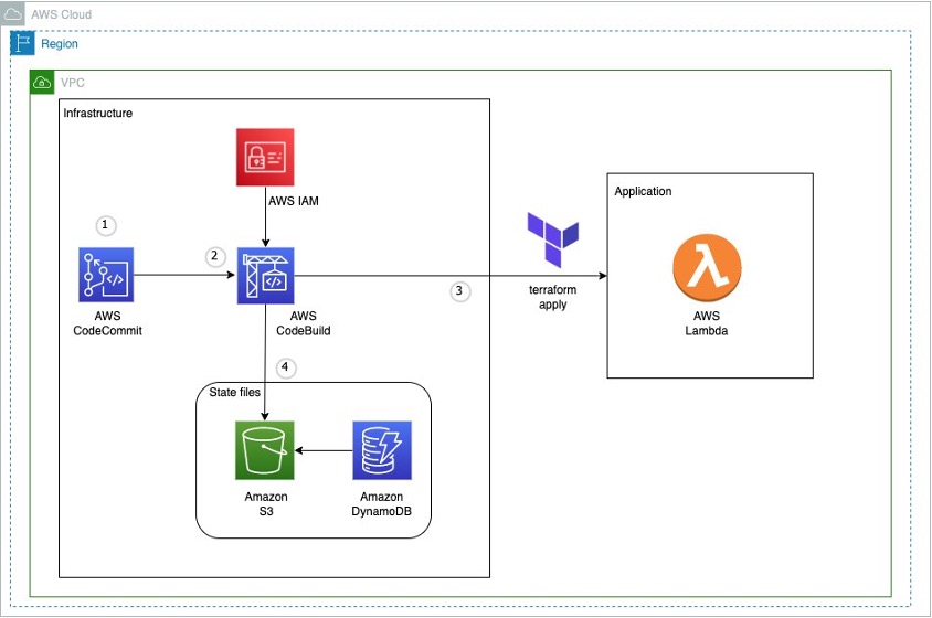
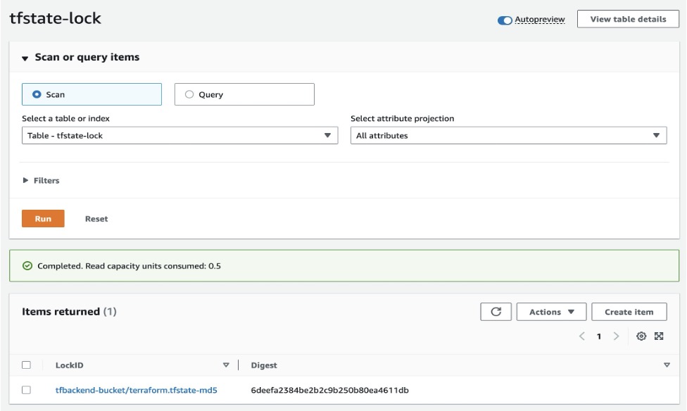
- Apr 2 – Building Serverless Applications with Terraform
- Apr 9 – Developing with Wing Cloud
- Apr 16 – Combining serverless messaging services
- Apr 23 – Real-time web and mobile backends
- Apr 30 – Connecting Confluent to AWS
May
- May 7 – Develop and test locally with LocalStack
- May 14 – Building a personalized GenAI webapp
- May 21 – Serverless GenAI using Bedrock Claude 3
- May 28 – Serverless Platform Engineering
June
- June 4 – Simplifying serverless with the CDK
- June 11 – Learn Serverless with Educloud Academy
- June 18 – Integrating time-series databases
- June 25 – Deploy frontends with the CloudFront Hosting Toolkit
Containers from the Couch

Containers from the Couch
April
May
- May 9 – OPA on AWS
FooBar Serverless

April
- Apr 4 – How to integrate with any service or manual processes with Step Functions?
- Apr 11 – Automating video dubbing with AWS Step Functions and Artificial Intelligence
- Apr 18 – The Future of Solutions Architect: How Generative AI will impact their work?
- Apr 25 – Unveiling the Role of AWS Solutions Architect
February
- May 2 – Understanding the SAGA pattern with AWS Step Functions – With Demo
- May 9 – Working in the cloud – New series!
- May 16 – What does a Software Engineer in the Cloud actually do? | Working in the cloud
- May 23 – How did you get your first job working with cloud computing? | Working in the cloud
- May 30 – From Junior Developer to Cloud Expert | Working in the cloud
June
- Jun 6 – What is your cloud job about? | Working in the cloud
- Jun 13 – Journey to the Cloud | Working in the cloud
- June 27 – Pathways to Cloud Excellence: Insights from Top Industry Experts | Working in the cloud
Still looking for more?
The Serverless landing page has more information. The Lambda resources page contains case studies, webinars, whitepapers, customer stories, reference architectures, and even more Getting Started tutorials.
You can also follow the Serverless Developer Advocacy team on X (formerly Twitter) to see the latest news, follow conversations, and interact with the team.
- Eric Johnson: @edjgeek
- Julian Wood: @julian_wood
- Marcia Villalba: @mavi888uy
- Olly Pomeroy @oliver-p
- Romain Jourdan: @rjourdan_net
And finally, visit the Serverless Land and Containers on AWS websites for all your serverless and serverless container needs.


 Deepak Singh is a Senior Solutions Architect at Amazon Web Services with 20+ years of experience in Data & AIA. He enjoys working with AWS partners and customers on building scalable analytical solutions for their business outcomes. When not at work, he loves spending time with family or exploring new technologies in analytics and AI space.
 Piyush Patra is a Partner Solutions Architect at Amazon Web Services where he supports partners with their Analytics journeys and is the global lead for strategic Data Estate Modernization and Migration partner programs.
 Govind Mohan is an Associate Director with Cognizant with over 18 year of experience in data and analytics space, he has helped design and implement multiple large-scale data migration, application lift & shift and legacy modernization projects and works closely with customers in accelerating the cloud modernization journey leveraging Cognizant Data and Intelligence Toolkit (CDIT) platform.
 Kausik Dhar is a technology leader having more than 23 years of IT experience – primarily focused on Data & Analytics, Data Modernization, Application Development, Delivery Management, and Solution Architecture. He has played a pivotal role in guiding clients through the designing and executing large-scale data and process migrations, in addition to spearheading successful cloud implementations. Kausik possesses expertise in formulating migration strategies for complex programs and adeptly constructing data lake/Lakehouse architecture employing a wide array of tools and technologies.