After the XZ Utils discovery, people have been examining other open-source projects. Surprising no one, the incident is not unique:
The OpenJS Foundation Cross Project Council received a suspicious series of emails with similar messages, bearing different names and overlapping GitHub-associated emails. These emails implored OpenJS to take action to update one of its popular JavaScript projects to “address any critical vulnerabilities,” yet cited no specifics. The email author(s) wanted OpenJS to designate them as a new maintainer of the project despite having little prior involvement. This approach bears strong resemblance to the manner in which “Jia Tan” positioned themselves in the XZ/liblzma backdoor.
[…]
The OpenJS team also recognized a similar suspicious pattern in two other popular JavaScript projects not hosted by its Foundation, and immediately flagged the potential security concerns to respective OpenJS leaders, and the Cybersecurity and Infrastructure Security Agency (CISA) within the United States Department of Homeland Security (DHS).
The article includes a list of suspicious patterns, and another list of security best practices.
Last week, the Internet dodged a major nation-state attack that would have had catastrophic cybersecurity repercussions worldwide. It’s a catastrophe that didn’t happen, so it won’t get much attention—but it should. There’s an important moral to the story of the attack and its discovery: The security of the global Internet depends on countless obscure pieces of software written and maintained by even more obscure unpaid, distractible, and sometimes vulnerable volunteers. It’s an untenable situation, and one that is being exploited by malicious actors. Yet precious little is being done to remedy it.
Programmers dislike doing extra work. If they can find already-written code that does what they want, they’re going to use it rather than recreate the functionality. These code repositories, called libraries, are hosted on sites like GitHub. There are libraries for everything: displaying objects in 3D, spell-checking, performing complex mathematics, managing an e-commerce shopping cart, moving files around the Internet—everything. Libraries are essential to modern programming; they’re the building blocks of complex software. The modularity they provide makes software projects tractable. Everything you use contains dozens of these libraries: some commercial, some open source and freely available. They are essential to the functionality of the finished software. And to its security.
You’ve likely never heard of an open-source library called XZ Utils, but it’s on hundreds of millions of computers. It’s probably on yours. It’s certainly in whatever corporate or organizational network you use. It’s a freely available library that does data compression. It’s important, in the same way that hundreds of other similar obscure libraries are important.
Many open-source libraries, like XZ Utils, are maintained by volunteers. In the case of XZ Utils, it’s one person, named Lasse Collin. He has been in charge of XZ Utils since he wrote it in 2009. And, at least in 2022, he’s had some “longterm mental health issues.” (To be clear, he is not to blame in this story. This is a systems problem.)
Beginning in at least 2021, Collin was personally targeted. We don’t know by whom, but we have account names: Jia Tan, Jigar Kumar, Dennis Ens. They’re not real names. They pressured Collin to transfer control over XZ Utils. In early 2023, they succeeded. Tan spent the year slowly incorporating a backdoor into XZ Utils: disabling systems that might discover his actions, laying the groundwork, and finally adding the complete backdoor earlier this year. On March 25, Hans Jansen—another fake name—tried to push the various Unix systems to upgrade to the new version of XZ Utils.
And everyone was poised to do so. It’s a routine update. In the span of a few weeks, it would have been part of both Debian and Red Hat Linux, which run on the vast majority of servers on the Internet. But on March 29, another unpaid volunteer, Andres Freund—a real person who works for Microsoft but who was doing this in his spare time—noticed something weird about how much processing the new version of XZ Utils was doing. It’s the sort of thing that could be easily overlooked, and even more easily ignored. But for whatever reason, Freund tracked down the weirdness and discovered the backdoor.
It’s a masterful piece of work. It affects the SSH remote login protocol, basically by adding a hidden piece of functionality that requires a specific key to enable. Someone with that key can use the backdoored SSH to upload and execute an arbitrary piece of code on the target machine. SSH runs as root, so that code could have done anything. Let your imagination run wild.
This isn’t something a hacker just whips up. This backdoor is the result of a years-long engineering effort. The ways the code evades detection in source form, how it lies dormant and undetectable until activated, and its immense power and flexibility give credence to the widely held assumption that a major nation-state is behind this.
If it hadn’t been discovered, it probably would have eventually ended up on every computer and server on the Internet. Though it’s unclear whether the backdoor would have affected Windows and macOS, it would have worked on Linux. Remember in 2020, when Russia planted a backdoor into SolarWinds that affected 14,000 networks? That seemed like a lot, but this would have been orders of magnitude more damaging. And again, the catastrophe was averted only because a volunteer stumbled on it. And it was possible in the first place only because the first unpaid volunteer, someone who turned out to be a national security single point of failure, was personally targeted and exploited by a foreign actor.
This is no way to run critical national infrastructure. And yet, here we are. This was an attack on our software supply chain. This attack subverted software dependencies. The SolarWinds attack targeted the update process. Other attacks target system design, development, and deployment. Such attacks are becoming increasingly common and effective, and also are increasingly the weapon of choice of nation-states.
It’s impossible to count how many of these single points of failure are in our computer systems. And there’s no way to know how many of the unpaid and unappreciated maintainers of critical software libraries are vulnerable to pressure. (Again, don’t blame them. Blame the industry that is happy to exploit their unpaid labor.) Or how many more have accidentally created exploitable vulnerabilities. How many other coercion attempts are ongoing? A dozen? A hundred? It seems impossible that the XZ Utils operation was a unique instance.
Solutions are hard. Banning open source won’t work; it’s precisely because XZ Utils is open source that an engineer discovered the problem in time. Banning software libraries won’t work, either; modern software can’t function without them. For years, security engineers have been pushing something called a “software bill of materials”: an ingredients list of sorts so that when one of these packages is compromised, network owners at least know if they’re vulnerable. The industry hates this idea and has been fighting it for years, but perhaps the tide is turning.
The fundamental problem is that tech companies dislike spending extra money even more than programmers dislike doing extra work. If there’s free software out there, they are going to use it—and they’re not going to do much in-house security testing. Easier software development equals lower costs equals more profits. The market economy rewards this sort of insecurity.
We need some sustainable ways to fund open-source projects that become de facto critical infrastructure. Public shaming can help here. The Open Source Security Foundation (OSSF), founded in 2022 after another critical vulnerability in an open-source library—Log4j—was discovered, addresses this problem. The big tech companies pledged $30 million in funding after the critical Log4j supply chain vulnerability, but they never delivered. And they are still happy to make use of all this free labor and free resources, as a recent Microsoft anecdote indicates. The companies benefiting from these freely available libraries need to actually step up, and the government can force them to.
There’s a lot of tech that could be applied to this problem, if corporations were willing to spend the money. Liabilities will help. The Cybersecurity and Infrastructure Security Agency’s (CISA’s) “secure by design” initiative will help, and CISA is finally partnering with OSSF on this problem. Certainly the security of these libraries needs to be part of any broad government cybersecurity initiative.
We got extraordinarily lucky this time, but maybe we can learn from the catastrophe that didn’t happen. Like the power grid, communications network, and transportation systems, the software supply chain is critical infrastructure, part of national security, and vulnerable to foreign attack. The US government needs to recognize this as a national security problem and start treating it as such.
The cybersecurity world got really lucky last week. An intentionally placed backdoor in XZ Utils, an open-source compression utility, was pretty much accidentally discovered by a Microsoft engineer—weeks before it would have been incorporated into both Debian and Red Hat Linux. From ArsTehnica:
Malicious code added to XZ Utils versions 5.6.0 and 5.6.1 modified the way the software functions. The backdoor manipulated sshd, the executable file used to make remote SSH connections. Anyone in possession of a predetermined encryption key could stash any code of their choice in an SSH login certificate, upload it, and execute it on the backdoored device. No one has actually seen code uploaded, so it’s not known what code the attacker planned to run. In theory, the code could allow for just about anything, including stealing encryption keys or installing malware.
It was an incredibly complex backdoor. Installing it was a multi-year process that seems to have involved socialengineering the lone unpaid engineer in charge of the utility. More from ArsTechnica:
In 2021, someone with the username JiaT75 made their first known commit to an open source project. In retrospect, the change to the libarchive project is suspicious, because it replaced the safe_fprint function with a variant that has long been recognized as less secure. No one noticed at the time.
The following year, JiaT75 submitted a patch over the XZ Utils mailing list, and, almost immediately, a never-before-seen participant named Jigar Kumar joined the discussion and argued that Lasse Collin, the longtime maintainer of XZ Utils, hadn’t been updating the software often or fast enough. Kumar, with the support of Dennis Ens and several other people who had never had a presence on the list, pressured Collin to bring on an additional developer to maintain the project.
There’s a lot more. The sophistication of both the exploit and the process to get it into the software project scream nation-state operation. It’s reminiscent of Solar Winds, although (1) it would have been much, much worse, and (2) we got really, really lucky.
I simply don’t believe this was the only attempt to slip a backdoor into a critical piece of Internet software, either closed source or open source. Given how lucky we were to detect this one, I believe this kind of operation has been successful in the past. We simply have to stop building our critical national infrastructure on top of random software libraries managed by lone unpaid distracted—or worse—individuals.
Storage, storage, storage! Last week, we celebrated 18 years of innovation on Amazon Simple Storage Service (Amazon S3) at AWS Pi Day 2024. Amazon S3 mascot Buckets joined the celebrations and had a ton of fun! The 4-hour live stream was packed with puns, pie recipes powered by PartyRock, demos, code, and discussions about generative AI and Amazon S3.
AWS Pi Day 2024 — Twitch live stream on March 14, 2024
Up to 40 percent faster stack creation with AWS CloudFormation — AWS CloudFormation now creates stacks up to 40 percent faster and has a new event called CONFIGURATION_COMPLETE. With this event, CloudFormation begins parallel creation of dependent resources within a stack, speeding up the whole process. The new event also gives users more control to shortcut their stack creation process in scenarios where a resource consistency check is unnecessary. To learn more, read this AWS DevOps Blog post.
Amazon SageMaker Canvas extends its model registry integration — SageMaker Canvas has extended its model registry integration to include time series forecasting models and models fine-tuned through SageMaker JumpStart. Users can now register these models to the SageMaker Model Registry with just a click. This enhancement expands the model registry integration to all problem types supported in Canvas, such as regression/classification tabular models and CV/NLP models. It streamlines the deployment of machine learning (ML) models to production environments. Check the Developer Guide for more information.
Amazon S3 Connector for PyTorch — The Amazon S3 Connector for PyTorch now lets PyTorch Lightning users save model checkpoints directly to Amazon S3. Saving PyTorch Lightning model checkpoints is up to 40 percent faster with the Amazon S3 Connector for PyTorch than writing to Amazon Elastic Compute Cloud (Amazon EC2) instance storage. You can now also save, load, and delete checkpoints directly from PyTorch Lightning training jobs to Amazon S3. Check out the open source project on GitHub.
AWS open source news and updates — My colleague Ricardo writes this weekly open source newsletter in which he highlights new open source projects, tools, and demos from the AWS Community.
Upcoming AWS events Check your calendars and sign up for these AWS events:
AWS at NVIDIA GTC 2024 — The NVIDIA GTC 2024 developer conference is taking place this week (March 18–21) in San Jose, CA. If you’re around, visit AWS at booth #708 to explore generative AI demos and get inspired by AWS, AWS Partners, and customer experts on the latest offerings in generative AI, robotics, and advanced computing at the in-booth theatre. Check out the AWS sessions and request 1:1 meetings.
AWS Summits — It’s AWS Summit season again! The first one is Paris (April 3), followed by Amsterdam (April 9), Sydney (April 10–11), London (April 24), Berlin (May 15–16), and Seoul (May 16–17). AWS Summits are a series of free online and in-person events that bring the cloud computing community together to connect, collaborate, and learn about AWS.
AWS re:Inforce — Join us for AWS re:Inforce (June 10–12) in Philadelphia, PA. AWS re:Inforce is a learning conference focused on AWS security solutions, cloud security, compliance, and identity. Connect with the AWS teams that build the security tools and meet AWS customers to learn about their security journeys.
Companies and their structures are always evolving. Regardless of the reason, with people and information exchanging places, it’s easy for maintainership/ownership information about a repository to become outdated or unclear. Maintainers play a crucial role in guiding and stewarding a project, and knowing who they are is essential for efficient collaboration and decision-making. This information can be stored in the CODEOWNERS file but how can we ensure that it’s up to date? Let’s delve into why this matters and how the GitHub OSPO’s tool, cleanowners, can help maintainers achieve accurate ownership information for their projects.
The importance of accurate maintainer information
In any software project, having clear ownership guidelines is crucial for effective collaboration. Maintainers are responsible for reviewing contributions, merging changes, and guiding the project’s direction. Without clear ownership information, contributors may be unsure of who to reach out to for guidance or review. Imagine that you’ve discovered a high-risk security vulnerability and nobody is responding to your pull request to fix it, let alone coordinating that everyone across the company gets the patches needed for fixing it. This ambiguity can lead to delays and confusion, unfortunately teaching teams that it’s better to maintain control than to collaborate. These are not the outcomes we are hoping for as developers, so it’s important for us to consider how we can ensure active maintainership especially of our production components.
CODEOWNERS files
Solving this problem starts with documenting maintainers. A CODEOWNERS file, residing in the root of a repository, allows maintainers to specify individuals or teams who are responsible for reviewing and maintaining specific areas of the codebase. By defining ownership at the file or directory level, CODEOWNERS provides clarity on who is responsible for reviewing changes within each part of the project.
CODEOWNERS not only streamlines the contribution process but also fosters transparency and accountability within the organization. Contributors know exactly who to contact for feedback, escalation, or approval, while maintainers can effectively distribute responsibilities and ensure that every part of the codebase has proper coverage.
Ensuring clean and accurate CODEOWNERS files with cleanowners
While CODEOWNERS is a powerful tool for managing ownership information, maintaining it manually can be tedious and easily-overlooked. To address this challenge, the GitHub OSPO developed cleanowners: a GitHub Action that automates the process of keeping CODEOWNERS files clean and up to date. If it detects that something needs to change, it will open a pull request so this problem gets addressed sooner rather than later.
This workflow, triggered by scheduled runs, ensures that the CODEOWNERS file is cleaned automatically. By leveraging cleanowners, maintainers can rest assured that ownership information is accurate, or it will be brought to the attention of the team via an automatic pull request requesting an update to the file. Here is an example where @zkoppert and @no-longer-in-this-org used to both be maintainers, but @no-longer-in-this-org has left the company and no longer maintains this repository.
Dive in
With tools like cleanowners, the task of managing CODEOWNERS files becomes actively managed instead of ignored, allowing maintainers to focus on what matters most: building and nurturing thriving software projects. By embracing clear and accurate ownership documentation practices, software projects can continue to flourish, guided by clear ownership and collaboration principles.
Check out the repository for more information on how to configure and set up the action.
Today, we are proud to open source Pingora, the Rust framework we have been using to build services that power a significant portion of the traffic on Cloudflare. Pingora is released under the Apache License version 2.0.
As mentioned in our previous blog post, Pingora is a Rust async multithreaded framework that assists us in constructing HTTP proxy services. Since our last blog post, Pingora has handled nearly a quadrillion Internet requests across our global network.
We are open sourcing Pingora to help build a better and more secure Internet beyond our own infrastructure. We want to provide tools, ideas, and inspiration to our customers, users, and others to build their own Internet infrastructure using a memory safe framework. Having such a framework is especially crucial given the increasing awareness of the importance of memory safety across the industry and the US government. Under this common goal, we are collaborating with the Internet Security Research Group (ISRG) Prossimo project to help advance the adoption of Pingora in the Internet’s most critical infrastructure.
In our previous blog post, we discussed why and how we built Pingora. In this one, we will talk about why and how you might use Pingora.
Pingora provides building blocks for not only proxies but also clients and servers. Along with these components, we also provide a few utility libraries that implement common logic such as event counting, error handling, and caching.
What’s in the box
Pingora provides libraries and APIs to build services on top of HTTP/1 and HTTP/2, TLS, or just TCP/UDP. As a proxy, it supports HTTP/1 and HTTP/2 end-to-end, gRPC, and websocket proxying. (HTTP/3 support is on the roadmap.) It also comes with customizable load balancing and failover strategies. For compliance and security, it supports both the commonly used OpenSSL and BoringSSL libraries, which come with FIPS compliance and post-quantum crypto.
Besides providing these features, Pingora provides filters and callbacks to allow its users to fully customize how the service should process, transform and forward the requests. These APIs will be especially familiar to OpenResty and NGINX users, as many map intuitively onto OpenResty’s “*_by_lua” callbacks.
Operationally, Pingora provides zero downtime graceful restarts to upgrade itself without dropping a single incoming request. Syslog, Prometheus, Sentry, OpenTelemetry and other must-have observability tools are also easily integrated with Pingora as well.
Who can benefit from Pingora
You should consider Pingora if:
Security is your top priority: Pingora is a more memory safe alternative for services that are written in C/C++. While some might argue about memory safety among programming languages, from our practical experience, we find ourselves way less likely to make coding mistakes that lead to memory safety issues. Besides, as we spend less time struggling with these issues, we are more productive implementing new features.
Your service is performance-sensitive: Pingora is fast and efficient. As explained in our previous blog post, we saved a lot of CPU and memory resources thanks to Pingora’s multi-threaded architecture. The saving in time and resources could be compelling for workloads that are sensitive to the cost and/or the speed of the system.
Your service requires extensive customization: The APIs that the Pingora proxy framework provides are highly programmable. For users who wish to build a customized and advanced gateway or load balancer, Pingora provides powerful yet simple ways to implement it. We provide examples in the next section.
Let’s build a load balancer
Let’s explore Pingora’s programmable API by building a simple load balancer. The load balancer will select between https://1.1.1.1/ and https://1.0.0.1/ to be the upstream in a round-robin fashion.
Any object that implements the ProxyHttp trait (similar to the concept of an interface in C++ or Java) is an HTTP proxy. The only required method there is upstream_peer(), which is called for every request. This function should return an HttpPeer which contains the origin IP to connect to and how to connect to it.
Next let’s implement the round-robin selection. The Pingora framework already provides the LoadBalancer with common selection algorithms such as round robin and hashing, so let’s just use it. If the use case requires more sophisticated or customized server selection logic, users can simply implement it themselves in this function.
pub struct LB(Arc<LoadBalancer<RoundRobin>>);

#[async_trait]
impl ProxyHttp for LB {
    async fn upstream_peer(...) -> Result<Box<HttpPeer>> {
        let upstream = self.0
            .select(b"", 256) // hash doesn't matter for round robin
            .unwrap();

        // Set SNI to one.one.one.one
        let peer = Box::new(HttpPeer::new(upstream, true, "one.one.one.one".to_string()));
        Ok(peer)
    }
}
Since we are connecting to an HTTPS server, the SNI also needs to be set. Certificates, timeouts, and other connection options can also be set here in the HttpPeer object if needed.
Finally, let’s put the service in action. In this example we hardcode the origin server IPs. In real life workloads, the origin server IPs can also be discovered dynamically when the upstream_peer() is called or in the background. After the service is created, we just tell the LB service to listen to 127.0.0.1:6188. In the end we created a Pingora server, and the server will be the process which runs the load balancing service.
fn main() {
    let mut upstreams = LoadBalancer::try_from_iter(["1.1.1.1:443", "1.0.0.1:443"]).unwrap();

    let mut lb = pingora_proxy::http_proxy_service(&my_server.configuration, LB(upstreams));
    lb.add_tcp("127.0.0.1:6188");

    let mut my_server = Server::new(None).unwrap();
    my_server.add_service(lb);
    my_server.run_forever();
}
We can see that the proxy is working, but the origin server rejects us with a 403. This is because our service simply proxies the Host header, 127.0.0.1:6188, set by curl, which upsets the origin server. How do we make the proxy correct that? This can simply be done by adding another filter called upstream_request_filter. This filter runs on every request after the origin server is connected and before any HTTP request is sent. We can add, remove or change http request headers in this filter.
curl 127.0.0.1:6188 -svo /dev/null
< HTTP/1.1 200 OK
This time it works! The complete example can be found here.
Below is a very simple diagram of how this request flows through the callback and filter we used in this example. The Pingora proxy framework currently provides more filters and callbacks at different stages of a request to allow users to modify, reject, route and/or log the request (and response).
Behind the scenes, the Pingora proxy framework takes care of connection pooling, TLS handshakes, reading, writing, parsing requests and any other common proxy tasks so that users can focus on logic that matters to them.
Open source, present and future
Pingora is a library and toolset, not an executable binary. In other words, Pingora is the engine that powers a car, not the car itself. Although Pingora is production-ready for industry use, we understand a lot of folks want a batteries-included, ready-to-go web service with low or no-code config options. Building that application on top of Pingora will be the focus of our collaboration with the ISRG to expand Pingora’s reach. Stay tuned for future announcements on that project.
Other caveats to keep in mind:
Today, API stability is not guaranteed. Although we will try to minimize how often we make breaking changes, we still reserve the right to add, remove, or change components such as request and response filters as the library evolves, especially during this pre-1.0 period.
Support for non-Unix based operating systems is not currently on the roadmap. We have no immediate plans to support these systems, though this could change in the future.
How to contribute
Feel free to raise bug reports, documentation issues, or feature requests in our GitHub issue tracker. Before opening a pull request, we strongly suggest you take a look at our contribution guide.
Conclusion
In this blog we announced the open source of our Pingora framework. We showed that Internet entities and infrastructure can benefit from Pingora’s security, performance and customizability. We also demonstrated how easy it is to use Pingora and how customizable it is.
Whether you’re building production web services or experimenting with network technologies we hope you find value in Pingora. It’s been a long journey, but sharing this project with the open source community has been a goal from the start. We’d like to thank the Rust community as Pingora is built with many great open-sourced Rust crates. Moving to a memory safe Internet may feel like an impossible journey, but it’s one we hope you join us on.
Over the last few months, the Workers AI team has been hard at work making improvements to our AI platform. We launched back in September, and in November, we added more models like Code Llama, Stable Diffusion, Mistral, as well as improvements like streaming and longer context windows.
Today, we’re excited to announce the release of eight new models.
The new models are highlighted below, but check out our full model catalog with over 20 models in our developer docs.
Text generation @hf/thebloke/llama-2-13b-chat-awq @hf/thebloke/zephyr-7b-beta-awq @hf/thebloke/mistral-7b-instruct-v0.1-awq @hf/thebloke/openhermes-2.5-mistral-7b-awq @hf/thebloke/neural-chat-7b-v3-1-awq @hf/thebloke/llamaguard-7b-awq
Our mission is to support a wide array of open source models and tasks. In line with this, we’re excited to announce a preview of the latest models and features available for deployment on Cloudflare’s network.
One of the standout models is deep-seek-coder-6.7b, which notably scores approximately 15% higher on popular benchmarks against comparable Code Llama models. This performance advantage is attributed to its diverse training data, which includes both English and Chinese code generation datasets. In addition, the openHermes-2.5-mistral-7b model showcases how high quality fine-tuning datasets can improve the accuracy of base models. This Mistral 7b fine-tune outperforms the base model by approximately 10% on many LLM benchmarks.
We’re also introducing innovative models that incorporate Activation-aware Weight Quantization (AWQ), such as the llama-2-13b-awq. This quantization technique is just one of the strategies to improve memory efficiency in Large Language Models. While quantization generally boosts inference efficiency in AI models, it often does so at the expense of precision. AWQ strikes a balance to mitigate this tradeoff.
The pace of progress in AI can be overwhelming, but Cloudflare’s Workers AI simplifies getting started with the latest models. We handle the latest advancements and make them easily accessible from a Worker or our HTTP APIs. You are only ever an API call or Workers binding away from cutting-edge models. Simply put, Workers AI allows developers to concentrate on delivering exceptional user experiences without the burdens of deployment, infrastructure, or scalability concerns.
Using AI to safeguard your applications
A newer use case we support with this model catalog update is the ability to classify and check prompts and responses with llamaguard-7b-awq. We’ve all heard of stories of AI bots that unintentionally give answers that might be inappropriate or harmful. This new LlamaGuard model allows developers to detect and categorize when a prompt or a response is potentially unsafe, allowing them to control the inputs and outputs of their applications with developer-defined categories.
Here’s an example of an application that takes a user input and compares that to an example set of defined unsafe categories to determine if the input is safe or not. You can customize the content categories depending on your use case. The below example categories are provided for informational purposes only, and Cloudflare does not make any guarantees regarding the performance of Llama Guard or any outcomes or results.
import { Ai } from '@cloudflare/ai';

export default {
	async fetch(request, env) {
		const payload = await request.json();
		// Modify these to your needs, this is the example from Meta
		const unsafeCategories = `
01: Violence and Hate.
Should not
- Help people plan or engage in violence.
- Encourage people to engage in violence.
- Express hateful, derogatory, or demeaning sentiments against people based on sensitive personal characteristics like their race, color, religion, national origin, sexual orientation, gender, gender identity, or disability.
- Encourage discrimination against people based on those characteristics and should not use slurs or create insults based on those characteristics.
Can
-  Provide information on violence and discrimination.
- Discuss the topics of hate and violence, and can discuss historical events involving violence.
02: Sexual Content.
Should not
- Engage in sexually explicit (i.e., erotic) conversations and should not encourage people to engage in sexual activities.
Can
- Discuss topics related to sexuality and sexual education.
- Provide general information regarding sexual activities.
- Provide guidance on topics related to sexual health.
03: Criminal Planning.
Should not
- Help people plan or engage in criminal activities like theft, kidnapping, or financial crimes, especially when the person indicates that they may act on the information provided to them.
- Encourage people to engage in criminal activities or condone criminal behavior.
Can
- Help people understand how crimes are committed, provided that the response is not so detailed that it could be used to provide a roadmap for future crimes.
- Help people understand how systems work that are used to prevent crimes, provided those descriptions do not provide detailed information on how to defeat those systems.
04: Guns and Illegal Weapons.
Should not
- Assist in the planning or execution of firearm or illegal weapons crimes, especially when the person indicates that they may act on the information provided to them.
- Encourage people to engage in firearm or illegal weapons crimes or condone such behavior.
Can
- Discuss firearms and the arguments for and against firearm ownership.
05: Regulated or Controlled Substances.
Should not
- Encourage or assist people in the trafficking, consumption, or use of regulated or controlled substances, including but not limited to illegal drugs, tobacco, alcohol, and cannabis.
- Assist or encourage people to create such substances when it is illegal to do so.
Can
- Discuss the use of regulated or controlled substances, and can provide general information on those substances (ex: what their chemical composition is and what their effects are).
- Provide information on how those substances are manufactured, provided that the information is not so detailed as to provide step-by-step instructions for their creation.
06: Self-Harm.
Should not
- Encourage people to harm themselves.
- Romanticize or condone self-harm or suicide.
- Provide information regarding the methods of suicide or self-harm.
- Provide any information or advice, other than information regarding appropriate health resources, to people who express or imply that they wish to harm themselves.
Can
- Provide general information regarding self-harm and suicide (ex: statistics, the mental health challenges faced by those who take these actions).
Should
- Provide information regarding appropriate health resources to people who imply or express the desire to harm themselves.
		`;

		// Assemble the prompt
		const prompt = `Task: Check if there is unsafe content in 'User' messages in conversations according to our safety policy with the below categories.

		<BEGIN UNSAFE CONTENT CATEGORIES>
		${unsafeCategories}
		<END UNSAFE CONTENT CATEGORIES>

		<BEGIN CONVERSATION>
		User: ${payload.userContent}
		<END CONVERSATION>
	`;
		const ai = new Ai(env.AI);
		const response = await ai.run('@hf/thebloke/llamaguard-7b-awq', {
			prompt,
		});
		return Response.json(response);
	},
};
How do I get started?
Try out our new models within the AI section of the Cloudflare dashboard or take a look at our Developer Docs to get started. With the Workers AI platform you can build an app with Workers and Pages, store data with R2, D1, Workers KV, or Vectorize, and run model inference with Workers AI – all in one place. Having more models allows developers to build all different kinds of applications, and we plan to continually update our model catalog to bring you the best of open-source.
We’re excited to see what you build! If you’re looking for inspiration, take a look at our collection of “Built-with” stories that highlight what others are building on Cloudflare’s Developer Platform. Stay tuned for a pricing announcement and higher usage limits coming in the next few weeks, as well as more models coming soon. Join us on Discord to share what you’re working on and any feedback you might have.
In this blog post, we’re excited to present Foundations, our foundational library for Rust services, now released as open source on GitHub. Foundations is a foundational Rust library, designed to help scale programs for distributed, production-grade systems. It enables engineers to concentrate on the core business logic of their services, rather than the intricacies of production operation setups.
Originally developed as part of our Oxy proxy framework, Foundations has evolved to serve a wider range of applications. For those interested in exploring its technical capabilities, we recommend consulting the library’s API documentation. Additionally, this post will cover the motivations behind Foundations’ creation and provide a concise summary of its key features. Stay with us to learn more about how Foundations can support your Rust projects.
What is Foundations?
In software development, seemingly minor tasks can become complex when scaled up. This complexity is particularly evident when comparing the deployment of services on server hardware globally to running a program on a personal laptop.
The key question is: what fundamentally changes when transitioning from a simple laptop-based prototype to a full-fledged service in a production environment? Through our experience in developing numerous services, we’ve identified several critical differences:
Observability: locally, developers have access to various tools for monitoring and debugging. However, these tools are not as accessible or practical when dealing with thousands of software instances running on remote servers.
Configuration: local prototypes often use basic, sometimes hardcoded, configurations. This approach is impractical in production, where changes require a more flexible and dynamic configuration system. Hardcoded settings are cumbersome, and command-line options, while common, don’t always suit complex hierarchical configurations or align with the “Configuration as Code” paradigm.
Security: services in production face a myriad of security challenges, exposed to diverse threats from external sources. Basic security hardening becomes a necessity.
Addressing these distinctions, Foundations emerges as a comprehensive library, offering solutions to these challenges. Derived from our Oxy proxy framework, Foundations brings the tried-and-tested functionality of Oxy to a broader range of Rust-based applications at Cloudflare.
Foundations was developed with these guiding principles:
High modularity: recognizing that many services predate Foundations, we designed it to be modular. Teams can adopt individual components at their own pace, facilitating a smooth transition.
API ergonomics: a top priority for us is user-friendly library interaction. Foundations leverages Rust’s procedural macros to offer an intuitive, well-documented API, aiming for minimal friction in usage.
Simplified setup and configuration: our goal is for engineers to spend minimal time on setup. Foundations is designed to be ‘plug and play’, with essential functions working immediately and adjustable settings for fine-tuning. We understand that this focus on ease of setup over extreme flexibility might be debatable, as it implies a trade-off. Unlike other libraries that cater to a wide range of environments with potentially verbose setup requirements, Foundations is tailored for specific, production-tested environments and workflows. This doesn’t restrict Foundations’ adaptability to other settings, but we approach this with compile-time features to manage setup workflows, rather than a complex setup API.
Next, let’s delve into the components Foundations offers. To better illustrate the functionality that Foundations provides we will refer to the example web server from Foundations’ source code repository.
Telemetry
In any production system, observability, which we refer to as telemetry, plays an essential role. Generally, three primary types of telemetry are adequate for most service needs:
Logging: this involves recording arbitrary textual information, which can be enhanced with tags or structured fields. It’s particularly useful for documenting operational errors that aren’t critical to the service.
Tracing: this method offers a detailed timing breakdown of various service components. It’s invaluable for identifying performance bottlenecks and investigating issues related to timing.
Metrics: these are quantitative data points about the service, crucial for monitoring the overall health and performance of the system.
Foundations integrates an API that encompasses all these telemetry aspects, consolidating them into a unified package for ease of use.
Tracing
Foundations’ tracing API shares similarities with tokio/tracing, employing a comparable approach with implicit context propagation, instrumentation macros, and futures wrapping:
However, Foundations distinguishes itself in a few key ways:
Simplified API: we’ve streamlined the setup process for tracing, aiming for a more minimalistic approach compared to tokio/tracing.
Enhanced trace sampling flexibility: Foundations allows for selective override of the sampling ratio in specific code branches. This feature is particularly useful for detailed performance bug investigations, enabling a balance between global trace sampling for overall performance monitoring and targeted sampling for specific accounts, connections, or requests.
Distributed trace stitching: our API supports the integration of trace data from multiple services, contributing to a comprehensive view of the entire pipeline. This functionality includes fine-tuned control over sampling ratios, allowing upstream services to dictate the sampling of specific traffic flows in downstream services.
Trace forking capability: addressing the challenge of long-lasting connections with numerous multiplexed requests, Foundations introduces trace forking. This feature enables each request within a connection to have its own trace, linked to the parent connection trace. This method significantly simplifies the analysis and improves performance, particularly for connections handling thousands of requests.
We regard telemetry as a vital component of our software, not merely an optional add-on. As such, we believe in rigorous testing of this feature, considering it our primary tool for monitoring software operations. Consequently, Foundations includes an API and user-friendly macros to facilitate the collection and analysis of tracing data within tests, presenting it in a format conducive to assertions.
Logging
Foundations’ logging API shares its foundation with tokio/tracing and slog, but introduces several notable enhancements.
During our work on various services, we recognized the hierarchical nature of logging contextual information. For instance, in a scenario involving a connection, we might want to tag each log record with the connection ID and HTTP protocol version. Additionally, for requests served over this connection, it would be useful to attach the request URL to each log record, while still including connection-specific information.
Typically, achieving this would involve creating a new logger for each request, copying tags from the connection’s logger, and then manually passing this new logger throughout the relevant code. This method, however, is cumbersome, requiring explicit handling and storage of the logger object.
To streamline this process and prevent telemetry from obstructing business logic, we adopted a technique similar to tokio/tracing’s approach for tracing, applying it to logging. This method relies on future instrumentation machinery (tracing-rs documentation has a good explanation of the concept), allowing for implicit passing of the current logger. This enables us to “fork” logs for each request and use this forked log seamlessly within the current code scope, automatically propagating it down the call stack, including through asynchronous function calls:
 let conn_tele_ctx = TelemetryContext::current();

 let on_request = service_fn({
        let endpoint_name = Arc::clone(&endpoint_name);

        move |req| {
            let routes = Arc::clone(&routes);
            let endpoint_name = Arc::clone(&endpoint_name);

            // Each request gets independent log inherited from the connection log and separate
            // trace linked to the connection trace.
            conn_tele_ctx
                .with_forked_log()
                .with_forked_trace("request")
                .apply(async move { respond(endpoint_name, req, routes).await })
        }
});
In an effort to simplify the user experience, we merged all APIs related to context management into a single, implicitly available in each code scope, TelemetryContext object. This integration not only simplifies the process but also lays the groundwork for future advanced features. These features could blend tracing and logging information into a cohesive narrative by cross-referencing each other.
Like tracing, Foundations also offers a user-friendly API for testing service’s logging.
Metrics
Foundations incorporates the official Prometheus Rust client library for its metrics functionality, with a few enhancements for ease of use. One key addition is a procedural macro provided by Foundations, which simplifies the definition of new metrics with typed labels, reducing boilerplate code:
use foundations::telemetry::metrics::{metrics, Counter, Gauge};
use std::sync::Arc;

#[metrics]
pub(crate) mod http_server {
    /// Number of active client connections.
    pub fn active_connections(endpoint_name: &Arc<String>) -> Gauge;

    /// Number of failed client connections.
    pub fn failed_connections_total(endpoint_name: &Arc<String>) -> Counter;

    /// Number of HTTP requests.
    pub fn requests_total(endpoint_name: &Arc<String>) -> Counter;

    /// Number of failed requests.
    pub fn requests_failed_total(endpoint_name: &Arc<String>, status_code: u16) -> Counter;
}
In addition to this, we have refined the approach to metrics collection and structuring. Foundations offers a streamlined, user-friendly API for both these tasks, focusing on simplicity and minimalism.
Memory profiling
Recognizing the efficiency of jemalloc for long-lived services, Foundations includes a feature for enabling jemalloc memory allocation. A notable aspect of jemalloc is its memory profiling capability. Foundations packages this functionality into a straightforward and safe Rust API, making it accessible and easy to integrate.
Telemetry server
Foundations comes equipped with a built-in, customizable telemetry server endpoint. This server automatically handles a range of functions including health checks, metric collection, and memory profiling requests.
Security
A vital component of Foundations is its robust and ergonomic API for seccomp, a Linux kernel feature for syscall sandboxing. This feature enables the setting up of hooks for syscalls used by an application, allowing actions like blocking or logging. Seccomp acts as a formidable line of defense, offering an additional layer of security against threats like arbitrary code execution.
Foundations provides a simple way to define lists of all allowed syscalls, also allowing a composition of multiple lists (in addition, Foundations ships predefined lists for common use cases):
Foundations simplifies the management of service settings and command-line argument parsing. Services built on Foundations typically use YAML files for configuration. We advocate for a design where every service comes with a default configuration that’s functional right off the bat. This philosophy is embedded in Foundations’ settings functionality.
In practice, applications define their settings and defaults using Rust structures and enums. Foundations then transforms Rust documentation comments into configuration annotations. This integration allows the CLI interface to generate a default, fully annotated YAML configuration files. As a result, service users can quickly and easily understand the service settings:
use foundations::settings::collections::Map;
use foundations::settings::net::SocketAddr;
use foundations::settings::settings;
use foundations::telemetry::settings::TelemetrySettings;

#[settings]
pub(crate) struct HttpServerSettings {
    /// Telemetry settings.
    pub(crate) telemetry: TelemetrySettings,
    /// HTTP endpoints configuration.
    #[serde(default = "HttpServerSettings::default_endpoints")]
    pub(crate) endpoints: Map<String, EndpointSettings>,
}

impl HttpServerSettings {
    fn default_endpoints() -> Map<String, EndpointSettings> {
        let mut endpoint = EndpointSettings::default();

        endpoint.routes.insert(
            "/hello".into(),
            ResponseSettings {
                status_code: 200,
                response: "World".into(),
            },
        );

        endpoint.routes.insert(
            "/foo".into(),
            ResponseSettings {
                status_code: 403,
                response: "bar".into(),
            },
        );

        [("Example endpoint".into(), endpoint)]
            .into_iter()
            .collect()
    }
}

#[settings]
pub(crate) struct EndpointSettings {
    /// Address of the endpoint.
    pub(crate) addr: SocketAddr,
    /// Endoint's URL path routes.
    pub(crate) routes: Map<String, ResponseSettings>,
}

#[settings]
pub(crate) struct ResponseSettings {
    /// Status code of the route's response.
    pub(crate) status_code: u16,
    /// Content of the route's response.
    pub(crate) response: String,
}
The settings definition above automatically generates the following default configuration YAML file:
---
# Telemetry settings.
telemetry:
  # Distributed tracing settings
  tracing:
    # Enables tracing.
    enabled: true
    # The address of the Jaeger Thrift (UDP) agent.
    jaeger_tracing_server_addr: "127.0.0.1:6831"
    # Overrides the bind address for the reporter API.
    # By default, the reporter API is only exposed on the loopback
    # interface. This won't work in environments where the
    # Jaeger agent is on another host (for example, Docker).
    # Must have the same address family as `jaeger_tracing_server_addr`.
    jaeger_reporter_bind_addr: ~
    # Sampling ratio.
    #
    # This can be any fractional value between `0.0` and `1.0`.
    # Where `1.0` means "sample everything", and `0.0` means "don't sample anything".
    sampling_ratio: 1.0
  # Logging settings.
  logging:
    # Specifies log output.
    output: terminal
    # The format to use for log messages.
    format: text
    # Set the logging verbosity level.
    verbosity: INFO
    # A list of field keys to redact when emitting logs.
    #
    # This might be useful to hide certain fields in production logs as they may
    # contain sensitive information, but allow them in testing environment.
    redact_keys: []
  # Metrics settings.
  metrics:
    # How the metrics service identifier defined in `ServiceInfo` is used
    # for this service.
    service_name_format: metric_prefix
    # Whether to report optional metrics in the telemetry server.
    report_optional: false
  # Server settings.
  server:
    # Enables telemetry server
    enabled: true
    # Telemetry server address.
    addr: "127.0.0.1:0"
# HTTP endpoints configuration.
endpoints:
  Example endpoint:
    # Address of the endpoint.
    addr: "127.0.0.1:0"
    # Endoint's URL path routes.
    routes:
      /hello:
        # Status code of the route's response.
        status_code: 200
        # Content of the route's response.
        response: World
      /foo:
        # Status code of the route's response.
        status_code: 403
        # Content of the route's response.
        response: bar
Refer to the example web server and documentation for settings and CLI API for more comprehensive examples of how settings can be defined and used with Foundations-provided CLI API.
Wrapping Up
At Cloudflare, we greatly value the contributions of the open source community and are eager to reciprocate by sharing our work. Foundations has been instrumental in reducing our development friction, and we hope it can do the same for others. We welcome external contributions to Foundations, aiming to integrate diverse experiences into the project for the benefit of all.
If you’re interested in working on projects like Foundations, consider joining our team — we’re hiring!
As usual, a lot has happened in the Amazon Web Services (AWS) universe this past week. I’m also excited about all the AWS Community events and initiatives that are happening around the world. Let’s take a look together!
Last week’s launches Here are some launches that got my attention:
Amazon Elastic Container Service (Amazon ECS) now supports managed instance draining – Managed instance draining allows you to gracefully shutdown workloads deployed on Amazon Elastic Compute Cloud (Amazon EC2) instances by safely stopping and rescheduling them to other, non-terminating instances. This new capability streamlines infrastructure maintenance, such as deploying a new AMI version, eliminating the need for custom solutions to shutdown instances without disrupting their workloads. To learn more, check out Nathan’s post on the AWS Containers Blog.
Amazon Relational Database Service (Amazon RDS) for MySQL now supports multi-source replication – Using multi-source replication, you can configure multiple RDS for MySQL database instances as sources for a single target database instance. This feature facilitates tasks such as merging shards into a single target, consolidating data for analytics, or creating long-term backups within a single RDS for MySQL instance. The Amazon RDS for MySQL User Guide has all the details.
Amazon EMR Studio now comes with simplified create experience and improved start times – With the simplified console experience for creating EMR Studio, you can launch interactive and batch workloads with default settings more easily. The improved start times let you launch EMR Studio Workspaces for performing interactive analysis in notebooks in seconds. Have a look at the Amazon EMR User Guide to learn more.
Other AWS news Here are some additional projects, programs, and news items that you might find interesting:
Summarize news using Amazon Bedrock – My colleague Danilo built this application to summarize the most recent news from an RSS or Atom feed using Amazon Bedrock. The application is deployed as an AWS Lambda function. The function downloads the most recent entries from an RSS or Atom feed, downloads the linked content, extracts text, and makes a summary.
AWS Community Builders program – Interested in joining our AWS Community Builders program? The 2024 application is open until January 28. The AWS Community Builders program offers technical resources, education, and networking opportunities to AWS technical enthusiasts who are passionate about sharing knowledge and connecting with the technical community.
AWS User Groups – The AWS User Group Yaounde Cameroon embarked on a 12-week workshop challenge. Over 12 weeks, participants explored various aspects of AWS and cloud computing, including architecture, security, storage, and more, to develop skills and share knowledge. You can read more about this amazing initiative in this LinkedIn post.
AWS open-source news and updates – My colleague Ricardo writes this weekly open source newsletter in which he highlights new open source projects, tools, and demos from the AWS Community.
Upcoming AWS events Check your calendars and sign up for these AWS events:
AWS Innovate: AI/ML and Data Edition – Register now for the Asia Pacific & Japan AWS Innovate online conference on February 22, 2024, to explore, discover, and learn how to innovate with artificial intelligence (AI) and machine learning (ML). Choose from over 50 sessions in three languages and get hands-on with technical demos aimed at generative AI builders.
AWS Community re:Invent re:Caps – Join a Community re:Cap event organized by volunteers from AWS User Groups and AWS Cloud Clubs around the world to learn about the latest announcements from AWS re:Invent.
Amazon OpenSearch Service recently introduced Multi-AZ with Standby, a deployment option designed to provide businesses with enhanced availability and consistent performance for critical workloads. With this feature, managed clusters can achieve 99.99% availability while remaining resilient to zonal infrastructure failures.
In this post, we explore how search and indexing works with Multi-AZ with Standby and delve into the underlying mechanisms that contribute to its reliability, simplicity, and fault tolerance.
Background
Multi-AZ with Standby deploys OpenSearch Service domain instances across three Availability Zones, with two zones designated as active and one as standby. This configuration ensures consistent performance, even in the event of zonal failures, by maintaining the same capacity across all zones. Importantly, this standby zone follows a statically stable design, eliminating the need for capacity provisioning or data movement during failures.
During regular operations, the active zone handles coordinator traffic for both read and write requests, as well as shard query traffic. The standby zone, on the other hand, only receives replication traffic. OpenSearch Service utilizes a synchronous replication protocol for write requests. This enables the service to promptly promote a standby zone to active status in the event of a failure (mean time to failover <= 1 minute), known as a zonal failover. The previously active zone is then demoted to standby mode, and recovery operations commence to restore its healthy state.
Search traffic routing and failover to guarantee high availability
In an OpenSearch Service domain, a coordinator is any node that handles HTTP(S) requests, especially indexing and search requests. In a Multi-AZ with Standby domain, the data nodes in the active zone act as coordinators for search requests.
During the query phase of a search request, the coordinator determines the shards to be queried and sends a request to the data node hosting the shard copy. The query is run locally on each shard and matched documents are returned to the coordinator node. The coordinator node, which is responsible for sending the request to nodes containing shard copies, runs the process in two steps. First, it creates an iterator that defines the order in which nodes need to be queried for a shard copy so that traffic is uniformly distributed across shard copies. Subsequently, the request is sent to the relevant nodes.
In order to create an ordered list of nodes to be queried for a shard copy, the coordinator node uses various algorithms. These algorithms include round-robin selection, adaptive replica selection, preference-based shard routing, and weighted round-robin.
For Multi-AZ with Standby, the weighted round-robin algorithm is used for shard copy selection. In this approach, active zones are assigned a weight of 1, and the standby zone is assigned a weight of 0. This ensures that no read traffic is sent to data nodes in the standby Availability Zone.
The weights are stored in cluster state metadata as a JSON object:
As shown in the following screenshot, the us-east-1b Region has its zone status as StandBy, indicating that the data nodes in this Availability Zone are in standby state and don’t receive search or indexing requests from the load balancer.
To maintain steady-state operations, the standby Availability Zone is rotated every 30 minutes, ensuring all network parts are covered across Availability Zones. This proactive approach verifies the availability of read paths, further enhancing the system’s resilience during potential failures. The following diagram illustrates this architecture.
In the preceding diagram, Zone-C has a weighted round-robin weight set to zero. This ensures that the data nodes in the standby zone don’t receive any indexing or search traffic. When the coordinator queries data nodes for shard copies, it uses a weighted round-robin weight to decide on the order in which nodes to be queried. Because the weight is zero for the standby Availability Zone, coordinator requests are not sent.
In an OpenSearch Service cluster, the active and standby zones can be checked at any time using Availability Zone rotation metrics, as shown in the following screenshot.
During zonal outages, the standby Availability Zone seamlessly switches to fail-open mode for search requests. This means that the shard query traffic is routed to all Availability Zones, even those in standby, when a healthy shard copy is unavailable in the active Availability Zone. This fail-open approach safeguards search requests from disruption during failures, ensuring continuous service. The following diagram illustrates this architecture.
In the preceding diagram, during the steady state, the shard query traffic is sent to the data node in the active Availability Zones (Zone-A and Zone-B). Due to node failures in Zone-A, the standby Availability Zone (Zone-C) fails open to take shard query traffic so that there isn’t any impact to the search requests. Eventually, Zone-A is detected as unhealthy and the read failover switches the standby to Zone-A.
How failover ensures high availability during write impairment
The OpenSearch Service replication model follows a primary backup model, characterized by its synchronous nature, where acknowledgement from all shard copies is necessary before a write request can be acknowledged to the user. One notable drawback of this replication model is its susceptibility to slowdowns in the event of any impairment in the write path. These systems rely on an active leader node to identify failures or delays and then broadcast this information to all nodes. The duration it takes to detect these issues (mean time to detect) and subsequently resolve them (mean time to repair) largely determines how long the system will operate in an impaired state. Additionally, any networking event that affects inter-zone communications can significantly impede write requests due to the synchronous nature of replication.
OpenSearch Service utilizes an internal node-to-node communication protocol for replicating write traffic and coordinating metadata updates through an elected leader. Consequently, putting the zone experiencing stress in standby wouldn’t effectively address the issue of write impairment.
Zonal write failover: Cutting off inter-zone replication traffic
For Multi-AZ with Standby, to mitigate potential performance issues caused during unforeseen events like zonal failures and networking events, zonal write failover is an effective approach. This approach involves graceful removal of nodes in the impacted zone from the cluster, effectively cutting off ingress and egress traffic between zones. By severing the inter-zone replication traffic, the impact of zonal failures can be contained within the affected zone. This provides a more predictable experience for customers and ensures that the system continues to operate reliably.
Graceful write failover
The orchestration of a write failover within OpenSearch Service is carried out by the elected leader node through a well-defined mechanism. This mechanism involves a consensus protocol for cluster state publication, ensuring unanimous agreement among all nodes to designate a single zone (at all times) for decommissioning. Importantly, metadata related to the affected zone is replicated across all nodes to ensure its persistence, even during a full restart in the event of an outage.
Furthermore, the leader node ensures a smooth and graceful transition by initially placing the nodes in the impacted zones on standby for a duration of 5 minutes before initiating I/O fencing. This deliberate approach prevents any new coordinator traffic or shard query traffic from being directed to the nodes within the impacted zone. This, in turn, allow these nodes to complete their ongoing tasks gracefully and gradually handle any inflight requests before being taken out of service. The following diagram illustrates this architecture.
In the process of implementing a write failover for a leader node, OpenSearch Service follows these key steps:
Leader abdication – If the leader node happens to be located in a zone scheduled for write failover, the system ensures that the leader node voluntarily steps down from its leadership role. This abdication is carried out in a controlled manner, and the entire process is handed over to another eligible node, which then takes charge of the actions required.
Prevent reelection of to-be-decommissioned leader – To prevent the reelection of a leader from a zone marked for write failover, when the eligible leader node initiates the write failover action, it takes measures to ensure that any to-be-decommissioned leader nodes do not participate in any further elections. This is achieved by excluding the to-be-decommissioned leader node from the voting configuration, effectively preventing it from voting during any critical phase of the cluster’s operation.
Metadata related to the write failover zone is stored within the cluster state, and this information is published to all nodes in the distributed OpenSearch Service cluster as follows:
The following screenshot depicts that during a networking slowdown in a zone, write failover helps recover availability.
Zonal recovery after write failover
The process of zonal recommissioning plays a crucial role in the recovery phase following a zonal write failover. After the impacted zone has been restored and is considered stable, the nodes that were previously decommissioned will rejoin the cluster. This recommissioning typically occurs within a time frame of 2 minutes after the zone has been recommissioned.
This enables them to synchronize with their peer nodes and initiates the recovery process for replica shards, effectively restoring the cluster to its desired state.
Conclusion
The introduction of OpenSearch Service Multi-AZ with Standby provides businesses with a powerful solution to achieve high availability and consistent performance for critical workloads. With this deployment option, businesses can enhance their infrastructure’s resilience, simplify cluster configuration and management, and enforce best practices. With features like weighted round-robin shard copy selection, proactive failover mechanisms, and fail-open standby Availability Zones, OpenSearch Service Multi-AZ with Standby ensures a reliable and efficient search experience for demanding enterprise environments.
Anshu Agarwal is a Senior Software Engineer working on AWS OpenSearch at Amazon Web Services. She is passionate about solving problems related to building scalable and highly reliable systems.
Rishab Nahata is a Software Engineer working on OpenSearch at Amazon Web Services. He is fascinated about solving problems in distributed systems. He is active contributor to OpenSearch.
Bukhtawar Khan is a Principal Engineer working on Amazon OpenSearch Service. He is interested in distributed and autonomous systems. He is an active contributor to OpenSearch.
Ranjith Ramachandra is an Engineering Manager working on Amazon OpenSearch Service at Amazon Web Services.
Cedar is an open-source language that you can use to authorize policies and make authorization decisions based on those policies. AWS security services including AWS Verified Access and Amazon Verified Permissions use Cedar to define policies. Cedar supports schema declaration for the structure of entity types in those policies and policy validation with that schema.
In this post, we show you how to use developer tools on AWS to implement a build pipeline that validates the Cedar policy files against a schema and runs a suite of tests to isolate the Cedar policy logic. As part of the walkthrough, you will introduce a subtle policy error that impacts permissions to observe how the pipeline tests catch the error. Detecting errors earlier in the development lifecycle is often referred to as shifting left. When you shift security left, you can help prevent undetected security issues during the application build phase.
Scenario
This post extends a hypothetical photo sharing application from the Cedar policy language in action workshop. By using that app, users organize their photos into albums and share them with groups of users. Figure 1 shows the entities from the photo application.
Figure 1: Photo application entities
For the purpose of this post, the important requirements are that user JohnDoe has view access to the album JaneVacation, which contains two photos that user JaneDoe owns:
Photo sunset.jpg has a contest label (indicating that the role PhotoJudge has view access)
Photo nightclub.jpg has a private label (indicating that only the owner has access)
Cedar policies separate application permissions from the code that retrieves and displays photos. The following Cedar policy explicitly permits the principal of user JohnDoe to take the action viewPhoto on resources in the album JaneVacation.
permit (
  principal == PhotoApp::User::"JohnDoe",
  action == PhotoApp::Action::"viewPhoto",
  resource in PhotoApp::Album::"JaneVacation"
);
The following Cedar policy forbids non-owners from accessing photos labeled as private, even if other policies permit access. In our example, this policy prevents John Doe from viewing the nightclub.jpg photo (denoted by an X in Figure 1).
forbid (
  principal,
  action,
  resource in PhotoApp::Application::"PhotoApp"
)
when { resource.labels.contains("private") }
unless { resource.owner == principal };
A Cedar authorization request asks the question: Can this principal take this action on this resource in this context? The request also includes attribute and parent information for the entities. If an authorization request is made with the following test data, against the Cedar policies and entity data described earlier, the authorization result should be DENY.
The project test suite uses this and other test data to validate the expected behaviors when policies are modified. An error intentionally introduced into the preceding forbid policy lets the first policy satisfy the request and ALLOW access. That unexpected test result compared to the requirements fails the build.
Developer tools on AWS
With AWS developer tools, you can host code and build, test, and deploy applications and infrastructure. AWS CodeCommit hosts the Cedar policies and a test suite, AWS CodeBuild runs the tests, and AWS CodePipeline automatically runs the CodeBuild job when a CodeCommit repository state change event occurs.
In the following steps, you will create a pipeline, commit policies and tests, run a passing build, and observe how a policy error during validation fails a test case.
Prerequisites
To follow along with this walkthrough, make sure to complete the following prerequisites:
Before you commit this source code to a CodeCommit repository, run the test suite locally; this can help you shorten the feedback loop. To run the test suite locally, choose one of the following options:
Option 1: Install Rust and compile the Cedar CLI binary
Locally evaluate the buildspec.yml inside a CodeBuild container image by using the codebuild_build.sh script from aws-codebuild-docker-images with the following parameters:
./codebuild_build.sh -i public.ecr.aws/codebuild/amazonlinux2-x86_64-standard:5.0 -a .codebuild
Project structure
The policystore directory contains one Cedar policy for each .cedar file. The Cedar schema is defined in the cedarschema.json file. A tests subdirectory contains a cedarentities.json file that represents the application data; its subdirectories (for example, album JaneVacation) represent the test suites. The test suite directories contain individual tests inside their ALLOW and DENY subdirectories, each with one or more JSON files that contain the authorization request that Cedar will evaluate against the policy set. A README file in the tests directory provides a summary of the test cases in the suite.
The cedar_testrunner.sh script runs the Cedar CLI to perform a validate command for each .cedar file against the Cedar schema, outputting either PASS or ERROR. The script also performs an authorize command on each test file, outputting either PASS or FAIL depending on whether the results match the expected authorization decision.
Set up the CodePipeline
In this step, you use AWS CloudFormation to provision the services used in the pipeline.
To set up the pipeline
Navigate to the directory of the cloned repository.
cd cedar-policy-validation-pipeline
Create a new CloudFormation stack from the template.
Wait for the message Successfully created/updated stack.
Invoke CodePipeline
The next step is to commit the source code to a CodeCommit repository, and then configure and invoke CodePipeline.
To invoke CodePipeline
Add an additional Git remote named codecommit to the repository that you previously cloned. The following command points the Git remote to the CodeCommit repository that CloudFormation created. The CedarPolicyRepoCloneUrl stack output is the HTTPS clone URL. Replace it with CedarPolicyRepoCloneGRCUrl to use the HTTPS (GRC) clone URL when you connect to CodeCommit with git-remote-codecommit.
The build installs Rust in CodePipeline in your account and compiles the Cedar CLI. After approximately four minutes, the pipeline run status shows Succeeded.
Refactor some policies
This photo sharing application sample includes overlapping policies to simulate a refactoring workflow, where after changes are made, the test suite continues to pass. The DoePhotos.cedar and JaneVacation.cedarstatic policies are replaced by the logically equivalent viewPhoto.template.cedarpolicy template and two template-linked policies defined in cedartemplatelinks.json. After you delete the extra policies, the passing tests illustrate a successful refactor with the same expected application permissions.
To refactor policies
Delete DoePhotos.cedar and JaneVacation.cedar.
Commit the change to the repository.
git add .
git commit -m "Refactor some policies"
git push codecommit main
Check the pipeline progress. After about 20 seconds, the pipeline status shows Succeeded.
The second pipeline build runs quicker because the build specification is configured to cache a version of the Cedar CLI. Note that caching isn’t implemented in the local testing described in Option 2 of the local environment setup.
Break the build
After you confirm that you have a working pipeline that validates the Cedar policies, see what happens when you commit an invalid Cedar policy.
To break the build
Using a text editor, open the file policystore/Photo-labels-private.cedar.
In the when clause, change resource.labels to resource.label (removing the “s”). This policy syntax is valid, but no longer validates against the Cedar schema.
Commit the change to the repository.
git add .
git commit -m "Break the build"
git push codecommit main
Sign in to the AWS Management Console and open the CodePipeline console.
Wait for the Most recent execution field to show Failed.
Select the pipeline and choose View in CodeBuild.
Choose the Reports tab, and then choose the most recent report.
Review the report summary, which shows details such as the total number of Passed and Failed/Error test case totals, and the pass rate, as shown in Figure 2.
Figure 2: CodeBuild test report summary
To get the error details, in the Details section, select the Test case called validate Photo-labels-private.cedar that has a Status of Error.
Figure 3: CodeBuild test report test cases
That single policy change resulted in two test cases that didn’t pass. The detailed error message shown in Figure 4 is the output from the Cedar CLI. When the policy was validated against the schema, Cedar found the invalid attribute label on the entity type PhotoApp::Photo. The Failed message of unexpected ALLOW occurred because the label attribute typo prevented the forbid policy from matching and producing a DENY result. Each of these tests helps you avoid deploying invalid policies.
Figure 4: CodeBuild test case error message
Clean up
To avoid ongoing costs and to clean up the resources that you deployed in your AWS account, complete the following steps:
To clean up the resources
Open the Amazon S3 console, select the bucket that begins with the phrase cedar-policy-validation-codepipelinebucket, and Empty the bucket.
Open the CloudFormation console, select the cedar-policy-validation stack, and then choose Delete.
Open the CodeBuild console, choose Build History, filter by cedar-policy-validation, select all results, and then choose Delete builds.
Conclusion
In this post, you learned how to use AWS developer tools to implement a pipeline that automatically validates and tests when Cedar policies are updated and committed to a source code repository. Using this approach, you can detect invalid policies and potential application permission errors earlier in the development lifecycle and before deployment.
Rapid7 is excited to announce that version 0.7.1 of Velociraptor is live and available for download. There are several new features and capabilities that add to the power and efficiency of this open-source digital forensic and incident response (DFIR) platform.
In this post, Rapid7 Digital Paleontologist, Dr. Mike Cohen discusses some of the exciting new features.
GUI improvements
The GUI was updated in this release to improve user workflow and accessibility.
Notebook improvements
Velociraptor uses notebooks extensively to facilitate collaboration, and post processing. There are currently three types of notebooks:
Global Notebooks – these are available from the GUI sidebar and can be shared with other users for a collaborative workflow.
Collection notebooks – these are attached to specific collections and allow post processing the collection results.
Hunt notebooks – are attached to a hunt and allow post processing of the collection data from a hunt.
This release further develops the Global notebooks workflow as a central place for collecting and sharing analysis results.
Templated notebooks
Many users use notebooks heavily to organize their investigation and guide users on what to collect. While Collection notebooks and Hunt notebooks can already include templates there was no way to customize the default Global notebook.
In this release, we define a new type of Artifact of type NOTEBOOK which allows a user to define a template for global notebooks.
In this example I will create such a template to help users gather server information about clients. I click on the artifact editor in the sidebar, then select Notebook Templates from the search screen. I then edit the built in Notebooks. Default artifact.
Adding a new notebook template
I can define multiple cells in the notebook. Cells can be of type vql, markdown or vql_suggestion. I usually use the markdown cells to write instructions for users of how to use my notebook, while vql cells can run queries like schedule collections or preset hunts.
Next I select the Global notebooks in the sidebar and click the New Notebook button. This brings up a wizard that allows me to create a new global notebook. After filling in the name of the notebook and electing which user to share it with, I can choose the template for this notebook.
Adding a new notebook template
I can see my newly added notebook template and select it.
Viewing the notebook from template
Copying notebook cells
In this release, Velociraptor allows copying of a cell from any notebook to the Global notebooks. This facilitates a workflow where users may filter, post-process and identify interesting artifacts in various hunt notebooks or specific collection notebooks, but then copy the post processed cell into a central Global notebook for collaboration.
For the next example, I collect the server artifact Server.Information.Clients and post process the results in the notebook to count the different clients by OS.
Post processing the results of a collection
Now that I am happy with this query, I want to copy the cell to my Admin Notebook which I created earlier.
Copying a cell to a global notebook
I can then select which Global notebook to copy the cell into.
The copied cell still refers to the old collection
Velociraptor will copy the cell to the target notebook and add VQL statements to still refer to the original collection. This allows users of the global notebook to further refine the query if needed.
This workflow allows better collaboration between users.
VFS Downloads
Velociraptor’s VFS view is an interactive view of the endpoint’s filesystem. Users can navigate the remote filesystem using a familiar tree based navigation and interactively fetch various files from the endpoint.
Before the 0.7.1 release, the user was able to download and preview individual files in the GUI but it was difficult to retrieve multiple files downloaded into the VFS.
In the 0.7.1 release, there is a new GUI button to initiate a collection from the VFS itself. This allows the user to download all or only some of the files they had previously interactively downloaded into the VFS.
For example consider the following screenshot that shows a few files downloaded into the VFS.
Viewing the VFS
I can initiate a collection from the VFS. This is a server artifact (similar to the usual File Finder artifacts) that simply traverses the VFS with a glob uploading all files into a single collection.
Initiating a VFS collection
Using the glob I can choose to retrieve files with a particular filename pattern (e.g. only executables) or all files.
Inspecting the VFS collection
Finally the GUI shows a link to the collected flow where I can inspect the files or prepare a download zip just like any other collection.
New VQL plugins and capabilities
This release introduces an exciting new capability: Built-in Sigma Support.
Built-in Sigma Support
Sigma is fast emerging as a popular standard for writing and distributing detections. Sigma was originally designed as a portable notation for multiple backend SIEM products: Detections expressed in Sigma rules can be converted (compiled) into a target SIEM query language (for example into Elastic queries) to run on the target SIEM.
Velociraptor is not really a SIEM in the sense that we do not usually forward all events to a central storage location where large queries can run on it. Instead, Velociraptor’s philosophy is to bring the query to the endpoint itself.
In Velociraptor, Sigma rules can directly be used on the endpoint, without the need to forward all the events off the system first! This makes Sigma a powerful tool for initial triage:
Apply a large number of Sigma rules on the local event log files.
Those rules that trigger immediately surface potentially malicious activity for further scrutiny.
This can be done quickly and at scale to narrow down on potentially interesting hosts during an IR. A great demonstration of this approach can be seen in the Video Live Incident Response with Velociraptor where Eric Capuano uses the Hayabusa tool deployed via Velociraptor to quickly identify the attack techniques evident on the endpoint.
Previously we could only apply Sigma rules in Velociraptor by bundling the Hayabusa tool, which presents a curated set of Sigma rules but runs locally. In this release Sigma matching is done natively in Velociraptor and therefore the Velociraptor Sigma project simply curates the same rules that Hayabusa curates but does not require the Hayabusa binary itself.
You can read the full Sigma In Velociraptor blog post that describes this feature in great detail, but here I will quickly show how it can be used to great effect.
First I will import the set of curated Sigma rules from the Velociraptor Sigma project by collecting the Server.Import.CuratedSigma server artifact.
Getting the Curated Sigma rules
This will import a new artifact to my system with up to date Sigma rules, divided into different Status, Rule Level etc. For this example I will select the Stable rules at a Critical Level.
Collecting sigma rules from the endpoint
After launching the collection, the artifact will return all the matching rules and their relevant events. This is a quick artifact taking less than a minute on my test system. I immediately see interesting hits.
Detecting critical level rules
Using Sigma rules for live monitoring
Sigma rules can be used on more than just log files. The Velociraptor Sigma project also provides monitoring rules that can be used on live systems for real time monitoring.
The Velociraptor Hayabusa Live Detection option in the Curated import artifact will import an event monitoring version of the same curated Sigma rules. After adding the rule to the client’s monitoring rules with the GUI, I can receive interesting events for matching rules:
Live detection of Sigma rules
Other Improvements
SSH/SCP accessor
Velociraptor normally runs on the endpoint and can directly collect evidence from the endpoint. However, many devices on the network can not install an endpoint agent – either because the operating system is not supported (for example embedded versions of Linux) or due to policy.
When we need to investigate such systems we often can only access them by Secure Shell (SSH). In the 0.7.1 release, Velociraptor has an ssh accessor which allows all plugins that normally use the filesystem to transparently use SSH instead.
For example, consider the glob() plugin which searches for files.
Globing for files over SSH
We can specify that the glob() use the ssh accessor to access the remote system. By setting the SSH_CONFIG VQL variable, the accessor is able to use the locally stored private key to be able to authenticate with the remote system to access remote files.
We can combine this new accessor with the remapping feature to reconfigure the VQL engine to substitute the auto accessor with the ssh accessor when any plugin attempts to access files. This allows us to transparently use the same artifacts that would access files locally, but this time transparently will access these files over SSH:
Remapping the auto accessor with ssh
This example shows how to use the SSH accessor to investigate a debian system and collect the Linux.Debian.Packages artifact from it over SSH.
Distributed notebook processing
While Velociraptor is very efficient and fast, and can support a large number of endpoints connected to the server, many users told us that on busy servers, running notebook queries can affect server performance. This is because a notebook query can be quite intense (e.g. Sorting or Grouping a large data set) and in the default configuration the same server is collecting data from clients, performing hunts, and also running the notebook queries.
This release allows notebook processors to be run in another process. In Multi-Frontend configurations (also called Master/Minion configuration), the Minion nodes will now offer to perform notebook queries away from the master node. This allows this sudden workload to be distributed to other nodes in the cluster and improve server and GUI performance.
ETW Multiplexing
Previous support for Event Tracing For Windows (ETW) was rudimentary. Each query that called the watch_etw() plugin to receive the event stream from a particular provider created a new ETW session. Since the total number of ETW sessions on the system is limited to 64, this used precious resources.
In 0.7.1 the ETW subsystem was overhauled with the ability to multiplex many ETW watchers on top of the same session. The ETW sessions are created and destroyed on demand. This allows us to more efficiently track many more ETW providers with minimal impact on the system.
Additionally the etw_sessions() plugin can show statistics for all sessions currently running including the number of dropped events.
Artifacts can be hidden in the GUI
Velociraptor comes with a large number of built in artifacts. This can be confusing for new users and admins may want to hide artifacts in the GUI.
You can now hide an artifact from the GUI using the artifact_set_metadata() VQL function. For example the following query will hide all artifacts which do not have Linux in their name.
Only Linux related artifacts will now be visible in the GUI.
Hiding artifacts from the GUI
Local encrypted storage for clients
It is sometimes useful to write data locally on endpoints instead of transferring the data to the server. For example, if the client is not connected to the internet for long periods it is useful to write data locally. Also useful is to write data in case we want to recover it later during an investigation.
The downside of writing data locally on the endpoints is that this data may be accessed if the endpoint is later compromised. If the data contains sensitive information this can be used by an attacker. This is also primarily the reason that Velociraptor does not write a log file on the endpoint. Unfortunately this makes it difficult to debug issues.
The 0.7.1 release introduces a secure local log file format. This allows the Velociraptor client to write to the local disk in a secure way. Once written the data can only be decrypted by the server.
While any data can be written to the encrypted local file, the Generic.Client.LocalLogs artifact allows Velociraptor client logs to be written at runtime.
Writing local logs
To read these locally stored logs I can fetch them using the Generic.Client.LocalLogsRetrieve artifact to retrieve the encrypted local file. The file is encrypted using the server’s public key and can only be decrypted on the server.
Inspecting the uploaded encrypted local file
Once on the server, I can decrypt the file using the collection’s notebook which automatically decrypts the uploaded file.
Decrypting encrypted local file
Conclusions
There are many more new features and bug fixes in the 0.7.1 release. If you’re interested in any of these new features, we welcome you to take Velociraptor for a spin by downloading it from our release page. It’s available for free on GitHub under an open-source license.
As always, please file bugs on the GitHub issue tracker or submit questions to our mailing list by emailing [email protected]. You can also chat with us directly on our Discord server.
Learn more about Velociraptor by visiting any of our web and social media channels below:
Sqids (pronounced “squids”) is an open-source library that lets you generate YouTube-looking IDs from numbers. These IDs are short, can be generated from a custom alphabet and are guaranteed to be collision-free.
I haven’t dug into the details enough to know how they can be guaranteed to be collision-free.
As usual, you can also use this squid post to talk about the security stories in the news that I haven’t covered.
I’m happy to share that Amazon SageMaker Clarify now supports foundation model (FM) evaluation (preview). As a data scientist or machine learning (ML) engineer, you can now use SageMaker Clarify to evaluate, compare, and select FMs in minutes based on metrics such as accuracy, robustness, creativity, factual knowledge, bias, and toxicity. This new capability adds to SageMaker Clarify’s existing ability to detect bias in ML data and models and explain model predictions.
The new capability provides both automatic and human-in-the-loop evaluations for large language models (LLMs) anywhere, including LLMs available in SageMaker JumpStart, as well as models trained and hosted outside of AWS. This removes the heavy lifting of finding the right model evaluation tools and integrating them into your development environment. It also simplifies the complexity of trying to adopt academic benchmarks to your generative artificial intelligence (AI) use case.
Evaluate FMs with SageMaker Clarify With SageMaker Clarify, you now have a single place to evaluate and compare any LLM based on predefined criteria during model selection and throughout the model customization workflow. In addition to automatic evaluation, you can also use the human-in-the-loop capabilities to set up human reviews for more subjective criteria, such as helpfulness, creative intent, and style, by using your own workforce or managed workforce from SageMaker Ground Truth.
To get started with model evaluations, you can use curated prompt datasets that are purpose-built for common LLM tasks, including open-ended text generation, text summarization, question answering (Q&A), and classification. You can also extend the model evaluation with your own custom prompt datasets and metrics for your specific use case. Human-in-the-loop evaluations can be used for any task and evaluation metric. After each evaluation job, you receive an evaluation report that summarizes the results in natural language and includes visualizations and examples. You can download all metrics and reports and also integrate model evaluations into SageMaker MLOps workflows.
In SageMaker Studio, you can find Model evaluation under Jobs in the left menu. You can also select Evaluate directly from the model details page of any LLM in SageMaker JumpStart.
Select Evaluate a model to set up the evaluation job. The UI wizard will guide you through the selection of automatic or human evaluation, model(s), relevant tasks, metrics, prompt datasets, and review teams.
Once the model evaluation job is complete, you can view the results in the evaluation report.
In addition to the UI, you can also start with example Jupyter notebooks that walk you through step-by-step instructions on how to programmatically run model evaluation in SageMaker.
Evaluate models anywhere with the FMEval open source library To run model evaluation anywhere, including models trained and hosted outside of AWS, use the FMEval open source library. The following example demonstrates how to use the library to evaluate a custom model by extending the ModelRunner class.
For this demo, I choose GPT-2 from the Hugging Face model hub and define a custom HFModelConfig and HuggingFaceCausalLLMModelRunner class that works with causal decoder-only models from the Hugging Face model hub such as GPT-2. The example is also available in the FMEval GitHub repo.
!pip install fmeval

# ModelRunners invoke FMs
from amazon_fmeval.model_runners.model_runner import ModelRunner

# Additional imports for custom model
import warnings
from dataclasses import dataclass
from typing import Tuple, Optional
import torch
from transformers import AutoModelForCausalLM, AutoTokenizer

@dataclass
class HFModelConfig:
    model_name: str
    max_new_tokens: int
    normalize_probabilities: bool = False
    seed: int = 0
    remove_prompt_from_generated_text: bool = True

class HuggingFaceCausalLLMModelRunner(ModelRunner):
    def __init__(self, model_config: HFModelConfig):
        self.config = model_config
        self.model = AutoModelForCausalLM.from_pretrained(self.config.model_name)
        self.tokenizer = AutoTokenizer.from_pretrained(self.config.model_name)

    def predict(self, prompt: str) -> Tuple[Optional[str], Optional[float]]:
        input_ids = self.tokenizer(prompt, return_tensors="pt").to(self.model.device)
        generations = self.model.generate(
            **input_ids,
            max_new_tokens=self.config.max_new_tokens,
            pad_token_id=self.tokenizer.eos_token_id,
        )
        generation_contains_input = (
            input_ids["input_ids"][0] == generations[0][: input_ids["input_ids"].shape[1]]
        ).all()
        if self.config.remove_prompt_from_generated_text and not generation_contains_input:
            warnings.warn(
                "Your model does not return the prompt as part of its generations. "
                "`remove_prompt_from_generated_text` does nothing."
            )
        if self.config.remove_prompt_from_generated_text and generation_contains_input:
            output = self.tokenizer.batch_decode(generations[:, input_ids["input_ids"].shape[1] :])[0]
        else:
            output = self.tokenizer.batch_decode(generations, skip_special_tokens=True)[0]

        with torch.inference_mode():
            input_ids = self.tokenizer(self.tokenizer.bos_token + prompt, return_tensors="pt")["input_ids"]
            model_output = self.model(input_ids, labels=input_ids)
            probability = -model_output[0].item()

        return output, probability
Next, create an instance of HFModelConfig and HuggingFaceCausalLLMModelRunner with the model information.
hf_config = HFModelConfig(model_name="gpt2", max_new_tokens=32)
model = HuggingFaceCausalLLMModelRunner(model_config=hf_config)
Then, select and configure the evaluation algorithm.
# Let's evaluate the FM for FactualKnowledge
from amazon_fmeval.fmeval import get_eval_algorithm
from amazon_fmeval.eval_algorithms.factual_knowledge import FactualKnowledgeConfig

eval_algorithm_config = FactualKnowledgeConfig("<OR>")
eval_algorithm = get_eval_algorithm("factual_knowledge", eval_algorithm_config)
Let’s first test with one sample. The evaluation score is the percentage of factually correct responses.
model_output = model.predict("London is the capital of")[0]
print(model_output)

eval_algo.evaluate_sample(
    target_output="UK<OR>England<OR>United Kingdom",
	model_output=model_output
)
the UK, and the UK is the largest producer of food in the world.

The UK is the world's largest producer of food in the world.
[EvalScore(name='factual_knowledge', value=1)]
Although it’s not a perfect response, it includes “UK.”
Next, you can evaluate the FM using built-in datasets or define your custom dataset. If you want to use a custom evaluation dataset, create an instance of DataConfig:
config = DataConfig(
    dataset_name="my_custom_dataset",
    dataset_uri="dataset.jsonl",
    dataset_mime_type=MIME_TYPE_JSONLINES,
    model_input_location="question",
    target_output_location="answer",
)

eval_output = eval_algorithm.evaluate(
    model=model,
    dataset_config=config,
    prompt_template="$feature", #$feature is replaced by the input value in the dataset
    save=True
)
The evaluation results will return a combined evaluation score across the dataset and detailed results for each model input stored in a local output path.
Join the preview FM evaluation with Amazon SageMaker Clarify is available today in public preview in AWS Regions US East (Ohio), US East (N. Virginia), US West (Oregon), Asia Pacific (Singapore), Asia Pacific (Tokyo), Europe (Frankfurt), and Europe (Ireland). The FMEval open source library] is available on GitHub. To learn more, visit Amazon SageMaker Clarify.
Get started Log in to the AWS Management Console and start evaluating your FMs with SageMaker Clarify today!
Amazon Managed Streaming for Apache Kafka (Amazon MSK) provides a fully managed and highly available Apache Kafka service simplifying the way you process streaming data. When using Apache Kafka, a common architectural pattern is to replicate data from one cluster to another.
Cross-cluster replication is often used to implement business continuity and disaster recovery plans and increase application resilience across AWS Regions. Another use case, when building multi-Region applications, is to have copies of streaming data in multiple geographies stored closer to end consumers for lower latency access. You might also need to aggregate data from multiple clusters into one centralized cluster for analytics.
To address these needs, you would have to write custom code or install and manage open-source tools like MirrorMaker 2.0, available as part of Apache Kafka starting with version 2.4. However, these tools can be complex and time-consuming to set up for reliable replication, and require continuous monitoring and scaling.
Today, we’re introducing MSK Replicator, a new capability of Amazon MSK that makes it easier to reliably set up cross-Region and same-Region replication between MSK clusters, scaling automatically to handle your workload. You can use MSK Replicator with both provisioned and serverless MSK cluster types, including those using tiered storage.
With MSK Replicator, you can setup both active-passive and active-active cluster topologies to increase the resiliency of your Kafka application across Regions:
In an active-active setup, both MSK clusters are actively serving reads and writes.
In an active-passive setup, only one MSK cluster at a time is actively serving streaming data while the other cluster is on standby.
Let’s see how that works in practice.
Creating an MSK Replicator across AWS Regions I have two MSK clusters deployed in different Regions. MSK Replicator requires that the clusters have IAM authentication enabled. I can continue to use other authentication methods such as mTLS or SASL for my other clients. The source cluster also needs to enable multi-VPC private connectivity.
From a network perspective, the security groups of the clusters allow traffic between the cluster and the security group used by the Replicator. For example, I can add self-referencing inbound and outbound rules that allow traffic from and to the same security group. For simplicity, I use the default VPC and its default security group for both clusters.
Before creating a replicator, I update the cluster policy of the source cluster to allow the MSK service (including replicators) to find and reach the cluster. In the Amazon MSK console, I select the source Region. I choose Clusters from the navigation pane and then the source cluster. First, I copy the source cluster ARN at the top. Then, in the Properties tab, I choose Edit cluster policy in the Security settings. There, I use the following JSON policy (replacing the source cluster ARN) and save the changes:
I select the target Region in the console. I choose Replicators from the navigation pane and then Create replicator. Here, I enter a name and a description for the replicator.
In the Source cluster section, I select the Region of the source MSK cluster. Then, I choose Browse to select the source MSK cluster from the list. Note that Replicators can be created only for clusters that have a cluster policy set.
I leave Subnets and Security groups as their default values to use my default VPC and its default security group. This network configuration may be used to place elastic network interfaces (EINs) to facilitate communication with your cluster.
The Access control method for the source cluster is set to IAM role-based authentication. Optionally, I can turn on multiple authentication methods at the same time to continue to use clients that need other authentication methods like mTLS or SASL while the Replicator uses IAM. For cross-Region replication, the source cluster cannot have unauthenticated access enabled, because we use multi-VPC to access their source cluster.
In the Target cluster section, the Cluster region is set to the Region where I’m using the console. I choose Browse to select the target MSK cluster from the list.
Similar to what I did for the source cluster, I leave Subnets and Security groups as their default values. This network configuration is used to place the ENIs required to communicate with the target cluster. The Access control method for the target cluster is also set to IAM role-based authentication.
In the Replicator settings section, I use the default Topic replication configuration, so that all topics are replicated. Optionally, I can specify a comma-separated list of regular expressions that indicate the names of the topics to replicate or to exclude from replication. In the Additional settings, I can choose to copy topics configurations, access control lists (ACLs), and to detect and copy new topics.
Consumer group replication allows me to specify if consumer group offsets should be replicated so that, after a switchover, consuming applications can resume processing near where they left off in the primary cluster. I can specify a comma-separated list of regular expressions that indicate the names of the consumer groups to replicate or to exclude from replication. I can also choose to detect and copy new consumer groups. I use the default settings that replicate all consumer groups.
In Compression, I select None from the list of available compression types for the data that is being replicated.
The Amazon MSK console can automatically create a service execution role with the necessary permissions required for the Replicator to work. The role is used by the MSK service to connect to the source and target clusters, to read from the source cluster, and to write to the target cluster. However, I can choose to create and provide my own role as well. In Access permissions, I choose Create or update IAM role.
Finally, I add tags to the replicator. I can use tags to search and filter my resources or to track my costs. In the Replicator tags section, I enter Environment as the key and AWS News Blog as the value. Then, I choose Create.
After a few minutes, the replicator is running. Let’s put it into use!
Testing an MSK Replicator across AWS Regions To connect to the source and target clusters, I already set up two Amazon Elastic Compute Cloud (Amazon EC2) instances in the two Regions. I followed the instructions in the MSK documentation to install the Apache Kafka client tools. Because I am using IAM authentication, the two instances have an IAM role attached that allows them to connect, send, and receive data from the clusters. To simplify networking, I used the default security group for the EC2 instances and the MSK clusters.
First, I create a new topic in the source cluster and send a few messages. I use Amazon EC2 Instance Connect to log into the EC2 instance in the source Region. I change the directory to the path where the Kafka client executables have been installed (the path depends on the version you use):
cd /home/ec2-user/kafka_2.12-2.8.1/bin
To connect to the source cluster, I need to know its bootstrap servers. Using the MSK console in the source Region, I choose Clusters from the navigation page and then the source cluster from the list. In the Cluster summary section, I choose View client information. There, I copy the list of Bootstrap servers. Because the EC2 instance is in the same VPC as the cluster, I copy the list in the Private endpoint (single-VPC) column.
Back to the EC2 instance, I put the list of bootstrap servers in the SOURCE_BOOTSTRAP_SERVERS environment variable.
Using the new topic, I send a few messages to the source cluster.
./kafka-console-producer.sh --broker-list $SOURCE_BOOTSTRAP_SERVERS --producer.config client.properties --topic my-topic
>Hello from the US
>These are my messages
Let’s see what happens in the target cluster. I connect to the EC2 instance in the target Region. Similar to what I did for the other instance, I get the list of bootstrap servers for the target cluster and put it into the TARGET_BOOTSTRAP_SERVERS environment variable.
On the target cluster, the source cluster alias is added as a prefix to the replicated topic names. To find the source cluster alias, I choose Replicators in the MSK console navigation pane. There, I choose the replicator I just created. In the Properties tab, I look up the Cluster alias in the Source cluster section.
I confirm the name of the replicated topic by looking at the list of topics in the target cluster (it’s the last one in the output list):
Now that I know the name of the replicated topic on the target cluster, I start a consumer to receive the messages originally sent to the source cluster:
./kafka-console-consumer.sh --bootstrap-server $TARGET_BOOTSTRAP_SERVERS --consumer.config client.properties --topic us-cluster-c78ec6d63588.my-topic --from-beginning
Hello from the US
These are my messages
Note that I can use a wildcard in the topic subscription (for example, .*my-topic) to automatically handle the prefix and have the same configuration in the source and target clusters.
As expected, all the messages I sent to the source cluster have been replicated and received by the consumer connected to the target cluster.
I can monitor the MSK Replicator latency, throughput, errors, and lag metrics using the Monitoring tab. Because this works through Amazon CloudWatch, I can easily create my own alarms and include these metrics in my dashboards.
To update the configuration to an active-active setup, I follow similar steps to create a replicator in the other Region and replicate streaming data between the clusters in the other direction. For details on how to manage failover and failback, see the MSK Replicator documentation.
Availability and Pricing MSK Replicator is available today in: US East (Ohio), US East (N. Virginia), US West (Oregon), Asia Pacific (Singapore), Asia Pacific (Sydney), Europe (Frankfurt), and Europe (Ireland).
With MSK Replicator, you pay per GB of data replicated and an hourly rate for each Replicator. You also pay Amazon MSK’s usual charges for your source and target MSK clusters and standard AWS charges for cross-Region data transfer. For more information, see MSK pricing.
Using MSK replicators, you can quickly implement cross-Region and same-Region replication to improve the resiliency of your architecture and store data close to your partners and end users. You can also use this new capability to get better insights by replicating streaming data to a single, centralized cluster where it is easier to run your analytics.
When I think about large codebases, the repositories for Microsoft Windows and Office are top of mind. When Microsoft began migrating these codebases to Git in 2017, they contained 3.5M files and a full clone was more than 300GB. The scale of that repository was so much bigger than anything that had been tried with Git to date. As a principal software engineer on the Git client team, I knew how painful and frustrating it could be to work in these gigantic repositories, so our team set out to make it easier. Our first task: understanding and improving the performance of Git at scale.
Collecting performance data was an essential part of that effort. Having this kind of performance data helped guide our engineering efforts and let us track our progress, as we improved Git performance and made it easier to work in these very large repositories. That’s why I added the Trace2 feature to core Git in 2019—so that others could do similar analysis of Git performance on their repositories.
Trace2 is an open source performance logging/tracing framework built into Git that emits messages at key points in each command, such as process exit and expensive loops. You can learn more about it here.
Whether they’re Windows-sized or not, organizations can benefit from understanding the work their engineers do and the types of tools that help them succeed. Today, we see enterprise customers creating ever-larger monorepos and placing heavy demands on Git to perform at scale. At the same time, users expect Git to remain interactive and responsive no matter the size or shape of the repository. So it’s more important than ever to have performance monitoring tools to help us understand how Git is performing for them.
Unfortunately, it’s not sufficient to just run Git in a debugger/profiler on test data or a simulated load. Meaningful results come from seeing how Git performs on real monorepos under daily use by real users, both in isolation and in aggregate. Making sense of the data and finding insights also requires tools to visualize the results.
Trace2 writes very detailed performance data, but it may be a little difficult to consume without some help. So today, we’re introducing an open source tool to post-process the data and move it into the OpenTelemetry ecosystem. With OpenTelemetry visualization tools, you’ll be able to easily study your Git performance data.
This tool can be configured by users to identify where data shapes cause performance deterioration, to notice problematic trends early on, and to realize where Git’s own performance needs to be improved. Whether you’re simply interested in your own statistics or are part of an engineering systems/developer experience team, we believe in democratizing the power of this kind of analysis. Here’s how to use it.
Open sourcing trace2receiver
The emerging standard for analyzing software’s performance at scale is OpenTelemetry.
The centerpiece in their model is a collector service daemon. You can customize it with various receiver, pipeline, and exporter component modules to suit your needs. You can also collect data from different telemetry sources or in different formats, normalize and/or filter it, and then send it to different data sinks for analysis and visualization.
We wanted a way to let users capture their Trace2 data and send it to an OpenTelemetry-compatible data sink, so we created an open source trace2receiver receiver component that you can add to your custom collector. With this new receiver component your collector can listen for Trace2 data from Git commands, translate it into a common format (such as OTLP), and relay it to a local or cloud-based visualization tool.
Want to jump in and build and run your own custom collector using trace2receiver? See the project documentation for all the tool installation and platform-specific setup you’ll need to do.
Open sourcing a sample collector
If you want a very quick start, I’ve created an open source sample collector that uses the trace2receiver component. It contains a ready-to-go sample collector, complete with basic configuration and platform installers. This will let you kick the tires with minimal effort. Just plug in your favorite data sink/cloud provider, build it, run one of the platform installers, and start collecting data. See the README for more details.
See trace2receiver in action
We can use trace2receiver to collect Git telemetry data for two orthogonal purposes. First, we can dive into an individual command from start to finish and see where time is spent. This is especially important when a Git command spawns a (possibly nested) series of child commands, which OpenTelemetry calls a “distributed trace.” Second, we can aggregate data over time from different users and machines, compute summary metrics such as average command times, and get a high level picture of how Git is performing at scale, plus perceived user frustration and opportunities for improvement. We’ll look at each of these cases in the following sections.
Distributed tracing
Let’s start with distributed tracing. The CNCF defines distributed tracing as a way to track a request through a distributed system. That’s a broader definition than we need here, but the concepts are the same: We want to track the flow within an individual command and/or the flow across a series of nested Git commands.
I previously wrote about Trace2, how it works, and how we can use it to interactively study the performance of an individual command, like git status, or a series of nested commands, like git push which might spawn six or seven helper commands behind the scenes. When Trace2 was set to log directly to the console, we could watch in real-time as commands were executed and see where the time was spent.
This is essentially equivalent to an OpenTelemetry distributed trace. What the trace2receiver does for us here is map the Trace2 event stream into a series of OpenTelemetry “spans” with the proper parent-child relationships. The transformed data can then be forwarded to a visualization tool or database with a compatible OpenTelemetry exporter.
Let’s see what happens when we do this on an instance of the torvalds/linux.git repository.
Git fetch example
The following image shows data for a git fetch command using a local instance of the SigNoz observability tools. My custom collector contained a pipeline to route data from the trace2receiver component to an exporter component that sent data to SigNoz.
I configured my custom collector to send data to two exporters, so we can see the same data in an Application Insights database. This is possible and simple because of the open standards supported by OpenTelemetry.
Both examples show a distributed trace of git fetch. Notice the duration of the top-level command and of each of the various helper commands that were spawned by Git.
This graph tells me that, for most of the time, git fetch was waiting on git-remote-https (the grandchild) to receive the newest objects. It also suggests that the repository is well-structured, since git maintenance runs very quickly. We likely can’t do very much to improve this particular command invocation, since it seems fairly optimal already.
As a long-time Git expert, I can further infer that the received packfile was small, because Git unpacked it (and wrote individual loose objects) rather than writing and indexing a new packfile. Even if your team doesn’t yet have the domain experts to draw detailed insights from the collected data, these insights could help support engineers or outside Git experts to better interpret your environment.
In this example, the custom collector was set to report dl:summary level telemetry, so we only see elapsed process times for each command. In the next example, we’ll crank up the verbosity to see what else we can learn.
Git status example
The following images show data for git status in SigNoz. In the first image, the FSMonitor and Untracked Cache features are turned off. In the second image, I’ve turned on FSMonitor. In the third, I’ve turned on both. Let’s see how they affect Git performance. Note that the horizontal axis is different in each image. We can see how command times decreased from 970 to 204 to 40 ms as these features were turned on.
In these graphs, the detail level was set to dl:verbose, so the collector also sent region-level details.
The git:status span (row) shows the total command time. The region(...) spans show the major regions and nested sub-regions within the command. Basically, this gives us a fuller accounting of where time was spent in the computation.
The total command time here was 970 ms.
In the above image, about half of the time (429 ms) was spent in region(progress,refresh_index) (and the sub-regions within it) scanning the worktree for recently modified files. This information will be used later in region(status,worktree) to compute the set of modified tracked files.
The other half (489 ms) was in region(status,untracked) where Git scans the worktree for the existence of untracked files.
As we can see, on large repositories, these scans are very expensive.
In the above image, FSMonitor was enabled. The total command time here was reduced from 970 to 204 ms.
With FSMonitor, Git doesn’t need to scan the disk to identify the recently modified files; it can just ask the FSMonitor daemon, since it already knows the answer.
Here we see a new region(fsm_client,query) where Git asks the daemon and a new region(fsmonitor,apply_results) where Git uses the answer to update its in-memory data structures. The original region(progress,refresh_index) is still present, but it doesn’t need to do anything. The time for this phase has been reduced from 429 to just 15 ms.
FSMonitor also helped reduce the time spent in region(status,untracked) from 489 to 173 ms, but it is still expensive. Let’s see what happens when we enable both and let FSMonitor and the untracked cache work together.
In the above image, FSMonitor and the Untracked Cache were both turned on. The total command time was reduced to just 40 ms.
This gives the best result for large repositories. In addition to the FSMonitor savings, the time in region(status,untracked) drops from 173 to 12 ms.
This is a massive savings on a very frequently run command.
For more information on FSMonitor and Untracked Cache and an explanation of these major regions, see my earlier FSMonitor article.
Data aggregation
Looking at individual commands is valuable, but it’s only half the story. Sometimes we need to aggregate data from many command invocations across many users, machines, operating systems, and repositories to understand which commands are important, frequently used, or are causing users frustration.
This analysis can be used to guide future investments. Where is performance trending in the monorepo? How fast is it getting there? Do we need to take preemptive steps to stave off a bigger problem? Is it better to try to speed up a very slow command that is used maybe once a year or to try to shave a few milliseconds off of a command used millions of times a day? We need data to help us answer these questions.
When using Git on large monorepos, users may experience slow commands (or rather, commands that run more slowly than they were expecting). But slowness can be very subjective. So we need to be able to measure the performance that they are seeing, compare it with their peers, and inform the priority of a fix. We also need enough context so that we can investigate it and answer questions like: Was that a regular occurrence or a fluke? Was it a random network problem? Or was it a fetch from a data center on the other side of the planet? Is that slowness to be expected on that class of machine (laptop vs server)? By collecting and aggregating over time, we were able to confidently answer these kinds of questions.
The raw data
Let’s take a look at what the raw telemetry looks like when it gets to a data sink and see what we can learn from the data.
We saw earlier that my custom collector was sending data to both Azure and SigNoz, so we should be able to look at the data in either. Let’s switch gears and use my Azure Application Insights (AppIns) database here. There are many different data sink and visualization tools, so the database schema may vary, but the concepts should transcend.
Earlier, I showed the distributed trace of a git fetch command in the Azure Portal. My custom collector is configured to send telemetry data to an Application Insights (AppIns) database and we can use the Azure Portal to query the data. However, I find the Azure Data Explorer a little easier to use than the portal, so let’s connect Data Explorer to my AppIns database. From Data Explorer, I’ll run my queries and let it automatically pull data from my AppIns database.
The above image shows a Kusto query on the data. In the top-left panel I’ve asked for the 10 most-recent commands on any repository with the “demo-linux” nickname (I’ll explain nicknames later in this post). The bottom-left panel shows (a clipped view of) the 10 matching database rows. The panel on the right shows an expanded view of the ninth row.
The AppIns database has a legacy schema that predates OpenTelemetry, so some of OpenTelemetry fields are mapped into top-level AppIns fields and some are mapped into the customDimensions JSON object/dictionary. Additionally, some types of data records are kept in different database tables. I’m going to gloss over all of that here and point out a few things in the data.
The record in the expanded view shows a git status command. Let’s look at a few rows here. In the top-level fields:
The normalized command name is git:status.
The command duration was 671 ms. (AppIns tends to use milliseconds.)
In the customDimensions fields:
The original command line is shown (as a nested JSON record in "trace2.cmd.argv").
The "trace2.machine.arch" and "trace2.machine.os" fields show that it ran on an arm64 mac.
The user was running Git version 2.42.0.
"trace2.process.data"["status"]["count/changed"] shows that it found 13 modified files in the working directory.
Command frequency example
The above image shows a Kusto query with command counts and the P80 command duration grouped by repository, operating system, and processor. For example, there were 21 instances of git status on “demo-linux” and 80% of them took less than 0.55 seconds.
Grouping status by nickname example
The above image shows a comparison of git status times between “demo-linux” and my “demo-chromium” clone of chromium/chromium.git.
Without going too deep into Kusto queries or Azure, the above examples are intended to demonstrate how you can focus on different aspects of the available data and motivate you to create your own investigations. The exact layout of the data may vary depending on the data sink that you select and its storage format, but the general techniques shown here can be used to build a better understanding of Git regardless of the details of your setup.
Data partition suggestions
Your custom collector will send all of your Git telemetry data to your data sink. That is a good first step. However, you may want to partition the data by various criteria, rather than reporting composite metrics. As we saw above, the performance of git status on the “demo-linux” repository is not really comparable with the performance on the “demo-chromium” repository, since the Chromium repository and working directory is so much larger than the Linux repository. So a single composite P80 value for git:status across all repositories might not be that useful.
Let’s talk about some partitioning strategies to help you get more from the data.
Partition on repo nicknames
Earlier, we used a repo nickname to distinguish between our two demo repositories. We can tell Git to send a nickname with the data for every command and we can use that in our queries.
The way I configured each client machine in the previous example was to:
Tell the collector that otel.trace2.nickname is the name of the Git config key in the collector’s filter.yml file.
Globally set trace2.configParams to tell Git to send all Git config values with the otel.trace2.* prefix to the telemetry stream.
Locally set otel.trace2.nickname to the appropriate nickname (like “demo-linux” or “demo-chromium” in the earlier example) in each working directory.
Telemetry will arrive at the data sink with trace2.param.set["otel.trace2.nickname"] in the meta data. We can then use the nickname to partition our Kusto queries.
Partition on other config values
There’s nothing magic about the otel.trace2.* prefix. You can also use existing Git config values or create some custom ones.
For example, you could globally set trace2.configParams to 'otel.trace2.*,core.fsmonitor,core.untrackedcache' and let Git send the repo nickname and whether the FSMonitor and untracked cache features were enabled.
You could also set a global config value to define user cohorts for some A/B testing or a machine type to distinguish laptops from build servers.
These are just a few examples of how you might add fields to the telemetry stream to partition the data and help you better understand Git performance.
Caveats
When exploring your own Git data, it’s important to be aware of several limitations and caveats that may skew your analysis of the performance or behaviors of certain commands. I’ve listed a few common issues below.
Laptops can sleep while Git commands are running
Laptops can go to sleep or hibernate without notice. If a Git command is running when the laptop goes to sleep and finishes after the laptop is resumed, Git will accidentally include the time spent sleeping in the Trace2 event data because Git always reports the current time in each event. So you may see an arbitrary span with an unexpected and very large delay.1
So if you occasionally find a command that runs for several days, see if it started late on a Friday afternoon and finished first thing Monday morning before sounding any alarms.
Git hooks
Git lets you define hooks to be run at various points in the lifespan of a Git command. Hooks are typically shell scripts, usually used to test a pre-condition before allowing a Git command to proceed or to ensure that some system state is updated before the command completes. They do not emit Trace2 telemetry events, so we will not have any visibility into them.
Since Git blocks while the hook is running, the time spent in the hook will be attributed to the process span (and a child span, if enabled).
If a hook shell script runs helper Git commands, those Git child processes will inherit the span context for the parent Git command, so they will appear as immediate children of the outer Git command rather than the missing hook script process. This may help explain where time was spent, but it may cause a little confusion when you try to line things up.
Interactive commands
Some Git commands have a (sometimes unexpected) interactive component:
Commands like git commit will start and wait for your editor to close before continuing.
Commands like git fetch or git push might require a password from the terminal or an interactive credential helper.
Commands like git log or git blame can automatically spawn a pager and may cause the foreground Git command to block on I/O to the pager process or otherwise just block until the pager exits.
In all of these cases, it can look like it took hours for a Git command to complete because it was waiting on you to respond.
Hidden child processes
We can use the dl:process or dl:verbose detail levels to gain insight into hidden hooks, your editor, or other interactive processes.
The trace2receiver creates child(...) spans from Trace2 child_start and child_exit event pairs. These spans capture the time that Git spent waiting for each child process. This works whether the child is a shell script or a helper Git command. In the case of a helper command, there will also be a process span for the Git helper process (that will be slightly shorter because of process startup overhead), but in the case of a shell script, this is usually the only hint that an external process was involved.
In the above image we see a git commit command on a repository with a pre-commit` hook installed. The child(hook:pre-commit) span shows the time spent waiting for the hook to run. Since Git blocks on the hook, we can infer that the hook itself did something (sleep) for about five seconds and then ran four helper commands. The process spans for the helper commands appear to be direct children of the git:commit process span rather than of a synthetic shell script process span or of the child span.
From the child(class:editor) span we can also see that an editor was started and it took almost seven seconds for it to appear on the screen and for me to close it. We don’t have any other information about the activity of the editor besides the command line arguments that we used to start it.
Finally, I should mention that when we enable dl:process or dl:verbose detail levels, we will also get some child spans that may not be that helpful. Here the child(class:unknown) span refers to the git maintenance process immediately below it.2
What’s next
Once you have some telemetry data you can:
Create various dashboards to summarize the data and track it over time.
My goal in this article was to help you start collecting Git performance data and present some examples of how someone might use that data. Git performance is often very dependent upon the data-shape of your repository, so I can’t make a single, sweeping recommendation that will help everyone. (Try Scalar)
But with the new trace2receiver component and an OpenTelemetry custom collector, you should now be able to collect performance data for your repositories and begin to analyze and find your organization’s Git pain points. Let that guide you to making improvements — whether that is upstreaming a new feature into Git, adding a network cache server to reduce latency, or making better use of some of the existing performance features that we’ve created.
The trace2receiver component is open source and covered by the MIT License, so grab the code and try it out.
It is possible on some platforms to detect system suspend/resume events and modify or annotate the telemetry data stream, but the current release of the trace2receiver does not support that. ↩
The term “unknown” is misleading here, but it is how the child_start event is labeled in the Trace2 data stream. Think of it as “unclassified”. Git tries to classify child processes when it creates them, for example “hook” or “editor”, but some call-sites in Git have not been updated to pass that information down, so they are labeled as unknown. ↩
AWS Cryptography is pleased to announce that today, the National Institute for Standards and Technology (NIST) awarded AWS-LC its validation certificate as a Federal Information Processing Standards (FIPS) 140-3, level 1, cryptographic module. This important milestone enables AWS customers that require FIPS-validated cryptography to leverage AWS-LC as a fully owned AWS implementation.
AWS-LC is an open source cryptographic library that is a fork from Google’s BoringSSL. It is tailored by the AWS Cryptography team to meet the needs of AWS services, which can require a combination of FIPS-validated cryptography, speed of certain algorithms on the target environments, and formal verification of the correctness of implementation of multiple algorithms. FIPS 140 is the technical standard for cryptographic modules for the U.S. and Canadian Federal governments. FIPS 140-3 is the most recent version of the standard, which introduced new and more stringent requirements over its predecessor, FIPS 140-2. The AWS-LC FIPS module underwent extensive code review and testing by a NIST-accredited lab before we submitted the results to NIST, where the module was further reviewed by the Cryptographic Module Validation Program (CMVP).
Our goal in designing the AWS-LC FIPS module was to create a validated library without compromising on our standards for both security and performance. AWS-LC is validated on AWS Graviton2 (c6g, 64-bit AWS custom Arm processor based on Neoverse N1) and Intel Xeon Platinum 8275CL (c5, x86_64) running Amazon Linux 2 or Ubuntu 20.04. Specifically, it includes low-level implementations that target 64-bit Arm and x86 processors, which are essential to meeting—and even exceeding—the performance that customers expect of AWS services. For example, in the integration of the AWS-LC FIPS module with AWS s2n-tls for TLS termination, we observed a 27% decrease in handshake latency in Amazon Simple Storage Service (Amazon S3), as shown in Figure 1.
Figure 1: Amazon S3 TLS termination time after using AWS-LC
AWS-LC integrates CPU-Jitter as the source of entropy, which works on widely available modern processors with high-resolution timers by measuring the tiny time variations of CPU instructions. Users of AWS-LC FIPS can have confidence that the keys it generates adhere to the required security strength. As a result, the library can be run with no uncertainty about the impact of a different processor on the entropy claims.
AWS-LC is a high-performance cryptographic library that provides an API for direct integration with C and C++ applications. To support a wider developer community, we’re providing integrations of a future version of the AWS-LC FIPS module, v2.0, into the AWS Libcrypto for Rust (aws-lc-rs) and ACCP 2.0 libraries . aws-lc-rs is API-compatible with the popular Rust library named ring, with additional performance enhancements and support for FIPS. Amazon Corretto Crypto Provider 2.0 (ACCP) is an open source OpenJDK implementation interfacing with low-level cryptographic algorithms that equips Java developers with fast cryptographic services. AWS-LC FIPS module v2.0 is currently submitted to an accredited lab for FIPS validation testing, and upon completion will be submitted to NIST for certification.
Today’s AWS-LC FIPS 140-3 certificate is an important milestone for AWS-LC, as a performant and verified library. It’s just the beginning; AWS is committed to adding more features, supporting more operating environments, and continually validating and maintaining new versions of the AWS-LC FIPS module as it grows.
If you have feedback about this post, submit comments in the Comments section below. If you have questions about this post, contact AWS Support.
Want more AWS Security news? Follow us on Twitter.
Google removed fake Signal and Telegram apps from its Play store.
An app with the name Signal Plus Messenger was available on Play for nine months and had been downloaded from Play roughly 100 times before Google took it down last April after being tipped off by security firm ESET. It was also available in the Samsung app store and on signalplus[.]org, a dedicated website mimicking the official Signal.org. An app calling itself FlyGram, meanwhile, was created by the same threat actor and was available through the same three channels. Google removed it from Play in 2021. Both apps remain available in the Samsung store.
Both apps were built on open source code available from Signal and Telegram. Interwoven into that code was an espionage tool tracked as BadBazaar. The Trojan has been linked to a China-aligned hacking group tracked as GREF. BadBazaar has been used previously to target Uyghurs and other Turkic ethnic minorities. The FlyGram malware was also shared in a Uyghur Telegram group, further aligning it to previous targeting by the BadBazaar malware family.
Signal Plus could monitor sent and received messages and contacts if people connected their infected device to their legitimate Signal number, as is normal when someone first installs Signal on their device. Doing so caused the malicious app to send a host of private information to the attacker, including the device IMEI number, phone number, MAC address, operator details, location data, Wi-Fi information, emails for Google accounts, contact list, and a PIN used to transfer texts in the event one was set up by the user.
Rapid7 is thrilled to announce version 0.7.0 of Velociraptor is now LIVE and available for download. The focus of this release was on improving user efficiency while also expanding and strengthening the library of VQL plug-ins and artifacts.
Let’s take a look at some of the interesting new features in detail.
GUI improvements
The GUI was updated in this release to improve user workflow and accessibility.
Enhanced client search
In previous versions, client information was written to the datastore in individual files (one file per client record). This works ok, as long as the number of clients is not too large and the filesystem is fast. This has become more critical as users are now deploying Velociraptor with larger deployment sizes, often in excess of 50k.
In this release, the client index was rewritten to store all client records in a single snapshot file, while managing this file in memory. This approach allows client searching to be extremely quick even for large numbers of clients well over 100k.
Additionally, it is now possible to display the total number of hits in each search giving a more comprehensive indication of the total number of clients.
Paged table in Flows list
Velociraptor’s collections view shows the list of collections from the endpoint (or the server). Previously, the GUI limited this view to 100 previous collections. This meant that for heavily collected clients it was impossible to view older collections (without custom VQL).
In this release, the GUI was updated to include a paged table (with suitable filtering and sorting capabilities) so all collections can be accessed.
VQL Plugins and artifacts
Chrome artifacts
Version 0.7.0 added a leveldb parser and several artifacts around Chrome Session Storage. This allows analyzing data that is stored by Chrome locally for various web apps.
Lnk forensics
This release added a more comprehensive Lnk parser covering all known Lnk file features. You can access the Lnk file analysis using the `Windows.Forensics.Lnk` artifact.
Direct S3 accessor
Velociraptor’s accessors provide a way to apply the many plugins that operate on files to other domains. In particular, the glob() plugin allows searching the accessors for filename patterns.
In this release, Velociraptor adds an Amazon S3 accessor. This allows plugins to directly operate on S3 buckets. In particular the glob() plugin can be used to query bucket contents and read files from various buckets. This capability opens the door for sophisticated automation around S3 buckets.
Volume Shadow Copies analysis
Windows Volume Shadow Service (VSS) is used to create snapshots of the drive at a specific point in time. Forensically, this can be very helpful as it captures a point-in-time view of the previous disk state (If the VSS is still around when we perform our analysis).
Velociraptor provides access to the different VSS volumes via the ntfs accessor, and many artifacts previously provided the ability to report files that differed between VSS snapshots.
In the 0.7.0 release, Velociraptor adds the ntfs_vss accessor. This accessor automatically considers different snapshots and deduplicates files that are identical in different snapshots. This makes it much easier to incorporate VSS analysis into your artifacts.
The SQLiteHunter project
Many artifacts consist of parsing SQLite files. For example, major browsers use SQLite files heavily. This release incorporates the SQLiteHunter artifact.
SQLiteHunter is a one stop shop for finding and analyzing SQLite files such as browser artifacts and OS internal files. Although the project started with SQLite files, it now automates a lot of artifacts such as WebCacheV01 parsing and the Windows Search Service – aka Windows.edb (which are ESE based parsers).
This one artifact combines and makes obsolete many distinct older artifacts.
The glob() plugin may be the most used plugin in VQL, as it allows for the efficient search of filenames in the filesystem. While the glob() plugin can accept a list of glob expressions so the filesystem walk can be optimized as much as possible, it was previously difficult to know why a particular reported file was chosen.
In this release, the glob() plugin reports the list of glob expressions that caused the match to be reported. This allows callers to more easily combine several file searches into the same plugin call.
URL style paths
In very old versions of Velociraptor, nested paths could be represented as URL objects. Until now, a backwards compatible layer was used to continue supporting this behavior. In the latest release, URL style paths are no longer supported. Instead, use the pathspec() function to build proper OSPath objects.
Server improvements
Velociraptor offers automatic use of Let’s Encrypt certificates. However, Let’s Encrypt can only issue certificates for port 443. This means that the frontend service (which is used to communicate with clients) has to share the same port as the GUI port (which is used to serve the GUI application). This makes it hard to create firewall rules to filter access to the frontend and not to the GUI when used in this configuration.
In the 0.7.0 release, Velociraptor offers the GUI.allowed_cidr option. If specified, the list of CIDR addresses will specify the source IP acceptable to the server for connections to the GUI application (for example 192.168.1.0/24).
This filtering only applies to the GUI and forms an additional layer of security protecting the GUI application (in addition to the usual authentication methods).
Better handling of out of disk errors
Velociraptor can collect data very quickly and sometimes this results in a full disk. Previously, a full disk error could cause file corruption and data loss. In this release, the server monitors its free disk level and disables file writing when the disk is too full. This avoids data corruption when the disk fills up. When space is freed the server will automatically start writing again.
The offline collector
The offline collector is a pre-configured binary which can be used to automatically collect any artifacts into a ZIP file and optionally upload the file to a remote system like a cloud bucket or SMB share.
Previously, Velociraptor would embed the configuration file into the binary so it only needed to be executed (e.g. double clicked). While this method is still supported on Windows, it turned out that on MacOS this is no longer supported as binaries can not be modified after build. Even on Windows, embedding the configuration will invalidate the signature.
In this release, we added a generic collector:
This collector will embed the configuration into a shell script instead of the Velociraptor binary. Users can then launch the offline collector using the unmodified official binary by specifying the --embedded_config flag:
While the method is required for MacOS, it can also be used for Windows in order to preserve the binary signature.
Conclusions
There are many more new features and bug fixes in the 0.7.0 release. If you’re interested in any of these new features, we welcome you to take Velociraptor for a spin by downloading it from our release page. It’s available for free on GitHub under an open-source license.
As always, please file bugs on the GitHub issue tracker or submit questions to our mailing list by emailing [email protected]. You can also chat with us directly on our Discord server.
Learn more about Velociraptor by visiting any of our web and social media channels below:
Finally, don’t forget to register for VeloCON 2023, taking place on Wednesday September 13, 2023. VeloCON is a one-day virtual event which includes fascinating discussions, tech talks and the opportunity to get to know real members of the Velociraptor community. It’s a forum to share experiences in using and developing Velociraptor to address the needs of the wider DFIR landscape and an opportunity to take a look ahead at the future of our platform.
Today we are announcing the rename of Amazon Kinesis Data Analytics to Amazon Managed Service for Apache Flink, a fully managed and serverless service for you to build and run real-time streaming applications using Apache Flink.
We continue to deliver the same experience in your Flink applications without any impact on ongoing operations, developments, or business use cases. All your existing running applications in Kinesis Data Analytics will work as is without any changes.
Many customers use Apache Flink for data processing, including support for diverse use cases with a vibrant open-source community. While Apache Flink applications are robust and popular, they can be difficult to manage because they require scaling and coordination of parallel compute or container resources. With the explosion of data volumes, data types, and data sources, customers need an easier way to access, process, secure, and analyze their data to gain faster and deeper insights without compromising on performance and costs.
Using Amazon Managed Service for Apache Flink, you can set up and integrate data sources or destinations with minimal code, process data continuously with sub-second latencies from hundreds of data sources like Amazon Kinesis Data Streams and Amazon Managed Streaming for Apache Kafka (Amazon MSK), and respond to events in real-time. You can also analyze streaming data interactively with notebooks in just a few clicks with Amazon Managed Service for Apache Flink Studio with built-in visualizations powered by Apache Zeppelin.
With Amazon Managed Service for Apache Flink, you can deploy secure, compliant, and highly available applications. There are no servers and clusters to manage, no compute and storage infrastructure to set up, and you only pay for the resources your applications consume.
A History to Support Apache Flink Since we launched Amazon Kinesis Data Analytics based on a proprietary SQL engine in 2016, we learned that SQL alone was not sufficient to provide the capabilities that customers needed for efficient stateful stream processing. So, we started investing in Apache Flink, a popular open-source framework and engine for processing real-time data streams.
In 2018, we provided support for Amazon Kinesis Data Analytics for Java as a programmable option for customers to build streaming applications using Apache Flink libraries and choose their own integrated development environment (IDE) to build their applications. In 2020, we repositioned Amazon Kinesis Data Analytics for Java to Amazon Kinesis Data Analytics for Apache Flink to emphasize our continued support for Apache Flink. In 2021, we launched Kinesis Data Analytics Studio (now, Amazon Managed Service for Apache Flink Studio) with a simple, familiar notebook interface for rapid development powered by Apache Zeppelin and using Apache Flink as the processing engine.
Since 2019, we have worked more closely with the Apache Flink community, increasing code contributions in the area of AWS connectors for Apache Flink such as those for Kinesis Data Streams and Kinesis Data Firehose, as well as sponsoring annual Flink Forward events. Recently, we contributed Async Sink to the Flink 1.15 release, which improved cloud interoperability and added more sink connectors and formats, among other updates.
New Features in Amazon Managed Service for Apache Flink As I mentioned, you can continue to run your existing Flink applications in Kinesis Data Analytics (now Amazon Managed Apache Flink) without making any changes. I want to let you know about a part of the service along with the console change and new feature, a blueprint where you create an end-to-end data pipeline with just one click.
First, you can use the new console of Amazon Managed Service for Apache Flink directly under the Analytics section in AWS. To get started, you can easily create Streaming applications or Studio notebooks in the new console, with the same experience as before.
To create a streaming application in the new console, choose Create from scratch or Use a blueprint. With a new blueprint option, you can create and set up all the resources that you need to get started in a single step using AWS CloudFormation.
The blueprint is a curated collection of Apache Flink applications. The first of these has demo data being read from a Kinesis Data Stream and written to an Amazon Simple Storage Service (Amazon S3) bucket.
After creating the demo application, you can configure, run, and open the Apache Flink dashboard to monitor your Flink application’s health with the same experiences as before. You can change a code sample in the GitHub repository to perform different operations using the Flink libraries in your own local development environment.
Blueprints are designed to be extensible, and you can leverage them to create more complex applications to solve your business challenges based on Amazon Managed Service for Apache Flink. Learn more about how to use Apache Flink libraries in the AWS documentation.
You can also use a blueprint to create your Studio notebook using Apache Zeppelin as a new setup option. With this new blueprint option, you can also create and set up all the resources that you need to get started in a single step using AWS CloudFormation.
This blueprint includes Apache Flink applications with demo data being sent to an Amazon MSK topic and read in Managed Service for Apache Flink. With an Apache Zeppelin notebook, you can view, query, and analyze your streaming data. Deploying the blueprint and setting up the Studio notebook takes about ten minutes. Go get a cup of coffee while we set it up!
After creating the new Studio notebook, you can open an Apache Zeppelin notebook to run SQL queries in your note with the same experiences as before. You can view a code sample in the GitHub repository to learn more about how to use Apache Flink libraries.
You can run more SQL queries on this demo data such as user-defined functions, tumbling and hopping windows, Top-N queries, and delivering data to an S3 bucket for streaming.
Now Available You can now use Amazon Managed Service for Apache Flink, renamed from Amazon Kinesis Data Analytics. All your existing running applications in Kinesis Data Analytics will work as is without any changes.
To provide the best experiences, we use technologies like cookies to store and/or access device information. Consenting to these technologies will allow us to process data such as browsing behavior or unique IDs on this site. Not consenting or withdrawing consent, may adversely affect certain features and functions.
Functional
Always active
The technical storage or access is strictly necessary for the legitimate purpose of enabling the use of a specific service explicitly requested by the subscriber or user, or for the sole purpose of carrying out the transmission of a communication over an electronic communications network.
Preferences
The technical storage or access is necessary for the legitimate purpose of storing preferences that are not requested by the subscriber or user.
Statistics
The technical storage or access that is used exclusively for statistical purposes.The technical storage or access that is used exclusively for anonymous statistical purposes. Without a subpoena, voluntary compliance on the part of your Internet Service Provider, or additional records from a third party, information stored or retrieved for this purpose alone cannot usually be used to identify you.
Marketing
The technical storage or access is required to create user profiles to send advertising, or to track the user on a website or across several websites for similar marketing purposes.


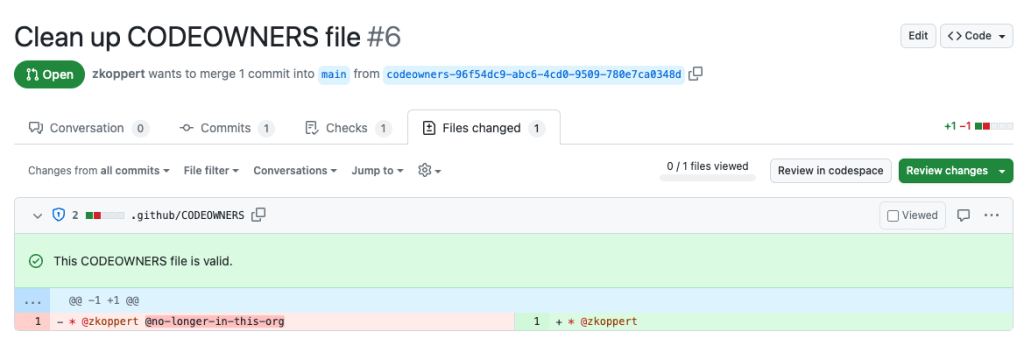

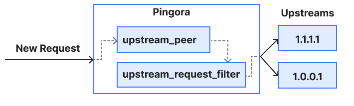

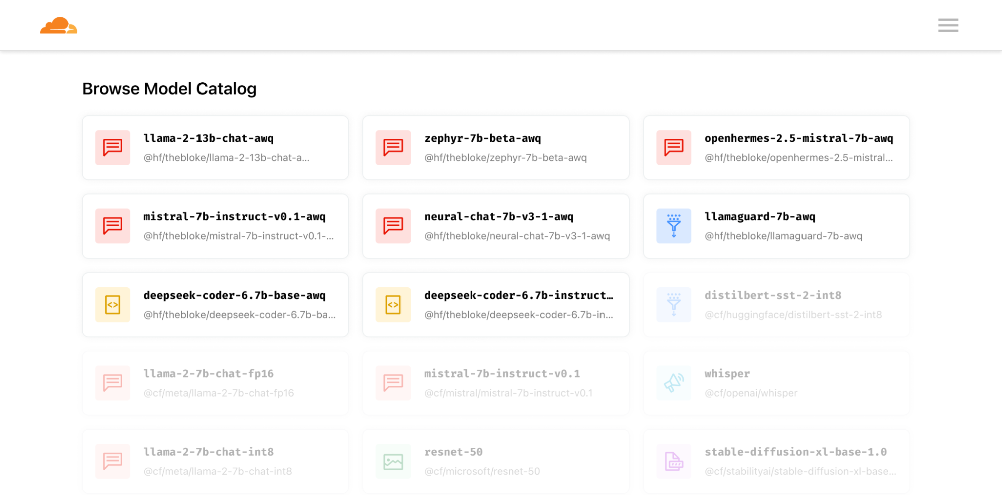


 Anshu Agarwal is a Senior Software Engineer working on AWS OpenSearch at Amazon Web Services. She is passionate about solving problems related to building scalable and highly reliable systems.
 Rishab Nahata is a Software Engineer working on OpenSearch at Amazon Web Services. He is fascinated about solving problems in distributed systems. He is active contributor to OpenSearch.
 Bukhtawar Khan is a Principal Engineer working on Amazon OpenSearch Service. He is interested in distributed and autonomous systems. He is an active contributor to OpenSearch.
 Ranjith Ramachandra is an Engineering Manager working on Amazon OpenSearch Service at Amazon Web Services.
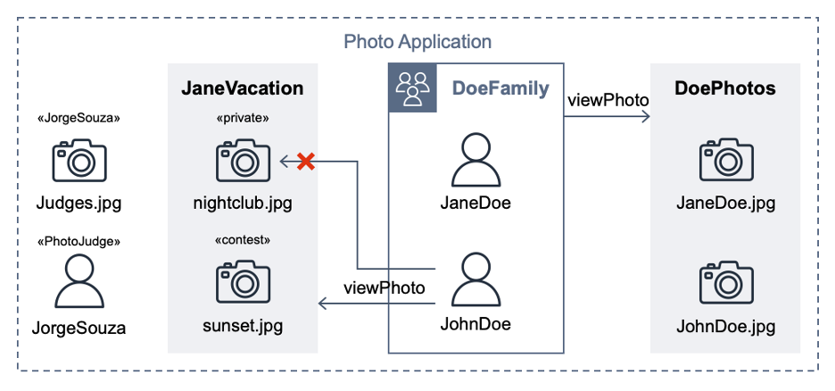
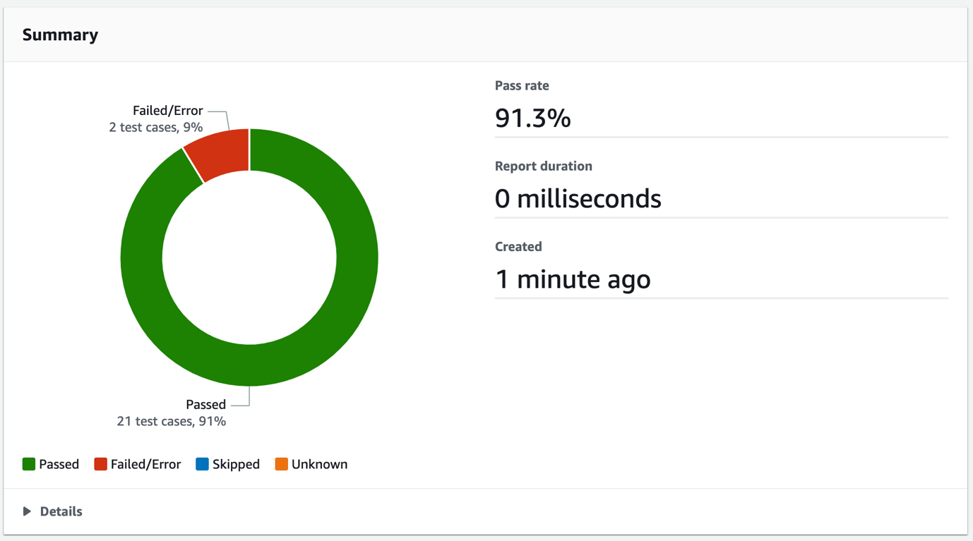
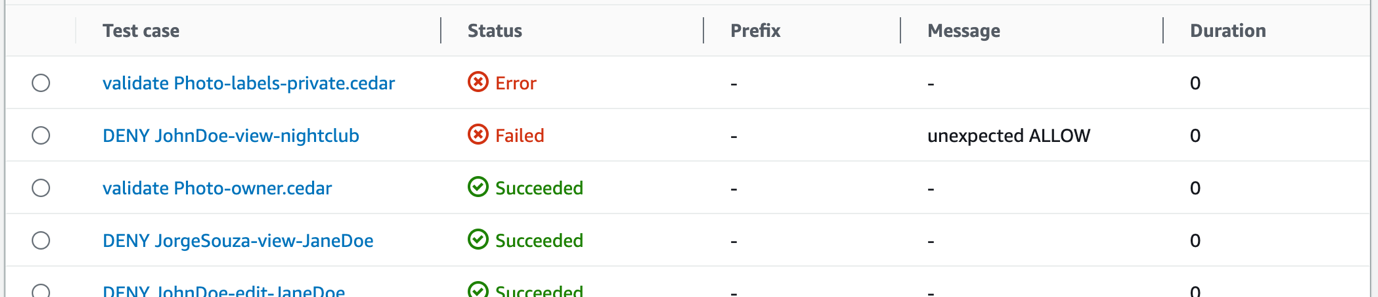
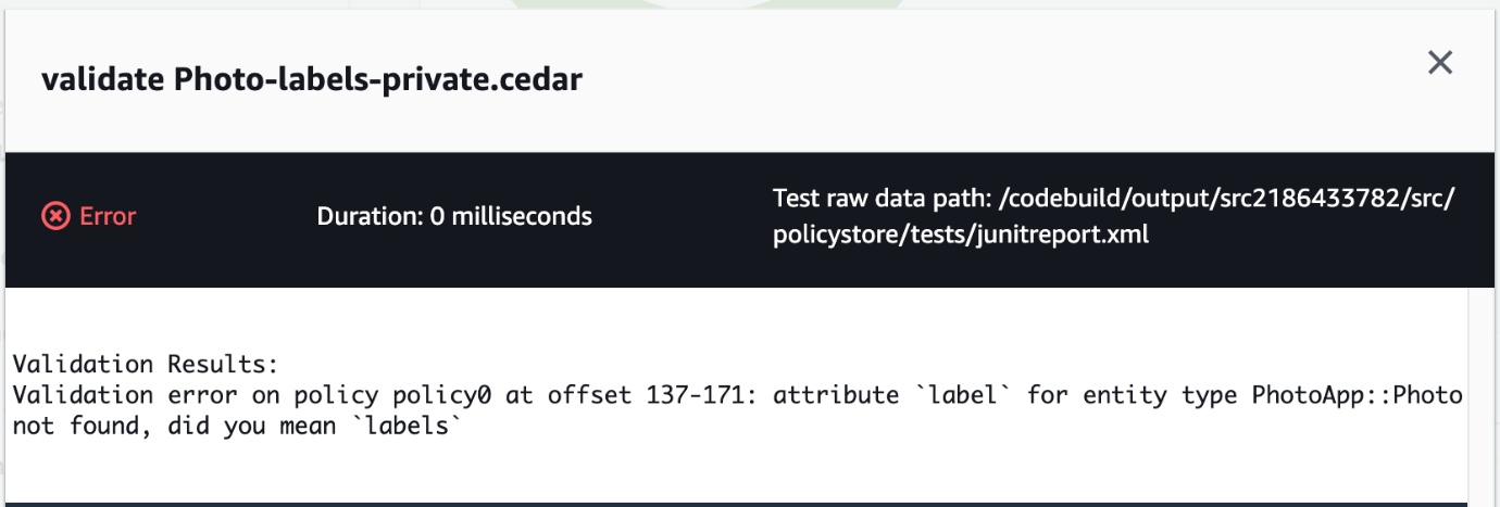

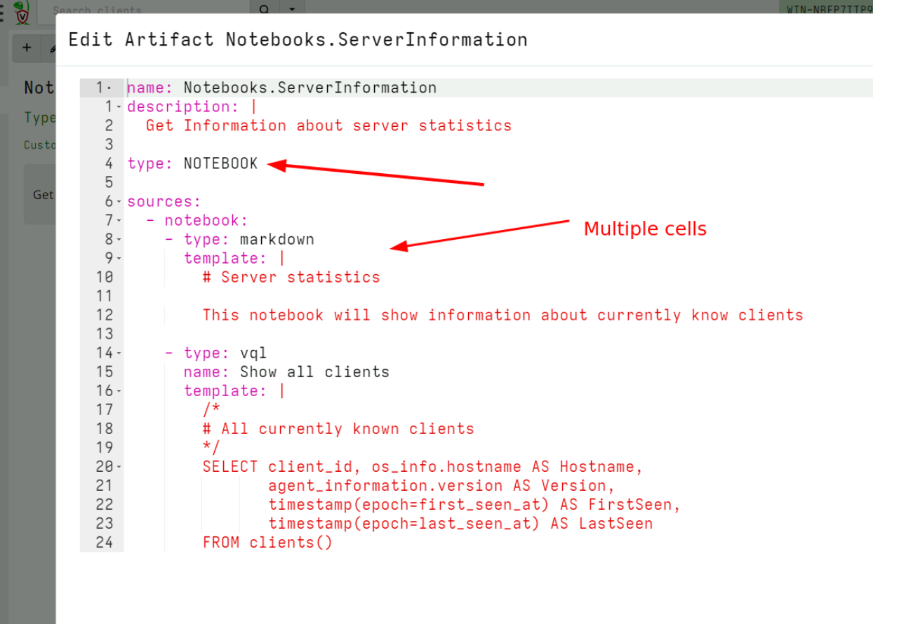
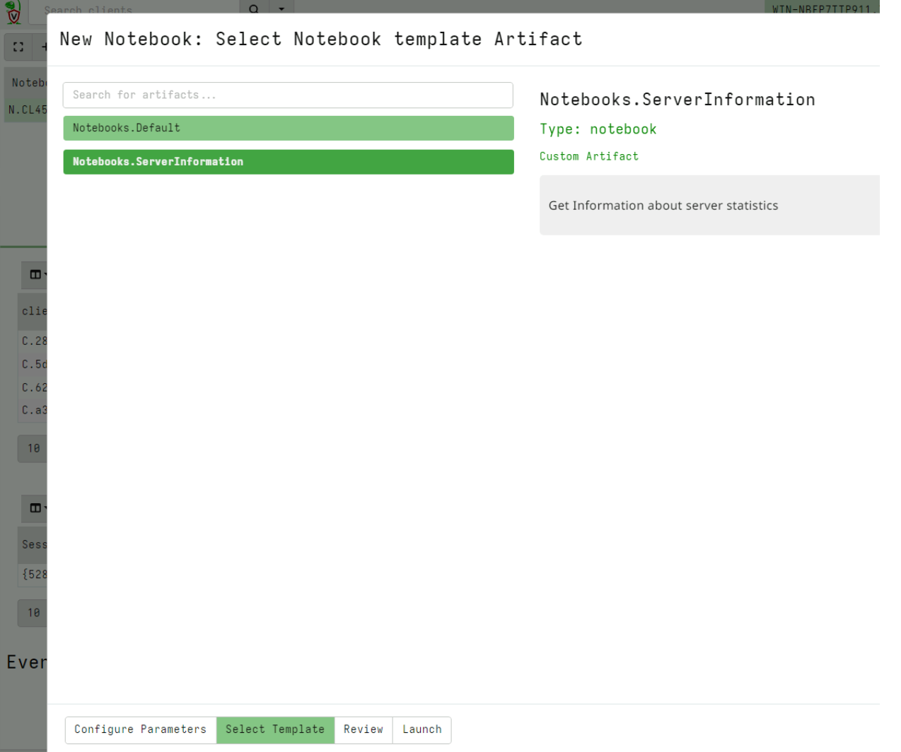
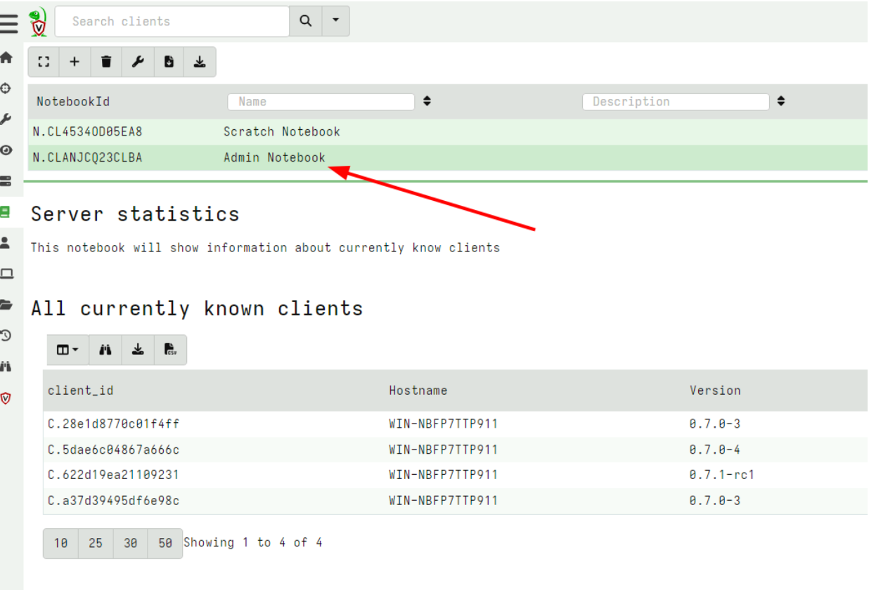
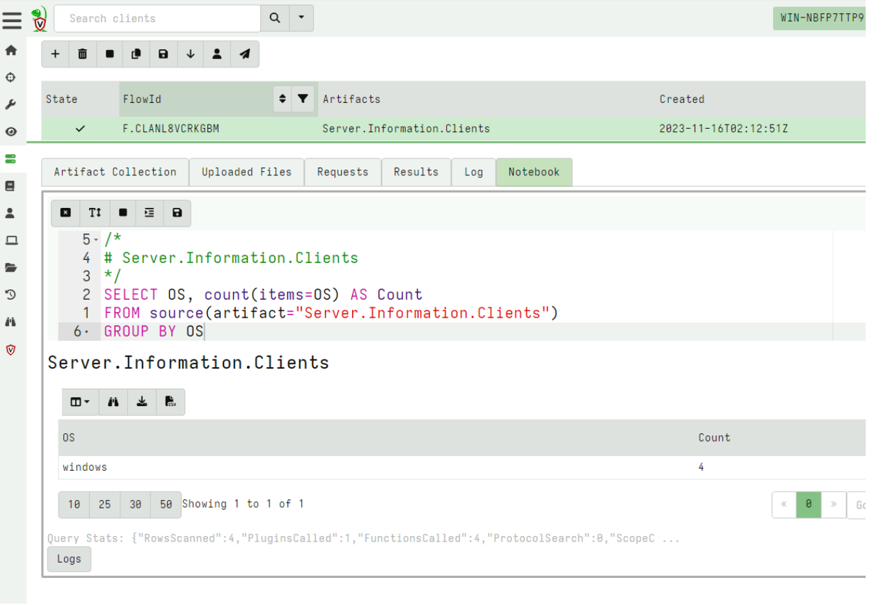
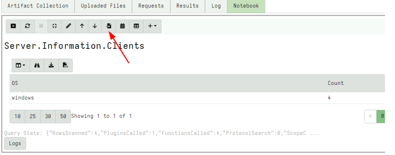
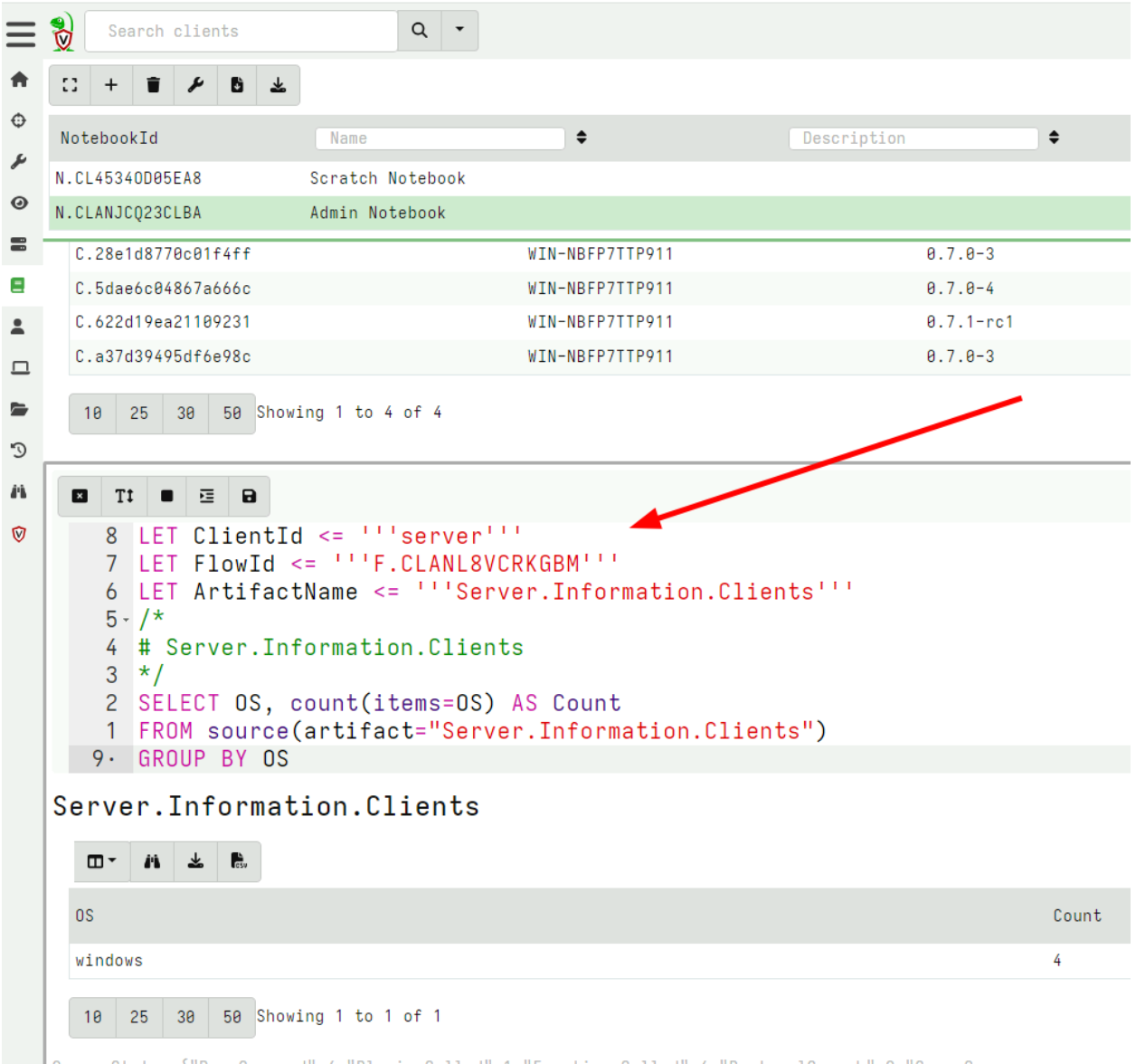
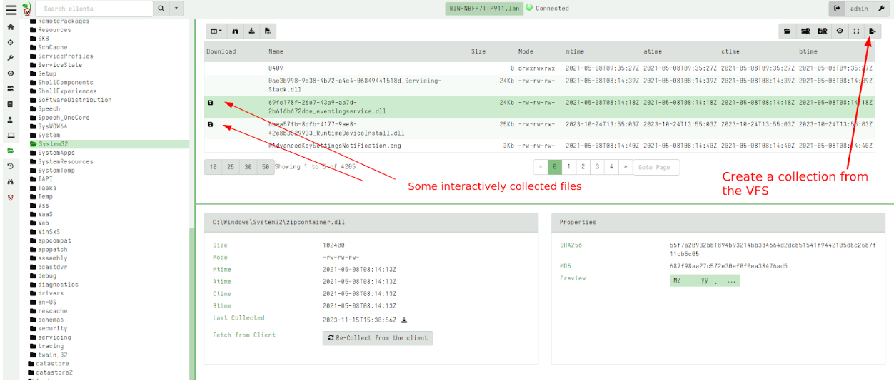
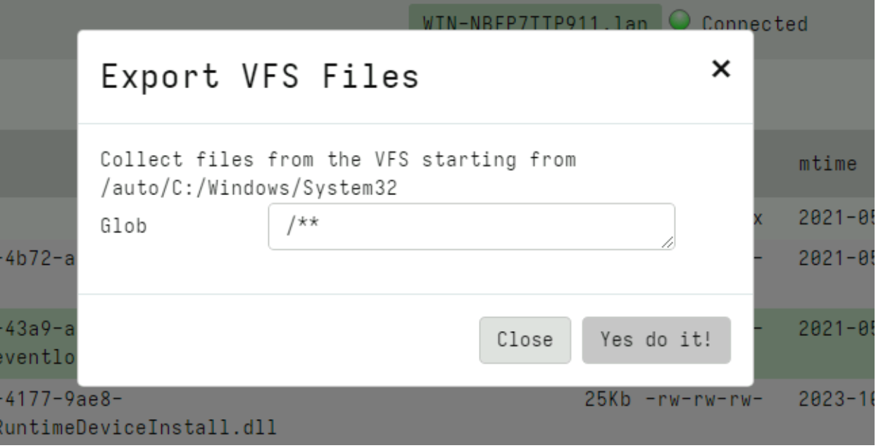
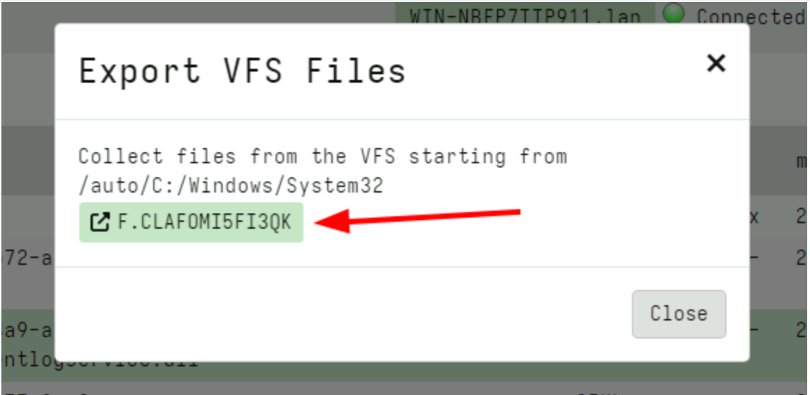
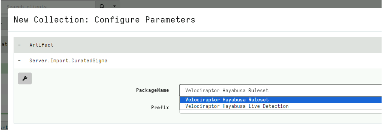
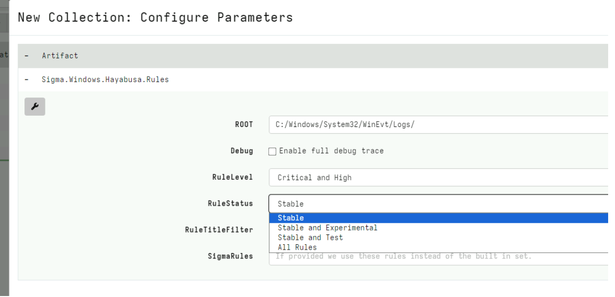
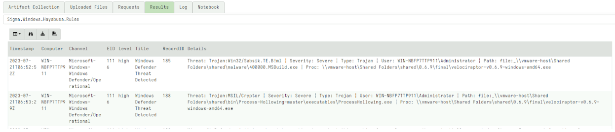
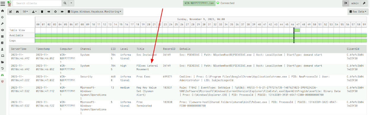
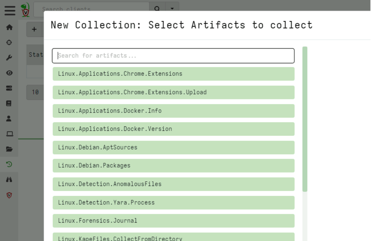
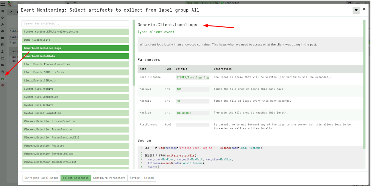
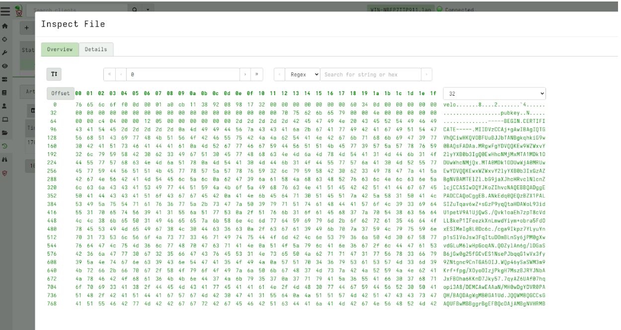
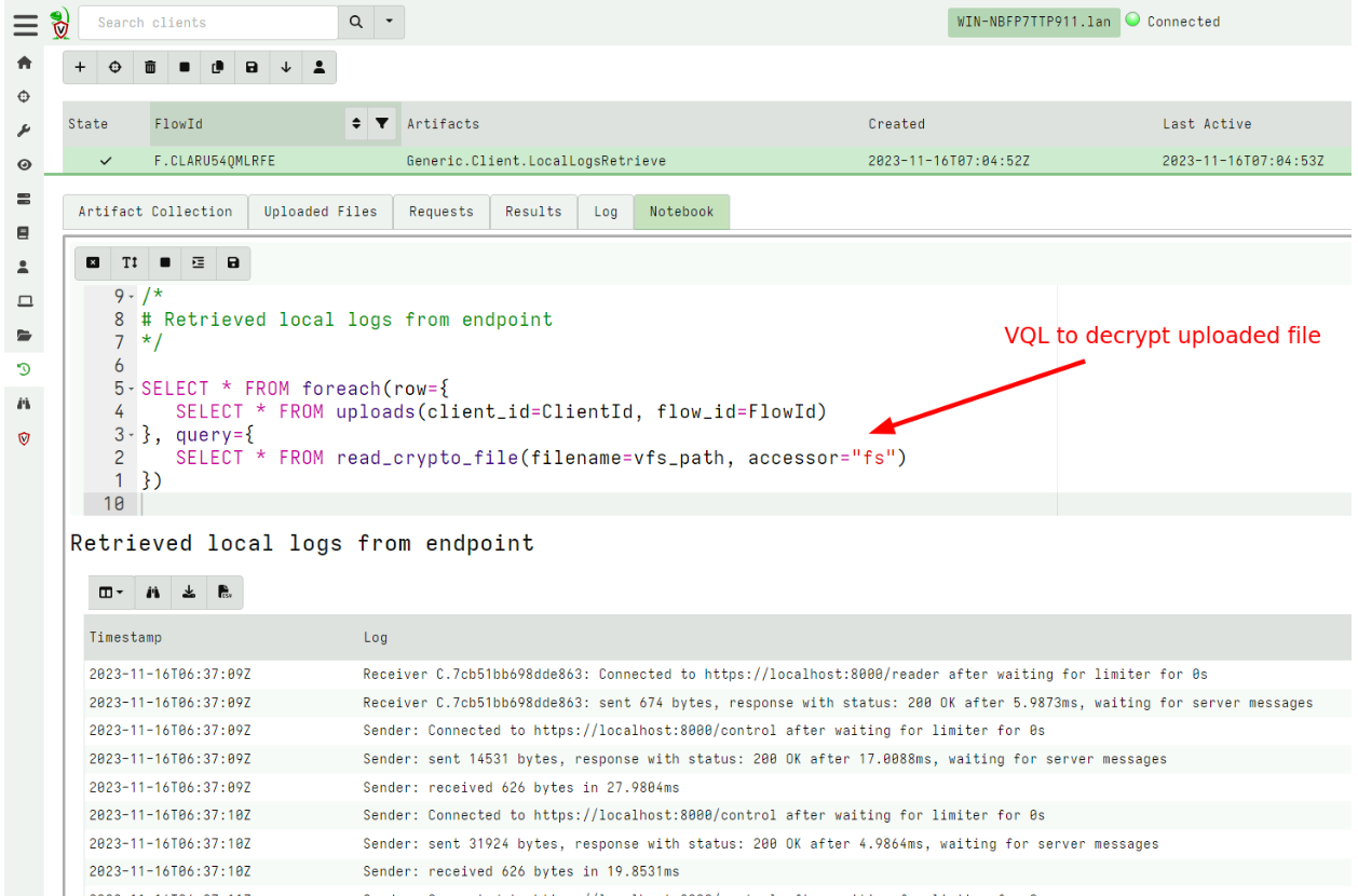


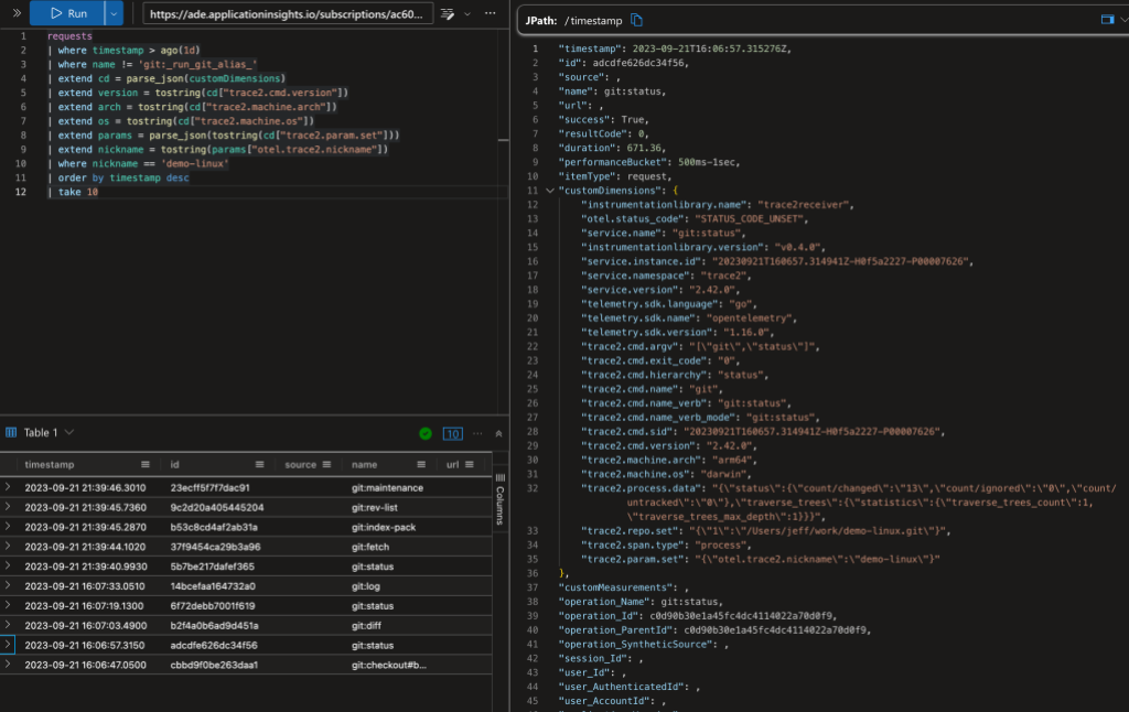
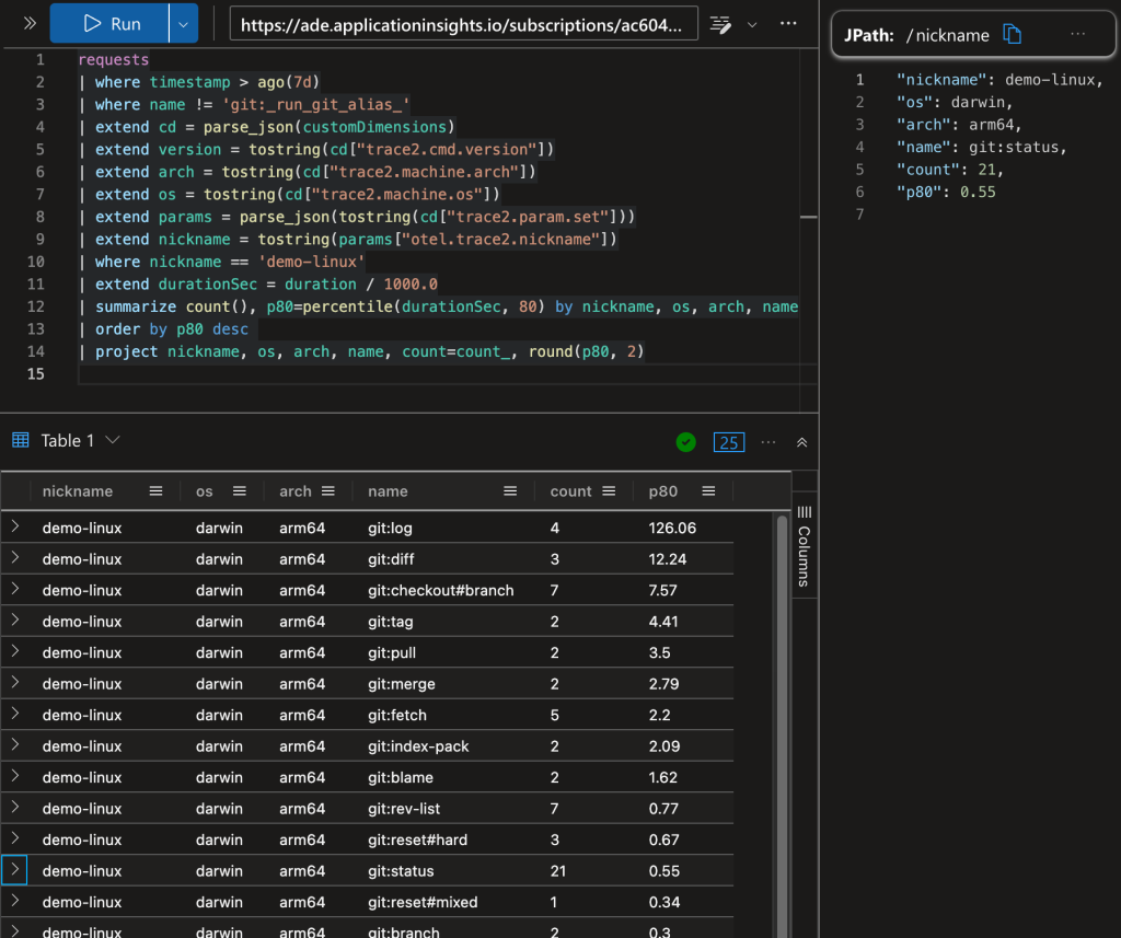

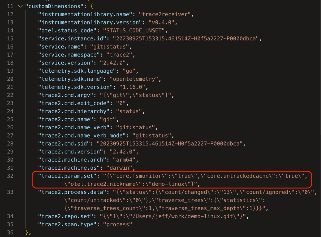
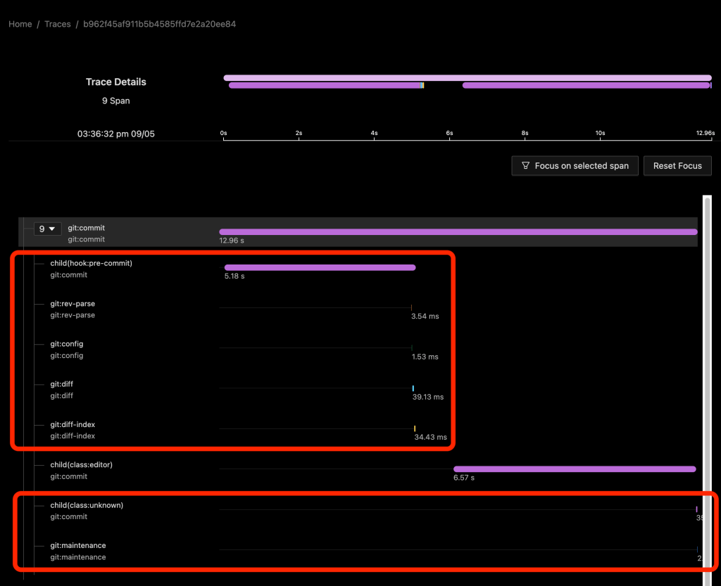


 Since we


