Tag Archives: Intermediate (200)

How to implement single-user secret rotation using Amazon RDS admin credentials

Post Syndicated from Adithya Solai original https://aws.amazon.com/blogs/security/how-to-implement-single-user-secret-rotation-using-amazon-rds-admin-credentials/

You might have security or compliance standards that prevent a database user from changing their own credentials and from having multiple users with identical permissions. AWS Secrets Manager offers two rotation strategies for secrets that contain Amazon Relational Database Service (Amazon RDS) credentials: single-user and alternating-user.

In the preceding scenario, neither single-user rotation nor alternating-user rotation would meet your security or compliance standards. Single-user rotation uses database user credentials in the secret to rotate itself (assuming the user has change-password permissions). Alternating-user rotation uses Amazon RDS admin credentials from another secret to create and update a _clone user credential, which means there are two valid user credentials with identical permissions.

In this post, you will learn how to implement a modified alternating-user solution that uses Amazon RDS admin user credentials to rotate database credentials while not creating an identical _clone user. This modified rotation strategy creates a short lag between when the password in the database changes and when the secret is updated. During this brief lag before the new password is updated, database calls using the old credentials might be denied. Test this in your environment to determine if the lag is within an acceptable range.

Walkthrough

In this walkthrough, you will learn how to implement the modified rotation strategy by modifying the existing alternating-user rotation template. To accomplish this, you need to complete the following:

  • Configure alternating-user rotation on the database credential secret for which you want to implement the modified rotation strategy.
  • Modify your AWS Lambda rotation function template code to implement the modified rotation strategy.
  • Test the modified rotation strategy on your database credential secret and verify that the secret was rotated while also not creating a _clone user.

To configure alternating-user rotation on the database credential secret

  1. Follow this AWS Security Blog post to set up alternating-user rotation on an Amazon RDS instance.
  2. When configuring rotation for the database user secret in the Secrets Manager console, clear the checkbox for Rotate immediately when the secret is stored. The next rotation will begin on your schedule in the Rotation schedule tab. Make sure that no _clone user is created by the default alternating-user rotation code through your database’s user tables.

Figure 1: Clear the checkbox for Rotate immediately when the secret is stored

Figure 1: Clear the checkbox for Rotate immediately when the secret is stored

To modify your Lambda function rotation Lambda template to implement the modified rotation strategy

  1. In the Secrets Manager console, select the Secrets menu from the left pane. Then, select the new database user secret’s name from the Secret name column.

    Figure 2: Select the new database user secret

    Figure 2: Select the new database user secret

  2. Select the Rotation tab on the Secrets page, and then choose the link under Lambda rotation function.

    Figure 3: Select the Lambda rotation function

    Figure 3: Select the Lambda rotation function

  3. From the rotation Lambda menu, Download select Download function code.zip.

    Figure 4: Select Download function code .zip from Download

    Figure 4: Select Download function code .zip from Download

  4. Unzip the .zip file. Open the lambda_function.py file in a code editor and make the following code changes to implement the modified rotation strategy.

    The following code changes show how to modify a rotation function for the MySQL alternating-user rotation code template. You must make similar changes in the CreateSecret and SetSecret steps of the alternating-user rotation code template for your database’s engine type.

    To make the needed changes, remove the lines of code that are in grey italic and add the lines of code that are bold.

    Consider using AWS Lambda function versions to enable reverting your Lambda function to previous iterations in case this modified rotation strategy goes wrong.

    In create_secret()

    The following code suggestion removes the creation of _clone-suffixed usernames.

    Remove:

    -- # Get the alternate username swapping between the original user and the user with _clone appended to it
    -- current_dict['username'] = get_alt_username(current_dict['username'])

    In set_secret()

    The following code suggestions remove the creation of _clone-suffixed usernames and subsequent checks for such usernames in conditional logic.

    Keep:

    # Get username character limit from environment variable
    username_limit = int(os.environ.get('USERNAME_CHARACTER_LIMIT', '16'))

    Remove:

    -- # Get the alternate username swapping between the original user and the user with _clone appended to it
    -- current_dict['username'] = get_alt_username(current_dict['username'])

    Keep:

    # Check that the username is within correct length requirements for version

    Remove:

    -- if current_dict['username'].endswith('_clone') and len(current_dict['username']) > username_limit:

    Add:

    ++ if len(current_dict[‘username’]) > username_limit:

    Keep:

    raise ValueError("Unable to clone user, username length with _clone appended would exceed %s character
    s" % username_limit)
    # Make sure the user from current and pending match

    Remove:

    -- if get_alt_username(current_dict['username']) != pending_dict['username']:

    Add:

    ++ if current_dict['username'] != pending_dict['username']:

    Remove:

    -- def get_alt_username(current_username):
    --   """Gets the alternate username for the current_username passed in
    --
    --   This helper function gets the username for the alternate user based on the passed in current username.
    --
    --   Args:
    --       current_username (client): The current username
    --
    --   Returns:
    --      AlternateUsername: Alternate username
    --
    --   Raises:
    --      ValueError: If the new username length would exceed the maximum allowed
    --
    --   """
    --   clone_suffix = "_clone"
    --   if current_username.endswith(clone_suffix):
    --       return current_username[:(len(clone_suffix) * -1)]
    --   else:
    --       return current_username + clone_suffix
    --

    The following code suggestions remove the logic of creating a new _clone user within the database, and rotates the existing user’s password.

    Keep:

    with conn.cursor() as cur:

    Remove:

    --   cur.execute("SELECT User FROM mysql.user WHERE User = %s", pending_dict['username'])
    --   # Create the user if it does not exist
    --   if cur.rowcount == 0:
    --      cur.execute("CREATE USER %s IDENTIFIED BY %s", (pending_dict['username'], pending_dict['password']))
    -- 
    --   # Copy grants to the new user
    --   cur.execute("SHOW GRANTS FOR %s", current_dict['username'])
    --   for row in cur.fetchall():
    --       grant = row[0].split(' TO ')
    --       new_grant_escaped = grant[0].replace('%', '%%')  # % is a special character in Python format strings.
    --       cur.execute(new_grant_escaped + " TO %s", (pending_dict['username'],))

    Keep:

        # Get the version of MySQL
        cur.execute("SELECT VERSION()")
        ver = cur.fetchone()[0]

    Remove:

    --   # Copy TLS options to the new user
    --   escaped_encryption_statement = get_escaped_encryption_statement(ver)
    --   cur.execute("SELECT ssl_type, ssl_cipher, x509_issuer, x509_subject FROM mysql.user WHERE User = %s", current_dict['username'])
    --   tls_options = cur.fetchone()
    --   ssl_type = tls_options[0]
    --   if not ssl_type:
    --       cur.execute(escaped_encryption_statement + " NONE", pending_dict['username'])
    --   elif ssl_type == "ANY":
    --       cur.execute(escaped_encryption_statement + " SSL", pending_dict['username'])
    --   elif ssl_type == "X509":
    --       cur.execute(escaped_encryption_statement + " X509", pending_dict['username'])
    --   else:
    --       cur.execute(escaped_encryption_statement + " CIPHER %s AND ISSUER %s AND SUBJECT %s", (pending_dict['username'], tls_options[1], tls_options[2], tls_options[3]))

    Keep:

        # Set the password for the user and commit
        password_option = get_password_option(ver)
        cur.execute("SET PASSWORD FOR %s = " + password_option, (pending_dict['username'], pending_dict['password']))
        conn.commit()
        logger.info("setSecret: Successfully set password for %s in MySQL DB for secret arn %s." % (pending_dict['username'], arn))

  5. Re-zip the folder with the local code changes. From the rotation Lambda menu, under the Code tab, choose Upload from and select .zip file. Upload the new .zip file.

    Figure 5: Use Upload from to upload the new .zip file as the Code source

    Figure 5: Use Upload from to upload the new .zip file as the Code source

To test the modified rotation strategy

  1. During the next scheduled rotation for the new database user secret, the modified rotation code will run. To test this immediately, select the Rotation tab within the Secrets menu and choose Rotate secret immediately in the Rotation configuration section.

    Figure 6: Choose Rotate secret immediately to test the new rotation strategy

    Figure 6: Choose Rotate secret immediately to test the new rotation strategy

  2. To verify that the modified rotation strategy worked, verify the sign-in details in both the secret and the database itself.
    1. To verify the Secrets Manager secret, select the Secrets menu in the Secrets Manager console and choose Retrieve secret value under the Overview tab. Verify that the username doesn’t have a _clone suffix and that there is a new password. Alternatively, make a get-secret-value call on the secret through the AWS Command Line Interface (AWS CLI) and verify the username and password details.

      Figure 7: Use the secret details page for the database user secret to verify that the value of the username key is unchanged

      Figure 7: Use the secret details page for the database user secret to verify that the value of the username key is unchanged

    2. To verify the sign-in details in the database, sign in to the database with admin credentials. Run the following database command to verify that no users with a _clone suffix exist: SELECT * FROM mysql.user;. Make sure to use the commands appropriate for your database engine type.
    3. Also, verify that the new sign-in credentials in the secret work by signing in to the database with the credentials.

Clean up the resources

  • Follow the Clean up the resources section from the AWS Security Blog post used at the start of this walkthrough.

Conclusion

In this post, you’ve learned how to configure rotation of Amazon RDS database users using a modified alternating-users rotation strategy to help meet more specific security and compliance standards. The modified strategy ensures that database users don’t rotate themselves and that there are no duplicate users created in the database.

You can start implementing this modified rotation strategy through the AWS Secrets Manager console and Amazon RDS console. To learn more about Secrets Manager, see the Secrets Manager documentation.

If you have feedback about this post, submit comments in the Comments section below. If you have questions about this post, start a new thread on AWS Secrets Manager re:Post or contact AWS Support.

Want more AWS Security news? Follow us on X.

Adithya Solai

Adithya Solai

Adithya is a software development engineer working on core backend features for AWS Secrets Manager. He graduated from the University of Maryland, College Park, with a BS in computer science. He is passionate about social work in education. He enjoys reading, chess, and hip-hop and R&B music.

Integrating AWS Verified Access with Jamf as a device trust provider

Post Syndicated from Mayank Gupta original https://aws.amazon.com/blogs/security/integrating-aws-verified-access-with-jamf-as-a-device-trust-provider/

In this post, we discuss how to architect Zero Trust based remote connectivity to your applications hosted within Amazon Web Services (AWS). Specifically, we show you how to integrate AWS Verified Access with Jamf as a device trust provider. This post is an extension of our previous post explaining how to integrate AWS Verified Access with CrowdStrike. In this post, we also look at how to troubleshoot Verified Access policies and integration issues for when a user with valid access receives access denied or unauthorized error messages.

Verified Access is a networking service that is built on Zero Trust principles and provides secured access to corporate applications without needing a virtual private network (VPN). This enables your corporate users to be able to access their applications from anywhere with a complaint device. Verified Access reduces IT operations overhead because it is built on an open environment and integrates with your existing trust providers and lets you use your existing implementations.

Verified Access lets you centrally define access policies for your applications with additional context beyond only IP address, using claims from user identity and user device coming from the trust providers. Using these access policies, Verified Access evaluates each access request at scale in real time and records each access request centrally, making it easier and quicker for you to respond to security incidents or audit requests.

Jamf is an Apple mobile device management (MDM) software and security provider. Organizations can use Jamf to manage their corporate devices and maintain security posture. Jamf’s Zero Trust product—Jamf Trust—monitors device security posture and reports it back to the administrators on the Jamf Protect console. It monitors the device’s OS settings, patch level, and device settings against an organization’s defined policy and calculates device posture from secure to high risk.

Verified Access integrates with third-party device management providers such as Jamf to gather additional security claims from the device in addition to user identity to either allow or deny access.

Solution overview

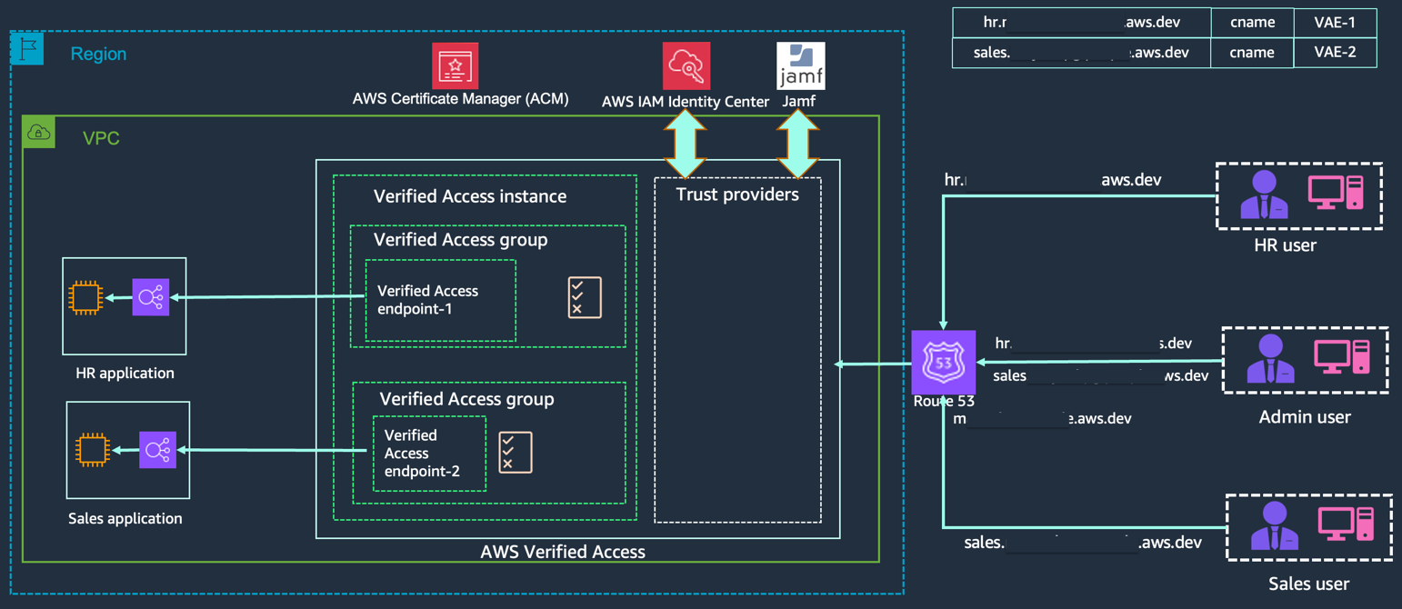
In this example, you will set up remote access to a sales application and an HR application. Through the solution, you want to make sure only users from the sales group can access the sales application, and only users from the HR group are able to access the HR application.

You will onboard the applications to Verified Access, and access policies will be defined based on the security requirements using Cedar as the policy language. After you have onboarded the applications and have defined the access policies, engineers and users will be able to access the application from anywhere using the Verified Access endpoint without needing a VPN.

You will also use the claims coming from the device in the access policies to make sure that device is managed by Jamf and is secure—for example, that the device is at the right patch level or there are no security vulnerabilities—before granting user access to the respective application.

Figure 1: High-level solution architecture

Figure 1: High-level solution architecture

Prerequisites

To integrate Verified Access with Jamf device trust provider, you need to have the following prerequisites.

Verified Access:

  1. Enable AWS IAM Identity Center for your entire AWS Organization. If you don’t have it enabled, follow the steps to enable AWS IAM Identity Center
  2. Have users created and mapped to respective groups under AWS IAM Identity Center
  3. Apple device (EC2 Mac for this demo)
  4. Subscription with Jamf Pro and Jamf Security (RADAR)
  5. Jamf tenant ID

Jamf:

  1. Managed devices with Jamf Pro
  2. Volume purchasing for app deployment
  3. MacOS 12 or later

Walkthrough

For this demo, you will use Amazon Elastic Compute Cloud (Amazon EC2) Mac instances, which will be enrolled and managed by Jamf. Because EC2 Mac instances don’t come with MDM capabilities out of the box, you can use the following steps to enroll an EC2 Mac instance with Jamf.

Enroll EC2 Mac instance with Jamf

To start, you need to create some credentials and store them in AWS Secrets Manager. These credentials are Jamf endpoint, Jamf user and password with enrollment privileges, and the EC2 Mac instance local admin and the password. We have used AWS Secrets Manager for this demo, but if desired, you could use Parameter Store, a capability of AWS Systems Manager. You can find AWS CloudFormation and Terraform templates for both Secrets Manager and Systems Manager at our sample code on GitHub.

The CloudFormation template will create:

  1. jamfServerDomain – This is your organization’s Jamf URL, the endpoint for your device to get the enrollment from.
  2. jamfEnrollmentUser – This is the authorized user within Jamf with device enrollment permissions.
  3. jamfEnrollmemtPassword – This is the password for the enrollment user provided in number 2.
  4. localAdmin – This is the admin user on your EC2 Mac instance, with the permissions to install required profiles and apply changes.
  5. localAdminPassword – This is the password for the admin user on your EC2 Mac instance provided in number 4.

The CloudFormation template also creates a Secrets Manager secret, an AWS Identity and Access Management (IAM) policy, a role, and an instance profile.

To allocate a Dedicated Host and launch an EC2 Mac instance

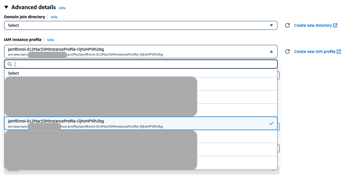
After you complete deploying the CloudFormation template, allocate an Amazon EC2 Dedicated Host for Mac and launch an EC2 Mac instance on the host. On the Launch an instance screen, after providing the basic details, expand the Advanced details section and select the IAM instance profile that was created as part of CloudFormation deployment.

Figure 2: Advanced details pane showing the selected IAM instance profile

Figure 2: Advanced details pane showing the selected IAM instance profile

To configure the instance:

  1. Connect to your EC2 Mac instance using Secure Shell (SSH).

    Figure 3: The steps for connecting to the instance using SSH client

    Figure 3: The steps for connecting to the instance using SSH client

  2. Enable screen sharing and set the admin password to the one you used when creating credentials. Use the following command:
    sudo /usr/bin/dscl . -passwd /Users/ec2-user 'l0c4l3x4mplep455w0rd' ; sudo launchctl enable system/com.apple.screensharing ; sudo launchctl load -w /System/Library/LaunchDaemons/com.apple.screensharing.plist

  3. After screen sharing is enabled, connect to the EC2 Mac instance using VNC Viewer or a similar tool and enable automatic login from System Settings – > Users & Groups
  4. Place the AppleScript provided on the GitHub in /Users/Shared:
    1. You can either download the script to your local machine and then copy it over or download the script directly to the EC2 Mac instance.
    2. If you are using VNC Viewer to connect to the instance, you should be able to drag and drop the file from your local machine to the EC2 Mac instance.
  5. Edit and update the AppleScript with the secret ID from Secrets Manager for the MMSecret variable:
    1. MMSecret is the secret from the Secrets Manager that was created as part of the CloudFormation template deployment. Copy the secret Amazon Resource Name (ARN) from the Secrets Manager console or use the AWS Command Line Interface (AWS CLI) to get the ARN and update it in the AppleScript.
  6. Run the AppleScript using the following command and allow access to Accessibility, App Management, and Disk Access permissions for the script. While the script is running, the screen might flash a few times.
    osascript /Users/Shared/enroll-ec2-mac.scpt --setup

  7. After you see the Successful message, choose OK and restart the instance. After the instance has restarted, sign in to the instance and the enrollment will proceed.

The enrollment will take a few minutes and your EC2 Mac instance will receive the profiles and policies from the Jamf instance as configured by your administrator.

Jamf end setup for Verified Access

In this section, you will be working on your Jamf security portal, RADAR, to integrate Verified Access with Jamf, and then onboard your applications to Verified Access and define access policies. You begin this walkthrough by enabling Verified Access on Jamf first.

Jamf Protect and Jamf Trust are the components that collect device claims and share them with Verified Access. The following section illustrates how to make Jamf ready to send claims over to Verified Access. This section needs to be completed on Jamf Security and Jamf Pro Portals. Jamf UI can differ depending on the Jamf Pro version used.

To enable Verified Access profile and deploy Jamf Trust and Verified Access browser extensions

  1. Create an AWS Verified Access activation profile:
    1. Go to Jamf RADAR portal -> Devices -> Activation profiles.
    2. Choose Create profile. If presented with an option, choose Jamf Trust.
    3. Select Device identity from the options available and choose Next.
    4. Select Without identity provider and Assign random identifier and choose Next.
    5. Leave the following sections as they are and continue to choose Next until you reach the review screen.
    6. Choose Save and Create.
  2. Download the manifest files:
    1. Select the profile created in Step 1.
    2. Select your UEM (Jamf Pro in our case).
    3. Select your OS (macOS in our case).
    4. Download Configuration profiles and Browser manifests.
  3. Deploy Jamf Trust using Jamf Pro:
    1. For Jamf Trust, go to the App Store apps in your Jamf Pro instance.
    2. Search for and add Jamf Trust for deployment.
    3. For deployment method, select Install Automatically.
    4. Define scope for target computers and save.
  4. Deploy configuration profiles using Jamf Pro:
    1. Navigate to Configuration Profiles.
    2. Choose Upload and select the configuration file downloaded from the RADAR portal and upload it.
    3. In the General payload configuration tab, select basic settings and distribution method.
    4. Define scope for target computers and choose Save.
  5. Deploy browser extensions using Jamf Pro:
    1. Navigate to Settings -> computer management, choose Packages, and choose New.
    2. Use the general pane to define basic settings.
    3. Select Choose File and select the Verified Access PKG file downloaded from the RADAR portal to upload and choose Save.
    4. Navigate to Policies under Computers and choose New to create a new policy and use the general pane to define basic settings.
    5. Select Packages and choose Configure.
    6. Choose Add for the package you want to install and choose Install under Actions.
    7. Define scope for target computers and choose Save.
  6. Create and deploy Verified Access browser extensions (Google Chrome):
    1. In Jamf Pro, at the top of the sidebar, select Computers. In the sidebar, select Configuration Profiles and choose New.
    2. In General, use the default basic settings, including the level at which to apply the profile and the distribution method.
    3. Select the Application & Custom Settings, and then choose External Applications and choose Add.
    4. In the Source section, from the Choose source pop-up menu, choose Jamf Repository.
    5. In the Application Domain section, choose com.google.chrome. Select the default options for version and variant choices.
    6. Choose Add/Remove properties and deselect the Cloud Management Enrollment Token and, in the Custom Property field, enter ExtensionInstallForcelist, then choose Add and choose Apply.
    7. In the ExtensionInstallForcelist pop-up menu, select Array. For item 1, select String from the pop-up menu, and enter the following ID for the Google Chrome browser extension: aepkkaojepmbeifpjmonopnjcimcjcbd.
    8. Select the Scope tab and configure the scope of the profile and choose Save.
  7. Create and deploy Verified Access browser extensions (Firefox):
    1. In Jamf Pro, at the top of the sidebar, select Computers.
    2. Select Configuration Profiles in the sidebar and choose New.
    3. In General, use the default basic settings, including the level at which to apply the profile and the distribution method.
    4. Select the Application & Custom Settings payload, choose External Applications > Upload, and choose Add.
    5. In the Preference Domain field, enter org.mozilla.firefox.
    6. Use the following code to create the desired policies for browser extension behavior. Key-value pairs in the following sample PLIST can be modified to match desired policy options.
      <dict>
      <key>EnterprisePoliciesEnabled</key>
      <true/>
      <key>ExtensionSettings</key>
      <dict>
      <key>verified-access@amazonaws</key>
      <dict>
      <key>install_url</key>
      <string>https://addons.mozilla.org/firefox/downloads/latest/aws-verified-access/latest.xpi</string>
      <key>installation_mode</key>
      <string>normal_installed</string>
      </dict>
      </dict>
      </dict>

    7. Select the Scope tab and configure the scope of the profile and choose Save.

To obtain your Jamf tenant ID for integrating with Verified Access:

  1. Navigate to your Jamf Security console.
  2. Navigate to Integrations and choose Access providers.
  3. Choose Verified Access and choose the connection name.
  4. Your Jamf Customer ID is your tenant ID you’ll use during the setup of integration.

    Figure 4: Jamf tenant ID

    Figure 4: Jamf tenant ID

To review your managed device posture within the Jamf security console:

  1. Navigate to your Jamf Security console.
  2. Navigate to Reports -> Security -> Device view to review current device posture of your managed devices.

    Figure 5: Device posture within Jamf

    Figure 5: Device posture within Jamf

Verified Access setup

There are four steps to onboard your applications to Verified Access:

  1. Onboard Verified Access trust providers.
  2. Create a Verified Access instance.
  3. Create one or more Verified Access groups.
  4. Onboard your application and create Verified Access endpoints.

The following steps explain in detail how to onboard your applications to Verified Access.

Step 1: Onboard Verified Access trust providers

Create a user trust provider

  1. Open the Amazon VPC console. In the navigation pane, choose Verified Access trust providers, and then Create Verified Access trust provider.
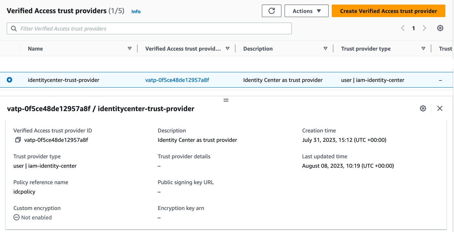
  2. Provide a Name and Description. The screenshot shows identitycenter-trust-provider as the name and Identity Center as trust provider as the description.
  3. Provide a Policy Reference name that you will use later while defining policies. This screenshot shows idcpolicy as the policy reference name.
  4. Select User Trust Provider.
  5. Select IAM Identity Center.
  6. Provide additional tags.
  7. Choose Create Verified Access trust provider.

Figure 6: This screenshot shows that user identity trust providers have been created

Figure 6: This screenshot shows that user identity trust providers have been created

Create a device trust provider

  1. Open the Amazon VPC console. In the navigation pane, choose Verified Access trust providers, and then Create Verified Access trust provider.
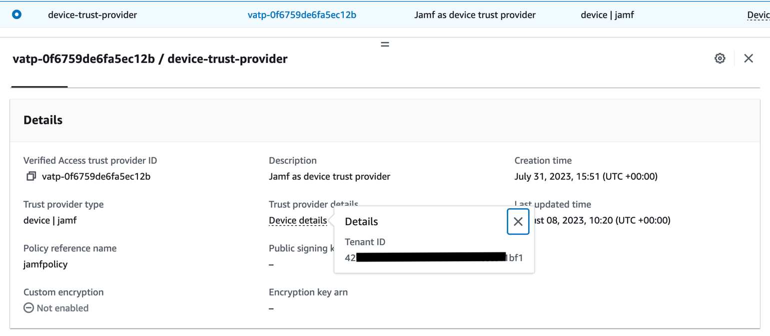
  2. Provide a Name and Description. The screenshot shows device-trust-provider as the name and Jamf as device trust provider as the description.
  3. Provide a Policy Reference name that you will use later while defining policies. The screenshot shows jamfpolicy as the policy reference name.
  4. Select Device trust provider.
  5. In Device details, provide the Jamf tenant ID that you obtained from the Jamf Security console.
  6. Provide additional tags.
  7. Choose Create Verified Access trust provider.

Figure 7: This screenshot shows the device trust provider has been created

Figure 7: This screenshot shows the device trust provider has been created

Step 2: Create a Verified Access instance

  1. Open the Amazon VPC console. In the navigation pane, choose Verified Access instances, and then Create Verified Access instance. Provide a Name and Description.
  2. From the dropdown list, select one of the trust providers you created in Step 1. You can only select one trust provider at the time of instance creation.
  3. Provide additional tags and choose Create Verified Access instance.
  4. After the instance is created, select the instance and choose Actions.
  5. Choose Attach Verified Access trust provider.
  6. Select the other trust provider from the dropdown list and choose Attach Verified Access trust provider.

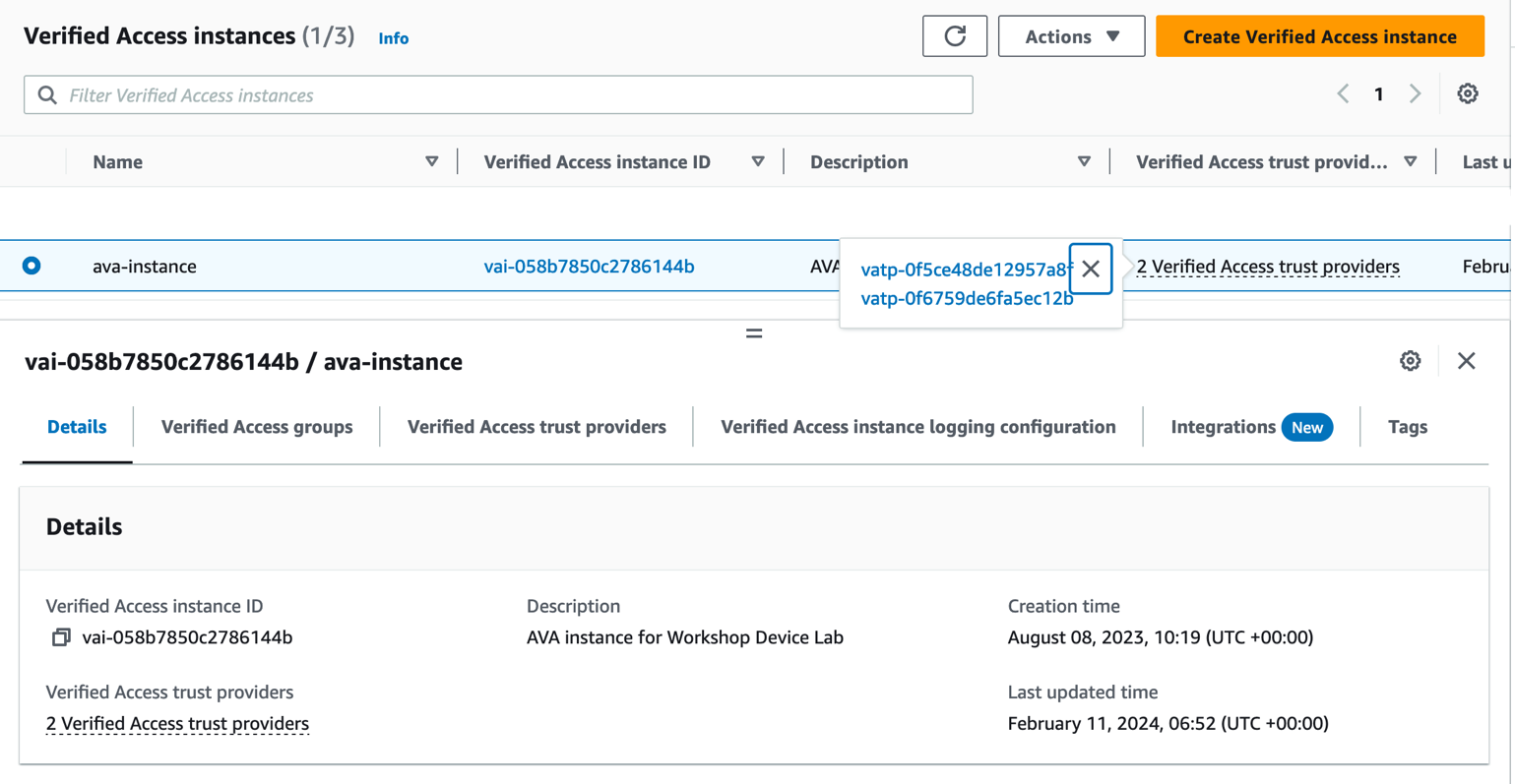
Figure 8: The Verified Access instance has been created with both trust providers attached

Figure 8: The Verified Access instance has been created with both trust providers attached

Step 3: Create Verified Access groups

  1. Open the Amazon VPC console. In the navigation pane, choose Verified Access groups, and then Create Verified Access group.
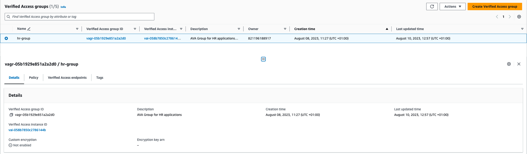
  2. Provide a Name and Description. The screenshot shows hr-group for the name and AVA Group for HR application as the description.
  3. Select the Verified Access instance from the dropdown list that you created in Step 2.
  4. Leave policy empty for now. You will define the access policy later.
  5. Choose Create Verified Access group.

You need to repeat the preceding steps for HR applications, creating two groups, one for each application.

Figure 9: HR group successfully created

Figure 9: HR group successfully created

Step 4: Create Verified Access endpoints

Before proceeding with the endpoint creation, make sure you have your application deployed with an internal Application Load Balancer, and you have requested an ACM certificate for your public domain that your users will use to access the application.

  1. Open the Amazon VPC console. In the navigation pane, choose Verified Access endpoints and then Create Verified Access endpoint.
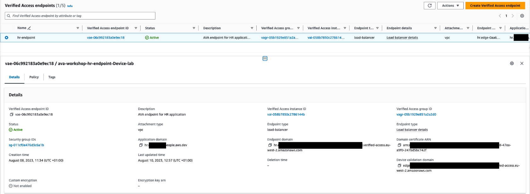
  2. Provide a Name and Description. The example has hr-endpoint for name and AVA endpoint for HR application as the description.
  3. Select the HR Group that you created in Step 3 from the dropdown list.
  4. Under Application Domain, provide the public DNS name for your application and then select the public TLS certificate created and stored to the ACM. For example: hr.xxxxx.people.aws.dev.
    1. Verified Access supports wildcard certificates, which means that you can use a wildcard certificate for all your endpoints, but it doesn’t support wildcard endpoints, which means you cannot have a single endpoint mapping to multiple hostnames.
  5. For attachment type, select VPC.
  6. Select the Security group to be used for the endpoint. Traffic from the endpoint that enters your load balancer is associated with this security group.
  7. For Endpoint type, choose Load balancer. Select the HTTP, port 80, load balancer ARN, and subnet.
  8. Choose Create Verified Access Endpoint.

Repeat the same steps to create an endpoint for the HR application.

It can take a few minutes for the endpoint to become active. Your endpoints are active when you see Active in the Status field.

Figure 10: The HR application endpoint has been created

Figure 10: The HR application endpoint has been created

Create Verified Access policies using trust data from user and device trust providers

Before you make the application available on your public domain for your users, define the access policies for your applications.

Verified Access policies are written in Cedar, an AWS policy language. Review the Verified Access policies documentation for details on policy syntax. The context that is available to use in policies varies based on the trust provider. You can review Trust data from trust providers to learn more about the available trust data for supported trust providers.

To Create or modify group level policy:

You now need to define an access policy for your applications at the group level.

  1. In the Amazon VPC console, select Verified Access groups.
  2. Select one of the groups you created earlier for your application.
  3. From Actions, choose Modify Verified Access Group Policy.
  4. In the policy document, provide the following policy:
    permit(principal,action,resource)
    when {
        context.idcpolicy.groups has "d6e20264-4081-7021-48df-def4276a19fe" &&
        context.idcpolicy.user.email.address like "*@example.com" &&
        context has "jamfpolicy" &&
        context.jamfpolicy has "risk" &&
        ["LOW","SECURE"].contains(context.jamfpolicy.risk)
    };

  5. Choose Modify Verified Access group policy.

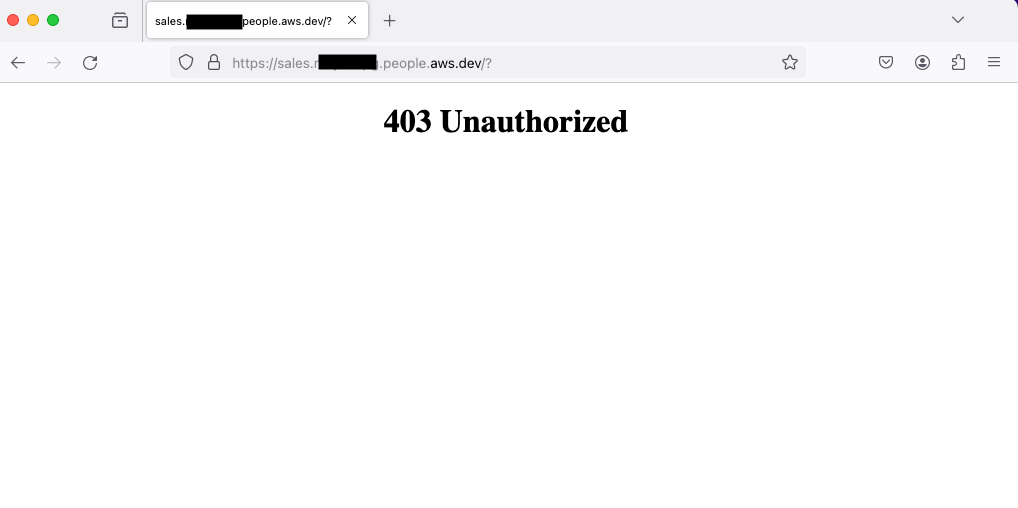
The policy checks for claims received from the user trust provider (IAM Identity Center) and the device trust provider (Jamf). Based on these claims, it makes a decision whether the user is authorized to access the application. In the preceding policy, you check whether the user who is trying to access this application belongs to a certain group and has an email ending with example.com in IAM Identity Center by referencing to the idcpolicy context, which you defined while creating the user trust provider. Similarly, you use the jamfpolicy to reference the context coming from Jamf to validate whether the device used for accessing this application is secure or not. If access criteria aren’t matched, the user will receive a 403 Unauthorized error.

You need to repeat the preceding steps for the other group, defining the access policy with relevant group ID and claims for the application.

Amazon Route 53 configuration

After you complete your Verified Access setup and have defined your access policies, you will make your application public for your users to be able to access from anywhere, without a VPN and in a secure manner. For that, you will update your Amazon Route 53 records with the endpoints you created in Step 4: Create Verified Access endpoints.

  1. In the Amazon VPC console, select Verified Access endpoints.
  2. Select one of the endpoints you created earlier for your application.
  3. From the Details section, make a note of the Endpoint domain. Repeat these two steps for the other endpoint as well and make a note of the endpoint domain.
  4. Go to the Amazon Route53 console and in your hosted zone, choose Click Record.
  5. Provide a Record name. This is the subdomain your users will use to access the application.
  6. For Record type select CNAME.
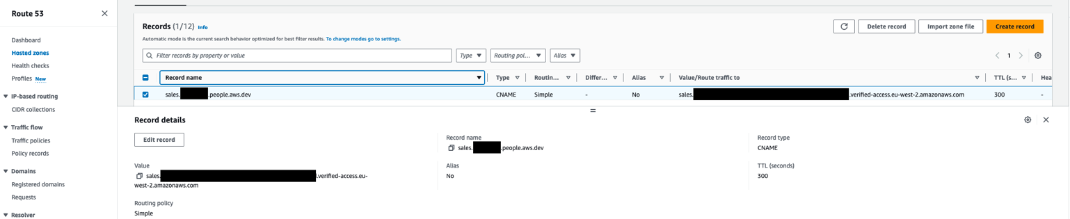
  7. In the Value section, provide the endpoint domain that you copied from Verified Access endpoints. Leave everything else as the default settings and choose Create records. Repeat these steps for the other endpoint and provide the relevant subdomain and value to the record.

Figure 11: The Route 53 record has been created

Figure 11: The Route 53 record has been created

And that’s it. You have finished integrating Jamf Trust and Jamf Pro with Verified Access, and your users can now access their applications using the above CNAMES from their managed computers.

Test the solution

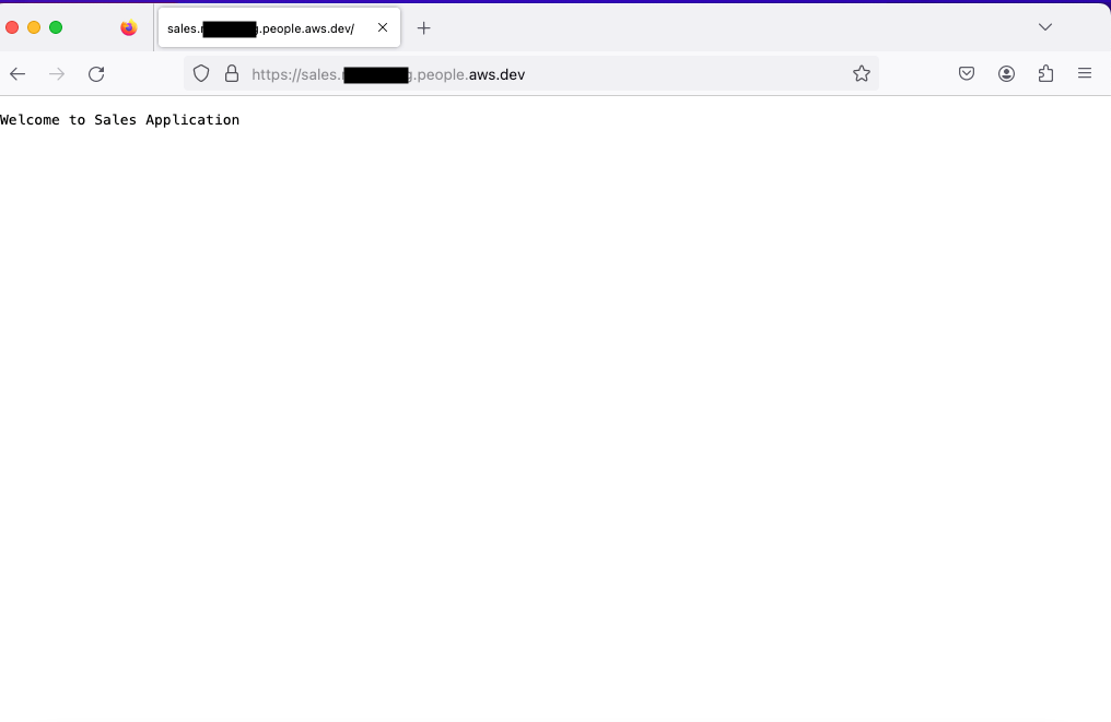
To test, use your browser (Firefox or Chrome) on one of your Jamf managed computers with the Verified Access extension installed to access one or both applications. The user will first be directed to the IAM Identity Center sign-in screen to sign in to the application. Then Verified Access will evaluate the user and the device posture before either granting or denying access to the user.

Figure 12: Access has been granted to the user based on identity and device posture

Figure 12: Access has been granted to the user based on identity and device posture

If the user meets the requirements, they will be presented with the application page. If the user doesn’t meet the requirements, they will receive a 403 Unauthorized error.

Figure 13: Access has been denied to the user based on identity and device posture

Figure 13: Access has been denied to the user based on identity and device posture

Troubleshooting on EC2 Mac

During testing or later, if your users receive a 403 Unauthorized error or the Verified Access extension isn’t forwarding the request, use the following steps to verify the browser extension being used and installed on the device is correct.

To verify the extension using Google Chrome:

  1. Verify that the browser extension is installed and is the latest version. If not, update the browser extension.
  2. Verify that Jamf Trust is installed and your device has the corresponding profiles for Jamf Trust. If not, install Jamf Trust and push the Jamf Trust profile to the device.
  3. If the problem persists, verify your local Jamf JSON configuration file and validate that the Chrome extension ID is correct. Follow these steps:
    1. Go to Chrome and select Manage Extensions.
    2. Enable Developer mode.
    3. Check the value of ID for your installed Verified Access browser extension.
    4. Open your terminal.
    5. Use the following command to change your directory to /Library/Google/Chrome/NativeMessagingHosts
      cd /Library/Google/Chrome/NativeMessagingHosts

    6. Verify that the value for chrome-extension matches the ID of the installed browser extension.

To verify the extension using Firefox:

  1. Verify that the browser extension is installed and is the latest version. If not, update the browser extension.
  2. Verify that Jamf Trust is installed and your device has the corresponding profiles for Jamf Trust. If not, install Jamf Trust and push the Jamf Trust profile to the device.
  3. If the problem persists, verify your local Jamf JSON configuration file and validate that it points to the correct Verified Access Firefox browser extension deployment.
    1. Open your terminal.
    2. Use the following command to change your directory to /Library/Application\ Support/Mozilla/NativeMessagingHosts:
      cd /Library/Application\ Support/Mozilla/NativeMessagingHosts

    3. Verify that the value for allowed_extensions is pointing to verified-access@amazonaws.

Conclusion

In this blog post, you learned how to use additional claims from a device trust provider such as Jamf in addition to user identity to provide access to corporate applications with AWS Verified Access. The access policies defined at Verified Access level consider the user identity and the device posture to determine and grant access to a user. Verified Access aligns with the principles of Zero Trust and evaluates each access request at scale in real time for user identity and device posture. Verified Access helps you keep your applications hosted in AWS securely without relying solely on a network perimeter for protection. To get started with Verified Access, visit the Amazon VPC console.

 
If you have feedback about this post, submit comments in the Comments section below. If you have questions about this post, contact AWS Support.
Want more AWS Security news? Follow us on Twitter.

Mayank Gupta

Mayank Gupta

Mayank is a senior technical account manager with AWS. With over 15 years of experience, Mayank’s expertise lies in cloud infrastructure, architecture, and security. He enjoys helping customers build scalable, resilient, highly available and secure applications. He is based in Glasgow, and his current interest lies in artificial intelligence and machine learning (AI/ML) technology.

Investigating lateral movements with Amazon Detective investigation and Security Lake integration

Post Syndicated from Yue Zhu original https://aws.amazon.com/blogs/security/investigating-lateral-movements-with-amazon-detective-investigation-and-security-lake-integration/

According to the MITRE ATT&CK framework, lateral movement consists of techniques that threat actors use to enter and control remote systems on a network. In Amazon Web Services (AWS) environments, threat actors equipped with illegitimately obtained credentials could potentially use APIs to interact with infrastructures and services directly, and they might even be able to use APIs to evade defenses and gain direct access to Amazon Elastic Compute Cloud (Amazon EC2) instances. To help customers secure their AWS environments, AWS offers several security services, such as Amazon GuardDuty, a threat detection service that monitors for malicious activity and anomalous behavior, and Amazon Detective, an investigation service that helps you investigate, and respond to, security events in your AWS environment.

After the service is turned on, Amazon Detective automatically collects logs from your AWS environment to help you analyze and investigate security events in-depth. At re:Invent 2023, Detective released Detective Investigations, a one-click investigation feature that automatically investigates AWS Identity and Access Management (IAM) users and roles for indicators of compromise (IoC), and Security Lake integration, which enables customers to retrieve log data from Amazon Security Lake to use as original evidence for deeper analysis with access to more detailed parameters.

In this post, you will learn about the use cases behind these features, how to run an investigation using the Detective Investigation feature, and how to interpret the contents of investigation reports. In addition, you will also learn how to use the Security Lake integration to retrieve raw logs to get more details of the impacted resources.

Triage a suspicious activity

As a security analyst, one of the common workflows in your daily job is to respond to suspicious activities raised by security event detection systems. The process might start when you get a ticket about a GuardDuty finding in your daily operations queue, alerting you that suspicious or malicious activity has been detected in your environment. To view more details of the finding, one of the options is to use the GuardDuty console.

In the GuardDuty console, you will find more details about the finding, such as the account and AWS resources that are in scope, the activity that caused the finding, the IP address that caused the finding and information about its possible geographic location, and times of the first and last occurrences of the event. To triage the finding, you might need more information to help you determine if it is a false positive.

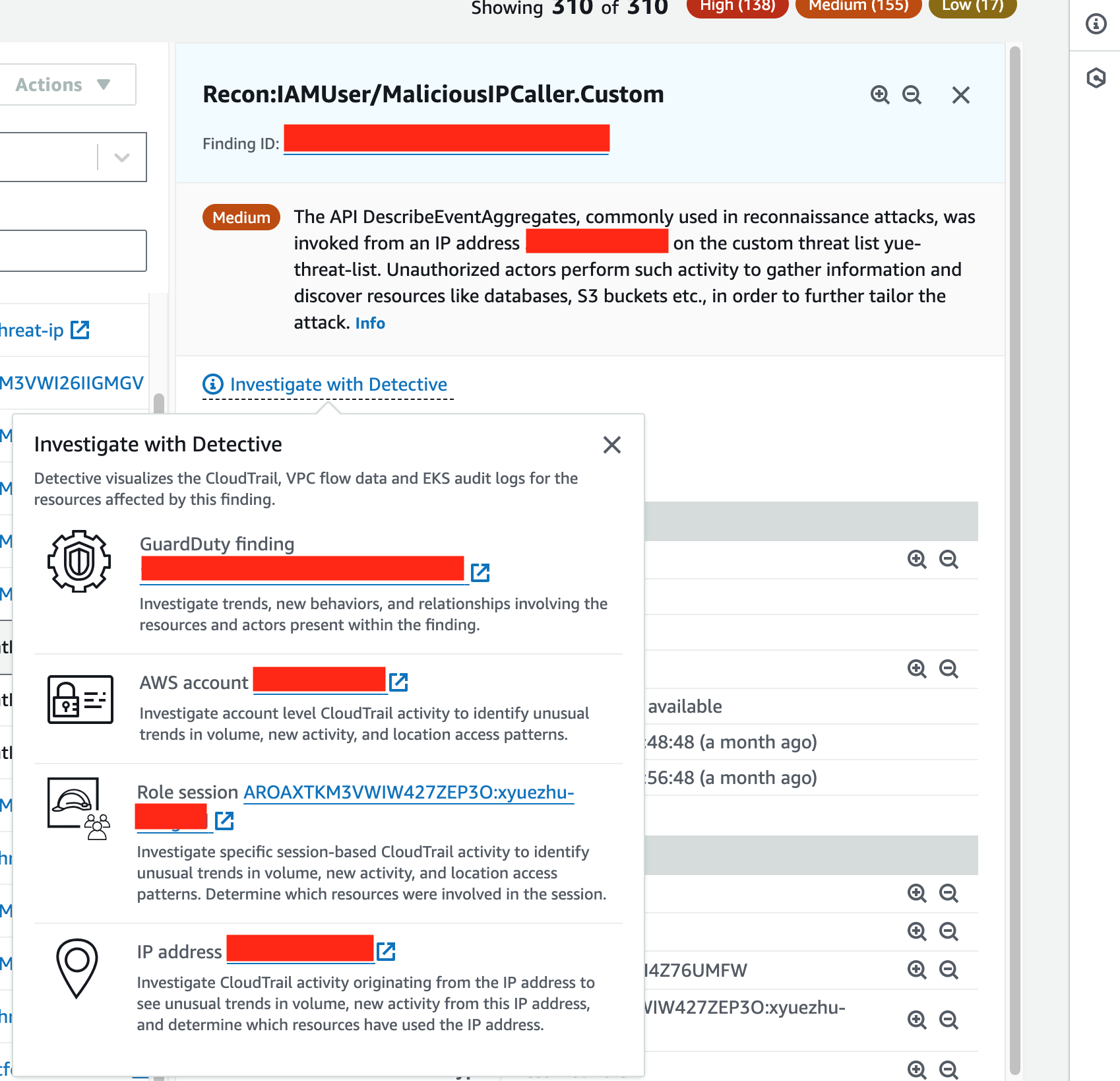
Every GuardDuty finding has a link labeled Investigate with Detective in the details pane. This link allows you to pivot to the Detective console based on aspects of the finding you are investigating to their respective entity profiles. The finding Recon:IAMUser/MaliciousIPCaller.Custom that’s shown in Figure 1 results from an API call made by an IP address that’s on the custom threat list, and GuardDuty observed it made API calls that were commonly used in reconnaissance activity, which commonly occurs prior to attempts at compromise. To investigate this finding, because it involves an IAM role, you can select the Role session link and it will take you to the role session’s profile in the Detective console.

Figure 1: Example finding in the GuardDuty console, with Investigate with Detective pop-up window

Figure 1: Example finding in the GuardDuty console, with Investigate with Detective pop-up window

Within the AWS Role session profile page, you will find security findings from GuardDuty and AWS Security Hub that are associated with the AWS role session, API calls the AWS role session made, and most importantly, new behaviors. Behaviors that deviate from expectations can be used as indicators of compromises to give you more information to determine if the AWS resource might be compromised. Detective highlights new behaviors first observed during the scope time of the events related to the finding that weren’t observed during the Detective baseline time window of 45 days.

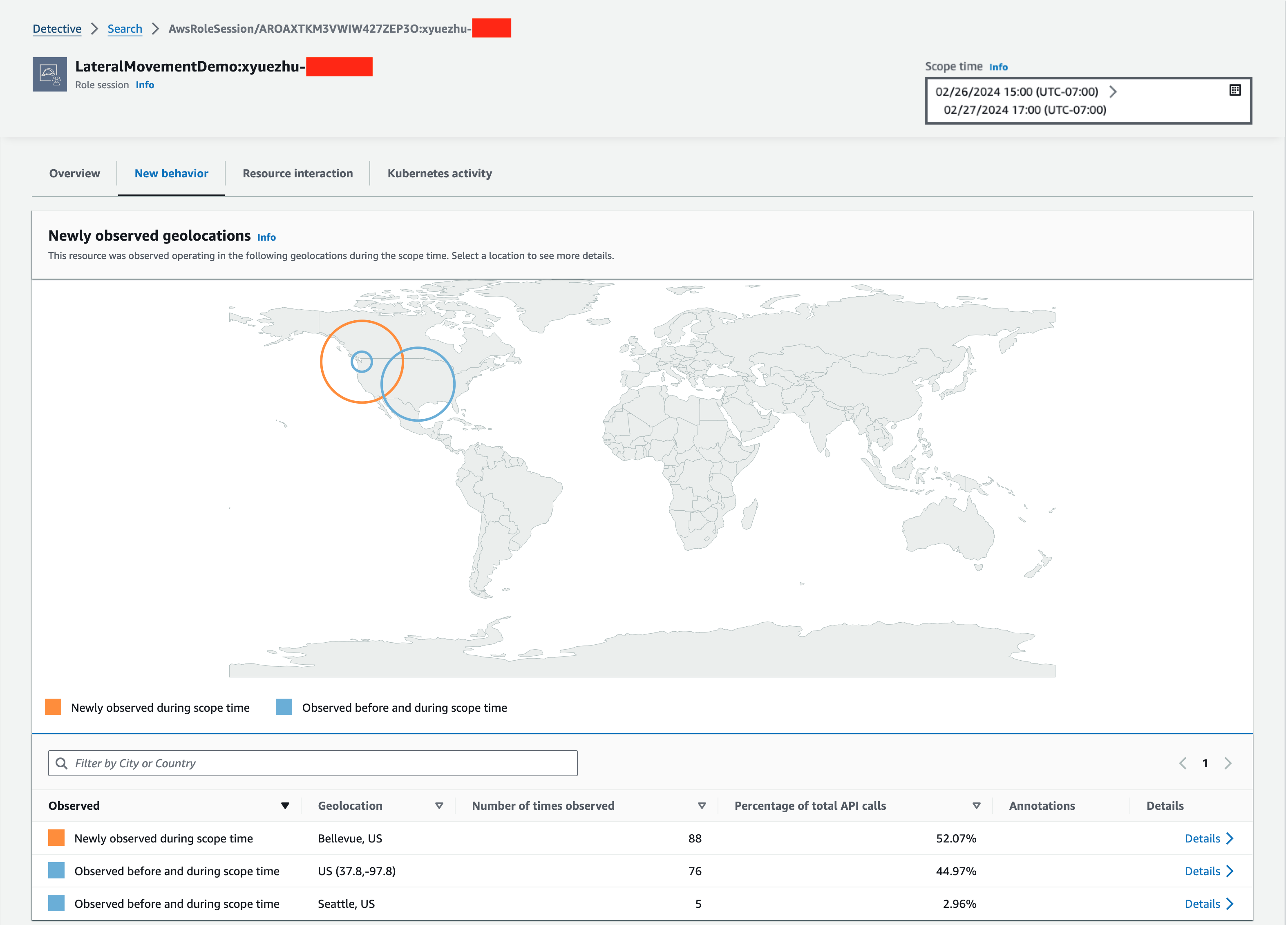
If you switch to the New behavior tab within the AWS role session profile, you will find the Newly observed geolocations panel (Figure 2). This panel highlights geolocations of IP addresses where API calls were made from that weren’t observed in the baseline profile. Detective determines the location of requests using MaxMind GeoIP databases based on the IP address that was used to issue requests.

Figure 2: Detective’s Newly observed geolocations panel

Figure 2: Detective’s Newly observed geolocations panel

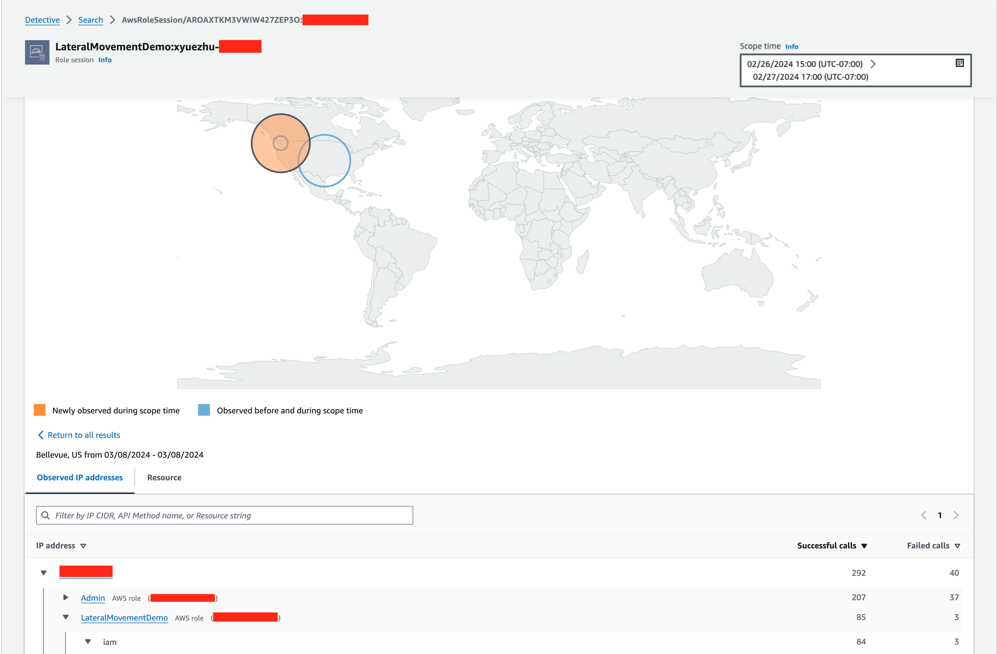
If you choose Details on the right side of each row, the row will expand and provide details of the API calls made from the same locations from different AWS resources, and you can drill down and get to the API calls made by the AWS resource from a specific geolocation (Figure 3). When analyzing these newly observed geolocations, a question you might consider is why this specific AWS role session made API calls from Bellevue, US. You’re pretty sure that your company doesn’t have a satellite office there, nor do your coworkers who have access to this role work from there. You also reviewed the AWS CloudTrail management events of this AWS role session, and you found some unusual API calls for services such as IAM.

Figure 3: Detective’s Newly observed geolocations panel expanded on details

Figure 3: Detective’s Newly observed geolocations panel expanded on details

You decide that you need to investigate further, because this role session’s anomalous behavior from a new geolocation is sufficiently unexpected, and it made unusual API calls that you would like to know the purpose of. You want to gather anomalous behaviors and high-risk API methods that can be used by threat actors to make impacts. Because you’re investigating an AWS role session rather than investigating a single role session, you decide you want to know what happened in other role sessions associated with the AWS role in case threat actors spread their activities across multiple sessions. To help you examine multiple role sessions automatically with additional analytics and threat intelligence, Detective introduced the Detective Investigation feature at re:Invent 2023.

Run an IAM investigation

Amazon Detective Investigation uses machine learning (ML) models and AWS threat intelligence to automatically analyze resources in your AWS environment to identify potential security events. It identifies tactics, techniques, and procedures (TTPs) used in a potential security event. The MITRE ATT&CK framework is used to classify the TTPs. You can use this feature to help you speed up the investigation and identify indicators of compromise and other TTPs quickly.

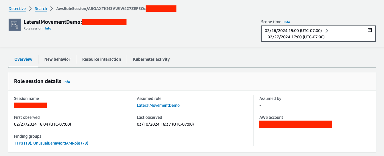
To continue with your investigation, you should investigate the role and its usage history as a whole to cover all involved role sessions at once. This addresses the potential case where threat actors assumed the same role under different session names. In the AWS role session profile page that’s shown in Figure 4, you can quickly identify and pivot to the corresponding AWS role profile page under the Assumed role field.

Figure 4: Detective’s AWS role session profile page

Figure 4: Detective’s AWS role session profile page

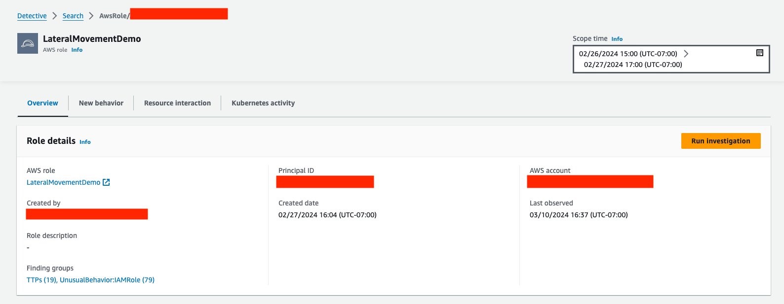
After you pivot to the AWS role profile page (Figure 5), you can run the automated investigations by choosing Run investigation.

Figure 5: Role profile page, from which an investigation can be run

Figure 5: Role profile page, from which an investigation can be run

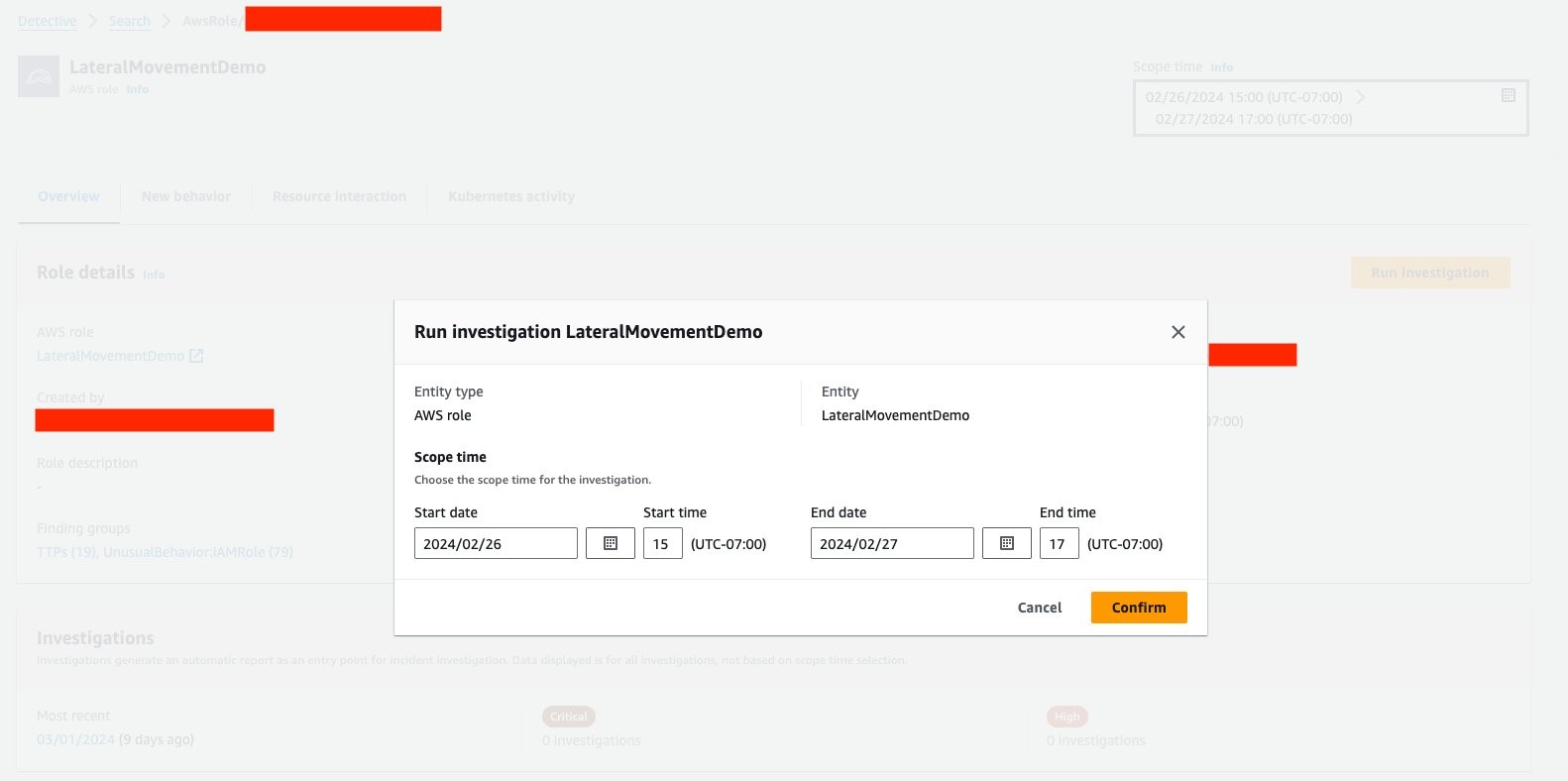
The first thing to do in a new investigation is to choose the time scope you want to run the investigation for. Then, choose Confirm (Figure 6).

Figure 6: Setting investigation scope time

Figure 6: Setting investigation scope time

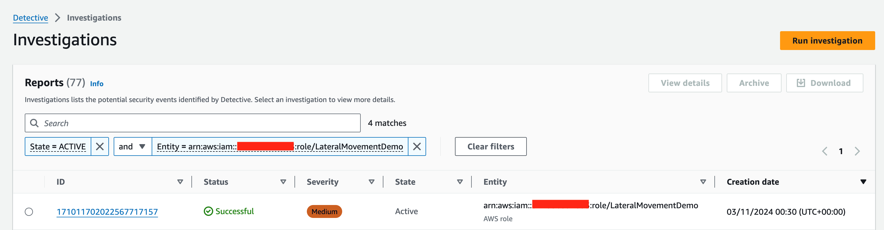
Next, you will be directed to the Investigations page (Figure 7), where you will be able to see the status of your investigation. Once the investigation is done, you can choose the hyperlinked investigation ID to access the investigation report.

Figure 7: Investigations page, with new report

Figure 7: Investigations page, with new report

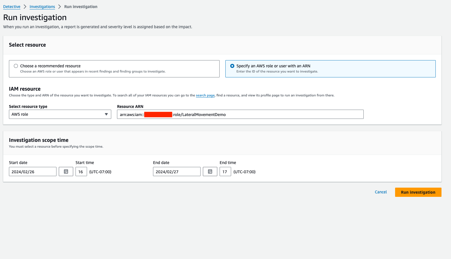
Another way to run an investigation is to choose Investigations on the left menu panel in the Detective console, and then choose Run investigation. You will then be taken to the page where you will specify the AWS role Amazon Resource Number (ARN) you’re investigating, and the scope time (Figure 8). Then you can choose Run investigation to commence an investigation.

Figure 8: Configuring a new investigation from scratch rather than from an existing finding

Figure 8: Configuring a new investigation from scratch rather than from an existing finding

Detective also offers StartInvestigation and GetInvestigation APIs for running Detective Investigations and retrieving investigation reports programmatically.

Interpret the investigation report

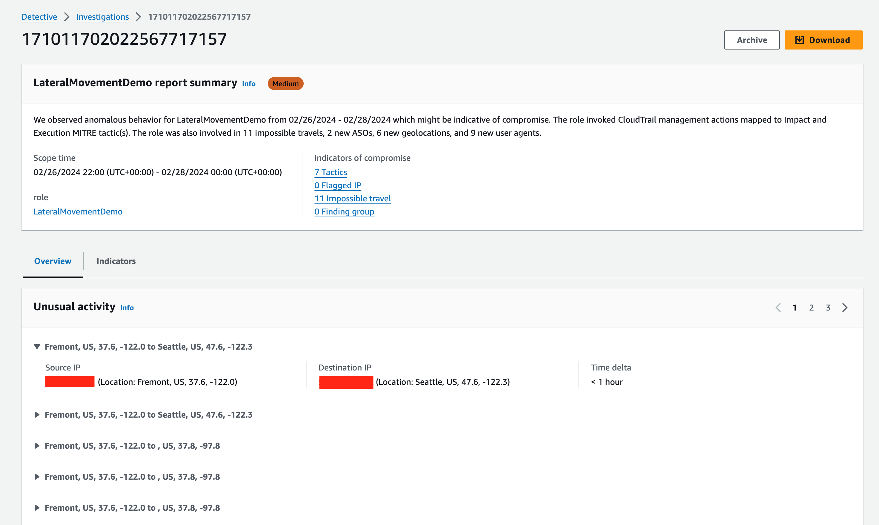
The investigation report (Figure 9) includes information on anomalous behaviors, potential TTP mappings of observed CloudTrail events, and indicators of compromises of the resource (in this example, an IAM principal) that was investigated.

At the top of the report, you will find a severity level computed based on the observed behaviors during the scope window, as well as a summary statement to give you a quick understanding of what was found. In Figure 9, the AWS role that was investigated engaged in the following unusual behaviors:

  • Seven tactics showing that the API calls made by this AWS role were mapped to seven tactics of the MITRE ATT&CK framework.
  • Eleven cases of impossible travel representing API calls made from two geolocations that are too far apart for the same user to have physically travelled between them to make the calls from both, within the time span involved.
  • Zero flagged IP addresses. Detective would flag IP addresses that are considered suspicious according to its threat intelligence sources.
  • Two new Autonomous System Organizations (ASOs) which are entities with assigned Autonomous System Numbers (ASNs) as used in Border Gateway Protocol (BGP) routing.
  • Nine new user agents were used to make API calls that weren’t observed in the 45 days prior to the events being investigated.

These indicators of compromise represent unusual behaviors that have either not been observed before in the AWS account involved or that are intrinsically considered high risk. The following summary panel includes the report that shows a detailed breakdown of the investigation results.

Unusual activities are important factors that you should look for during investigations, and sudden behavior change can be a sign of compromise. When you’re investigating an AWS role that can be assumed by different users from different AWS Regions, you are likely to need to examine activity at the granularity of the specific AWS role session that made the APIs calls. Within the report, you can do this by choosing the hyperlinked role name in the summary panel, and it will take you to the AWS role profile page.

Figure 9: Investigation report summary page

Figure 9: Investigation report summary page

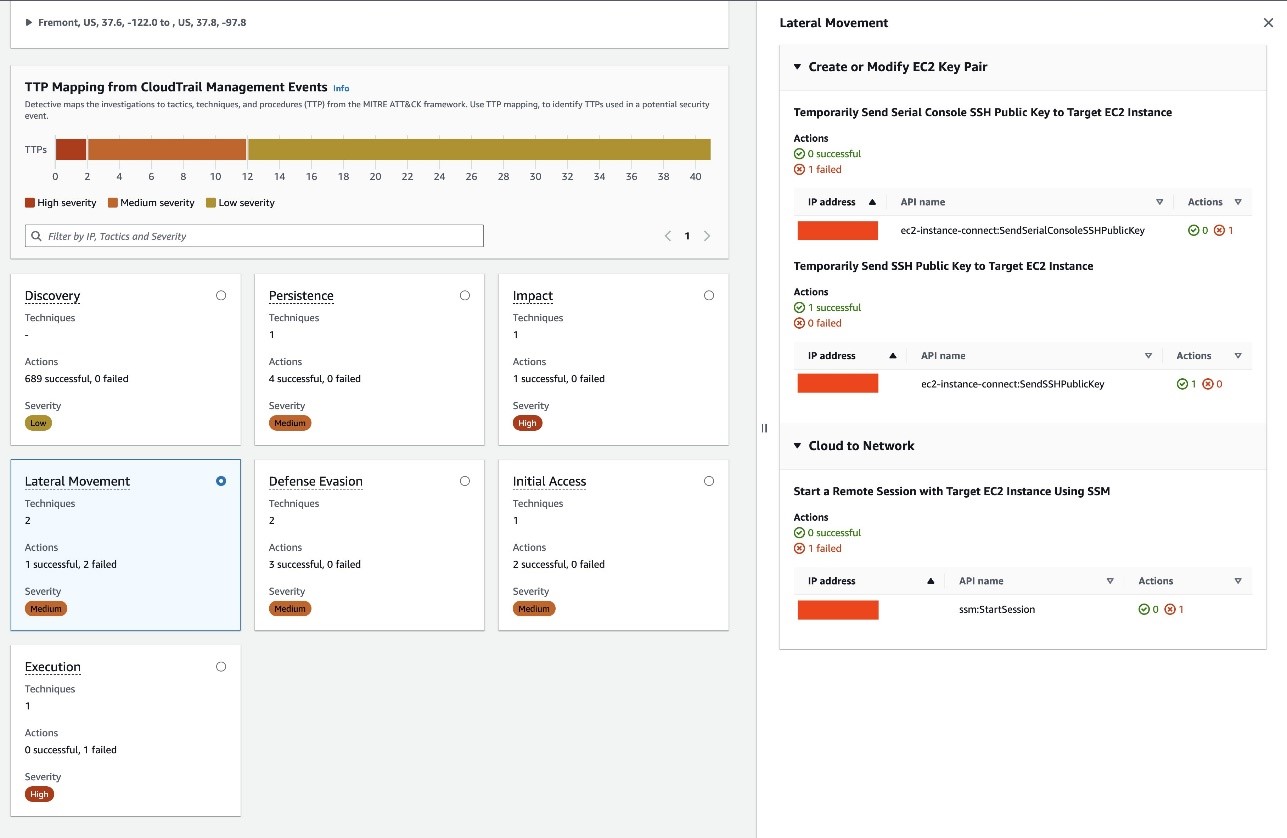
Further down on the investigation report is the TTP Mapping from CloudTrail Management Events panel. Detective Investigations maps CloudTrail events to the MITRE ATT&CK framework to help you understand how an API can be used by threat actors. For each mapped API, you can see the tactics, techniques, and procedures it can be used for. In Figure 10, at the top there is a summary of TTPs with different severity levels. At the bottom is a breakdown of potential TTP mappings of observed CloudTrail management events during the investigation scope time.

When you select one of the cards, a side panel appears on the right to give you more details about the APIs. It includes information such as the IP address that made the API call, the details of the TTP the API call was mapped to, and if the API call succeeded or failed. This information can help you understand how these APIs can potentially be used by threat actors to modify your environment, and whether or not the API call succeeded tells you if it might have affected the security of your AWS resources. In the example that’s shown in Figure 10, the IAM role successfully made API calls that are mapped to Lateral Movement in the ATT&CK framework.

Figure 10: Investigation report page with event ATT CK mapping

Figure 10: Investigation report page with event ATT CK mapping

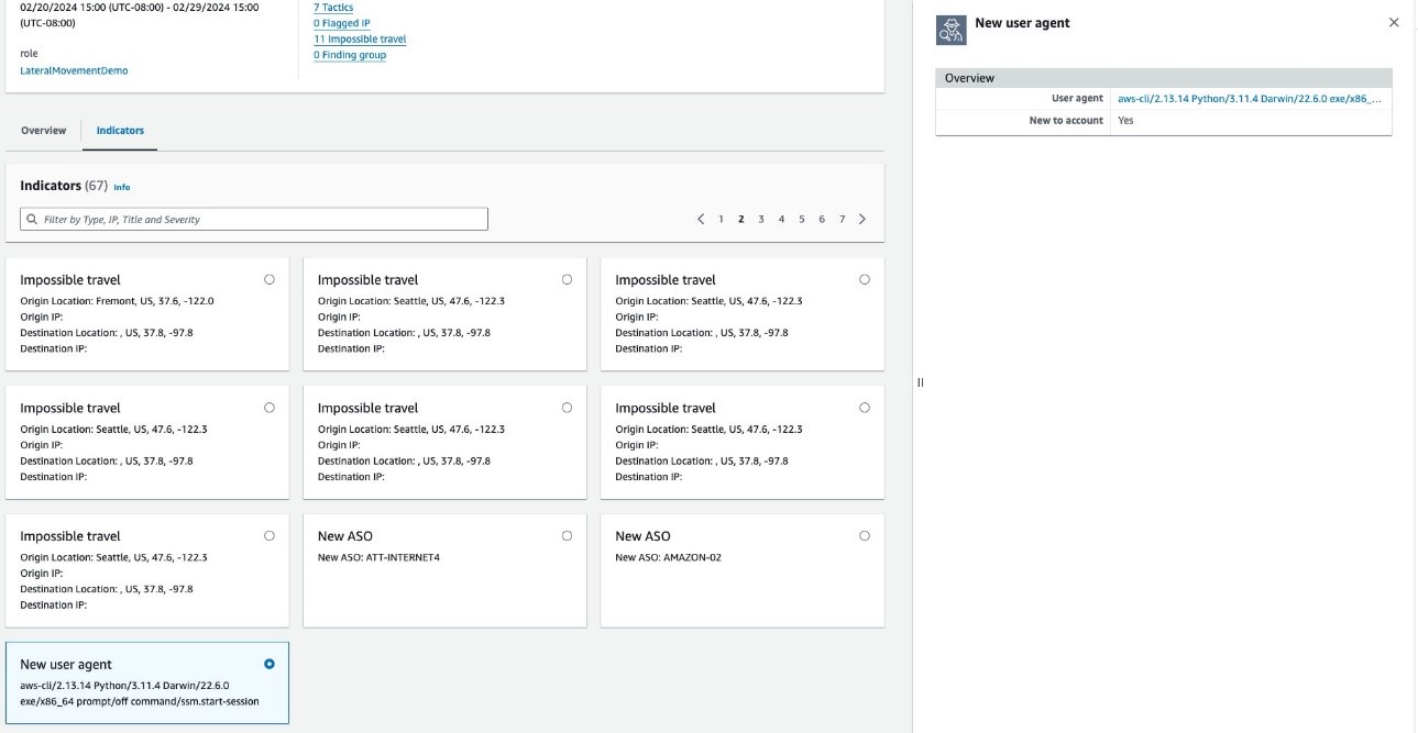
The report also includes additional indicators of compromise (Figure 11). You can find these if you select the Indicators tab next to Overview. Within this tab, you can find the indicators identified during the scope time, and if you select one indicator, details for that indicator will appear on the right. In the example in Figure 11, the IAM role made API calls with a user agent that wasn’t used by this IAM role or other IAM principals in this account, and indicators like this one show sudden behavior change of your IAM principal. You should review them and identify the ones that aren’t expected. To learn more about indicators of compromise in Detective Investigation, see the Amazon Detective User Guide.

Figure 11: Indicators of compromise identified during scope time

Figure 11: Indicators of compromise identified during scope time

At this point, you’ve analyzed the new and unusual behaviors the IAM role made and learned that the IAM role made API calls using new user agents and from new ASOs. In addition, you went through the API calls that were mapped to the MITRE ATT&CK framework. Among the TTPs, there were three API calls that are classified as lateral movements. These should attract attention for the following reasons: first, the purpose of these API calls is to gain access to the EC2 instance involved; and second, ec2-instance-connect:SendSSHPublicKey was run successfully.

Based on the procedure description in the report, this API would grant threat actors temporary SSH access to the target EC2 instance. To gather original evidence, examine the raw logs stored in Security Lake. Security Lake is a fully managed security data lake service that automatically centralizes security data from AWS environments, SaaS providers, on-premises sources, and other sources into a purpose-built data lake stored in your account.

Retrieve raw logs

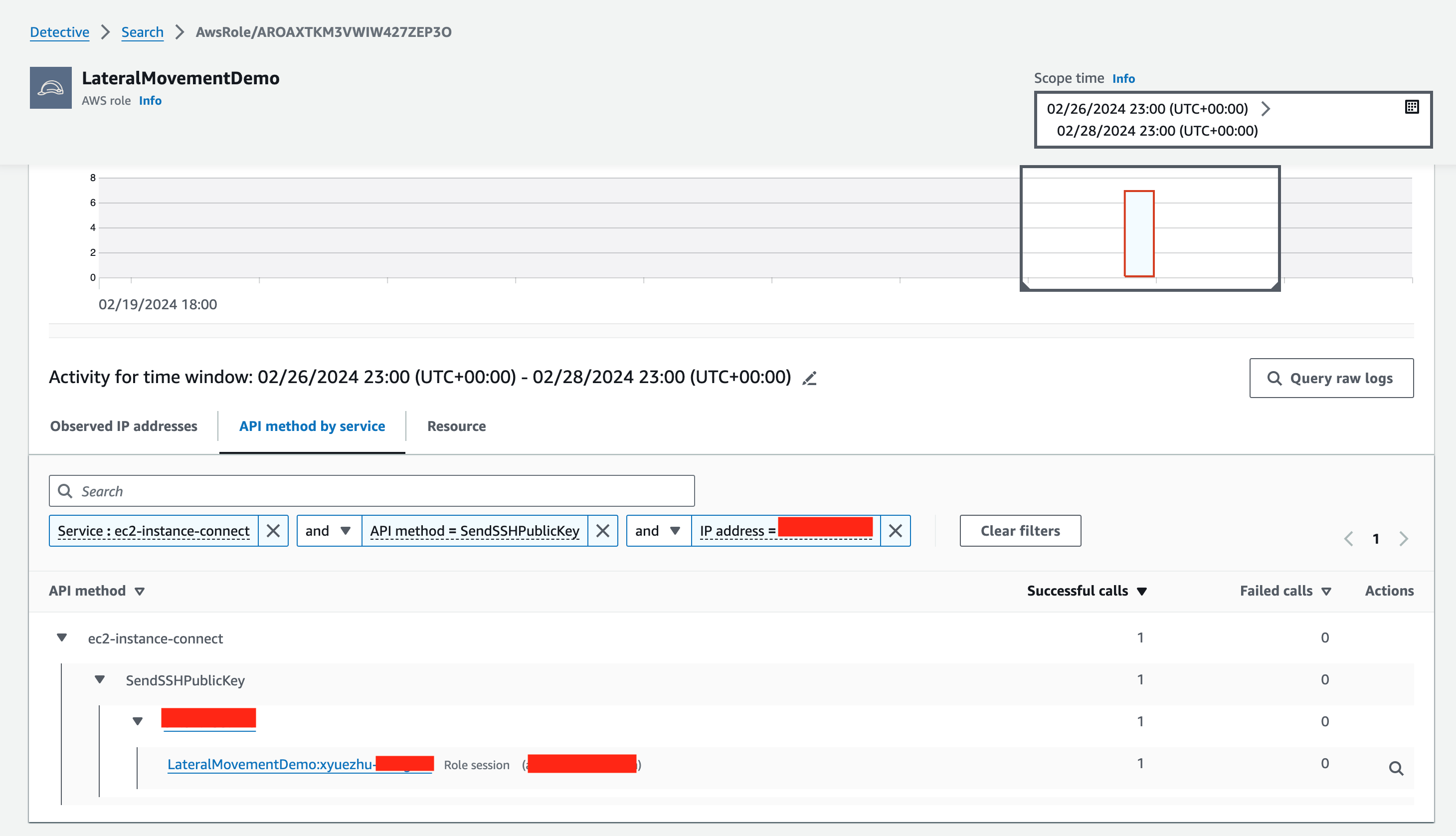
You can use Security Lake integration to retrieve raw logs from your Security Lake tables within the Detective console as original evidence. If you haven’t enabled the integration yet, you can follow the Integration with Amazon Security Lake guide to enable it. In the context of the example investigation earlier, these logs include details of which EC2 instance was associated with the ec2-instance-connect:SendSSHPublicKey API call. Within the AWS role profile page investigated earlier, if you scroll down to the bottom of the page, you will find the Overall API call volume panel (Figure 12). You can search for the specific API call using the Service and API method filters. Next, choose the magnifier icon, which will initiate a Security Lake query to retrieve the raw logs of the specific CloudTrail event.

Figure 12: Finding the CloudTrail record for a specific API call held in Security Lake

Figure 12: Finding the CloudTrail record for a specific API call held in Security Lake

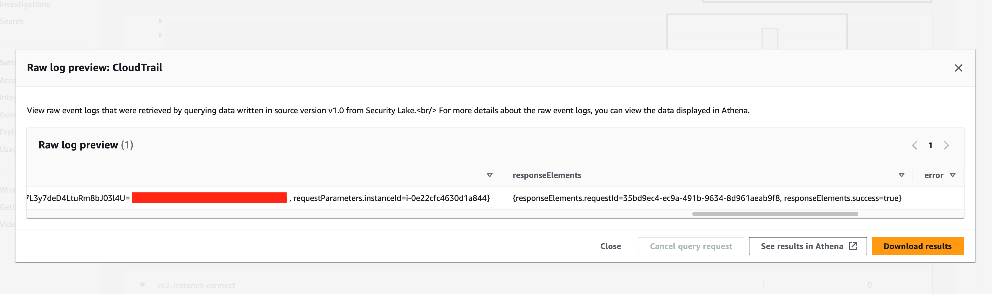
You can identify the target EC2 instance the API was issued against from the query results (Figure 13). To determine whether threat actors actually made an SSH connection to the target EC2 instance as a result of the API call, you should examine the EC2 instance’s profile page:

Figure 13: Reviewing a CloudTrail log record from Security Lake

Figure 13: Reviewing a CloudTrail log record from Security Lake

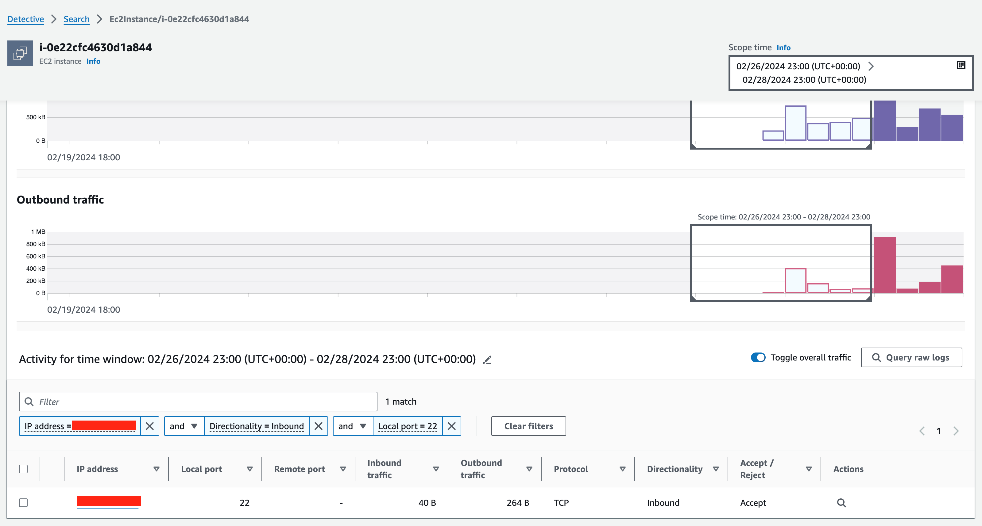
From the profile page of the EC2 instance in the Detective console, you can go to the Overall VPC flow volume panel and filter the Amazon Virtual Private Cloud (Amazon VPC) flow logs using the attributes related to the threat actor identified as having made the SSH API call. In Figure 14, you can see the IP address that tried to connect to 22/tcp, which is the SSH port of the target instance. It’s common for threat actors to change their IP address in an attempt to evade detection, and you can remove the IP address filter to see inbound connections to port 22/tcp of your EC2 instance.

Figure 14: Examining SSH connections to the target instance in the Detective profile page

Figure 14: Examining SSH connections to the target instance in the Detective profile page

Iterate the investigation

At this point, you’ve made progress with the help of Detective Investigations and Security Lake integration. You started with a GuardDuty finding, and you got to the point where you were able to identify some of the intent of the threat actors and uncover the specific EC2 instance they were targeting. Your investigation shouldn’t stop here because you’ve successfully identified the EC2 instance, which is the next target to investigate.

You can reuse this whole workflow by starting with the EC2 instance’s New behavior panel, run Detective Investigations on the IAM role attached to the EC2 instance and other IAM principals you think are worth taking a closer look at, then use the Security Lake integration to gather raw logs of the APIs made by the EC2 instance to identify the specific actions taken and their potential consequences.

Conclusion

In this post, you’ve seen how you can use the Amazon Detective Investigation feature to investigate IAM user and role activity and use the Security Lake integration to determine the specific EC2 instances a threat actor appeared to be targeting.

The Detective Investigation feature is automatically enabled for both existing and new customers in AWS Regions that support Detective where Detective has been activated. The Security Lake integration feature can be enabled in your Detective console. If you don’t currently use Detective, you can start a free 30-day trial. For more information on Detective Investigation and Security Lake integration, see Investigating IAM resources using Detective investigations and Security Lake integration.

 
If you have feedback about this post, submit comments in the Comments section below. If you have questions about this post, contact AWS Support.

Want more AWS Security news? Follow us on X.

Yue Zhu

Yue Zhu

Yue is a security engineer at AWS. Before AWS, he worked as a security engineer focused on threat detection, incident response, vulnerability management, and security tooling development. Outside of work, Yue enjoys reading, cooking, and cycling.

Revolutionizing data querying: Amazon Redshift and Visual Studio Code integration

Post Syndicated from Navnit Shukla original https://aws.amazon.com/blogs/big-data/revolutionizing-data-querying-amazon-redshift-and-visual-studio-code-integration/

In today’s data-driven landscape, the efficiency and accessibility of querying tools play a crucial role in driving businesses forward. Amazon Redshift recently announced integration with Visual Studio Code (), an action that transforms the way data practitioners engage with Amazon Redshift and reshapes your interactions and practices in data management. This innovation not only unlocks new possibilities, but also tackles long-standing challenges in data analytics and query handling.

While the Amazon Redshift query editor v2 (QE v2) offers a smooth experience for data analysts and business users, many organizations have data engineers and developers who rely on VS Code as their primary development tool. Traditionally, they had to use QE v2 for their development tasks, which wasn’t the most optimal solution. However, this new feature resolves that issue by enabling data engineers and developers to seamlessly integrate their development work within VS Code, enhancing their workflow efficiency.

Visual Studio Code’s integration simplifies access to database objects within Redshift data warehouses, offering an interface you’re already familiar with to run and troubleshoot your code.

By integrating Amazon Redshift Provisioned cluster, and Amazon Redshift Serverless with the popular and free VS Code, you can alleviate concerns about costs associated with third-party tools. This integration allows you to reduce or eliminate licensing expenses for query authoring and data visualization, because these functionalities are now available within the free VSCode editor.

The support for Amazon Redshift within VS Code marks a significant leap towards a more streamlined, cost-effective, and user-friendly data querying experience.

In this post, we explore how to kickstart your journey with Amazon Redshift using the AWS Toolkit for VS Code.

Solution overview

This post outlines the procedure for creating a secure and direct connection between your local VS Code environment and the Redshift cluster. Emphasizing both security and accessibility, this solution allows you to operate within the familiar VS Code interface while seamlessly engaging with your Redshift database.

The following diagram illustrates the VS Code connection to Amazon Redshift deployed in a private VPC.

To connect to a data warehouse using VS Code from the Toolkit, you can choose from the following methods:

  • Use a database user name and password
  • Use AWS Secrets Manager
  • Use temporary credentials (this option is only available with Amazon Redshift Provisioned cluster)

In the following sections, we show how to establish a connection with a database situated on an established provisioned cluster or a serverless data warehouse from the Toolkit.

Prerequisites

Before you begin using Amazon Redshift Provisioned Cluster  and Amazon Redshift Serverless with the AWS Toolkit for Visual Studio Code, make sure you’ve completed the following requirements:

  1. Connect to your AWS account using the Toolkit.
  2. Set up a Amazon Redshift or Amazon Redshift serverless data warehouse.

Establish a connection to your data warehouse using user credentials

To connect using the database user name and password, complete the following steps:

  1. Navigate through the Toolkit explorer, expanding the AWS Region housing your data warehouse (for example, US East (N. Virginia)).
  2. In the Toolkit, expand the Redshift section and choose your specific data warehouse.
  3. In the Select a Connection Type dialog, choose Database user name and password and provide the necessary information requested by the prompts.

After the Toolkit establishes the connection to your data warehouse, you will be able to view your available databases, tables, and schemas directly in the Toolkit explorer.

Establish a connection to your data warehouse using Secrets Manager

To connect using Secrets Manager, complete the following steps:

  1. Navigate through the Toolkit explorer, expanding the AWS Region housing your data warehouse.
  2. In the Toolkit, expand the Redshift section and choose your specific data warehouse.
  3. In the Select a Connection Type dialog, choose Secrets Manager and fill in the information requested at each prompt.

After the Toolkit establishes a successful connection to your data warehouse, you’ll gain visibility into your databases, tables, and schemas directly in the Toolkit explorer.

Establish a connection to your Amazon Redshift Provisioned cluster using Temporary credentials:

To connect using Temporary credentials complete the following steps:

  1. Navigate through the Toolkit explorer, expanding the AWS Region housing your data warehouse.
  2. In the Toolkit, expand the Redshift section and choose your specific data warehouse.
  3. In the Select a Connection Type dialog, choose Temporary Credentials and fill in the information requested at each prompt.

Run SQL statements

We have successfully established the connection. The next step involves running some SQL. The steps outlined in this section detail the process of generating and running SQL statements within your database using the Toolkit for Visual Studio Code.

  1. Navigate to the Toolkit explorer and expand Redshift, then choose the data warehouse that stores the desired database for querying.
  2. Choose Create Notebook and specify a file name and location for saving your notebook locally.
  3. Choose OK to open the notebook in your VS Code editor.
  4. Enter the following SQL statements into the VS Code editor, which will be stored in this notebook:
    create table promotion
    (
        p_promo_sk                integer               not null,
        p_promo_id                char(16)              not null,
        p_start_date_sk           integer                       ,
        p_end_date_sk             integer                       ,
        p_item_sk                 integer                       ,
        p_cost                    decimal(15,2)                 ,
        p_response_target         integer                       ,
        p_promo_name              char(50)                      ,
        p_channel_dmail           char(1)                       ,
        p_channel_email           char(1)                       ,
        p_channel_catalog         char(1)                       ,
        p_channel_tv              char(1)                       ,
        p_channel_radio           char(1)                       ,
        p_channel_press           char(1)                       ,
        p_channel_event           char(1)                       ,
        p_channel_demo            char(1)                       ,
        p_channel_details         varchar(100)                  ,
        p_purpose                 char(15)                      ,
        p_discount_active         char(1)                       ,
        primary key (p_promo_sk)
    ) diststyle all;
    
    create table reason
    (
        r_reason_sk               integer               not null,
        r_reason_id               char(16)              not null,
        r_reason_desc             char(100)                     ,
        primary key (r_reason_sk)
    ) diststyle all ;
    
    
    create table ship_mode
    (
        sm_ship_mode_sk           integer               not null,
        sm_ship_mode_id           char(16)              not null,
        sm_type                   char(30)                      ,
        sm_code                   char(10)                      ,
        sm_carrier                char(20)                      ,
        sm_contract               char(20)                      ,
        primary key (sm_ship_mode_sk)
    ) diststyle all;
    
    
    copy promotion from 's3://redshift-downloads/TPC-DS/2.13/1TB/promotion/' iam_role default gzip delimiter '|' EMPTYASNULL region 'us-east-1';
    copy reason from 's3://redshift-downloads/TPC-DS/2.13/1TB/reason/' iam_role default gzip delimiter '|' EMPTYASNULL region 'us-east-1';
    copy ship_mode from 's3://redshift-downloads/TPC-DS/2.13/1TB/ship_mode/' iam_role default gzip delimiter '|' EMPTYASNULL region 'us-east-1';
    
    
    select * from promotion limit 10;
    
    drop table promotion;
    drop table reason;
    drop table ship_mode;

  5. Choose Run All to run the SQL statements.

The output corresponding to your SQL statements will be visible below the entered statements within the editor.

Include markdown in a notebook

To include markdown in your notebook, complete the following steps:

  1. Access your notebook within the VS Code editor and choose Markdown to create a markdown cell.
  2. Enter your markdown content within the designated cell.
  3. Use the editing tools in the upper-right corner of the markdown cell to modify the markdown content as needed.

Congratulations, you have learned the art of using the VS Code editor to effectively interface with your Redshift environment.

Clean up

To remove the connection, complete the following steps:

  1. In the Toolkit explorer, expand Redshift, and choose the data warehouse containing your database.
  2. Choose the database (right-click) and choose Delete Connection.

Conclusion

In this post, we explored the process of using VS Code to establish a connection with Amazon Redshift, streamlining access to database objects within Redshift data warehouses.

You can learn about Amazon Redshift from Getting started with Amazon Redshift guide. Know more about write and run SQL queries directly in VS Code with the new AWS Toolkit for VS Code integration.


About the Author

Navnit Shukla, an AWS Specialist Solution Architect specializing in Analytics, is passionate about helping clients uncover valuable insights from their data. Leveraging his expertise, he develops inventive solutions that empower businesses to make informed, data-driven decisions. Notably, Navnit Shukla is the accomplished author of the book “Data Wrangling on AWS,” showcasing his expertise in the field.

Analyze more demanding as well as larger time series workloads with Amazon OpenSearch Serverless 

Post Syndicated from Satish Nandi original https://aws.amazon.com/blogs/big-data/analyze-more-demanding-as-well-as-larger-time-series-workloads-with-amazon-opensearch-serverless/

In today’s data-driven landscape, managing and analyzing vast amounts of data, especially logs, is crucial for organizations to derive insights and make informed decisions. However, handling this data efficiently presents a significant challenge, prompting organizations to seek scalable solutions without the complexity of infrastructure management.

Amazon OpenSearch Serverless lets you run OpenSearch in the AWS Cloud, without worrying about scaling infrastructure. With OpenSearch Serverless, you can ingest, analyze, and visualize your time-series data. Without the need for infrastructure provisioning, OpenSearch Serverless simplifies data management and enables you to derive actionable insights from extensive repositories.

We recently announced a new capacity level of 10TB for Time-series data per account per Region, which includes one or more indexes within a collection. With the support for larger datasets, you can unlock valuable operational insights and make data-driven decisions to troubleshoot application downtime, improve system performance, or identify fraudulent activities.

In this post, we discuss this new capability and how you can analyze larger time series datasets with OpenSearch Serverless.

10TB Time-series data size support in OpenSearch Serverless

The compute capacity for data ingestion and search or query in OpenSearch Serverless is measured in OpenSearch Compute Units (OCUs). These OCUs are shared among various collections, each containing one or more indexes within the account. To accommodate larger datasets, OpenSearch Serverless now supports up to 200 OCUs per account per AWS Region, each for indexing and search respectively, doubling from the previous limit of 100. You configure the maximum OCU limits on search and indexing independently to manage costs. You can also monitor real-time OCU usage with Amazon CloudWatch metrics to gain a better perspective on your workload’s resource consumption.

Dealing with larger data and analysis needs more memory and CPU. With 10TB data size support, OpenSearch Serverless is introducing vertical scaling up to eight times of 1-OCU systems. For example, the OpenSearch Serverless will deploy a larger system equivalent of eight 1-OCU systems. The system will use hybrid of horizontal and vertical scaling to address the needs of the workloads. There are improvements to shard reallocation algorithm to reduce the shard movement during heat remediation, vertical scaling, or routine deployment.

In our internal testing for 10TB Time-series data, we set the Max OCU to 48 for Search and 48 for Indexing. We set the data retention for 5 days using data lifecycle policies, and set the deployment type to “Enable redundancy” making sure the data is replicated across Availability Zones . This will lead to 12_24 hours of data in hot storage (OCU disk memory) and the rest in Amazon Simple Service (Amazon S3) storage. We observed the average ingestion achieved was 2.3 TiB per day with an average ingestion performance of 49.15 GiB per OCU per day, reaching a max of 52.47 GiB per OCU per day and a minimum of 32.69 Gib per OCU per day in our testing. The performance depends on several aspects, like document size, mapping, and other parameters, which may or may not have a variation for your workload.

Set max OCU to 200

You can start using our expanded capacity today by setting your OCU limits for indexing and search to 200. You can still set the limits to less than 200 to maintain a maximum cost during high traffic spikes. You only pay for the resources consumed, not for the max OCU configuration.

Ingest the data

You can use the load generation scripts shared in the following workshop, or you can use your own application or data generator to create a load. You can run multiple instances of these scripts to generate a burst in indexing requests. As shown in the following screenshot, we tested with an index, sending approximately 10 TB of data. We used our load generator script to send the traffic to a single index, retaining data for 5 days, and used a data life cycle policy to delete data older than 5 days.

Auto scaling in OpenSearch Serverless with new vertical scaling.

Before this release, OpenSearch Serverless auto-scaled by horizontally adding the same-size capacity to handle increases in traffic or load. With the new feature of vertical scaling to a larger size capacity, it can optimize the workload by providing a more powerful compute unit. The system will intelligently decide whether horizontal scaling or vertical scaling is more price-performance optimal. Vertical scaling also improves auto-scaling responsiveness, because vertical scaling helps to reach the optimal capacity faster compared to the incremental steps taken through horizontal scaling. Overall, vertical scaling has significantly improved the response time for auto_scaling.

Conclusion

We encourage you to take advantage of the 10TB index support and put it to the test! Migrate your data, explore the improved throughput, and take advantage of the enhanced scaling capabilities. Our goal is to deliver a seamless and efficient experience that aligns with your requirements.

To get started, refer to Log analytics the easy way with Amazon OpenSearch Serverless. To get hands-on experience with OpenSearch Serverless, follow the Getting started with Amazon OpenSearch Serverless workshop, which has a step-by-step guide for configuring and setting up an OpenSearch Serverless collection.

If you have feedback about this post, share it in the comments section. If you have questions about this post, start a new thread on the Amazon OpenSearch Service forum or contact AWS Support.


About the authors

Satish Nandi is a Senior Product Manager with Amazon OpenSearch Service. He is focused on OpenSearch Serverless and has years of experience in networking, security and ML/AI. He holds a Bachelor’s degree in Computer Science and an MBA in Entrepreneurship. In his free time, he likes to fly airplanes, hang gliders and ride his motorcycle.

Michelle Xue is Sr. Software Development Manager working on Amazon OpenSearch Serverless. She works closely with customers to help them onboard OpenSearch Serverless and incorporates customer’s feedback into their Serverless roadmap. Outside of work, she enjoys hiking and playing tennis.

Prashant Agrawal is a Sr. Search Specialist Solutions Architect with Amazon OpenSearch Service. He works closely with customers to help them migrate their workloads to the cloud and helps existing customers fine-tune their clusters to achieve better performance and save on cost. Before joining AWS, he helped various customers use OpenSearch and Elasticsearch for their search and log analytics use cases. When not working, you can find him traveling and exploring new places. In short, he likes doing Eat → Travel → Repeat.

Optimize data layout by bucketing with Amazon Athena and AWS Glue to accelerate downstream queries

Post Syndicated from Takeshi Nakatani original https://aws.amazon.com/blogs/big-data/optimize-data-layout-by-bucketing-with-amazon-athena-and-aws-glue-to-accelerate-downstream-queries/

In the era of data, organizations are increasingly using data lakes to store and analyze vast amounts of structured and unstructured data. Data lakes provide a centralized repository for data from various sources, enabling organizations to unlock valuable insights and drive data-driven decision-making. However, as data volumes continue to grow, optimizing data layout and organization becomes crucial for efficient querying and analysis.

One of the key challenges in data lakes is the potential for slow query performance, especially when dealing with large datasets. This can be attributed to factors such as inefficient data layout, resulting in excessive data scanning and inefficient use of compute resources. To address this challenge, common practices like partitioning and bucketing can significantly improve query performance and reduce computation costs.

Partitioning is a technique that divides a large dataset into smaller, more manageable parts based on specific criteria, such as date, region, or product category. By partitioning data, downstream analytical queries can skip irrelevant partitions, reducing the amount of data that needs to be scanned and processed. You can use partition columns in the WHERE clause in queries to scan only the specific partitions that your query needs. This can lead to faster query runtimes and more efficient resource utilization. It especially works well when columns with low cardinality are chosen as the key.

What if you have a high cardinality column that you sometimes need to filter by VIP customers? Each customer is usually identified with an ID, which can be millions. Partitioning isn’t suitable for such high cardinality columns because you end up with small files, slow partition filtering, and high Amazon Simple Storage Service (Amazon S3) API cost (one S3 prefix is created per value of partition column). Although you can use partitioning with a natural key such as city or state to narrow down your dataset to some degree, it is still necessary to query across date-based partitions if your data is time series.

This is where bucketing comes into play. Bucketing makes sure that all rows with the same values of one or more columns end up in the same file. Instead of one file per value, like partitioning, a hash function is used to distribute values evenly across a fixed number of files. By organizing data this way, you can perform efficient filtering, because only the relevant buckets need to be processed, further reducing computational overhead.

There are multiple options for implementing bucketing on AWS. One approach is to use the Amazon Athena CREATE TABLE AS SELECT (CTAS) statement, which allows you to create a bucketed table directly from a query. Alternatively, you can use AWS Glue for Apache Spark, which provides built-in support for bucketing configurations during the data transformation process. AWS Glue allows you to define bucketing parameters, such as the number of buckets and the columns to bucket on, providing an optimized data layout for efficient querying with Athena.

In this post, we discuss how to implement bucketing on AWS data lakes, including using Athena CTAS statement and AWS Glue for Apache Spark. We also cover bucketing for Apache Iceberg tables.

Example use case

In this post, you use a public dataset, the NOAA Integrated Surface Database. Data analysts run one-time queries for data during the past 5 years through Athena. Most of the queries are for specific stations with specific report types. The queries need to complete in 10 seconds, and the cost needs to be optimized carefully. In this scenario, you’re a data engineer responsible for optimizing query performance and cost.

For example, if an analyst wants to retrieve data for a specific station (for example, station ID 123456) with a particular report type (for example, CRN01), the query might look like the following query:

SELECT station, report_type, columnA, columnB, ...
FROM table_name
WHERE
report_type = 'CRN01'
AND station = '123456'

In the case of the NOAA Integrated Surface Database, the station_id column is likely to have a high cardinality, with numerous unique station identifiers. On the other hand, the report_type column may have a relatively low cardinality, with a limited set of report types. Given this scenario, it would be a good idea to partition the data by report_type and bucket it by station_id.

With this partitioning and bucketing strategy, Athena can first eliminate partitions for irrelevant report types, and then scan only the buckets within the relevant partition that match the specified station ID, significantly reducing the amount of data processed and accelerating query runtimes. This approach not only meets the query performance requirement, but also helps optimize costs by minimizing the amount of data scanned and billed for each query.

In this post, we examine how query performance is affected by data layout, in particular, bucketing. We also compare three different ways to achieve bucketing. The following table represents conditions for the tables to be created.

. noaa_remote_original athena_non_bucketed athena_bucketed glue_bucketed athena_bucketed_iceberg
Format CSV Parquet Parquet Parquet Parquet
Compression n/a Snappy Snappy Snappy Snappy
Created via n/a Athena CTAS Athena CTAS Glue ETL Athena CTAS with Iceberg
Engine n/a Trino Trino Apache Spark Apache Iceberg
Is partitioned? Yes but with different way Yes Yes Yes Yes
Is bucketed? No No Yes Yes Yes

noaa_remote_original is partitioned by the year column, but not by the report_type column. This row represents if the table is partitioned by the actual columns that are used in the queries.

Baseline table

For this post, you create several tables with different conditions: some without bucketing and some with bucketing, to showcase the performance characteristics of bucketing. First, let’s create an original table using the NOAA data. In subsequent steps, you ingest data from this table to create test tables.

There are multiple ways to define a table definition: running DDL, an AWS Glue crawler, the AWS Glue Data Catalog API, and so on. In this step, you run DDL via the Athena console.

Complete the following steps to create the "bucketing_blog"."noaa_remote_original" table in the Data Catalog:

  1. Open the Athena console.
  2. In the query editor, run the following DDL to create a new AWS Glue database:
    -- Create Glue database
    CREATE DATABASE bucketing_blog;

  3. For Database under Data, choose bucketing_blog to set the current database.
  4. Run the following DDL to create the original table:
    -- Create original table
    CREATE EXTERNAL TABLE `bucketing_blog`.`noaa_remote_original`(
      `station` STRING, 
      `date` STRING, 
      `source` STRING, 
      `latitude` STRING, 
      `longitude` STRING, 
      `elevation` STRING, 
      `name` STRING, 
      `report_type` STRING, 
      `call_sign` STRING, 
      `quality_control` STRING, 
      `wnd` STRING, 
      `cig` STRING, 
      `vis` STRING, 
      `tmp` STRING, 
      `dew` STRING, 
      `slp` STRING, 
      `aj1` STRING, 
      `gf1` STRING, 
      `mw1` STRING)
    PARTITIONED BY (
        year STRING)
    ROW FORMAT SERDE 
      'org.apache.hadoop.hive.serde2.OpenCSVSerde' 
    WITH SERDEPROPERTIES ( 
      'escapeChar'='\\',
      'quoteChar'='\"',
      'separatorChar'=',') 
    STORED AS INPUTFORMAT 
      'org.apache.hadoop.mapred.TextInputFormat' 
    OUTPUTFORMAT 
      'org.apache.hadoop.hive.ql.io.HiveIgnoreKeyTextOutputFormat'
    LOCATION
      's3://noaa-global-hourly-pds/'
    TBLPROPERTIES (
      'skip.header.line.count'='1'
    )

Because the source data has quoted fields, we use OpenCSVSerde instead of the default LazySimpleSerde.

These CSV files have a header row, which we tell Athena to skip by adding skip.header.line.count and setting the value to 1.

For more details, refer to OpenCSVSerDe for processing CSV.

  1. Run the following DDL to add partitions. We add partitions only for 5 years out of 124 years based on the use case requirement:
    -- Load partitions
    ALTER TABLE `bucketing_blog`.`noaa_remote_original` ADD
      PARTITION (year = '2024') LOCATION 's3://noaa-global-hourly-pds/2024/'
      PARTITION (year = '2023') LOCATION 's3://noaa-global-hourly-pds/2023/'
      PARTITION (year = '2022') LOCATION 's3://noaa-global-hourly-pds/2022/'
      PARTITION (year = '2021') LOCATION 's3://noaa-global-hourly-pds/2021/'
      PARTITION (year = '2020') LOCATION 's3://noaa-global-hourly-pds/2020/';

  2. Run the following DML to verify if you can successfully query the data:
    -- Check data 
    SELECT * FROM "bucketing_blog"."noaa_remote_original" LIMIT 10;

Now you’re ready to start querying the original table to examine the baseline performance.

  1. Run a query against the original table to evaluate the query performance as a baseline. The following query selects records for five specific stations with report type CRN05:
    -- Baseline
    SELECT station, report_type, date, source, latitude, longitude, elevation, name, call_sign, quality_control, wnd, cig, tmp
    FROM "bucketing_blog"."noaa_remote_original"
    WHERE
        report_type = 'CRN05'
        AND ( station = '99999904237'
            OR station = '99999953132'
            OR station = '99999903061'
            OR station = '99999963856'
            OR station = '99999994644'
        );

We ran this query 10 times. The average query runtime for 10 queries is 27.6 seconds, which is far longer than our target of 10 seconds, and 155.75 GB data is scanned to return 1.65 million records. This is the baseline performance of the original raw table. It’s time to start optimizing data layout from this baseline.

Next, you create tables with different conditions from the original: one without bucketing and one with bucketing, and compare them.

Optimize data layout using Athena CTAS

In this section, we use an Athena CTAS query to optimize data layout and its format.

First, let’s create a table with partitioning but without bucketing. The new table is partitioned by the column report_type because most of expected queries use this column in the WHERE clause, and objects are stored as Parquet with Snappy compression.

  1. Open the Athena query editor.
  2. Run the following query, providing your own S3 bucket and prefix:
    --CTAS, non-bucketed
    CREATE TABLE "bucketing_blog"."athena_non_bucketed"
    WITH (
        external_location = 's3://<your-s3-location>/athena-non-bucketed/',
        partitioned_by = ARRAY['report_type'],
        format = 'PARQUET',
        write_compression = 'SNAPPY'
    )
    AS
    SELECT
        station, date, source, latitude, longitude, elevation, name, call_sign, quality_control, wnd, cig, vis, tmp, dew, slp, aj1, gf1, mw1, report_type
    FROM "bucketing_blog"."noaa_remote_original"
    ;

Your data should look like the following screenshots.


There are 30 files under the partition.

Next, you create a table with Hive style bucketing. The number of buckets needs to be carefully tuned through experiments for your own use case. Generally speaking, the more buckets you have, the smaller the granularity, which might result in better performance. On the other hand, too many small files may introduce inefficiency in query planning and processing. Also, bucketing only works if you are querying a few values of the bucketing key. The more values you add to your query, the more likely that you will end up reading all buckets.

The following is the baseline query to optimize:

-- Baseline
SELECT station, report_type, date, source, latitude, longitude, elevation, name, call_sign, quality_control, wnd, cig, tmp
FROM "bucketing_blog"."noaa_remote_original"
WHERE
    report_type = 'CRN05'
    AND ( station = '99999904237'
        OR station = '99999953132'
        OR station = '99999903061'
        OR station = '99999963856'
        OR station = '99999994644'
    );

In this example, the table is going to be bucketed into 16 buckets by a high-cardinality column (station), which is supposed to be used for the WHERE clause in the query. All other conditions remain the same. The baseline query has five values in the station ID, and you expect queries to have around that number at most, which is less enough than the number of buckets, so 16 should work well. It is possible to specify a larger number of buckets, but CTAS can’t be used if the total number of partitions exceeds 100.

  1. Run the following query:
    -- CTAS, Hive-bucketed
    CREATE TABLE "bucketing_blog"."athena_bucketed"
    WITH (
        external_location = 's3://<your-s3-location>/athena-bucketed/',
        partitioned_by = ARRAY['report_type'],
        bucketed_by = ARRAY['station'],
        bucket_count = 16,
        format = 'PARQUET',
        write_compression = 'SNAPPY'
    )
    AS
    SELECT
        station, date, source, latitude, longitude, elevation, name, call_sign, quality_control, wnd, cig, vis, tmp, dew, slp, aj1, gf1, mw1, report_type
    FROM "bucketing_blog"."noaa_remote_original"
    ;

The query creates S3 objects organized as shown in the following screenshots.


The table-level layout looks exactly the same between athena_non_bucketed and athena_bucketed: there are 13 partitions in each table. The difference is the number of objects under the partitions. There are 16 objects (buckets) per partition, of roughly 10–25 MB each in this case. The number of buckets is constant at the specified value regardless of the amount of data, but the bucket size depends on the amount of data.

Now you’re ready to query against each table to evaluate query performance. The query will select records with five specific stations and report type CRN05 for the past 5 years. Although you can’t see which data of a specific station is located in which bucket, it has been calculated and located correctly by Athena.

  1. Query the non-bucketed table with the following statement:
    -- No bucketing 
    SELECT station, report_type, date, source, latitude, longitude, elevation, name, call_sign, quality_control, wnd, cig, tmp
    FROM "bucketing_blog"."athena_non_bucketed"
    WHERE
        report_type = 'CRN05'
        AND ( station = '99999904237'
            OR station = '99999953132'
            OR station = '99999903061'
            OR station = '99999963856'
            OR station = '99999994644'
        );


We ran this query 10 times. The average runtime of the 10 queries is 10.95 seconds, and 358 MB of data is scanned to return 2.21 million records. Both the runtime and scan size have been significantly decreased because you’ve partitioned the data, and can now read only one partition where 12 partitions of 13 are skipped. In addition, the amount of data scanned has gone down from 206 GB to 360 MB, which is a reduction of 99.8%. This is not just due to the partitioning, but also due to the change of its format to Parquet and compression with Snappy.

  1. Query the bucketed table with the following statement:
    -- Hive bucketing
    SELECT station, report_type, date, source, latitude, longitude, elevation, name, call_sign, quality_control, wnd, cig, tmp
    FROM "bucketing_blog"."athena_bucketed"
    WHERE
        report_type = 'CRN05'
        AND ( station = '99999904237'
            OR station = '99999953132'
            OR station = '99999903061'
            OR station = '99999963856'
            OR station = '99999994644'
        );


We ran this query 10 times. The average runtime of the 10 queries is 7.82 seconds, and 69 MB of data is scanned to return 2.21 million records. This means a reduction of average runtime from 10.95 to 7.82 seconds (-29%), and a dramatic reduction of data scanned from 358 MB to 69 MB (-81%) to return the same number of records compared with the non-bucketed table. In this case, both runtime and data scanned were improved by bucketing. This means bucketing contributed not only to performance but also to cost reduction.

Considerations

As stated earlier, size your bucket carefully to maximize performance of your query. Bucketing only works if you are querying a few values of the bucketing key. Consider creating more buckets than the number of values expected in the actual query.

Additionally, an Athena CTAS query is limited to create up to 100 partitions at one time. If you need a large number of partitions, you may want to use AWS Glue extract, transform, and load (ETL), although there is a workaround to split into multiple SQL statements.

Optimize data layout using AWS Glue ETL

Apache Spark is an open source distributed processing framework that enables flexible ETL with PySpark, Scala, and Spark SQL. It allows you to partition and bucket your data based on your requirements. Spark has several tuning options to accelerate jobs. You can effortlessly automate and monitor Spark jobs. In this section, we use AWS Glue ETL jobs to run Spark code to optimize data layout.

Unlike Athena bucketing, AWS Glue ETL uses Spark-based bucketing as a bucketing algorithm. All you need to do is add the following table property onto the table: bucketing_format = 'spark'. For details about this table property, see Partitioning and bucketing in Athena.

Complete the following steps to create a table with bucketing through AWS Glue ETL:

  1. On the AWS Glue console, choose ETL jobs in the navigation pane.
  2. Choose Create job and choose Visual ETL.
  3. Under Add nodes, choose AWS Glue Data Catalog for Sources.
  4. For Database, choose bucketing_blog.
  5. For Table, choose noaa_remote_original.
  6. Under Add nodes, choose Change Schema for Transforms.
  7. Under Add nodes, choose Custom Transform for Transforms.
  8. For Name, enter ToS3WithBucketing.
  9. For Node parents, choose Change Schema.
  10. For Code block, enter the following code snippet:
    def ToS3WithBucketing (glueContext, dfc) -> DynamicFrameCollection:
        # Convert DynamicFrame to DataFrame
        df = dfc.select(list(dfc.keys())[0]).toDF()
        
        # Write to S3 with bucketing and partitioning
        df.repartition(1, "report_type") \
            .write.option("path", "s3://<your-s3-location>/glue-bucketed/") \
            .mode("overwrite") \
            .partitionBy("report_type") \
            .bucketBy(16, "station") \
            .format("parquet") \
            .option("compression", "snappy") \
            .saveAsTable("bucketing_blog.glue_bucketed")

The following screenshot shows the job created using AWS Glue Studio to generate a table and data.

Each node represents the following:

  • The AWS Glue Data Catalog node loads the noaa_remote_original table from the Data Catalog
  • The Change Schema node makes sure that it loads columns registered in the Data Catalog
  • The ToS3WithBucketing node writes data to Amazon S3 with both partitioning and Spark-based bucketing

The job has been successfully authored in the visual editor.

  1. Under Job details, for IAM Role, choose your AWS Identity and Access Management (IAM) role for this job.
  2. For Worker type, choose G.8X.
  3. For Requested number of workers, enter 5.
  4. Choose Save, then choose Run.

After these steps, the table glue_bucketed. has been created.

  1. Choose Tables in the navigation pane, and choose the table glue_bucketed.
  2. On the Actions menu, choose Edit table under Manage.
  3. In the Table properties section, choose Add.
  4. Add a key pair with key bucketing_format and value spark.
  5. Choose Save.

Now it’s time to query the tables.

  1. Query the bucketed table with the following statement:
    -- Spark bucketing
    SELECT station, report_type, date, source, latitude, longitude, elevation, name, call_sign, quality_control, wnd, cig, tmp
    FROM "bucketing_blog"."glue_bucketed"
    WHERE
        report_type = 'CRN05'
        AND ( station = '99999904237'
            OR station = '99999953132'
            OR station = '99999903061'
            OR station = '99999963856'
            OR station = '99999994644'
        );


We ran the query 10 times. The average runtime of the 10 queries is 7.09 seconds, and 88 MB of data is scanned to return 2.21 million records. In this case, both the runtime and data scanned were improved by bucketing. This means bucketing contributed not only to performance but also to cost reduction.

The reason for the larger bytes scanned compared to the Athena CTAS example is that the values were distributed differently in this table. In the AWS Glue bucketed table, the values were distributed over five files. In the Athena CTAS bucketed table, the values were distributed over four files. Remember that rows are distributed into buckets using a hash function. The Spark bucketing algorithm uses a different hash function than Hive, and in this case, it resulted in a different distribution across the files.

Considerations

Glue DynamicFrame does not support bucketing natively. You need to use Spark DataFrame instead of DynamicFrame to bucket tables.

For information about fine-tuning AWS Glue ETL performance, refer to Best practices for performance tuning AWS Glue for Apache Spark jobs.

Optimize Iceberg data layout with hidden partitioning

Apache Iceberg is a high-performance open table format for huge analytic tables, bringing the reliability and simplicity of SQL tables to big data. Recently, there has been a huge demand to use Apache Iceberg tables to achieve advanced capabilities like ACID transaction, time travel query, and more.

In Iceberg, bucketing works differently than the Hive table method we’ve seen so far. In Iceberg, bucketing is a subset of partitioning, and can be applied using the bucket partition transform. The way you use it and the end result is similar to bucketing in Hive tables. For more details about Iceberg bucket transforms, refer to Bucket Transform Details.

Complete the following steps:

  1. Open the Athena query editor.
  2. Run the following query to create an Iceberg table with hidden partitioning along with bucketing:
    -- CTAS, Iceberg-bucketed
    CREATE TABLE "bucketing_blog"."athena_bucketed_iceberg"
    WITH (table_type = 'ICEBERG',
          location = 's3://<your-s3-location>/athena-bucketed-iceberg/', 
          is_external = false,
          partitioning = ARRAY['report_type', 'bucket(station, 16)'],
          format = 'PARQUET',
          write_compression = 'SNAPPY'
    ) 
    AS
    SELECT
        station, date, source, latitude, longitude, elevation, name, call_sign, quality_control, wnd, cig, vis, tmp, dew, slp, aj1, gf1, mw1, report_type
    FROM "bucketing_blog"."noaa_remote_original"
    ;

Your data should look like the following screenshot.

There are two folders: data and metadata. Drill down to data.

You see random prefixes under the data folder. Choose the first one to view its details.

You see the top-level partition based on the report_type column. Drill down to the next level.

You see the second-level partition, bucketed with the station column.

The Parquet data files exist under these folders.

  1. Query the bucketed table with the following statement:
    -- Iceberg bucketing
    SELECT station, report_type, date, source, latitude, longitude, elevation, name, call_sign, quality_control, wnd, cig, tmp
    FROM "bucketing_blog"."athena_bucketed_iceberg"
    WHERE
        report_type = 'CRN05'
        AND
        ( station = '99999904237'
            OR station = '99999953132'
            OR station = '99999903061'
            OR station = '99999963856'
            OR station = '99999994644'
        );


With the Iceberg-bucketed table, the average runtime of the 10 queries is 8.03 seconds, and 148 MB of data is scanned to return 2.21 million records. This is less efficient than bucketing with AWS Glue or Athena, but considering the benefits of Iceberg’s various features, it is within an acceptable range.

Results

The following table summarizes all the results.

. noaa_remote_original athena_non_bucketed athena_bucketed glue_bucketed athena_bucketed_iceberg
Format CSV Parquet Parquet Parquet Iceberg (Parquet)
Compression n/a Snappy Snappy Snappy Snappy
Created via n/a Athena CTAS Athena CTAS Glue ETL Athena CTAS with Iceberg
Engine n/a Trino Trino Apache Spark Apache Iceberg
Table size (GB) 155.8 5.0 5.0 5.8 5.0
The number of S3 Objects 53360 376 192 192 195
Is partitioned? Yes but with different way Yes Yes Yes Yes
Is bucketed? No No Yes Yes Yes
Bucketing format n/a n/a Hive Spark Iceberg
Number of buckets n/a n/a 16 16 16
Average runtime (sec) 29.178 10.950 7.815 7.089 8.030
Scanned size (MB) 206640.0 358.6 69.1 87.8 147.7

With athena_bucketed, glue_bucketed, and athena_bucketed_iceberg, you were able to meet the latency goal of 10 seconds. With bucketing, you saw a 25–40% reduction in runtime and a 60–85% reduction in scan size, which can contribute to both latency and cost optimization.

As you can see from the result, although partitioning contributes significantly to reduce both runtime and scan size, bucketing can also contribute to reduce them further.

Athena CTAS is straightforward and fast enough to complete the bucketing process. AWS Glue ETL is more flexible and scalable to achieve advanced use cases. You can choose either method based on your requirement and use case, because you can take advantage of bucketing through either option.

Conclusion

In this post, we demonstrated how to optimize your table data layout with partitioning and bucketing through Athena CTAS and AWS Glue ETL. We showed that bucketing contributes to accelerating query latency and reducing scan size to further optimize costs. We also discussed bucketing for Iceberg tables through hidden partitioning.

Bucketing just one technique to optimize data layout by reducing data scan. For optimizing your entire data layout, we recommend considering other options like partitioning, using columnar file format, and compression in conjunction with bucketing. This can enable your data to further enhance query performance.

Happy bucketing!


About the Authors

Takeshi Nakatani is a Principal Big Data Consultant on the Professional Services team in Tokyo. He has 26 years of experience in the IT industry, with expertise in architecting data infrastructure. On his days off, he can be a rock drummer or a motorcyclist.

Noritaka Sekiyama is a Principal Big Data Architect on the AWS Glue team. He is responsible for building software artifacts to help customers. In his spare time, he enjoys cycling with his road bike.

Authorize API Gateway APIs using Amazon Verified Permissions and Amazon Cognito

Post Syndicated from Kevin Hakanson original https://aws.amazon.com/blogs/security/authorize-api-gateway-apis-using-amazon-verified-permissions-and-amazon-cognito/

Externalizing authorization logic for application APIs can yield multiple benefits for Amazon Web Services (AWS) customers. These benefits can include freeing up development teams to focus on application logic, simplifying application and resource access audits, and improving application security by using continual authorization. Amazon Verified Permissions is a scalable permissions management and fine-grained authorization service that you can use for externalizing application authorization. Along with controlling access to application resources, you can use Verified Permissions to restrict API access to authorized users by using Cedar policies. However, a key challenge in adopting an external authorization system like Verified Permissions is the effort involved in defining the policy logic and integrating with your API. This blog post shows how Verified Permissions accelerates the process of securing REST APIs that are hosted on Amazon API Gateway for Amazon Cognito customers.

Setting up API authorization using Amazon Verified Permissions

As a developer, there are several tasks you need to do in order to use Verified Permissions to store and evaluate policies that define which APIs a user is permitted to access. Although Verified Permissions enables you to decouple authorization logic from your application code, you may need to spend time up front integrating Verified Permissions with your applications. You may also need to spend time learning the Cedar policy language, defining a policy schema, and authoring policies that enforce access control on APIs. Lastly, you may need to spend additional time developing and testing the AWS Lambda authorizer function logic that builds the authorization request for Verified Permissions and enforces the authorization decision.

Getting started with the simplified wizard

Amazon Verified Permissions now includes a console-based wizard that you can use to quickly create building blocks to set up your application’s API Gateway to use Verified Permissions for authorization. Verified Permissions generates an authorization model based on your APIs and policies that allows only authorized Cognito groups access to your APIs. Additionally, it deploys a Lambda authorizer, which you attach to the APIs you want to secure. After the authorizer is attached, API requests are authorized by Verified Permissions. The generated Cedar policies and schema flatten the learning curve, yet allow you full control to modify and help you adhere to your security requirements.

Overview of sample application

In this blog post, we demonstrate how you can simplify the task of securing permissions to a sample application API by using the Verified Permissions console-based wizard. We use a sample pet store application which has two resources:

  1. PetStorePool – An Amazon Cognito user pool with users in one of three groups: customers, employees, and owners.
  2. PetStore – An Amazon API Gateway REST API derived from importing the PetStore example API and extended with a mock integration for administration. This mock integration returns a message with a URI path that uses {“statusCode”: 200} as the integration request and {“Message”: “User authorized for $context.path”} as the integration response.

The PetStore has the following four authorization requirements that allow access to the related resources. All other behaviors should be denied.

  1. Both authenticated and unauthenticated users are allowed to access the root URL.
    • GET /
  2. All authenticated users are allowed to get the list of pets, or get a pet by its identifier.
    • GET /pets
    • GET /pets/{petid}
  3. The employees and owners group are allowed to add new pets.
    • POST /pets
  4. Only the owners group is allowed to perform administration functions. These are defined using an API Gateway proxy resource that enables a single integration to implement a set of API resources.
    • ANY /admin/{proxy+}

Walkthrough

Verified Permissions includes a setup wizard that connects a Cognito user pool to an API Gateway REST API and secures resources based on Cognito group membership. In this section, we provide a walkthrough of the wizard that generates authorization building blocks for our sample application.

To set up API authorization based on Cognito groups

  1. On the Amazon Verified Permissions page in the AWS Management Console, choose Create a new policy store.
  2. On the Specify policy store details page under Starting options, select Set up with Cognito and API Gateway, and then choose Next.

    Figure 1: Starting options

    Figure 1: Starting options

  3. On the Import resources and actions page under API Gateway details, select the API and Deployment stage from the dropdown lists. (A REST API stage is a named reference to a deployment.) For this example, we selected the PetStore API and the demo stage.

    Figure 2: API Gateway and deployment stage

    Figure 2: API Gateway and deployment stage

  4. Choose Import API to generate a Map of imported resources and actions. For our example, this list includes Action::”get /pets” for getting the list of pets, Action::”get /pets/{petId}” for getting a single pet, and Action::”post /pets” for adding a new pet. Choose Next.

    Figure 3: Map of imported resources and actions

    Figure 3: Map of imported resources and actions

  5. On the Choose identity source page, select an Amazon Cognito user pool (PetStorePool in our example). For Token type to pass to API, select a token type. For our example, we chose the default value, Access token, because Cognito recommends using the access token to authorize API operations. The additional claims available in an id token may support more fine-grained access control. For Client application validation, we also specified the default, to not validate that tokens match a configured app client ID. Consider validation when you have multiple user pool app clients configured with different permissions.

    Figure 4: Choose Cognito user pool as identity source

    Figure 4: Choose Cognito user pool as identity source

  6. Choose Next.
  7. On the Assign actions to groups page under Group selection, choose the Cognito user pool groups that can take actions in the application. This solution uses native Cognito group membership to control permissions. In Figure 5, the customers group is not used for access control, we deselected it and it isn’t included in the generated policies. Instead, access to get /pets and get/pets/{petId} is granted to all authenticated users using a different authorizer that we define later in this post.

    Figure 5: Assign actions to groups

    Figure 5: Assign actions to groups

  8. For each of the groups, choose which actions are allowed. In our example, post /pets is the only action selected for the employees group. For the owners group, all of the /admin/{proxy+} actions are additionally selected. Choose Next.

    Figure 6: Groups employees and owners

    Figure 6: Groups employees and owners

  9. On the Deploy app integration page, review the API Gateway Integration details. Choose Create policy store.

    Figure 7: API Gateway integration

    Figure 7: API Gateway integration

  10. On the Create policy store summary page, review the progress of the setup. Choose Check deployment to check the progress of Lambda authorizer.

    Figure 8: Create policy store

    Figure 8: Create policy store

The setup wizard deployed a CloudFormation stack with a Lambda authorizer. This authorizes access to the API Gateway resources for the employees and owners groups. For the resources that should be authorized for all authenticated users, a separate Cognito User Pool authorizer is required. You can use the following AWS CLI apigateway create-authorizer command to create the authorizer.

aws apigateway create-authorizer \
--rest-api-id wrma51eup0 \
--name "Cognito-PetStorePool" \
--type COGNITO_USER_POOLS \
--identity-source "method.request.header.Authorization" \
--provider-arns "arn:aws:cognito-idp:us-west-2:000000000000:userpool/us-west-2_iwWG5nyux"

After the CloudFormation stack deployment completes and the second Cognito authorizer is created, there are two authorizers that can be attached to PetStore API resources, as shown in Figure 9.

Figure 9: PetStore API Authorizers

Figure 9: PetStore API Authorizers

In Figure 9, Cognito-PetStorePool is a Cognito user pool authorizer. Because this example uses an access token, an authorization scope (for example, a custom scope like petstore/api) is specified when attached to the GET /pets and GET /pets/{petId} resources.

AVPAuthorizer-XXX is a request parameter-based Lambda authorizer, which determines the caller’s identity from the configured identity sources. In Figure 9, these sources are Authorization (Header), httpMethod (Context), and path (Context). This authorizer is attached to the POST /pets and ANY /admin/{proxy+} resources. Authorization caching is initially set at 120 seconds and can be configured using the API Gateway console.

This combination of multiple authorizers and caching reduces the number of authorization requests to Verified Permissions. For API calls that are available to all authenticated users, using the Cognito-PetStorePool authorizer instead of a policy permitting the customers group helps avoid chargeable authorization requests to Verified Permissions. Applications where the users initiate the same action multiple times or have a predictable sequence of actions will experience high cache hit rates. For repeated API calls that use the same token, AVPAuthorizer-XXX caching results in lower latency, fewer requests per second, and reduced costs from chargeable requests. The use of caching can delay the time between policy updates and policy enforcement, meaning that the policy updates to Verified Permissions are not realized until the timeout or the FlushStageAuthorizersCache API is called.

Deployment architecture

Figure 10 illustrates the runtime architecture after you have used the Verified Permissions setup wizard to perform the deployment and configuration steps. After the users are authenticated with the Cognito PetStorePool, API calls to the PetStore API are authorized with the Cognito access token. Fine-grained authorization is performed by Verified Permissions using a Lambda authorizer. The wizard automatically created the following four items for you, which are labelled in Figure 10:

  1. A Verified Permissions policy store that is connected to a Cognito identity source.
  2. A Cedar schema that defines the User and UserGroup entities, and an action for each API Gateway resource.
  3. Cedar policies that assign permissions for the employees and owners groups to related actions.
  4. A Lambda authorizer that is configured on the API Gateway.

Figure 10: Architecture diagram after deployment

Figure 10: Architecture diagram after deployment

Verified Permissions uses the Cedar policy language to define fine-grained permissions. The default decision for an authorization response is “deny.” The Cedar policies that are generated by the setup wizard can determine an “allow” decision. The principal for each policy is a UserGroup entity with an entity ID format of {user pool id}|{group name}. The action IDs for each policy represent the set of selected API Gateway HTTP methods and resource paths. Note that post /pets is permitted for both employees and owners. The resource in the policy scope is unspecified, because the resource is implicitly the application.

permit (
    principal in PetStore::UserGroup::"us-west-2_iwWG5nyux|employees",
    action in [PetStore::Action::"post /pets"],
    resource
);

permit (
    principal in PetStore::UserGroup::"us-west-2_iwWG5nyux|owners",
    action in
        [PetStore::Action::"delete /admin/{proxy+}",
         PetStore::Action::"post /admin/{proxy+}",
         PetStore::Action::"get /admin/{proxy+}",
         PetStore::Action::"patch /admin/{proxy+}",
         PetStore::Action::"put /admin/{proxy+}",
         PetStore::Action::"post /pets"],
    resource
);

Validating API security

A set of terminal-based curl commands validate API security for both authorized and unauthorized users, by using different access tokens. For readability, a set of environment variables is used to represent the actual values. TOKEN_C, TOKEN_E, and TOKEN_O contain valid access tokens for respective users in the customers, employees, and owners groups. API_STAGE is the base URL for the PetStore API and demo stage that we selected earlier.

To test that an unauthenticated user is allowed for the GET / root path (Requirement 1 as described in the Overview section of this post), but not allowed to call the GET /pets API (Requirement 2), run the following curl commands. The Cognito-PetStorePool authorizer should return {“message”:”Unauthorized”}.

curl -X GET ${API_STAGE}/
<html>
...Welcome to your Pet Store API...
</html>

curl -X GET ${API_STAGE}/pets
{"message":"Unauthorized"}

To test that an authenticated user is allowed to call the GET /pets API (Requirement 2) by using an access token (due to the Cognito-PetStorePool authorizer), run the following curl commands. The user should receive an error message when they try to call the POST /pets API (Requirement 3), because of the AVPAuthorizer. There are no Cedar polices defined for the customers group with the action post /pets.

curl -H "Authorization: Bearer ${TOKEN_C}" -X GET ${API_STAGE}/pets
[
  {
    "id": 1,
    "type": "dog",
    "price": 249.99
  },
  {
    "id": 2,
    "type": "cat",
    "price": 124.99
  },
  {
    "id": 3,
    "type": "fish",
    "price": 0.99
  }
]

curl -H "Authorization: Bearer ${TOKEN_C}" -X POST ${API_STAGE}/pets
{"Message":"User is not authorized to access this resource with an explicit deny"}

The following commands will verify that a user in the employees group is allowed the post /pets action (Requirement 3).

curl -H "Authorization: Bearer ${TOKEN_E}" \
     -H "Content-Type: application/json" \
     -d '{"type": "dog","price": 249.99}' \
     -X POST ${API_STAGE}/pets
{
  "pet": {
    "type": "dog",
    "price": 249.99
  },
  "message": "success"
}

The following commands will verify that a user in the employees group is not authorized for the admin APIs, but a user in the owners group is allowed (Requirement 4).

curl -H "Authorization: Bearer ${TOKEN_E}" -X GET ${API_STAGE}/admin/curltest1
{"Message":"User is not authorized to access this resource with an explicit deny"} 

curl -H "Authorization: Bearer ${TOKEN_O}" -X GET ${API_STAGE}/admin/curltest1
{"Message": "User authorized for /demo/admin/curltest1"}

Try it yourself

How could this work with your user pool and REST API? Before you try out the solution, make sure that you have the following prerequisites in place, which are required by the Verified Permissions setup wizard:

  1. A Cognito user pool, along with Cognito groups that control authorization to the API endpoints.
  2. An API Gateway REST API in the same Region as the Cognito user pool.

As you review the resources generated by the solution, consider these authorization modeling topics:

  • Are access tokens or id tokens preferable for your API? Are there custom claims on your tokens that you would use in future Cedar policies for fine-grained authorization?
  • Do multiple authorizers fit your model, or do you have an “all users” group for use in Cedar policies?
  • How might you extend the Cedar schema, allowing for new Cedar policies that include URL path parameters, such as {petId} from the example?

Conclusion

This post demonstrated how the Amazon Verified Permissions setup wizard provides you with a step-by-step process to build authorization logic for API Gateway REST APIs using Cognito user groups. The wizard generates a policy store, schema, and Cedar policies to manage access to API endpoints based on the specification of the APIs deployed. In addition, the wizard creates a Lambda authorizer that authorizes access to the API Gateway resources based on the configured Cognito groups. This removes the modeling effort required for initial configuration of API authorization logic and setup of Verified Permissions to receive permission requests. You can use the wizard to set up and test access controls to your APIs based on Cognito groups in non-production accounts. You can further extend the policy schema and policies to accommodate fine-grained or attribute-based access controls, based on specific requirements of the application, without making code changes.

If you have feedback about this post, submit comments in the Comments section below. If you have questions about this post, start a new thread on the Amazon Verified Permissions re:Post or contact AWS Support.

Kevin Hakanson

Kevin Hakanson

Kevin is a Senior Solutions Architect for AWS World Wide Public Sector, based in Minnesota. He works with EdTech and GovTech customers to ideate, design, validate, and launch products using cloud-native technologies and modern development practices. When not staring at a computer screen, he is probably staring at another screen, either watching TV or playing video games with his family.

sowjir-1.jpeg

Sowjanya Rajavaram

Sowjanya is a Senior Solutions Architect who specializes in identity and security solutions at AWS. Her career has been focused on helping customers of all sizes solve their identity and access management problems. She enjoys traveling and experiencing new cultures and food.

Run interactive workloads on Amazon EMR Serverless from Amazon EMR Studio

Post Syndicated from Sekar Srinivasan original https://aws.amazon.com/blogs/big-data/run-interactive-workloads-on-amazon-emr-serverless-from-amazon-emr-studio/

Starting from release 6.14, Amazon EMR Studio supports interactive analytics on Amazon EMR Serverless. You can now use EMR Serverless applications as the compute, in addition to Amazon EMR on EC2 clusters and Amazon EMR on EKS virtual clusters, to run JupyterLab notebooks from EMR Studio Workspaces.

EMR Studio is an integrated development environment (IDE) that makes it straightforward for data scientists and data engineers to develop, visualize, and debug analytics applications written in PySpark, Python, and Scala. EMR Serverless is a serverless option for Amazon EMR that makes it straightforward to run open source big data analytics frameworks such as Apache Spark without configuring, managing, and scaling clusters or servers.

In the post, we demonstrate how to do the following:

  • Create an EMR Serverless endpoint for interactive applications
  • Attach the endpoint to an existing EMR Studio environment
  • Create a notebook and run an interactive application
  • Seamlessly diagnose interactive applications from within EMR Studio

Prerequisites

In a typical organization, an AWS account administrator will set up AWS resources such as AWS Identity and Access management (IAM) roles, Amazon Simple Storage Service (Amazon S3) buckets, and Amazon Virtual Private Cloud (Amazon VPC) resources for internet access and access to other resources in the VPC. They assign EMR Studio administrators who manage setting up EMR Studios and assigning users to a specific EMR Studio. Once they’re assigned, EMR Studio developers can use EMR Studio to develop and monitor workloads.

Make sure you set up resources like your S3 bucket, VPC subnets, and EMR Studio in the same AWS Region.

Complete the following steps to deploy these prerequisites:

  1. Launch the following AWS CloudFormation stack.
    Launch Cloudformation Stack
  2. Enter values for AdminPassword and DevPassword and make a note of the passwords you create.
  3. Choose Next.
  4. Keep the settings as default and choose Next again.
  5. Select I acknowledge that AWS CloudFormation might create IAM resources with custom names.
  6. Choose Submit.

We have also provided instructions to deploy these resources manually with sample IAM policies in the GitHub repo.

Set up EMR Studio and a serverless interactive application

After the AWS account administrator completes the prerequisites, the EMR Studio administrator can log in to the AWS Management Console to create an EMR Studio, Workspace, and EMR Serverless application.

Create an EMR Studio and Workspace

The EMR Studio administrator should log in to the console using the emrs-interactive-app-admin-user user credentials. If you deployed the prerequisite resources using the provided CloudFormation template, use the password that you provided as an input parameter.

  1. On the Amazon EMR console, choose EMR Serverless in the navigation pane.
  2. Choose Get started.
  3. Select Create and launch EMR Studio.

This creates a Studio with the default name studio_1 and a Workspace with the default name My_First_Workspace. A new browser tab will open for the Studio_1 user interface.

Create and Launch EMR Studio

Create an EMR Serverless application

Complete the following steps to create an EMR Serverless application:

  1. On the EMR Studio console, choose Applications in the navigation pane.
  2. Create a new application.
  3. For Name, enter a name (for example, my-serverless-interactive-application).
  4. For Application setup options, select Use custom settings for interactive workloads.
    Create Serverless Application using custom settings

For interactive applications, as a best practice, we recommend keeping the driver and workers pre-initialized by configuring the pre-initialized capacity at the time of application creation. This effectively creates a warm pool of workers for an application and keeps the resources ready to be consumed, enabling the application to respond in seconds. For further best practices for creating EMR Serverless applications, see Define per-team resource limits for big data workloads using Amazon EMR Serverless.

  1. In the Interactive endpoint section, select Enable Interactive endpoint.
  2. In the Network connections section, choose the VPC, private subnets, and security group you created previously.

If you deployed the CloudFormation stack provided in this post, choose emr-serverless-sg­  as the security group.

A VPC is needed for the workload to be able to access the internet from within the EMR Serverless application in order to download external Python packages. The VPC also allows you to access resources such as Amazon Relational Database Service (Amazon RDS) and Amazon Redshift that are in the VPC from this application. Attaching a serverless application to a VPC can lead to IP exhaustion in the subnet, so make sure there are sufficient IP addresses in your subnet.

  1. Choose Create and start application.

Enable Interactive Endpoints, Choose private subnets and security group

On the applications page, you can verify that the status of your serverless application changes to Started.

  1. Select your application and choose How it works.
  2. Choose View and launch workspaces.
  3. Choose Configure studio.

  1. For Service role¸ provide the EMR Studio service role you created as a prerequisite (emr-studio-service-role).
  2. For Workspace storage, enter the path of the S3 bucket you created as a prerequisite (emrserverless-interactive-blog-<account-id>-<region-name>).
  3. Choose Save changes.

Choose emr-studio-service-role and emrserverless-interactive-blog s3 bucket

14.  Navigate to the Studios console by choosing Studios in the left navigation menu in the EMR Studio section. Note the Studio access URL from the Studios console and provide it to your developers to run their Spark applications.

Run your first Spark application

After the EMR Studio administrator has created the Studio, Workspace, and serverless application, the Studio user can use the Workspace and application to develop and monitor Spark workloads.

Launch the Workspace and attach the serverless application

Complete the following steps:

  1. Using the Studio URL provided by the EMR Studio administrator, log in using the emrs-interactive-app-dev-user user credentials shared by the AWS account admin.

If you deployed the prerequisite resources using the provided CloudFormation template, use the password that you provided as an input parameter.

On the Workspaces page, you can check the status of your Workspace. When the Workspace is launched, you will see the status change to Ready.

  1. Launch the workspace by choosing the workspace name (My_First_Workspace).

This will open a new tab. Make sure your browser allows pop-ups.

  1. In the Workspace, choose Compute (cluster icon) in the navigation pane.
  2. For EMR Serverless application, choose your application (my-serverless-interactive-application).
  3. For Interactive runtime role, choose an interactive runtime role (for this post, we use emr-serverless-runtime-role).
  4. Choose Attach to attach the serverless application as the compute type for all the notebooks in this Workspace.

Choose my-serverless-interactive-application as your app and emr-serverless-runtime-role and attach

Run your Spark application interactively

Complete the following steps:

  1. Choose the Notebook samples (three dots icon) in the navigation pane and open Getting-started-with-emr-serverless notebook.
  2. Choose Save to Workspace.

There are three choices of kernels for our notebook: Python 3, PySpark, and Spark (for Scala).

  1. When prompted, choose PySpark as the kernel.
  2. Choose Select.

Choose PySpark as kernel

Now you can run your Spark application. To do so, use the %%configure Sparkmagic command, which configures the session creation parameters. Interactive applications support Python virtual environments. We use a custom environment in the worker nodes by specifying a path for a different Python runtime for the executor environment using spark.executorEnv.PYSPARK_PYTHON. See the following code:

%%configure -f
{
  "conf": {
    "spark.pyspark.virtualenv.enabled": "true",
    "spark.pyspark.virtualenv.bin.path": "/usr/bin/virtualenv",
    "spark.pyspark.virtualenv.type": "native",
    "spark.pyspark.python": "/usr/bin/python3",
    "spark.executorEnv.PYSPARK_PYTHON": "/usr/bin/python3"
  }
}

Install external packages

Now that you have an independent virtual environment for the workers, EMR Studio notebooks allow you to install external packages from within the serverless application by using the Spark install_pypi_package function through the Spark context. Using this function makes the package available for all the EMR Serverless workers.

First, install matplotlib, a Python package, from PyPi:

sc.install_pypi_package("matplotlib")

If the preceding step doesn’t respond, check your VPC setup and make sure it is configured correctly for internet access.

Now you can use a dataset and visualize your data.

Create visualizations

To create visualizations, we use a public dataset on NYC yellow taxis:

file_name = "s3://athena-examples-us-east-1/notebooks/yellow_tripdata_2016-01.parquet"
taxi_df = (spark.read.format("parquet").option("header", "true") \
.option("inferSchema", "true").load(file_name))

In the preceding code block, you read the Parquet file from a public bucket in Amazon S3. The file has headers, and we want Spark to infer the schema. You then use a Spark dataframe to group and count specific columns from taxi_df:

taxi1_df = taxi_df.groupBy("VendorID", "passenger_count").count()
taxi1_df.show()

Use %%display magic to view the result in table format:

%%display
taxi1_df

Table shows vendor_id, passenger_count and count columns

You can also quickly visualize your data with five types of charts. You can choose the display type and the chart will change accordingly. In the following screenshot, we use a bar chart to visualize our data.

bar chart showing passenger_count against each vendor_id

Interact with EMR Serverless using Spark SQL

You can interact with tables in the AWS Glue Data Catalog using Spark SQL on EMR Serverless. In the sample notebook, we show how you can transform data using a Spark dataframe.

First, create a new temporary view called taxis. This allows you to use Spark SQL to select data from this view. Then create a taxi dataframe for further processing:

taxi_df.createOrReplaceTempView("taxis")
sqlDF = spark.sql(
    "SELECT DOLocationID, sum(total_amount) as sum_total_amount \
     FROM taxis where DOLocationID < 25 Group by DOLocationID ORDER BY DOLocationID"
)
sqlDF.show(5)

Table shows vendor_id, passenger_count and count columns

In each cell in your EMR Studio notebook, you can expand Spark Job Progress to view the various stages of the job submitted to EMR Serverless while running this specific cell. You can see the time taken to complete each stage. In the following example, stage 14 of the job has 12 completed tasks. In addition, if there is any failure, you can see the logs, making troubleshooting a seamless experience. We discuss this more in the next section.

Job[14]: showString at NativeMethodAccessorImpl.java:0 and Job[15]: showString at NativeMethodAccessorImpl.java:0

Use the following code to visualize the processed dataframe using the matplotlib package. You use the maptplotlib library to plot the dropoff location and the total amount as a bar chart.

import matplotlib.pyplot as plt
import numpy as np
import pandas as pd
plt.clf()
df = sqlDF.toPandas()
plt.bar(df.DOLocationID, df.sum_total_amount)
%matplot plt

Diagnose interactive applications

You can get the session information for your Livy endpoint using the %%info Sparkmagic. This gives you links to access the Spark UI as well as the driver log right in your notebook.

The following screenshot is a driver log snippet for our application, which we opened via the link in our notebook.

driver log screenshot

Similarly, you can choose the link below Spark UI to open the UI. The following screenshot shows the Executors tab, which provides access to the driver and executor logs.

The following screenshot shows stage 14, which corresponds to the Spark SQL step we saw earlier in which we calculated the location wise sum of total taxi collections, which had been broken down into 12 tasks. Through the Spark UI, the interactive application provides fine-grained task-level status, I/O, and shuffle details, as well as links to corresponding logs for each task for this stage right from your notebook, enabling a seamless troubleshooting experience.

Clean up

If you no longer want to keep the resources created in this post, complete the following cleanup steps:

  1. Delete the EMR Serverless application.
  2. Delete the EMR Studio and the associated workspaces and notebooks.
  3. To delete rest of the resources, navigate to CloudFormation console, select the stack, and choose Delete.

All of the resources will be deleted except the S3 bucket, which has its deletion policy set to retain.

Conclusion

The post showed how to run interactive PySpark workloads in EMR Studio using EMR Serverless as the compute. You can also build and monitor Spark applications in an interactive JupyterLab Workspace.

In an upcoming post, we’ll discuss additional capabilities of EMR Serverless Interactive applications, such as:

  • Working with resources such as Amazon RDS and Amazon Redshift in your VPC (for example, for JDBC/ODBC connectivity)
  • Running transactional workloads using serverless endpoints

If this is your first time exploring EMR Studio, we recommend checking out the Amazon EMR workshops and referring to Create an EMR Studio.


About the Authors

Sekar Srinivasan is a Principal Specialist Solutions Architect at AWS focused on Data Analytics and AI. Sekar has over 20 years of experience working with data. He is passionate about helping customers build scalable solutions modernizing their architecture and generating insights from their data. In his spare time he likes to work on non-profit projects, focused on underprivileged Children’s education.

Disha Umarwani is a Sr. Data Architect with Amazon Professional Services within Global Health Care and LifeSciences. She has worked with customers to design, architect and implement Data Strategy at scale. She specializes in architecting Data Mesh architectures for Enterprise platforms.

Automate large-scale data validation using Amazon EMR and Apache Griffin

Post Syndicated from Dipal Mahajan original https://aws.amazon.com/blogs/big-data/automate-large-scale-data-validation-using-amazon-emr-and-apache-griffin/

Many enterprises are migrating their on-premises data stores to the AWS Cloud. During data migration, a key requirement is to validate all the data that has been moved from source to target. This data validation is a critical step, and if not done correctly, may result in the failure of the entire project. However, developing custom solutions to determine migration accuracy by comparing the data between the source and target can often be time-consuming.

In this post, we walk through a step-by-step process to validate large datasets after migration using a configuration-based tool using Amazon EMR and the Apache Griffin open source library. Griffin is an open source data quality solution for big data, which supports both batch and streaming mode.

In today’s data-driven landscape, where organizations deal with petabytes of data, the need for automated data validation frameworks has become increasingly critical. Manual validation processes are not only time-consuming but also prone to errors, especially when dealing with vast volumes of data. Automated data validation frameworks offer a streamlined solution by efficiently comparing large datasets, identifying discrepancies, and ensuring data accuracy at scale. With such frameworks, organizations can save valuable time and resources while maintaining confidence in the integrity of their data, thereby enabling informed decision-making and enhancing overall operational efficiency.

The following are standout features for this framework:

  • Utilizes a configuration-driven framework
  • Offers plug-and-play functionality for seamless integration
  • Conducts count comparison to identify any disparities
  • Implements robust data validation procedures
  • Ensures data quality through systematic checks
  • Provides access to a file containing mismatched records for in-depth analysis
  • Generates comprehensive reports for insights and tracking purposes

Solution overview

This solution uses the following services:

  • Amazon Simple Storage Service (Amazon S3) or Hadoop Distributed File System (HDFS) as the source and target.
  • Amazon EMR to run the PySpark script. We use a Python wrapper on top of Griffin to validate data between Hadoop tables created over HDFS or Amazon S3.
  • AWS Glue to catalog the technical table, which stores the results of the Griffin job.
  • Amazon Athena to query the output table to verify the results.

We use tables that store the count for each source and target table and also create files that show the difference of records between source and target.

The following diagram illustrates the solution architecture.

Architecture_Diagram

In the depicted architecture and our typical data lake use case, our data either resides n Amazon S3 or is migrated from on premises to Amazon S3 using replication tools such as AWS DataSync or AWS Database Migration Service (AWS DMS). Although this solution is designed to seamlessly interact with both Hive Metastore and the AWS Glue Data Catalog, we use the Data Catalog as our example in this post.

This framework operates within Amazon EMR, automatically running scheduled tasks on a daily basis, as per the defined frequency. It generates and publishes reports in Amazon S3, which are then accessible via Athena. A notable feature of this framework is its capability to detect count mismatches and data discrepancies, in addition to generating a file in Amazon S3 containing full records that didn’t match, facilitating further analysis.

In this example, we use three tables in an on-premises database to validate between source and target : balance_sheet, covid, and survery_financial_report.

Prerequisites

Before getting started, make sure you have the following prerequisites:

Deploy the solution

To make it straightforward for you to get started, we have created a CloudFormation template that automatically configures and deploys the solution for you. Complete the following steps:

  1. Create an S3 bucket in your AWS account called bdb-3070-griffin-datavalidation-blog-${AWS::AccountId}-${AWS::Region} (provide your AWS account ID and AWS Region).
  2. Unzip the following file to your local system.
  3. After unzipping the file to your local system, change <bucket name> to the one you created in your account (bdb-3070-griffin-datavalidation-blog-${AWS::AccountId}-${AWS::Region}) in the following files:
    1. bootstrap-bdb-3070-datavalidation.sh
    2. Validation_Metrics_Athena_tables.hql
    3. datavalidation/totalcount/totalcount_input.txt
    4. datavalidation/accuracy/accuracy_input.txt
  4. Upload all the folders and files in your local folder to your S3 bucket:
    aws s3 cp . s3://<bucket_name>/ --recursive

  5. Run the following CloudFormation template in your account.

The CloudFormation template creates a database called griffin_datavalidation_blog and an AWS Glue crawler called griffin_data_validation_blog on top of the data folder in the .zip file.

  1. Choose Next.
    Cloudformation_template_1
  2. Choose Next again.
  3. On the Review page, select I acknowledge that AWS CloudFormation might create IAM resources with custom names.
  4. Choose Create stack.

You can view the stack outputs on the AWS Management Console or by using the following AWS CLI command:

aws cloudformation describe-stacks --stack-name <stack-name> --region us-east-1 --query Stacks[0].Outputs
  1. Run the AWS Glue crawler and verify that six tables have been created in the Data Catalog.
  2. Run the following CloudFormation template in your account.

This template creates an EMR cluster with a bootstrap script to copy Griffin-related JARs and artifacts. It also runs three EMR steps:

  • Create two Athena tables and two Athena views to see the validation matrix produced by the Griffin framework
  • Run count validation for all three tables to compare the source and target table
  • Run record-level and column-level validations for all three tables to compare between the source and target table
  1. For SubnetID, enter your subnet ID.
  2. Choose Next.
    Cloudformation_template_2
  3. Choose Next again.
  4. On the Review page, select I acknowledge that AWS CloudFormation might create IAM resources with custom names.
  5. Choose Create stack.

You can view the stack outputs on the console or by using the following AWS CLI command:

aws cloudformation describe-stacks --stack-name <stack-name> --region us-east-1 --query Stacks[0].Outputs

It takes approximately 5 minutes for the deployment to complete. When the stack is complete, you should see the EMRCluster resource launched and available in your account.

When the EMR cluster is launched, it runs the following steps as part of the post-cluster launch:

  • Bootstrap action – It installs the Griffin JAR file and directories for this framework. It also downloads sample data files to use in the next step.
  • Athena_Table_Creation – It creates tables in Athena to read the result reports.
  • Count_Validation – It runs the job to compare the data count between source and target data from the Data Catalog table and stores the results in an S3 bucket, which will be read via an Athena table.
  • Accuracy – It runs the job to compare the data rows between the source and target data from the Data Catalog table and store the results in an S3 bucket, which will be read via the Athena table.

Athena_table

When the EMR steps are complete, your table comparison is done and ready to view in Athena automatically. No manual intervention is needed for validation.

Validate data with Python Griffin

When your EMR cluster is ready and all the jobs are complete, it means the count validation and data validation are complete. The results have been stored in Amazon S3 and the Athena table is already created on top of that. You can query the Athena tables to view the results, as shown in the following screenshot.

The following screenshot shows the count results for all tables.

Summary_table

The following screenshot shows the data accuracy results for all tables.

Detailed_view

The following screenshot shows the files created for each table with mismatched records. Individual folders are generated for each table directly from the job.

mismatched_records

Every table folder contains a directory for each day the job is run.

S3_path_mismatched

Within that specific date, a file named __missRecords contains records that do not match.

S3_path_mismatched_2

The following screenshot shows the contents of the __missRecords file.

__missRecords

Clean up

To avoid incurring additional charges, complete the following steps to clean up your resources when you’re done with the solution:

  1. Delete the AWS Glue database griffin_datavalidation_blog and drop the database griffin_datavalidation_blog cascade.
  2. Delete the prefixes and objects you created from the bucket bdb-3070-griffin-datavalidation-blog-${AWS::AccountId}-${AWS::Region}.
  3. Delete the CloudFormation stack, which removes your additional resources.

Conclusion

This post showed how you can use Python Griffin to accelerate the post-migration data validation process. Python Griffin helps you calculate count and row- and column-level validation, identifying mismatched records without writing any code.

For more information about data quality use cases, refer to Getting started with AWS Glue Data Quality from the AWS Glue Data Catalog and AWS Glue Data Quality.


About the Authors

Dipal Mahajan serves as a Lead Consultant at Amazon Web Services, providing expert guidance to global clients in developing highly secure, scalable, reliable, and cost-efficient cloud applications. With a wealth of experience in software development, architecture, and analytics across diverse sectors such as finance, telecom, retail, and healthcare, he brings invaluable insights to his role. Beyond the professional sphere, Dipal enjoys exploring new destinations, having already visited 14 out of 30 countries on his wish list.

Akhil is a Lead Consultant at AWS Professional Services. He helps customers design & build scalable data analytics solutions and migrate data pipelines and data warehouses to AWS. In his spare time, he loves travelling, playing games and watching movies.

Ramesh Raghupathy is a Senior Data Architect with WWCO ProServe at AWS. He works with AWS customers to architect, deploy, and migrate to data warehouses and data lakes on the AWS Cloud. While not at work, Ramesh enjoys traveling, spending time with family, and yoga.

Use Apache Iceberg in your data lake with Amazon S3, AWS Glue, and Snowflake

Post Syndicated from Andries Engelbrecht original https://aws.amazon.com/blogs/big-data/use-apache-iceberg-in-your-data-lake-with-amazon-s3-aws-glue-and-snowflake/

This is post is co-written with Andries Engelbrecht and Scott Teal from Snowflake.

Businesses are constantly evolving, and data leaders are challenged every day to meet new requirements. For many enterprises and large organizations, it is not feasible to have one processing engine or tool to deal with the various business requirements. They understand that a one-size-fits-all approach no longer works, and recognize the value in adopting scalable, flexible tools and open data formats to support interoperability in a modern data architecture to accelerate the delivery of new solutions.

Customers are using AWS and Snowflake to develop purpose-built data architectures that provide the performance required for modern analytics and artificial intelligence (AI) use cases. Implementing these solutions requires data sharing between purpose-built data stores. This is why Snowflake and AWS are delivering enhanced support for Apache Iceberg to enable and facilitate data interoperability between data services.

Apache Iceberg is an open-source table format that provides reliability, simplicity, and high performance for large datasets with transactional integrity between various processing engines. In this post, we discuss the following:

  • Advantages of Iceberg tables for data lakes
  • Two architectural patterns for sharing Iceberg tables between AWS and Snowflake:
    • Manage your Iceberg tables with AWS Glue Data Catalog
    • Manage your Iceberg tables with Snowflake
  • The process of converting existing data lakes tables to Iceberg tables without copying the data

Now that you have a high-level understanding of the topics, let’s dive into each of them in detail.

Advantages of Apache Iceberg

Apache Iceberg is a distributed, community-driven, Apache 2.0-licensed, 100% open-source data table format that helps simplify data processing on large datasets stored in data lakes. Data engineers use Apache Iceberg because it’s fast, efficient, and reliable at any scale and keeps records of how datasets change over time. Apache Iceberg offers integrations with popular data processing frameworks such as Apache Spark, Apache Flink, Apache Hive, Presto, and more.

Iceberg tables maintain metadata to abstract large collections of files, providing data management features including time travel, rollback, data compaction, and full schema evolution, reducing management overhead. Originally developed at Netflix before being open sourced to the Apache Software Foundation, Apache Iceberg was a blank-slate design to solve common data lake challenges like user experience, reliability, and performance, and is now supported by a robust community of developers focused on continually improving and adding new features to the project, serving real user needs and providing them with optionality.

Transactional data lakes built on AWS and Snowflake

Snowflake provides various integrations for Iceberg tables with multiple storage options, including Amazon S3, and multiple catalog options, including AWS Glue Data Catalog and Snowflake. AWS provides integrations for various AWS services with Iceberg tables as well, including AWS Glue Data Catalog for tracking table metadata. Combining Snowflake and AWS gives you multiple options to build out a transactional data lake for analytical and other use cases such as data sharing and collaboration. By adding a metadata layer to data lakes, you get a better user experience, simplified management, and improved performance and reliability on very large datasets.

Manage your Iceberg table with AWS Glue

You can use AWS Glue to ingest, catalog, transform, and manage the data on Amazon Simple Storage Service (Amazon S3). AWS Glue is a serverless data integration service that allows you to visually create, run, and monitor extract, transform, and load (ETL) pipelines to load data into your data lakes in Iceberg format. With AWS Glue, you can discover and connect to more than 70 diverse data sources and manage your data in a centralized data catalog. Snowflake integrates with AWS Glue Data Catalog to access the Iceberg table catalog and the files on Amazon S3 for analytical queries. This greatly improves performance and compute cost in comparison to external tables on Snowflake, because the additional metadata improves pruning in query plans.

You can use this same integration to take advantage of the data sharing and collaboration capabilities in Snowflake. This can be very powerful if you have data in Amazon S3 and need to enable Snowflake data sharing with other business units, partners, suppliers, or customers.

The following architecture diagram provides a high-level overview of this pattern.

The workflow includes the following steps:

  1. AWS Glue extracts data from applications, databases, and streaming sources. AWS Glue then transforms it and loads it into the data lake in Amazon S3 in Iceberg table format, while inserting and updating the metadata about the Iceberg table in AWS Glue Data Catalog.
  2. The AWS Glue crawler generates and updates Iceberg table metadata and stores it in AWS Glue Data Catalog for existing Iceberg tables on an S3 data lake.
  3. Snowflake integrates with AWS Glue Data Catalog to retrieve the snapshot location.
  4. In the event of a query, Snowflake uses the snapshot location from AWS Glue Data Catalog to read Iceberg table data in Amazon S3.
  5. Snowflake can query across Iceberg and Snowflake table formats. You can share data for collaboration with one or more accounts in the same Snowflake region. You can also use data in Snowflake for visualization using Amazon QuickSight, or use it for machine learning (ML) and artificial intelligence (AI) purposes with Amazon SageMaker.

Manage your Iceberg table with Snowflake

A second pattern also provides interoperability across AWS and Snowflake, but implements data engineering pipelines for ingestion and transformation to Snowflake. In this pattern, data is loaded to Iceberg tables by Snowflake through integrations with AWS services like AWS Glue or through other sources like Snowpipe. Snowflake then writes data directly to Amazon S3 in Iceberg format for downstream access by Snowflake and various AWS services, and Snowflake manages the Iceberg catalog that tracks snapshot locations across tables for AWS services to access.

Like the previous pattern, you can use Snowflake-managed Iceberg tables with Snowflake data sharing, but you can also use S3 to share datasets in cases where one party does not have access to Snowflake.

The following architecture diagram provides an overview of this pattern with Snowflake-managed Iceberg tables.

This workflow consists of the following steps:

  1. In addition to loading data via the COPY command, Snowpipe, and the native Snowflake connector for AWS Glue, you can integrate data via the Snowflake Data Sharing.
  2. Snowflake writes Iceberg tables to Amazon S3 and updates metadata automatically with every transaction.
  3. Iceberg tables in Amazon S3 are queried by Snowflake for analytical and ML workloads using services like QuickSight and SageMaker.
  4. Apache Spark services on AWS can access snapshot locations from Snowflake via a Snowflake Iceberg Catalog SDK and directly scan the Iceberg table files in Amazon S3.

Comparing solutions

These two patterns highlight options available to data personas today to maximize their data interoperability between Snowflake and AWS using Apache Iceberg. But which pattern is ideal for your use case? If you’re already using AWS Glue Data Catalog and only require Snowflake for read queries, then the first pattern can integrate Snowflake with AWS Glue and Amazon S3 to query Iceberg tables. If you’re not already using AWS Glue Data Catalog and require Snowflake to perform reads and writes, then the second pattern is likely a good solution that allows for storing and accessing data from AWS.

Considering that reads and writes will probably operate on a per-table basis rather than the entire data architecture, it is advisable to use a combination of both patterns.

Migrate existing data lakes to a transactional data lake using Apache Iceberg

You can convert existing Parquet, ORC, and Avro-based data lake tables on Amazon S3 to Iceberg format to reap the benefits of transactional integrity while improving performance and user experience. There are several Iceberg table migration options (SNAPSHOT, MIGRATE, and ADD_FILES) for migrating existing data lake tables in-place to Iceberg format, which is preferable to rewriting all of the underlying data files—a costly and time-consuming effort with large datasets. In this section, we focus on ADD_FILES, because it’s useful for custom migrations.

For ADD_FILES options, you can use AWS Glue to generate Iceberg metadata and statistics for an existing data lake table and create new Iceberg tables in AWS Glue Data Catalog for future use without needing to rewrite the underlying data. For instructions on generating Iceberg metadata and statistics using AWS Glue, refer to Migrate an existing data lake to a transactional data lake using Apache Iceberg or Convert existing Amazon S3 data lake tables to Snowflake Unmanaged Iceberg tables using AWS Glue.

This option requires that you pause data pipelines while converting the files to Iceberg tables, which is a straightforward process in AWS Glue because the destination just needs to be changed to an Iceberg table.

Conclusion

In this post, you saw the two architecture patterns for implementing Apache Iceberg in a data lake for better interoperability across AWS and Snowflake. We also provided guidance on migrating existing data lake tables to Iceberg format.

Sign up for AWS Dev Day on April 10 to get hands-on not only with Apache Iceberg, but also with streaming data pipelines with Amazon Data Firehose and Snowpipe Streaming, and generative AI applications with Streamlit in Snowflake and Amazon Bedrock.


About the Authors

Andries Engelbrecht is a Principal Partner Solutions Architect at Snowflake and works with strategic partners. He is actively engaged with strategic partners like AWS supporting product and service integrations as well as the development of joint solutions with partners. Andries has over 20 years of experience in the field of data and analytics.

Deenbandhu Prasad is a Senior Analytics Specialist at AWS, specializing in big data services. He is passionate about helping customers build modern data architectures on the AWS Cloud. He has helped customers of all sizes implement data management, data warehouse, and data lake solutions.

Brian Dolan joined Amazon as a Military Relations Manager in 2012 after his first career as a Naval Aviator. In 2014, Brian joined Amazon Web Services, where he helped Canadian customers from startups to enterprises explore the AWS Cloud. Most recently, Brian was a member of the Non-Relational Business Development team as a Go-To-Market Specialist for Amazon DynamoDB and Amazon Keyspaces before joining the Analytics Worldwide Specialist Organization in 2022 as a Go-To-Market Specialist for AWS Glue.

Nidhi Gupta is a Sr. Partner Solution Architect at AWS. She spends her days working with customers and partners, solving architectural challenges. She is passionate about data integration and orchestration, serverless and big data processing, and machine learning. Nidhi has extensive experience leading the architecture design and production release and deployments for data workloads.

Scott Teal is a Product Marketing Lead at Snowflake and focuses on data lakes, storage, and governance.

Deliver decompressed Amazon CloudWatch Logs to Amazon S3 and Splunk using Amazon Data Firehose

Post Syndicated from Ranjit Kalidasan original https://aws.amazon.com/blogs/big-data/deliver-decompressed-amazon-cloudwatch-logs-to-amazon-s3-and-splunk-using-amazon-data-firehose/

You can use Amazon Data Firehose to aggregate and deliver log events from your applications and services captured in Amazon CloudWatch Logs to your Amazon Simple Storage Service (Amazon S3) bucket and Splunk destinations, for use cases such as data analytics, security analysis, application troubleshooting etc. By default, CloudWatch Logs are delivered as gzip-compressed objects. You might want the data to be decompressed, or want logs to be delivered to Splunk, which requires decompressed data input, for application monitoring and auditing.

AWS released a feature to support decompression of CloudWatch Logs in Firehose. With this new feature, you can specify an option in Firehose to decompress CloudWatch Logs. You no longer have to perform additional processing using AWS Lambda or post-processing to get decompressed logs, and can deliver decompressed data to Splunk. Additionally, you can use optional Firehose features such as record format conversion to convert CloudWatch Logs to Parquet or ORC, and dynamic partitioning to automatically group streaming records based on keys in the data (for example, by month) and deliver the grouped records to corresponding Amazon S3 prefixes.

In this post, we look at how to enable the decompression feature for Splunk and Amazon S3 destinations. We start with Splunk and then Amazon S3 for new streams, then we address migration steps to take advantage of this feature and simplify your existing pipeline.

Decompress CloudWatch Logs for Splunk

You can use subscription filter in CloudWatch log groups to ingest data directly to Firehose or through Amazon Kinesis Data Streams.

Note: For the CloudWatch Logs decompression feature, you need a HTTP Event Collector (HEC) data input created in Splunk, with indexer acknowledgement enabled and the source type. This is required to map to the right source type for the decompressed logs. When creating the HEC input, include the source type mapping (for example, aws:cloudtrail).

To create a Firehose delivery stream for the decompression feature, complete the following steps:

  1. Provide your destination settings and select Raw endpoint as endpoint type.

You can use a raw endpoint for the decompression feature to ingest both raw and JSON-formatted event data to Splunk. For example, VPC Flow Logs data is raw data, and AWS CloudTrail data is in JSON format.

  1. Enter the HEC token for Authentication token.
  2. To enable decompression feature, deselect Transform source records with AWS Lambda under Transform records.
  3. Select Turn on decompression and Turn on message extraction for Decompress source records from Amazon CloudWatch Logs.
  4. Select Turn on message extraction for the Splunk destination.

Message extraction feature

After decompression, CloudWatch Logs are in JSON format, as shown in the following figure. You can see the decompressed data has metadata information such as logGroup, logStream, and subscriptionFilters, and the actual data is included within the message field under logEvents (the following example shows an example of CloudTrail events in the CloudWatch Logs).

When you enable message extraction, Firehose will extract just the contents of the message fields and concatenate the contents with a new line between them, as shown in following figure. With the CloudWatch Logs metadata filtered out with this feature, Splunk will successfully parse the actual log data and map to the source type configured in HEC token.

Additionally, If you want to deliver these CloudWatch events to your Splunk destination in real time, you can use zero buffering, a new feature that was launched recently in Firehose. You can use this feature to set up 0 seconds as the buffer interval or any time interval between 0–60 seconds to deliver data to the Splunk destination in real time within seconds.

With these settings, you can now seamlessly ingest decompressed CloudWatch log data into Splunk using Firehose.

Decompress CloudWatch Logs for Amazon S3

The CloudWatch Logs decompression feature for an Amazon S3 destination works similar to Splunk, where you can turn off data transformation using Lambda and turn on the decompression and message extraction options. You can use the decompression feature to write the log data as a text file to the Amazon S3 destination or use with other Amazon S3 destination features like record format conversion using Parquet or ORC, or dynamic partitioning to partition the data.

Dynamic partitioning with decompression

For Amazon S3 destination, Firehose supports dynamic partitioning, which enables you to continuously partition streaming data by using keys within data, and then deliver the data grouped by these keys into corresponding Amazon S3 prefixes. This enables you to run high-performance, cost-efficient analytics on streaming data in Amazon S3 using services such as Amazon Athena, Amazon EMR, Amazon Redshift Spectrum, and Amazon QuickSight. Partitioning your data minimizes the amount of data scanned, optimizes performance, and reduces costs of your analytics queries on Amazon S3.

With the new decompression feature, you can perform dynamic partitioning without any Lambda function for mapping the partitioning keys on CloudWatch Logs. You can enable the Inline parsing for JSON option, scan the decompressed log data, and select the partitioning keys. The following screenshot shows an example where inline parsing is enabled for CloudTrail log data with a partitioning schema selected for account ID and AWS Region in the CloudTrail record.

Record format conversion with decompression

For CloudWatch Logs data, you can use the record format conversion feature on decompressed data for Amazon S3 destination. Firehose can convert the input data format from JSON to Apache Parquet or Apache ORC before storing the data in Amazon S3. Parquet and ORC are columnar data formats that save space and enable faster queries compared to row-oriented formats like JSON. You can use the features for record format conversion under the Transform and convert records settings to convert the CloudWatch log data to Parquet or ORC format. The following screenshot shows an example of record format conversion settings for Parquet format using an AWS Glue schema and table for CloudTrail log data. When the dynamic partitioning settings are configured, record format conversion works along with dynamic partitioning to create the files in the output format with a partition folder structure in the target S3 bucket.

Migrate existing delivery streams for decompression

If you want to migrate an existing Firehose stream that uses Lambda for decompression to this new decompression feature of Firehose, refer to the steps outlined in Enabling and disabling decompression.

Pricing

The Firehose decompression feature decompress the data and charges per GB of decompressed data. To understand decompression pricing, refer to Amazon Data Firehose pricing.

Clean up

To avoid incurring future charges, delete the resources you created in the following order:

  1. Delete the CloudWatch Logs subscription filter.
  2. Delete the Firehose delivery stream.
  3. Delete the S3 buckets.

Conclusion

The decompression and message extraction feature of Firehose simplifies delivery of CloudWatch Logs to Amazon S3 and Splunk destinations without requiring any code development or additional processing. For an Amazon S3 destination, you can use Parquet or ORC conversion and dynamic partitioning capabilities on decompressed data.

For more information, refer to the following resources:


About the Authors

Ranjit Kalidasan is a Senior Solutions Architect with Amazon Web Services based in Boston, Massachusetts. He is a Partner Solutions Architect helping security ISV partners co-build and co-market solutions with AWS. He brings over 25 years of experience in information technology helping global customers implement complex solutions for security and analytics. You can connect with Ranjit on LinkedIn.

Phaneendra Vuliyaragoli is a Product Management Lead for Amazon Data Firehose at AWS. In this role, Phaneendra leads the product and go-to-market strategy for Amazon Data Firehose.

TLS inspection configuration for encrypted egress traffic and AWS Network Firewall

Post Syndicated from Brandon Carroll original https://aws.amazon.com/blogs/security/tls-inspection-configuration-for-encrypted-egress-traffic-and-aws-network-firewall/

In the evolving landscape of network security, safeguarding data as it exits your virtual environment is as crucial as protecting incoming traffic. In a previous post, we highlighted the significance of ingress TLS inspection in enhancing security within Amazon Web Services (AWS) environments. Building on that foundation, I focus on egress TLS inspection in this post.

Egress TLS decryption, a pivotal feature of AWS Network Firewall, offers a robust mechanism to decrypt, inspect the payload, and re-encrypt outbound SSL/TLS traffic. This process helps ensure that your sensitive data remains secure and aligned with your organizational policies as it traverses to external destinations. Whether you’re a seasoned AWS user or new to cloud security, understanding and implementing egress TLS inspection can bolster your security posture by helping you identify threats within encrypted communications.

In this post, we explore the setup of egress TLS inspection within Network Firewall. The discussion covers the key steps for configuration, highlights essential best practices, and delves into important considerations for maintaining both performance and security. By the end of this post, you will understand the role and implementation of egress TLS inspection, and be able to integrate this feature into your network security strategy.

Overview of egress TLS inspection

Egress TLS inspection is a critical component of network security because it helps you identify and mitigate risks that are hidden in encrypted traffic, such as data exfiltration or outbound communication with malicious sites (for example command and control servers). It involves the careful examination of outbound encrypted traffic to help ensure that data leaving your network aligns with security policies and doesn’t contain potential threats or sensitive information.

This process helps ensure that the confidentiality and integrity of your data are maintained while providing the visibility that you need for security analysis.

Figure 1 depicts the traffic flow of egress packets that don’t match the TLS inspection scope. Incoming packets that aren’t in scope of the TLS inspection pass through the stateless engine, and then the stateful engine, before being forwarded to the destination server. Because it isn’t within the scope for TLS inspection, the packet isn’t sent to the TLS engine.

Figure 1: Network Firewall packet handling, not in TLS scope

Figure 1: Network Firewall packet handling, not in TLS scope

Now, compare that to Figure 2, which shows the traffic flow when egress TLS inspection is enabled. After passing through the stateless engine, traffic matches the TLS inspection scope. Network Firewall forwards the packet to the TLS engine, where it’s decrypted. Network Firewall passes the decrypted traffic to the stateful engine, where it’s inspected and passed back to the TLS engine for re-encryption. Network Firewall then forwards the packet to its destination.

Figure 2: Network Firewall packet handling, in TLS scope

Figure 2: Network Firewall packet handling, in TLS scope

Now consider the use of certificates for these connections. As shown in Figure 3, the egress TLS connections use a firewall-generated certificate on the client side and the target servers’ certificate on the server side. Network Firewall decrypts the packets that are internal to the firewall process and processes them in clear text through the stateful engine.

Figure 3: Egress TLS certificate usage

Figure 3: Egress TLS certificate usage

By implementing egress TLS inspection, you gain a more comprehensive view of your network traffic, so you can monitor and manage data flows more effectively. This enhanced visibility is crucial in detecting and responding to potential security threats that might otherwise remain hidden in encrypted traffic.

In the following sections, I guide you through the configuration of egress TLS inspection, discuss best practices, and highlight key considerations to help achieve a balance between robust security and optimal network performance.

Additional consideration: the challenge of SNI spoofing

Server Name Indication (SNI) spoofing can affect how well your TLS inspection works. SNI is a component of the TLS protocol that allows a client to specify which server it’s trying to connect to at the start of the handshake process.

SNI spoofing occurs when an entity manipulates the SNI field to disguise the true destination of the traffic. This is similar to requesting access to one site while intending to connect to a different, less secure site. SNI spoofing can pose significant challenges to network security measures, particularly those that rely on SNI information for traffic filtering and inspection.

In the context of egress TLS inspection, a threat actor can use SNI spoofing to circumvent security tools because these tools often use the SNI field to determine the legitimacy and safety of outbound connections. If the threat actor spoofs the SNI field successfully, unauthorized traffic could pass through the network, circumventing detection.

To effectively counteract SNI spoofing, use TLS inspection on Network Firewall. When you use TLS inspection on Network Firewall, spoofed SNIs on traffic within the scope of what TLS inspection looks at are dropped. The spoofed SNI traffic is dropped because Network Firewall validates the TLS server certificate to check the associated domains in it against the SNI.

Set up egress TLS inspection in Network Firewall

In this section, I guide you through the essential steps to set up egress TLS inspection in Network Firewall.

Prerequisites

The example used in this post uses a prebuilt environment. To learn more about the prebuilt environment and how to build a similar configuration in your own AWS environment, see Creating a TLS inspection configuration in Network Firewall. To follow along with this post, you will need a working topology with Network Firewall deployed and an Amazon Elastic Compute Cloud (Amazon EC2) instance deployed in a private subnet.

Additionally, you need to have a certificate generated that you will present to your clients when they make outbound TLS requests that match your inspection configuration. After you generate your certificate, note the certificate body, private key, and certificate chain because you will import these into ACM.

Integration with ACM

The first step is to manage your SSL/TLS certificates through AWS Certificate Manager (ACM).

To integrate with ACM

  1. Obtain a certificate authority (CA) signed certificate, private key, and certificate chain.
  2. Open the ACM console, and in the left navigation pane, choose Certificates.
  3. Choose Import certificates.
  4. In the Certificate details section, paste your certificate’s information, including the certificate body, certificate private key, and certificate chain, into the relevant fields.
  5. Choose Next.
  6. On the Add Tags page, add a tag to your certificate:
    1. For Tag key, enter a name for the tag.
    2. For Tag value – optional, enter a tag value.
    3. Choose Next.
  7. To import the certificate, choose Import.

    Note: It might take a few minutes for ACM to process the import request and show the certificate in the list. If the certificate doesn’t immediately appear, choose the refresh icon. Additionally, the Certificate Authority used to create the certificate you import to ACM can be public or private.

  8. Review the imported certificate and do the following:
    1. Note the Certificate ID. You will need this ID later when you assign the certificate to the TLS configuration.
    2. Make sure that the status shows Issued. After ACM issues the certificate, you can use it in the TLS configuration.
       
      Figure 4: Verify the certificate was issued in ACM

      Figure 4: Verify the certificate was issued in ACM

Create a TLS inspection configuration

The next step is to create a TLS inspection configuration. You will do this in two parts. First, you will create a rule group to define the stateful inspection criteria. Then you will create the TLS inspection configuration where you define what traffic you should decrypt for inspection and how you should handle revoked and expired certificates.

To create a rule group

  1. Navigate to VPC > Network Firewall rule groups.
  2. Choose Create rule group.
  3. On the Choose rule group type page, do the following:
    1. For Rule group type, select Stateful rule group. In this example, the stateless rule group that has already been created is being used.
    2. For Rule group format, select Suricata compatible rule string.

      Note: To learn how Suricata rules work and how to write them, see Scaling threat prevention on AWS with Suricata

    3. Leave the other values as default and choose Next.
  4. On the Describe rule group page, enter a name, description, and capacity for your rule group, and then choose Next.

    Note: The capacity is the number of rules that you expect to have in this rule group. In our example, I set the value to 10, which is appropriate for a demo environment. Production environments require additional thought to the capacity before you create the rule group.

  5. On the Configure rules page, in the Suricata compatible rule string section, enter your Suricata compatible rules line-by-line, and then choose Next.

    Note: I don’t provide recommendations for specific rules in this post. You should take care in crafting rules that meet the requirements for your organization. For more information, see Best practices for writing Suricata compatible rules for AWS Network Firewall.

  6. On the Configure advanced settings – optional page, choose Next. You won’t use these settings in this walkthrough.
  7. Add relevant tags by providing a key and a value for your tag, and then choose Next.
  8. On the Review and create page, review your rule group and then choose Create rule group.

To create the TLS inspection configuration

  1. Navigate to VPC > Network Firewall > TLS inspection configurations.
  2. Choose Create TLS inspection configuration.
  3. In the CA certificate for outbound SSL/TLS inspection – new section, from the dropdown menu, choose the certificate that you imported from ACM previously, and then choose Next.
     
    Figure 5: Select the certificate for use with outbound SSL/TLS inspection

    Figure 5: Select the certificate for use with outbound SSL/TLS inspection

  4. On the Describe TLS inspection configuration page, enter a name and description for the configuration, and then choose Next.
  5. Define the scope—the traffic to include in decryption. For this walkthrough, you decrypt traffic that is on port 443. On the Define scope page, do the following:
    1. For the Destination port range, in the dropdown, select Custom and then in the box, enter your port (in this example, 443). This is shown in Figure 6.
       
      Figure 6: Specify a custom destination port in the TLS scope configuration

      Figure 6: Specify a custom destination port in the TLS scope configuration

    2. Choose Add scope configuration to add the scope configuration. This allows you to add multiple scopes. In this example, you have defined a scope indicating that the following traffic should be decrypted:

      Source IP Source Port Destination IP Destination Port
      Any Any Any 443
    3. In the Scope configuration section, verify that the scope is listed, as seen in Figure 7, and then choose Next.
       
      Figure 7: Add the scope configuration to the SSL/TLS inspection policy

      Figure 7: Add the scope configuration to the SSL/TLS inspection policy

  6. On the Advanced settings page, do the following to determine how to handle certificate revocation:
    1. For Check certificate revocation status, select Enable.
    2. In the Revoked – Action dropdown, select an action for revoked certificates. Your options are to Drop, Reject, or Pass. A drop occurs silently. A reject causes a TCP reset to be sent, indicating that the connection was dropped. Selecting pass allows the connection to establish.
    3. In the Unknown status – Action section, select an action for certificates that have an unknown status. The same three options that are available for revoked certificates are also available for certificates with an unknown status.
    4. Choose Next.

    Note: The recommended best practice is to set the action to Reject for both revoked and unknown status. Later in this walkthrough, you will set these values to Drop and Allow to illustrate the behavior during testing. After testing, you should set both values to Reject.

  7. Add relevant tags by providing a key and value for your tag, and then choose Next.
  8. Review the configuration, and then choose Create TLS inspection configuration.

Add the configuration to a Network Firewall policy

The next step is to add your TLS inspection configuration to your firewall policy. This policy dictates how Network Firewall handles and applies the rules for your outbound traffic. As part of this configuration, your TLS inspection configuration defines what traffic is decrypted prior to inspection.

To add the configuration to a Network Firewall policy

  1. Navigate to VPC > Network Firewall > Firewall policies.
  2. Choose Create firewall policy.
  3. In the Firewall policy details section, seen in Figure 8, enter a name and description, select a stream exception option for the policy, and then choose Next.
    Figure 8: Define the firewall policy details

    Figure 8: Define the firewall policy details

  4. To attach a stateless rule group to the policy, choose Add stateless rule groups.
  5. Select an existing policy, seen in Figure 9, and then choose Add rule groups.
     
    Figure 9: Select a stateless policy from an existing rule group

    Figure 9: Select a stateless policy from an existing rule group

  6. In the Stateful rule group section, choose Add stateful rule groups.
  7. Select the newly created TLS inspection rule group, and then choose Add rule group.
  8. On the Add rule groups page, choose Next.
  9. On the Configure advanced settings – optional page, choose Next. For this walkthrough, you will leave these settings at their default values.
  10. On the Add TLS inspection configuration – optional section, seen in Figure 10, do the following:
    1. Choose Add TLS inspection configuration.
    2. From the dropdown, select your TLS inspection configuration.
    3. Choose Next.
       
      Figure 10: Add the TLS configuration to the firewall policy

      Figure 10: Add the TLS configuration to the firewall policy

  11. Add relevant tags by providing a key and a value, and then choose Next.
  12. Review the policy configuration, and choose Create firewall policy.

Associate the policy with your firewall

The final step is to associate this firewall policy, which includes your TLS inspection configuration, with your firewall. This association activates the egress TLS inspection, enforcing your defined rules and criteria on outbound traffic. When the policy is associated, packets from the existing stateful connections that match the TLS scope definition are immediately routed to the decryption engine where they are dropped. This occurs because decryption and encryption can only work for a connection when Network Firewall receives TCP and TLS handshake packets from the start.

Currently, you have an existing policy applied. Let’s briefly review the policy that exists and see how TLS traffic looks prior to applying your configuration. Then you will apply the TLS configuration and look at the difference.

To review the existing policy that doesn’t have TLS configuration

  1. Navigate to VPC > Network Firewall > Firewalls
  2. Choose the existing firewall, as seen in Figure 11.
     
    Figure 11: Select the firewall to edit the policy

    Figure 11: Select the firewall to edit the policy

  3. In the Firewall Policy section, make sure that your firewall policy is displayed. As shown in the example in Figure 12, the firewall policy DemoFirewallPolicy is applied—this policy doesn’t perform TLS inspection.
     
    Figure 12: Identify the existing firewall policy associated with the firewall

    Figure 12: Identify the existing firewall policy associated with the firewall

  4. From a test EC2 instance, navigate to an external site that requires TLS encryption. In this example, I use the site example.com. Examine the certificate that was issued. In this example, an external organization issued the certificate (it’s not the certificate that I imported into ACM). You can see this in Figure 13.
     
    Figure 13: View of the certificate before TLS inspection is applied

    Figure 13: View of the certificate before TLS inspection is applied

Returning to the firewall configuration, change the policy to the one that you created with TLS inspection.

To change to the policy with TLS inspection

  1. In the Firewall Policy section, choose Edit.
  2. In the Edit firewall policy section, select the TLS Inspection policy, and then choose Save changes.

    Note: It might take a moment for Network Firewall to update the firewall configuration.

    Figure 14: Modify the policy applied to the firewall

    Figure 14: Modify the policy applied to the firewall

  3. Return to the test EC2 instance and test the site again. Notice that your customer certificate authority (CA) has issued the certificate. This indicates that the configuration is working as expected and you can see this in Figure 15.

    Note: The test EC2 instance must trust the certificate that Network Firewall presents. The method to install the CA certificate on your host devices will vary based on the operating system. For this walkthrough, I installed the CA certificate before testing.

    Figure 15: Verify the new certificate used by Network Firewall TLS inspection is seen

    Figure 15: Verify the new certificate used by Network Firewall TLS inspection is seen

Another test that you can do is revoked certificate handling. Example.com provides URLs to sites with revoked or expired certificates that you can use to test.

To test revoked certificate handling

  1. From the command line interface (CLI) of the EC2 instance, do a curl on this page.

    Note: The curl -ikv command combines three options:

    • -i includes the HTTP response headers in the output
    • -k allows connections to SSL sites without certificates being validated
    • -v enables verbose mode, which displays detailed information about the request and response, including the full HTTP conversation. This is useful for debugging HTTPS connections.
    sh-4.2$ curl -ikv https://revoked-rsa-dv.example.com/ example.com?_gl=1*guvyqo*_gcl_au*MTczMzQyNzU3OC4xNzA4NTQ5OTgw

  2. At the bottom of the output, notice that the TLS connection was closed. This is what it looks like when the Revoked – Action is set to Drop.
    *   Trying 203.0.113.10:443...
    * Connected to revoked-rsa-dv.example.com (203.0.113.10) port 443
    * ALPN: curl offers h2,http/1.1
    * Cipher selection: ALL:!EXPORT:!EXPORT40:!EXPORT56:!aNULL:!LOW:!RC4:@STRENGTH
    * TLSv1.2 (OUT), TLS handshake, Client hello (1):
    * TLSv1.2 (IN), TLS handshake, Server hello (2):
    * TLSv1.2 (IN), TLS handshake, Certificate (11):
    * TLSv1.2 (IN), TLS handshake, Server key exchange (12):
    * TLSv1.2 (IN), TLS handshake, Server finished (14):
    * TLSv1.2 (OUT), TLS handshake, Client key exchange (16):
    * TLSv1.2 (OUT), TLS change cipher, Change cipher spec (1):
    * TLSv1.2 (OUT), TLS handshake, Finished (20):
    * TLSv1.2 (IN), TLS change cipher, Change cipher spec (1):
    * TLSv1.2 (IN), TLS handshake, Finished (20):
    * SSL connection using TLSv1.2 / ECDHE-RSA-AES256-GCM-SHA384
    * ALPN: server did not agree on a protocol. Uses default.
    * Server certificate:
    *  subject: CN=revoked-rsa-dv.example.com
    *  start date: Feb 20 21:15:12 2024 GMT
    *  expire date: Feb 19 21:15:12 2025 GMT
    *  issuer: C=US; ST=VA; O=Custom Org; OU=Custom Unit; CN=Custom Intermediate CA; [email protected]
    *  SSL certificate verify result: unable to get local issuer certificate (20), continuing anyway.
    * using HTTP/1.x
    > GET /?_gl=1*guvyqo*_gcl_au*MTczMzQyNzU3OC4xNzA4NTQ5OTgw HTTP/1.1
    > Host: revoked-rsa-dv.example.com
    > User-Agent: curl/8.3.0
    > Accept: */*
    >
    * TLSv1.2 (IN), TLS alert, close notify (256):
    * Empty reply from server
    * Closing connection
    * TLSv1.2 (OUT), TLS alert, close notify (256):
    curl: (52) Empty reply from server
    sh-4.2$

  3. Modify your TLS inspection configuration to Reject instead:
    1. Navigate to VPC > Network Firewall > TLS inspection configuration, select the policy, and choose Edit.
    2. In the Revoked – Action section, select Reject.
    3. Choose Save.
  4. Test the curl again.
    sh-4.2$ curl -ikv https://revoked-rsa-dv.example.com/?_gl=1*guvyqo*_gcl_au*MTczMzQyNzU3OC4xNzA4NTQ5OTgw

  5. The output should show that an error 104, Connection reset by peer, was sent.
    *   Trying 203.0.113.10:443...
    * Connected to revoked-rsa-dv.example.com (203.0.113.10) port 443
    * ALPN: curl offers h2,http/1.1
    * Cipher selection: ALL:!EXPORT:!EXPORT40:!EXPORT56:!aNULL:!LOW:!RC4:@STRENGTH
    * TLSv1.2 (OUT), TLS handshake, Client hello (1):
    * TLSv1.2 (IN), TLS handshake, Server hello (2):
    * TLSv1.2 (IN), TLS handshake, Certificate (11):
    * TLSv1.2 (IN), TLS handshake, Server key exchange (12):
    * TLSv1.2 (IN), TLS handshake, Server finished (14):
    * TLSv1.2 (OUT), TLS handshake, Client key exchange (16):
    * TLSv1.2 (OUT), TLS change cipher, Change cipher spec (1):
    * TLSv1.2 (OUT), TLS handshake, Finished (20):
    * TLSv1.2 (IN), TLS change cipher, Change cipher spec (1):
    * TLSv1.2 (IN), TLS handshake, Finished (20):
    * SSL connection using TLSv1.2 / ECDHE-RSA-AES256-GCM-SHA384
    * ALPN: server did not agree on a protocol. Uses default.
    * Server certificate:
    *  subject: CN=revoked-rsa-dv.example.com
    *  start date: Feb 20 21:17:23 2024 GMT
    *  expire date: Feb 19 21:17:23 2025 GMT
    *  issuer: C=US; ST=VA; O=Custom Org; OU=Custom Unit; CN=Custom Intermediate CA; [email protected]
    *  SSL certificate verify result: unable to get local issuer certificate (20), continuing anyway.
    * using HTTP/1.x
    > GET /?_gl=1*guvyqo*_gcl_au*MTczMzQyNzU3OC4xNzA4NTQ5OTgw HTTP/1.1
    > Host: revoked-rsa-dv.example.com
    > User-Agent: curl/8.3.0
    > Accept: */*
    >
    * Recv failure: Connection reset by peer
    * OpenSSL SSL_read: Connection reset by peer, errno 104
    * Closing connection
    * Send failure: Broken pipe
    curl: (56) Recv failure: Connection reset by peer
    sh-4.2$

As you configure egress TLS inspection, consider the specific types of traffic and the security requirements of your organization. By tailoring your configuration to these needs, you can help make your network’s security more robust, without adversely affecting performance.

Performance and security considerations for egress TLS inspection

Implementing egress TLS inspection in Network Firewall is an important step in securing your network, but it’s equally important to understand its impact on performance and security. Here are some key considerations:

  • Balance security and performance – Egress TLS inspection provides enhanced security by allowing you to monitor and control outbound encrypted traffic, but it can introduce additional processing overhead. It’s essential to balance the depth of inspection with the performance requirements of your network. Efficient rule configuration can help minimize performance impacts while still achieving the desired level of security.
  • Optimize rule sets – The effectiveness of egress TLS inspection largely depends on the rule sets that you configure. It’s important to optimize these rules to target specific security concerns relevant to your outbound traffic. Overly broad or complex rules can lead to unnecessary processing, which might affect network throughput.
  • Use monitoring and logging – Regular monitoring and logging are vital for maintaining the effectiveness of egress TLS inspection. They help in identifying potential security threats and also provide insights into the impact of TLS inspection on network performance. AWS provides tools and services that you can use to monitor the performance and security of your network firewall.

Considering these factors will help ensure that your use of egress TLS inspection strengthens your network’s security posture and aligns with your organization’s performance needs.

Best practices and recommendations for egress TLS inspection

Implementing egress TLS inspection requires a thoughtful approach. Here are some best practices and recommendations to help you make the most of this feature in Network Firewall:

  • Prioritize traffic for inspection – You might not need the same level of scrutiny for all your outbound traffic. Prioritize traffic based on sensitivity and risk. For example, traffic to known, trusted destinations might not need as stringent inspection as traffic to unknown or less secure sites.
  • Use managed rule groups wisely – AWS provides managed rule groups and regularly updates them to address emerging threats. You can use AWS managed rules with TLS decryption; however, the TLS keywords will no longer invoke for traffic that has been decrypted by the firewall, within the stateful inspection engine. You can still benefit from the non-TLS rules within managed rule groups, and gain increased visibility into those rules because the decrypted traffic is visible to the inspection engine. You can also create your own custom rules against the inner protocols that are now available for inspection—for example, matching against an HTTP header within the decrypted HTTPS stream. You can use managed rules to complement your custom rules, contributing to a robust and up-to-date security posture.
  • Regularly update custom rules – Keep your custom rule sets aligned with the evolving security landscape. Regularly review and update these rules to make sure that they address new threats and do not inadvertently block legitimate traffic.
  • Test configuration changes – Before you apply new rules or configurations in a production environment, test them in a controlled setting. This practice can help you identify potential issues that could impact network performance or security.
  • Monitor and analyze traffic patterns – Regular monitoring of outbound traffic patterns can provide valuable insights. Use AWS tools to analyze traffic logs, which can help you fine-tune your TLS inspection settings and rules for optimal performance and security.
  • Plan for scalability – As your network grows, make sure that your TLS inspection setup can scale accordingly. Consider the impact of increased traffic on performance and adjust your configurations to maintain efficiency.
  • Train your team – Make sure that your network and security teams are well informed about the TLS inspection process, including its benefits and implications. A well-informed team can better manage and respond to security events.

By following these best practices, you can implement egress TLS inspection in your AWS environment, helping to enhance your network’s security while maintaining performance.

Conclusion

Egress TLS inspection is a critical capability for securing your network by providing increased visibility and control over encrypted outbound traffic. In this post, you learned about the key concepts, configuration steps, performance considerations, and best practices for implementing egress TLS inspection with Network Firewall. By decrypting, inspecting, and re-encrypting selected outbound traffic, you can identify hidden threats and enforce security policies without compromising network efficiency.

To learn more about improving visibility in your network with egress TLS inspection, see the AWS Network Firewall developer guide for additional technical details, review AWS security best practices for deploying Network Firewall, and join the AWS Network Firewall community to connect with other users.

 
If you have feedback about this post, submit comments in the Comments section below. If you have questions about this post, contact AWS Support.
Brandon Carroll

Brandon Carroll

Brandon is a Senior Developer Advocate at AWS who is passionate about technology and sharing with the networking community. He specializes in infrastructure security and helps customers and the community in their journey to the cloud.

How to generate security findings to help your security team with incident response simulations

Post Syndicated from Jonathan Nguyen original https://aws.amazon.com/blogs/security/how-to-generate-security-findings-to-help-your-security-team-with-incident-response-simulations/

Continually reviewing your organization’s incident response capabilities can be challenging without a mechanism to create security findings with actual Amazon Web Services (AWS) resources within your AWS estate. As prescribed within the AWS Security Incident Response whitepaper, it’s important to periodically review your incident response capabilities to make sure your security team is continually maturing internal processes and assessing capabilities within AWS. Generating sample security findings is useful to understand the finding format so you can enrich the finding with additional metadata or create and prioritize detections within your security information event management (SIEM) solution. However, if you want to conduct an end-to-end incident response simulation, including the creation of real detections, sample findings might not create actionable detections that will start your incident response process because of alerting suppressions you might have configured, or imaginary metadata (such as synthetic Amazon Elastic Compute Cloud (Amazon EC2) instance IDs), which might confuse your remediation tooling.

In this post, we walk through how to deploy a solution that provisions resources to generate simulated security findings for actual provisioned resources within your AWS account. Generating simulated security findings in your AWS account gives your security team an opportunity to validate their cyber capabilities, investigation workflow and playbooks, escalation paths across teams, and exercise any response automation currently in place.

Important: It’s strongly recommended that the solution be deployed in an isolated AWS account with no additional workloads or sensitive data. No resources deployed within the solution should be used for any purpose outside of generating the security findings for incident response simulations. Although the security findings are non-destructive to existing resources, they should still be done in isolation. For any AWS solution deployed within your AWS environment, your security team should review the resources and configurations within the code.

Conducting incident response simulations

Before deploying the solution, it’s important that you know what your goal is and what type of simulation to conduct. If you’re primarily curious about the format that active Amazon GuardDuty findings will create, you should generate sample findings with GuardDuty. At the time of this writing, Amazon Inspector doesn’t currently generate sample findings.

If you want to validate your incident response playbooks, make sure you have playbooks for the security findings the solution generates. If those playbooks don’t exist, it might be a good idea to start with a high-level tabletop exercise to identify which playbooks you need to create.

Because you’re running this sample in an AWS account with no workloads, it’s recommended to run the sample solution as a purple team exercise. Purple team exercises should be periodically run to support training for new analysts, validate existing playbooks, and identify areas of improvement to reduce the mean time to respond or identify areas where processes can be optimized with automation.

Now that you have a good understanding of the different simulation types, you can create security findings in an isolated AWS account.

Prerequisites

  1. [Recommended] A separate AWS account containing no customer data or running workloads
  2. GuardDuty, along with GuardDuty Kubernetes Protection
  3. Amazon Inspector must be enabled
  4. [Optional] AWS Security Hub can be enabled to show a consolidated view of security findings generated by GuardDuty and Inspector

Solution architecture

The architecture of the solution can be found in Figure 1.

Figure 1: Sample solution architecture diagram

Figure 1: Sample solution architecture diagram

  1. A user specifies the type of security findings to generate by passing an AWS CloudFormation parameter.
  2. An Amazon Simple Notification Service (Amazon SNS) topic is created to subscribe to findings for notifications. Subscribed users are notified of the finding through the deployed SNS topic.
  3. Upon user selection of the CloudFormation parameter, EC2 instances are provisioned to run commands to generate security findings.

    Note: If the parameter inspector is provided during deployment, then only one EC2 instance is deployed. If the parameter guardduty is provided during deployment, then two EC2 instances are deployed.

  4. For Amazon Inspector findings:
    1. The Amazon EC2 user data creates a .txt file with vulnerable images, pulls down Docker images from open source vulhub, and creates an Amazon Elastic Container Registry (Amazon ECR) repository with the vulnerable images.
    2. The EC2 user data pushes and tags the images in the ECR repository which results in Amazon Inspector findings being generated.
    3. An Amazon EventBridge cron-style trigger rule, inspector_remediation_ecr, invokes an AWS Lambda function.
    4. The Lambda function, ecr_cleanup_function, cleans up the vulnerable images in the deployed Amazon ECR repository based on applied tags and sends a notification to the Amazon SNS topic.

      Note: The ecr_cleanup_function Lambda function is also invoked as a custom resource to clean up vulnerable images during deployment. If there are issues with cleanup, the EventBridge rule continually attempts to clean up vulnerable images.

  5. For GuardDuty, the following actions are taken and resources are deployed:
    1. An AWS Identity and Access Management (IAM) user named guardduty-demo-user is created with an IAM access key that is INACTIVE.
    2. An AWS Systems Manager parameter stores the IAM access key for guardduty-demo-user.
    3. An AWS Secrets Manager secret stores the inactive IAM secret access key for guardduty-demo-user.
    4. An Amazon DynamoDB table is created, and the table name is stored in a Systems Manager parameter to be referenced within the EC2 user data.
    5. An Amazon Simple Storage Service (Amazon S3) bucket is created, and the bucket name is stored in a Systems Manager parameter to be referenced within the EC2 user data.
    6. A Lambda function adds a threat list to GuardDuty that includes the IP addresses of the EC2 instances deployed as part of the sample.
    7. EC2 user data generates GuardDuty findings for the following:
      1. Amazon Elastic Kubernetes Service (Amazon EKS)
        1. Installs eksctl from GitHub.
        2. Creates an EC2 key pair.
        3. Creates an EKS cluster (dependent on availability zone capacity).
        4. Updates EKS cluster configuration to make a dashboard public.
      2. DynamoDB
        1. Adds an item to the DynamoDB table for Joshua Tree.
      3. EC2
        1. Creates an AWS CloudTrail trail named guardduty-demo-trail-<GUID> and subsequently deletes the same CloudTrail trail. The <GUID> is randomly generated by using the $RANDOM function
        2. Runs portscan on 172.31.37.171 (an RFC 1918 private IP address) and private IP of the EKS Deployment EC2 instance provisioned as part of the sample. Port scans are primarily used by bad actors to search for potential vulnerabilities. The target of the port scans are internal IP addresses and do not leave the sample VPC deployed.
        3. Curls DNS domains that are labeled for bitcoin, command and control, and other domains associated with known threats.
      4. Amazon S3
        1. Disables Block Public Access and server access logging for the S3 bucket provisioned as part of the solution.
      5. IAM
        1. Deletes the existing account password policy and creates a new password policy with a minimum length of six characters.
  6. The following Amazon EventBridge rules are created:
    1. guardduty_remediation_eks_rule – When a GuardDuty finding for EKS is created, a Lambda function attempts to delete the EKS resources. Subscribed users are notified of the finding through the deployed SNS topic.
    2. guardduty_remediation_credexfil_rule – When a GuardDuty finding for InstanceCredentialExfiltration is created, a Lambda function is used to revoke the IAM role’s temporary security credentials and AWS permissions. Subscribed users are notified of the finding through the deployed SNS topic.
    3. guardduty_respond_IAMUser_rule – When a GuardDuty finding for IAM is created, subscribed users are notified through the deployed SNS topic. There is no remediation activity triggered by this rule.
    4. Guardduty_notify_S3_rule – When a GuardDuty finding for Amazon S3 is created, subscribed users are notified through the deployed Amazon SNS topic. This rule doesn’t invoke any remediation activity.
  7. The following Lambda functions are created:
    1. guardduty_iam_remediation_function – This function revokes active sessions and sends a notification to the SNS topic.
    2. eks_cleanup_function – This function deletes the EKS resources in the EKS CloudFormation template.

      Note: Upon attempts to delete the overall sample CloudFormation stack, this runs to delete the EKS CloudFormation template.

  8. An S3 bucket stores EC2 user data scripts run from the EC2 instances

Solution deployment

You can deploy the SecurityFindingGeneratorStack solution by using either the AWS Management Console or the AWS Cloud Development Kit (AWS CDK).

Option 1: Deploy the solution with AWS CloudFormation using the console

Use the console to sign in to your chosen AWS account and then choose the Launch Stack button to open the AWS CloudFormation console pre-loaded with the template for this solution. It takes approximately 10 minutes for the CloudFormation stack to complete.

Launch Stack

Option 2: Deploy the solution by using the AWS CDK

You can find the latest code for the SecurityFindingGeneratorStack solution in the SecurityFindingGeneratorStack GitHub repository, where you can also contribute to the sample code. For instructions and more information on using the AWS Cloud Development Kit (AWS CDK), see Get Started with AWS CDK.

To deploy the solution by using the AWS CDK

  1. To build the app when navigating to the project’s root folder, use the following commands:
    npm install -g aws-cdk-lib
    npm install

  2. Run the following command in your terminal while authenticated in your separate deployment AWS account to bootstrap your environment. Be sure to replace <INSERT_AWS_ACCOUNT> with your account number and replace <INSERT_REGION> with the AWS Region that you want the solution deployed to.
    cdk bootstrap aws://<INSERT_AWS_ACCOUNT>/<INSERT_REGION>

  3. Deploy the stack to generate findings based on a specific parameter that is passed. The following parameters are available:
    1. inspector
    2. guardduty
    cdk deploy SecurityFindingGeneratorStack –parameters securityserviceuserdata=inspector

Reviewing security findings

After the solution successfully deploys, security findings should start appearing in your AWS account’s GuardDuty console within a couple of minutes.

Amazon GuardDuty findings

In order to create a diverse set of GuardDuty findings, the solution uses Amazon EC2 user data to run scripts. Those scripts can be found in the sample repository. You can also review and change scripts as needed to fit your use case or to remove specific actions if you don’t want specific resources to be altered or security findings to be generated.

A comprehensive list of active GuardDuty finding types and details for each finding can be found in the Amazon GuardDuty user guide. In this solution, activities which cause the following GuardDuty findings to be generated, are performed:

To generate the EKS security findings, the EKS Deployment EC2 instance is running eksctl commands that deploy CloudFormation templates. If the EKS cluster doesn’t deploy, it might be because of capacity restraints in a specific Availability Zone. If this occurs, manually delete the failed EKS CloudFormation templates.

If you want to create the EKS cluster and security findings manually, you can do the following:

  1. Sign in to the Amazon EC2 console.
  2. Connect to the EKS Deployment EC2 instance using an IAM role that has access to start a session through Systems Manager. After connecting to the ssm-user, issue the following commands in the Session Manager session:
    1. sudo chmod 744 /home/ec2-user/guardduty-script.sh
    2. chown ec2-user /home/ec2-user/guardduty-script.sh
    3. sudo /home/ec2-user/guardduty-script.sh

It’s important that your security analysts have an incident response playbook. If playbooks don’t exist, you can refer to the GuardDuty remediation recommendations or AWS sample incident response playbooks to get started building playbooks.

Amazon Inspector findings

The findings for Amazon Inspector are generated by using the open source Vulhub collection. The open source collection has pre-built vulnerable Docker environments that pull images into Amazon ECR.

The Amazon Inspector findings that are created vary depending on what exists within the open source library at deployment time. The following are examples of findings you will see in the console:

For Amazon Inspector findings, you can refer to parts 1 and 2 of Automate vulnerability management and remediation in AWS using Amazon Inspector and AWS Systems Manager.

Clean up

If you deployed the security finding generator solution by using the Launch Stack button in the console or the CloudFormation template security_finding_generator_cfn, do the following to clean up:

  1. In the CloudFormation console for the account and Region where you deployed the solution, choose the SecurityFindingGeneratorStack stack.
  2. Choose the option to Delete the stack.

If you deployed the solution by using the AWS CDK, run the command cdk destroy.

Important: The solution uses eksctl to provision EKS resources, which deploys additional CloudFormation templates. There are custom resources within the solution that will attempt to delete the provisioned CloudFormation templates for EKS. If there are any issues, you should verify and manually delete the following CloudFormation templates:

  • eksctl-GuardDuty-Finding-Demo-cluster
  • eksctl-GuardDuty-Finding-Demo-addon-iamserviceaccount-kube-system-aws-node
  • eksctl-GuardDuty-Finding-Demo-nodegroup-ng-<GUID>

Conclusion

In this blog post, I showed you how to deploy a solution to provision resources in an AWS account to generate security findings. This solution provides a technical framework to conduct periodic simulations within your AWS environment. By having real, rather than simulated, security findings, you can enable your security teams to interact with actual resources and validate existing incident response processes. Having a repeatable mechanism to create security findings also provides your security team the opportunity to develop and test automated incident response capabilities in your AWS environment.

AWS has multiple services to assist with increasing your organization’s security posture. Security Hub provides native integration with AWS security services as well as partner services. From Security Hub, you can also implement automation to respond to findings using custom actions as seen in Use Security Hub custom actions to remediate S3 resources based on Amazon Macie discovery results. In part two of a two-part series, you can learn how to use Amazon Detective to investigate security findings in EKS clusters. Amazon Security Lake automatically normalizes and centralizes your data from AWS services such as Security Hub, AWS CloudTrail, VPC Flow Logs, and Amazon Route 53, as well as custom sources to provide a mechanism for comprehensive analysis and visualizations.

If you have feedback about this post, submit comments in the Comments section below. If you have questions about this post, start a new thread on the Incident Response re:Post or contact AWS Support.

Author

Jonathan Nguyen

Jonathan is a Principal Security Architect at AWS. His background is in AWS security with a focus on threat detection and incident response. He helps enterprise customers develop a comprehensive AWS security strategy and deploy security solutions at scale, and trains customers on AWS security best practices.

Nexthink scales to trillions of events per day with Amazon MSK

Post Syndicated from Moe Haidar original https://aws.amazon.com/blogs/big-data/nexthink-scales-to-trillions-of-events-per-day-with-amazon-msk/

Real-time data streaming and event processing present scalability and management challenges. AWS offers a broad selection of managed real-time data streaming services to effortlessly run these workloads at any scale.

In this post, Nexthink shares how Amazon Managed Streaming for Apache Kafka (Amazon MSK) empowered them to achieve massive scale in event processing. Experiencing business hyper-growth, Nexthink migrated to AWS to overcome the scaling limitations of on-premises solutions. With Amazon MSK, Nexthink now seamlessly processes trillions of events per day, reaching over 5 GB per second of aggregated throughput.

In the following sections, Nexthink introduces their product and the need for scalability. They then highlight the challenges of their legacy on-premises application and present their transition to a cloud-centered software as a service (SaaS) architecture powered by Amazon MSK. Finally, Nexthink details the benefits achieved by adopting Amazon MSK.

Nexthink’s need to scale

Nexthink is the leader in digital employee experience (DeX). The company is shaping the future of work by providing IT leaders and C-levels with insights into employees’ daily technology experiences at the device and application level. This allows IT to evolve from reactive problem-solving to proactive optimization.

The Nexthink Infinity platform combines analytics, monitoring, automation, and more to manage the employee digital experience. By collecting device and application events, processing them in real time, and storing them, our platform analyzes data to solve problems and boost experiences for over 15 million employees across five continents.

In just 3 years, Nexthink’s business grew tenfold, and with the introduction of more real-time data our application had to scale from processing 200 MB per second to 5 GB per second and trillions of events daily. To enable this growth, we modernized our application from an on-premises single-tenant monolith to a cloud-based scalable SaaS solution powered by Amazon MSK.

The next sections detail our modernization journey, including the challenges we faced and the benefits we realized with our new cloud-centered, AWS-based architecture.

The on-premises solution and its challenges

Let’s first explore our previous on-premises solution, Nexthink V6, before examining how Amazon MSK addressed its challenges. The following diagram illustrates its architecture.

Nexthink v6

V6 was made up of two monolithic, single-tenant Java and C++ applications that were tightly coupled. The portal was a backend-for-frontend Java application, and the core engine was an in-house C++ in-memory database application that was also handling device connections, data ingestion, aggregation, and querying. By bundling all these functions together, the engine became difficult to manage and improve.

V6 also lacked scalability. Initially supporting 10,000 devices, some new tenants had over 300,000 devices. We reacted by deploying multiple V6 engines per tenant, increasing complexity and cost, hampering user experience, and delaying time to market. This also led to longer proof of concept and onboarding cycles, which hurt the business.

Furthermore, the absence of a streaming platform like Kafka created dependencies between teams through tight HTTP/gRPC coupling. Additionally, teams couldn’t access real-time events before ingestion into the database, limiting feature development. We also lacked a data buffer, risking potential data loss during outages. Such constraints impeded innovation and increased risks.

In summary, although the V6 system served its initial purpose, reinventing it with cloud-centered technologies became imperative to enhance scalability, reliability, and foster innovation by our engineering and product teams.

Transitioning to a cloud-centered architecture with Amazon MSK

To achieve our modernization goals, after thorough research and iterations, we implemented an event-driven microservices design on Amazon Elastic Kubernetes Service (Amazon EKS), using Kafka on Amazon MSK for distributed event storage and streaming.

Our transition from the v6 on-prem solution to the cloud-centered platform was phased over four iterations:

  • Phase 1 – We lifted and shifted from on premises to virtual machines in the cloud, reducing operational complexities and accelerating proof of concept cycles while transparently migrating customers.
  • Phase 2 – We extended the cloud architecture by implementing new product features with microservices and self-managed Kafka on Kubernetes. However, operating Kafka clusters ourselves proved overly difficult, leading us to Phase 3.
  • Phase 3 – We switched from self-managed Kafka to Amazon MSK, improving stability and reducing operational costs. We realized that managing Kafka wasn’t our core competency or differentiator, and the overhead was high. Amazon MSK enabled us to focus on our core application, freeing us from the burden of undifferentiated Kafka management.
  • Phase 4 – Finally, we eliminated all legacy components, completing the transition to a fully cloud-centered SaaS platform. This multi-year journey of learning and transformation took 3 years.

Today, after our successful transition, we use Amazon MSK for two key functions:

  • Real-time data ingestion and processing of trillions of daily events from over 15 million devices worldwide, as illustrated in the following figure.

Nexthink Architecture Ingestion

  • Enabling an event-driven system that decouples data producers and consumers, as depicted in the following figure.

Nexthink Architecture Event Driven

To further enhance our scalability and resilience, we adopted a cell-based architecture using the wide availability of Amazon MSK across AWS Regions. We currently operate over 10 cells, each representing an independent regional deployment of our SaaS solution. This cell-based approach minimizes the area of impact in case of issues, addresses data residency requirements, and enables horizontal scaling across AWS Regions, as illustrated in the following figure.

Nexthink Architecture Cells

Benefits of Amazon MSK

Amazon MSK has been critical in enabling our event-driven design. In this section, we outline the main benefits we gained from its adoption.

Improved data resilience

In our new architecture, data from devices is pushed directly to Kafka topics in Amazon MSK, which provides high availability and resilience. This makes sure that events can be safely received and stored at any time. Our services consuming this data inherit the same resilience from Amazon MSK. If our backend ingestion services face disruptions, no event is lost, because Kafka retains all published messages. When our services resume, they seamlessly continue processing from where they left off, thanks to Kafka’s producer semantics, which allow processing messages exactly-once, at-least-once, or at-most-once based on application needs.

Amazon MSK enables us to tailor the data retention duration to our specific requirements, ranging from seconds to unlimited duration. This flexibility grants uninterrupted data availability to our application, which wasn’t possible with our previous architecture. Furthermore, to safeguard data integrity in the event of processing errors or corruption, Kafka enabled us to implement a data replay mechanism, ensuring data consistency and reliability.

Organizational scaling

By adopting an event-driven architecture with Amazon MSK, we decomposed our monolithic application into loosely coupled, stateless microservices communicating asynchronously via Kafka topics. This approach enabled our engineering organization to scale rapidly from just 4–5 teams in 2019 to over 40 teams and approximately 350 engineers today.

The loose coupling between event publishers and subscribers empowered teams to focus on distinct domains, such as data ingestion, identification services, and data lakes. Teams could develop solutions independently within their domains, communicating through Kafka topics without tight coupling. This architecture accelerated feature development by minimizing the risk of new features impacting existing ones. Teams could efficiently consume events published by others, offering new capabilities more rapidly while reducing cross-team dependencies.

The following figure illustrates the seamless workflow of adding new domains to our system.

Adding domains

Furthermore, the event-driven design allowed teams to build stateless services that could seamlessly auto scale based on MSK metrics like messages per second. This event-driven scalability eliminated the need for extensive capacity planning and manual scaling efforts, freeing up development time.

By using an event-driven microservices architecture on Amazon MSK, we achieved organizational agility, enhanced scalability, and accelerated innovation while minimizing operational overhead.

Seamless infrastructure scaling

Nexthink’s business grew tenfold in 3 years, and many new capabilities were added to the product, leading to a substantial increase in traffic from 200 MB per second to 5 GB per second. This exponential data growth was enabled by the robust scalability of Amazon MSK. Achieving such scale with an on-premises solution would have been challenging and expensive, if not infeasible.

Attempting to self-manage Kafka imposed unnecessary operational overhead without providing business value. Running it with just 5% of today’s traffic was already complex and required two engineers. At today’s volumes, we estimated needing 6–10 dedicated staff, increasing costs and diverting resources away from core priorities.

Real-time capabilities

By channeling all our data through Amazon MSK, we enabled real-time processing of events. This unlocked capabilities like real-time alerts, event-driven triggers, and webhooks that were previously unattainable. As such, Amazon MSK was instrumental in facilitating our event-driven architecture and powering impactful innovations.

Secure data access

Transitioning to our new architecture, we met our security and data integrity goals. With Kafka ACLs, we enforced strict access controls, allowing consumers and producers to only interact with authorized topics. We based these granular data access controls on criteria like data type, domain, and team.

To securely scale decentralized management of topics, we introduced proprietary Kubernetes Custom Resource Definitions (CRDs). These CRDs enabled teams to independently manage their own topics, settings, and ACLs without compromising security.

Amazon MSK encryption made sure that the data remained encrypted at rest and in transit. We also introduced a Bring Your Own Key (BYOK) option, allowing application-level encryption with customer keys for all single-tenant and multi-tenant topics.

Enhanced observability

Amazon MSK gave us great visibility into our data flows. The out-of-the-box Amazon CloudWatch metrics let us see the amount and types of data flowing through each topic and cluster. This helped us quantify the usage of our product features by tracking data volumes at the topic level. The Amazon MSK operational metrics enabled effortless monitoring and right-sizing of clusters and brokers. Overall, the rich observability of Amazon MSK facilitated data-driven decisions about architecture and product features.

Conclusion

Nexthink’s journey from an on-premises monolith to a cloud SaaS was streamlined by using Amazon MSK, a fully managed Kafka service. Amazon MSK allowed us to scale seamlessly while benefiting from enterprise-grade reliability and security. By offloading Kafka management to AWS, we could stay focused on our core business and innovate faster.

Going forward, we plan to further improve performance, costs, and scalability by adopting Amazon MSK capabilities such as tiered storage and AWS Graviton-based EC2 instance types.

We are also working closely with the Amazon MSK team to prepare for upcoming service features. Rapidly adopting new capabilities will help us remain at the forefront of innovation while continuing to grow our business.

To learn more about how Nexthink uses AWS to serve its global customer base, explore the Nexthink on AWS case study. Additionally, discover other customer success stories with Amazon MSK by visiting the Amazon MSK blog category.


About the Authors

Moe HaidarMoe Haidar is a principal engineer and special projects lead @ CTO office of Nexthink. He has been involved with AWS since 2018 and is a key contributor to the cloud transformation of the Nexthink platform to AWS. His focus is on product and technology incubation and architecture, but he also loves doing hands-on activities to keep his knowledge of technologies sharp and up to date. He still contributes heavily to the code base and loves to tackle complex problems.
Simone PomataSimone Pomata is Senior Solutions Architect at AWS. He has worked enthusiastically in the tech industry for more than 10 years. At AWS, he helps customers succeed in building new technologies every day.
Magdalena GargasMagdalena Gargas is a Solutions Architect passionate about technology and solving customer challenges. At AWS, she works mostly with software companies, helping them innovate in the cloud. She participates in industry events, sharing insights and contributing to the advancement of the containerization field.

Enhance monitoring and debugging for AWS Glue jobs using new job observability metrics, Part 3: Visualization and trend analysis using Amazon QuickSight

Post Syndicated from Noritaka Sekiyama original https://aws.amazon.com/blogs/big-data/enhance-monitoring-and-debugging-for-aws-glue-jobs-using-new-job-observability-metrics-part-3-visualization-and-trend-analysis-using-amazon-quicksight/

In Part 2 of this series, we discussed how to enable AWS Glue job observability metrics and integrate them with Grafana for real-time monitoring. Grafana provides powerful customizable dashboards to view pipeline health. However, to analyze trends over time, aggregate from different dimensions, and share insights across the organization, a purpose-built business intelligence (BI) tool like Amazon QuickSight may be more effective for your business. QuickSight makes it straightforward for business users to visualize data in interactive dashboards and reports.

In this post, we explore how to connect QuickSight to Amazon CloudWatch metrics and build graphs to uncover trends in AWS Glue job observability metrics. Analyzing historical patterns allows you to optimize performance, identify issues proactively, and improve planning. We walk through ingesting CloudWatch metrics into QuickSight using a CloudWatch metric stream and QuickSight SPICE. With this integration, you can use line charts, bar charts, and other graph types to uncover daily, weekly, and monthly patterns. QuickSight lets you perform aggregate calculations on metrics for deeper analysis. You can slice data by different dimensions like job name, see anomalies, and share reports securely across your organization. With these insights, teams have the visibility to make data integration pipelines more efficient.

Solution overview

The following architecture diagram illustrates the workflow to implement the solution.

The workflow includes the following steps:

  1. AWS Glue jobs emit observability metrics to CloudWatch metrics.
  2. CloudWatch streams metric data through a metric stream into Amazon Data Firehose.
  3. Data Firehose uses an AWS Lambda function to transform data and ingest the transformed records into an Amazon Simple Storage Service (Amazon S3) bucket.
  4. An AWS Glue crawler scans data on the S3 bucket and populates table metadata on the AWS Glue Data Catalog.
  5. QuickSight periodically runs Amazon Athena queries to load query results to SPICE and then visualize the latest metric data.

All of the resources are defined in a sample AWS Cloud Development Kit (AWS CDK) template. You can deploy the end-to-end solution to visualize and analyze trends of the observability metrics.

Sample AWS CDK template

This post provides a sample AWS CDK template for a dashboard using AWS Glue observability metrics.

Typically, you have multiple accounts to manage and run resources for your data pipeline.

In this template, we assume the following accounts:

  • Monitoring account – This hosts the central S3 bucket, central Data Catalog, and QuickSight-related resources
  • Source account – This hosts individual data pipeline resources on AWS Glue and the resources to send metrics to the monitoring account

The template works even when the monitoring account and source account are the same.

This sample template consists of four stacks:

  • Amazon S3 stack – This provisions the S3 bucket
  • Data Catalog stack – This provisions the AWS Glue database, table, and crawler
  • QuickSight stack – This provisions the QuickSight data source, dataset, and analysis
  • Metrics sender stack – This provisions the CloudWatch metric stream, Firehose delivery stream, and Lambda function for transformation

Prerequisites

You should have the following prerequisites:

  • Python 3.9 or later
  • AWS accounts for the monitoring account and source account
  • An AWS named profile for the monitoring account and source account
  • The AWS CDK Toolkit 2.87.0 or later

Initialize the CDK project

To initialize the project, complete the following steps:

  1. Clone the cdk template to your workplace:
    $ git clone [email protected]:aws-samples/aws-glue-cdk-baseline.git 
    
    $ cd aws-glue-cdk-baseline.git

  2. Create a Python virtual environment specific to the project on the client machine:
    $ python3 -m venv .venv

We use a virtual environment in order to isolate the Python environment for this project and not install software globally.

  1. Activate the virtual environment according to your OS:
    • On MacOS and Linux, use the following code:
      $ source .venv/bin/activate

    • On a Windows platform, use the following code:
      % .venv\Scripts\activate.bat

After this step, the subsequent steps run within the bounds of the virtual environment on the client machine and interact with the AWS account as needed.

  1. Install the required dependencies described in requirements.txt to the virtual environment:
    $ pip install -r requirements.txt

  2. Edit the configuration file default-config.yaml based on your environments (replace each account ID with your own.
    create_s3_stack: false
    create_metrics_sender_stack: false
    create_catalog_stack: false
    create_quicksight_stack: true
    
    s3_bucket_name: glue-observability-demo-dashboard
    
    firehose_log_group_name: /aws/kinesisfirehose/observability-demo-metric-stream
    firehose_lambda_buffer_size_mb: 2
    firehose_lambda_buffer_interval_seconds: 60
    firehose_s3_buffer_size_mb: 128
    firehose_s3_buffer_interval_seconds: 300
    
    glue_database_name: observability_demo_db
    glue_table_name: metric_data
    glue_crawler_name: observability_demo_crawler
    glue_crawler_cron_schedule: "cron(42 * * * ? *)"
    
    athena_workgroup_name: primary

Bootstrap your AWS environments

Run the following commands to bootstrap your AWS environments:

  1. In the monitoring account, provide your monitoring account number, AWS Region, and monitoring profile:
    $ cdk bootstrap aws://<MONITORING-ACCOUNT-NUMBER>/<REGION> --profile <MONITORING-PROFILE> \
    --cloudformation-execution-policies arn:aws:iam::aws:policy/AdministratorAccess

  2. In the source account, provide your source account number, Region, and source profile:x
    $ cdk bootstrap aws://<SOURCE-ACCOUNT-NUMBER>/<REGION> --profile <SOURCE-PROFILE> \
    --cloudformation-execution-policies arn:aws:iam::aws:policy/AdministratorAccess

When you use only one account for all environments, you can just run thecdk bootstrapcommand one time.

Deploy your AWS resources

Run the following commands to deploy your AWS resources:

  1. Run the following command using the monitoring account to deploy resources defined in the AWS CDK template:
    $ cdk deploy '*' --profile <MONITORING-PROFILE>

  2. Run the following command using the source account to deploy resources defined in the AWS CDK template:
    $ cdk deploy MetricSenderStack --profile <SOURCE-PROFILE>

Configure QuickSight permissions

Initially, the new QuickSight resources including the dataset and analysis created by the AWS CDK template are not visible for you because there are no QuickSight permissions configured yet.

To make the dataset and analysis visible for you, complete the following steps:

  1. On the QuickSight console, navigate to the user menu and choose Manage QuickSight.
  2. In the navigation pane, choose Manage assets.
  3. Under Browse assets, choose Analysis.
  4. Search for GlueObservabilityAnalysis, and select it.
  5. Choose SHARE.
  6. For User or Group, select your user, then choose SHARE (1).
  7. Wait for the share to be complete, then choose DONE.
  8. On the Manage assets page, choose Datasets.
  9. Search for observability_demo.metrics_data, and select it.
  10. Choose SHARE.
  11. For User or Group, select your user, then choose SHARE (1).
  12. Wait for the share to be complete, then choose DONE.

Explore the default QuickSight analysis

Now your QuickSight analysis and dataset are visible to you. You can return to the QuickSight console and choose GlueObservabilityAnalysis under Analysis. The following screenshot shows your dashboard.

The sample analysis has two tabs: Monitoring and Insights. By default, the Monitoring tab has the following charts:

  • [Reliability] Job Run Errors Breakdown
  • [Reliability] Job Run Errors (Total)
  • [Performance] Skewness Job
  • [Performance] Skewness Job per Job

  • [Resource Utilization] Worker Utilization
  • [Resource Utilization] Worker Utilization per Job
  • [Throughput] BytesRead, RecordsRead, FilesRead, PartitionRead (Avg)
  • [Throughput] BytesWritten, RecordsWritten, FilesWritten (Avg)

  • [Resource Utilization Disk Available GB (Min)
  • [Resource Utilization Max Disk Used % (Max)

  • [Driver OOM] OOM Error Count
  • [Driver OOM] Max Heap Memory Used % (Max)
  • [Executor OOM] OOM Error Count
  • [Executor OOM] Max Heap Memory Used % (Max)

By default, the Insights tab has following insights:

  • Bottom Ranked Worker Utilization
  • Top Ranked Skewness Job

  • Forecast Worker Utilization
  • Top Mover readBytes

You can add any new graph charts or insights using the observability metrics based on your requirements.

Publish the QuickSight dashboard

When the analysis is ready, complete the following steps to publish the dashboard:

  1. Choose PUBLISH.
  2. Select Publish new dashboard as, and enter GlueObservabilityDashboard.
  3. Choose Publish dashboard.

Then you can view and share the dashboard.

Visualize and analyze with AWS Glue job observability metrics

Let’s use the dashboard to make AWS Glue usage more performant.

Looking at the Skewness Job per Job visualization, there was spike on November 1, 2023. The skewness metrics of the job multistage-demo showed 9.53, which is significantly higher than others.

Let’s drill down into details. You can choose Controls, and change filter conditions based on date time, Region, AWS account ID, AWS Glue job name, job run ID, and the source and sink of the data stores. For now, let’s filter with the job name multistage-demo.

The filtered Worker Utilization per Job visualization shows 0.5, and its minimum value was 0.16. It seems like that there is a room for improvement in resource utilization. This observation guides you to enable auto scaling for this job to increase the worker utilization.

Clean up

Run the following commands to clean up your AWS resources:

  1. Run the following command using the monitoring account to clean up resources:
    $ cdk destroy '*' --profile <MONITORING-PROFILE>

    Run the following command using the source account to clean up resources:

    $ cdk destroy MetricSenderStack --profile <SOURCE-PROFILE>

Considerations

QuickSight integration is designed for analysis and better flexibility. You can aggregate metrics based on any fields. When dealing with many jobs at once, QuickSight insights help you identify problematic jobs.

QuickSight integration is achieved with more resources in your environments. The monitoring account needs an AWS Glue database, table, crawler, and S3 bucket, and the ability to run Athena queries to visualize metrics in QuickSight. Each source account needs to have one metric stream and one Firehose delivery stream. This can incur additional costs.

All the required resources are templatized in AWS CDK.

Conclusion

In this post, we explored how to visualize and analyze AWS Glue job observability metrics on QuickSight using CloudWatch metric streams and SPICE. By connecting the new observability metrics to interactive QuickSight dashboards, you can uncover daily, weekly, and monthly patterns to optimize AWS Glue job usage. The rich visualization capabilities of QuickSight allow you to analyze trends in metrics like worker utilization, error categories, throughput, and more. Aggregating metrics and slicing data by different dimensions such as job name can provide deeper insights.

The sample dashboard showed metrics over time, top errors, and comparative job analytics. These visualizations and reports can be securely shared with teams across the organization. With data-driven insights on the AWS Glue observability metrics, you can have deeper insights on performance bottlenecks, common errors, and more.


About the Authors

Noritaka Sekiyama is a Principal Big Data Architect on the AWS Glue team. He is responsible for building software artifacts to help customers. In his spare time, he enjoys cycling with his new road bike.

Chuhan LiuChuhan Liu is a Software Development Engineer on the AWS Glue team. He is passionate about building scalable distributed systems for big data processing, analytics, and management. In his spare time, he enjoys playing tennis.

XiaoRun Yu is a Software Development Engineer on the AWS Glue team. He is working on building new features for AWS Glue to help customers. Outside of work, Xiaorun enjoys exploring new places in the Bay Area.

Sean Ma is a Principal Product Manager on the AWS Glue team. He has a track record of more than 18 years innovating and delivering enterprise products that unlock the power of data for users. Outside of work, Sean enjoys scuba diving and college football.

Mohit Saxena is a Senior Software Development Manager on the AWS Glue team. His team focuses on building distributed systems to enable customers with interactive and simple to use interfaces to efficiently manage and transform petabytes of data seamlessly across data lakes on Amazon S3, databases and data-warehouses on cloud.

Securing generative AI: data, compliance, and privacy considerations

Post Syndicated from Mark Keating original https://aws.amazon.com/blogs/security/securing-generative-ai-data-compliance-and-privacy-considerations/

Generative artificial intelligence (AI) has captured the imagination of organizations and individuals around the world, and many have already adopted it to help improve workforce productivity, transform customer experiences, and more.

When you use a generative AI-based service, you should understand how the information that you enter into the application is stored, processed, shared, and used by the model provider or the provider of the environment that the model runs in. Organizations that offer generative AI solutions have a responsibility to their users and consumers to build appropriate safeguards, designed to help verify privacy, compliance, and security in their applications and in how they use and train their models.

This post continues our series on how to secure generative AI, and provides guidance on the regulatory, privacy, and compliance challenges of deploying and building generative AI workloads. We recommend that you start by reading the first post of this series: Securing generative AI: An introduction to the Generative AI Security Scoping Matrix, which introduces you to the Generative AI Scoping Matrix—a tool to help you identify your generative AI use case—and lays the foundation for the rest of our series.

Figure 1 shows the scoping matrix:

Figure 1: Generative AI Scoping Matrix

Figure 1: Generative AI Scoping Matrix

Broadly speaking, we can classify the use cases in the scoping matrix into two categories: prebuilt generative AI applications (Scopes 1 and 2), and self-built generative AI applications (Scopes 3–5). Although some consistent legal, governance, and compliance requirements apply to all five scopes, each scope also has unique requirements and considerations. We will cover some key considerations and best practices for each scope.

Scope 1: Consumer applications

Consumer applications are typically aimed at home or non-professional users, and they’re usually accessed through a web browser or a mobile app. Many applications that created the initial excitement around generative AI fall into this scope, and can be free or paid for, using a standard end-user license agreement (EULA). Although they might not be built specifically for enterprise use, these applications have widespread popularity. Your employees might be using them for their own personal use and might expect to have such capabilities to help with work tasks.

Many large organizations consider these applications to be a risk because they can’t control what happens to the data that is input or who has access to it. In response, they ban Scope 1 applications. Although we encourage due diligence in assessing the risks, outright bans can be counterproductive. Banning Scope 1 applications can cause unintended consequences similar to that of shadow IT, such as employees using personal devices to bypass controls that limit use, reducing visibility into the applications that they use. Instead of banning generative AI applications, organizations should consider which, if any, of these applications can be used effectively by the workforce, but within the bounds of what the organization can control, and the data that are permitted for use within them.

To help your workforce understand the risks associated with generative AI and what is acceptable use, you should create a generative AI governance strategy, with specific usage guidelines, and verify your users are made aware of these policies at the right time. For example, you could have a proxy or cloud access security broker (CASB) control that, when accessing a generative AI based service, provides a link to your company’s public generative AI usage policy and a button that requires them to accept the policy each time they access a Scope 1 service through a web browser when using a device that your organization issued and manages. This helps verify that your workforce is trained and understands the risks, and accepts the policy before using such a service.

To help address some key risks associated with Scope 1 applications, prioritize the following considerations:

  • Identify which generative AI services your staff are currently using and seeking to use.
  • Understand the service provider’s terms of service and privacy policy for each service, including who has access to the data and what can be done with the data, including prompts and outputs, how the data might be used, and where it’s stored.
  • Understand the source data used by the model provider to train the model. How do you know the outputs are accurate and relevant to your request? Consider implementing a human-based testing process to help review and validate that the output is accurate and relevant to your use case, and provide mechanisms to gather feedback from users on accuracy and relevance to help improve responses.
  • Seek legal guidance about the implications of the output received or the use of outputs commercially. Determine who owns the output from a Scope 1 generative AI application, and who is liable if the output uses (for example) private or copyrighted information during inference that is then used to create the output that your organization uses.
  • The EULA and privacy policy of these applications will change over time with minimal notice. Changes in license terms can result in changes to ownership of outputs, changes to processing and handling of your data, or even liability changes on the use of outputs. Create a plan/strategy/mechanism to monitor the policies on approved generative AI applications. Review the changes and adjust your use of the applications accordingly.

For Scope 1 applications, the best approach is to consider the input prompts and generated content as public, and not to use personally identifiable information (PII), highly sensitive, confidential, proprietary, or company intellectual property (IP) data with these applications.

Scope 1 applications typically offer the fewest options in terms of data residency and jurisdiction, especially if your staff are using them in a free or low-cost price tier. If your organization has strict requirements around the countries where data is stored and the laws that apply to data processing, Scope 1 applications offer the fewest controls, and might not be able to meet your requirements.

Scope 2: Enterprise applications

The main difference between Scope 1 and Scope 2 applications is that Scope 2 applications provide the opportunity to negotiate contractual terms and establish a formal business-to-business (B2B) relationship. They are aimed at organizations for professional use with defined service level agreements (SLAs) and licensing terms and conditions, and they are usually paid for under enterprise agreements or standard business contract terms. The enterprise agreement in place usually limits approved use to specific types (and sensitivities) of data.

Most aspects from Scope 1 apply to Scope 2. However, in Scope 2, you are intentionally using your proprietary data and encouraging the widespread use of the service across your organization. When assessing the risk, consider these additional points:

  • Determine the acceptable classification of data that is permitted to be used with each Scope 2 application, update your data handling policy to reflect this, and include it in your workforce training.
  • Understand the data flow of the service. Ask the provider how they process and store your data, prompts, and outputs, who has access to it, and for what purpose. Do they have any certifications or attestations that provide evidence of what they claim and are these aligned with what your organization requires. Make sure that these details are included in the contractual terms and conditions that you or your organization agree to.
  • What (if any) data residency requirements do you have for the types of data being used with this application? Understand where your data will reside and if this aligns with your legal or regulatory obligations.
    • Many major generative AI vendors operate in the USA. If you are based outside the USA and you use their services, you have to consider the legal implications and privacy obligations related to data transfers to and from the USA.
    • Vendors that offer choices in data residency often have specific mechanisms you must use to have your data processed in a specific jurisdiction. You might need to indicate a preference at account creation time, opt into a specific kind of processing after you have created your account, or connect to specific regional endpoints to access their service.
  • Most Scope 2 providers want to use your data to enhance and train their foundational models. You will probably consent by default when you accept their terms and conditions. Consider whether that use of your data is permissible. If your data is used to train their model, there is a risk that a later, different user of the same service could receive your data in their output. If you need to prevent reuse of your data, find the opt-out options for your provider. You might need to negotiate with them if they don’t have a self-service option for opting out.
  • When you use an enterprise generative AI tool, your company’s usage of the tool is typically metered by API calls. That is, you pay a certain fee for a certain number of calls to the APIs. Those API calls are authenticated by the API keys the provider issues to you. You need to have strong mechanisms for protecting those API keys and for monitoring their usage. If the API keys are disclosed to unauthorized parties, those parties will be able to make API calls that are billed to you. Usage by those unauthorized parties will also be attributed to your organization, potentially training the model (if you’ve agreed to that) and impacting subsequent uses of the service by polluting the model with irrelevant or malicious data.

Scope 3: Pre-trained models

In contrast to prebuilt applications (Scopes 1 and 2), Scope 3 applications involve building your own generative AI applications by using a pretrained foundation model available through services such as Amazon Bedrock and Amazon SageMaker JumpStart. You can use these solutions for your workforce or external customers. Much of the guidance for Scopes 1 and 2 also applies here; however, there are some additional considerations:

  • A common feature of model providers is to allow you to provide feedback to them when the outputs don’t match your expectations. Does the model vendor have a feedback mechanism that you can use? If so, make sure that you have a mechanism to remove sensitive content before sending feedback to them.
  • Does the provider have an indemnification policy in the event of legal challenges for potential copyright content generated that you use commercially, and has there been case precedent around it?
  • Is your data included in prompts or responses that the model provider uses? If so, for what purpose and in which location, how is it protected, and can you opt out of the provider using it for other purposes, such as training? At Amazon, we don’t use your prompts and outputs to train or improve the underlying models in Amazon Bedrock and SageMaker JumpStart (including those from third parties), and humans won’t review them. Also, we don’t share your data with third-party model providers. Your data remains private to you within your AWS accounts.
  • Establish a process, guidelines, and tooling for output validation. How do you make sure that the right information is included in the outputs based on your fine-tuned model, and how do you test the model’s accuracy? For example:
    • If the application is generating text, create a test and output validation process that is tested by humans on a regular basis (for example, once a week) to verify the generated outputs are producing the expected results.
    • Another approach could be to implement a feedback mechanism that the users of your application can use to submit information on the accuracy and relevance of output.
    • If generating programming code, this should be scanned and validated in the same way that any other code is checked and validated in your organization.

Scope 4: Fine-tuned models

Scope 4 is an extension of Scope 3, where the model that you use in your application is fine-tuned with data that you provide to improve its responses and be more specific to your needs. The considerations for Scope 3 are also relevant to Scope 4; in addition, you should consider the following:

  • What is the source of the data used to fine-tune the model? Understand the quality of the source data used for fine-tuning, who owns it, and how that could lead to potential copyright or privacy challenges when used.
  • Remember that fine-tuned models inherit the data classification of the whole of the data involved, including the data that you use for fine-tuning. If you use sensitive data, then you should restrict access to the model and generated content to that of the classified data.
  • As a general rule, be careful what data you use to tune the model, because changing your mind will increase cost and delays. If you tune a model on PII directly, and later determine that you need to remove that data from the model, you can’t directly delete data. With current technology, the only way for a model to unlearn data is to completely retrain the model. Retraining usually requires a lot of time and money.

Scope 5: Self-trained models

With Scope 5 applications, you not only build the application, but you also train a model from scratch by using training data that you have collected and have access to. Currently, this is the only approach that provides full information about the body of data that the model uses. The data can be internal organization data, public data, or both. You control many aspects of the training process, and optionally, the fine-tuning process. Depending on the volume of data and the size and complexity of your model, building a scope 5 application requires more expertise, money, and time than any other kind of AI application. Although some customers have a definite need to create Scope 5 applications, we see many builders opting for Scope 3 or 4 solutions.

For Scope 5 applications, here are some items to consider:

  • You are the model provider and must assume the responsibility to clearly communicate to the model users how the data will be used, stored, and maintained through a EULA.
  • Unless required by your application, avoid training a model on PII or highly sensitive data directly.
  • Your trained model is subject to all the same regulatory requirements as the source training data. Govern and protect the training data and trained model according to your regulatory and compliance requirements. After the model is trained, it inherits the data classification of the data that it was trained on.
  • To limit potential risk of sensitive information disclosure, limit the use and storage of the application users’ data (prompts and outputs) to the minimum needed.

AI regulation and legislation

AI regulations are rapidly evolving and this could impact you and your development of new services that include AI as a component of the workload. At AWS, we’re committed to developing AI responsibly and taking a people-centric approach that prioritizes education, science, and our customers, to integrate responsible AI across the end-to-end AI lifecycle. For more details, see our Responsible AI resources. To help you understand various AI policies and regulations, the OECD AI Policy Observatory is a good starting point for information about AI policy initiatives from around the world that might affect you and your customers. At the time of publication of this post, there are over 1,000 initiatives across more 69 countries.

In this section, we consider regulatory themes from two different proposals to legislate AI: the European Union (EU) Artificial Intelligence (AI) Act (EUAIA), and the United States Executive Order on Artificial Intelligence.

Our recommendation for AI regulation and legislation is simple: monitor your regulatory environment, and be ready to pivot your project scope if required.

Theme 1: Data privacy

According to the UK Information Commissioners Office (UK ICO), the emergence of generative AI doesn’t change the principles of data privacy laws, or your obligations to uphold them. There are implications when using personal data in generative AI workloads. Personal data might be included in the model when it’s trained, submitted to the AI system as an input, or produced by the AI system as an output. Personal data from inputs and outputs can be used to help make the model more accurate over time via retraining.

For AI projects, many data privacy laws require you to minimize the data being used to what is strictly necessary to get the job done. To go deeper on this topic, you can use the eight questions framework published by the UK ICO as a guide. We recommend using this framework as a mechanism to review your AI project data privacy risks, working with your legal counsel or Data Protection Officer.

In simple terms, follow the maxim “don’t record unnecessary data” in your project.

Theme 2: Transparency and explainability

The OECD AI Observatory defines transparency and explainability in the context of AI workloads. First, it means disclosing when AI is used. For example, if a user interacts with an AI chatbot, tell them that. Second, it means enabling people to understand how the AI system was developed and trained, and how it operates. For example, the UK ICO provides guidance on what documentation and other artifacts you should provide that describe how your AI system works. In general, transparency doesn’t extend to disclosure of proprietary sources, code, or datasets. Explainability means enabling the people affected, and your regulators, to understand how your AI system arrived at the decision that it did. For example, if a user receives an output that they don’t agree with, then they should be able to challenge it.

So what can you do to meet these legal requirements? In practical terms, you might be required to show the regulator that you have documented how you implemented the AI principles throughout the development and operation lifecycle of your AI system. In addition to the ICO guidance, you can also consider implementing an AI Management system based on ISO42001:2023.

Diving deeper on transparency, you might need to be able to show the regulator evidence of how you collected the data, as well as how you trained your model.

Transparency with your data collection process is important to reduce risks associated with data. One of the leading tools to help you manage the transparency of the data collection process in your project is Pushkarna and Zaldivar’s Data Cards (2022) documentation framework. The Data Cards tool provides structured summaries of machine learning (ML) data; it records data sources, data collection methods, training and evaluation methods, intended use, and decisions that affect model performance. If you import datasets from open source or public sources, review the Data Provenance Explorer initiative. This project has audited over 1,800 datasets for licensing, creators, and origin of data.

Transparency with your model creation process is important to reduce risks associated with explainability, governance, and reporting. Amazon SageMaker has a feature called Model Cards that you can use to help document critical details about your ML models in a single place, and streamlining governance and reporting. You should catalog details such as intended use of the model, risk rating, training details and metrics, and evaluation results and observations.

When you use models that were trained outside of your organization, then you will need to rely on Standard Contractual Clauses. SCC’s enable sharing and transfer of any personal information that the model might have been trained on, especially if data is being transferred from the EU to third countries. As part of your due diligence, you should contact the vendor of your model to ask for a Data Card, Model Card, Data Protection Impact Assessment (for example, ISO29134:2023), or Transfer Impact Assessment (for example, IAPP). If no such documentation exists, then you should factor this into your own risk assessment when making a decision to use that model. Two examples of third-party AI providers that have worked to establish transparency for their products are Twilio and SalesForce. Twilio provides AI Nutrition Facts labels for its products to make it simple to understand the data and model. SalesForce addresses this challenge by making changes to their acceptable use policy.

Theme 3: Automated decision making and human oversight

The final draft of the EUAIA, which starts to come into force from 2026, addresses the risk that automated decision making is potentially harmful to data subjects because there is no human intervention or right of appeal with an AI model. Responses from a model have a likelihood of accuracy, so you should consider how to implement human intervention to increase certainty. This is important for workloads that can have serious social and legal consequences for people—for example, models that profile people or make decisions about access to social benefits. We recommend that when you are developing your business case for an AI project, consider where human oversight should be applied in the workflow.

The UK ICO provides guidance on what specific measures you should take in your workload. You might give users information about the processing of the data, introduce simple ways for them to request human intervention or challenge a decision, carry out regular checks to make sure that the systems are working as intended, and give individuals the right to contest a decision.

The US Executive Order for AI describes the need to protect people from automatic discrimination based on sensitive characteristics. The order places the onus on the creators of AI products to take proactive and verifiable steps to help verify that individual rights are protected, and the outputs of these systems are equitable.

Prescriptive guidance on this topic would be to assess the risk classification of your workload and determine points in the workflow where a human operator needs to approve or check a result. Addressing bias in the training data or decision making of AI might include having a policy of treating AI decisions as advisory, and training human operators to recognize those biases and take manual actions as part of the workflow.

Theme 4: Regulatory classification of AI systems

Just like businesses classify data to manage risks, some regulatory frameworks classify AI systems. It is a good idea to become familiar with the classifications that might affect you. The EUAIA uses a pyramid of risks model to classify workload types. If a workload has an unacceptable risk (according to the EUAIA), then it might be banned altogether.

Banned workloads
The EUAIA identifies several AI workloads that are banned, including CCTV or mass surveillance systems, systems used for social scoring by public authorities, and workloads that profile users based on sensitive characteristics. We recommend you perform a legal assessment of your workload early in the development lifecycle using the latest information from regulators.

High risk workloads
There are also several types of data processing activities that the Data Privacy law considers to be high risk. If you are building workloads in this category then you should expect a higher level of scrutiny by regulators, and you should factor extra resources into your project timeline to meet regulatory requirements. The good news is that the artifacts you created to document transparency, explainability, and your risk assessment or threat model, might help you meet the reporting requirements. To see an example of these artifacts. see the AI and data protection risk toolkit published by the UK ICO.

Examples of high-risk processing include innovative technology such as wearables, autonomous vehicles, or workloads that might deny service to users such as credit checking or insurance quotes. We recommend that you engage your legal counsel early in your AI project to review your workload and advise on which regulatory artifacts need to be created and maintained. You can see further examples of high risk workloads at the UK ICO site here.

The EUAIA also pays particular attention to profiling workloads. The UK ICO defines this as “any form of automated processing of personal data consisting of the use of personal data to evaluate certain personal aspects relating to a natural person, in particular to analyse or predict aspects concerning that natural person’s performance at work, economic situation, health, personal preferences, interests, reliability, behaviour, location or movements.” Our guidance is that you should engage your legal team to perform a review early in your AI projects.

We recommend that you factor a regulatory review into your timeline to help you make a decision about whether your project is within your organization’s risk appetite. We recommend you maintain ongoing monitoring of your legal environment as the laws are rapidly evolving.

Theme 6: Safety

ISO42001:2023 defines safety of AI systems as “systems behaving in expected ways under any circumstances without endangering human life, health, property or the environment.”

The United States AI Bill of Rights states that people have a right to be protected from unsafe or ineffective systems. In October 2023, President Biden issued the Executive Order on Safe, Secure and Trustworthy Artificial Intelligence, which highlights the requirement to understand the context of use for an AI system, engaging the stakeholders in the community that will be affected by its use. The Executive Order also describes the documentation, controls, testing, and independent validation of AI systems, which aligns closely with the explainability theme that we discussed previously. For your workload, make sure that you have met the explainability and transparency requirements so that you have artifacts to show a regulator if concerns about safety arise. The OECD also offers prescriptive guidance here, highlighting the need for traceability in your workload as well as regular, adequate risk assessments—for example, ISO23894:2023 AI Guidance on risk management.

Conclusion

Although generative AI might be a new technology for your organization, many of the existing governance, compliance, and privacy frameworks that we use today in other domains apply to generative AI applications. Data that you use to train generative AI models, prompt inputs, and the outputs from the application should be treated no differently to other data in your environment and should fall within the scope of your existing data governance and data handling policies. Be mindful of the restrictions around personal data, especially if children or vulnerable people can be impacted by your workload. When fine-tuning a model with your own data, review the data that is used and know the classification of the data, how and where it’s stored and protected, who has access to the data and trained models, and which data can be viewed by the end user. Create a program to train users on the uses of generative AI, how it will be used, and data protection policies that they need to adhere to. For data that you obtain from third parties, make a risk assessment of those suppliers and look for Data Cards to help ascertain the provenance of the data.

Regulation and legislation typically take time to formulate and establish; however, existing laws already apply to generative AI, and other laws on AI are evolving to include generative AI. Your legal counsel should help keep you updated on these changes. When you build your own application, you should be aware of new legislation and regulation that is in draft form (such as the EU AI Act) and whether it will affect you, in addition to the many others that might already exist in locations where you operate, because they could restrict or even prohibit your application, depending on the risk the application poses.

At AWS, we make it simpler to realize the business value of generative AI in your organization, so that you can reinvent customer experiences, enhance productivity, and accelerate growth with generative AI. If you want to dive deeper into additional areas of generative AI security, check out the other posts in our Securing Generative AI series:

If you have feedback about this post, submit comments in the Comments section below. If you have questions about this post, start a new thread on the Generative AI on AWS re:Post or contact AWS Support.

Mark Keating

Mark Keating

Mark is an AWS Security Solutions Architect based in the UK who works with global healthcare and life sciences and automotive customers to solve their security and compliance challenges and help them reduce risk. He has over 20 years of experience working with technology, within operations, solutions, and enterprise architecture roles.

Samuel Waymouth

Samuel Waymouth

Samuel is a Senior Security and Compliance Solutions Architect on the AWS Industries team. He works with customers and partners to help demystify regulation, IT standards, risk management, control mapping, and how to apply these with AWS service features. Outside of work, he enjoys Tae Kwon-do, motorcycles, traveling, playing guitar, experimenting with microcontrollers and IoT, and spending time with family.

How to use OAuth 2.0 in Amazon Cognito: Learn about the different OAuth 2.0 grants

Post Syndicated from Prashob Krishnan original https://aws.amazon.com/blogs/security/how-to-use-oauth-2-0-in-amazon-cognito-learn-about-the-different-oauth-2-0-grants/

Implementing authentication and authorization mechanisms in modern applications can be challenging, especially when dealing with various client types and use cases. As developers, we often struggle to choose the right authentication flow to balance security, user experience, and application requirements. This is where understanding the OAuth 2.0 grant types comes into play. Whether you’re building a traditional web application, a mobile app, or a machine-to-machine communication system, understanding the OAuth 2.0 grant types can help you implement robust and secure authentication and authorization mechanism.

In this blog post, we show you the different OAuth 2.0 grants and how to implement them in Amazon Cognito. We review the purpose of each grant, their relevance in modern application development, and which grant is best suited for different application requirements.

OAuth 2.0 is an authorization framework that enables secure and seamless access to resources on behalf of users without the need to share sensitive credentials. The primary objective of OAuth 2.0 is to establish a secure, delegated, and scoped access mechanism that allows third-party applications to interact with user data while maintaining robust privacy and security measures.

OpenID Connect, often referred to as OIDC, is a protocol based on OAuth 2.0. It extends OAuth 2.0 to provide user authentication, identity verification, and user information retrieval. OIDC is a crucial component for building secure and user-friendly authentication experiences in applications. Amazon Cognito supports OIDC, meaning it supports user authentication and identity verification according to OIDC standards.

Amazon Cognito is an identity environment for web and mobile applications. Its two main components are user pools and identity pools. A Cognito user pool is a user directory, an authentication server, and an authorization service for OAuth 2.0 tokens. With it, you can authenticate and authorize users natively or from a federated identity such as your enterprise directory, or from consumer identity providers such as Google or Facebook. Cognito Identity Pool can exchange OAuth 2.0 tokens (among other options) for AWS credentials.

Implementing OAuth 2.0 grants using Amazon Cognito

The OAuth 2.0 standard defines four main roles; these are important to know as we discuss the grants:

  • A resource owner owns the data in the resource server and can grant access to the resource (such as a database admin).
  • A resource server hosts the protected resources that the application wants to access (such as a SQL server).
  • A client is an application making requests for the protected resources on behalf of the resource owner and with its authorization (such as an analytics application).
  • An authorization server is a server that issues scoped tokens after the user is authenticated and has consented to the issuance of the token under the desired scope (such as Amazon Cognito).

A few other useful concepts before we dive into the OAuth 2.0 grants:

  • Access tokens are at the core of OAuth 2.0’s operation. These tokens are short-lived credentials that the client application uses to prove its authorized status when requesting resources from the resource server. Additionally, OAuth 2.0 might involve the use of refresh tokens, which provide a mechanism for clients to obtain new access tokens without requiring the resource owner’s intervention.
  • An ID token is a JSON Web Token (JWT) introduced by OpenID Connect that contains information about the authentication event of the user. They allow applications to verify the identity of the user, make informed decisions about the user’s authentication status, and personalize the user’s experience.
  • A scope is a level of access that an application can request to a resource. Scopes define the specific permissions that a client application can request when obtaining an access token. You can use scopes to fine-tune the level of access granted to the client. For example, an OAuth 2.0 request might include the scope read:profile, indicating that the client application is requesting read-only access to the user’s profile information. Another request might include the scope write:photos, indicating the client’s need to write to the user’s photo collection. In Amazon Cognito, you can define custom scopes along with standard OAuth 2.0 scopes such as openid, profile, email, or phone to align with your application’s requirements. You can use this flexibility to manage access permissions efficiently and securely.

A typical high-level OAuth 2.0 flow looks like the Figure 1:

Figure 1: OAuth 2.0 flow

Figure 1: OAuth 2.0 flow

Below are the steps involved in the OAuth 2.0 flow

  1. The client requests authorization from the resource owner. This is done through the authorization server (Amazon Cognito) as an intermediary.
  2. The resource owner provides the authorization grant to the client. This can be one of the many grant types, which are discussed in detail in the next paragraph. The type of grant used depends on the method used by the client to request authorization from the resource owner.
  3. The client requests an access token by authenticating with Cognito.
  4. Cognito authenticates the client (the authentication method based on the grant type) and issues an access token if the authorization is valid.
  5. The access token is presented to the resource server as the client requests the protected resource.
  6. The resource server checks the access token’s signature and attributes and serves the request if it is valid.

There are several different grant types, four of which are described in the following sections.

Authorization code grant

The authorization code grant type is used by clients to securely exchange an authorization code for an access token. It’s used by both web applications and native applications to get an access token after a user authenticates to an application. After the user returns to the client through the redirect URI (the URL where the authentication server redirects the browser after it authorizes the user), the application gets the authorization code from the URL and uses it to request an access token.

This grant type is suitable for general cases as only one authentication flow is used, regardless of what operation is performed or who is performing it. This grant is considered secure as it requests an access token with a single-use code instead of exposing the actual access tokens. This helps prevent the application from potentially accessing user credentials.

Figure 2: Authorization code grant flow

Figure 2: Authorization code grant flow

Below are the steps involved in the authorization code grant flow

  1. The process begins with the client initiating the sequence, directing the user-agent (that is, the browser) of the resource owner to the authorization endpoint. In this action, the client provides its client identifier, the scope it’s requesting, a local state, and a redirection URI to which the authorization server (Amazon Cognito) will return the user agent after either granting or denying access.
  2. Cognito authenticates the resource owner (through the user agent) and establishes whether the resource owner grants or denies the client’s access request using user pool authentication.
  3. Cognito redirects the user agent back to the client using the redirection URI that was provided in step (1) with an authorization code in the query string (such as http://www.example.com/webpage?code=<authcode>).
  4. The client requests an access token from the Cognito’s token endpoint by including the authorization code received in step (3). When making the request, the client authenticates with the Cognito typically with a client ID and a secret. The client includes the redirection URI used to obtain the authorization code for verification.
  5. Cognito authenticates the client, validates the authorization code, and makes sure that the redirection URI received matches the URI used to redirect the client in step (3). If valid, Cognito responds with an access token.

An implementation of the authorization code grant using Amazon Cognito looks like the following:

  1. An application makes an HTTP GET request to _DOMAIN/oauth2/authorize, where AUTH_DOMAIN represents the user pool’s configured domain. This request includes the following query parameters:
    • response_type – Set to code for this grant type.
    • client_id – The ID for the desired user pool app client.
    • redirect_uri – The URL that a user is directed to after successful authentication.
    • state (optional but recommended) – A random value that’s used to prevent cross-site request forgery (CSRF) attacks.
    • scope (optional) – A space-separated list of scopes to request for the generated tokens. Note that:
      • An ID token is only generated if the openid scope is requested.
      • The phone, email, and profile scopes can only be requested if openid is also requested.
      • A vended access token can only be used to make user pool API calls if aws.cognito.signin.user.admin (user pool’s reserved API scope) is requested.
    • identity_provider (optional) – Indicates the provider that the end user should authenticate with.
    • idp_identifier (optional) – Same as identity_provider but doesn’t expose the provider’s real name.
    • nonce (optional) – A random value that you can add to the request. The nonce value that you provide is included in the ID token that Amazon Cognito issues. To guard against replay attacks, your app can inspect the nonce claim in the ID token and compare it to the one you generated. For more information about the nonce claim, see ID token validation in the OpenID Connect standard.
  2. A CSRF token is returned in a cookie. If an identity provider was specified in the request from step 1, the rest of this step is skipped. The user is automatically redirected to the appropriate identity provider’s authentication page. Otherwise, the user is redirected to https://AUTH_DOMAIN/login (which hosts the auto-generated UI) with the same query parameters set from step 1. They can then either authenticate with the user pool or select one of the third-party providers that’s configured for the designated app client.
  3. The user authenticates with their identity provider through one of the following means:
    1. If the user uses the native user pool to authenticate, the hosted UI submits the user’s credentials through a POST request to https://AUTH_DOMAIN/login (including the original query parameters) along with some additional metadata.
    2. If the user selects a different identity provider to authenticate with, the user is redirected to that identity provider’s authentication page. After successful authentication the provider redirects the user to https://AUTH_DOMAIN/saml2/idpresponse with either an authorization token in the code query parameter or a SAML assertion in a POST request.
  4. After Amazon Cognito verifies the user pool credentials or provider tokens it receives, the user is redirected to the URL that was specified in the original redirect_uri query parameter. The redirect also sets a code query parameter that specifies the authorization code that was vended to the user by Cognito.
  5. The custom application that’s hosted at the redirect URL can then extract the authorization code from the query parameters and exchange it for user pool tokens. The exchange occurs by submitting a POST request to https://AUTH_DOMAIN/oauth2/token with the following application/x-www-form-urlencoded parameters:
    • grant_type – Set to authorization_code for this grant.
    • code – The authorization code that’s vended to the user.
    • client_id – Same as from the request in step 1.
    • redirect_uri – Same as from the request in step 1.

If the client application that was configured with a secret, the Authorization header for this request is set as Basic BASE64(CLIENT_ID:CLIENT_SECRET), where BASE64(CLIENT_ID:CLIENT_SECRET) is the base64 representation of the application client ID and application client secret, concatenated with a colon.

The JSON returned in the resulting response has the following keys:

  • access_token – A valid user pool access token.
  • refresh_token – A valid user pool refresh token. This can be used to retrieve new tokens by sending it through a POST request to https://AUTH_DOMAIN/oauth2/token, specifying the refresh_token and client_id parameters, and setting the grant_type parameter to refresh_token.
  • id_token – A valid user pool ID token. Note that an ID token is only provided if the openid scope was requested.
  • expires_in – The length of time (in seconds) that the provided ID or access tokens are valid.
  • token_type – Set to Bearer.

Here are some of the best practices to be followed when using the authorization code grant:

  • Use the Proof Key for Code Exchange (PKCE) extension with the authorization code grant, especially for public clients such as a single page web application. This is discussed in more detail in the following section.
  • Regularly rotate client secrets and credentials to minimize the risk of unauthorized access.
  • Implement session management to handle user sessions securely. This involves managing access token lifetimes, storing tokens, rotating refresh tokens, implementing token revocations and providing easy logout mechanisms that invalidate access and refresh tokens on user’s devices.

Authorization code grant with PKCE

To enhance security when using the authorization code grant, especially in public clients such as native applications, the PKCE extension was introduced. PKCE adds an extra layer of protection by making sure that only the client that initiated the authorization process can exchange the received authorization code for an access token. This combination is sometimes referred to as a PKCE grant.

It introduces a secret called the code verifier, which is a random value created by the client for each authorization request. This value is then hashed using a transformation method such as SHA256—this is now called the code challenge. The same steps are followed as the flow from Figure 2, however the code challenge is now added to the query string for the request to the authorization server (Amazon Cognito). The authorization server stores this code challenge for verification after the authentication process and redirects back with an authorization code. This authorization code along with the code verifier is sent to the authorization server, which then compares the previously stored code challenge with the code verifier. Access tokens are issued after the verification is successfully completed. Figure 3 outlines this process.

Figure 3: Authorization code grant flow with PKCE

Figure 3: Authorization code grant flow with PKCE

Authorization code grant with PKCE implementation is identical to authorization code grant except that Step 1 requires two additional query parameters:

  • code_challenge – The hashed, base64 URL-encoded representation of a random code that’s generated client side (code verifier). It serves as a PKCE, which mitigates bad actors from being able to use intercepted authorization codes.
  • code_challenge_method – The hash algorithm that’s used to generate the code_challenge. Amazon Cognito currently only supports setting this parameter to S256. This indicates that the code_challenge parameter was generated using SHA-256.

In step 5, when exchanging the authorization code with the user pool token, include an additional parameter:

  • code_verifier – The base64 URL-encoded representation of the unhashed, random string that was used to generate the PKCE code_challenge in the original request.

Implicit grant (not recommended)

Implicit grant was an OAuth 2.0 authentication grant type that allowed clients such as single-page applications and mobile apps to obtain user access tokens directly from the authorization endpoint. The grant type was implicit because no intermediate credentials (such as an authorization code) were issued and later used to obtain an access token. The implicit grant has been deprecated and it’s recommended that you use authorization code grant with PKCE instead. An effect of using the implicit grant was that it exposed access tokens directly in the URL fragment, which could potentially be saved in the browser history, intercepted, or exposed to other applications residing on the same device.

Figure 4: Implicit grant flow

Figure 4: Implicit grant flow

The implicit grant flow was designed to enable public client-side applications—such as single-page applications or mobile apps without a backend server component—to exchange authorization codes for tokens.

Steps 1, 2, and 3 of the implicit grant are identical to the authorization code grant steps, except that the response_type query parameter is set to token. Additionally, while a PKCE challenge can technically be passed, it isn’t used because the /oauth2/token endpoint is never accessed. The subsequent steps—starting with step 4—are as follows:

  1. After Amazon Cognito verifies the user pool credentials or provider tokens it receives, the user is redirected to the URL that was specified in the original redirect_uri query parameter. The redirect also sets the following query parameters:
    • access_token – A valid user pool access token.
    • expires_in – The length of time (in seconds) that the provided ID or access tokens are valid for.
    • token_type – Set to Bearer.
    • id_token – A valid user pool ID token. Note that an ID token is only provided if the openid scope was requested.

    Note that no refresh token is returned during an implicit grant, as specified in the RFC standard.

  2. The custom application that’s hosted at the redirect URL can then extract the access token and ID token (if they’re present) from the query parameters.

Here are some best practices for implicit grant:

  • Make access token lifetimes short. Implicit grant tokens can’t be revoked, so expiry is the only way to end their validity.
  • Implicit grant type is deprecated and should be used only for scenarios where a backend server component can’t be implemented, such as browser-based applications.

Client credentials grant

The client credentials grant is for machine-to-machine authentication. For example, a third-party application must verify its identity before it can access your system. The client can request an access token using only its client credentials (or other supported means of authentication) when the client is requesting access to the protected resources under its control or those of another resource owner that have been previously arranged with the authorization server.

The client credentials grant type must be used only by confidential clients. This means the client must have the ability to protect a secret string from users. Note that to use the client credentials grant, the corresponding user pool app client must have an associated app client secret.

Figure 5: Client credentials grant

Figure 5: Client credentials grant

The flow illustrated in Figure 5 includes the following steps:

  1. The client authenticates with the authorization server using a client ID and secret and requests an access token from the token endpoint.
  2. The authorization server authenticates the client, and if valid, issues an access token.

The detailed steps for the process are as follows:

  1. The application makes a POST request to https://AUTH_DOMAIN/oauth2/token, and specifies the following parameters:
    • grant_type – Set to client_credentials for this grant type.
    • client_id – The ID for the desired user pool app client.
    • scope – A space-separated list of scopes to request for the generated access token. Note that you can only use a custom scope with the client credentials grant.

In order to indicate that the application is authorized to make the request, the Authorization header for this request is set as Basic BASE64(CLIENT_ID:CLIENT_SECRET), where BASE64(CLIENT_ID:CLIENT_SECRET) is the base64 representation of the client ID and client secret, concatenated with a colon.

The Amazon Cognito authorization server returns a JSON object with the following keys:

  • access_token – A valid user pool access token.
  • expires_in – The length of time (in seconds) that the provided access token is valid.
  • token_type – Set to Bearer.

Note that, for this grant type, an ID token and a refresh token aren’t returned.

  1. The application uses the access token to make requests to an associated resource server.
  2. The resource server validates the received token and, if everything checks out, processes the request from the app.

Following are a few recommended practices while using the client credentials grant:

  • Store client credentials securely and avoid hardcoding them in your application. Use appropriate credential management practices, such as environment variables or secret management services.
  • Limit use cases. The client credentials grant is suitable for machine-to-machine authentication in highly trusted scenarios. Limit its use to cases where other grant types are not applicable.

Extension grant

Extension grants are a way to add support for non-standard token issuance scenarios such as token translation, delegation, or custom credentials. It lets you exchange access tokens from a third-party OAuth 2.0 authorization service with access tokens from Amazon Cognito. By defining the grant type using an absolute URI (determined by the authorization server) as the value of the grant_type argument of the token endpoint, and by adding other parameters required, the client can use an extension grant type.

An example of an extension grant is OAuth 2.0 device authorization grant (RFC 8628). This authorization grant makes it possible for internet-connected devices with limited input capabilities or that lack a user-friendly browser (such as wearables, smart assistants, video-streaming devices, smart-home automation, and health or medical devices) to review the authorization request on a secondary device, such as a smartphone, that has more advanced input and browser capabilities.

Some of the best practices to be followed when deciding to use extension grants are:

  • Extension grants are for non-standard token issuance scenarios. Use them only when necessary, and thoroughly document their use and purpose.
  • Conduct security audits and code reviews when implementing Extension grants to identify potential vulnerabilities and mitigate risks.

While Amazon Cognito doesn’t natively support extension grants currently, here is an example implementation of OAuth 2.0 device grant flow using AWS Lambda and Amazon DynamoDB.

Conclusion

In this blog post, we’ve reviewed various OAuth 2.0 grants, each catering to specific application needs, The authorization code grant ensures secure access for web applications (and offers additional security with the PKCE extension), and the client credentials grant is ideal for machine-to-machine authentication. Amazon Cognito acts as an encompassing identity platform, streamlining user authentication, authorization, and integration. By using these grants and the features provided by Cognito, developers can enhance security and the user experience in their applications. For more information and examples, see OAuth 2.0 grants in the Cognito Developer Guide.

Now that you understand implementing OAuth 2.0 grants in Amazon Cognito, see How to customize access tokens in Amazon Cognito user pools to learn about customizing access tokens to make fine-grained authorization decisions and provide a differentiated end-user experience.

If you have feedback about this post, submit comments in the Comments section below. If you have questions about this post, contact AWS Support.
Prashob Krishnan

Prashob Krishnan

Prashob is a Denver-based Technical Account Manager at AWS. Prashob is passionate about security. He enjoys working with customers to solve their technical challenges and help build a secure scalable architecture on the AWS Cloud.

Ishva Kanani

Ishva Kanani

Ishva is an Associate Security Consultant based in Fairfax, Virginia. She has a strong interest in security and enjoys assisting customers with securing cloud migrations and accelerating their journeys to the cloud and within the cloud ecosystem by delivering innovative solutions.

Keerthana Ganesh

Keerthana Ganesh

Keerthana is a Security and Compliance Solutions Architect at AWS based in the UK. She works with customers in EMEA and plays an advisory role on how to build secure architectures.

Successfully conduct a proof of concept in Amazon Redshift

Post Syndicated from Ziad Wali original https://aws.amazon.com/blogs/big-data/successfully-conduct-a-proof-of-concept-in-amazon-redshift/

Amazon Redshift is a fast, scalable, and fully managed cloud data warehouse that allows you to process and run your complex SQL analytics workloads on structured and semi-structured data. It also helps you securely access your data in operational databases, data lakes, or third-party datasets with minimal movement or copying of data. Tens of thousands of customers use Amazon Redshift to process large amounts of data, modernize their data analytics workloads, and provide insights for their business users.

In this post, we discuss how to successfully conduct a proof of concept in Amazon Redshift by going through the main stages of the process, available tools that accelerate implementation, and common use cases.

Proof of concept overview

A proof of concept (POC) is a process that uses representative data to validate whether a technology or service fulfills a customer’s technical and business requirements. By testing the solution against key metrics, a POC provides insights that allow you to make an informed decision on the suitability of the technology for the intended use case.

There are three major POC validation areas:

  • Workload – Take a representative portion of an existing workload and test it on Amazon Redshift, such as an extract, transform, and load (ETL) process, reporting, or management
  • Capability – Demonstrate how a specific Amazon Redshift feature, such as zero-ETL integration with Amazon Redshift, data sharing, or Amazon Redshift Spectrum, can simplify or enhance your overall architecture
  • Architecture – Understand how Amazon Redshift fits into a new or existing architecture along with other AWS services and tools

A POC is not:

  • Planning and implementing a large-scale migration
  • User-facing deployments, such as deploying a configuration for user testing and validation over extended periods (this is more of a pilot)
  • End-to-end implementation of a use case (this is more of a prototype)

Proof of concept process

For a POC to be successful, it is recommended to follow and apply a well-defined and structured process. For a POC on Amazon Redshift, we recommend a three-phase process of discovery, implementation, and evaluation.

Discovery phase

The discovery phase is considered the most essential among the three phases and the longest. It defines through multiple sessions the scope of the POC and the list of tasks that need to be completed and later evaluated. The scope should contain inputs and data points on the current architecture as well as the target architecture. The following items need to be defined and documented to have a defined scope for the POC:

  • Current state architecture and its challenges
  • Business goals and the success criteria of the POC (such as cost, performance, and security) along with their associated priorities
  • Evaluation criteria that will be used to evaluate and interpret the success criteria, such as service-level agreements (SLAs)
  • Target architecture (the communication between the services and tools that will be used during the implementation of the POC)
  • Dataset and the list of tables and schemas

After the scope has been clearly defined, you should proceed with defining and planning the list of tasks that need to be run during the next phase in order to implement the scope. Also, depending on the technical familiarity with the latest developments in Amazon Redshift, a technical enablement session on Amazon Redshift is also highly recommended before starting the implementation phase.

Optionally, a responsibility assignment matrix (RAM) is recommended, especially in large POCs.

Implementation phase

The implementation phase takes the output of the previous phase as input. It consists of the following steps:

  1. Set up the environment by respecting the defined POC architecture.
  2. Complete the implementation tasks such as data ingestion and performance testing.
  3. Collect data metrics and statistics on the completed tasks.
  4. Analyze the data and then optimize as necessary.

Evaluation phase

The evaluation phase is the POC assessment and the final step of the process. It aggregates the implementation results of the preceding phase, interprets them, and evaluates the success criteria described in the discovery phase.

It is recommended to use percentiles instead of averages whenever possible for a better interpretation.

Challenges

In this section, we discuss the major challenges that you may encounter while planning your POC.

Scope

You may face challenges during the discovery phase while defining the scope of the POC, especially in complex environments. You should focus on the crucial requirements and prioritized success criteria that need to be evaluated so you avoid ending up with a small migration project instead of a POC. In terms of technical content (such as data structures, transformation jobs, and reporting queries), make sure to identify and consider as little as possible of the content that will still provide you with all the necessary information at the end of the implementation phase in order to assess the defined success criteria. Additionally, document any assumptions you are making.

Time

A time period should be defined for any POC project to ensure it stays focused and achieves clear results. Without an established time frame, scope creep can occur as requirements shift and unnecessary features get added. This may lead to misleading evaluations about the technology or concept being tested. The duration set for the POC depends on factors like workload complexity and resource availability. If a period such as 3 weeks has been committed to already without accounting for these considerations, the scope and planned content should be scaled to feasibly fit that fixed time period.

Cost

Cloud services operate on a pay-as-you-go model, and estimating costs accurately can be challenging during a POC. Overspending or underestimating resource requirements can impact budget allocations. It’s important to carefully estimate the initial sizing of the Redshift cluster, monitor resource usage closely, and consider setting service limits along with AWS Budget alerts to avoid unexpected expenditures.

Technical

The team running the POC has to be ready for initial technical challenges, especially during environment setup, data ingestion, and performance testing. Each data warehouse technology has its own design and architecture, which sometimes requires some initial tuning at the data structure or query level. This is an expected challenge that needs to be considered in the implementation phase timeline. Having a technical enablement session beforehand can alleviate such hurdles.

Amazon Redshift POC tools and features

In this section, we discuss tools that you can adapt based on the specific requirements and nature of the POC being conducted. It’s essential to choose tools that align with the scope and technologies involved.

AWS Analytics Automation Toolkit

The AWS Analytics Automation Toolkit enables automatic provisioning and integration of not only Amazon Redshift, but database migration services like AWS Database Migration Service (AWS DMS), AWS Schema Conversion Tool (AWS SCT), and Apache JMeter. This toolkit is essential in most POCs because it automates the provisioning of infrastructure and setup of the necessary environment.

AWS SCT

The AWS SCT makes heterogeneous database migrations predictable, secure, and fast by automatically converting the majority of the database code and storage objects to a format that is compatible with the target database. Any objects that can’t be automatically converted are clearly marked so that they can be manually converted to complete the migration.

In the context of a POC, the AWS SCT becomes crucial by streamlining and enhancing the efficiency of the schema conversion process from one database system to another. Given the time-sensitive nature of POCs, the AWS SCT automates the conversion process, facilitating planning, and estimation of time and efforts. Additionally, the AWS SCT plays a role in identifying potential compatibility issues, data mapping challenges, or other hurdles at an early stage of the process.

Furthermore, the database migration assessment report summarizes all the action items for schemas that can’t be converted automatically to your target database. Getting started with AWS SCT is a straightforward process. Also, consider following the best practices for AWS SCT.

Amazon Redshift auto-copy

The Amazon Redshift auto-copy (preview) feature can automate data ingestion from Amazon Simple Storage Service (Amazon S3) to Amazon Redshift with a simple SQL command. COPY statements are invoked and start loading data when Amazon Redshift auto-copy detects new files in the specified S3 prefixes. This also makes sure that end-users have the latest data available in Amazon Redshift shortly after the source files are available.

You can use this feature for the purpose of data ingestion throughout the POC. To learn more about ingesting from files located in Amazon S3 using a SQL command, refer to Simplify data ingestion from Amazon S3 to Amazon Redshift using auto-copy (preview). The post also shows you how to enable auto-copy using COPY jobs, how to monitor jobs, and considerations and best practices.

Redshift Auto Loader

The custom Redshift Auto Loader framework automatically creates schemas and tables in the target database and continuously loads data from Amazon S3 to Amazon Redshift. You can use this during the data ingestion phase of the POC. Deploying and setting up the Redshift Auto Loader framework to transfer files from Amazon S3 to Amazon Redshift is a straightforward process.

For more information, refer to Migrate from Google BigQuery to Amazon Redshift using AWS Glue and Custom Auto Loader Framework.

Apache JMeter

Apache JMeter is an open-source load testing application written in Java that you can use to load test web applications, backend server applications, databases, and more. In a database context, it’s an extremely valuable tool for repeating benchmark tests in a consistent manner, simulating concurrency workloads, and scalability testing on different database configurations.

When implementing your POC, benchmarking Amazon Redshift is often one of the main components of evaluation and a key source of insight into the price-performance of different Amazon Redshift configurations. With Apache JMeter, you can construct high-quality benchmark tests for Amazon Redshift.

Workload Replicator

If you are currently using Amazon Redshift and looking to replicate your existing production workload or isolate specific workloads in a POC, you can use the Workload Replicator to run them across different configurations of Redshift clusters (ra3.xlplus, ra3.4xl,ra3.16xl, serverless) for performance evaluation and comparison.

This utility has the ability to mimic COPY and UNLOAD workloads and can run the transactions and queries in the same time interval as they’re run in the production cluster. However, it’s crucial to assess the limitations of the utility and AWS Identity and Access Management (IAM) security and compliance requirements.

Node Configuration Comparison utility

If you’re using Amazon Redshift and have stringent SLAs for query performance in your Amazon Redshift cluster, or you want to explore different Amazon Redshift configurations based on the price-performance of your workload, you can use the Amazon Redshift Node Configuration Comparison utility.

This utility helps evaluate performance of your queries using different Redshift cluster configurations in parallel and compares the end results to find the best cluster configuration that meets your need. Similarly, If you’re already using Amazon Redshift and want to migrate from your existing DC2 or DS2 instances to RA3, you can refer to our recommendations on node count and type when upgrading. Before doing that, you can use this utility in your POC to evaluate the new cluster’s performance by replaying your past workloads, which integrates with the Workload Replicator utility to evaluate performance metrics for different Amazon Redshift configurations to meet your needs.

This utility functions in a fully automated manner and has similar limitations as the workload replicator. However, it requires full permissions across various services for the user running the AWS CloudFormation stack.

Use cases

You have the opportunity to explore various functionalities and aspects of Amazon Redshift by defining and selecting a business use case you want to validate during the POC. In this section, we discuss some specific use cases you can explore using a POC.

Functionality evaluation

Amazon Redshift consists of a set of functionalities and options that simplify data pipelines and effortlessly integrate with other services. You can use a POC to test and evaluate one or more of those capabilities before refactoring your data pipeline and implementing them in your ecosystem. Functionalities could be existing features or new ones such as zero-ETL integration, streaming ingestion, federated queries, or machine learning.

Workload isolation

You can use the data sharing feature of Amazon Redshift to achieve workload isolation across diverse analytics use cases and achieve business-critical SLAs without duplicating or moving the data.

Amazon Redshift data sharing enables a producer cluster to share data objects with one or more consumer clusters, thereby eliminating data duplication. This facilitates collaboration across isolated clusters, allowing data to be shared for innovation and analytic services. Sharing can occur at various levels such as databases, schemas, tables, views, columns, and user-defined functions, offering fine-grained access control. It is recommended to use Workload Replicator for performance evaluation and comparison in a workload isolation POC.

The following sample architectures explain workload isolation using data sharing. The first diagram illustrates the architecture before using data sharing.

The following diagram illustrates the architecture with data sharing.

Migrating to Amazon Redshift

If you’re interested in migrating from your existing data warehouse platform to Amazon Redshift, you can try out Amazon Redshift by developing a POC on a selected business use case. In this type of POC, it is recommended to use the AWS Analytics Automation Toolkit for setting up the environment, auto-copy or Redshift Auto Loader for data ingestion, and AWS SCT for schema conversion. When the development is complete, you can perform performance testing using Apache JMeter, which provides data points to measure price-performance and compare results with your existing platform. The following diagram illustrates this process.

Moving to Amazon Redshift Serverless

You can migrate your unpredictable and variable workloads to Amazon Redshift Serverless, which enables you to scale as and when needed and pay as per usage, making your infrastructure scalable and cost-efficient. If you’re migrating your full workload from provisioned (DC2, RA3) to serverless, you can use the Node Configuration Comparison utility for performance evaluation. The following diagram illustrates this workflow.

Conclusion

In a competitive environment, conducting a successful proof of concept is a strategic imperative for businesses aiming to validate the feasibility and effectiveness of new solutions. Amazon Redshift provides you with better price-performance compared to other cloud-centered data warehouses, and a large list of features that help you modernize and optimize your data pipelines. For more details, see Amazon Redshift continues its price-performance leadership.

With the process discussed in this post and by choosing the tools needed for your specific use case, you can accelerate the process of conducting a POC. This allows you to collect the data metrics that can help you understand the potential challenges, benefits, and implications of implementing the proposed solution on a larger scale. A POC provides essential data points that evaluate price-performance as well as feasibility, which plays a vital role in decision-making.


About the Authors

Ziad WALI is an Acceleration Lab Solutions Architect at Amazon Web Services. He has over 10 years of experience in databases and data warehousing, where he enjoys building reliable, scalable, and efficient solutions. Outside of work, he enjoys sports and spending time in nature.

Omama Khurshid is an Acceleration Lab Solutions Architect at Amazon Web Services. She focuses on helping customers across various industries build reliable, scalable, and efficient solutions. Outside of work, she enjoys spending time with her family, watching movies, listening to music, and learning new technologies.

Srikant Das is an Acceleration Lab Solutions Architect at Amazon Web Services. His expertise lies in constructing robust, scalable, and efficient solutions. Beyond the professional sphere, he finds joy in travel and shares his experiences through insightful blogging on social media platforms.

Run Trino queries 2.7 times faster with Amazon EMR 6.15.0

Post Syndicated from Bhargavi Sagi original https://aws.amazon.com/blogs/big-data/run-trino-queries-2-7-times-faster-with-amazon-emr-6-15-0/

Trino is an open source distributed SQL query engine designed for interactive analytic workloads. On AWS, you can run Trino on Amazon EMR, where you have the flexibility to run your preferred version of open source Trino on Amazon Elastic Compute Cloud (Amazon EC2) instances that you manage, or on Amazon Athena for a serverless experience. When you use Trino on Amazon EMR or Athena, you get the latest open source community innovations along with proprietary, AWS developed optimizations.

Starting from Amazon EMR 6.8.0 and Athena engine version 2, AWS has been developing query plan and engine behavior optimizations that improve query performance on Trino. In this post, we compare Amazon EMR 6.15.0 with open source Trino 426 and show that TPC-DS queries ran up to 2.7 times faster on Amazon EMR 6.15.0 Trino 426 compared to open source Trino 426. Later, we explain a few of the AWS-developed performance optimizations that contribute to these results.

Benchmark setup

In our testing, we used the 3 TB dataset stored in Amazon S3 in compressed Parquet format and metadata for databases and tables is stored in the AWS Glue Data Catalog. This benchmark uses unmodified TPC-DS data schema and table relationships. Fact tables are partitioned on the date column and contained 200-2100 partitions. Table and column statistics were not present for any of the tables. We used TPC-DS queries from the open source Trino Github repository without modification. Benchmark queries were run sequentially on two different Amazon EMR 6.15.0 clusters: one with Amazon EMR Trino 426 and the other with open source Trino 426. Both clusters used 1 r5.4xlarge coordinator and 20 r5.4xlarge worker instances.

Results observed

Our benchmarks show consistently better performance with Trino on Amazon EMR 6.15.0 compared to open source Trino. The total query runtime of Trino on Amazon EMR was 2.7 times faster compared to open source. The following graph shows performance improvements measured by the total query runtime (in seconds) for the benchmark queries.

Many of the TPC-DS queries demonstrated performance gains over five times faster compared to open source Trino. Some queries showed even greater performance, like query 72 which improved by 160 times. The following graph shows the top 10 TPC-DS queries with the largest improvement in runtime. For succinct representation and to avoid skewness of performance improvements in the graph, we’ve excluded q72.

Performance enhancements

Now that we understand the performance gains with Trino on Amazon EMR, let’s delve deeper into some of the key innovations developed by AWS engineering that contribute to these improvements.

Choosing a better join order and join type is critical to better query performance because it can affect how much data is read from a particular table, how much data is transferred to the intermediate stages through the network, and how much memory is needed to build up a hash table to facilitate a join. Join order and join algorithm decisions are typically a function performed by cost-based optimizers, which uses statistics to improve query plans by deciding how tables and subqueries are joined.

However, table statistics are often not available, out of date, or too expensive to collect on large tables. When statistics aren’t available, Amazon EMR and Athena use S3 file metadata to optimize query plans. S3 file metadata is used to infer small subqueries and tables in the query while determining the join order or join type. For example, consider the following query:

SELECT ss_promo_sk FROM store_sales ss, store_returns sr, call_center cc WHERE 
ss.ss_cdemo_sk = sr.sr_cdemo_sk AND ss.ss_customer_sk = cc.cc_call_center_sk 
AND cc_sq_ft > 0

The syntactical join order is store_sales joins store_returns joins call_center. With the Amazon EMR join type and order selection optimization rules, optimal join order is determined even if these tables don’t have statistics. For the preceding query if call_center is considered a small table after estimating the approximate size through S3 file metadata, EMR’s join optimization rules will join store_sales with call_center first and convert the join to a broadcast join, speeding-up the query and reducing memory consumption. Join reordering minimizes the intermediate result size, which helps to further reduce the overall query runtime.

With Amazon EMR 6.10.0 and later, S3 file metadata-based join optimizations are turned on by default. If you are using Amazon EMR 6.8.0 or 6.9.0, you can turn on these optimizations by setting the session properties from Trino clients or adding the following properties to the trino-config classification when creating your cluster. Refer to Configure applications for details on how to override the default configurations for an application.

Configuration for Join type selection:

session property: rule_based_join_type_selection=true
config property: rule-based-join-type-selection=true

Configuration for Join reorder:

session property: rule_based_join_reorder=true
config property: rule-based-join-reorder=true

Conclusion

With Amazon EMR 6.8.0 and later, you can run queries on Trino significantly faster than open source Trino. As shown in this blog post, our TPC-DS benchmark showed a 2.7 times improvement in total query runtime with Trino on Amazon EMR 6.15.0. The optimizations discussed in this post, and many others, are also available when running Trino queries on Athena where similar performance improvements are observed. To learn more, refer to the Run queries 3x faster with up to 70% cost savings on the latest Amazon Athena engine.

In our mission to innovate on behalf of customers, Amazon EMR and Athena frequently release performance and reliability enhancements on their latest versions. Check the Amazon EMR and Amazon Athena release pages to learn about new features and enhancements.


About the Authors

Bhargavi Sagi is a Software Development Engineer on Amazon Athena. She joined AWS in 2020 and has been working on different areas of Amazon EMR and Athena engine V3, including engine upgrade, engine reliability, and engine performance.

Sushil Kumar Shivashankar is the Engineering Manager for EMR Trino and Athena Query Engine team. He has been focusing in the big data analytics space since 2014.

Amazon Managed Service for Apache Flink now supports Apache Flink version 1.18

Post Syndicated from Lorenzo Nicora original https://aws.amazon.com/blogs/big-data/amazon-managed-service-for-apache-flink-now-supports-apache-flink-version-1-18/

Apache Flink is an open source distributed processing engine, offering powerful programming interfaces for both stream and batch processing, with first-class support for stateful processing and event time semantics. Apache Flink supports multiple programming languages, Java, Python, Scala, SQL, and multiple APIs with different level of abstraction, which can be used interchangeably in the same application.

Amazon Managed Service for Apache Flink, which offers a fully managed, serverless experience in running Apache Flink applications, now supports Apache Flink 1.18.1, the latest version of Apache Flink at the time of writing.

In this post, we discuss some of the interesting new features and capabilities of Apache Flink, introduced with the most recent major releases, 1.16, 1.17, and 1.18, and now supported in Managed Service for Apache Flink.

New connectors

Before we dive into the new functionalities of Apache Flink available with version 1.18.1, let’s explore the new capabilities that come from the availability of many new open source connectors.

OpenSearch

A dedicated OpenSearch connector is now available to be included in your projects, enabling an Apache Flink application to write data directly into OpenSearch, without relying on Elasticsearch compatibility mode. This connector is compatible with Amazon OpenSearch Service provisioned and OpenSearch Service Serverless.

This new connector supports SQL and Table APIs, working with both Java and Python, and the DataStream API, for Java only. Out of the box, it provides at-least-once guarantees, synchronizing the writes with Flink checkpointing. You can achieve exactly-once semantics using deterministic IDs and upsert method.

By default, the connector uses OpenSearch version 1.x client libraries. You can switch to version 2.x by adding the correct dependencies.

Amazon DynamoDB

Apache Flink developers can now use a dedicated connector to write data into Amazon DynamoDB. This connector is based on the Apache Flink AsyncSink, developed by AWS and now an integral part of the Apache Flink project, to simplify the implementation of efficient sink connectors, using non-blocking write requests and adaptive batching.

This connector also supports both SQL and Table APIs, Java and Python, and DataStream API, for Java only. By default, the sink writes in batches to optimize throughput. A notable feature of the SQL version is support for the PARTITIONED BY clause. By specifying one or more keys, you can achieve some client-side deduplication, only sending the latest record per key with each batch write. An equivalent can be achieved with the DataStream API by specifying a list of partition keys for overwriting within each batch.

This connector only works as a sink. You cannot use it for reading from DynamoDB. To look up data in DynamoDB, you still need to implement a lookup using the Flink Async I/O API or implementing a custom user-defined function (UDF), for SQL.

MongoDB

Another interesting connector is for MongoDB. In this case, both source and sink are available, for both the SQL and Table APIs and DataStream API. The new connector is now officially part of the Apache Flink project and supported by the community. This new connector replaces the old one provided by MongoDB directly, which only supports older Flink Sink and Source APIs.

As for other data store connectors, the source can either be used as a bounded source, in batch mode, or for lookups. The sink works both in batch mode and streaming, supporting both upsert and append mode.

Among the many notable features of this connector, one that’s worth mentioning is the ability to enable caching when using the source for lookups. Out of the box, the sink supports at-least-once guarantees. When a primary key is defined, the sink can support exactly-once semantics via idempotent upserts. The sink connector also supports exactly-once semantics, with idempotent upserts, when the primary key is defined.

New connector versioning

Not a new feature, but an important factor to consider when updating an older Apache Flink application, is the new connector versioning. Starting from Apache Flink version 1.17, most connectors have been externalized from the main Apache Flink distribution and follow independent versioning.

To include the right dependency, you need to specify the artifact version with the form: <connector-version>-<flink-version>

For example, the latest Kafka connector, also working with Amazon Managed Streaming for Apache Kafka (Amazon MSK), at the time of writing is version 3.1.0. If you are using Apache Flink 1.18, the dependency to use will be the following:

<dependency> 
    <groupId>org.apache.flink</groupId>
    <artifactId>flink-connector-kafka</artifactId> 
    <version>3.1.0-1.18</version>
</dependency>

For Amazon Kinesis, the new connector version is 4.2.0. The dependency for Apache Flink 1.18 will be the following:

<dependency>
    <groupId>org.apache.flink</groupId>
    <artifactId>flink-connector-kinesis</artifactId> 
    <version>4.2.0-1.18</version>
</dependency>

In the following sections, we discuss more of the powerful new features now available in Apache Flink 1.18 and supported in Amazon Managed Service for Apache Flink.

SQL

In Apache Flink SQL, users can provide hints to join queries that can be used to suggest the optimizer to have an effect in the query plan. In particular, in streaming applications, lookup joins are used to enrich a table, representing streaming data, with data that is queried from an external system, typically a database. Since version 1.16, several improvements have been introduced for lookup joins, allowing you to adjust the behavior of the join and improve performance:

  • Lookup cache is a powerful feature, allowing you to cache in-memory the most frequently used records, reducing the pressure on the database. Previously, lookup cache was specific to some connectors. Since Apache Flink 1.16, this option has become available to all connectors internally supporting lookup (FLIP-221). As of this writing, JDBC, Hive, and HBase connectors support lookup cache. Lookup cache has three available modes: FULL, for a small dataset that can be held entirely in memory, PARTIAL, for a large dataset, only caching the most recent records, or NONE, to completely disable cache. For PARTIAL cache, you can also configure the number of rows to buffer and the time-to-live.
  • Async lookup is another feature that can greatly improve performance. Async lookup provides in Apache Flink SQL a functionality similar to Async I/O available in the DataStream API. It allows Apache Flink to emit new requests to the database without blocking the processing thread until responses to previous lookups have been received. Similarly to Async I/O, you can configure async lookup to enforce ordering or allow unordered results, or adjust the buffer capacity and the timeout.
  • You can also configure a lookup retry strategy in combination with PARTIAL or NONE lookup cache, to configure the behavior in case of a failed lookup in the external database.

All these behaviors can be controlled using a LOOKUP hint, like in the following example, where we show a lookup join using async lookup:

SELECT 
    /*+ LOOKUP('table'='Customers', 'async'='true', 'output-mode'='allow_unordered') */ 
    O.order_id, O.total, C.address
FROM Orders AS O 
JOIN Customers FOR SYSTEM_TIME AS OF O.proc_time AS C 
  ON O.customer_id = O.customer_id

PyFlink

In this section, we discuss new improvements and support in PyFlink.

Python 3.10 support

Apache Flink newest versions introduced several improvements for PyFlink users. First and foremost, Python 3.10 is now supported, and Python 3.6 support has been completely removed (FLINK-29421). Managed Service for Apache Flink currently uses Python 3.10 runtime to run PyFlink applications.

Getting closer to feature parity

From the perspective of the programming API, PyFlink is getting closer to Java on every version. The DataStream API now supports features like side outputs and broadcast state, and gaps on windowing API have been closed. PyFlink also now supports new connectors like Amazon Kinesis Data Streams directly from the DataStream API.

Thread mode improvements

PyFlink is very efficient. The overhead of running Flink API operators in PyFlink is minimal compared to Java or Scala, because the runtime actually runs the operator implementation in the JVM directly, regardless of the language of your application. But when you have a user-defined function, things are slightly different. A line of Python code as simple as lambda x: x + 1, or as complex as a Pandas function, must run in a Python runtime.

By default, Apache Flink runs a Python runtime on each Task Manager, external to the JVM. Each record is serialized, handed to the Python runtime via inter-process communication, deserialized, and processed in the Python runtime. The result is then serialized and handed back to the JVM, where it’s deserialized. This is the PyFlink PROCESS mode. It’s very stable but it introduces an overhead, and in some cases, it may become a performance bottleneck.

Since version 1.15, Apache Flink also supports THREAD mode for PyFlink. In this mode, Python user-defined functions are run within the JVM itself, removing the serialization/deserialization and inter-process communication overhead. THREAD mode has some limitations; for example, THREAD mode cannot be used for Pandas or UDAFs (user-defined aggregate functions, consisting of many input records and one output record), but can substantially improve performance of a PyFlink application.

With version 1.16, the support of THREAD mode has been substantially extended, also covering the Python DataStream API.

THREAD mode is supported by Managed Service for Apache Flink, and can be enabled directly from your PyFlink application.

Apple Silicon support

If you use Apple Silicon-based machines to develop PyFlink applications, developing for PyFlink 1.15, you have probably encountered some of the known Python dependency issues on Apple Silicon. These issues have been finally resolved (FLINK-25188). These limitations did not affect PyFlink applications running on Managed Service for Apache Flink. Before version 1.16, if you wanted to develop a PyFlink application on a machine using M1, M2, or M3 chipset, you had to use some workarounds, because it was impossible to install PyFlink 1.15 or earlier directly on the machine.

Unaligned checkpoint improvements

Apache Flink 1.15 already supported Incremental Checkpoints and Buffer Debloating. These features can be used, particularly in combination, to improve checkpoint performance, making checkpointing duration more predictable, especially in the presence of backpressure. For more information about these features, see Optimize checkpointing in your Amazon Managed Service for Apache Flink applications with buffer debloating and unaligned checkpoints.

With versions 1.16 and 1.17, several changes have been introduced to improve stability and performance.

Handling data skew

Apache Flink uses watermarks to support event-time semantics. Watermarks are special records, normally injected in the flow from the source operator, that mark the progress of event time for operators like event time windowing aggregations. A common technique is delaying watermarks from the latest observed event time, to allow events to be out of order, at least to some degree.

However, the use of watermarks comes with a challenge. When the application has multiple sources, for example it receives events from multiple partitions of a Kafka topic, watermarks are generated independently for each partition. Internally, each operator always waits for the same watermark on all input partitions, practically aligning it on the slowest partition. The drawback is that if one of the partitions is not receiving data, watermarks don’t progress, increasing the end-to-end latency. For this reason, an optional idleness timeout has been introduced in many streaming sources. After the configured timeout, watermark generation ignores any partition not receiving any record, and watermarks can progress.

You can also face a similar but opposite challenge if one source is receiving events much faster than the others. Watermarks are aligned to the slowest partition, meaning that any windowing aggregation will wait for the watermark. Records from the fast source have to wait, being buffered. This may result in buffering an excessive volume of data, and an uncontrollable growth of operator state.

To address the issue of faster sources, starting with Apache Flink 1.17, you can enable watermark alignment of source splits (FLINK-28853). This mechanism, disabled by default, makes sure that no partitions progress their watermarks too fast, compared to other partitions. You can bind together multiple sources, like multiple input topics, assigning the same alignment group ID, and configuring the duration of the maximal drift from the current watermark. If one specific partition is receiving events too fast, the source operator pauses consuming that partition until the drift is reduced below the configured threshold.

You can enable it for each source separately. All you need is to specify an alignment group ID, which will bind together all sources that have the same ID, and the duration of the maximal drift from the current minimal watermark. This will pause consuming from the source subtask that are advancing too fast, until the drift is lower than the threshold specified.

The following code snippet shows how you can set up watermark alignment of source splits on a Kafka source emitting bounded-out-of-orderness watermarks:

KafkaSource<Event> kafkaSource = ...
DataStream<Event> stream = env.fromSource(
    kafkaSource,
    WatermarkStrategy.<Event>forBoundedOutOfOrderness( Duration.ofSeconds(20))
        .withWatermarkAlignment("alignment-group-1", Duration.ofSeconds(20), Duration.ofSeconds(1)),
    "Kafka source"));

This feature is only available with FLIP-217 compatible sources, supporting watermark alignment of source splits. As of writing, among major streaming source connectors, only Kafka source supports this feature.

Direct support for Protobuf format

The SQL and Table APIs now directly support Protobuf format. To use this format, you need to generate the Protobuf Java classes from the .proto schema definition files and include them as dependencies in your application.

The Protobuf format only works with the SQL and Table APIs and only to read or write Protobuf-serialized data from a source or to a sink. Currently, Flink doesn’t directly support Protobuf to serialize state directly and it doesn’t support schema evolution, as it does for Avro, for example. You still need to register a custom serializer with some overhead for your application.

Keeping Apache Flink open source

Apache Flink internally relies on Akka for sending data between subtasks. In 2022, Lightbend, the company behind Akka, announced a license change for future Akka versions, from Apache 2.0 to a more restrictive license, and that Akka 2.6, the version used by Apache Flink, would not receive any further security update or fix.

Although Akka has been historically very stable and doesn’t require frequent updates, this license change represented a risk for the Apache Flink project. The decision of the Apache Flink community was to replace Akka with a fork of the version 2.6, called Apache Pekko (FLINK-32468). This fork will retain the Apache 2.0 license and receive any required updates by the community. In the meantime, the Apache Flink community will consider whether to remove the dependency on Akka or Pekko completely.

State compression

Apache Flink offers optional compression (default: off) for all checkpoints and savepoints. Apache Flink identified a bug in Flink 1.18.1 where the operator state couldn’t be properly restored when snapshot compression is enabled. This could result in either data loss or inability to restore from checkpoint. To resolve this, Managed Service for Apache Flink has backported the fix that will be included in future versions of Apache Flink.

In-place version upgrades with Managed Service for Apache Flink

If you are currently running an application on Managed Service for Apache Flink using Apache Flink 1.15 or older, you can now upgrade it in-place to 1.18 without losing the state, using the AWS Command Line Interface (AWS CLI), AWS CloudFormation or AWS Cloud Development Kit (AWS CDK), or any tool that uses the AWS API.

The UpdateApplication API action now supports updating the Apache Flink runtime version of an existing Managed Service for Apache Flink application. You can use UpdateApplication directly on a running application.

Before proceeding with the in-place update, you need to verify and update the dependencies included in your application, making sure they are compatible with the new Apache Flink version. In particular, you need to update any Apache Flink library, connectors, and possibly Scala version.

Also, we recommend testing the updated application before proceeding with the update. We recommend testing locally and in a non-production environment, using the target Apache Flink runtime version, to ensure no regressions were introduced.

And finally, if your application is stateful, we recommend taking a snapshot of the running application state. This will enable you to roll back to the previous application version.

When you’re ready, you can now use the UpdateApplication API action or update-application AWS CLI command to update the runtime version of the application and point it to the new application artifact, JAR, or zip file, with the updated dependencies.

For more detailed information about the process and the API, refer to In-place version upgrade for Apache Flink. The documentation includes a step by step instructions and a video to guide you through the upgrade process.

Conclusions

In this post, we examined some of the new features of Apache Flink, supported in Amazon Managed Service for Apache Flink. This list is not comprehensive. Apache Flink also introduced some very promising features, like operator-level TTL for the SQL and Table API [FLIP-292] and Time Travel [FLIP-308], but these are not yet supported by the API, and not really accessible to users yet. For this reason, we decided not to cover them in this post.

With the support of Apache Flink 1.18, Managed Service for Apache Flink now supports the latest released Apache Flink version. We have seen some of the interesting new features and new connectors available with Apache Flink 1.18 and how Managed Service for Apache Flink helps you upgrade an existing application in place.

You can find more details about recent releases from the Apache Flink blog and release notes:

If you are new to Apache Flink, we recommend our guide to choosing the right API and language and following the getting started guide to start using Managed Service for Apache Flink.


About the Authors

Lorenzo NicoraLorenzo Nicora works as Senior Streaming Solution Architect at AWS, helping customers across EMEA. He has been building cloud-native, data-intensive systems for over 25 years, working in the finance industry both through consultancies and for FinTech product companies. He has leveraged open-source technologies extensively and contributed to several projects, including Apache Flink.

Francisco MorilloFrancisco Morillo is a Streaming Solutions Architect at AWS. Francisco works with AWS customers, helping them design real-time analytics architectures using AWS services, supporting Amazon MSK and Amazon Managed Service for Apache Flink.