Tag Archives: Technical How-to

Create a Multi-Region Python Package Publishing Pipeline with AWS CDK and CodePipeline

2022-11-03 Brian Smitches

Post Syndicated from Brian Smitches original https://aws.amazon.com/blogs/devops/create-a-multi-region-python-package-publishing-pipeline-with-aws-cdk-and-codepipeline/

Customers can author and store internal software packages in AWS by leveraging the AWS CodeSuite (AWS CodePipeline, AWS CodeBuild, AWS CodeCommit, and AWS CodeArtifact). As of the publish date of this blog post, there is no native way to replicate your CodeArtifact Packages across regions. This blog addresses how a custom solution built with the AWS Cloud Development Kit and AWS CodePipeline can create a Multi-Region Python Package Publishing Pipeline.

Whether it’s for resiliency or performance improvement, many customers want to deploy their applications across multiple regions. When applications are dependent on custom software packages, the software packages should be replicated to multiple regions as well. This post will walk through how to deploy a custom package publishing pipeline in your own AWS Account. This pipeline connects a Python package source code repository to build and publish pip packages to CodeArtifact Repositories spanning three regions (the primary and two replica regions). While this sample CDK Application is built specifically for pip packages, the underlying architecture can be reused for different software package formats, such as npm, Maven, NuGet, etc.

Solution overview

The following figure demonstrates the solution workflow:

A CodePipeline pipeline orchestrates the building and publishing of the software package

1. This pipeline is triggered by commits on the main branch of the CodeCommit repository
2. A CodeBuild job builds the pip packages using twine to be distributed
3. The publish stage (third column) uses three parallel CodeBuild jobs to publish the distribution package to the two CodeArtifact repositories in separate regions

The first CodeArtifact Repository stores the package contents in the primary region.
The second and third CodeArtifact Repository act as replicas and store the package contents in other regions.

Figure 1. A figure showing the architecture diagram

Figure 1. Architecture diagram

All of these resources are defined in a single AWS CDK Application. The resources are defined in CDK Stacks that are deployed as AWS CloudFormation Stacks. AWS CDK can deploy the different stacks across separate regions.

Prerequisites

Before getting started, you will need the following:

An AWS account
An instance of the AWS Cloud9 IDE or an alternative local compute environment, such as your personal computer
The following installed on your compute environment:

1. AWS CDK
2. AWS Command Line Interface (AWS CLI)
3. npm

The AWS Accounts must be bootstrapped for CDK in the necessary regions. The default configuration uses us-east-1, us-east-2 and us-west-2 as these three regions support CodeArtifact.

A new AWS Cloud9 IDE is recommended for this tutorial to isolate these actions in this post from your normal compute environment. See the Cloud9 Documentation for Creating an Environment.

Deploy the Python Package Publishing Pipeline into your AWS Account with the CDK

The source code can be found in this GitHub Repository.

Fork the GitHub Repo into your account. This way you can experiment with changes as necessary to fit your workload.
In your local compute environment, clone the GitHub Repository and cd into the project directory:

git clone [email protected]:<YOUR_GITHUB_USERNAME>/multi-region-
python-package-publishing-pipeline.git && cd multi-region-
python-package-publishing-pipeline

Install the necessary node packages:

npm i

(Optional) Override the default configurations for the CodeArtifact domainName, repositoryName, primaryRegion, and replicaRegions.
1. navigate to ./bin/multiregion_package_publishing.ts and update the relevant fields.
2. From the project’s root directory (multi-region-python-package-publishing-pipeline), deploy the AWS CDK application. This step may take 5-10 minutes.

cdk deploy --all

When prompted “Do you wish to deploy these changes (y/n)?”, Enter y.

Viewing the deployed CloudFormation stacks

After the deployment of the AWS CDK application completes, you can view the deployed AWS CDK Stacks via CloudFormation. From the AWS Console, search “CloudFormation’ in the search bar and navigate to the service dashboard. In the primary region (us-east-1(N. Virginia)) you should see two stacks: CodeArtifactPrimaryStack-<region> and PackagePublishingPipelineStack.

Figure 2. Screenshot showing the CloudFormation Stacks in the primary region

Switch regions to one of the secondary regions us-west-2 (Oregon) or us-east-2 (Ohio) to see the remaining stacks named CodeArtifactReplicaStack-<region>. These correspond to the three AWS CDK Stacks from the architecture diagram.

Figure 3. Screenshot showing the CloudFormation stacks in a separate region

Viewing the CodePipeline Package Publishing Pipeline

From the Console, select the primary region (us-east-1) and navigate to CodePipeline by utilizing the search bar. Select the Pipeline titled packagePipeline and inspect the state of the pipeline. This pipeline triggers after every commit from the CodeCommit repository named PackageSourceCode. If the pipeline is still in process, then wait a few minutes, as this pipeline can take approximately 7–8 minutes to complete all three stages (Source, Build, and Publish). Once it’s complete, the pipeline should reflect the following screenshot:

Figure 4. A screenshot showing the CodePipeline flow

Viewing the Published Package in the CodeArtifact Repository

To view the published artifacts, go to the primary or secondary region and navigate to the CodeArtifact dashboard by utilizing the search bar in the Console. You’ll see a repository named package-artifact-repo. Select the repository and you’ll see the sample pip package named mypippackage inside the repository. This package is defined by the source code in the CodeCommit repository named PackageSourceCode in the primary region (us-east-1).

Figure 5. Screenshot of the package repository

Create a new package version in CodeCommit and monitor the pipeline release

Navigate to your CodeCommit’s PackageSourceCode (us-east-1 CodeCommit > Repositories > PackageSourceCode. Open the setup.py file and select the Edit button. Make a simple modification, change the version = '1.0.0' to version = '1.1.0' and commit the changes to the Main branch.

Figure 6. A screenshot of the source package’s code repository in CodeCommit

Now navigate back to CodePipeline and watch as the pipeline performs the release automatically. When the pipeline finishes, this new package version will live in each of the three CodeArtifact Repositories.

Install the custom pip package to your local Python Environment

For your development team to connect to this CodeArtifact Repository to download repositories, you must configure the pip tool to look in this repository. From your Cloud9 IDE (or local development environment), let’s test the installation of this package for Python3:

Copy the connection instructions for the pip tool. Navigate to the CodeArtifact repository of your choice and select View connection instructions
1. Select Copy to copy the snippet to your clipboard

Figure 7. Screenshot showing directions to connect to a code artifact repository

Paste the command from your clipboard
Run pip install mypippackage==1.0.0

Figure 8. Screenshot showing CodeArtifact login

Test the package works as expected by importing the modules
Start the Python REPL by running python3 in the terminal

Figure 9. Screenshot of the package being imported

Clean up

Destroy all of the AWS CDK Stacks by running cdk destroy --all from the root AWS CDK application directory.

Conclusion

In this post, we walked through how to deploy a CodePipeline pipeline to automate the publishing of Python packages to multiple CodeArtifact repositories in separate regions. Leveraging the AWS CDK simplifies the maintenance and configuration of this multi-region solution by using Infrastructure as Code and predefined Constructs. If you would like to customize this solution to better fit your needs, please read more about the AWS CDK and AWS Developer Tools. Some links we suggest include the CodeArtifact User Guide (with sections covering npm, Python, Maven, and NuGet), the CDK API Reference, CDK Pipelines, and the CodePipeline User Guide.

About the authors:

How to control non-HTTP and non-HTTPS traffic to a DNS domain with AWS Network Firewall and AWS Lambda

2022-11-02 Tyler Applebaum

Post Syndicated from Tyler Applebaum original https://aws.amazon.com/blogs/security/how-to-control-non-http-and-non-https-traffic-to-a-dns-domain-with-aws-network-firewall-and-aws-lambda/

Security and network administrators can control outbound access from a virtual private cloud (VPC) to specific destinations by using a service like AWS Network Firewall. You can use stateful rule groups to control outbound access to domains for HTTP and HTTPS by default in Network Firewall. In this post, we’ll walk you through how to accomplish this access control for non-HTTP and non-HTTPS traffic, such as SSH (Secure Shell). This solution is extensible to other protocols with static port assignments.

In the example scenario in this post, the network administrator needs to permit outbound SSH access on port 22/tcp to a third-party domain, example.org, from a group of Amazon Elastic Compute Cloud (Amazon EC2) instances that sits inside of a protected VPC that restricts outbound SSH traffic with Network Firewall. Non-HTTP traffic can’t currently be controlled with a domain rule in Network Firewall.

This solution allows administrators to control outbound access to a given domain in a granular way, by resolving the domain name inside of an AWS Lambda function, and updating a Network Firewall rule variable with the results of the DNS query. This solution further restricts specific non-HTTP and non-HTTPS traffic to those allowed domains to only what is explicitly specified by the administrator.

Solution overview

Figure 1 provides an overview of the solution and the resulting traffic flow.

Figure 1: Overview of the solution and the resulting traffic flow

The solution workflow is as follows:

An Amazon EventBridge rule invokes the Lambda function every 10 minutes. You can modify this frequency to meet your needs. You should consider the time-to-live (TTL) record of the DNS record that you are configuring when choosing this interval.
The Lambda function performs the DNS lookup for the provided domain, and updates a variable in an existing Network Firewall rule group. The rule group changes take a few seconds to fully apply to the nodes in your Network Firewall deployment.
The newly created Network Firewall rule group is associated with the Network Firewall policy to control traffic.
Traffic from the instances in your VPC flows through the Network Firewall endpoint, and if allowed, is routed through an internet gateway to the target server.

Prerequisites

This solution has the following prerequisites:

An AWS account. If you don’t have an AWS account, create and activate one.
An existing VPC with default routing to an internet gateway through a network firewall that has a firewall policy attached to it. The example rule included in the solution’s AWS CloudFormation template expects the firewall policy to use the default action order for stateful rule groups. If you don’t have an existing network firewall associated with your VPC, see the AWS Network Firewall Developer Guide to get started. For a walkthrough of the Network Firewall configuration and rules engine, see the blog post Hands-on walkthrough of the AWS Network Firewall flexible rules engine – Part 1.
A DNS domain that you provide, which allows traffic for the protocol and port (or ports) that you plan to allow traffic to. This DNS domain needs to resolve to an IPv4 address or set of addresses; IPv6 is not supported, at this point.

Deploy the solution

We’ve provided a CloudFormation template to deploy this solution, which is located in the GitHub repository that accompanies this blog post.

To deploy the solution

Download the CloudFormation template from our GitHub repository.
Sign in to your AWS account and select the AWS Region where your Network Firewall is deployed.
Navigate to the CloudFormation service.
Choose Stacks > Create Stack > With new resources (standard).
In the Specify template section, choose Upload a template file.
Choose Choose file, navigate to where you saved the CloudFormation template, and upload it. Then choose Next.
Specify a stack name for your CloudFormation stack.
In the Parameters section, for the Domain parameter, specify the name of the domain to which you will control access. The default value is set to example.org; however, note that the actual example.org doesn’t allow SSH traffic.
The remaining parameters have defaults to allow outbound SSH traffic to the specified domain. Adjust the LambdaJobFrequency variable so that it corresponds with the TTL of the DNS record that it will resolve. This allows the Lambda function to keep the IP address of the DNS record up to date, in the event that it changes. After you’ve configured the parameters, choose Next.

Figure 2: CloudFormation stack parameters
On the Configure stack options page, specify any further options needed or keep the default options, and then choose Next.
On the Review page, review the stack and parameters and select the check box to acknowledge that this template will create IAM resources. Choose Create Stack.
Check the stack creation status. Upon successful completion, the status shows CREATE_COMPLETE.

Figure 3: The successful creation of the CloudFormation stack

Test the solution

Before you test the newly created rule, make sure that the Lambda function has been invoked at least once from the EventBridge rule.

To verify the Lambda function results

In the AWS Management Console, navigate to the Lambda function Network-Firewall-Resolver-Function, and on the Monitor tab, choose View logs in CloudWatch.

Figure 4: Navigating to view logs in CloudWatch
Select the most recent log stream.
Verify that that a log line contains the entry StatefulRuleGroup updated successfully.

Figure 5: Examining the CloudWatch logs to verify that the Lambda function ran successfully
Associate the stateful rule group that was created by the stack, Lambda-Managed-Stateful-Rule with the existing Network Firewall policy that is attached to your VPC. To do this:
1. Navigate to VPC > Network Firewall > Firewall Policies and select your existing firewall policy.
2. In the Stateful rule groups section, for Actions, choose Add unmanaged stateful rule groups.
Select the check box for Lambda-Managed-Stateful-Rule, and then choose Add stateful rule group.
When the newly provisioned Lambda function runs successfully, it will resolve the IPv4 address for the domain (example.org) and associate the address with the stateful rule variable IP_NET. To validate that this has happened, do the following:
1. Navigate to VPC > Network Firewall > Network Firewall rule groups.
2. Choose the Lambda-Managed-Stateful-Rule rule group.
3. Navigate to the rule variable section, and choose IP_NET. If the Lambda function successfully resolved the provided domain name, the variable will contain the IPv4 addresses for the domain you provided, as shown in Figure 6.
  
  Figure 6: Validating the rule variable details
Test the rule by attempting to connect to the domain that you specified in the CloudFormation template. Use an EC2 instance within the VPC that the network firewall rule is associated with, and attempt to establish an SSH connection to the domain that you specified. As shown by the SSH key negotiation in Figure 7, traffic is allowed through the network firewall, as intended.

Figure 7: SSH connectivity to the domain was successful

You can also configure the rule to drop the SSH connection, rather than permit it. To do this:
1. Navigate to VPC > Network Firewall > Network Firewall rule groups.
2. Choose the Lambda-Managed-Stateful-Rule rule group. In the Rules section, choose Edit Rules.
3. Modify the rule to take the Drop action, and save the rule group.
As shown by the lack of response from the host in Figure 8, the SSH connection cannot be established anymore.

Figure 8: An SSH connection cannot be established, due to the connection timing out

Cleanup

Follow the steps in this section to remove the resources created by this solution.

To remove the resources

Sign in to your AWS account where you deployed the CloudFormation stack and navigate to the Network Firewall console.
In the Stateful rule groups section, select the check box for Lambda-Managed-Stateful-Rule. For Actions, choose Disassociate from policy.

Figure 9: Disassociating the stateful rule from the existing policy
Navigate to the CloudFormation console, select the stack that you created, and then choose Delete. Upon successful deletion, the resources created by the stack will be deleted.

Conclusion

In this post, we’ve demonstrated how security and network administrators have the ability to permit or restrict non-HTTP and non-HTTPS traffic to a given domain by using Network Firewall. With this solution, administrators can enforce granular port- and protocol-level control to third-party domains. To learn more about rule group configuration in AWS Network Firewall, see Managing your own rule groups in the Developer Guide.

If you have feedback about this post, submit comments in the Comments section below. If you have questions about this post, contact AWS Support. You can also start a new thread on AWS Network Firewall re:Post to get answers from the community.

Want more AWS Security news? Follow us on Twitter.

Microservice observability with Amazon OpenSearch Service part 2: Create an operational panel and incident report

2022-11-02 Marvin Gersho

Post Syndicated from Marvin Gersho original https://aws.amazon.com/blogs/big-data/microservice-observability-with-amazon-opensearch-service-part-2-create-an-operational-panel-and-incident-report/

In the first post in our series , we discussed setting up a microservice observability architecture and application troubleshooting steps using log and trace correlation with Amazon OpenSearch Service. In this post, we discuss using PPL to create visualizations in operational panels, and creating a simple incident report using notebooks.

To try out the solution yourself, start from part 1 of the series.

Microservice observability with Amazon OpenSearch Service

Part 1: Trace and log correlation
Part 2: Create an operational panel and incident report

Piped Processing Language (PPL)

PPL is a new query language for OpenSearch. It’s simpler and more straightforward to use than query DSL (Domain Specific Language), and a better fit for DevOps than ODFE SQL. PPL handles semi-structured data and uses a sequence of commands delimited by pipes (|). For more information about PPL, refer to Using pipes to explore, discover and find data in Amazon OpenSearch Service with Piped Processing Language.

The following PPL query retrieves the same record as our search on the Discover page in our previous post. If you’re following along, use your trace ID in place of <Trace-ID>:

source = sample_app_logs | where stream = 'stderr' and locate(‘<Trace-ID>’,`log`) > 0

The query has the following components:

| separates commands in the statement.
Source=sample_app_logs means that we’re searching sample_app_logs.
where stream = ‘stderr’, stream is a field in sample_app_logs. We’re matching the value to stderr.
The locate function allows us to search for a string in a field. For our query, we search for the trace_id in the log field. The locate function returns 0 if the string is not found, otherwise the character number where it is found. We’re testing that trace_id is in the log field. This lets us find the entry that has the payment trace_id with the error.

Note that log is PPL keyword, but also a field in our log file. We put backquotes around a field name if it’s also a keyword if we need to reference it in a PPL statement.

To start using PPL, complete the following steps:

On OpenSearch Dashboards, choose Observability in the navigation pane.
Choose Event analytics.
Choose the calendar icon, then choose the time period you want for your query (for this post, Year to date).
Enter your PPL statement.

Note that results are shown in table format by default, but you can also choose to view them in JSON format.

Monitor your services using visualizations

We can use the PPL on the Event analytics page to create real-time visualizations. We now use these visualizations to create a dashboard for real-time monitoring of our microservices on the Operational panels page.

Event analytics has two modes: events and visualizations. With events, we’re looking at the query results as a table or JSON. With visualizations, the results are shown as a graph. For this post, we create a PPL query that monitors a value over time, and see the results in a graph. We can then save the graph to use in our dashboard. See the following code:

source = sample_app_logs | where stream = 'stderr' and locate('payment',`log`) > 0 | stats count() by span(time, 5m)

This code is similar to the PPL we used earlier, with two key differences:

We specify the name of our service in the log field (for this post, payment).
We use the aggregation function stats count() by span(time, 5m). We take the count of matches in the log field and aggregate by 5-minute intervals.

The following screenshot shows the visualization.

OpenSearch Service offers a choice of several different visualizations, such as line, bar, and pie charts.

We now save the results as a visualization, giving it the name Payment Service Errors.

We want to create and save a visualization for each of the five services. To create a new visualization, choose Add new, then modify the query by changing the service name.

We save this one and repeat the process by choosing Add new again for each of the five micro-services. Each microservice is now available on its own tab.

Create an operational panel

Operational panels in OpenSearch Dashboards are collections of visualizations created using PPL queries. Now that we have created the visualizations in the Event analytics dashboard, we can create a new operational panel.

On the Operational panel page, choose Create panel.
For Name, enter e-Commerce Error Monitoring.
Open that panel and choose Add Visualization.
Choose Payment Service Errors.

The following screenshot shows our visualization.

We now repeat the process for our other four services. However, the layout isn’t good. The graphs are too big, and laid out vertically, so they can’t all be seen at once.

We can choose Edit to adjust the size of each visualization and move them around. We end up with the layout in the following screenshot.

We can now monitor errors over time for all of our services. Notice that the y axis of each service visualization adjusts based on the error count.

This will be a useful tool for monitoring our services in the future.

Next, we create an incident report on the error that we found.

Create an OpenSearch incident report

The e-Commerce Error Monitoring panel can help us monitor our application in the future. However, we want to send out an incident report to our developers about our current findings. We do this by using OpenSearch PPL and Notebooks features introduced in OpenSearch Service 1.3 to create an incident report. A notebook can be downloaded as a PDF. An incident report is useful to share our findings with others.

First, we need to create a new notebook.

Under Observability in the navigation pane, choose Notebooks.
Choose Create notebook.
For Name, enter e-Commerce Error Report.
Choose Create.

The following screenshot shows our new notebook page.

A notebook consists of code blocks: narrative, PPL, and SQL, and visualizations created on the Event analytics page with PPL.
Choose Add code block.
We can now write a new code block.

We can use %md, %sql, or %ppl to add code. In this first block, we just enter text.
Use %md to add narrative text.
Choose Run to see the output.

The following screenshot shows our code block.

Now we want to add our PPL query to show the error we found earlier.
On the Add paragraph menu, choose Code block.
Enter our PPL query, then choose Run.

The following screenshot shows our output.

Let’s drill down on the log field to get details of the error.
We could have many narrative and code blocks, as well as visualizations of PPL queries. Let’s add a visualization.
On the Add paragraph menu, choose Visualization.
Choose Payment Service Errors to view the report we created earlier.

This visualization shows a pattern of payment service errors this afternoon. Note that we chose a date range because we’re focusing on today’s errors to communicate with the development team.

Notebook visualizations can be refreshed to provide updated information. The following screenshot shows our visualization an hour later.
We’re now going to take our completed notebook and export it as a PDF report to share with other teams.
Choose Output only to make the view cleaner to share.
On the Reporting actions menu, choose Download PDF.

We can send this PDF report to the developers supporting the payment service.

Summary

In this post, we used OpenSearch Service v1.3 to create a dashboard to monitor errors in our microservices application. We then created a notebook to use a PPL query on a specific trace ID for a payment service error to provide details, and a graph of payment service errors to visualize the pattern of errors. Finally, we saved our notebook as a PDF to share with the payment service development team. If you would like to explore these features further check out the latest Amazon OpenSearch Observability documentation or, for open source, OpenSearch Observability latest open source documentation. You can also contact your AWS Solutions Architects, who can be of assistance alongside your innovation journey.

About the Authors

Marvin Gersho is a Senior Solutions Architect at AWS based in New York City. He works with a wide range of startup customers. He previously worked for many years in engineering leadership and hands-on application development, and now focuses on helping customers architect secure and scalable workloads on AWS with a minimum of operational overhead. In his free time, Marvin enjoys cycling and strategy board games.

Subham Rakshit is a Streaming Specialist Solutions Architect for Analytics at AWS based in the UK. He works with customers to design and build search and streaming data platforms that help them achieve their business objective. Outside of work, he enjoys spending time solving jigsaw puzzles with his daughter.

Rafael Gumiero is a Senior Analytics Specialist Solutions Architect at AWS. An open-source and distributed systems enthusiast, he provides guidance to customers who develop their solutions with AWS Analytics services, helping them optimize the value of their solutions.

Export historical Security Hub findings to an S3 bucket to enable complex analytics

2022-11-01 Jonathan Nguyen

Post Syndicated from Jonathan Nguyen original https://aws.amazon.com/blogs/security/export-historical-security-hub-findings-to-an-s3-bucket-to-enable-complex-analytics/

AWS Security Hub is a cloud security posture management service that you can use to perform security best practice checks, aggregate alerts, and automate remediation. Security Hub has out-of-the-box integrations with many AWS services and over 60 partner products. Security Hub centralizes findings across your AWS accounts and supported AWS Regions into a single delegated administrator account in your aggregation Region of choice, creating a single pane of glass to consolidate and view individual security findings.

Because there are a large number of possible integrations across accounts and Regions, your delegated administrator account in the aggregation Region might have hundreds of thousands of Security Hub findings. To perform complex analytics or machine learning across the existing (historical) findings that are maintained in Security Hub, you can export findings to an Amazon Simple Storage Service (Amazon S3) bucket. To export new findings that have recently been created, you can implement the solution in the aws-security-hub-findings-export GitHub repository. However, Security Hub has data export API rate quotas, which can make exporting a large number of findings challenging.

In this blog post, we provide an example solution to export your historical Security Hub findings to an S3 bucket in your account, even if you have a large number of findings. We walk you through the components of the solution and show you how to use the solution after deployment.

Prerequisites

To deploy the solution, complete the following prerequisites:

Enable Security Hub.
If you want to export Security Hub findings for multiple accounts, designate a Security Hub administrator account.
If you want to export Security Hub findings across multiple Regions, enable cross-Region aggregation.

Solution overview and architecture

In this solution, you use the following AWS services and features:

Security Hub export orchestration
- AWS Step Functions helps you orchestrate automation and long-running jobs, which are integral to this solution. You need the ability to run a workflow for hours due to the Security Hub API rate limits and number of findings and objects.
- AWS Lambda functions handle the logic for exporting and storing findings in an efficient and cost-effective manner. You can customize Lambda functions to most use cases.
Storage of exported findings
- Amazon Simple Storage Service (Amazon S3) helps you share the exported findings and use them in a standardized format for multiple use cases across AWS services.
Job status tracking
- Amazon EventBridge tracks changes in the status of the Step Functions workflow. The solution can run for over 100 hours; by using EventBridge, you don’t have to manually check the status.
- Amazon Simple Notification Service (Amazon SNS) sends you notifications when the long-running jobs are complete or when they might have issues.
- AWS Systems Manager Parameter Store provides a quick way to track overall status by maintaining a numeric count of successfully exported findings that you can compare with the number of findings shown in the Security Hub dashboard.

Figure 1 shows the architecture for the solution, deployed in the Security Hub delegated administrator account in the aggregation Region. The figure shows multiple Security Hub member accounts to illustrate how you can export findings for an entire AWS Organizations organization from a single delegated administrator account.

Figure 1: High-level overview of process and resources deployed in the Security Hub account

As shown in Figure 1, the workflow after deployment is as follows:

The Step Functions workflow for the Security Hub export is invoked.
The Step Functions workflow invokes a single Lambda function that does the following:
1. Retrieves Security Hub findings that have an Active status and puts them in a temporary file.
2. Pushes the file as an object to Amazon S3.
3. Adds the global count of exported findings from the Step Functions workflow to a Systems Manager parameter for validation and tracking purposes.
4. Repeats steps b–c for about 10 minutes to get the most findings while preventing the Lambda function from timing out.
5. If a nextToken is present, pushes the nextToken to the output of the Step Functions.
  
  Note: If the number of items in the output is smaller than the number of items returned by the API call, then the return output includes a nextToken, which can be passed to a subsequent command to retrieve the next set of items.
The Step Functions workflow goes through a Choice state as follows:
- If a Security Hub nextToken is present, Step Functions invokes the Lambda function again.
- If a Security Hub nextToken isn’t present, Step Functions ends the workflow successfully.
An EventBridge rule tracks changes in the status of the Step Functions workflow and sends events to an SNS topic. Subscribers to the SNS topic receive a notification when the status of the Step Functions workflow changes.

Deploy the solution

You can deploy the solution through either the AWS Management Console or the AWS Cloud Development Kit (AWS CDK).

To deploy the solution (console)

In your delegated administrator Security Hub account, launch the AWS CloudFormation template by choosing the following Launch Stack button. It will take about 10 minutes for the CloudFormation stack to complete.

Note: The stack will launch in the US East (N. Virginia) Region (us-east-1). If you are using cross-Region aggregation, deploy the solution into the Region where Security Hub findings are consolidated. You can download the CloudFormation template for the solution, modify it, and deploy it to your selected Region.

To deploy the solution (AWS CDK)

Download the code from our aws-security-hub-findings-historical-export GitHub repository, where you can also contribute to the sample code. The CDK initializes your environment and uploads the Lambda assets to Amazon S3. Then, you deploy the solution to your account.
While you are authenticated in the security tooling account, run the following commands in your terminal. Make sure to replace <AWS_ACCOUNT> with the account number, and replace <REGION> with the AWS Region where you want to deploy the solution.
cdk bootstrap aws://<AWS_ACCOUNT>/<REGION> cdk deploy SechubHistoricalPullStack

Solution walkthrough and validation

Now that you’ve successfully deployed the solution, you can see each aspect of the automation workflow in action.

Before you start the workflow, you need to subscribe to the SNS topic so that you’re notified of status changes within the Step Functions workflow. For this example, you will use email notification.

To subscribe to the SNS topic

Open the Amazon SNS console.
Go to Topics and choose the Security_Hub_Export_Status topic.
Choose Create subscription.
For Protocol, choose Email.
For Endpoint, enter the email address where you want to receive notifications.
Choose Create subscription.
After you create the subscription, go to your email and confirm the subscription.

You’re now subscribed to the SNS topic, so any time that the Step Functions status changes, you will receive a notification. Let’s walk through how to run the export solution.

To run the export solution

Open the Amazon Step Functions console.
In the left navigation pane, choose State machines.
Choose the new state machine named sec_hub_finding_export.
Choose Start execution.
On the Start execution page, for Name – optional and Input – optional, leave the default values and then choose Start execution.

Figure 2: Example input values for execution of the Step Functions workflow
This will start the Step Functions workflow and redirect you to the Graph view. If successful, you will see that the overall Execution status and each step have a status of Successful.
For long-running jobs, you can view the CloudWatch log group associated with the Lambda function to view the logs.
To track the number of Security Hub findings that have been exported, open the Systems Manager console, choose Parameter Store, and then select the /sechubexport/findingcount parameter. Under Value, you will see the total number of Security Hub findings that have been exported, as shown in Figure 3.

Figure 3: Systems Manager Parameter Store value for the number of Security Hub findings exported

Depending on the number of Security Hub findings, this process can take some time. This is primarily due to the GetFindings quota of 3 requests per second. Each GetFindings request can return a maximum of 100 findings, so this means that you can get up to 300 findings per second. On average, the solution can export about 1 million findings per hour. If you have a large number of findings, you can start the finding export process and wait for the SNS topic to notify you when the process is complete.

How to customize the solution

The solution provides a general framework to help you export your historical Security Hub findings. There are many ways that you can customize this solution based on your needs. The following are some enhancements that you can consider.

Change the Security Hub finding filter

The solution currently pulls all findings with RecordState: ACTIVE, which pulls the active Security Hub findings in the AWS account. You can update the Lambda function code, specifically the finding_filter JSON value within the create_filter function, to pull findings for your use case. For example, to get all active Security Hub findings from the AWS Foundational Security Best Practices standard, update the Lambda function code as follows.

{
                 WorkflowState: [
                     {
                         "Value": "NEW ",
                         "Comparison": "EQUALS"
                     },
                 ],
                 "RecordState": [
                     {
                         "Value": "ACTIVE",
                         "Comparison": "EQUALS"
                     },
                 ]
            }

Export more than 100 million Security Hub findings

The example solution can export about 100 million Security Hub findings. This number is primarily determined by the speed at which findings can be exported, due to the following factors:

If you want to export more than 100 million Security Hub findings, do one of the following:

Use nested Step Functions workflows. For instructions, see Start Workflow Executions from a Task State.
Implement a pattern by using a Lambda function to start a new execution of your state machine to split ongoing work across multiple workflow executions. For more information, see the tutorial Continuing Ongoing Work as a New Execution.

Note: If you implement either of these solutions, make sure that the nextToken also gets passed to the new Step Functions execution by updating the Lambda function code to parse and pass the nextToken received in the last request.

Speed up the export

One way to increase the export bandwidth, and reduce the overall execution time, is to run the export job in parallel across the individual Security Hub member accounts rather than from the single delegated administrator account.

You could use CloudFormation StackSets to deploy this solution in each Security Hub member account and send the findings to a centralized S3 bucket. You would need to modify the solution to allow an S3 bucket to be provided as an input, and all the Lambda function Identity and Access Management (IAM) roles would need cross-account access to the S3 bucket and corresponding AWS Key Management Service (AWS KMS) key. You would also need to make updates in each member account to iterate through the various Regions in which the Security Hub findings exist.

Next steps

The solution in this post is designed to assist in the retrieval and export of all existing findings currently in Security Hub. After you successfully run this solution to export historical findings, you can continuously export new Security Hub findings by using the sample solution in the aws-security-hub-findings-export GitHub repository.

Now that you’ve exported the Security Hub findings, you can set up and run custom complex reporting or queries against the S3 bucket by using Amazon Athena and AWS Glue. Additionally, you can run machine learning and analytics capabilities by using services like Amazon SageMaker or Amazon Lookout for Metrics.

Conclusion

In this post, you deployed a solution to export the existing Security Hub findings in your account to a central S3 bucket, so that you can apply complex analytics and machine learning to those findings. We walked you through how to use the solution and apply it to some example use cases after you successfully exported existing findings across your AWS environment. Now your security team can use the data in the S3 bucket for predictive analytics and determine if there are Security Hub findings and specific resources that might need to be prioritized for review due to a deviation from normal behavior. Additionally, you can use this solution to enable more complex analytics on multiple fields by querying large and complex datasets with AWS Athena.

If you have feedback about this post, submit comments in the Comments section below. If you have questions about this post, start a thread on AWS Security Hub re:Post.

Want more AWS Security news? Follow us on Twitter.

Microservice observability with Amazon OpenSearch Service part 1: Trace and log correlation

2022-10-31 Subham Rakshit

Post Syndicated from Subham Rakshit original https://aws.amazon.com/blogs/big-data/part-1-microservice-observability-with-amazon-opensearch-service-trace-and-log-correlation/

Modern enterprises are increasingly adopting microservice architectures and moving away from monolithic structures. Although microservices provide agility in development and scalability, and encourage use of polyglot systems, they also add complexity. Troubleshooting distributed services is hard because the application behavioral data is distributed across multiple machines. Therefore, in order to have deep insights to troubleshoot distributed applications, operational teams need to collect application behavioral data in one place to scan through them.

Although setting up monitoring systems focuses on analyzing only log data can help you understand what went wrong and notify about any anomalies, it fails to provide insight into why something went wrong and exactly where in the application code it went wrong. Fixing issues in a complex network of systems is like finding a needle in a haystack. Observability based on Open Standards defined by OpenTelemetry addresses the problem by providing support to handle logs, traces, and metrics within a single implementation.

In this series, we cover the setup and troubleshooting of a distributed microservice application using logs and traces. Logs are immutable, timestamped, discreet events happening over a period of time, whereas traces are a series of related events that capture the end-to-end request flow in a distributed system. We look into how to collect a large volume of logs and traces in Amazon OpenSearch Service and correlate these logs and traces to find the actual issue and where the issue was generated.

Any investigation of issues in enterprise applications needs to be logged in an incident report, so that operational and development teams can collaborate to roll out a fix. When any investigation is carried out, it’s important to write a narrative about the issue so that it can be used in discussion later. We look into how to use the latest notebook feature in OpenSearch Service to create the incident report.

In this post, we discuss the architecture and application troubleshooting steps.

Solution overview

The following diagram illustrates the observability solution architecture to capture logs and traces.

The solution components are as follows:

Amazon OpenSearch Service is a managed AWS service that makes it easy to deploy, operate, and scale OpenSearch clusters in the AWS Cloud. OpenSearch Service supports OpenSearch and legacy Elasticsearch open-source software (up to 7.10, the final open-source version of the software).
FluentBit is an open-source processor and forwarder that collects, enriches, and sends metrics and logs to various destinations.
AWS Distro for OpenTelemetry is a secure, production-ready, AWS-supported distribution of the OpenTelemetry project. With AWS Distro for OpenTelemetry, you can instrument your applications just once to send correlated metrics and traces to multiple AWS and Partner monitoring solutions, including OpenSearch Service.
Data Prepper is an open-source utility service with the ability to filter, enrich, transform, normalize, and aggregate data to enable an end-to-end analysis lifecycle, from gathering raw logs to facilitating sophisticated and actionable interactive ad hoc analyses on the data.
We use a sample observability shop web application built as a microservice to demonstrate the capabilities of the solution components.
Amazon Elastic Kubernetes Service (Amazon EKS) is a managed service that you can use to run Kubernetes on AWS without needing to install, operate, and maintain your own Kubernetes control plane or nodes. Kubernetes is an open-source system for automating the deployment, scaling, and management of the container.

In this solution, we have a sample o11y (Observability) Shop web application written in Python and Java, and deployed in an EKS cluster. The web application is composed of various services. When some operations are done from the front end, the request travels through multiple services on the backend. The application services are running as separate containers, while AWS Distro for OpenTelemetry, FluentBit, and Data Prepper are running as sidecar containers.

FluentBit is used for collecting log data from application containers, and then sends logs to Data Prepper. For collecting traces, first the application services are instrumented using the OpenTelemetry SDK. Then, with AWS Distro for OpenTelemetry collector, trace information is collected and sent to Data Prepper. Data Prepper forwards the logs and traces data to OpenSearch Service.

We recommend deploying the OpenSearch Service domain within a VPC, so a reverse proxy is needed to be able to log in to OpenSearch Dashboards.

Prerequisite

You need an AWS account with necessary permissions to deploy the solution.

Set up the environment

We use AWS CloudFormation to provision the components of our architecture. Complete the following steps:

Launch the CloudFormation stack in the us-east-1 Region:
You may keep the stack name default to AOS-Observability.
You may change the OpenSearchMasterUserName parameter used for OpenSearch Service login while keeping other parameter values to default. The stack provisions a VPC, subnets, security groups, route tables, an AWS Cloud9 instance, and an OpenSearch Service domain, along with a Nginx reverse proxy. It also configures AWS Identity and Access Management (IAM) roles. The stack will also generate a new random password for OpenSearch Service domain which can be seen in the CloudFormation Outputs tab under AOSDomainPassword.
On the stack’s Outputs tab, choose the link for the AWS Cloud9 IDE.
Run the following code to install the required packages, configure the environment variables and provision the EKS cluster:
```
curl -sSL https://raw.githubusercontent.com/aws-samples/observability-with-amazon-opensearch-blog/main/scripts/eks-setup.sh | bash -s <<CloudFormation Stack Name>>
```
After the resources are deployed, it prints the hostname for the o11y Shop web application.
Copy the hostname and enter it in the browser.

This opens the o11y Shop microservice application, as shown in the following screenshot.

Access the OpenSearch Dashboards

To access the OpenSearch Dashboards, complete the following steps:

Choose the link for AOSDashboardsPublicIP from the CloudFormation stack outputs. Because the OpenSearch Service domain is deployed inside the VPC, we use an Nginx reverse proxy to forward the traffic to the OpenSearch Service domain. Because the OpenSearch Dashboards URL is signed using a self-signed certificate, you need to bypass the security exception. In production, a valid certificate is recommended for secure access.
Assuming you’re using Google Chrome, while you are on this page, enter thisisunsafe.Google Chrome redirects you to the OpenSearch Service login page.
Log in with the OpenSearch Service login details (found in the CloudFormation stack output: AOSDomainUserName and AOSDomainPassword).You’re presented with a dialog requesting you to add data for exploration.
Select Explore on my own.
When asked to select a tenant, leave the default options and choose Confirm.
Open the Hamburger menu to explore the plugins within OpenSearch Dashboards.

This is the OpenSearch Dashboards user interface. We use it in the next steps to analyze, explore, fix, and find the root cause of the issue.

Logs and traces generation

Click around the o11y Shop application to simulate user actions. This will generate logs and some traces for the associated microservices stored in OpenSearch Service. You can do the process multiple times to generate more sample logs and traces data.

Create an index pattern

An index pattern selects the data to use and allows you to define properties of the fields. An index pattern can point to one or more indexes, data streams, or index aliases.

You need to create an index pattern to query the data through OpenSearch Dashboards.

On OpenSearch Dashboards, choose Stack Management.
Choose Index Patterns
Choose Create index pattern.
For Index pattern name, enter sample_app_logs. OpenSearch Dashboards also supports wildcards.
Choose Next step.
For Time field, choose time.
Choose Create index pattern.
Repeat these steps to create the index pattern otel-v1-apm-span* with event.time as the time field for discovering traces.

Search logs

Choose the menu icon and look for the Discover section in OpenSearch Dashboards. The Discover panel allows you to view and query logs. Check the log activity happening in the microservice application.

If you can’t see any data, increase the time range to something large (like the last hour). Alternatively, you can play around the o11y Shop application to generate recent logs and traces data.

Instrument applications to generate traces

Applications need to be instrumented to generate and send trace data downstream. There are two types of instrumentation:

Automatic – In automatic instrumentation, no application code change is required. It uses an agent that can capture trace data from the running application. It requires usage of the language-specific API and SDK, which takes the configuration provided through the code or environment and provides good coverage of endpoints and operations. It automatically determines the span start and end.
Manual – In manual instrumentation, developers need to add trace capture code to the application. This provides customization in terms of capturing traces for a custom code block, naming various components in OpenTelemetry like traces and spans, adding attributes and events, and handling specific exceptions within the code.

In our application code, we use manual instrumentation. Refer to Manual Instrumentation to collect traces in the GitHub repository to understand the steps.

Explore trace analytics

OpenSearch Service version 1.3 has a new module to support observability.

Choose the menu icon and look for the Observability section under OpenSearch Plugins.
Choose Trace analytics to examine some of the traces generated by the backend service. If you fail to see sufficient data, increase the time range. Alternatively, choose all the buttons on the sample app webpage for each application service to generate sufficient trace data to debug. You can choose each option multiple times. The following screenshot shows a summarized view of the traces captured.

The dashboard view groups traces together by trace group name and provides information about average latency, error rate, and trends associated with a particular operation. Latency variance indicates if the latency of a request falls below the 95 percentile or above. If there are multiple trace groups, you can reduce the view by adding filters on various parameters.
Add a filter on the trace group client_checkout.

The following screenshot shows our filtered results.

The dashboard also features a map of all the connected services. The Service map helps provide a high-level view on what’s going on in the services based on the color-coding grouped by Latency, Error rate, and Throughput. This helps you identify problems by service.
Choose Error rate to explore the error rate of the connected services.Based on the color-coding in the following diagram, it’s evident that the payment service is throwing errors, whereas other services are working fine without any errors.
Switch to the Latency view, which shows the relative latency in milliseconds with different colors.
This is useful for troubleshooting bottlenecks in microservices.

The Trace analytics dashboard also shows distribution of traces over time and trace error rate over time.
To discover the list of traces, under Trace analytics in the navigation pane, choose Traces.
To find the list of services, count of traces per service, and other service-level statistics, choose Services in the navigation pane.

Search traces

Now we want to drill down and learn more about how to troubleshoot errors.

Go back to the Trace analytics dashboard.
Choose Error Rate Service Map and choose the payment service on the graph.The payment service is in dark red. This also sets the payment service filter on the dashboard, and you can see the trace group in the upper pane.
Choose the Traces link of the client_checkout trace group.

You’re redirected to the Traces page. The list of traces for the client_checkout trace group can be found here.
To view details of the traces, choose Trace IDs.You can see a pie chart showing how much time the trace has spent in each service. The trace is composed of multiple spans, which is defined as a timed operation that represents a piece of workflow in the distributed system. On the right, you can also see time spent in each span, and which have an error.
Copy the trace ID in the client-checkout group.

Log and trace correlation

Although the log and trace data provides valuable information individually, the actual advantage is when we can relate trace data to log data to capture more details about what went wrong. There are three ways we can correlate traces to logs:

Runtime – Logs, traces, and metrics can record the moment of time or the range of time the run took place.
Run context – This is also known as the request context. It’s standard practice to record the run context (trace and span IDs as well as user-defined context) in the spans. OpenTelemetry extends this practice to logs where possible by including the TraceID and SpanID in the log records. This allows us to directly correlate logs and traces that correspond to the same run context. It also allows us to correlate logs from different components of a distributed system that participated in the particular request.
Origin of the telemetry – This is also known as the resource context. OpenTelemetry traces and metrics contain information about the resource they come from. We extend this practice to logs by including the resource in the log records.

These three correlation methods can be the foundation of powerful navigational, filtering, querying, and analytical capabilities. OpenTelemetry aims to record and collect logs in a manner that enables such correlations.

Use the copied traceId from the previous section and search for corresponding logs on the Event analytics page.
We use the following PPL query:
```
source = sample_app_logs | where traceId = “<<trace_id>>”
```
Make sure to increase the time range to at least the last hour.
Choose Update to find the corresponding log data for the trace ID.
Choose the expand icon to find more details.This shows you the details of the log including the traceId. This log shows that the payment checkout operation failed. This correlation allowed us to find key information in the log that allows us to go to the application and debug the code.
Choose the Traces tab to see the corresponding trace data linked with the log data.
Choose View surrounding events to discover other events happening at the same time.

This information can be valuable when you want to understand what’s going on in the whole application, particularly how other services are impacted during that time.

Cleanup

This section provides the necessary information for deleting various resources created as part of this post.

It is recommended to perform the below steps after going through the next post of the series.

Execute the following command on the Cloud9 terminal to remove Elastic Kubernetes Service Cluster and its resources.
```
eksctl delete cluster --name=observability-cluster
```

Execute the script to delete the Amazon Elastic Container Registry repositories.

cd observability-with-amazon-opensearch-blog/scripts
bash 03-delete-ecr-repo.sh

Delete the CloudFormation stacks in sequence - eksDeploy, AOS-Observability.

Summary

In this post, we deployed an Observability (o11y) Shop microservice application with various services and captured logs and traces from the application. We used FluentBit to capture logs, AWS Distro for Open Telemetry to capture traces, and Data Prepper to collect these logs and traces and send it to OpenSearch Service. We showed how to use the Trace analytics page to look into the captured traces, details about those traces, and service maps to find potential issues. To correlate log and trace data, we demonstrated how to use the Event analytics page to write a simple PPL query to find corresponding log data. The implementation code can be found in the GitHub repository for reference.

The next post in our series covers the use of PPL to create an operational panel to monitor our microservices along with an incident report using notebooks.

About the Author

How to Automatically Prevent Email Throttling when Reaching Concurrency Limit

2022-10-28 Mark Richman

Post Syndicated from Mark Richman original https://aws.amazon.com/blogs/messaging-and-targeting/prevent-email-throttling-concurrency-limit/

Introduction

Many users of Amazon Simple Email Service (Amazon SES) send large email campaigns that target tens of thousands of recipients. Regulating the flow of Amazon SES requests can prevent throttling due to exceeding the AWS service limit on the account.

Amazon SES service quotas include a soft limit on the number of emails sent per second (also known as the “sending rate”). This quota is intended to protect users from accidentally sending unintended volumes of email, or from spending more money than intended. Most Amazon SES customers have this quota increased, but very large campaigns may still exceed that limit. As a result, Amazon SES will throttle email requests. When this happens, your messages will fail to reach their destination.

This blog provides users of Amazon SES a mechanism for regulating the flow of messages that are sent to Amazon SES. Cloud Architects, Engineers, and DevOps Engineers designing new, or improving an existing Amazon SES solution would benefit from reading this post.

Overview

A common solution for regulating the flow of API requests to Amazon SES is achieved using Amazon Simple Queue Service (Amazon SQS). Amazon SQS can send, store, and receive messages at virtually any volume and can serve as part of a solution to buffer and throttle the rate of API calls. It achieves this without the need for other services to be available to process the messages. In this solution, Amazon SQS prevents messages from being lost while waiting for them to be sent as emails.

Fig 1 — High level architecture diagram

But this common solution introduces a new challenge. The mechanism used by the Amazon SQS event source mapping for AWS Lambda invokes a function as soon as messages are visible. Our challenge is to regulate the flow of messages, rather than invoke Amazon SES as messages arrive to the queue.

Fig 2 — Leaky bucket

Developers typically limit the flow of messages in a distributed system by implementing the “leaky bucket” algorithm. This algorithm is an analogy to a bucket which has a hole in the bottom from which water leaks out at a constant rate. Water can be added to the bucket intermittently. If too much water is added at once or at too high a rate, the bucket overflows.

In this solution, we prevent this overflow by using throttling. Throttling can be handled in two ways: either before messages reach Amazon SQS, or after messages are removed from the queue (“dequeued”). Both of these methods pose challenges in handling the throttled messages and reprocessing them. These challenges introduce complexity and lead to the excessive use of resources that may cause a snowball effect and make the throttling worse.

Developers often use the following techniques to help improve the successful processing of feeds and submissions:

Submit requests at times other than on the hour or on the half hour. For example, submit requests at 11 minutes after the hour or at 41 minutes after the hour. This can have the effect of limiting competition for system resources with other periodic services.
Take advantage of times during the day when traffic is likely to be low, such as early evening or early morning hours.

However, these techniques assume that you have control over the rate of requests, which is usually not the case.

Amazon SQS, acting as a highly scalable buffer, allows you to disregard the incoming message rate and store messages at virtually any volume. Therefore, there is no need to throttle messages before adding them to the queue. As long as you eventually process messages faster than you receive new ones, you will be fine with the inflow that will get processed later on.

Regulating flow of messages from Amazon SQS

The proposed solution in this post regulates the dequeue of messages from one or more SQS queues. This approach can help prevent you from exceeding the per-second quota of Amazon SES, thereby preventing Amazon SES from throttling your API calls.

Available configuration controls

When it comes to regulating outflow from Amazon SQS you have a few options. MaxNumberOfMessages controls the maximum number of messages you can dequeue in a single read request. WaitTimeSeconds defines whether Amazon SQS uses short polling (0 seconds wait) or long polling (more than 0 seconds) while waiting to read messages from a queue. Though these capabilities are helpful in many use cases, they don’t provide full control over outflow rates.

Amazon SQS Event source mapping for Lambda is a built-in mechanism that uses a poller within the Lambda service. The poller polls for visible messages in the queue. Once messages are read, they immediately invoke the configured Lambda function. In order to prevent downstream throttling, this solution implements a custom poller to regulate the rate of messages polled instead of the Amazon SQS Event source mechanism.

Custom poller Lambda

Let’s look at the process of implementing a custom poller Lambda function. Your function should actively regulate the outflow rate without throttling or losing any messages.

First, you have to consider how to invoke the poller Lambda function once every second. Using Amazon EventBridge rules you can schedule Lambda invocations at a rate of once per minute. You also have to consider how to complete processing of Amazon SES invocations as soon as possible. And finally, you have to consider how to send requests to Amazon SES at a rate as close as possible to your per-second quota, without exceeding it.

You can use long polling to meet all of these requirements. Using long polling (by setting the WaitTimeSeconds value to a number greater than zero) means the request queries all of the Amazon SQS servers, or waits until the maximum number of messages you can handle per second (the MaxNumberOfMessages value) are read. By setting the MaxNumberOfMessages equal to your Amazon SES request per-second quota, you prevent your requests from exceeding that limit.

By splitting the looping logic from the poll logic (by using two Lambda functions) the code loops every second (60 times per minute) and asynchronously runs the polling logic.

Fig 3 — Custom poller diagram

You can use the following Python code to create the scheduler loop function:

import os
from time import sleep, time_ns

import boto3

SENDER_FUNCTION_NAME = os.getenv("SENDER_FUNCTION_NAME")
lambda_client = boto3.client("lambda")

def lambda_handler(event, context):
    print(event)

    for _ in range(60):
        prev_ns = time_ns()

        response = lambda_client.invoke_async( 
            FunctionName=SENDER_FUNCTION_NAME, InvokeArgs="{}" 
        ) 
        print(response)

        delta_ns = time_ns() - prev_ns

        if delta_ns < 1_000_000_000: 
            secs = (1_000_000_000.0 - delta_ns) / 1_000_000_000 
            sleep(secs)

This Python code creates a poller function:

import json 
import os

import boto3

UNREGULATED_QUEUE_URL = os.getenv("UNREGULATED_QUEUE_URL") 
MAX_NUMBER_OF_MESSAGES = 3 
WAIT_TIME_SECONDS = 1 
CHARSET = "UTF-8"

ses_client = boto3.client("ses") 
sqs_client = boto3.client("sqs")

def lambda_handler(event, context): 
    response = sqs_client.receive_message( 
        QueueUrl=UNREGULATED_QUEUE_URL, 
        MaxNumberOfMessages=MAX_NUMBER_OF_MESSAGES, 
        WaitTimeSeconds=WAIT_TIME_SECONDS, 
    )

    try: 
        messages = response["Messages"] 
    except KeyError: 
        print("No messages in queue") 
        return

    for message in messages: 
        message_body = json.loads(message["Body"]) 
        to_address = message_body["to_address"] 
        from_address = message_body["from_address"] 
        subject = message_body["subject"] 
        body = message_body["body"]

        print(f"Sending email to {to_address}")

        ses_client.send_email( 
            Destination={ 
                "ToAddresses": [ 
                    to_address, 
                ], 
            }, 
            Message={ 
                "Body": { 
                    "Text": { 
                        "Charset": CHARSET, 
                        "Data": body, 
                    } 
                }, 
                "Subject": { 
                    "Charset": CHARSET, 
                    "Data": subject, 
                }, 
            }, 
            Source=from_address, 
        )

        sqs_client.delete_message( 
            QueueUrl=UNREGULATED_QUEUE_URL, ReceiptHandle=message["ReceiptHandle"] 
        )

Regulating flow of prioritized messages from Amazon SQS

In the use case above, you may be serving a very large marketing campaign (“campaign1”) that takes hours to process. At the same time, you may want to process another, much smaller campaign (“campaign2″), which won’t be able to run until campaign1 is complete.

Obvious solution is to prioritize the campaigns by processing both campaigns in parallel. For example, allocate 90% of the Amazon SES per-second capacity limit to process the larger campaign1, while allowing the smaller campaign2 to take 10% of the available capacity under the limit. Amazon SQS does not provide message priority functionalities out-of-the-box. Instead, create two separate queues and poll each queue according to your desired frequency.

Fig 4 — Prioritize campaigns by queue diagram

This solution works fine if you have consistent flow of incoming messages to both queues. Unfortunately, once you finish processing campaign2 you will keep processing campaign1, using only 90% of the limit capacity per second.

Handling unbalanced flow

For handling unbalanced flow of messages merge both of your poller Lambdas. Implement one Lambda that polls both queues for MaxNumberOfMessages (that equals 100% of the limits of both). In this implementation send from your poller Lambda 90% of campaign1 messages and 10% of campaign2 messages. When campaign2 no longer has messages to process, keep processing 100% of the capacity from campaign1’s queue.

Do not delete unsent messages from the queues. These messages will become visible after their queue’s visibility timeout is reached.

To further improve on the previous implementations, introduce a third FIFO Queue to aggregate all messages from both queues and regulate dequeuing from that third FIFO queue. This will allow you to use all available capacity under your SES limit, while interweaving messages from both campaigns at a 1:10 ratio.

Fig 5 — Adding FIFO merge queue diagram

Processing 100% of the available capacity limit of the large campaign1 and 10% of the capacity limit of the small campaign2 allows you to make sure campign2 messages will not wait until campaign1 messages were all processed. Once campain2 messages are all processed, campign1 messages will continue to be processed using 100% of the capacity limit.

You can find here instructions for Configuring Amazon SQS queues.

Conclusion

In this blog post, we have shown you how to regulate the dequeue of Amazon SQS queue messages. This will prevent you from exceeding your Amazon SES per second limit. This will also remove the need to deal with throttled requests. We explained how to combine Amazon SQS, AWS Lambda, Amazon EventBridge to create a custom serverless regulating queue poller. Finally, we described how to regulate the flow of Amazon SES requests when using multiple priority queues. These technics can reduce implementation time for reprocessing throttled requests, optimize utilization of SES request limit, and reduce costs.

About the Authors

This blog post was written by Guy Loewy and Mark Richman, AWS Senior Solutions Architects for SMB.

Building highly resilient applications with on-premises interdependencies using AWS Local Zones

2022-10-27 Sheila Busser

Post Syndicated from Sheila Busser original https://aws.amazon.com/blogs/compute/building-highly-resilient-applications-with-on-premises-interdependencies-using-aws-local-zones/

This blog post is written by Rachel Rui Liu, Senior Solutions Architect.

AWS Local Zones are a type of infrastructure deployment that places compute, storage, database, and other select AWS services close to large population and industry centers.

Following the successful launch of the AWS Local Zone s in 16 US cities since 2019, in Feb 2022, AWS announced plans to launch new AWS Local Zones in 32 metropolitan areas in 26 countries worldwide.

With Local Zones, we’ve seen use cases in two common categories.

The first category of use cases is for workloads that require extremely low latency between end-user devices and workload servers. For example, let’s consider media content creation and real-time multiplayer gaming. For these use cases, deploying the workload to a Local Zone can help achieve down to single-digit milliseconds latency between end-user devices and the AWS infrastructure, which is ideal for a good end-user experience.

This post will focus on addressing the second category of use cases, which is commonly seen in an enterprise hybrid architecture, where customers must achieve low latency between AWS infrastructure and existing on-premises data centers. Compared to the first category of use cases, these use cases can tolerate slightly higher latency between the end-user devices and the AWS infrastructure. However, these workloads have dependencies to these on-premises systems, so the lowest possible latency between AWS infrastructure and on-premises data centers is required for better application performance. Here are a few examples of these systems:

Financial services sector mainframe workloads hosted on premises serving regional customers.
Enterprise Active Directory hosted on premise serving cloud and on-premises workloads.
Enterprise applications hosted on premises processing a high volume of locally generated data.

For workloads deployed in AWS, the time taken for each interaction with components still hosted in the on-premises data center is increased by the latency. In turn, this delays responses received by the end-user. The total latency accumulates and results in suboptimal user experiences.

By deploying modernized workloads in Local Zones, you can reduce latency while continuing to access systems hosted in on-premises data centers, thereby reducing the total latency for the end-user. At the same time, you can enjoy the benefits of agility, elasticity, and security offered by AWS, and can apply the same automation, compliance, and security best practices that you’ve been familiar with in the AWS Regions.

Enterprise workload resiliency with Local Zones

While designing hybrid architectures with Local Zones, resiliency is an important consideration. You want to route traffic to the nearest Local Zone for low latency. However, when disasters happen, it’s critical to fail over to the parent Region automatically.

Let’s look at the details of hybrid architecture design based on real world deployments from different angles to understand how the architecture achieves all of the design goals.

Hybrid architecture with resilient network connectivity

The following diagram shows a high-level overview of a resilient enterprise hybrid architecture with Local Zones, where you have redundant connections between the AWS Region, the Local Zone, and the corporate data center.

Here are a few key points with this network connectivity design:

Use AWS Direct Connect or Site-to-Site VPN to connect the corporate data center and AWS Region.
Use Direct Connect or self-hosted VPN to connect the corporate data center and the Local Zone. This connection will provide dedicated low-latency connectivity between the Local Zone and corporate data center.
Transit Gateway is a regional service. When attaching the VPC to AWS Transit Gateway, you can only add subnets provisioned in the Region. Instances on subnets in the Local Zone can still use Transit Gateway to reach resources in the Region.
For subnets provisioned in the Region, the VPC route table should be configured to route the traffic to the corporate data center via Transit Gateway.
For subnets provisioned in Local Zone, the VPC route table should be configured to route the traffic to the corporate data center via the self-hosted VPN instance or Direct Connect.

Hybrid architecture with resilient workload deployment

The next examples show a public and a private facing workload.

To simplify the diagram and focus on application layer architecture, the following diagrams assume that you are using Direct Connect to connect between AWS and the on-premises data center.

Example 1: Resilient public facing workload

With a public facing workload, end-user traffic will be routed to the Local Zone. If the Local Zone is unavailable, then the traffic will be routed to the Region automatically using an Amazon Route 53 failover policy.

Here are the key design considerations for this architecture:

Deploy the workload in the Local Zone and put the compute layer in an AWS AutoScaling Group, so that the application can scale up and down depending on volume of requests.
Deploy the workload in both the Local Zone and an AWS Region, and put the compute layer into an autoscaling group. The regional deployment will act as pilot light or warm standby with minimal footprint. But it can scale out when the Local Zone is unavailable.
Two Application Load Balancers (ALBs) are required: one in the Region and one in the Local Zone. Each ALB will dispatch the traffic to each workload cluster inside the autoscaling group local to it.
An internet gateway is required for public facing workloads. When using a Local Zone, there’s no extra configuration needed: define a single internet gateway and attach it to the VPC.

If you want to specify an Elastic IP address to be the workload’s public endpoint, the Local Zone will have a different address pool than the Region. Noting that BYOIP is unsupported for Local Zones.

Create a Route 53 DNS record with “Failover” as the routing policy.

For the primary record, point it to the alias of the ALB in the Local Zone. This will set Local Zone as the preferred destination for the application traffic which minimizes latency for end-users.
For the secondary record, point it to the alias of the ALB in the AWS Region.
Enable health check for the primary record. If health check against the primary record fails, which indicates that the workload deployed in the Local Zone has failed to respond, then Route 53 will automatically point to the secondary record, which is the workload deployed in the AWS Region.

Example 2: Resilient private workload

For a private workload that’s only accessible by internal users, a few extra considerations must be made to keep the traffic inside of the trusted private network.

The architecture for resilient private facing workload has the same steps as public facing workload, but with some key differences. These include:

Instead of using a public hosted zone, create private hosted zones in Route 53 to respond to DNS queries for the workload.
Create the primary and secondary records in Route 53 just like the public workload but referencing the private ALBs.
To allow end-users onto the corporate network (within offices or connected via VPN) to resolve the workload, use the Route 53 Resolver with an inbound endpoint. This allows end-users located on-premises to resolve the records in the private hosted zone. Route 53 Resolver is designed to be integrated with an on-premises DNS server.
No internet gateway is required for hosting the private workload. You might need an internet gateway in the Local Zone for other purposes: for example, to host a self-managed VPN solution to connect the Local Zone with the corporate data center.

Hosting multiple workloads

Customers who host multiple workloads in a single VPC generally must consider how to segregate those workloads. As with workloads in the AWS Region, segregation can be implemented at a subnet or VPC level.

If you want to segregate workloads at the subnet level, you can extend your existing VPC architecture by provisioning extra sets of subnets to the Local Zone.

Although not shown in the diagram, for those of you using a self-hosted VPN to connect the Local Zone with an on-premises data center, the VPN solution can be deployed in a centralized subnet.

You can continue to use security groups, network access control lists (NACLs) , and VPC route tables – just as you would in the Region to segregate the workloads.

If you want to segregate workloads at the VPC level, like many of our customers do, within the Region, inter-VPC routing is generally handled by Transit Gateway. However, in this case, it may be undesirable to send traffic to the Region to reach a subnet in another VPC that is also extended to the Local Zone.

Key considerations for this design are as follows:

Direct Connect is deployed to connect the Local Zone with the corporate data center. Therefore, each VPC will have a dedicated Virtual Private Gateway provisioned to allow association with the Direct Connect Gateway.
To enable inter-VPC traffic within the Local Zone, peer the two VPCs together.
Create a VPC route table in VPC A. Add a route for Subnet Y where the destination is the peering link. Assign this route table to Subnet X.
Create a VPC route table in VPC B. Add a route for Subnet X where the destination is the peering link. Assign this route table to Subnet Y.
If necessary, add routes for on-premises networks and the transit gateway to both route tables.

This design allows traffic between subnets X and Y to stay within the Local Zone, thereby avoiding any latency from the Local Zone to the AWS Region while still permitting full connectivity to all other networks.

Conclusion

In this post, we summarized the use cases for enterprise hybrid architecture with Local Zones, and showed you:

Reference architectures to host workloads in Local Zones with low-latency connectivity to corporate data centers and resiliency to enable fail over to the AWS Region automatically.
Different design considerations for public and private facing workloads utilizing this hybrid architecture.
Segregation and connectivity considerations when extending this hybrid architecture to host multiple workloads.

Hopefully you will be able to follow along with these reference architectures to build and run highly resilient applications with local system interdependencies using Local Zones.

Deploy DataHub using AWS managed services and ingest metadata from AWS Glue and Amazon Redshift – Part 2

2022-10-25 Corvus Lee

Post Syndicated from Corvus Lee original https://aws.amazon.com/blogs/big-data/part-2-deploy-datahub-using-aws-managed-services-and-ingest-metadata-from-aws-glue-and-amazon-redshift/

In the first post of this series, we discussed the need of a metadata management solution for organizations. We used DataHub as an open-source metadata platform for metadata management and deployed it using AWS managed services with the AWS Cloud Development Kit (AWS CDK).

In this post, we focus on how to populate technical metadata from the AWS Glue Data Catalog and Amazon Redshift into DataHub, and how to augment data with a business glossary and visualize data lineage of AWS Glue jobs.

Overview of solution

The following diagram illustrates the solution architecture and its key components:

DataHub runs on an Amazon Elastic Kubernetes Service (Amazon EKS) cluster, using Amazon OpenSearch Service, Amazon Managed Streaming for Apache Kafka (Amazon MSK), and Amazon RDS for MySQL as the storage layer for the underlying data model and indexes.
The solution pulls technical metadata from AWS Glue and Amazon Redshift to DataHub.
We enrich the technical metadata with a business glossary.
Finally, we run an AWS Glue job to transform the data and observe the data lineage in DataHub.

In the following sections, we demonstrate how to ingest the metadata using various methods, enrich the dataset, and capture the data lineage.

Pull technical metadata from AWS Glue and Amazon Redshift

In this step, we look at three different approaches to ingest metadata into DataHub for search and discovery.

DataHub supports both push-based and pull-based metadata ingestion. Push-based integrations (for example, Spark) allow you to emit metadata directly from your data systems when metadata changes, whereas pull-based integrations allow you to extract metadata from the data systems in a batch or incremental-batch manner. In this section, you pull technical metadata from the AWS Glue Data Catalog and Amazon Redshift using the DataHub web interface, Python, and the DataHub CLI.

Ingest data using the DataHub web interface

In this section, you use the DataHub web interface to ingest technical metadata. This method supports both the AWS Glue Data Catalog and Amazon Redshift, but we focus on Amazon Redshift here as a demonstration.

As a prerequisite, you need an Amazon Redshift cluster with sample data, accessible from the EKS cluster hosting DataHub (default TCP port 5439).

Create an access token

Complete the following steps to create an access token:

Go to the DataHub web interface and choose Settings.
Choose Generate new token.
Enter a name (GMS_TOKEN), optional description, and expiry date and time.
Copy the value of the token to a safe place.

Create an ingestion source

Next, we configure Amazon Redshift as our ingestion source.

On the DataHub web interface, choose Ingestion.
Choose Generate new source.
Choose Amazon Redshift.
In the Configure Recipe step, enter the values of host_port and database of your Amazon Redshift cluster and keep the rest unchanged:

# Coordinates
host_port:example.something.<region>.redshift.amazonaws.com:5439
database: dev

The values for ${REDSHIFT_USERNAME}, ${REDSHIFT_PASSWORD}, and ${GMS_TOKEN} reference secrets that you set up in the next step.

Choose Next.
For the run schedule, enter your desired cron syntax or choose Skip.
Enter a name for the data source (for example, Amazon Redshift demo) and choose Done.

Create secrets for the data source recipe

To create your secrets, complete the following steps:

On the DataHub Manage Ingestion page, choose Secrets.
Choose Create new secret.
For Name¸ enter REDSHIFT_USERNAME.
For Value¸ enter awsuser (default admin user).
For Description, enter an optional description.
Repeat these steps for REDSHIFT_PASSWORD and GMS_TOKEN.

Run metadata ingestion

To ingest the metadata, complete the following steps:

On the DataHub Manage Ingestion page, choose Sources.
Choose Execute next to the Amazon Redshift source you just created.
Choose Execute again to confirm.
Expand the source and wait for the ingestion to complete, or check the error details (if any).

Tables in the Amazon Redshift cluster are now populated in DataHub. You can view these by navigating to Datasets > prod > redshift > dev > public > users.

You’ll further work on enriching this table metadata using the DataHub CLI in a later step.

Ingest data using Python code

In this section, you use Python code to ingest technical metadata to the DataHub CLI, using the AWS Glue Data Catalog as an example data source.

As a prerequisite, you need a sample database and table in the Data Catalog. You also need an AWS Identity and Access Management (IAM) user with the required IAM permissions:

{
    "Effect": "Allow",
    "Action": [
        "glue:GetDatabases",
        "glue:GetTables"
    ],
    "Resource": [
        "arn:aws:glue:$region-id:$account-id:catalog",
        "arn:aws:glue:$region-id:$account-id:database/*",
        "arn:aws:glue:$region-id:$account-id:table/*"
    ]
}

Note the GMS_ENDPOINT value for DataHub by running kubectl get svc, and locate the load balancer URL and port number (8080) for the service datahub-datahub-gms.

Install the DataHub client

To install the DataHub client with AWS Cloud9, complete the following steps:

Open the AWS Cloud9 IDE and start the terminal.
Create a new virtual environment and install the DataHub client:

# Install the virtualenv
python3 -m venv datahub
# Activate the virtualenv
Source datahub/bin/activate
# Install/upgrade datahub client
pip3 install --upgrade acryl-datahub

Check the installation:

datahub version

If DataHub is successfully installed, you see the following output:

DataHub CLI version: 0.8.44.4
Python version: 3.X.XX (default,XXXXX)

Install the DataHub plugin for AWS Glue:

pip3 install --upgrade 'acryl-datahub[glue]'

Prepare and run the ingestion Python script

Complete the following steps to ingest the data:

Download glue_ingestion.py from the GitHub repository.
Edit the values of both the source and sink objects:

from datahub.ingestion.run.pipeline import Pipeline

pipeline = Pipeline.create(
    {
        "source": {
            "type": "glue",
            "config": {
                "aws_access_key_id": "<aws_access_key>",
                "aws_secret_access_key": "<aws_secret_key>",
                "aws_region": "<aws_region>",
                "emit_s3_lineage" : False,
            },
        },
        "sink": {
            "type": "datahub-rest",
            "config": {
                "server": "http://<your_gms_endpoint.region.elb.amazonaws.com:8080>",
                 "token": "<your_gms_token_string>"
                },
        },
    }
)

# Run the pipeline and report the results.
pipeline.run()
pipeline.pretty_print_summary()

For production purposes, use the IAM role and store other parameters and credentials in AWS Systems Manager Parameter Store or AWS Secrets Manager.

To view all configuration options, refer to Config Details.

Run the script within the DataHub virtual environment:

python3 glue_ingestion.py

If you navigate back to the DataHub web interface, the databases and tables in your AWS Glue Data Catalog should appear under Datasets > prod > glue.

Ingest data using the DataHub CLI

In this section, you use the DataHub CLI to ingest a sample business glossary about data classification, personal information, and more.

As a prerequisite, you must have the DataHub CLI installed in the AWS Cloud9 IDE. If not, go through the steps in the previous section.

Prepare and ingest the business glossary

Complete the following steps:

Open the AWS Cloud9 IDE.
Download business_glossary.yml from the GitHub repository.
Optionally, you can explore the file and add custom definitions (refer to Business Glossary for more information).
Download business_glossary_to_datahub.yml from the GitHub repository.
Edit the full path to the business glossary definition file, GMS endpoint, and GMS token:

source:
  type: datahub-business-glossary
  config:
    file: /home/ec2-user/environment/business_glossary.yml    

sink:
  type: datahub-rest 
  config:
    server: 'http://<your_gms_endpoint.region.elb.amazonaws.com:8080>'
    token:  '<your_gms_token_string>'

Run the following code:

datahub ingest -c business_glossary_to_datahub.yml

Navigate back to the DataHub interface, and choose Govern, then Glossary.

You should now see the new business glossary to use in the next section.

Enrich the dataset with more metadata

In this section, we enrich a dataset with additional context, including description, tags, and a business glossary, to help data discovery.

As a prerequisite, follow the earlier steps to ingest the metadata of the sample database from Amazon Redshift, and ingest the business glossary from a YAML file.

In the DataHub web interface, browse to Datasets > prod > redshift > dev > public > users.
Starting at the table level, we add related documentation and a link to the About section.

This allows analysts to understand the table relationships at a glance, as shown in the following screenshot.

To further enhance the context, add the following:
- Column description.
- Tags for the table and columns to aid search and discovery.
- Business glossary terms to organize data assets using a shared vocabulary. For example, we define userid in the USERS table as an account in business terms.
- Owners.
- A domain to group data assets into logical collections. This is useful when designing a data mesh on AWS.

Now we can search using the additional context. For example, searching for the term email with the tag tickit correctly returns the USERS table.

We can also search using tags, such as tags:"PII" OR fieldTags:"PII" OR editedFieldTags:"PII".

In the following example, we search using the field description fieldDescriptions:The user's home state, such as GA.

Feel free to explore the search features in DataHub to enhance the data discovery experience.

Capture data lineage

In this section, we create an AWS Glue job to capture the data lineage. This requires use of a datahub-spark-lineage JAR file as an additional dependency.

Download the NYC yellow taxi trip records for 2022 January (in parquet file format) and save it under s3://<<Your S3 Bucket>>/tripdata/.
Create an AWS Glue crawler pointing to s3://<<Your S3 Bucket>>/tripdata/ and create a landing table called landing_nyx_taxi inside the database nyx_taxi.
Download the datahub-spark-lineage JAR file (v0.8.41-3-rc3) and store it in s3://<<Your S3 Bucket>>/externalJar/.
Download the log4j.properties file and store it in s3://<<Your S3 Bucket>>/externalJar/.
Create a target table using the following SQL script.

The AWS Glue job reads the data in parquet file format using the landing table, performs some basic data transformation, and writes it to target table in parquet format.

Create an AWS Glue Job using the following script and modify your GMS_ENDPOINT, GMS_TOKEN, and source and target database table name.
On the Job details tab, provide the IAM role and disable job bookmarks.

Add the path of datahub-spark-lineage (s3://<<Your S3 Bucket>>/externalJar/datahub-spark-lineage-0.8.41-3-rc3.jar) for Dependent JAR path.
Enter the path of log4j.properties for Referenced files path.

The job reads the data from the landing table as a Spark DataFrame and then inserts the data into the target table. The JAR is a lightweight Java agent that listens for Spark application job events and pushes metadata out to DataHub in real time. The lineage of datasets that are read and written is captured. Events such as application start and end, and SQLExecution start and end are captured. This information can be seen under pipelines (DataJob) and tasks (DataFlow) in DataHub.

Run the AWS Glue job.

When the job is complete, you can see the lineage information is being populated in the DataHub UI.

The preceding lineage shows the data is being read from a table backed by an Amazon Simple Storage Service (Amazon S3) location and written to an AWS Glue Data Catalog table. The Spark run details like query run ID are captured, which can be mapped back to the Spark UI using the Spark application name and Spark application ID.

Clean up

To avoid incurring future charges, complete the following steps to delete the resources:

Run helm uninstall datahub and helm uninstall prerequisites.
Run cdk destroy --all.
Delete the AWS Cloud9 environment.

Conclusion

In this post, we demonstrated how to search and discover data assets stored in your data lake (via the AWS Glue Data Catalog) and data warehouse in Amazon Redshift. You can augment data assets with a business glossary, and visualize the data lineage of AWS Glue jobs.

About the Authors

Debadatta Mohapatra is an AWS Data Lab Architect. He has extensive experience across big data, data science, and IoT, across consulting and industrials. He is an advocate of cloud-native data platforms and the value they can drive for customers across industries.

Corvus Lee is a Solutions Architect for AWS Data Lab. He enjoys all kinds of data-related discussions, and helps customers build MVPs using AWS databases, analytics, and machine learning services.

Suraj Bang is a Sr Solutions Architect at AWS. Suraj helps AWS customers in this role on their Analytics, Database and Machine Learning use cases, architects a solution to solve their business problems and helps them build a scalable prototype.

Deploy DataHub using AWS managed services and ingest metadata from AWS Glue and Amazon Redshift – Part 1

2022-10-25 Debadatta Mohapatra

Post Syndicated from Debadatta Mohapatra original https://aws.amazon.com/blogs/big-data/part-1-deploy-datahub-using-aws-managed-services-and-ingest-metadata-from-aws-glue-and-amazon-redshift/

Many organizations are establishing enterprise data warehouses, data lakes, or a modern data architecture on AWS to build data-driven products. As the organization grows, the number of publishers and subscribers to data and the volume of data keeps increasing. Additionally, different varieties of datasets are introduced (structured, semistructured, and unstructured). This can lead to metadata management issues, and the following questions:

“Can I trust this data?”
“Where does this data (lineage) come from?”
“How accurate is this data?”
“What does this column mean in my business terminology?”
“Who is the owner of this data?”
“When was the data last refreshed?”
“How can I classify the data (PII, non-PII, and so on) and build data governance?”

Metadata conveys both technical and business context to help you understand your data better and use it appropriately. It provides two primary types of information about data assets:

Technical metadata – Information about the structure of the data, such as schema and how the data is populated
Business metadata – Information in business terms, such as table and column description, owner, and data profile

Metadata management becomes a key element to allow users (data analysts, data scientists, data engineers, and data owners) to discover and locate the right data assets to address business requirements and perform data governance. Some common features of metadata management are:

Search and discovery – Data schemas, fields, tags, usage information
Access control – Access control, groups, users, policies
Data lineage – Pipeline runs, queries, transformation logic
Compliance – Taxonomy of data privacy, compliance annotation types
Classification – Classify different datasets and data elements
Data quality – Data quality rule definitions, run results, data profiles

These features can help organizations build standard metadata management processes, which can help remove redundancy and inconsistency in data assets, and allow users to collaborate and build richer data products quickly.

In this two-part series, we discuss how to deploy DataHub on AWS using managed services with the AWS Cloud Development Kit (AWS CDK), populate technical metadata from the AWS Glue Data Catalog and Amazon Redshift into DataHub, and augment data with a business glossary and visualize data lineage of AWS Glue jobs.

In this post, we focus on the first step: deploying DataHub on AWS using managed services with the AWS CDK. This will allow organizations to launch DataHub using AWS managed services and begin the journey of metadata management.

Why DataHub?

DataHub is one of the most popular open-source metadata management platforms. It enables end-to-end discovery, data observability, and data governance. It has a rich set of features, including metadata ingestion (automated or programmatic), search and discovery, data lineage, data governance, and many more. It provides an extensible framework and supports federated data governance.

DataHub offers out-of-the-box support to ingest metadata from different sources like Amazon Redshift, the AWS Glue Data Catalog, Snowflake, and many more.

Overview of solution

The following diagram illustrates the solution architecture and its components:

DataHub runs on an Amazon Elastic Kubernetes Service (Amazon EKS) cluster, using Amazon OpenSearch Service, Amazon Managed Streaming for Apache Kafka (Amazon MSK), and Amazon RDS for MySQL as the storage layer for the underlying data model and indexes.
The solution pulls technical metadata from AWS Glue and Amazon Redshift to DataHub.
We enrich the technical metadata with a business glossary.
Finally, we run an AWS Glue job to transform the data and observe the data lineage in DataHub.

In the following sections, we demonstrate how to deploy DataHub and provision different AWS managed services.

Prerequisites

We need kubectl, Helm, and the AWS Command Line Interface (AWS CLI) to set up DataHub in an AWS environment. We can complete all the steps either from a local desktop or using AWS Cloud9. If you’re using AWS Cloud9, follow the instructions in the next section to spin up an AWS Cloud9 environment, otherwise skip to the next step.

Set up AWS Cloud9

To get started, you need an AWS account, preferably free from any production workloads. AWS Cloud9 is a cloud-based IDE that lets you write, run, and debug your code with just a browser. AWS Cloud9 comes preconfigured with many of the dependencies we require for this post, such as git, npm, and the AWS CDK.

Create an AWS Cloud9 environment from the AWS Management Console with an instance type of t3.small or larger. Provide the required name, and leave the remaining default values. After your environment is created, you should have access to a terminal window.

You must increase the size of the Amazon Elastic Block Store (Amazon EBS) volume attached to your AWS Cloud9 instance to at least 50 GB, because the default size (10 GB) is not enough. For instructions, refer to Resize an Amazon EBS volume used by an environment.

Set up kubectl, Helm, and the AWS CLI

This post requires the following CLI tools to be installed:

kubectl to manage the Kubernetes resources deployed to the EKS cluster
Helm to deploy the resources based on Helm charts (note that we only support Helm 3)
The AWS CLI to manage AWS resources

Complete the following steps:

Download kubectl (version 1.21.x) and make the file executable:

sudo curl --silent --location -o /usr/local/bin/kubectl https://s3.us-west-2.amazonaws.com/amazon-eks/1.21.5/2022-01-21/bin/linux/amd64/kubectl

sudo chmod +x /usr/local/bin/kubectl

To install kubectl in AWS Cloud9, use the following instructions. AWS Cloud9 normally manages AWS Identity and Access Management (IAM) credentials dynamically. This isn’t currently compatible with Amazon EKS IAM authentication, so we disable it and rely on the IAM role instead.

Download Helm (version 3.9.3):

curl -fsSL -o get_helm.sh https://raw.githubusercontent.com/helm/helm/main/scripts/get-helm-3

chmod 700 get_helm.sh

DESIRED_VERSION=v3.9.3 ./get_helm.sh

Install the AWS CLI (version 2.x.x) or migrate AWS CLI version 1 to version 2.

After installation, make sure aws --version is pointing to version 2, or close the terminal and create a new terminal session.

Create a service-linked role

OpenSearch Service uses IAM service-linked roles. A service-linked role is a unique type of IAM role that is linked directly to OpenSearch Service. Service-linked roles are predefined by OpenSearch Service and include all the permissions that the service requires to call other AWS services on your behalf. To create a service-linked role for OpenSearch Service, issue the following command:

aws iam create-service-linked-role --aws-service-name es.amazonaws.com

Install the AWS CDK Toolkit v2

Install AWS CDK v2 with the following code:

npm install -g aws-cdk@latest

In case of any error, use the following code:

npm install -g aws-cdk@latest –force

Provision different AWS managed services

In this section, we walk through the steps to provision different AWS managed services.

Clone the GitHub repository

Clone the GitHub repo with the following code:

git clone https://github.com/aws-samples/deploy-datahub-using-aws-managed-services-ingest-metadata.git

cd deploy-datahub-using-aws-managed-services-ingest-metadata

Initialize the AWS CDK stack

To initialize the AWS CDK stack, change the ACCOUNT_ID and REGION values in the cdk.json file.

Then run the following code, providing your account ID and Region:

python3 -m venv .venv
source .venv/bin/activate
python3 -m pip install -r requirements.txt
# Execute the below command once per account, if you have never executed this before
cdk bootstrap aws://<account_id>/<aws_region>
# Synthesize CloudFormation
cdk synth

Deploy the AWS CDK stack

Deploy the AWS CDK stack with the following code:

# To keep confirmation prompts, remove --require-approval never 
cdk deploy --all --require-approval never

Now that the deployment is complete, we need to assemble all the credentials and hostnames for different components.

Check AWS CloudFormation output

We created different AWS CloudFormation stacks when we ran the AWS CDK stack. We need the values from the stack outputs to use in the next steps.

On the AWS CloudFormation console, navigate to the EKS stack.
Get the following command on the Outputs tab(key:eksclusterConfigCommandXXX), and then run it:

aws eks update-kubeconfig --region <region-code> --name <cluster-name> --role-arn <role_arn>

Similarly, navigate to the ElasticSearch stack and get the following key:

MasterPW <pwd>
MasterUser opensearch

CDK stack also created an AWS Secrets Manager secret.

On the Secrets Manager console, navigate to the secret with the name MySqlInstanceDataHubSecret****.
In the Secret value section, choose Retrieve secret value to get the following:

password <pwd>
dbname db1
engine mysql
port 3306
dbInstanceIdentifier <identfier-name>
host <host>
username admin

On the OpenSearch Service console, get the domain endpoint for the cluster opensearch-domain-datahub, which is in the following format:

vpc-opensearch-domain-DataHub-<id>.<region>.es.amazonaws.com

On the Amazon MSK console, navigate to your cluster (MSK-DataHub).
Choose View client information and copy both the plaintext Kafka bootstrap server and Apache ZooKeeper connection,which is in the following format:

#MSK Bootstarp servers(Plaintext)
b-1.mskdatahub.<msk>.c5.kafka.<region>.amazonaws.com:9092,b-2.mskdatahub.<msk>.c5.kafka.<region>.amazonaws.com:9092
#Apache ZooKeeper connection(Plaintext)
z-1.mskdatahub.<zk>.c5.kafka.<region>.amazonaws.com:2181,z-2.mskdatahub.<zk>.c5.kafka.<region>.amazonaws.com:2181,z-3.mskdatahub.<zk>.c5.kafka.<region>.amazonaws.com:2181

Install DataHub containers to the provisioned EKS cluster

To install the DataHub containers, complete the following steps:

Create Kubernetes secrets using the following kubectl command, using the MySQL and OpenSearch Service passwords what we collected earlier:

kubectl create secret generic mysql-secrets --from-literal=mysql-root-password=<mysql-pwd-copied-from-previous-step>

kubectl create secret generic elasticsearch-secrets --from-literal=elasticsearch-password=<opensearch-pwd-copied-from-previous-step>

Add the DataHub Helm repo by running the following Helm command:

helm repo add datahub https://helm.DataHubproject.io/

Modify the following config files and replace the value of the MSK broker, MySQL hostname, and OpenSearch Service domain:
1. Edit the values for values.yaml (in the charts/datahub folder on GitHub):

kafka->bootstrap->server with kafka bootstrap server
kafka->zookeeper->server with zookeeper details
elasticserach->host with ES domain name
sql->datasource->host with MySQL host name
sql->datasource -> hostforMySqlClient with MySQL host name
sql->datasource -> url with MySQL host name

1. Edit the values for values.yaml (in charts/prerequisites folder on GitHub):

kafka->bootstrap->server with kafka bootstrap server

Now you can deploy the following two Helm charts to spin up the DataHub front end and backend components to the EKS cluster:

helm install prerequisites datahub/datahub-prerequisites --values ./charts/prerequisites/values.yaml --version 0.0.10

helm install datahub datahub/datahub --values ./charts/datahub/values.yaml --version 0.2.108

If you want to use a newer Helm chart, replace the following chart values from your existing values.yaml:

elasticsearchSetupJob
global : graph_service_impl
global : elasticsearch
global :kafka
global :sql

If the installation fails, debug with the following commands to check the status of the different pods:

#Confirm kubectl points to the EKS cluster:
kubectl config current-context

#Get Status of Pods
kubectl get pods

# If any service has error from above command, then execute below command for the error service.
kubectl logs -f <error-pod-name>

After you identify the issue from the log and fix it manually, set up DataHub with following Helm upgrade command:

helm upgrade --install datahub datahub/datahub --values ./charts/datahub/values.yaml --version 0.2.108

After the DataHub setup is successful, run the following command to get DataHub’s front end URL that uses port 9002:

kubectl get svc

Access the DataHub URL in a browser with HTTP and use the default user name and password as datahub to log in to the URL http://<id>.<region>.elb.amazonaws.com:9002/.

Note that this isn’t recommended for production deployment. We strongly recommend changing the default user name and password or configuring single sign-on (SSO) via OpenID Connect. For more information, refer to Adding Users to DataHub. Additionally, expose the endpoint by setting up an ingress controller with a custom domain name. Follow the instructions in AWS setup guide to meet your networking requirements.

Clean up

The clean-up instructions are provided in the Part 2 of this series.

Conclusion

In this post, we demonstrated how to deploy DataHub using AWS managed services. Part 2 of this series will focus on search and discover of data assets stored in your data lake (via the AWS Glue Data Catalog) and data warehouse in Amazon Redshift.

About the Authors

Adding approval notifications to EC2 Image Builder before sharing AMIs

2022-10-14 Sheila Busser

Post Syndicated from Sheila Busser original https://aws.amazon.com/blogs/compute/adding-approval-notifications-to-ec2-image-builder-before-sharing-amis-2/

This blog post is written by, Glenn Chia Jin Wee, Associate Cloud Architect, and Randall Han, Professional Services.

You may be required to manually validate the Amazon Machine Image (AMI) built from an Amazon Elastic Compute Cloud (Amazon EC2) Image Builder pipeline before sharing this AMI to other AWS accounts or to an AWS organization. Currently, Image Builder provides an end-to-end pipeline that automatically shares AMIs after they’ve been built.

In this post, we will walk through the steps to enable approval notifications before AMIs are shared with other AWS accounts. Image Builder supports automated image testing using test components. The recommended best practice is to automate test steps, however situations can arise where test steps become either challenging to automate or internal compliance policies mandate manual checks be conducted prior to distributing images. In such situations, having a manual approval step is useful if you would like to verify the AMI configuration before it is shared to other AWS accounts or an AWS Organization. A manual approval step reduces the potential for sharing an incorrectly configured AMI with other teams which can lead to downstream issues. This solution sends an email with a link to approve or reject the AMI. Users approve the AMI after they’ve verified that it is built according to specifications. Upon approving the AMI, the solution automatically shares it with the specified AWS accounts.

Overview

In this solution, an Image Builder Pipeline is run that builds a Golden AMI in Account A. After the AMI is built, Image Builder publishes data about the AMI to an Amazon Simple Notification Service (Amazon SNS)
The SNS Topic passes the data to an AWS Lambda function that subscribes to it.
The Lambda function that subscribes to this topic retrieves the data, formats it, and then starts an SSM Automation, passing it the AMI Name and ID.
The first step of the SSM Automation is a manual approval step. The SSM Automation first publishes to an SNS Topic that has an email subscription with the Approver’s email. The approver will receive the email with a URL that they can click to approve the step.
The approval step defines a specific AWS Identity and Access Management (IAM) Role as an approver. This role has the minimum required permissions to approve the manual approval step. After performing manual tests on the Golden AMI, the Approver principal will assume this role.
After assuming this role, the approver will click on the approval link that was sent via email. After approving the step, an AWS Lambda Function is triggered.
This Lambda Function shares the Golden AMI with Account B and sends an email notifying the Target Account Recipients that the AMI has been shared.

Prerequisites

For this walkthrough, you will need the following:

Two AWS accounts – one to host the solution resources, and the second which receives the shared Golden AMI.
- In the account that hosts the solution, prepare an AWS Identity and Access Management (IAM) principal with the sts:AssumeRole permission. This principal must assume the IAM Role that is listed as an approver in the Systems Manager approval step. The ARN of this IAM principal is used in the AWS CloudFormation Approver parameter, This ARN is added to the trust policy of approval IAM Role.
- In addition, in the account hosting the solution, ensure that the IAM principal deploying the CloudFormation template has the required permissions to create the resources in the stack.
A new Amazon Virtual Private Cloud (Amazon VPC) will be created from the stack. Make sure that you have fewer than five VPCs in the selected Region.

Walkthrough

In this section, we will guide you through the steps required to deploy the Image Builder solution. The solution is deployed with CloudFormation.

In this scenario, we deploy the solution within the approver’s account. The approval email will be sent to a predefined email address for manual approval, before the newly created AMI is shared to target accounts.

The approver first assumes the approval IAM Role and then selects the approval link. This leads to the Systems Manager approval page. Upon approval, an email notification will be sent to the predefined target account email address, notifying the relevant stakeholders that the AMI has been successfully shared.

The high-level steps we will follow are:

In Account A, deploy the provided AWS CloudFormation template. This includes an example Image Builder Pipeline, Amazon SNS topics, Lambda functions, and an SSM Automation Document.
Approve the SNS subscription from your supplied email address.
Run the pipeline from the Amazon EC2 Image Builder Console.
[Optional] To conduct manual tests, launch an Amazon EC2 instance from the built AMI after the pipeline runs.
An email will be sent to you with options to approve or reject the step. Ensure that you have assumed the IAM Role that is the approver before clicking the approval link that leads to the SSM console approval page.
Upon approving the step, an AWS Lambda function shares the AMI to the Account B and also sends an email to the target account email recipients notifying them that the AMI has been shared.
Log in to Account B and verify that the AMI has been shared.

Step 1: Deploy the AWS CloudFormation template

1. The CloudFormation template, template.yaml that deploys the solution can also found at this GitHub repository. Follow the instructions at the repository to deploy the stack.

Step 2: Verify your email address

After running the deployment, you will receive an email prompting you to confirm the Subscription at the approver email address. Choose Confirm subscription.

This leads to the following screen, which shows that your subscription is confirmed.

Repeat the previous 2 steps for the target email address.

Step 3: Run the pipeline from the Image Builder console

In the Image Builder console, under Image pipelines, select the checkbox next to the Pipeline created, choose Actions, and select Run pipeline.

Note: The pipeline takes approximately 20 – 30 minutes to complete.

Step 4: [Optional] Launch an Amazon EC2 instance from the built AMI

If you have a requirement to manually validate the AMI before sharing it with other accounts or to the AWS organization an approver will launch an Amazon EC2 instance from the built AMI and conduct manual tests on the EC2 instance to make sure it is functional.

In the Amazon EC2 console, under Images, choose AMIs. Validate that the AMI is created.

Follow AWS docs: Launching an EC2 instances from a custom AMI for steps on how to launch an Amazon EC2 instance from the AMI.

Step 5: Select the approval URL in the email sent

When the pipeline is run successfully, you will receive another email with a URL to approve the AMI.

Before clicking on the Approve link, you must assume the IAM Role that is set as an approver for the Systems Manager step.
In the CloudFormation console, choose the stack that was deployed.

4. Choose Outputs and copy the IAM Role name.

5. While logged in as the IAM Principal that has permissions to assume the approval IAM Role, follow the instructions at AWS IAM documentation for switching a role using the console to assume the approval role.
In the Switch Role page, in Role paste the name of the IAM Role that you copied in the previous step.

Note: This IAM Role was deployed with minimum permissions. Hence, seeing warning messages in the console is expected after assuming this role.

6. Now in the approval email, select the Approve URL. This leads to the Systems Manager console. Choose Submit.

7. After approving the manual step, the second step is executed, which shares the AMI to the target account.

Step 6: Verify that the AMI is shared to Account B

Log in to Account B.
In the Amazon EC2 console, under Images, choose AMIs. Then, in the dropdown, choose Private images. Validate that the AMI is shared.

Verify that a success email notification was sent to the target account email address provided.

Clean up

This section provides the necessary information for deleting various resources created as part of this post.

Deregister the AMIs that were created and shared.
1. Log in to Account A and follow the steps at AWS documentation: Deregister your Linux AMI.
Delete the CloudFormation stack. For instructions, refer to Deleting a stack on the AWS CloudFormation console.

Conclusion

In this post, we explained how to enable approval notifications for an Image Builder pipeline before AMIs are shared to other accounts. This solution can be extended to share to more than one AWS account or even to an AWS organization. With this solution, you will be notified when new golden images are created, allowing you to verify the accuracy of their configuration before sharing them to for wider use. This reduces the possibility of sharing AMIs with misconfigurations that the written tests may not have identified.

We invite you to experiment with different AMIs created using Image Builder, and with different Image Builder components. Check out this GitHub repository for various examples that use Image Builder. Also check out this blog on Image builder integrations with EC2 Auto Scaling Instance Refresh. Let us know your questions and findings in the comments, and have fun!

Fine-tuning Operations at Slice using AWS DevOps Guru

2022-10-12 Adnan Bilwani

Post Syndicated from Adnan Bilwani original https://aws.amazon.com/blogs/devops/fine-tuning-operations-at-slice-using-aws-devops-guru/

This guest post was authored by Sapan Jain, DevOps Engineer at Slice, and edited by Sobhan Archakam and Adnan Bilwani, at AWS.

Slice empowers over 18,000 independent pizzerias with the modern tools that have grown the major restaurant chains. By uniting these small businesses with specialized technology, marketing, data insights, and shared services, Slice enables them to serve their digitally-minded customers and move away from third-party apps. Using Amazon DevOps Guru, Slice is able to fine-tune their operations to better support these customers.

Serial tech entrepreneur Ilir Sela started Slice to modernize and support his family’s New York City pizzerias. Today, the company partners with restaurants in 3,000 cities and all 50 states, forming the nation’s largest pizza network. For more information, visit slicelife.com.

Slice’s challenge

At Slice, we manage a wide variety of systems, services, and platforms, all with varying levels of complexity. Observability, monitoring, and log aggregation are things we excel at, and they’re always critical for our platform engineering team. However, deriving insights from this data still requires some manual investigation, particularly when dealing with operational anomalies and/or misconfigurations.

To gain automated insights into our services and resources, Slice conducted a proof-of-concept utilizing Amazon DevOps Guru to analyze a small selection of AWS resources. Amazon DevOps Guru identified potential issues in our environment, resulting in actionable insights (ultimately leading to remediation). As a result of this analysis, we enabled Amazon DevOps Guru account-wide, thereby leading to numerous insights into our production environment.

Insights with Amazon DevOps Guru

After we configured Amazon DevOps Guru to begin its account-wide analysis, we left the tool alone to begin the process of collecting and analyzing data. We immediately began seeing some actionable insights for various production AWS resources, some of which are highlighted in the following section:

Amazon DynamoDB Point-in-time recovery

Amazon DynamoDB offers a point-in-time recovery (PITR) feature that provides continuous backups of your DynamoDB data for 35 days to help you protect against accidental write or deletes. If enabled, this lets you restore your respective table to a previous state. Amazon DevOps Guru identified several tables in our environment that had PITR disabled, along with a corresponding Recommendation.

The graphic shows proactive insights for the last 1 month. The one insight shown is 'Dynamo Table Point in Time Recovery not enabled' with a status of OnGoing and a severity of low.

Figure 1. The graphic shows proactive insights for the last 1 month. The one insight shown is ‘Dynamo Table Point in Time Recovery not enabled’ with a status of OnGoing and a severity of low.

Elasticache anomalous evictions

Amazon Elasticache for Redis is used by a handful of our services to cache any relevant application data. Amazon DevOps Guru identified that one of our instances was exhibiting anomalous behavior regarding its cache eviction rate. Essentially, due to the memory pressure of the instance, the eviction rate of cache entries began to increase. DevOps Guru recommended revisiting the sizing of this instance and scaling it vertically or horizontally, where appropriate.

The graph shows the metric: count of ElastiCache evictions plotted for the time period Jul 3, 20:35 to Jul 3, 21:35 UTC. A highlighted section shows that the evictions increased to a peak of 2500 between 21:00 and 21:08. Outside of this interval the evictions are below 500.

Figure 2. The graph shows the metric: count of ElastiCache evictions plotted for the time period Jul 3, 20:35 to Jul 3, 21:35 UTC. A highlighted section shows that the evictions increased to a peak of 2500 between 21:00 and 21:08. Outside of this interval the evictions are below 500

AWS Lambda anomalous errors

We manage a few AWS Lambda functions that all serve different purposes. During the beginning of normal work day, we began to see increased error rates for a particular function resulting in an exception being thrown. DevOps Guru was able to detect the increase in error rates and flag them as anomalous. Although retries in this case wouldn’t have solved the problem, it did increase our visibility into the issue (which was also corroborated by our APM platform).

The graph shows the metric: count of AWS/Lambda errors plotted between 11:00 and 13:30 on Jul 6. The sections between the times 11:23 and 12:15 and at 12:37 and 13:13 UTC are highlighted to show the anomalies.

Figure 3. The graph shows the metric: count of AWS/Lambda errors plotted between 11:00 and 13:30 on Jul 6. The sections between the times 11:23 and 12:15 and at 12:37 and 13:13 UTC are highlighted to show the anomalies

Figure 3. The graph shows the metric: count of AWS/Lambda errors plotted between 11:00 and 13:30 on Jul 6. The sections between the times 11:23 and 12:15 UTC are highlighted to show the anomalies

Conclusion

Amazon DevOps Guru integrated into our environment quickly, with no more additional configuration or setup aside from a few button clicks to enable the service. After reviewing several of the proactive insights that DevOps Guru provided, we could formulate plans of action regarding remediation. One specific case example of this is where DevOps Guru flagged several of our Lambda functions for not containing enough subnets. After triaging the finding, we discovered that we were lacking multi-AZ redundancy for several of those functions. As a result, we could implement a change that maximized our availability of those resources.

With the continuous analysis that DevOps Guru performs, we continue to gain new insights into the resources that we utilize and deploy in our environment. This lets us improve operationally while simultaneously maintaining production stability.

About the author:

Use IAM Access Analyzer policy generation to grant fine-grained permissions for your AWS CloudFormation service roles

2022-10-07 Joel Knight

Post Syndicated from Joel Knight original https://aws.amazon.com/blogs/security/use-iam-access-analyzer-policy-generation-to-grant-fine-grained-permissions-for-your-aws-cloudformation-service-roles/

AWS Identity and Access Management (IAM) Access Analyzer provides tools to simplify permissions management by making it simpler for you to set, verify, and refine permissions. One such tool is IAM Access Analyzer policy generation, which creates fine-grained policies based on your AWS CloudTrail access activity—for example, the actions you use with Amazon Elastic Compute Cloud (Amazon EC2), AWS Lambda, and Amazon Simple Storage Service (Amazon S3). AWS has expanded policy generation capabilities to support the identification of actions used from over 140 services. New additions include services such as AWS CloudFormation, Amazon DynamoDB, and Amazon Simple Queue Service (Amazon SQS). When you request a policy, IAM Access Analyzer generates a policy by analyzing your CloudTrail logs to identify actions used from this group of over 140 services. The generated policy makes it efficient to grant only the required permissions for your workloads. For other services, Access Analyzer helps you by identifying the services used and guides you to add the necessary actions.

In this post, we will show how you can use Access Analyzer to generate an IAM permissions policy that restricts CloudFormation permissions to only those actions that are necessary to deploy a given template, in order to follow the principle of least privilege.

Permissions for AWS CloudFormation

AWS CloudFormation lets you create a collection of related AWS and third-party resources and provision them in a consistent and repeatable fashion. A common access management pattern is to grant developers permission to use CloudFormation to provision resources in the production environment and limit their ability to do so directly. This directs developers to make infrastructure changes in production through CloudFormation, using infrastructure-as-code patterns to manage the changes.

CloudFormation can create, update, and delete resources on the developer’s behalf by assuming an IAM role that has sufficient permissions. Cloud administrators often grant this IAM role broad permissions–in excess of what’s necessary to just create, update, and delete the resources from the developer’s template–because it’s not clear what the minimum permissions are for the template. As a result, the developer could use CloudFormation to create or modify resources outside of what’s required for their workload.

The best practice for CloudFormation is to acquire permissions by using the credentials from an IAM role you pass to CloudFormation. When you attach a least-privilege permissions policy to the role, the actions CloudFormation is allowed to perform can be scoped to only those that are necessary to manage the resources in the template. In this way, you can avoid anti-patterns such as assigning the AdministratorAccess or PowerUserAccess policies—both of which grant excessive permissions—to the role.

The following section will describe how to set up your account and grant these permissions.

Prepare your development account

Within your development account, you will configure the same method for deploying infrastructure as you use in production: passing a role to CloudFormation when you launch a stack. First, you will verify that you have the necessary permissions, and then you will create the role and the role’s permissions policy.

Get permissions to use CloudFormation and IAM Access Analyzer

You will need the following minimal permissions in your development account:

Permission to use CloudFormation, in particular to create, update, and delete stacks
Permission to pass an IAM role to CloudFormation
Permission to create IAM roles and policies
Permission to use Access Analyzer, specifically the GetGeneratedPolicy, ListPolicyGenerations, and StartPolicyGeneration actions

The following IAM permissions policy can be used to grant your identity these permissions.

{
    "Version": "2012-10-17",
    "Statement": [
        {
            "Sid": "DeveloperPermissions”,
            "Effect": "Allow",
            "Action": [
                "access-analyzer:GetGeneratedPolicy",
                "access-analyzer:ListPolicyGenerations",
                "access-analyzer:StartPolicyGeneration",
                "cloudformation:*",
                "iam:AttachRolePolicy",
                "iam:CreatePolicy",
                "iam:CreatePolicyVersion",
                "iam:CreateRole",
                "iam:DeletePolicyVersion",
                "iam:DeleteRolePolicy",
                "iam:DetachRolePolicy",
                "iam:GetPolicy",
                "iam:GetPolicyVersion",
                "iam:GetRole",
                "iam:GetRolePolicy",
                "iam:ListPolicies",
                "iam:ListPolicyTags",
                "iam:ListPolicyVersions",
                "iam:ListRolePolicies",
                "iam:ListRoleTags",
                "iam:ListRoles",
                "iam:PutRolePolicy",
                "iam:UpdateAssumeRolePolicy"
            ],
            "Resource": "*"
        },
        {
            "Sid": "AllowPassCloudFormationRole”,
            "Effect": "Allow",
            "Action": [
                "iam:PassRole"
            ]
            "Resource": "*",
            "Condition": {
                "StringEquals": {
                    "iam:PassedToService": "cloudformation.amazonaws.com"
                }
            }
        }
    ]
}

Note: If your identity already has these permissions through existing permissions policies, there is no need to apply the preceding policy to your identity.

Create a role for CloudFormation

Creating a service role for CloudFormation in the development account makes it less challenging to generate the least-privilege policy, because it becomes simpler to identify the actions CloudFormation is taking as it creates and deletes resources defined in the template. By identifying the actions CloudFormation has taken, you can create a permissions policy to match.

To create an IAM role in your development account for CloudFormation

Open the IAM console and choose Roles, then choose Create role.
For the trusted entity, choose AWS service. From the list of services, choose CloudFormation.
Choose Next: Permissions.
Select one or more permissions policies that align with the types of resources your stack will create. For example, if your stack creates a Lambda function and an IAM role, choose the AWSLambda_FullAccess and IAMFullAccess policies.

Note: Because you have not yet created the least-privilege permissions policy, the role is granted broader permissions than required. You will use this role to launch your stack and evaluate the resulting actions that CloudFormation takes, in order to build a lower-privilege policy.
Choose Next: Tags to proceed.
Enter one or more optional tags, and then choose Next: Review.
Enter a name for the role, such as CloudFormationDevExecRole.
Choose Create role.

Create and destroy the stack

To have CloudFormation exercise the actions required by the stack, you will need to create and destroy the stack.

To create and destroy the stack

Navigate to CloudFormation in the console, expand the menu in the left-hand pane, and choose Stacks.
On the Stacks page, choose Create Stack, and then choose With new resources.
Choose Template is ready, choose Upload a template file, and then select the file for your template. Choose Next.
Enter a Stack name, and then choose Next.
For IAM execution role name, select the name of the role you created in the previous section (CloudFormationDevExecRole). Choose Next.
Review the stack configuration. If present, select the check box(es) in the Capabilities section, and then choose Create stack.
Wait for the stack to reach the CREATE_COMPLETE state before continuing.
From the list of stacks, select the stack you just created, choose Delete, and then choose Delete stack.
Wait until the stack reaches the DELETE_COMPLETE state (at which time it will also disappear from the list of active stacks).

Note: It’s recommended that you also modify the CloudFormation template and update the stack to initiate updates to the deployed resources. This will allow Access Analyzer to capture actions that update the stack’s resources, in addition to create and delete actions. You should also review the API documentation for the resources that are being used in your stack and identify any additional actions that may be required.

Now that the development environment is ready, you can create the least-privilege permissions policy for the CloudFormation role.

Use Access Analyzer to generate a fine-grained identity policy

Access Analyzer reviews the access history in AWS CloudTrail to identify the actions an IAM role has used. Because CloudTrail delivers logs within an average of about 15 minutes of an API call, you should wait at least that long after you delete the stack before you attempt to generate the policy, in order to properly capture all of the actions.

Note: CloudTrail must be enabled in your AWS account in order for policy generation to work. To learn how create a CloudTrail trail, see Creating a trail for your AWS account in the AWS CloudTrail User Guide.

To generate a permissions policy by using Access Analyzer

Open the IAM console and choose Roles. In the search box, enter CloudFormationDevExecRole and select the role name in the list.
On the Permissions tab, scroll down and choose Generate policy based on CloudTrail events to expand this section. Choose Generate policy.
Select the time period of the CloudTrail logs you want analyzed.
Select the AWS Region where you created and deleted the stack, and then select the CloudTrail trail name in the drop-down list.
If this is your first time generating a policy, choose Create and use a new service role to have an IAM role automatically created for you. You can view the permissions policy the role will receive by choosing View permission details. Otherwise, choose Use an existing service role and select a role in the drop-down list.
The policy generation options are shown in Figure 1.

Figure 1: Policy generation options
Choose Generate policy.

You will be redirected back to the page that shows the CloudFormationDevExecRole role. The Status in the Generate policy based on CloudTrail events section will show In progress. Wait for the policy to be generated, at which time the status will change to Success.

Review the generated policy

You must review and save the generated policy before it can be applied to the role.

To review the generated policy

While you are still viewing the CloudFormationDevExecRole role in the IAM console, under Generate policy based on CloudTrail events, choose View generated policy.
The Generated policy page will open. The Actions included in the generated policy section will show a list of services and one or more actions that were found in the CloudTrail log. Review the list for omissions. Refer to the IAM documentation for a list of AWS services for which an action-level policy can be generated. An example list of services and actions for a CloudFormation template that creates a Lambda function is shown in Figure 2.

Figure 2: Actions included in the generated policy
Use the drop-down menus in the Add actions for services used section to add any necessary additional actions to the policy for the services that were identified by using CloudTrail. This might be needed if an action isn’t recorded in CloudTrail or if action-level information isn’t supported for a service.

Note: The iam:PassRole action will not show up in CloudTrail and should be added manually if your CloudFormation template assigns an IAM role to a service (for example, when creating a Lambda function). A good rule of thumb is: If you see iam:CreateRole in the actions, you likely need to also allow iam:PassRole. An example of this is shown in Figure 3.

Figure 3: Adding PassRole as an IAM action
When you’ve finished adding additional actions, choose Next.

Generated policies contain placeholders that need to be filled in with resource names, AWS Region names, and other variable data. The actual values for these placeholders should be determined based on the content of your CloudFormation template and the Region or Regions you plan to deploy the template to.

To replace placeholders with real values

In the generated policy, identify each of the Resource properties that use placeholders in the value, such as ${RoleNameWithPath} or ${Region}. Use your knowledge of the resources that your CloudFormation template creates to properly fill these in with real values.
- ${RoleNameWithPath} is an example of a placeholder that reflects the name of a resource from your CloudFormation template. Replace the placeholder with the actual name of the resource.
- ${Region} is an example of a placeholder that reflects where the resource is being deployed, which in this case is the AWS Region. Replace this with either the Region name (for example, us-east-1), or a wildcard character (*), depending on whether you want to restrict the policy to a specific Region or to all Regions, respectively.

For example, a statement from the policy generated earlier is shown following.

{
    "Effect": "Allow",
    "Action": [
        "lambda:CreateFunction",
        "lambda:DeleteFunction",
        "lambda:GetFunction",
        "lambda:GetFunctionCodeSigningConfig"
    ],
    "Resource": "arn:aws:lambda:${Region}:${Account}:function:${FunctionName}"
},

After substituting real values for the placeholders in Resource, it looks like the following.

{
    "Effect": "Allow",
    "Action": [
        "lambda:CreateFunction",
        "lambda:DeleteFunction",
        "lambda:GetFunction",
        "lambda:GetFunctionCodeSigningConfig"
    ],
    "Resource": "arn:aws:lambda:*:123456789012:function:MyLambdaFunction"
},

This statement allows the Lambda actions to be performed on a function named MyLambdaFunction in AWS account 123456789012 in any Region (*). Substitute the correct values for Region, Account, and FunctionName in your policy.

The IAM policy editor window will automatically identify security or other issues in the generated policy. Review and remediate the issues identified in the Security, Errors, Warnings, and Suggestions tabs across the bottom of the window.

To review and remediate policy issues

Use the Errors tab at the bottom of the IAM policy editor window (powered by IAM Access Analyzer policy validation) to help identify any placeholders that still need to be replaced. Access Analyzer policy validation reviews the policy and provides findings that include security warnings, errors, general warnings, and suggestions for your policy. To find more information about the different checks, see Access Analyzer policy validation. An example of policy errors caused by placeholders still being present in the policy is shown in Figure 4.

Figure 4: Errors identified in the generated policy
Use the Security tab at the bottom of the editor window to review any security warnings, such as passing a wildcard (*) resource with the iam:PassRole permission. Choose the Learn more link beside each warning for information about remediation. An example of a security warning related to PassRole is shown in Figure 5.

Figure 5: Security warnings identified in the generated policy

Remediate the PassRole With Star In Resource warning by modifying Resource in the iam:PassRole statement to list the Amazon Resource Name (ARN) of any roles that CloudFormation needs to pass to other services. Additionally, add a condition to restrict which service the role can be passed to. For example, to allow passing a role named MyLambdaRole to the Lambda service, the statement would look like the following.

        {
            "Effect": "Allow",
            "Action": [
                "iam:PassRole"
            ],
            "Resource": [
                "arn:aws:iam::123456789012:role/MyLambdaRole"
            ],
            "Condition": {
                "StringEquals": {
                    "iam:PassedToService": [
                        "lambda.amazonaws.com"
                    ]
                }
            }
        }

The generated policy can now be saved as an IAM policy.

To save the generated policy

In the IAM policy editor window, choose Next.
Enter a name for the policy and an optional description.
Review the Summary section with the list of permissions in the policy.
Enter optional tags in the Tags section.
Choose Create and attach policy.

Test this policy by replacing the existing role policy with this newly generated policy. Then create and destroy the stack again so that the necessary permissions are granted. If the stack fails during creation or deletion, follow the steps to generate the policy again and make sure that the correct values are being used for any iam:PassRole statements.

Deploy the CloudFormation role and policy

Now that you have the least-privilege policy created, you can give this policy to the cloud administrator so that they can deploy the policy and CloudFormation service role into production.

To create a CloudFormation template that the cloud administrator can use

Open the IAM console, choose Policies, and then use the search box to search for the policy you created. Select the policy name in the list.
On the Permissions tab, make sure that the {}JSON button is activated. Select the policy document by highlighting from line 1 all the way to the last line in the policy, as shown in Figure 6.

Figure 6: Highlighting the generated policy
With the policy still highlighted, use your keyboard to copy the policy into the clipboard (Ctrl-C on Linux or Windows, Option-C on macOS).

Paste the permissions policy JSON object into the following CloudFormation template, replacing the <POLICY-JSON-GOES-HERE> marker. Be sure to indent the left-most curly braces of the JSON object so that they are to the right of the PolicyDocument keyword.

AWSTemplateFormatVersion: '2010-09-09'

Parameters:
  PolicyName:
    Type: String
    Description: The name of the IAM policy that will be created

  RoleName:
    Type: String
    Description: The name of the IAM role that will be created

Resources:
  CfnPolicy:
    Type: AWS::IAM::ManagedPolicy
    Properties:
      ManagedPolicyName: !Ref PolicyName
      Path: /
      PolicyDocument: >
        <POLICY-JSON-GOES-HERE>

  CfnRole:
    Type: AWS::IAM::Role
    Properties:
      RoleName: !Ref RoleName
      AssumeRolePolicyDocument:
        Version: '2012-10-17'
        Statement:
          - Action:
            - sts:AssumeRole
            Effect: Allow
            Principal:
              Service:
                - cloudformation.amazonaws.com
      ManagedPolicyArns:
        - !Ref CfnPolicy
      Path: /

For example, after pasting the policy, the CfnPolicy resource in the template will look like the following.

CfnPolicy:
    Type: AWS::IAM::ManagedPolicy
    Properties:
      ManagedPolicyName: !Ref PolicyName
      Path: /
      PolicyDocument: >
        {
            "Version": "2012-10-17",
            "Statement": [
                {
                    "Effect": "Allow",
                    "Action": "ec2:DescribeNetworkInterfaces",
                    "Resource": [
                        "*"
                    ]
                },
                {
                    "Effect": "Allow",
                    "Action": [
                        "iam:AttachRolePolicy",
                        "iam:CreateRole",
                        "iam:DeleteRole",
                        "iam:DetachRolePolicy",
                        "iam:GetRole"
                    ],
                    "Resource": [
                        "arn:aws:iam::123456789012:role/MyLambdaRole"
                    ]
                },
                {
                    "Effect": "Allow",
                    "Action": [
                        "lambda:CreateFunction",
                        "lambda:DeleteFunction",
                        "lambda:GetFunction",
                        "lambda:GetFunctionCodeSigningConfig"
                    ],
                    "Resource": [
                        "arn:aws:lambda:*:123456789012:function:MyLambdaFunction"
                    ]
                },
                {
                    "Effect": "Allow",
                    "Action": [
                        "iam:PassRole"
                    ],
                    "Resource": [
                        "arn:aws:iam::123456789012:role/MyLambdaRole"
                    ],
                    "Condition": {
                        "StringEquals": {
                            "iam:PassedToService": [
                                "lambda.amazonaws.com"
                            ]
                        }
                    }
                }
            ]
        }

Save the CloudFormation template and share it with the cloud administrator. They can use this template to create an IAM role and permissions policy that CloudFormation can use to deploy resources in the production account.

Note: Verify that in addition to having the necessary permissions to work with CloudFormation, your production identity also has permission to perform the iam:PassRole action with CloudFormation for the role that the preceding template creates.

As you continue to develop your stack, you will need to repeat the steps in the Use Access Analyzer to create a permissions policy and Deploy the CloudFormation role and policy sections of this post in order to make sure that the permissions policy remains up-to-date with the permissions required to deploy your stack.

Considerations

If your CloudFormation template uses custom resources that are backed by AWS Lambda, you should also run Access Analyzer on the IAM role that is created for the Lambda function in order to build an appropriate permissions policy for that role.

To generate a permissions policy for a Lambda service role

Launch the stack in your development AWS account to create the Lamba function’s role.
Make a note of the name of the role that was created.
Destroy the stack in your development AWS account.
Follow the instructions from the Use Access Analyzer to generate a fine-grained identity policy and Review the generated policy sections of this post to create the least-privilege policy for the role, substituting the Lambda function’s role name for CloudFormationDevExecRole.
Build the resulting least-privilege policy into the CloudFormation template as the Lambda function’s permission policy.

Conclusion

IAM Access Analyzer helps generate fine-grained identity policies that you can use to grant CloudFormation the permissions it needs to create, update, and delete resources in your stack. By granting CloudFormation only the necessary permissions, you can incorporate the principle of least privilege, developers can deploy their stacks in production using reduced permissions, and cloud administrators can create guardrails for developers in production settings.

For additional information on applying the principle of least privilege to AWS CloudFormation, see How to implement the principle of least privilege with CloudFormation StackSets.

If you have feedback about this blog post, submit comments in the Comments section below. You can also start a new thread on AWS Identity and Access Management re:Post to get answers from the community.

Want more AWS Security news? Follow us on Twitter.

Common streaming data enrichment patterns in Amazon Kinesis Data Analytics for Apache Flink

2022-10-05 Ali Alemi

Post Syndicated from Ali Alemi original https://aws.amazon.com/blogs/big-data/common-streaming-data-enrichment-patterns-in-amazon-kinesis-data-analytics-for-apache-flink/

Stream data processing allows you to act on data in real time. Real-time data analytics can help you have on-time and optimized responses while improving overall customer experience.

Apache Flink is a distributed computation framework that allows for stateful real-time data processing. It provides a single set of APIs for building batch and streaming jobs, making it easy for developers to work with bounded and unbounded data. Apache Flink provides different levels of abstraction to cover a variety of event processing use cases.

Amazon Kinesis Data Analytics is an AWS service that provides a serverless infrastructure for running Apache Flink applications. This makes it easy for developers to build highly available, fault tolerant, and scalable Apache Flink applications without needing to become an expert in building, configuring, and maintaining Apache Flink clusters on AWS.

Data streaming workloads often require data in the stream to be enriched via external sources (such as databases or other data streams). For example, assume you are receiving coordinates data from a GPS device and need to understand how these coordinates map with physical geographic locations; you need to enrich it with geolocation data. You can use several approaches to enrich your real-time data in Kinesis Data Analytics depending on your use case and Apache Flink abstraction level. Each method has different effects on the throughput, network traffic, and CPU (or memory) utilization. In this post, we cover these approaches and discuss their benefits and drawbacks.

Data enrichment patterns

Data enrichment is a process that appends additional context and enhances the collected data. The additional data often is collected from a variety of sources. The format and the frequency of the data updates could range from once in a month to many times in a second. The following table shows a few examples of different sources, formats, and update frequency.

Data	Format	Update Frequency
IP address ranges by country	CSV	Once a month
Company organization chart	JSON	Twice a year
Machine names by ID	CSV	Once a day
Employee information	Table (Relational database)	A few times a day
Customer information	Table (Non-relational database)	A few times an hour
Customer orders	Table (Relational database)	Many times a second

Based on the use case, your data enrichment application may have different requirements in terms of latency, throughput, or other factors. The remainder of the post dives deeper into different patterns of data enrichment in Kinesis Data Analytics, which are listed in the following table with their key characteristics. You can choose the best pattern based on the trade-off of these characteristics.

Enrichment Pattern	Latency	Throughput	Accuracy if Reference Data Changes	Memory Utilization	Complexity
Pre-load reference data in Apache Flink Task Manager memory	Low	High	Low	High	Low
Partitioned pre-loading of reference data in Apache Flink state	Low	High	Low	Low	Low
Periodic Partitioned pre-loading of reference data in Apache Flink state	Low	High	Medium	Low	Medium
Per-record asynchronous lookup with unordered map	Medium	Medium	High	Low	Low
Per-record asynchronous lookup from an external cache system	Low or Medium (Depending on Cache storage and implementation)	Medium	High	Low	Medium
Enriching streams using the Table API	Low	High	High	Low – Medium (depending on the selected join operator)	Low

Enrich streaming data by pre-loading the reference data

When the reference data is small in size and static in nature (for example, country data including country code and country name), it’s recommended to enrich your streaming data by pre-loading the reference data, which you can do in several ways.

To see the code implementation for pre-loading reference data in various ways, refer to the GitHub repo. Follow the instructions in the GitHub repository to run the code and understand the data model.

Pre-loading of reference data in Apache Flink Task Manager memory

The simplest and also fastest enrichment method is to load the enrichment data into each of the Apache Flink task managers’ on-heap memory. To implement this method, you create a new class by extending the RichFlatMapFunction abstract class. You define a global static variable in your class definition. The variable could be of any type, the only limitation is that it should extend java.io.Serializable—for example, java.util.HashMap. Within the open() method, you define a logic that loads the static data into your defined variable. The open() method is always called first, during the initialization of each task in Apache Flink’s task managers, which makes sure the whole reference data is loaded before the processing begins. You implement your processing logic by overriding the processElement() method. You implement your processing logic and access the reference data by its key from the defined global variable.

The following architecture diagram shows the full reference data load in each task slot of the task manager.

This method has the following benefits:

Easy to implement
Low latency
Can support high throughput

However, it has the following disadvantages:

If the reference data is large in size, the Apache Flink task manager may run out of memory.
Reference data can become stale over a period of time.
Multiple copies of the same reference data are loaded in each task slot of the task manager.
Reference data should be small to fit in the memory allocated to a single task slot. In Kinesis Data Analytics, each Kinesis Processing Unit (KPU) has 4 GB of memory, out of which 3 GB can be used for heap memory. If ParallelismPerKPU in Kinesis Data Analytics is set to 1, one task slot runs in each task manager, and the task slot can use the whole 3 GB of heap memory. If ParallelismPerKPU is set to a value greater than 1, the 3 GB of heap memory is distributed across multiple task slots in the task manager. If you’re deploying Apache Flink in Amazon EMR or in a self-managed mode, you can tune taskmanager.memory.task.heap.size to increase the heap memory of a task manager.

Partitioned pre-loading of reference data in Apache Flink State

In this approach, the reference data is loaded and kept in the Apache Flink state store at the start of the Apache Flink application. To optimize the memory utilization, first the main data stream is divided by a specified field via the keyBy() operator across all task slots. Furthermore, only the portion of the reference data that corresponds to each task slot is loaded in the state store.

This is achieved in Apache Flink by creating the class PartitionPreLoadEnrichmentData, extending the RichFlatMapFunction abstract class. Within the open method, you override the ValueStateDescriptor method to create a state handle. In the referenced example, the descriptor is named locationRefData, the state key type is String, and the value type is Location. In this code, we use ValueState compared to MapState because we only hold the location reference data for a particular key. For example, when we query Amazon S3 to get the location reference data, we query for the specific role and get a particular location as a value.

In Apache Flink, ValueState is used to hold a specific value for a key, whereas MapState is used to hold a combination of key-value pairs.

This technique is useful when you have a large static dataset that is difficult to fit in memory as a whole for each partition.

The following architecture diagram shows the load of reference data for the specific key for each partition of the stream.

For example, our reference data in the sample GitHub code has roles which are mapped to each building. Because the stream is partitioned by roles, only the specific building information per role is required to be loaded for each partition as the reference data.

This method has the following benefits:

Low latency.
Can support high throughput.
Reference data for specific partition is loaded in the keyed state.
In Kinesis Data Analytics, the default state store configured is RocksDB. RocksDB can utilize a significant portion of 1 GB of managed memory and 50 GB of disk space provided by each KPU. This provides enough room for the reference data to grow.

However, it has the following disadvantages:

Reference data can become stale over a period of time

Periodic partitioned pre-loading of reference data in Apache Flink State

This approach is a fine-tune of the previous technique, where each partitioned reference data is reloaded on a periodic basis to refresh the reference data. This is useful if your reference data changes occasionally.

The following architecture diagram shows the periodic load of reference data for the specific key for each partition of the stream.

In this approach, the class PeriodicPerPartitionLoadEnrichmentData is created, extending the KeyedProcessFunction class. Similar to the previous pattern, in the context of the GitHub example, ValueState is recommended here because each partition only loads a single value for the key. In the same way as mentioned earlier, in the open method, you define the ValueStateDescriptor to handle the value state and define a runtime context to access the state.

Within the processElement method, load the value state and attach the reference data (in the referenced GitHub example, buildingNo to the customer data). Also register a timer service to be invoked when the processing time passes the given time. In the sample code, the timer service is scheduled to be invoked periodically (for example, every 60 seconds). In the onTimer method, update the state by making a call to reload the reference data for the specific role.

This method has the following benefits:

Low latency.
Can support high throughput.
Reference data for specific partitions is loaded in the keyed state.
Reference data is refreshed periodically.
In Kinesis Data Analytics, the default state store configured is RocksDB. Also, 50 GB of disk space provided by each KPU. This provides enough room for the reference data to grow.

However, it has the following disadvantages:

If the reference data changes frequently, the application still has stale data depending on how frequently the state is reloaded
The application can face load spikes during reload of reference data

Enrich streaming data using per-record lookup

Although pre-loading of reference data provides low latency and high throughput, it may not be suitable for certain types of workloads, such as the following:

Reference data updates with high frequency
Apache Flink needs to make an external call to compute the business logic
Accuracy of the output is important and the application shouldn’t use stale data

Normally, for these types of use cases, developers trade-off high throughput and low latency for data accuracy. In this section, you learn about a few of common implementations for per-record data enrichment and their benefits and disadvantages.

Per-record asynchronous lookup with unordered map

In a synchronous per-record lookup implementation, the Apache Flink application has to wait until it receives the response after sending every request. This causes the processor to stay idle for a significant period of processing time. Instead, the application can send a request for other elements in the stream while it waits for the response for the first element. This way, the wait time is amortized across multiple requests and therefore it increases the process throughput. Apache Flink provides asynchronous I/O for external data access. While using this pattern, you have to decide between unorderedWait (where it emits the result to the next operator as soon as the response is received, disregarding the order of the element on the stream) and orderedWait (where it waits until all inflight I/O operations complete, then sends the results to the next operator in the same order as original elements were placed on the stream). Usually, when downstream consumers disregard the order of the elements in the stream, unorderedWait provides better throughput and less idle time. Visit Enrich your data stream asynchronously using Kinesis Data Analytics for Apache Flink to learn more about this pattern.

The following architecture diagram shows how an Apache Flink application on Kinesis Data Analytics does asynchronous calls to an external database engine (for example Amazon DynamoDB) for every event in the main stream.

This method has the following benefits:

Still reasonably simple and easy to implement
Reads the most up-to-date reference data

However, it has the following disadvantages:

It generates a heavy read load for the external system (for example, a database engine or an external API) that hosts the reference data
Overall, it might not be suitable for systems that require high throughput with low latency

Per-record asynchronous lookup from an external cache system

A way to enhance the previous pattern is to use a cache system to enhance the read time for every lookup I/O call. You can use Amazon ElastiCache for caching, which accelerates application and database performance, or as a primary data store for use cases that don’t require durability like session stores, gaming leaderboards, streaming, and analytics. ElastiCache is compatible with Redis and Memcached.

For this pattern to work, you must implement a caching pattern for populating data in the cache storage. You can choose between a proactive or reactive approach depending your application objectives and latency requirements. For more information, refer to Caching patterns.

The following architecture diagram shows how an Apache Flink application calls to read the reference data from an external cache storage (for example, Amazon ElastiCache for Redis). Data changes must be replicated from the main database (for example, Amazon Aurora) to the cache storage by implementing one of the caching patterns.

Implementation for this data enrichment pattern is similar to the per-record asynchronous lookup pattern; the only difference is that the Apache Flink application makes a connection to the cache storage, instead of connecting to the primary database.

This method has the following benefits:

Better throughput because caching can accelerate application and database performance
Protects the primary data source from the read traffic created by the stream processing application
Can provide lower read latency for every lookup call
Overall, might not be suitable for medium to high throughput systems that want to improve data freshness

However, it has the following disadvantages:

Additional complexity of implementing a cache pattern for populating and syncing the data between the primary database and the cache storage
There is a chance for the Apache Flink stream processing application to read stale reference data depending on what caching pattern is implemented
Depending on the chosen cache pattern (proactive or reactive), the response time for each enrichment I/O may differ, therefore the overall processing time of the stream could be unpredictable

Alternatively, you can avoid these complexities by using the Apache Flink JDBC connector for Flink SQL APIs. We discuss enrichment stream data via Flink SQL APIs in more detail later in this post.

Enrich stream data via another stream

In this pattern, the data in the main stream is enriched with the reference data in another data stream. This pattern is good for use cases in which the reference data is updated frequently and it’s possible to perform change data capture (CDC) and publish the events to a data streaming service such as Apache Kafka or Amazon Kinesis Data Streams. This pattern is useful in the following use cases, for example:

Customer purchase orders are published to a Kinesis data stream, and then join with customer billing information in a DynamoDB stream
Data events captured from IoT devices should enrich with reference data in a table in Amazon Relational Database Service (Amazon RDS)
Network log events should enrich with the machine name on the source (and the destination) IP addresses

The following architecture diagram shows how an Apache Flink application on Kinesis Data Analytics joins data in the main stream with the CDC data in a DynamoDB stream.

To enrich streaming data from another stream, we use a common stream to stream join patterns, which we explain in the following sections.

Enrich streams using the Table API

Apache Flink Table APIs provide higher abstraction for working with data events. With Table APIs, you can define your data stream as a table and attach the data schema to it.

In this pattern, you define tables for each data stream and then join those tables to achieve the data enrichment goals. Apache Flink Table APIs support different types of join conditions, like inner join and outer join. However, you want to avoid those if you’re dealing with unbounded streams because those are resource intensive. To limit the resource utilization and run joins effectively, you should use either interval or temporal joins. An interval join requires one equi-join predicate and a join condition that bounds the time on both sides. To better understand how to implement an interval join, refer to Get started with Apache Flink SQL APIs in Kinesis Data Analytics Studio.

Compared to interval joins, temporal table joins don’t work with a time period within which different versions of a record are kept. Records from the main stream are always joined with the corresponding version of the reference data at the time specified by the watermark. Therefore, fewer versions of the reference data remain in the state.

Note that the reference data may or may not have a time element associated with it. If it doesn’t, you may need to add a processing time element for the join with the time-based stream.

In the following example code snippet, the update_time column is added to the currency_rates reference table from the change data capture metadata such as Debezium. Furthermore, it’s used to define a watermark strategy for the table.

CREATE TABLE currency_rates (
    currency STRING,
    conversion_rate DECIMAL(32, 2),
    update_time TIMESTAMP(3) METADATA FROM `values.source.timestamp` VIRTUAL,
        WATERMARK FOR update_time AS update_time,
    PRIMARY KEY(currency) NOT ENFORCED
) WITH (
   'connector' = 'kafka',
   'value.format' = 'debezium-json',
   /* ... */
);

This method has the following benefits:

Easy to implement
Low latency
Can support high throughput when reference data is a data stream

SQL APIs provide higher abstractions over how the data is processed. For more complex logic around how the join operator should process, we recommend you always start with SQL APIs first and use DataStream APIs if you really need to.

Conclusion

In this post, we demonstrated different data enrichment patterns in Kinesis Data Analytics. You can use these patterns and find the one that addresses your needs and quickly develop a stream processing application.

For further reading on Kinesis Data Analytics, visit the official product page.

About the Authors

Ali Alemi is a Streaming Specialist Solutions Architect at AWS. Ali advises AWS customers with architectural best practices and helps them design real-time analytics data systems that are reliable, secure, efficient, and cost-effective. He works backward from customers’ use cases and designs data solutions to solve their business problems. Prior to joining AWS, Ali supported several public sector customers and AWS consulting partners in their application modernization journey and migration to the cloud.

Dr. Sam Mokhtari is a Senior Solutions Architect in AWS. His main area of depth is data and analytics, and he has published more than 30 influential articles in this field. He is also a respected data and analytics advisor who led several large-scale implementation projects across different industries, including energy, health, telecom, and transport.

IAM Access Analyzer makes it simpler to author and validate role trust policies

2022-10-04 Mathangi Ramesh

Post Syndicated from Mathangi Ramesh original https://aws.amazon.com/blogs/security/iam-access-analyzer-makes-it-simpler-to-author-and-validate-role-trust-policies/

AWS Identity and Access Management (IAM) Access Analyzer provides many tools to help you set, verify, and refine permissions. One part of IAM Access Analyzer—policy validation—helps you author secure and functional policies that grant the intended permissions. Now, I’m excited to announce that AWS has updated the IAM console experience for role trust policies to make it simpler for you to author and validate the policy that controls who can assume a role. In this post, I’ll describe the new capabilities and show you how to use them as you author a role trust policy in the IAM console.

Overview of changes

A role trust policy is a JSON policy document in which you define the principals that you trust to assume the role. The principals that you can specify in the trust policy include users, roles, accounts, and services. The new IAM console experience provides the following features to help you set the right permissions in the trust policy:

An interactive policy editor prompts you to add the right policy elements, such as the principal and the allowed actions, and offers context-specific documentation.
As you author the policy, IAM Access Analyzer runs over 100 checks against your policy and highlights issues to fix. This includes new policy checks specific to role trust policies, such as a check to make sure that you’ve formatted your identity provider correctly. These new checks are also available through the IAM Access Analyzer policy validation API.
Before saving the policy, you can preview findings for the external access granted by your trust policy. This helps you review external access, such as access granted to a federated identity provider, and confirm that you grant only the intended access when you create the policy. This functionality was previously available through the APIs, but now it’s also available in the IAM console.

In the following sections, I’ll walk you through how to use these new features.

Example scenario

For the walkthrough, consider the following example, which is illustrated in Figure 1. You are a developer for Example Corp., and you are working on a web application. You want to grant the application hosted in one account—the ApplicationHost account—access to data in another account—the BusinessData account. To do this, you can use an IAM role in the BusinessData account to grant temporary access to the application through a role trust policy. You will grant a role in the ApplicationHost account—the PaymentApplication role—to access the BusinessData account through a role—the ApplicationAccess role. In this example, you create the ApplicationAccess role and grant cross-account permissions through the trust policy by using the new IAM console experience that helps you set the right permissions.

Figure 1: Visual explanation of the scenario

Create the role and grant permissions through a role trust policy with the policy editor

In this section, I will show you how to create a role trust policy for the ApplicationAccess role to grant the application access to the data in your account through the policy editor in the IAM console.

To create a role and grant access

In the BusinessData account, open the IAM console, and in the left navigation pane, choose Roles.
Choose Create role, and then select Custom trust policy, as shown in Figure 2.

Figure 2: Select “Custom trust policy” when creating a role
In the Custom trust policy section, for 1. Add actions for STS, select the actions that you need for your policy. For example, to add the action sts:AssumeRole, choose AssumeRole.

Figure 3: JSON role trust policy
For 2. Add a principal, choose Add to add a principal.
In the Add principal box, for Principal type, select IAM roles. This populates the ARN field with the format of the role ARN that you need to add to the policy, as shown in Figure 4.

Figure 4: Add a principal to your role trust policy
Update the role ARN template with the actual account and role information, and then choose Add principal. In our example, the account is ApplicationHost with an AWS account number of 111122223333, and the role is PaymentApplication role. Therefore, the role ARN is arn:aws:iam:: 111122223333: role/PaymentApplication. Figure 5 shows the role trust policy with the action and principal added.

Figure 5: Sample role trust policy
(Optional) To add a condition, for 3. Add a condition, choose Add, and then complete the Add condition box according to your needs.

Author secure policies by reviewing policy validation findings

As you author the policy, you can see errors or warnings related to your policy in the policy validation window, which is located below the policy editor in the console. With this launch, policy validation in IAM Access Analyzer includes 13 new checks focused on the trust relationship for the role. The following are a few examples of these checks and how to address them:

Role trust policy unsupported wildcard in principal – you can’t use a * in your role trust policy.
Invalid federated principal syntax in role trust policy – you need to fix the format of the identity provider.
Missing action for condition key – you need to add the right action for a given condition, such as the sts:TagSession when there are session tag conditions.

For a complete list of checks, see Access Analyzer policy check reference.

To review and fix policy validation findings

In the policy validation window, do the following:
- Choose the Security tab to check if your policy is overly permissive.
- Choose the Errors tab to review any errors associated with the policy.
- Choose the Warnings tab to review if aspects of the policy don’t align with AWS best practices.
- Choose the Suggestions tab to get recommendations on how to improve the quality of your policy.
Figure 6: Policy validation window in IAM Access Analyzer with a finding for your policy
For each finding, choose Learn more to review the documentation associated with the finding and take steps to fix it. For example, Figure 6 shows the error Mismatched Action For Principal. To fix the error, remove the action sts:AssumeRoleWithWebIdentity.

Preview external access by reviewing cross-account access findings

IAM Access Analyzer also generates findings to help you assess if a policy grants access to external entities. You can review the findings before you create the policy to make sure that the policy grants only intended access. To preview the findings, you create an analyzer and then review the findings.

To preview findings for external access

Below the policy editor, in the Preview external access section, choose Go to Access Analyzer, as shown in Figure 7.

Note: IAM Access Analyzer is a regional service, and you can create a new analyzer in each AWS Region where you operate. In this situation, IAM Access Analyzer looks for an analyzer in the Region where you landed on the IAM console. If IAM Access Analyzer doesn’t find an analyzer there, it asks you to create an analyzer.

Figure 7: Preview external access widget without an analyzer
On the Create analyzer page, do the following to create an analyzer:
- For Name, enter a name for your analyzer.
- For Zone of trust, select the correct account.
- Choose Create analyzer.
Figure 8: Create an analyzer to preview findings
After you create the analyzer, navigate back to the role trust policy for your role to review the external access granted by this policy. The following figure shows that external access is granted to PaymentApplication.

Figure 9: Preview finding
If the access is intended, you don’t need to take any action. In this example, I want the PaymentApplication role in the ApplicationHost account to assume the role that I’m creating.
If the access is unintended, resolve the finding by updating the role ARN information.
Select Next and grant the required IAM permissions for the role.
Name the role ApplicationAccess, and then choose Save to save the role.

Now the application can use this role to access the BusinessData account.

Conclusion

By using the new IAM console experience for role trust policies, you can confidently author policies that grant the intended access. IAM Access Analyzer helps you in your least-privilege journey by evaluating the policy for potential issues to make it simpler for you to author secure policies. IAM Access Analyzer also helps you preview external access granted through the trust policy to help ensure that the granted access is intended. To learn more about how to preview IAM Access Analyzer cross-account findings, see Preview access in the documentation. To learn more about IAM Access Analyzer policy validation checks, see Access Analyzer policy validation. These features are also available through APIs.

If you have feedback about this post, submit comments in the Comments section below. If you have questions about this post, start a new thread at AWS IAM re:Post or contact AWS Support.

Build, Test and Deploy ETL solutions using AWS Glue and AWS CDK based CI/CD pipelines

2022-10-03 Puneet Babbar

Post Syndicated from Puneet Babbar original https://aws.amazon.com/blogs/big-data/build-test-and-deploy-etl-solutions-using-aws-glue-and-aws-cdk-based-ci-cd-pipelines/

AWS Glue is a serverless data integration service that makes it easy to discover, prepare, and combine data for analytics, machine learning (ML), and application development. It’s serverless, so there’s no infrastructure to set up or manage.

This post provides a step-by-step guide to build a continuous integration and continuous delivery (CI/CD) pipeline using AWS CodeCommit, AWS CodeBuild, and AWS CodePipeline to define, test, provision, and manage changes of AWS Glue based data pipelines using the AWS Cloud Development Kit (AWS CDK).

The AWS CDK is an open-source software development framework for defining cloud infrastructure as code using familiar programming languages and provisioning it through AWS CloudFormation. It provides you with high-level components called constructs that preconfigure cloud resources with proven defaults, cutting down boilerplate code and allowing for faster development in a safe, repeatable manner.

Solution overview

The solution constructs a CI/CD pipeline with multiple stages. The CI/CD pipeline constructs a data pipeline using COVID-19 Harmonized Data managed by Talend / Stitch. The data pipeline crawls the datasets provided by neherlab from the public Amazon Simple Storage Service (Amazon S3) bucket, exposes the public datasets in the AWS Glue Data Catalog so they’re available for SQL queries using Amazon Athena, performs ETL (extract, transform, and load) transformations to denormalize the datasets to a table, and makes the denormalized table available in the Data Catalog.

The solution is designed as follows:

A data engineer deploys the initial solution. The solution creates two stacks:
- cdk-covid19-glue-stack-pipeline – This stack creates the CI/CD infrastructure as shown in the architectural diagram (labeled Tool Chain).
- cdk-covid19-glue-stack – The cdk-covid19-glue-stack-pipeline stack deploys the cdk-covid19-glue-stack stack to create the AWS Glue based data pipeline as shown in the diagram (labeled ETL).
The data engineer makes changes on cdk-covid19-glue-stack (when a change in the ETL application is required).
The data engineer pushes the change to a CodeCommit repository (generated in the cdk-covid19-glue-stack-pipeline stack).
The pipeline is automatically triggered by the push, and deploys and updates all the resources in the cdk-covid19-glue-stack stack.

At the time of publishing of this post, the AWS CDK has two versions of the AWS Glue module: @aws-cdk/aws-glue and @aws-cdk/aws-glue-alpha, containing L1 constructs and L2 constructs, respectively. At this time, the @aws-cdk/aws-glue-alpha module is still in an experimental stage. We use the stable @aws-cdk/aws-glue module for the purpose of this post.

The following diagram shows all the components in the solution.

Figure 1 – Architecture diagram

The data pipeline consists of an AWS Glue workflow, triggers, jobs, and crawlers. The AWS Glue job uses an AWS Identity and Access Management (IAM) role with appropriate permissions to read and write data to an S3 bucket. AWS Glue crawlers crawl the data available in the S3 bucket, update the AWS Glue Data Catalog with the metadata, and create tables. You can run SQL queries on these tables using Athena. For ease of identification, we followed the naming convention for triggers to start with t_*, crawlers with c_*, and jobs with j_*. A CI/CD pipeline based on CodeCommit, CodeBuild, and CodePipeline builds, tests and deploys the solution. The complete infrastructure is created using the AWS CDK.

The following table lists the tables created by this solution that you can query using Athena.

Table Name	Description	Dataset Location	Access	Location
`neherlab_case_counts`	Total number of cases	s3://covid19-harmonized-dataset/covid19tos3/neherlab_case_counts/	Read	Public
`neherlab_country_codes`	Country code	s3://covid19-harmonized-dataset/covid19tos3/neherlab_country_codes/	Read	Public
`neherlab_icu_capacity`	Intensive Care Unit (ICU) capacity	s3://covid19-harmonized-dataset/covid19tos3/neherlab_icu_capacity/	Read	Public
`neherlab_population`	Population	s3://covid19-harmonized-dataset/covid19tos3/neherlab_population/	Read	Public
`neherla_denormalized`	Denormalized table that combines all the preceding tables into one table	s3://<your-S3-bucket-name>/neherlab_denormalized	Read/Write	Reader’s AWS account

Anatomy of the AWS CDK application

In this section, we visit key concepts and anatomy of the AWS CDK application, review the important sections of the code, and discuss how the AWS CDK reduces complexity of the solution as compared to AWS CloudFormation.

An AWS CDK app defines one or more stacks. Stacks (equivalent to CloudFormation stacks) contain constructs, each of which defines one or more concrete AWS resources. Each stack in the AWS CDK app is associated with an environment. An environment is the target AWS account ID and Region into which the stack is intended to be deployed.

In the AWS CDK, the top-most object is the AWS CDK app, which contains multiple stacks vs. the top-level stack in AWS CloudFormation. Given this difference, you can define all the stacks required for the application in the AWS CDK app. In AWS Glue based ETL projects, developers need to define multiple data pipelines by subject area or business logic. In AWS CloudFormation, we can achieve this by writing multiple CloudFormation stacks and often deploy them independently. In some cases, developers write nested stacks, which over time becomes very large and complicated to maintain. In the AWS CDK, all stacks are deployed from the AWS CDK app, increasing modularity of the code and allowing developers to identify all the data pipelines associated with an application easily.

Our AWS CDK application consists of four main files:

app.py – This is the AWS CDK app and the entry point for the AWS CDK application
pipeline.py – The pipeline.py stack, invoked by app.py, creates the CI/CD pipeline
etl/infrastructure.py – The etl/infrastructure.py stack, invoked by pipeline.py, creates the AWS Glue based data pipeline
default-config.yaml – The configuration file contains the AWS account ID and Region.

The AWS CDK application reads the configuration from the default-config.yaml file, sets the environment information (AWS account ID and Region), and invokes the PipelineCDKStack class in pipeline.py. Let’s break down the preceding line and discuss the benefits of this design.

For every application, we want to deploy in pre-production environments and a production environment. The application in all the environments will have different configurations, such as the size of the deployed resources. In the AWS CDK, every stack has a property called env, which defines the stack’s target environment. This property receives the AWS account ID and Region for the given stack.

Lines 26–34 in app.py show the aforementioned details:

# Initiating the CodePipeline stack
PipelineCDKStack(
app,
"PipelineCDKStack",
config=config,
env=env,
stack_name=config["codepipeline"]["pipelineStackName"]
)

The env=env line sets the target AWS account ID and Region for PipelieCDKStack. This design allows an AWS CDK app to be deployed in multiple environments at once and increases the parity of the application in all environment. For our example, if we want to deploy PipelineCDKStack in multiple environments, such as development, test, and production, we simply call the PipelineCDKStack stack after populating the env variable appropriately with the target AWS account ID and Region. This was more difficult in AWS CloudFormation, where developers usually needed to deploy the stack for each environment individually. The AWS CDK also provides features to pass the stage at the command line. We look into this option and usage in the later section.

Coming back to the AWS CDK application, the PipelineCDKStack class in pipeline.py uses the aws_cdk.pipeline construct library to create continuous delivery of AWS CDK applications. The AWS CDK provides multiple opinionated construct libraries like aws_cdk.pipeline to reduce boilerplate code from an application. The pipeline.py file creates the CodeCommit repository, populates the repository with the sample code, and creates a pipeline with the necessary AWS CDK stages for CodePipeline to run the CdkGlueBlogStack class from the etl/infrastructure.py file.

Line 99 in pipeline.py invokes the CdkGlueBlogStack class.

The CdkGlueBlogStack class in etl/infrastructure.py creates the crawlers, jobs, database, triggers, and workflow to provision the AWS Glue based data pipeline.

Refer to line 539 for creating a crawler using the CfnCrawler construct, line 564 for creating jobs using the CfnJob construct, and line 168 for creating the workflow using the CfnWorkflow construct. We use the CfnTrigger construct to stitch together multiple triggers to create the workflow. The AWS CDK L1 constructs expose all the available AWS CloudFormation resources and entities using methods from popular programing languages. This allows developers to use popular programing languages to provision resources instead of working with JSON or YAML files in AWS CloudFormation.

Refer to etl/infrastructure.py for additional details.

Walkthrough of the CI/CD pipeline

In this section, we walk through the various stages of the CI/CD pipeline. Refer to CDK Pipelines: Continuous delivery for AWS CDK applications for additional information.

Source – This stage fetches the source of the AWS CDK app from the CodeCommit repo and triggers the pipeline every time a new commit is made.
Build – This stage compiles the code (if necessary), runs the tests, and performs a cdk synth. The output of the step is a cloud assembly, which is used to perform all the actions in the rest of the pipeline. The pytest is run using the amazon/aws-glue-libs:glue_libs_3.0.0_image_01 Docker image. This image comes with all the required libraries to run tests for AWS Glue version 3.0 jobs using a Docker container. Refer to Develop and test AWS Glue version 3.0 jobs locally using a Docker container for additional information.
UpdatePipeline – This stage modifies the pipeline if necessary. For example, if the code is updated to add a new deployment stage to the pipeline or add a new asset to your application, the pipeline is automatically updated to reflect the changes.
Assets – This stage prepares and publishes all AWS CDK assets of the app to Amazon S3 and all Docker images to Amazon Elastic Container Registry (Amazon ECR). When the AWS CDK deploys an app that references assets (either directly by the app code or through a library), the AWS CDK CLI first prepares and publishes the assets to Amazon S3 using a CodeBuild job. This AWS Glue solution creates four assets.
CDKGlueStage – This stage deploys the assets to the AWS account. In this case, the pipeline deploys the AWS CDK template etl/infrastructure.py to create all the AWS Glue artifacts.

Code

The code can be found at AWS Samples on GitHub.

Prerequisites

This post assumes you have the following:

An AWS account
The AWS Command Line Interface (AWS CLI) installed
The GIT Command Line Interface (GIT CLI) installed
The AWS CDK Toolkit (cdk command) installed
Python 3 installed
Permissions to create AWS resources

Deploy the solution

To deploy the solution, complete the following steps:

Download the source code from the AWS Samples GitHub repository to the client machine:

$ git clone [email protected]:aws-samples/aws-glue-cdk-cicd.git

Create the virtual environment:

$ cd aws-glue-cdk-cicd 
$ python3 -m venv .venv

This step creates a Python virtual environment specific to the project on the client machine. We use a virtual environment in order to isolate the Python environment for this project and not install software globally.

Activate the virtual environment according to your OS:
- On MacOS and Linux, use the following code:

$ source .venv/bin/activate

- On a Windows platform, use the following code:

% .venv\Scripts\activate.bat

After this step, the subsequent steps run within the bounds of the virtual environment on the client machine and interact with the AWS account as needed.

Install the required dependencies described in requirements.txt to the virtual environment:

$ pip install -r requirements.txt

Bootstrap the AWS CDK app:

cdk bootstrap

This step populates a given environment (AWS account ID and Region) with resources required by the AWS CDK to perform deployments into the environment. Refer to Bootstrapping for additional information. At this step, you can see the CloudFormation stack CDKToolkit on the AWS CloudFormation console.

Synthesize the CloudFormation template for the specified stacks:

$ cdk synth # optional if not default (-c stage=default)

You can verify the CloudFormation templates to identify the resources to be deployed in the next step.

Deploy the AWS resources (CI/CD pipeline and AWS Glue based data pipeline):

$ cdk deploy # optional if not default (-c stage=default)

At this step, you can see CloudFormation stacks cdk-covid19-glue-stack-pipeline and cdk-covid19-glue-stack on the AWS CloudFormation console. The cdk-covid19-glue-stack-pipeline stack gets deployed first, which in turn deploys cdk-covid19-glue-stack to create the AWS Glue pipeline.

Verify the solution

When all the previous steps are complete, you can check for the created artifacts.

CloudFormation stacks

You can confirm the existence of the stacks on the AWS CloudFormation console. As shown in the following screenshot, the CloudFormation stacks have been created and deployed by cdk bootstrap and cdk deploy.

Figure 2 – AWS CloudFormation stacks

CodePipeline pipeline

On the CodePipeline console, check for the cdk-covid19-glue pipeline.

Figure 3 – AWS CodePipeline summary view

You can open the pipeline for a detailed view.

Figure 4 – AWS CodePipeline detailed view

AWS Glue workflow

To validate the AWS Glue workflow and its components, complete the following steps:

On the AWS Glue console, choose Workflows in the navigation pane.
Confirm the presence of the Covid_19 workflow.

Figure 5 – AWS Glue Workflow summary view

You can select the workflow for a detailed view.

Figure 6 – AWS Glue Workflow detailed view

Choose Triggers in the navigation pane and check for the presence of seven t-* triggers.

Figure 7 – AWS Glue Triggers

Choose Jobs in the navigation pane and check for the presence of three j_* jobs.

Figure 8 – AWS Glue Jobs

The jobs perform the following tasks:

- etlScripts/j_emit_start_event.py – A Python job that starts the workflow and creates the event
- etlScripts/j_neherlab_denorm.py – A Spark ETL job to transform the data and create a denormalized view by combining all the base data together in Parquet format
- etlScripts/j_emit_ended_event.py – A Python job that ends the workflow and creates the specific event

Choose Crawlers in the navigation pane and check for the presence of five neherlab-* crawlers.

Figure 9 – AWS Glue Crawlers

Execute the solution

The solution creates a scheduled AWS Glue workflow which runs at 10:00 AM UTC on day 1 of every month. A scheduled workflow can also be triggered on-demand. For the purpose of this post, we will execute the workflow on-demand using the following command from the AWS CLI. If the workflow is successfully started, the command returns the run ID. For instructions on how to run and monitor a workflow in Amazon Glue, refer to Running and monitoring a workflow in Amazon Glue.

aws glue start-workflow-run --name Covid_19

You can verify the status of a workflow run by execution the following command from the AWS CLI. Please use the run ID returned from the above command. A successfully executed Covid_19 workflow should return a value of 7 for SucceededActions and 0 for FailedActions.

aws glue get-workflow-run --name Covid_19 --run-id <run_ID>

A sample output of the above command is provided below.

{
"Run": {
"Name": "Covid_19",
"WorkflowRunId": "wr_c8855e82ab42b2455b0e00cf3f12c81f957447abd55a573c087e717f54a4e8be",
"WorkflowRunProperties": {},
"StartedOn": "2022-09-20T22:13:40.500000-04:00",
"CompletedOn": "2022-09-20T22:21:39.545000-04:00",
"Status": "COMPLETED",
"Statistics": {
"TotalActions": 7,
"TimeoutActions": 0,
"FailedActions": 0,
"StoppedActions": 0,
"SucceededActions": 7,
"RunningActions": 0
}
}
}

(Optional) To verify the status of the workflow run using AWS Glue console, choose Workflows in the navigation pane, select the Covid_19 workflow, click on the History tab, select the latest row and click on View run details. A successfully completed workflow is marked in green check marks. Please refer to the Legend section in the below screenshot for additional statuses.

Figure 10 – AWS Glue Workflow successful run

Check the output

When the workflow is complete, navigate to the Athena console to check the successful creation and population of neherlab_denormalized table. You can run SQL queries against all 5 tables to check the data. A sample SQL query is provided below.

SELECT "country", "location", "date", "cases", "deaths", "ecdc-countries",
        "acute_care", "acute_care_per_100K", "critical_care", "critical_care_per_100K" 
FROM "AwsDataCatalog"."covid19db"."neherlab_denormalized"
limit 10;

Figure 10 – Amazon Athena

Clean up

To clean up the resources created in this post, delete the AWS CloudFormation stacks in the following order:

cdk-covid19-glue-stack
cdk-covid19-glue-stack-pipeline
CDKToolkit

Then delete all associated S3 buckets:

cdk-covid19-glue-stack-p-pipelineartifactsbucketa-*
cdk-*-assets-<AWS_ACCOUNT_ID>-<AWS_REGION>
covid19-glue-config-<AWS_ACCOUNT_ID>-<AWS_REGION>
neherlab-denormalized-dataset-<AWS_ACCOUNT_ID>-<AWS_REGION>

Conclusion

In this post, we demonstrated a step-by-step guide to define, test, provision, and manage changes to an AWS Glue based ETL solution using the AWS CDK. We used an AWS Glue example, which has all the components to build a complex ETL solution, and demonstrated how to integrate individual AWS Glue components into a frictionless CI/CD pipeline. We encourage you to use this post and associated code as the starting point to build your own CI/CD pipelines for AWS Glue based ETL solutions.

About the authors

Puneet Babbar is a Data Architect at AWS, specialized in big data and AI/ML. He is passionate about building products, in particular products that help customers get more out of their data. During his spare time, he loves to spend time with his family and engage in outdoor activities including hiking, running, and skating. Connect with him on LinkedIn.

Suvojit Dasgupta is a Sr. Lakehouse Architect at Amazon Web Services. He works with customers to design and build data solutions on AWS.

Justin Kuskowski is a Principal DevOps Consultant at Amazon Web Services. He works directly with AWS customers to provide guidance and technical assistance around improving their value stream, which ultimately reduces product time to market and leads to a better customer experience. Outside of work, Justin enjoys traveling the country to watch his two kids play soccer and spending time with his family and friends wake surfing on the lakes in Michigan.

Using CloudFormation events to build custom workflows for post provisioning management

2022-09-29 Vivek Kumar

Post Syndicated from Vivek Kumar original https://aws.amazon.com/blogs/devops/using-cloudformation-events-to-build-custom-workflows-for-post-provisioning-management/

Over one million active customers manage application resources with AWS CloudFormation every week. CloudFormation is a service that helps you model, provision, and manage your cloud resources by treating Infrastructure as Code (IaC). It can simplify infrastructure management, quickly replicate your environment to multiple AWS regions with a single turn-key solution, and let you easily control and track changes in your infrastructure.

You can create various AWS resources using CloudFormation to setup an environment for your workloads. You continue to interact with and manage those resources throughout the workload lifecycle to make sure the resource configuration is aligned with business objectives such as adhering to security compliance standards, meeting required reliability targets, and aligning with budget requirements. The inability to perform a hand-off between resource provisioning actions in CloudFormation and resource management actions in other relevant AWS and non-AWS services poses a challenge. For example, after provisioning of resources, customers might need to perform additional tasks to manage these resources such as adding cost allocation tags, populating resource inventory database or trigger downstream processes.

While they are able to obtain the logical resource grouping that is tied to a workload or a workload component with a CloudFormation stack, that context does not extend beyond CloudFormation for the most part when they use various AWS and non-AWS services to conduct post-provisioning resource management. These AWS and non-AWS services typically offer a resource level view, or in some cases offer basic aggregated views such as supporting a tag group, or an account level abstraction to see all resources in a given account. For a CloudFormation customer, the inability to not have the context of a stack beyond resource provisioning provides a disjointed experience given there is no hand-off between resource provisioning actions in CloudFormation and resource management actions in other relevant AWS and non-AWS services. The various management actions customers take with their workload resources through out their lifecycle are

CloudFormation events provide a robust way to track the status of individual resources during the lifecycle of a stack. You can send CloudFormation events to Amazon EventBridge whenever a create, update, or drift detection action is performed on your stack. Then you can set up additional workflows based on those events from EventBridge. For example, by tagging the resources automatically, you can reference that tag group when using AWS Trusted Advisor, and continue your resource management experience post-provisioning. CloudFormation sends these events to EventBridge automatically so that you don’t need to do anything. One real-world use case is to use these events to create actionable tasks for your teams to troubleshoot issues. CloudFormation events published to EventBridge can be used to create OpsItems within AWS Systems Manager OpsCenter. OpsItems are the work items created in OpsCenter for engineers to view, investigate and remediate tasks/issues. This enables teams to respond and resolve any issues more efficiently.

Walkthrough

To set up the EventBridge rule, go to the AWS console and navigate to EventBridge. Select on Create Rule to get started. Enter Name, description and select Next:

Create Rule

On the next screen, select AWS events in the Event source section.

This sample event is for the CREATE_COMPLETE event. It contains the source, AWS account number, AWS region, event type, resources and details about the event.

On the same page in the Event pattern section:

Select Custom patterns (JSON editor) and enter the following event pattern. This will match any events when a resource fails to create, update, or delete. Learn more about EventBridge event patterns.

{
    "source": [
        "aws.cloudformation"
    ],
    "detail-type": [
        "CloudFormation Resource Status Change"
    ],
    "detail": {
        "status-details": {
            "status": [
                "CREATE_FAILED",
                "UPDATE_FAILED",
                "DELETE_FAILED"
            ]
        }
    }
}

Custom patterns - JSON editor

Select Next. On the Target screen, select AWS service, then select System Manager OpsItem as the target for this rule.

Target 1

Add a second target – an Amazon Simple Notification Service (SNS) Topic – to notify the Ops team whenever a failure occurs and an OpsItem has been created.

Target 2

Select Next and optionally add tags.

Select next to review the selections, and select Create rule.

Now your rule is created and whenever a stack failure occurs, an OpsItem gets created and a notification is sent out for the operators to troubleshoot and fix the issue. The OpsItem contains operational data, such as the resource that failed, the reason for failure, as well as the stack to which it belongs, which is useful for troubleshooting the issue. Operators can take manual actions or use runbooks codified as Systems Manager Documents to take corrective actions. From the AWS Console you can go to OpsCenter to see the events:

operational data

Once the issues have been addressed, operators can mark the OpsItem as resolved, and retry the stack operation that failed, resulting in a swift resolution of the issue, and preventing duplication of efforts.

This walkthrough is for the Console but you can use AWS Command Line Interface (AWS CLI), AWS SDK or even CloudFormation to accomplish all of this. Refer to AWS CLI documentation for more information on creating EventBridge rules through CLI. Furthermore, refer to AWS SDK documentation for creating EventBridge rules through AWS SDK. You can use following CloudFormation template to deploy the EventBridge rules example used as part of the walkthrough in this blog post:

{
	"Parameters": {
		"SNSTopicARN": {
			"Type": "String",
			"Description": "Enter the ARN of the SNS Topic where you want stack failure notifications to be sent."
		}
	},
	"Resources": {
		"CFNEventsRule": {
			"Type": "AWS::Events::Rule",
			"Properties": {
				"Description": "Event rule to capture CloudFormation failure events",
				"EventPattern": {
					"source": [
						"aws.cloudformation"
					],
					"detail-type": [
						"CloudFormation Resource Status Change"
					],
					"detail": {
						"status-details": {
							"status": [
								"CREATE_FAILED",
								"UPDATE_FAILED",
								"DELETE_FAILED"
							]
						}
					}
				},
				"Name": "cfn-stack-failure-test",
				"State": "ENABLED",
				"Targets": [
					{
						"Arn": {
							"Fn::Sub": "arn:aws:ssm:${AWS::Region}:${AWS::AccountId}:opsitem"
						},
						"Id": "opsitems",
						"RoleArn": {
							"Fn::GetAtt": [
								"TargetInvocationRole",
								"Arn"
							]
						}
					},
					{
						"Arn": {
							"Ref": "SNSTopicARN"
						},
						"Id": "sns"
					}
				]
			}
		},
		"TargetInvocationRole": {
			"Type": "AWS::IAM::Role",
			"Properties": {
				"AssumeRolePolicyDocument": {
					"Version": "2012-10-17",
					"Statement": [
						{
							"Effect": "Allow",
							"Principal": {
								"Service": [
									"events.amazonaws.com"
								]
							},
							"Action": [
								"sts:AssumeRole"
							]
						}
					]
				},
				"Path": "/",
				"Policies": [
					{
						"PolicyName": "createopsitem",
						"PolicyDocument": {
							"Version": "2012-10-17",
							"Statement": [
								{
									"Effect": "Allow",
									"Action": [
										"ssm:CreateOpsItem"
									],
									"Resource": "*"
								}
							]
						}
					}
				]
			}
		},
		"AllowSNSPublish": {
			"Type": "AWS::SNS::TopicPolicy",
			"Properties": {
				"PolicyDocument": {
					"Statement": [
						{
							"Sid": "grant-eventbridge-publish",
							"Effect": "Allow",
							"Principal": {
								"Service": "events.amazonaws.com"
							},
							"Action": [
								"sns:Publish"
							],
							"Resource": {
								"Ref": "SNSTopicARN"
							}
						}
					]
				},
				"Topics": [
					{
						"Ref": "SNSTopicARN"
					}
				]
			}
		}
	}
}

Summary

Responding to CloudFormation stack events becomes easy with the integration between CloudFormation and EventBridge. CloudFormation events can be used to perform post-provisioning actions on workload resources. With the variety of targets available to EventBridge rules, various actions such as adding tags and, troubleshooting issues can be performed. This example above uses Systems Manager and Amazon SNS but you can have numerous targets including, Amazon API gateway, AWS Lambda, Amazon Elastic Container Service (Amazon ECS) task, Amazon Kinesis services, Amazon Redshift, Amazon SageMaker pipeline, and many more. These events are available for free in EventBridge.

Learn more about Managing events with CloudFormation and EventBridge.

About the Author

Vivek is a Solutions Architect at AWS based out of New York. He works with customers providing technical assistance and architectural guidance on various AWS services. He brings more than 25 years of experience in software engineering and architecture roles for various large-scale enterprises.

Mahanth is a Solutions Architect at Amazon Web Services (AWS). As part of the AWS Well-Architected team, he works with customers and AWS Partner Network partners of all sizes to help them build secure, high-performing, resilient, and efficient infrastructure for their applications. He spends his free time playing with his pup Cosmo, learning more about astronomy, and is an avid gamer.

Sukhchander is a Solutions Architect at Amazon Web Services. He is passionate about helping startups and enterprises adopt the cloud in the most scalable, secure, and cost-effective way by providing technical guidance, best practices, and well architected solutions.

Design considerations for Amazon EMR on EKS in a multi-tenant Amazon EKS environment

2022-09-21 Lotfi Mouhib

Post Syndicated from Lotfi Mouhib original https://aws.amazon.com/blogs/big-data/design-considerations-for-amazon-emr-on-eks-in-a-multi-tenant-amazon-eks-environment/

Many AWS customers use Amazon Elastic Kubernetes Service (Amazon EKS) in order to take advantage of Kubernetes without the burden of managing the Kubernetes control plane. With Kubernetes, you can centrally manage your workloads and offer administrators a multi-tenant environment where they can create, update, scale, and secure workloads using a single API. Kubernetes also allows you to improve resource utilization, reduce cost, and simplify infrastructure management to support different application deployments. This model is beneficial for those running Apache Spark workloads, for several reasons. For example, it allows you to have multiple Spark environments running concurrently with different configurations and dependencies that are segregated from each other through Kubernetes multi-tenancy features. In addition, the same cluster can be used for various workloads like machine learning (ML), host applications, data streaming and thereby reducing operational overhead of managing multiple clusters.

AWS offers Amazon EMR on EKS, a managed service that enables you to run your Apache Spark workloads on Amazon EKS. This service uses the Amazon EMR runtime for Apache Spark, which increases the performance of your Spark jobs so that they run faster and cost less. When you run Spark jobs on EMR on EKS and not on self-managed Apache Spark on Kubernetes, you can take advantage of automated provisioning, scaling, faster runtimes, and the development and debugging tools that Amazon EMR provides

In this post, we show how to configure and run EMR on EKS in a multi-tenant EKS cluster that can used by your various teams. We tackle multi-tenancy through four topics: network, resource management, cost management, and security.

Concepts

Throughout this post, we use terminology that is either specific to EMR on EKS, Spark, or Kubernetes:

Multi-tenancy – Multi-tenancy in Kubernetes can come in three forms: hard multi-tenancy, soft multi-tenancy and sole multi-tenancy. Hard multi-tenancy means each business unit or group of applications gets a dedicated Kubernetes; there is no sharing of the control plane. This model is out of scope for this post. Soft multi-tenancy is where pods might share the same underlying compute resource (node) and are logically separated using Kubernetes constructs through namespaces, resource quotas, or network policies. A second way to achieve multi-tenancy in Kubernetes is to assign pods to specific nodes that are pre-provisioned and allocated to a specific team. In this case, we talk about sole multi-tenancy. Unless your security posture requires you to use hard or sole multi-tenancy, you would want to consider using soft multi-tenancy for the following reasons:
- Soft multi-tenancy avoids underutilization of resources and waste of compute resources.
- There is a limited number of managed node groups that can be used by Amazon EKS, so for large deployments, this limit can quickly become a limiting factor.
- In sole multi-tenancy there is high chance of ghost nodes with no pods scheduled on them due to misconfiguration as we force pods into dedicated nodes with label, taints and tolerance and anti-affinity rules.
Namespace – Namespaces are core in Kubernetes and a pillar to implement soft multi-tenancy. With namespaces, you can divide the cluster into logical partitions. These partitions are then referenced in quotas, network policies, service accounts, and other constructs that help isolate environments in Kubernetes.
Virtual cluster – An EMR virtual cluster is mapped to a Kubernetes namespace that Amazon EMR is registered with. Amazon EMR uses virtual clusters to run jobs and host endpoints. Multiple virtual clusters can be backed by the same physical cluster. However, each virtual cluster maps to one namespace on an EKS cluster. Virtual clusters don’t create any active resources that contribute to your bill or require lifecycle management outside the service.
Pod template – In EMR on EKS, you can provide a pod template to control pod placement, or define a sidecar container. This pod template can be defined for executor pods and driver pods, and stored in an Amazon Simple Storage Service (Amazon S3) bucket. The S3 locations are then submitted as part of the applicationConfiguration object that is part of configurationOverrides, as defined in the EMR on EKS job submission API.

Security considerations

In this section, we address security from different angles. We first discuss how to protect IAM role that is used for running the job. Then address how to protect secrets use in jobs and finally we discuss how you can protect data while it is processed by Spark.

IAM role protection

A job submitted to EMR on EKS needs an AWS Identity and Access Management (IAM) execution role to interact with AWS resources, for example with Amazon S3 to get data, with Amazon CloudWatch Logs to publish logs, or use an encryption key in AWS Key Management Service (AWS KMS). It’s a best practice in AWS to apply least privilege for IAM roles. In Amazon EKS, this is achieved through IRSA (IAM Role for Service Accounts). This mechanism allows a pod to assume an IAM role at the pod level and not at the node level, while using short-term credentials that are provided through the EKS OIDC.

IRSA creates a trust relationship between the EKS OIDC provider and the IAM role. This method allows only pods with a service account (annotated with an IAM role ARN) to assume a role that has a trust policy with the EKS OIDC provider. However, this isn’t enough, because it would allow any pod with a service account within the EKS cluster that is annotated with a role ARN to assume the execution role. This must be further scoped down using conditions on the role trust policy. This condition allows the assume role to happen only if the calling service account is the one used for running a job associated with the virtual cluster. The following code shows the structure of the condition to add to the trust policy:

{
    "Version": "2012-10-17",
    "Statement": [
        {
            "Effect": "Allow",
            "Principal": {
                "Federated": <OIDC provider ARN >
            },
            "Action": "sts:AssumeRoleWithWebIdentity"
            "Condition": { "StringLike": { “<OIDC_PROVIDER>:sub": "system:serviceaccount:<NAMESPACE>:emr-containers-sa-*-*-<AWS_ACCOUNT_ID>-<BASE36_ENCODED_ROLE_NAME>”} }
        }
    ]
}

To scope down the trust policy using the service account condition, you need to run the following the command with AWS CLI:

aws emr-containers update-role-trust-policy \
–cluster-name cluster \
–namespace namespace \
–role-name iam_role_name_for_job_execution

The command will the add the service account that will be used by the spark client, Jupyter Enterprise Gateway, Spark kernel, driver or executor. The service accounts name have the following structure emr-containers-sa-*-*-<AWS_ACCOUNT_ID>-<BASE36_ENCODED_ROLE_NAME>.

In addition to the role segregation offered by IRSA, we recommend blocking access to instance metadata because a pod can still inherit the rights of the instance profile assigned to the worker node. For more information about how you can block access to metadata, refer to Restrict access to the instance profile assigned to the worker node.

Secret protection

Sometime a Spark job needs to consume data stored in a database or from APIs. Most of the time, these are protected with a password or access key. The most common way to pass these secrets is through environment variables. However, in a multi-tenant environment, this means any user with access to the Kubernetes API can potentially access the secrets in the environment variables if this access isn’t scoped well to the namespaces the user has access to.

To overcome this challenge, we recommend using a Secrets store like AWS Secrets Manager that can be mounted through the Secret Store CSI Driver. The benefit of using Secrets Manager is the ability to use IRSA and allow only the role assumed by the pod access to the given secret, thereby improving your security posture. You can refer to the best practices guide for sample code showing the use of Secrets Manager with EMR on EKS.

Spark data encryption

When a Spark application is running, the driver and executors produce intermediate data. This data is written to the node local storage. Anyone who is able to exec into the pods would be able to read this data. Spark supports encryption of this data, and it can be enabled by passing --conf spark.io.encryption.enabled=true. Because this configuration adds performance penalty, we recommend enabling data encryption only for workloads that store and access highly sensitive data and in untrusted environments.

Network considerations

In this section we discuss how to manage networking within the cluster as well as outside the cluster. We first address how Spark handle cross executors and driver communication and how to secure it. Then we discuss how to restrict network traffic between pods in the EKS cluster and allow only traffic destined to EMR on EKS. Last, we discuss how to restrict traffic of executors and driver pods to external AWS service traffic using security groups.

Network encryption

The communication between the driver and executor uses RPC protocol and is not encrypted. Starting with Spark 3 in the Kubernetes backed cluster, Spark offers a mechanism to encrypt communication using AES encryption.

The driver generates a key and shares it with executors through the environment variable. Because the key is shared through the environment variable, potentially any user with access to the Kubernetes API (kubectl) can read the key. We recommend securing access so that only authorized users can have access to the EMR virtual cluster. In addition, you should set up Kubernetes role-based access control in such a way that the pod spec in the namespace where the EMR virtual cluster runs is granted to only a few selected service accounts. This method of passing secrets through the environment variable would change in the future with a proposal to use Kubernetes secrets.

To enable encryption, RPC authentication must also be enabled in your Spark configuration. To enable encryption in-transit in Spark, you should use the following parameters in your Spark config:

--conf spark.authenticate=true

--conf spark.network.crypto.enabled=true

Note that these are the minimal parameters to set; refer to Encryption from the complete list of parameters.

Additionally, applying encryption in Spark has a negative impact on processing speed. You should only apply it when there is a compliance or regulation need.

Securing Network traffic within the cluster

In Kubernetes, by default pods can communicate over the network across different namespaces in the same cluster. This behavior is not always desirable in a multi-tenant environment. In some instances, for example in regulated industries, to be compliant you want to enforce strict control over the network and send and receive traffic only from the namespace that you’re interacting with. For EMR on EKS, it would be the namespace associated to the EMR virtual cluster. Kubernetes offers constructs that allow you to implement network policies and define fine-grained control over the pod-to-pod communication. These policies are implemented by the CNI plugin; in Amazon EKS, the default plugin would be the VPC CNI. A policy is defined as follows and is applied with kubectl:

Kind: NetworkPolicy
metadata:
  name: default-np-ns1
  namespace: <EMR-VC-NAMESPACE>
spec:
  podSelector: {}
  policyTypes:
  - Ingress
  - Egress
  ingress:
  - from:
    - namespaceSelector:
        matchLabels:
          nsname: <EMR-VC-NAMESPACE>

Network traffic outside the cluster

In Amazon EKS, when you deploy pods on Amazon Elastic Compute Cloud (Amazon EC2) instances, all the pods use the security group associated with the node. This can be an issue if your pods (executor pods) are accessing a data source (namely a database) that allows traffic based on the source security group. Database servers often restrict network access only from where they are expecting it. In the case of a multi-tenant EKS cluster, this means pods from other teams that shouldn’t have access to the database servers, would be able to send traffic to it.

To overcome this challenge, you can use security groups for pods. This feature allows you to assign a specific security group to your pods, thereby controlling the network traffic to your database server or data source. You can also refer to the best practices guide for a reference implementation.

Cost management and chargeback

In a multi-tenant environment, cost management is a critical subject. You have multiple users from various business units, and you need to be able to precisely chargeback the cost of the compute resource they have used. At the beginning of the post, we introduced three models of multi-tenancy in Amazon EKS: hard multi-tenancy, soft multi-tenancy, and sole multi-tenancy. Hard multi-tenancy is out of scope because the cost tracking is trivial; all the resources are dedicated to the team using the cluster, which is not the case for sole multi-tenancy and soft multi-tenancy. In the next sections, we discuss these two methods to track the cost for each of model.

Soft multi-tenancy

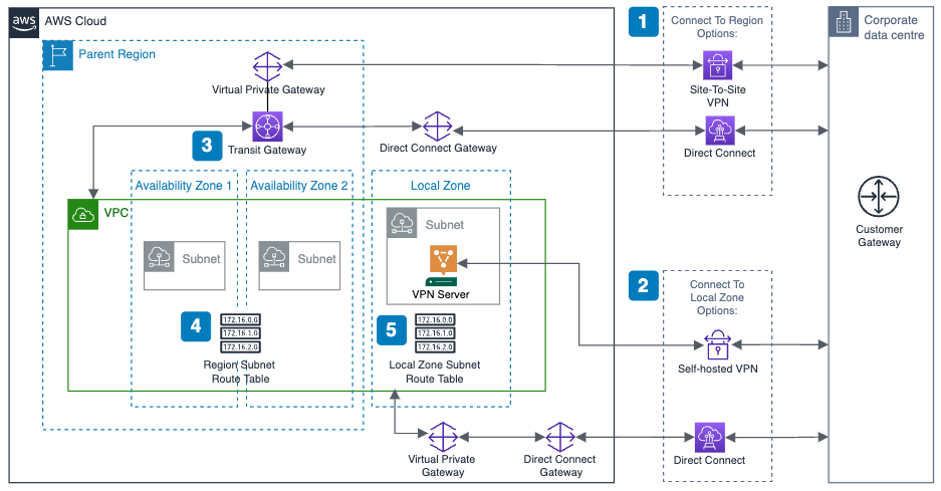
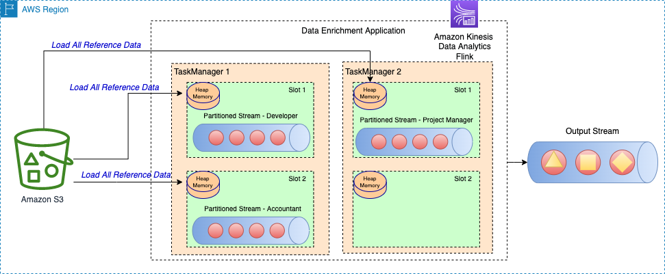
In a soft multi-tenant environment, you can perform chargeback to your data engineering teams based on the resources they consumed and not the nodes allocated. In this method, you use the namespaces associated with the EMR virtual cluster to track how much resources were used for processing jobs. The following diagram illustrates an example.

Diagram -1 Soft multi-tenancy

Tracking resources based on the namespace isn’t an easy task because jobs are transient in nature and fluctuate in their duration. However, there are partner tools available that allow you to keep track of the resources used, such as Kubecost, CloudZero, Vantage, and many others. For instructions on using Kubecost on Amazon EKS, refer to this blog post on cost monitoring for EKS customers.

Sole multi-tenancy

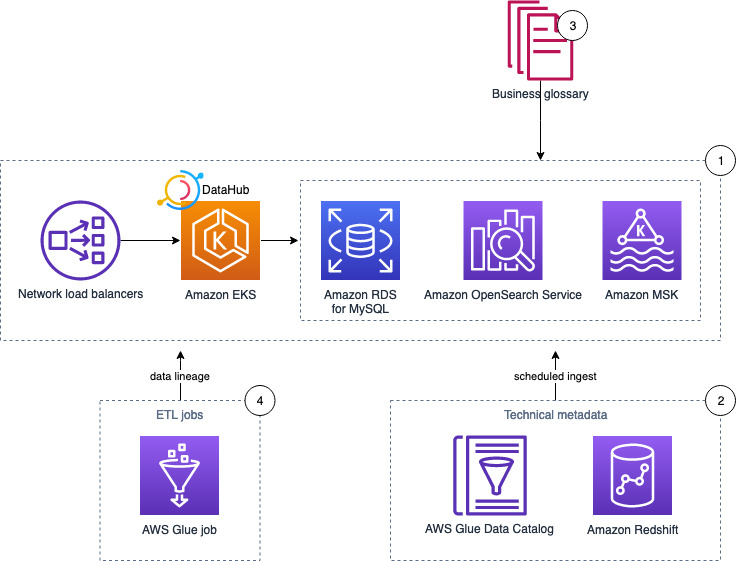
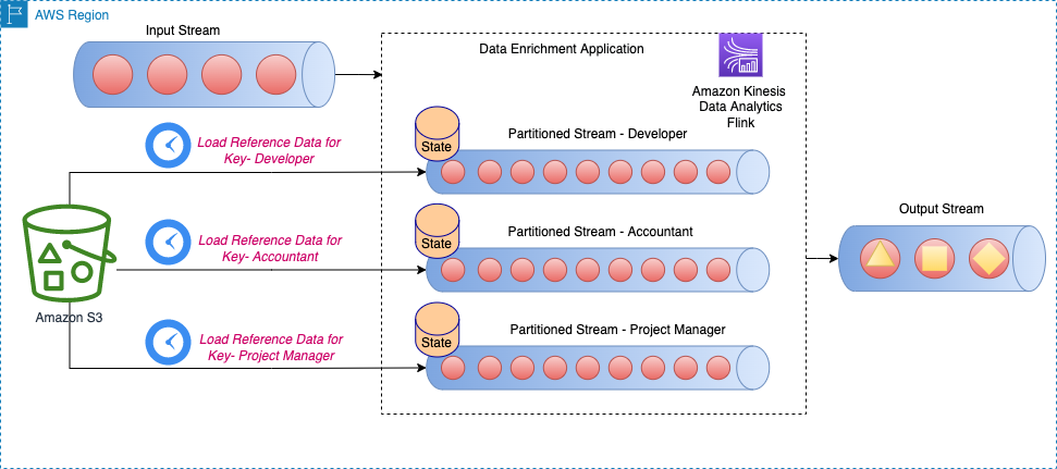
For sole multi-tenancy, the chargeback is done at the instance (node) level. Each member on your team uses a specific set of nodes that are dedicated to it. These nodes aren’t always running, and are spun up using the Kubernetes auto scaling mechanism. The following diagram illustrates an example.

Diagram -2 Sole tenancy

With sole multi-tenancy, you use a cost allocation tag, which is an AWS mechanism that allows you to track how much each resource has consumed. Although the method of sole multi-tenancy isn’t efficient in terms of resource utilization, it provides a simplified strategy for chargebacks. With the cost allocation tag, you can chargeback a team based on all the resources they used, like Amazon S3, Amazon DynamoDB, and other AWS resources. The chargeback mechanism based on the cost allocation tag can be augmented using the recently launched AWS Billing Conductor, which allows you to issue bills internally for your team.

Resource management

In this section, we discuss considerations regarding resource management in multi-tenant clusters. We briefly discuss topics like sharing resources graciously, setting guard rails on resource consumption, techniques for ensuring resources for time sensitive and/or critical jobs, meeting quick resource scaling requirements and finally cost optimization practices with node selectors.

Sharing resources

In a multi-tenant environment, the goal is to share resources like compute and memory for better resource utilization. However, this requires careful capacity management and resource allocation to make sure each tenant gets their fair share. In Kubernetes, resource allocation is controlled and enforced by using ResourceQuota and LimitRange. ResourceQuota limits resources on the namespace level, and LimitRange allows you to make sure that all the containers are submitted with a resource requirement and a limit. In this section, we demonstrate how a data engineer or Kubernetes administrator can set up ResourceQuota as a LimitRange configuration.

The administrator creates one ResourceQuota per namespace that provides constraints for aggregate resource consumption:

apiVersion: v1
kind: ResourceQuota
metadata:
  name: compute-resources
  namespace: teamA
spec:
  hard:
    requests.cpu: "1000"
    requests.memory: 4000Gi
    limits.cpu: "2000"
    limits.memory: 6000Gi

For LimitRange, the administrator can review the following sample configuration. We recommend using default and defaultRequest to enforce the limit and request field on containers. Lastly, from a data engineer perspective while submitting the EMR on EKS jobs, you need to make sure the Spark parameters of resource requirements are within the range of the defined LimitRange. For example, in the following configuration, the request for spark.executor.cores=7 will fail because the max limit for CPU is 6 per container:

apiVersion: v1
kind: LimitRange
metadata:
  name: cpu-min-max
  namespace: teamA
spec:
  limits:
  - max:
      cpu: "6"
    min:
      cpu: "100m"
    default:
      cpu: "500m"
    defaultRequest:
      cpu: "100m"
    type: Container

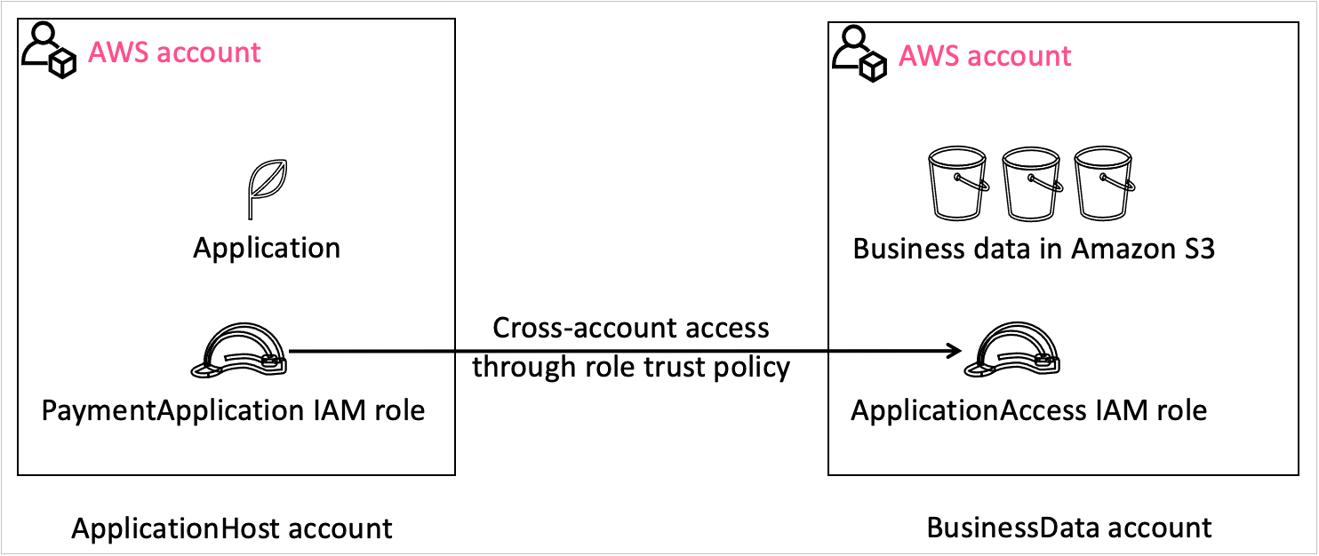
Priority-based resource allocation

Diagram – 3 Illustrates an example of resource allocation with priority.

As all the EMR virtual clusters share the same EKS computing platform with limited resources, there will be scenarios in which you need to prioritize jobs in a sensitive timeline. In this case, high-priority jobs can utilize the resources and finish the job, whereas low-priority jobs that are running gets stopped and any new pods must wait in the queue. EMR on EKS can achieve this with the help of pod templates, where you specify a priority class for the given job.

When a pod priority is enabled, the Kubernetes scheduler orders pending pods by their priority and places them in the scheduling queue. As a result, the higher-priority pod may be scheduled sooner than pods with lower priority if its scheduling requirements are met. If this pod can’t be scheduled, the scheduler continues and tries to schedule other lower-priority pods.

The preemptionPolicy field on the PriorityClass defaults to PreemptLowerPriority, and the pods of that PriorityClass can preempt lower-priority pods. If preemptionPolicy is set to Never, pods of that PriorityClass are non-preempting. In other words, they can’t preempt any other pods. When lower-priority pods are preempted, the victim pods get a grace period to finish their work and exit. If the pod doesn’t exit within that grace period, that pod is stopped by the Kubernetes scheduler. Therefore, there is usually a time gap between the point when the scheduler preempts victim pods and the time that a higher-priority pod is scheduled. If you want to minimize this gap, you can set a deletion grace period of lower-priority pods to zero or a small number. You can do this by setting the terminationGracePeriodSeconds option in the victim Pod YAML.

See the following code samples for priority class:

apiVersion: scheduling.k8s.io/v1
kind: PriorityClass
metadata:
  name: high-priority
value: 100
globalDefault: false
description: " High-priority Pods and for Driver Pods."

apiVersion: scheduling.k8s.io/v1
kind: PriorityClass
metadata:
  name: low-priority
value: 50
globalDefault: false
description: " Low-priority Pods."

One of the key considerations while templatizing the driver pods, especially for low-priority jobs, is to avoid the same low-priority class for both driver and executor. This will save the driver pods from getting evicted and lose the progress of all its executors in a resource congestion scenario. In this low-priority job example, we have used a high-priority class for driver pod templates and low-priority classes only for executor templates. This way, we can ensure the driver pods are safe during the eviction process of low-priority jobs. In this case, only executors will be evicted, and the driver can bring back the evicted executor pods as the resource becomes freed. See the following code:

apiVersion: v1
kind: Pod
spec:
  priorityClassName: "high-priority"
  nodeSelector:
    eks.amazonaws.com/capacityType: ON_DEMAND
  containers:
  - name: spark-kubernetes-driver # This will be interpreted as Spark driver container

apiVersion: v1
kind: Pod
spec:
  priorityClassName: "low-priority"
  nodeSelector:
    eks.amazonaws.com/capacityType: SPOT
  containers:
  - name: spark-kubernetes-executors # This will be interpreted as Spark executor container

Overprovisioning with priority

Diagram – 4 Illustrates an example of overprovisioning with priority.

As pods wait in a pending state due to resource availability, additional capacity can be added to the cluster with Amazon EKS auto scaling. The time it takes to scale the cluster by adding new nodes for deployment has to be considered for time-sensitive jobs. Overprovisioning is an option to mitigate the auto scaling delay using temporary pods with negative priority. These pods occupy space in the cluster. When pods with high priority are unschedulable, the temporary pods are preempted to make the room. This causes the auto scaler to scale out new nodes due to overprovisioning. Be aware that this is a trade-off because it adds higher cost while minimizing scheduling latency. For more information about overprovisioning best practices, refer to Overprovisioning.

Node selectors

EKS clusters can span multiple Availability Zones in a VPC. A Spark application whose driver and executor pods are distributed across multiple Availability Zones can incur inter- Availability Zone data transfer costs. To minimize or eliminate the data transfer cost, you should configure the job to run on a specific Availability Zone or even specific node type with the help of node labels. Amazon EKS places a set of default labels to identify capacity type (On-Demand or Spot Instance), Availability Zone, instance type, and more. In addition, we can use custom labels to meet workload-specific node affinity.

EMR on EKS allows you to choose specific nodes in two ways:

At the job level. Refer to EKS Node Placement for more details.
In the driver and executor level using pod templates.

When using pod templates, we recommend using on demand instances for driver pods. You can also consider including spot instances for executor pods for workloads that are tolerant of occasional periods when the target capacity is not completely available. Leveraging spot instances allow you to save cost for jobs that are not critical and can be terminated. Please refer Define a NodeSelector in PodTemplates.

Conclusion

In this post, we provided guidance on how to design and deploy EMR on EKS in a multi-tenant EKS environment through different lenses: network, security, cost management, and resource management. For any deployment, we recommend the following:

Use IRSA with a condition scoped on the EMR on EKS service account
Use a secret manager to store credentials and the Secret Store CSI Driver to access them in your Spark application
Use ResourceQuota and LimitRange to specify the resources that each of your data engineering teams can use and avoid compute resource abuse and starvation
Implement a network policy to segregate network traffic between pods

Lastly, if you are considering migrating your spark workload to EMR on EKS you can further learn about design patterns to manage Apache Spark workload in EMR on EKS in this blog and about migrating your EMR transient cluster to EMR on EKS in this blog.

About the Authors

Lotfi Mouhib is a Senior Solutions Architect working for the Public Sector team with Amazon Web Services. He helps public sector customers across EMEA realize their ideas, build new services, and innovate for citizens. In his spare time, Lotfi enjoys cycling and running.

Ajeeb Peter is a Senior Solutions Architect with Amazon Web Services based in Charlotte, North Carolina, where he guides global financial services customers to build highly secure, scalable, reliable, and cost-efficient applications on the cloud. He brings over 20 years of technology experience on Software Development, Architecture and Analytics from industries like finance and telecom.

Implementing long running deployments with AWS CloudFormation Custom Resources using AWS Step Functions

2022-09-17 DAMODAR SHENVI WAGLE

Post Syndicated from DAMODAR SHENVI WAGLE original https://aws.amazon.com/blogs/devops/implementing-long-running-deployments-with-aws-cloudformation-custom-resources-using-aws-step-functions/

AWS CloudFormation custom resource provides mechanisms to provision AWS resources that don’t have built-in support from CloudFormation. It lets us write custom provisioning logic for resources that aren’t supported as resource types under CloudFormation. This post focusses on the use cases where CloudFormation custom resource is used to implement a long running task/job. With custom resources, you can manage these custom tasks (which are one-off in nature) as deployment stack resources.

The routine pattern used for implementing custom resources is via AWS Lambda function. However, when using the Lambda function as the custom resource provider, you must consider its trade-offs, such as its 15 minute timeout. Tasks involved in the provisioning of certain AWS resources can be long running and could span beyond the Lambda timeout. In these scenarios, you must look beyond the conventional Lambda function-based approach for custom resources.

In this post, I’ll demonstrate how to use AWS Step Functions to implement custom resources using AWS Cloud Development Kit (AWS CDK). Step Functions allow complex deployment tasks to be orchestrated as a step-by-step workflow. It also offers direct integration with any AWS service via AWS SDK integrations. By default the CloudFormation stack waits for 1 hour before timing out. The timeout can be increased to maximum 12 hours using wait conditions. In this post, you’ll also see how to use wait conditions with custom resource to run long running deployment tasks as part of a CloudFormation stack.

Prerequisites

Before proceeding any further, you must identify and designate an AWS account required for the solution to work. You must also create an AWS account profile in ~/.aws/credentials for the designated AWS account, if you don’t already have one. The profile must have sufficient permissions to run an AWS CDK stack. It should be your private profile and only be used during the course of this post. Therefore, it should be fine if you want to use admin privileges. Don’t share the profile details, especially if it has admin privileges. I recommend removing the profile when you’re finished with this walkthrough. For more information about creating an AWS account profile, see Configuring the AWS CLI.

Services and frameworks used in the post include CloudFormation, Step Functions, Lambda, DynamoDB, Amazon S3, and AWS CDK.

Solution overview

The following architecture diagram shows the application of Step Functions to implement custom resources.

Figure 1. Architecture diagram

The user deploys a CloudFormation stack that includes a custom resource implementation.
The CloudFormation custom resource triggers a Lambda function with the appropriate event which can be CREATE/UPDATE/DELETE.
The custom resource Lambda function invokes Step Functions workflow and offloads the event handling responsibility. The CloudFormation event and context are wrapped inside the Step Function input at the time of invocation.
The custom resource Lambda function returns SUCCESS back to CloudFormation stack indicating that the custom resource provisioning has begun. CloudFormation stack then goes into waiting mode where it waits for a SUCCESS or FAILURE signal to continue.
In the interim, Step Functions workflow handles the custom resource event through one or more steps.
Step Functions workflow prepares the response to be sent back to CloudFormation stack.
Send Response Lambda function sends a success/failure response back to CloudFormation stack. This propels CloudFormation stack out of the waiting mode and into completion.

Solution deep dive

In this section I will get into the details of several key aspects of the solution

Custom Resource Definition

Following code snippet shows the custom resource definition which can be found here. Please note that we also define AWS::CloudFormation::WaitCondition and AWS::CloudFormation::WaitConditionHandle alongside the custom resource. AWS::CloudFormation::WaitConditionHandle resource sets up a pre-signed URL which is passed into the CallbackUrl property of the Custom Resource.

The final completion signal for the custom resource i.e. SUCCESS/FAILURE is received over this CallbackUrl. To learn more about wait conditions please refer to its user guide here. Note that, when updating the custom resource, you cannot use the existing WaitCondition-WaitConditionHandle resource pair. You need to create a new pair for tracking each update/delete operation on the custom resource.

/************************** Custom Resource Definition *****************************/
// When you intend to update CustomResource make sure that a new WaitCondition and 
// a new WaitConditionHandle resource is created to track CustomResource update.
// The strategy we are using here is to create a hash of Custom Resource properties.
// The resource names for WaitCondition and WaitConditionHandle carry this hash.
// Anytime there is an update to the custom resource properties, a new hash is generated,
// which automatically leads to new WaitCondition and WaitConditionHandle resources.
const resourceName: string = getNormalizedResourceName('DemoCustomResource');
const demoData = {
    pk: 'demo-sfn',
    sk: resourceName,
    ts: Date.now().toString()
};
const dataHash = hash(demoData);
const wcHandle = new CfnWaitConditionHandle(
    this, 
    'WCHandle'.concat(dataHash)
)
const customResource = new CustomResource(this, resourceName, {
    serviceToken: customResourceLambda.functionArn,
    properties: {
        DDBTable: String(demoTable.tableName),
        Data: JSON.stringify(demoData),
        CallbackUrl: wcHandle.ref
    }
});
        
// Note: AWS::CloudFormation::WaitCondition resource type does not support updates.
new CfnWaitCondition(
    this,
    'WC'.concat(dataHash),
    {
        count: 1,
        timeout: '300',
        handle: wcHandle.ref
    }
).node.addDependency(customResource)
/**************************************************************************************/

Custom Resource Lambda

Following code snippet shows how the custom resource lambda function passes the CloudFormation event as an input into the StepFunction at the time of invocation. CloudFormation event contains the CallbackUrl resource property I discussed in the previous section.

private async startExecution() {
    const input = {
        cfnEvent: this.event,
        cfnContext: this.context
    };
    const params: StartExecutionInput = {
        stateMachineArn: String(process.env.SFN_ARN),
        input: JSON.stringify(input)
    };
    let attempt = 0;
    let retry = false;
    do {
        try {
            const response = await this.sfnClient.startExecution(params).promise();
            console.debug('Response: ' + JSON.stringify(response));
            retry = false;

Custom Resource StepFunction

The StepFunction handles the CloudFormation event based on the event type. The CloudFormation event containing CallbackUrl is passed down the stages of StepFunction all the way to the final step. The last step of the StepFunction sends back the response over CallbackUrl via send-cfn-response lambda function as shown in the following code snippet.

/**
 * Send response back to cloudformation
 * @param event
 * @param context
 * @param response
 */
export async function sendResponse(event: any, context: any, response: any) {
    const responseBody = JSON.stringify({
        Status: response.Status,
        Reason: "Success",
        UniqueId: response.PhysicalResourceId,
        Data: JSON.stringify(response.Data)
    });
    console.debug("Response body:\n", responseBody);
    const parsedUrl = url.parse(event.ResourceProperties.CallbackUrl);
    const options = {
        hostname: parsedUrl.hostname,
        port: 443,
        path: parsedUrl.path,
        method: "PUT",
        headers: {
            "content-type": "",
            "content-length": responseBody.length
        }
    };
    await new Promise(() => {
        const request = https.request(options, function(response: any) {
	    console.debug("Status code: " + response.statusCode);
	    console.debug("Status message: " + response.statusMessage);
	    context.done();
    	})
	request.on("error", function(error) {
	    console.debug("send(..) failed executing https.request(..): " + error);
	    context.done();
	});
	request.write(responseBody);
	request.end();
    });
    return;
}

Demo

Clone the GitHub repo cfn-custom-resource-using-step-functions and navigate to the folder cfn-custom-resource-using-step-functions. Now, execute the script script-deploy.sh by passing the name of the AWS profile that you created in the prerequisites section above. This should deploy the solution. The commands are shown as follows for your reference. Note that if you don’t pass the AWS profile name ‘default’ the profile will be used for deployment.

git clone 
cd cfn-custom-resource-using-step-functions
./script-deploy.sh "<AWS- ACCOUNT-PROFILE-NAME>"

The deployed solution consists of 2 stacks as shown in the following screenshot

cfn-custom-resource-common-lib: Deploys common components
- DynamoDB table that custom resources write to during their lifecycle events
- Lambda layer used across the rest of the stacks
cfn-custom-resource-sfn: Deploys Step Functions backed custom resource implementation

Figure 2. CloudFormation stacks deployed

For demo purposes, I implemented a custom resource that inserts data into the DynamoDB table. When you deploy the solution for the first time, like you just did in the previous step, it initiates a CREATE event resulting in the creation of a new custom resource using Step Functions. You should see a new record with unix epoch timestamp in the DynamoDB table, indicating that the resource was created as shown in the following screenshot. You can find the DynamoDB table name/arn from the SSM Parameter Store /CUSTOM_RESOURCE_PATTERNS/DYNAMODB/ARN

Figure 3. DynamoDB record indicating custom resource creation

Now, execute the script script-deploy.sh again. This should initiate an UPDATE event, resulting in the update of custom resources. The code also automatically creates new WaitConditionHandle and WaitCondition resources required to wait for the update event to finish. Now you should see that the records in the DynamoDb table have been updated with new values for lastOperation and ts attributes as follows.

Figure 4. DynamoDB record indicating custom resource update

Cleaning up

To remove all of the stacks, run the script script-undeploy.sh as follows.

./script-undeploy.sh "<AWS- ACCOUNT-PROFILE-NAME>"

Conclusion

In this post I showed how to look beyond the conventional approach of building CloudFormation custom resources using a Lambda function. I discussed implementing custom resources using Step Functions and CloudFormation wait conditions. Try this solution in scenarios where you must execute a long running deployment task/job as part of your CloudFormation stack deployment.

About the author:

Hazard analysis and Chaos engineering at Vanguard Group

2022-09-16 Jason Barto

Post Syndicated from Jason Barto original https://aws.amazon.com/blogs/devops/hazard-analysis-and-chaos-engineering-at-vanguard-group/

Anticipating events that can cause a disruption to your system’s service is critical to building highly available, reliable systems. Hazard analysis gives you a method to identify such events. Chaos engineering gives you a method to confirm that a system behaves as expected in adverse conditions. By combining these methods, Vanguard is building reliability into their systems.

Vanguard engineering teams perform hazard analysis on their systems and capture the identified events as failure scenarios. They use the identified failure scenarios to create hypotheses to support chaos engineering experiments. These hypotheses predict how the system will respond to failures and each hypothesis is then confirmed through experimentation to increase the team’s confidence in the system’s reliability.

In this article we will walk you through how Vanguard uses hazard analysis and chaos engineering. We will also provide guidance on how you can employ these techniques on your applications.

Failure Mode & Effects Analysis

A hazard analysis can be performed using different methods. At Vanguard, they have adapted the failure mode & effects analysis (FMEA) method to support their important services.

FMEA is a bottom-up approach to analyse an architecture and focus on the impact to system functions when one or more components of the system are disrupted. Members of the engineering team and architects responsible for designing and building a system brainstorm possible failure scenarios or failure modes, and document the impact of these failures on the system. Combined with a quantitative method for ranking the failure modes, the analysis process produces a prioritised list of failure modes which describes how the system would respond to individual or combined failures in its component parts or dependencies.

For each failure mode the team conducting the analysis will highlight what protections exist within the system to guard against the failure mode. Sometimes, fault isolation boundaries have been put in place to prevent client impact in failure scenarios. In other scenarios, for one reason or another, there are hard dependencies in place for which the engineering team has decided not to build in fault tolerance. For example, a team responsible for a less-critical function may have architected its system to operate across multiple availability zones, but could decide not to implement other mitigations to prioritize cost over increased resilience.

The FMEA method has been in use by engineers in the automotive, aeronautical, healthcare, and military industries for more than 60 years. Over that time, FMEA has been modified to best suit the organization and the field in which it was applied. In many variations the FMEA measures each failure mode with a risk priority number (RPN), which is intended to quantitatively rank the failure mode based upon:

The failure mode’s impact to the system as a whole
The probability of the failure mode’s occurrence
How easily the failure mode can be detected

Vanguard have adapted the FMEA process to serve their own specific requirements and processes. Vanguard have decided not to adopt the RPN element of the FMEA process, as teams found they spent a lot of time debating the impact, probability, and detectability of individual failure modes. To perform an FMEA more quickly, teams instead focus on the failure modes and system impact only, documenting a mental model of system performance which can be experimented through chaos engineering.

An excerpt of a Vanguard FMEA output is provided as an example in the following table:

The “Process Step” in the table above refers to a business function of the system being analyzed, for example “Request to retrieve stored data”. As part of the analysis, the team identifies the system components needed to perform the Process Step and considers the interactions of those components Focusing on a Process Step makes it easier to anticipate the failure scenarios that would affect the system in performing this particular business function. Also, the Process Step will imply an importance or criticality which can be a factor when prioritizing mitigations.

After selecting a Process Step, you walk through the system components involved and identify how component failures or disruptions will affect the wider system. Such component failures may involve individual components or a combination of components and are captured as “Failure Mode”. This identifies the component or components that are disrupted and their behaviour; for example, “Microservice is unavailable or returns an error”.

“Expected Behaviour” describes the effect of the failure mode on the wider system, in the context of the Process Step. This captures what other system components are affected by the Failure Mode and why, and how this impacts the Process Step as a whole.

Lastly, the “Hypothesis” column forms the basis for the chaos experiments that will follow from the FMEA to confirm that the system performs as expected.

At Vanguard, all mission-critical product teams are conducting FMEAs for their production applications. The outputs of these sessions are maintained over time and serve multiple purposes:

When onboarding new team members, it is helpful to provide the FMEA document alongside an architecture diagram and narrative. It will paint a more robust picture of how the system is intended to operate in both “happy path” and “unhappy path” scenarios.
When troubleshooting incidents, an FMEA document can help on-call engineers – especially those less experienced with debugging – to match up the documented expectations to the observed system behavior.
Site Reliability Engineers (SREs) looking for opportunities to improve the resilience of a system might look to FMEA documentation to understand the existing fault isolation boundaries and introduce additional resilience mechanisms through automation and system changes.
Finally, when selecting scenarios for experimentation with Chaos Engineering, the FMEA document provides a list of conjectures that have been mapped to hypotheses, ready to be validated through experimentation. This input into the Chaos Engineering workflow is the primary use of FMEA documents for Vanguard product teams.

There are many resources available online to learn more about how FMEA is used and applied in other organisations. In Failure Modes and Continuous Resilience, Adrian Cockcroft introduces FMEA as a method for anticipating failure scenarios. The NASA Software Engineering Handbook details how FMEAs are conducted as part of their engineering process. The Automotive Industry Group has also formally documented the use of FMEA in the Automotive Industry Action Group FMEA Handbook.

Chaos Engineering

After failure modes have been identified and mitigated through system design, it’s time to understand how resilient the system’s implementation is to those failure modes. Chaos engineering can be used to explore a system and validate that a system’s implementation meets business resiliency objectives.

Chaos engineering helps to improve a team’s mental model about the system under experimentation and provides insights into how a complex system behaves under adverse conditions. It also enables an engineer to find the unknown unknowns and the known unknowns through experiments that are built on top of the hypothesis. These experiments should simulate real world events, such as network degradation and increased client requests, and the outcome of the experiment should not be known. In other words, an experiment is not an experiment if it’s known that the conditions will cause the system to fail.

Prerequisites to Chaos Experiments at Vanguard

At Vanguard, there are some necessary prerequisites to running a chaos experiment. Firstly, the system under experiment must be set up with some basic observability tooling that will allow teams to monitor the state of the application during the failure injection. This could be as simple as an Amazon CloudWatch dashboard and some associated alarms, or as elaborate as a dedicated dashboard set up in a vendor tool.

Secondly, teams must be able to drive load to the application during the experiment; depending on the experiment type, the level and type of load may vary. The load generator can be as simple as a script on someone’s machine, or a fully automated load test depending on the requirements of the hypothesis.

Finally, teams need to have a good understanding of what the application’s “steady state” looks like. I Ideally, this takes the form of some metrics such as expected error rate, expected latency, and/or a service level objective (SLO) that can be monitored throughout the duration of the experiment. For example, a service level objective for a RESTful API might be that 90% of requests should receive a response within 100 milliseconds.

With the prerequisites met and a completed FMEA, teams can then experiment with their hypothesis using various experiment templates defined by Vanguard’s Climate of Chaos tooling.

Vanguard’s Climate of Chaos

At Vanguard, ensuring its software systems are resilient to adverse events is a critical part of its ongoing mission to provide world-class service to their clients. Vanguard believes that in order to develop high quality software, one must plan for the inevitable “stormy weather” events that occur in a distributed system.

Over the past 2 years, as a response to this need, Vanguard has developed in-house tooling called “The Climate of Chaos” to give teams easy access to common experiment templates, along with a friendly UI interface. The Climate of Chaos helps developers experiment on their systems and validate the hypotheses generated from FMEAs. It also provides the tooling for them to simulate the most common failure scenarios on Vanguard’s most commonly utilized AWS infrastructure, including Amazon Elastic Container Service (Amazon ECS), AWS Fargate, Amazon DynamoDB, Amazon Relational Database Service (Amazon RDS), AWS Lambda, and others.

The Climate of Chaos was created prior to Amazon’s release of the AWS Fault Injection Simulator (FIS), and today there is a lot of overlap with the experiment capabilities available in FIS. The Climate of Chaos has also been enhanced with company-specific features and integrations that make it easier for Vanguard developers to run chaos experiments in a controlled and predictable manner.

The Climate of Chaos includes important safety features such as an “emergency stop” function. This feature enables teams to terminate the experiment immediately if unintended side effects are encountered, rolling back the events simulated to resume steady state operation. The Climate of Chaos has been coupled with other systems like an in-house load testing tooling and added features like the ability to monitor CloudWatch alarms. Vanguard also offers teams the ability to schedule experiments to run at their convenience. Soon, Vanguard hopes to make running chaos experiments even smarter, introducing tools that will help teams run bulk experiments that systematically inject failures on a group of related applications to help pinpoint more complex failure modes.

Next Steps

Failure modes and effects analysis is a hazard analysis method which can help you identify single and combined points of failure in your system so you can prioritize the failure modes. To learn more about the FMEA process, you can read the NASA Software Engineering Handbook which outlines how they perform FMEA on their software-based systems. The AWS Whitepaper Building Mission-Critical Financial Services Applications on AWS provides example forms and suggestions for severity, probability, and detectability rankings. Appendix F in the whitepaper suggests a 1 to 10 ranking for each Risk Priority Number input, and the example spreadsheets recommend performing FMEAs for the application, platform, infrastructure, and operation layers of the system. Using these examples, you can perform an analysis of your own systems and generate hypotheses.

To experiment on your systems and validate your own hypotheses, you can use the AWS Fault Injection Simulator (FIS) mentioned earlier in this article. FIS provides you with a framework for performing controlled chaos experiments on your AWS workloads. It helps you to safely manage your experiments by providing tooling to monitor, rollback, and orchestrate chaos experiments. FIS provides the fault injection mechanisms that you will need to experiment upon your system’s implementation and resilience to identified failure modes. You can start by running experiments in pre-production environments, and then step up to running them as part of your CI/CD workflow and ultimately in your production environment. To learn more about FIS, you can read the FIS User Guide and FIS tutorials.

By using FMEA to anticipate the failures and experimenting on your systems with chaos engineering, you will gain confidence in the reliability of your system.

The content and opinions in this post are those of The Vanguard Group and AWS is not responsible for the content or accuracy of this post.

About the authors:

Deploying Local Gateway Ingress Routing on AWS Outposts

2022-09-15 Sheila Busser

Post Syndicated from Sheila Busser original https://aws.amazon.com/blogs/compute/deploying-local-gateway-ingress-routing-on-aws-outposts/

This post is written by Leonardo Solano, Senior Hybrid Cloud Solution Architect and Chris Lunsford, Senior Specialist Solutions Architect, AWS Outposts.

AWS Outposts lets customers use the same Amazon Virtual Private Cloud (VPC) security mechanisms, such as security groups and network access control lists, to control traffic flows for on-premises applications running on Outposts. Some customers, desiring additional security or consistency with on-premises systems, want the ability to inspect and filter incoming application traffic as it enters the Outpost. Ideally, they would like to deploy virtual appliances in front of the workloads running on Outposts.

Today, we are announcing a new feature called Outposts local lateway (LGW) ingress routing. This lets you create LGW inbound routes to redirect incoming traffic to an Amazon Elastic Compute Cloud (EC2) Elastic Network Interface (ENI) associated with an EC2 instance running on Outposts rack. The traffic is redirected for inspection before it reaches the workloads running on Outposts rack. Moreover, it lets the EC2 virtual appliance inspect, filter, or optimize the traffic in a similar way as VPC ingress routing in the Region.

Use case

A common use case for this feature is deploying a customer-preferred third-party virtual network appliance. The appliance can inspect, modify, or monitor the incoming traffic for policy compliance and forward compliant traffic on to the workloads running on the Outpost. A typical virtual appliance could be a firewall, intrusion detection system (IDS), or intrusion prevention system (IPS). The features provided by the virtual appliances vary, and they may include deep packet inspection, traffic optimization, and flow monitoring. This new Outposts rack feature modifies the default behavior of the local gateway routing table (LGW-RTB), and it lets customers redirect traffic coming into an Outposts deployment to the virtual appliance.

The new behavior?

Now you can create static routes in the LGW-RTB that target a specific ENI on the Outpost as the next hop. These static routes are propagated toward the customer network through the Border Gateway Protocol (BGP) peering sessions with the Customer Networking Devices. The on-premises network will route traffic to the specified Classless Inter-Domain Routing (CIDR) prefixes, as defined in the static routes, toward the Outposts Network Devices.

In the preceeding diagram, the static route 198.19.33.248/29 has a longer prefix length than 198.19.33.240/28, and both routes will be propagated toward the customer network via BGP. The incoming traffic for the 198.19.33.248/29 prefix will be directed toward the ENI eni-1234example0. The architecture looks like the following diagram, where the security virtual appliance is seated between the LGW and a set of EC2 instances in Outposts.

As ingress traffic is routed through the virtual appliance for inspection and filtering, the destination addresses of packets arriving at the ENI of the virtual appliance won’t match its ENI’s private IP address (the packets are transiting the instance). By default, the ENI will drop the inbound traffic unless you disable source/destination checking on the virtual appliance instance ENI settings. The following screenshot shows how you can disable the EC2 instance source/destination checking in the AWS console.

Considerations for LGW ingress routing

Consider the following requirements when preparing to deploy LGW ingress routing:

The ENIs used as the next-hop target must be deployed in an Outposts Subnet.
The subnets must belong to a VPC associated with the LGW-RTB.
Routes with the longest matches are prioritized. If there are two with the same destination CIDR, then static routes are preferred over propagated ones.

Working with Outposts LGW ingress routing

The following output shows what the LGW route table looks like before applying the ingress routing feature:

{
    "Routes": [
        {
            "DestinationCidrBlock": "0.0.0.0/0",
            "LocalGatewayVirtualInterfaceGroupId": "lgw-vif-grp-XXX",
            "Type": "static",
            "State": "active",
            "LocalGatewayRouteTableId": "lgw-rtb-XXX",
            "LocalGatewayRouteTableArn": "arn:aws:ec2:>AWS-REGION>:<account-id>:local-gateway-route-table/lgw-rtb-XXX",
            "OwnerId": "<account-id>"
        },
        {
            "DestinationCidrBlock": "198.19.33.16/28",
            "CoipPoolId": "coip-pool-0000aaaabbbbcccc1111",
            "Type": "propagated",
            "State": "active",
            "LocalGatewayRouteTableId": "lgw-rtb-XXX",
            "LocalGatewayRouteTableArn": "arn:aws:ec2:<AWS-REGION>:<account-id>:local-gateway-route-table/lgw-XXX",
            "OwnerId": "<account-id>"
        },
        {
            "DestinationCidrBlock": "198.19.33.240/28",
            "CoipPoolId": "coip-pool-0000aaaabbbbcccc2222",
            "Type": "propagated",
            "State": "active",
            "LocalGatewayRouteTableId": "lgw-rtb-XXX",
            "LocalGatewayRouteTableArn": "arn:aws:ec2:<AWS-REGION>:<account-id>:local-gateway-route-table/lgw-XXX",
            "OwnerId": "<account-id>"
        }
     ]
}

The relevant change under an LGW-RTB before to add a local-gateway-route is the presence of the “propagated routes”. This represents the Outposts Subnets that can’t be deleted or modified with Next-Hop as specific ENIs present in Outposts. In the following section, we will cover how it will look after the creation of a local-gateway-route.

Configuring LGW ingress routing

To configure LGW ingress routing, you must provide the LGW route table ID, the ENI ID that will be utilized as a next-hop, and the destination CIDR block. Once you have identified those three parameters, you can configure LGW ingress routing via the This is shown in the following example, where the prefix 198.19.33.248/29 is routed to an Outpost. If the route points to an ENI attached to an instance, then the route will show as active. If the route points to an ENI that isn’t attached to an EC2 instance, then the route will show a blackhole state.

$ aws ec2 create-local-gateway-route \
  --local-gateway-route-table-id <lgw-rtb-id> \
  --network-interface-id <eni-id> \
  --destination-cidr-block 198.19.33.248/29
  
{
    "Route": {
        "DestinationCidrBlock": "198.19.33.248/29",
        "NetworkInterfaceId": "eni-id",
        "Type": "static",
        "State": "active",
        "LocalGatewayRouteTableId": "lgw-rtb-id",
        "LocalGatewayRouteTableArn": "arn:aws:ec2:<AWS-REGION>:<account-id>:local-gateway-route-table/<lgw-rtb-id>",
        "OwnerId": "<account-id>"
    }
}

Once LGW ingress routing has been configured, the LGW will route traffic destined to the 198.19.33.248/29 prefix to the target ENI. This must be present as part of the Outposts subnets. Note that the segment 198.19.33.248/29 is part of the Outposts CIDR range of 198.19.33.240/28. This belongs, in this case, to the Outposts customer-owned IP address (CoIP) CIDRs. When traffic follows a static route to an ENI, the packet destination address is preserved and isn’t translated to the private address of the ENI.

In this case, the new LGW-RTB will look like the following:

{
    "Routes": [
        {
            "DestinationCidrBlock": "0.0.0.0/0",
            "LocalGatewayVirtualInterfaceGroupId": "lgw-vif-grp-XXX",
            "Type": "static",
            "State": "active",
            "LocalGatewayRouteTableId": "lgw-rtb-XXX",
            "LocalGatewayRouteTableArn": "arn:aws:ec2:<AWS-REGION>:<account-id>:local-gateway-route-table/lgw-rtb-XXX",
            "OwnerId": "<account-id>"
        },
        {
            "DestinationCidrBlock": "198.19.33.16/28",
            "CoipPoolId": "coip-pool-0000aaaabbbbcccc1111",
            "Type": "propagated",
            "State": "active",
            "LocalGatewayRouteTableId": "lgw-rtb-XXX",
            "LocalGatewayRouteTableArn": "arn:aws:ec2:<AWS-REGION>:<account-id>:local-gateway-route-table/lgw-XXX",
            "OwnerId": "<account-id>"
        },
        {
            "DestinationCidrBlock": "198.19.33.240/28",
            "CoipPoolId": "coip-pool-0000aaaabbbbcccc1111",
            "Type": "propagated",
            "State": "active",
            "LocalGatewayRouteTableId": "lgw-rtb-XXX",
            "LocalGatewayRouteTableArn": "arn:aws:ec2:<AWS-REGION>:<account-id>:local-gateway-route-table/lgw-XXX",
            "OwnerId": "<account-id>"
        },
         {
            "DestinationCidrBlock": "198.19.33.248/29",
            "NetworkInterfaceId": "eni-XXX",
            "Type": "static",
            "State": "active",
            "LocalGatewayRouteTableId": "lgw-rtb-XXX",
            "LocalGatewayRouteTableArn": "arn:aws:ec2:<AWS-REGION>:<account-id>:local-gateway-route-table/lgw-rtb-XXX",
            "OwnerId": "<account-id>"
        }
     ]
}

In the AWS console, the LGW-RTB will show the new ingress routing route:

Modifying LGW ingress routing

Utilize a similar AWS CLI command to the one that we used previously to create the LGW ingress routing route to modify existing routes. In this case, the command will be aws ec2 modify-local-gateway-route, and the arguments are the same as with the create command. Use this command when you want to shift inbound traffic from one EC2 instance to another – perhaps from an active to a standby network appliance while you perform required maintenance on the primary instance.

$ aws ec2 modify-local-gateway-route \
  --local-gateway-route-table-id <lgw-rtb-id> \
  --network-interface-id <new-eni-id> \
  --destination-cidr-block 198.19.33.248/29
{
    "Route": {
        "DestinationCidrBlock": "198.19.33.248/29",
        "NetworkInterfaceId": "new-eni-id",
        "Type": "static",
        "State": "active",
        "LocalGatewayRouteTableId": "lgw-rtb-id",
        "LocalGatewayRouteTableArn": "arn:aws:ec2:<AWS-REGION>:<account-id>:local-gateway-route-table/<lgw-rtb-id>",
        "OwnerId": "<account-id>"
    }
}

Conclusion

AWS Outposts LGW ingress routing allows AWS customers and partners to deploy virtual appliances on Outposts rack and direct inbound traffic through those appliances. The virtual appliance can inspect, filter, and optimize the ingress traffic before forwarding it on to the workloads running on Outposts rack, creating fine-grained network and security policies for your workloads. To learn more about AWS Outposts rack, visit the product overview page.