Tag Archives: Best practices

Analyze Amazon Cognito advanced security intelligence to improve visibility and protection

Post Syndicated from Diana Alvarado original https://aws.amazon.com/blogs/security/analyze-amazon-cognito-advanced-security-intelligence-to-improve-visibility-and-protection/

As your organization looks to improve your security posture and practices, early detection and prevention of unauthorized activity quickly becomes one of your main priorities. The behaviors associated with unauthorized activity commonly follow patterns that you can analyze in order to create specific mitigations or feed data into your security monitoring systems.

This post shows you how you can analyze security intelligence from Amazon Cognito advanced security features logs by using AWS native services. You can use the intelligence data provided by the logs to increase your visibility into sign-in and sign-up activities from users, this can help you with monitoring, decision making, and to feed other security services in your organization, such as a web application firewall or security information and event management (SIEM) tool. The data can also enrich available security feeds like fraud detection systems, increasing protection for the workloads that you run on AWS.

Amazon Cognito advanced security features overview

Amazon Cognito provides authentication, authorization, and user management for your web and mobile apps. Your users can sign in to apps directly with a user name and password, or through a third party such as social providers or standard enterprise providers through SAML 2.0/OpenID Connect (OIDC). Amazon Cognito includes additional protections for users that you manage in Amazon Cognito user pools. In particular, Amazon Cognito can add risk-based adaptive authentication and also flag the use of compromised credentials. For more information, see Checking for compromised credentials in the Amazon Cognito Developer Guide.

With adaptive authentication, Amazon Cognito examines each user pool sign-in attempt and generates a risk score for how likely the sign-in request is from an unauthorized user. Amazon Cognito examines a number of factors, including whether the user has used the same device before or has signed in from the same location or IP address. A detected risk is rated as low, medium, or high, and you can determine what actions should be taken at each risk level. You can choose to allow or block the request, require a second authentication factor, or notify the user of the risk by email. Security teams and administrators can also submit feedback on the risk through the API, and users can submit feedback by using a link that is sent to the user’s email. This feedback can improve the risk calculation for future attempts.

To add advanced security features to your existing Amazon Cognito configuration, you can get started by using the steps for Adding advanced security to a user pool in the Amazon Cognito Developer Guide. Note that there is an additional charge for advanced security features, as described on our pricing page. These features are applicable only to native Amazon Cognito users; they aren’t applicable to federated users who sign in with an external provider.

Solution architecture

Figure 1: Solution architecture

Figure 1: Solution architecture

Figure 1 shows the high-level architecture for the advanced security solution. When an Amazon Cognito sign-in event is recorded by AWS CloudTrail, the solution uses an Amazon EventBridge rule to send the event to an Amazon Simple Queue Service (Amazon SQS) queue and batch it, to then be processed by an AWS Lambda function. The Lambda function uses the event information to pull the sign-in security information and send it as logs to an Amazon Simple Storage Service (Amazon S3) bucket and Amazon CloudWatch Logs.

Prerequisites and considerations for this solution

This solution assumes that you are using Amazon Cognito with advanced security features already enabled, the solution does not create a user pool and does not activate the advanced security features on an existing one.

The following list describes some limitations that you should be aware of for this solution:

  1. This solution does not apply to events in the hosted UI, but the same architecture can be adapted for that environment, with some changes to the events processor.
  2. The Amazon Cognito advanced security features support only native users. This solution is not applicable to federated users.
  3. The admin API used in this solution has a default rate limit of 30 requests per second (RPS). If you have a higher rate of authentication attempts, this API call might be throttled and you will need to implement a re-try pattern to confirm that your requests are processed.

Implement the solution

You can deploy the solution automatically by using the following AWS CloudFormation template.

Choose the following Launch Stack button to launch a CloudFormation stack in your account and deploy the solution.

Select this image to open a link that starts building the CloudFormation stack

You’ll be redirected to the CloudFormation service in the US East (N. Virginia) Region, which is the default AWS Region, to deploy this solution. You can change the Region to align it to where your Cognito User Pool is running.

This template will create multiple cloud resources including, but not limited to, the following:

  • An EventBridge rule for sending the Amazon Cognito events
  • An Amazon SQS queue for sending the events to Lambda
  • A Lambda function for getting the advanced security information based on the authentication events from CloudTrail
  • An S3 bucket to store the logs

In the wizard, you’ll be asked to modify or provide one parameter, the existing Cognito user pool ID. You can get this value from the Amazon Cognito console or the Cognito API.

Now, let’s break down each component of the solution in detail.

Sending the authentication events from CloudTrail to Lambda

Cognito advanced security features supports the CloudTrail events: SignUp, ConfirmSignUp, ForgotPassword, ResendConfirmationCode, InitiateAuth and RespondToAuthChallenge. This solution will focus on the sign-in event InitiateAuth as an example.

The solution creates an EventBridge rule that will run when an event is identified in CloudTrail and send the event to an SQS queue. This is useful so that events can be batched up and decoupled for Lambda to process.

The EventBridge rule uses Amazon SQS as a target. The queue is created by the solution and uses the default settings, with the exception that Receive message wait time is set to 20 seconds for long polling. For more information about long polling and how to manually set up an SQS queue, see Consuming messages using long polling in the Amazon SQS Developer Guide.

When the SQS queue receives the messages from EventBridge, these are sent to Lambda for processing. Let’s now focus on understanding how this information is processed by the Lambda function.

Using Lambda to process Amazon Cognito advanced security features information

In order to get the advanced security features evaluation information, you need authentication details that can only be obtained by using the Amazon Cognito identity provider (IdP) API call admin_list_user_auth_events. This API call requires a username to fetch all the authentication event details for a specific user. For security reasons, the username is not logged in CloudTrail and must be obtained by using other event information.

You can use the Lambda function in the sample solution to get this information. It’s composed of three main sequential actions:

  1. The Lambda function gets the sub identifiers from the authentication events recorded by CloudTrail.
  2. Each sub identifier is used to get the user name through an API call to list_users.
  3. 3. The sample function retrieves the last five authentication event details from advanced security features for each of these users by using the admin_list_user_auth_events API call. You can modify the function to retrieve a different number of events, or use other criteria such as a timestamp or a specific time period.

Getting the user name information from a CloudTrail event

The following sample authentication event shows a sub identifier in the CloudTrail event information, shown as sub under additionalEventData. With this sub identifier, you can use the ListUsers API call from the Cognito IdP SDK to get the user name details.

{
"eventVersion": "1.XX",
"userIdentity": {
"type": "Unknown",
"principalId": "Anonymous"
},
"eventTime": "2022-01-01T11:11:11Z",
"eventSource": "cognito-idp.amazonaws.com",
"eventName": "InitiateAuth",
"awsRegion": "us-east-1",
"sourceIPAddress": "xx.xx.xx.xx",
"userAgent": "Mozilla/5.0 (xxxx)",
"requestParameters": {
"authFlow": "USER_SRP_AUTH",
"authParameters": "HIDDEN_DUE_TO_SECURITY_REASONS",
"clientMetadata": {},
"clientId": "iiiiiiiii"
},
"responseElements": {
"challengeName": "PASSWORD_VERIFIER",
"challengeParameters": {
"SALT": "HIDDEN_DUE_TO_SECURITY_REASONS",
"SECRET_BLOCK": "HIDDEN_DUE_TO_SECURITY_REASONS",
"USER_ID_FOR_SRP": "HIDDEN_DUE_TO_SECURITY_REASONS",
"USERNAME": "HIDDEN_DUE_TO_SECURITY_REASONS",
"SRP_B": "HIDDEN_DUE_TO_SECURITY_REASONS"
}
},
"additionalEventData": {
"sub": "11110b4c-1f4264cd111"
},
"requestID": "xxxxxxxx",
"eventID": "xxxxxxxxxx",
"readOnly": false,
"eventType": "AwsApiCall",
"managementEvent": true,
"recipientAccountId": "xxxxxxxxxxxxx",
"eventCategory": "Management"
}

Listing authentication events information

After the Lambda function obtains the username, it can then use the Cognito IdP API call admin_list_user_auth_events to get the advanced security feature risk evaluation information for each of the authentication events for that user. Let’s look into the details of that evaluation.

The authentication event information from Amazon Cognito advanced security provides information for each of the categories evaluated and logs the results. Those results can then be used to decide whether the authentication attempt information is useful for the security team to be notified or take action. It’s recommended that you limit the number of events returned, in order to keep performance optimized.

The following sample event shows some of the risk information provided by advanced security features; the options for the response syntax can be found in the CognitoIdentityProvider API documentation.

}
]
at the bottom, so
"AuthEvents": [
{
"EventId": "1111111”,
"EventType": "SignIn",
"CreationDate": 111111.111,
"EventResponse": "Pass",
"EventRisk": {
"RiskDecision": "NoRisk",
"CompromisedCredentialsDetected": false
},
"ChallengeResponses": [
{
"ChallengeName": "Password",
"ChallengeResponse": "Success"
}
],
"EventContextData": {
"IpAddress": "72.xx.xx.xx",
"DeviceName": "Firefox xx
"City": "Axxx",
"Country": "United States"
}
}
]

The event information that is returned includes the details that are highlighted in this sample event, such as CompromisedCredentialsDetected, RiskDecision, and RiskLevel, which you can evaluate to decide whether the information can be used to enrich other security monitoring services.

Logging the authentication events information

You can use a Lambda extensions layer to send logs to an S3 bucket. Lambda still sends logs to Amazon CloudWatch Logs, but you can disable this activity by removing the required permissions to CloudWatch on the Lambda execution role. For more details on how to set this up, see Using AWS Lambda extensions to send logs to custom destinations.

Figure 2 shows an example of a log sent by Lambda. It includes execution information that is logged by the extension, as well as the information returned from the authentication evaluation by advanced security features.

Figure 2: Sample log information sent to S3

Figure 2: Sample log information sent to S3

Note that the detailed authentication information in the Lambda execution log is the same as the preceding sample event. You can further enhance the information provided by the Lambda function by modifying the function code and logging more information during the execution, or by filtering the logs and focusing only on high-risk or compromised login attempts.

After the logs are in the S3 bucket, different applications and tools can use this information to perform automated security actions and configuration updates or provide further visibility. You can query the data from Amazon S3 by using Amazon Athena, feed the data to other services such as Amazon Fraud Detector as described in this post, mine the data by using artificial intelligence/machine learning (AI/ML) managed tools like AWS Lookout for Metrics, or enhance visibility with AWS WAF.

Sample scenarios

You can start to gain insights into the security information provided by this solution in an existing environment by querying and visualizing the log data directly by using CloudWatch Logs Insights. For detailed information about how you can use CloudWatch Logs Insights with Lambda logs, see the blog post Operating Lambda: Using CloudWatch Logs Insights.

The CloudFormation template deploys the CloudWatch Logs Insights queries. You can view the queries for the sample solution in the Amazon CloudWatch console, under Queries.

To access the queries in the CloudWatch console

  1. In the CloudWatch console, under Logs, choose Insights.
  2. Choose Select log group(s). In the drop-drown list, select the Lambda log group.
  3. The query box should show the pre-created query. Choose Run query. You should then see the query results in the bottom-right panel.
  4. (Optional) Choose Add to dashboard to add the widget to a dashboard.

CloudWatch Logs Insights discovers the fields in the auth event log automatically. As shown in Figure 3, you can see the available fields in the right-hand side Discovered fields pane, which includes the Amazon Cognito information in the event.

Figure 3: The fields available in CloudWatch Logs Insights

Figure 3: The fields available in CloudWatch Logs Insights

The first query, shown in the following code snippet, will help you get a view of the number of requests per IP, where the advanced security features have determined the risk decision as Account Takeover and the CompromisedCredentialsDetected as true.

fields @message
| filter @message like /INFO/
| filter AuthEvents.0.EventType like 'SignIn'
| filter AuthEvents.0.EventRisk.RiskDecision like "AccountTakeover" and 
AuthEvents.0.EventRisk.CompromisedCredentialsDetected =! "false"
| stats count(*) as RequestsperIP by AuthEvents.2.EventContextData.IpAddress as IP
| sort desc

You can view the results of the query as a table or graph, as shown in Figure 4.

Figure 4: Sample query results for CompromisedCredentialsDetected

Figure 4: Sample query results for CompromisedCredentialsDetected

Using the same approach and the convenient access to the fields for query, you can explore another use case, using the following query, to view the number of requests per IP for each type of event (SignIn, SignUp, and forgot password) where the risk level was high.

fields @message
| filter @message like /INFO/
| filter AuthEvents.0.EventRisk.RiskLevel like "High"
| stats count(*) as RequestsperIP by AuthEvents.0.EventContextData.IpAddress as IP, 
AuthEvents.0.EventType as EventType
| sort desc

Figure 5 shows the results for this EventType query.

Figure 5: The sample results for the EventType query

Figure 5: The sample results for the EventType query

In the final sample scenario, you can look at event context data and query for the source of the events for which the risk level was high.

fields @message
| filter @message like /INFO/
| filter AuthEvents.0.EventRisk.RiskLevel like 'High'
| stats count(*) as RequestsperCountry by AuthEvents.0.EventContextData.Country as Country
| sort desc

Figure 6 shows the results for this RiskLevel query.

Figure 6: Sample results for the RiskLevel query

Figure 6: Sample results for the RiskLevel query

As you can see, there are many ways to mix and match the filters to extract deep insights, depending on your specific needs. You can use these examples as a base to build your own queries.

Conclusion

In this post, you learned how to use security intelligence information provided by Amazon Cognito through its advanced security features to improve your security posture and practices. You used an advanced security solution to retrieve valuable authentication information using CloudTrail logs as a source and a Lambda function to process the events, send this evaluation information in the form of a log to CloudWatch Logs and S3 for use as an additional security feed for wider organizational monitoring and visibility. In a set of sample use cases, you explored how to use CloudWatch Logs Insights to quickly and conveniently access this information, aggregate it, gain deep insights and use it to take action.

To learn more, see the blog post How to Use New Advanced Security Features for Amazon Cognito User Pools.

 
If you have feedback about this post, submit comments in the Comments section below.

Want more AWS Security news? Follow us on Twitter.

Diana Alvarado

Diana Alvarado

Diana is Sr security solutions architect at AWS. She is passionate about helping customers solve difficult cloud challenges, she has a soft spot for all things logs.

Adding approval notifications to EC2 Image Builder before sharing AMIs

Post Syndicated from Sheila Busser original https://aws.amazon.com/blogs/compute/adding-approval-notifications-to-ec2-image-builder-before-sharing-amis-2/

­­­­­This blog post is written by, Glenn Chia Jin Wee, Associate Cloud Architect, and Randall Han, Professional Services.

You may be required to manually validate the Amazon Machine Image (AMI) built from an Amazon Elastic Compute Cloud (Amazon EC2) Image Builder pipeline before sharing this AMI to other AWS accounts or to an AWS organization. Currently, Image Builder provides an end-to-end pipeline that automatically shares AMIs after they’ve been built.

In this post, we will walk through the steps to enable approval notifications before AMIs are shared with other AWS accounts. Image Builder supports automated image testing using test components. The recommended best practice is to automate test steps, however situations can arise where test steps become either challenging to automate or internal compliance policies mandate manual checks be conducted prior to distributing images. In such situations, having a manual approval step is useful if you would like to verify the AMI configuration before it is shared to other AWS accounts or an AWS Organization. A manual approval step reduces the potential for sharing an incorrectly configured AMI with other teams which can lead to downstream issues. This solution sends an email with a link to approve or reject the AMI. Users approve the AMI after they’ve verified that it is built according to specifications. Upon approving the AMI, the solution automatically shares it with the specified AWS accounts.

OverviewArchitecture Diagram

  1. In this solution, an Image Builder Pipeline is run that builds a Golden AMI in Account A. After the AMI is built, Image Builder publishes data about the AMI to an Amazon Simple Notification Service (Amazon SNS)
  2. The SNS Topic passes the data to an AWS Lambda function that subscribes to it.
  3. The Lambda function that subscribes to this topic retrieves the data, formats it, and then starts an SSM Automation, passing it the AMI Name and ID.
  4. The first step of the SSM Automation is a manual approval step. The SSM Automation first publishes to an SNS Topic that has an email subscription with the Approver’s email. The approver will receive the email with a URL that they can click to approve the step.
  5. The approval step defines a specific AWS Identity and Access Management (IAM) Role as an approver. This role has the minimum required permissions to approve the manual approval step. After performing manual tests on the Golden AMI, the Approver principal will assume this role.
  6. After assuming this role, the approver will click on the approval link that was sent via email. After approving the step, an AWS Lambda Function is triggered.
  7. This Lambda Function shares the Golden AMI with Account B and sends an email notifying the Target Account Recipients that the AMI has been shared.

Prerequisites

For this walkthrough, you will need the following:

  • Two AWS accounts – one to host the solution resources, and the second which receives the shared Golden AMI.
    • In the account that hosts the solution, prepare an AWS Identity and Access Management (IAM) principal with the sts:AssumeRole permission. This principal must assume the IAM Role that is listed as an approver in the Systems Manager approval step. The ARN of this IAM principal is used in the AWS CloudFormation Approver parameter, This ARN is added to the trust policy of approval IAM Role.
    • In addition, in the account hosting the solution, ensure that the IAM principal deploying the CloudFormation template has the required permissions to create the resources in the stack.
  • A new Amazon Virtual Private Cloud (Amazon VPC) will be created from the stack. Make sure that you have fewer than five VPCs in the selected Region.

Walkthrough

In this section, we will guide you through the steps required to deploy the Image Builder solution. The solution is deployed with CloudFormation.

In this scenario, we deploy the solution within the approver’s account. The approval email will be sent to a predefined email address for manual approval, before the newly created AMI is shared to target accounts.

The approver first assumes the approval IAM Role and then selects the approval link. This leads to the Systems Manager approval page. Upon approval, an email notification will be sent to the predefined target account email address, notifying the relevant stakeholders that the AMI has been successfully shared.

The high-level steps we will follow are:

  1. In Account A, deploy the provided AWS CloudFormation template. This includes an example Image Builder Pipeline, Amazon SNS topics, Lambda functions, and an SSM Automation Document.
  2. Approve the SNS subscription from your supplied email address.
  3. Run the pipeline from the Amazon EC2 Image Builder Console.
  4. [Optional] To conduct manual tests, launch an Amazon EC2 instance from the built AMI after the pipeline runs.
  5. An email will be sent to you with options to approve or reject the step. Ensure that you have assumed the IAM Role that is the approver before clicking the approval link that leads to the SSM console approval page.
  6. Upon approving the step, an AWS Lambda function shares the AMI to the Account B and also sends an email to the target account email recipients notifying them that the AMI has been shared.
  7. Log in to Account B and verify that the AMI has been shared.

Step 1: Deploy the AWS CloudFormation template

1. The CloudFormation template, template.yaml that deploys the solution can also found at this GitHub repository. Follow the instructions at the repository to deploy the stack.

Step 2: Verify your email address

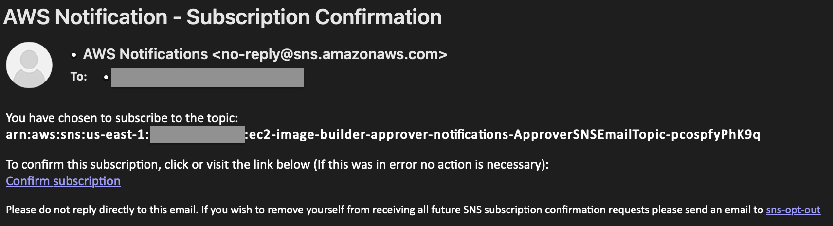
  1. After running the deployment, you will receive an email prompting you to confirm the Subscription at the approver email address. Choose Confirm subscription.

SNS Topic Subscription confirmation email

  1. This leads to the following screen, which shows that your subscription is confirmed.

subscription-confirmation

  1. Repeat the previous 2 steps for the target email address.

Step 3: Run the pipeline from the Image Builder console

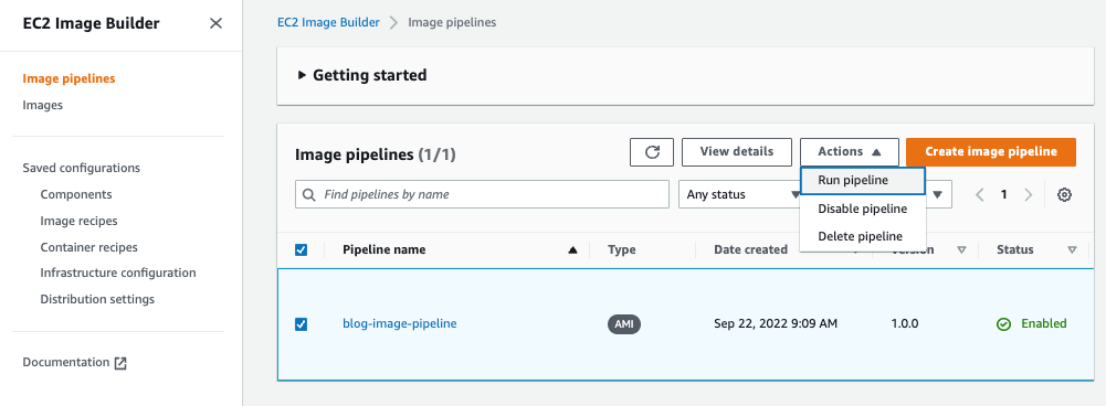
  1. In the Image Builder console, under Image pipelines, select the checkbox next to the Pipeline created, choose Actions, and select Run pipeline.

run-image-builder-pipeline

Note: The pipeline takes approximately 20 – 30 minutes to complete.

Step 4: [Optional] Launch an Amazon EC2 instance from the built AMI

If you have a requirement to manually validate the AMI before sharing it with other accounts or to the AWS organization an approver will launch an Amazon EC2 instance from the built AMI and conduct manual tests on the EC2 instance to make sure it is functional.

  1. In the Amazon EC2 console, under Images, choose AMIs. Validate that the AMI is created.

ami-in-account-a

  1. Follow AWS docs: Launching an EC2 instances from a custom AMI for steps on how to launch an Amazon EC2 instance from the AMI.

Step 5: Select the approval URL in the email sent

  1. When the pipeline is run successfully, you will receive another email with a URL to approve the AMI.

approval-email

  1. Before clicking on the Approve link, you must assume the IAM Role that is set as an approver for the Systems Manager step.
  2. In the CloudFormation console, choose the stack that was deployed.

cloudformation-stack

4. Choose Outputs and copy the IAM Role name.

ssm-approval-role-output

5. While logged in as the IAM Principal that has permissions to assume the approval IAM Role, follow the instructions at AWS IAM documentation for switching a role using the console to assume the approval role.
In the Switch Role page, in Role paste the name of the IAM Role that you copied in the previous step.

Note: This IAM Role was deployed with minimum permissions. Hence, seeing warning messages in the console is expected after assuming this role.

switch-role

6. Now in the approval email, select the Approve URL. This leads to the Systems Manager console. Choose Submit.

approve-console

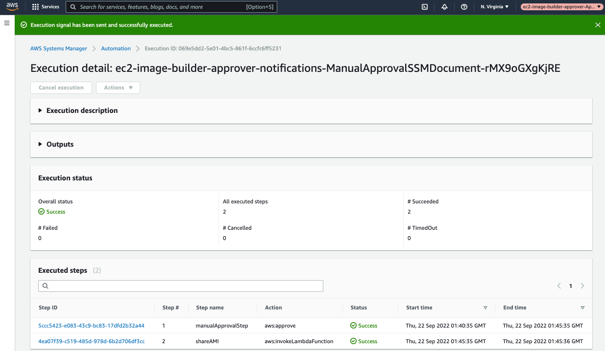
7. After approving the manual step, the second step is executed, which shares the AMI to the target account.

automation-step-success

Step 6: Verify that the AMI is shared to Account B

  1. Log in to Account B.
  2. In the Amazon EC2 console, under Images, choose AMIs. Then, in the dropdown, choose Private images. Validate that the AMI is shared.

verify-ami-in-account-b

  1. Verify that a success email notification was sent to the target account email address provided.

target-email

Clean up

This section provides the necessary information for deleting various resources created as part of this post.

  1. Deregister the AMIs that were created and shared.
    1. Log in to Account A and follow the steps at AWS documentation: Deregister your Linux AMI.
  2. Delete the CloudFormation stack. For instructions, refer to Deleting a stack on the AWS CloudFormation console.

Conclusion

In this post, we explained how to enable approval notifications for an Image Builder pipeline before AMIs are shared to other accounts. This solution can be extended to share to more than one AWS account or even to an AWS organization. With this solution, you will be notified when new golden images are created, allowing you to verify the accuracy of their configuration before sharing them to for wider use. This reduces the possibility of sharing AMIs with misconfigurations that the written tests may not have identified.

We invite you to experiment with different AMIs created using Image Builder, and with different Image Builder components. Check out this GitHub repository for various examples that use Image Builder. Also check out this blog on Image builder integrations with EC2 Auto Scaling Instance Refresh. Let us know your questions and findings in the comments, and have fun!

Fine-tuning Operations at Slice using AWS DevOps Guru

Post Syndicated from Adnan Bilwani original https://aws.amazon.com/blogs/devops/fine-tuning-operations-at-slice-using-aws-devops-guru/

This guest post was authored by Sapan Jain, DevOps Engineer at Slice, and edited by Sobhan Archakam and Adnan Bilwani, at AWS.

Slice empowers over 18,000 independent pizzerias with the modern tools that have grown the major restaurant chains. By uniting these small businesses with specialized technology, marketing, data insights, and shared services, Slice enables them to serve their digitally-minded customers and move away from third-party apps. Using Amazon DevOps Guru, Slice is able to fine-tune their operations to better support these customers.

Serial tech entrepreneur Ilir Sela started Slice to modernize and support his family’s New York City pizzerias. Today, the company partners with restaurants in 3,000 cities and all 50 states, forming the nation’s largest pizza network. For more information, visit slicelife.com.

Slice’s challenge

At Slice, we manage a wide variety of systems, services, and platforms, all with varying levels of complexity. Observability, monitoring, and log aggregation are things we excel at, and they’re always critical for our platform engineering team. However, deriving insights from this data still requires some manual investigation, particularly when dealing with operational anomalies and/or misconfigurations.

To gain automated insights into our services and resources, Slice conducted a proof-of-concept utilizing Amazon DevOps Guru to analyze a small selection of AWS resources. Amazon DevOps Guru identified potential issues in our environment, resulting in actionable insights (ultimately leading to remediation). As a result of this analysis, we enabled Amazon DevOps Guru account-wide, thereby leading to numerous insights into our production environment.

Insights with Amazon DevOps Guru

After we configured Amazon DevOps Guru to begin its account-wide analysis, we left the tool alone to begin the process of collecting and analyzing data. We immediately began seeing some actionable insights for various production AWS resources, some of which are highlighted in the following section:

Amazon DynamoDB Point-in-time recovery

Amazon DynamoDB offers a point-in-time recovery (PITR) feature that provides continuous backups of your DynamoDB data for 35 days to help you protect against accidental write or deletes. If enabled, this lets you restore your respective table to a previous state. Amazon DevOps Guru identified several tables in our environment that had PITR disabled, along with a corresponding Recommendation.

The graphic shows proactive insights for the last 1 month. The one insight shown is 'Dynamo Table Point in Time Recovery not enabled' with a status of OnGoing and a severity of low.

The graphic shows proactive insights for the last 1 month. The one insight shown is 'Dynamo Table Point in Time Recovery not enabled' with a status of OnGoing and a severity of low.

Figure 1. The graphic shows proactive insights for the last 1 month. The one insight shown is ‘Dynamo Table Point in Time Recovery not enabled’ with a status of OnGoing and a severity of low.

Elasticache anomalous evictions

Amazon Elasticache for Redis is used by a handful of our services to cache any relevant application data. Amazon DevOps Guru identified that one of our instances was exhibiting anomalous behavior regarding its cache eviction rate. Essentially, due to the memory pressure of the instance, the eviction rate of cache entries began to increase. DevOps Guru recommended revisiting the sizing of this instance and scaling it vertically or horizontally, where appropriate.

The graph shows the metric: count of ElastiCache evictions plotted for the time period Jul 3, 20:35 to Jul 3, 21:35 UTC. A highlighted section shows that the evictions increased to a peak of 2500 between 21:00 and 21:08. Outside of this interval the evictions are below 500.

The graph shows the metric: count of ElastiCache evictions plotted for the time period Jul 3, 20:35 to Jul 3, 21:35 UTC. A highlighted section shows that the evictions increased to a peak of 2500 between 21:00 and 21:08. Outside of this interval the evictions are below 500.

Figure 2. The graph shows the metric: count of ElastiCache evictions plotted for the time period Jul 3, 20:35 to Jul 3, 21:35 UTC. A highlighted section shows that the evictions increased to a peak of 2500 between 21:00 and 21:08. Outside of this interval the evictions are below 500

AWS Lambda anomalous errors

We manage a few AWS Lambda functions that all serve different purposes. During the beginning of normal work day, we began to see increased error rates for a particular function resulting in an exception being thrown. DevOps Guru was able to detect the increase in error rates and flag them as anomalous. Although retries in this case wouldn’t have solved the problem, it did increase our visibility into the issue (which was also corroborated by our APM platform).

The graph shows the metric: count of AWS/Lambda errors plotted between 11:00 and 13:30 on Jul 6. The sections between the times 11:23 and 12:15 and at 12:37 and 13:13 UTC are highlighted to show the anomalies.

Figure 3. The graph shows the metric: count of AWS/Lambda errors plotted between 11:00 and 13:30 on Jul 6. The sections between the times 11:23 and 12:15 and at 12:37 and 13:13 UTC are highlighted to show the anomalies

Figure 3. The graph shows the metric: count of AWS/Lambda errors plotted between 11:00 and 13:30 on Jul 6. The sections between the times 11:23 and 12:15 UTC are highlighted to show the anomalies

Conclusion

Amazon DevOps Guru integrated into our environment quickly, with no more additional configuration or setup aside from a few button clicks to enable the service. After reviewing several of the proactive insights that DevOps Guru provided, we could formulate plans of action regarding remediation. One specific case example of this is where DevOps Guru flagged several of our Lambda functions for not containing enough subnets. After triaging the finding, we discovered that we were lacking multi-AZ redundancy for several of those functions. As a result, we could implement a change that maximized our availability of those resources.

With the continuous analysis that DevOps Guru performs, we continue to gain new insights into the resources that we utilize and deploy in our environment. This lets us improve operationally while simultaneously maintaining production stability.

About the author:

Adnan Bilwani

Adnan Bilwani is a Sr. Specialist Builders Experience at AWS and part of the AI for DevOps portfolio of services providing fully managed ML-based solutions to enhance your DevOps workflows.

Sobhan Archakam

Sobhan Archakam is a Senior Technical Account Manager at Amazon Web Services. He provides advocacy and guidance to Enterprise Customers to plan, build, deploy and operate solutions at scale using best practices.

Sapan Jain

Sapan Jain is a DevOps Engineer at Slice. He provides support in all facets of DevOps, and has an interest in performance, observability, automation, and troubleshooting.

Best Practices for Hosting Regulated Gaming Workloads in AWS Local Zones and on AWS Outposts

Post Syndicated from Sheila Busser original https://aws.amazon.com/blogs/compute/best-practices-for-hosting-regulated-gaming-workloads-in-aws-local-zones-and-on-aws-outposts/

This blog post is written by Shiv Bhatt, Manthan Raval, and Pawan Matta, who are Senior Solutions Architects with AWS.

Many industries are subject to regulations that are created to protect the interests of the various stakeholders. For some industries, the specific details of the regulatory requirements influence not only the organization’s operations, but also their decisions for adopting new technology. In this post, we highlight the workload residency challenges that you may encounter when you deploy regulated gaming workloads, and how AWS Local Zones and AWS Outposts can help you address those challenges.

Regulated gaming workloads and residency requirements

A regulated gaming workload is a type of workload that’s subject to federal, state, local, or tribal laws related to the regulation of gambling and real money gaming. Examples of these workloads include sports betting, horse racing, casino, poker, lottery, bingo, and fantasy sports. The operators provide gamers with access to these workloads through online and land-based channels, and they’re required to follow various regulations required in their jurisdiction. Some regulations define specific workload residency requirements, and depending on the regulatory agency, the regulations could require that workloads be hosted within a specific city, state, province, or country. For example, in the United States, different state and tribal regulatory agencies dictate whether and where gaming operations are legal in a state, and who can operate. The agencies grant licenses to the operators of regulated gaming workloads, which then govern who can operate within the state, and sometimes, specifically where these workloads can be hosted. In addition, federal legislation can also constrain how regulated gaming workloads can be operated. For example, the United States Federal Wire Act makes it illegal to facilitate bets or wagers on sporting events across state lines. This regulation requires that operators make sure that users who place bets in a specific state are also within the borders of that state.

Benefits of using AWS edge infrastructure with regulated gaming workloads

The use of AWS edge infrastructure, specifically Local Zones and Outposts to host a regulated gaming workload, can help you meet workload residency requirements. You can manage Local Zones and Outposts by using the AWS Management Console or by using control plane API operations, which lets you seamlessly consume compute, storage, and other AWS services.

Local Zones

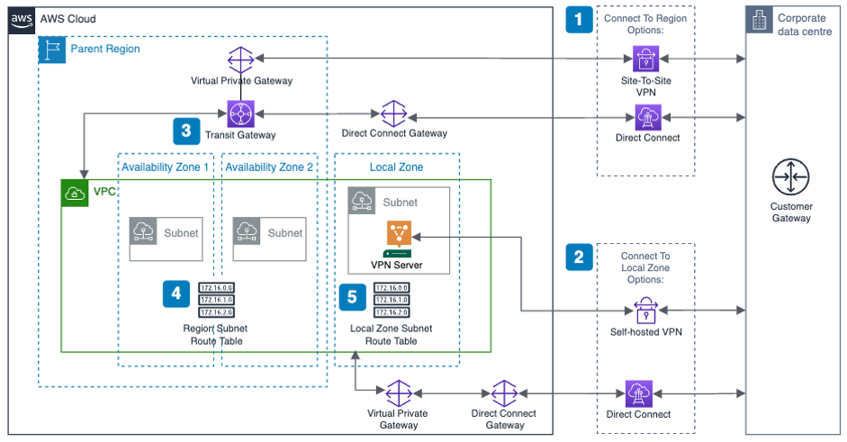
Local Zones are a type of AWS infrastructure deployment that place compute, storage, database, and other select services closer to large population, industry, and IT centers. Like AWS Regions, Local Zones enable you to innovate more quickly and bring new products to market sooner without having to worry about hardware and data center space procurement, capacity planning, and other forms of undifferentiated heavy-lifting. Local Zones have their own connections to the internet, and support AWS Direct Connect, so that workloads hosted in the Local Zone can serve local end-users with very low-latency communications. Local Zones are by default connected to a parent Region via Amazon’s redundant and high-bandwidth private network. This lets you extend Amazon Virtual Private Cloud (Amazon VPC) in the AWS Region to Local Zones. Furthermore, this provides applications hosted in AWS Local Zones with fast, secure, and seamless access to the broader portfolio of AWS services in the AWS Region. You can see the full list of AWS services supported in Local Zones on the AWS Local Zones features page.

You can start using Local Zones right away by enabling them in your AWS account. There are no setup fees, and as with the AWS Region, you pay only for the services that you use. There are three ways to pay for Amazon Elastic Compute Cloud (Amazon EC2) instances in Local Zones: On-Demand, Savings Plans, and Spot Instances. See the full list of cities where Local Zones are available on the Local Zones locations page.

Outposts

Outposts is a family of fully-managed solutions that deliver AWS infrastructure and services to most customer data center locations for a consistent hybrid experience. For a full list of countries and territories where Outposts is available, see the Outposts rack FAQs and Outposts servers FAQs. Outposts is available in various form factors, from 1U and 2U Outposts servers to 42U Outposts racks, and multiple rack deployments. To learn more about specific configuration options and pricing, see Outposts rack and Outposts servers.

You configure Outposts to work with a specific AWS Region using AWS Direct Connect or an internet connection, which lets you extend Amazon VPC in the AWS Region to Outposts. Like Local Zones, this provides applications hosted on Outposts with fast, secure, and seamless access to the broader portfolio of AWS services in the AWS Region. See the full list of AWS services supported on Outposts rack and on Outposts servers.

Choosing between AWS Regions, Local Zones, and Outposts

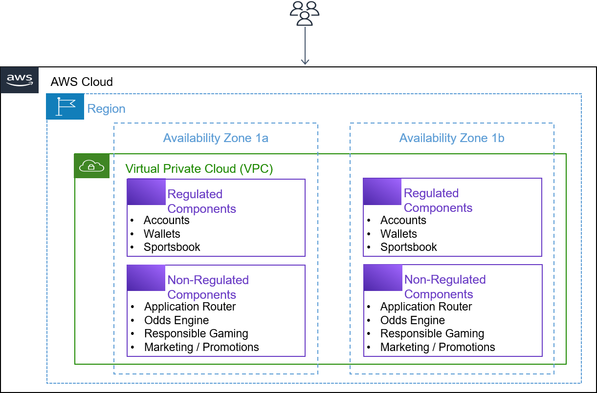
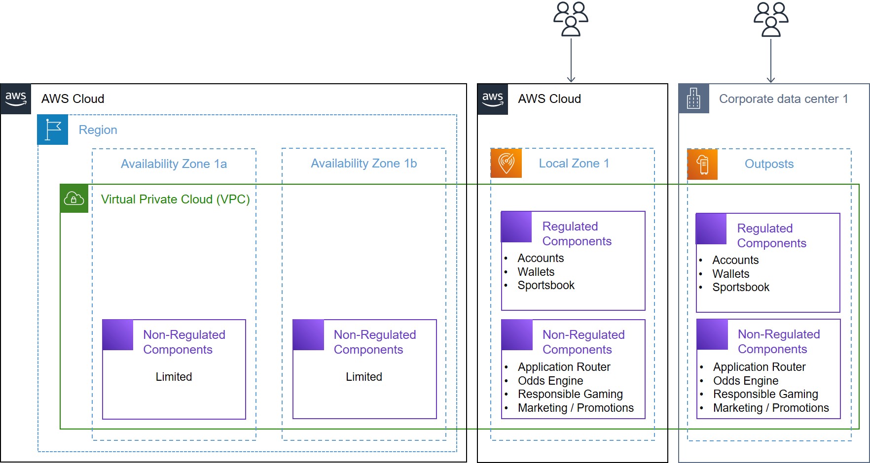
When you build and deploy a regulated gaming workload, you must assess the residency requirements carefully to make sure that your workload complies with regulations. As you make your assessment, we recommend that you consider separating your regulated gaming workload into regulated and non-regulated components. For example, for a sports betting workload, the regulated components might include sportsbook operation, and account and wallet management, while non-regulated components might include marketing, the odds engine, and responsible gaming. In describing the following scenarios, it’s assumed that regulated and non-regulated components must be fault-tolerant.

For hosting the non-regulated components of your regulated gaming workload, we recommend that you consider using an AWS Region instead of a Local Zone or Outpost. An AWS Region offers higher availability, larger scale, and a broader selection of AWS services.

For hosting regulated components, the type of AWS infrastructure that you choose will depend on which of the following scenarios applies to your situation:

  1. Scenario one: An AWS Region is available in your jurisdiction and local regulators have approved the use of cloud services for your regulated gaming workload.
  2. Scenario two: An AWS Region isn’t available in your jurisdiction, but a Local Zone is available, and local regulators have approved the use of cloud services for your regulated gaming workload.
  3. Scenario three: An AWS Region or Local Zone isn’t available in your jurisdiction, or local regulators haven’t approved the use of cloud services for your regulated gaming workload, but Outposts is available.

Let’s look at each of these scenarios in detail.

Scenario one: Use an AWS Region for regulated components

When local regulators have approved the use of cloud services for regulated gaming workloads, and an AWS Region is available in your jurisdiction, consider using an AWS Region rather than a Local Zone and Outpost. For example, in the United States, the State of Ohio has announced that it will permit regulated gaming workloads to be deployed in the cloud on infrastructure located within the state when sports betting goes live in January 2023. By using the US East (Ohio) Region, operators in the state don’t need to procure and manage physical infrastructure and data center space. Instead, they can use various compute, storage, database, analytics, and artificial intelligence/machine learning (AI/ML) services that are readily available in the AWS Region. You can host a regulated gaming workload entirely in a single AWS Region, which includes Availability Zones (AZs) – multiple, isolated locations within each AWS Region. By deploying your workload redundantly across at least two AZs, you can help make sure of the high availability, as shown in the following figure.

AWS Region hosting regulated and non-regulated components

Scenario two: Use a Local Zone for regulated components

A second scenario might be that local regulators have approved the use of cloud services for regulated gaming workloads, and an AWS Region isn’t available in your jurisdiction, but a Local Zone is available. In this scenario, consider using a Local Zone rather than Outposts. A Local Zone can support more elasticity in a more cost-effective way than Outposts can. However, you might also consider using a Local Zone and Outposts together to increase availability and scalability for regulated components. Let’s consider the State of Illinois, in the United States, which allows regulated gaming workloads to be deployed in the cloud, if workload residency requirements are met. Operators in this state can host regulated components in a Local Zone in Chicago, and they can also use Outposts in their data center in the same state, for high availability and disaster recovery, as shown in the following figure.

Route ingress gaming traffic through an AWS Region hosting non-regulated components, with a Local Zone and Outposts hosting regulated components

Scenario three: Use of Outposts for regulated components

When local regulators haven’t approved the use of cloud services for regulated gaming workloads, or when an AWS Region or Local Zone isn’t available in your jurisdiction, you can still choose to host your regulated gaming workloads on Outposts for a consistent cloud experience, if Outposts is available in your jurisdiction. If you choose to use Outposts, then note that as part of the shared responsibility model, customers are responsible for attesting to physical security and access controls around the Outpost, as well as environmental requirements for the facility, networking, and power. Use of Outposts requires you to procure and manage the data center within the city, state, province, or country boundary (as required by local regulations) that may be suitable to host regulated components, depending on the jurisdiction. Furthermore, you should procure and configure supported network connections between Outposts and the parent AWS Region. During the Outposts ordering process, you should account for the compute and network capacity required to support the peak load and availability design.

For a higher availability level, you should consider procuring and deploying two or more Outposts racks or Outposts servers in a data center. You might also consider deploying redundant network paths between Outposts and the parent AWS Region. However, depending on your business service level agreement (SLA) for regulated gaming workload, you might choose to spread Outposts racks across two or more isolated data centers within the same regulated boundary, as shown in the following figure.

Route ingress gaming traffic through an AWS Region hosting non-regulated components, with an Outposts hosting regulated components

Options to route ingress gaming traffic

You have two options to route ingress gaming traffic coming into your regulated and non-regulated components when you deploy the configurations that we described previously in Scenarios two and three. Your gaming traffic can come through to the AWS Region, or through the Local Zones or Outposts. Note that the benefits that we mentioned previously around selecting the AWS Region for deploying regulated and non-regulated components are the same when you select an ingress route.

Let’s discuss the benefits and trade offs for each of these options.

Option one: Route ingress gaming traffic through an AWS Region

If you choose to route ingress gaming traffic through an AWS Region, your regulated gaming workloads benefit from access to the wide range of tools, services, and capacity available in the AWS Region. For example, native AWS security services, like AWS WAF and AWS Shield, which provide protection against DDoS attacks, are currently only available in AWS Regions. Only traffic that you route into your workload through an AWS Region benefits from these services.

If you route gaming traffic through an AWS Region, and non-regulated components are hosted in an AWS Region, then traffic has a direct path to non-regulated components. In addition, gaming traffic destined to regulated components, hosted in a Local Zone and on Outposts, can be routed through your non-regulated components and a few native AWS services in the AWS Region, as shown in Figure 2.

Option two: Route ingress gaming traffic through a Local Zone or Outposts

Choosing to route ingress gaming traffic through a Local Zone or Outposts requires careful planning to make sure that tools, services, and capacity are available in that jurisdiction, as shown in the following figure. In addition, consider how choosing this route will influence the pillars of the AWS Well-Architected Framework. This route might require deploying and managing most of your non-regulated components in a Local Zone or on Outposts as well, including native AWS services that aren’t available in Local Zones or on Outposts. If you plan to implement this topology, then we recommend that you consider using AWS Partner solutions to replace the native AWS services that aren’t available in Local Zones or Outposts.

Route ingress gaming traffic through a Local Zone and Outposts that are hosting regulated and non-regulated components, with an AWS Region hosting limited non-regulated components

Conclusion

If you’re building regulated gaming workloads, then you might have to follow strict workload residency and availability requirements. In this post, we’ve highlighted how Local Zones and Outposts can help you meet these workload residency requirements by bringing AWS services closer to where they’re needed. We also discussed the benefits of using AWS Regions in compliment to the AWS edge infrastructure, and several reliability and cost design considerations.

Although this post provides information to consider when making choices about using AWS for regulated gaming workloads, you’re ultimately responsible for maintaining compliance with the gaming regulations and laws in your jurisdiction. You’re in the best position to determine and maintain ultimate responsibility for determining whether activities are legal, including evaluating the jurisdiction of the activities, how activities are made available, and whether specific technologies or services are required to make sure of compliance with the applicable law. You should always review these regulations and laws before you deploy regulated gaming workloads on AWS.

Common streaming data enrichment patterns in Amazon Kinesis Data Analytics for Apache Flink

Post Syndicated from Ali Alemi original https://aws.amazon.com/blogs/big-data/common-streaming-data-enrichment-patterns-in-amazon-kinesis-data-analytics-for-apache-flink/

Stream data processing allows you to act on data in real time. Real-time data analytics can help you have on-time and optimized responses while improving overall customer experience.

Apache Flink is a distributed computation framework that allows for stateful real-time data processing. It provides a single set of APIs for building batch and streaming jobs, making it easy for developers to work with bounded and unbounded data. Apache Flink provides different levels of abstraction to cover a variety of event processing use cases.

Amazon Kinesis Data Analytics is an AWS service that provides a serverless infrastructure for running Apache Flink applications. This makes it easy for developers to build highly available, fault tolerant, and scalable Apache Flink applications without needing to become an expert in building, configuring, and maintaining Apache Flink clusters on AWS.

Data streaming workloads often require data in the stream to be enriched via external sources (such as databases or other data streams). For example, assume you are receiving coordinates data from a GPS device and need to understand how these coordinates map with physical geographic locations; you need to enrich it with geolocation data. You can use several approaches to enrich your real-time data in Kinesis Data Analytics depending on your use case and Apache Flink abstraction level. Each method has different effects on the throughput, network traffic, and CPU (or memory) utilization. In this post, we cover these approaches and discuss their benefits and drawbacks.

Data enrichment patterns

Data enrichment is a process that appends additional context and enhances the collected data. The additional data often is collected from a variety of sources. The format and the frequency of the data updates could range from once in a month to many times in a second. The following table shows a few examples of different sources, formats, and update frequency.

Data Format Update Frequency
IP address ranges by country CSV Once a month
Company organization chart JSON Twice a year
Machine names by ID CSV Once a day
Employee information Table (Relational database) A few times a day
Customer information Table (Non-relational database) A few times an hour
Customer orders Table (Relational database) Many times a second

Based on the use case, your data enrichment application may have different requirements in terms of latency, throughput, or other factors. The remainder of the post dives deeper into different patterns of data enrichment in Kinesis Data Analytics, which are listed in the following table with their key characteristics. You can choose the best pattern based on the trade-off of these characteristics.

Enrichment Pattern Latency Throughput Accuracy if Reference Data Changes Memory Utilization Complexity
Pre-load reference data in Apache Flink Task Manager memory Low High Low High Low
Partitioned pre-loading of reference data in Apache Flink state Low High Low Low Low
Periodic Partitioned pre-loading of reference data in Apache Flink state Low High Medium Low Medium
Per-record asynchronous lookup with unordered map Medium Medium High Low Low
Per-record asynchronous lookup from an external cache system Low or Medium (Depending on Cache storage and implementation) Medium High Low Medium
Enriching streams using the Table API Low High High Low – Medium (depending on the selected join operator) Low

Enrich streaming data by pre-loading the reference data

When the reference data is small in size and static in nature (for example, country data including country code and country name), it’s recommended to enrich your streaming data by pre-loading the reference data, which you can do in several ways.

To see the code implementation for pre-loading reference data in various ways, refer to the GitHub repo. Follow the instructions in the GitHub repository to run the code and understand the data model.

Pre-loading of reference data in Apache Flink Task Manager memory

The simplest and also fastest enrichment method is to load the enrichment data into each of the Apache Flink task managers’ on-heap memory. To implement this method, you create a new class by extending the RichFlatMapFunction abstract class. You define a global static variable in your class definition. The variable could be of any type, the only limitation is that it should extend java.io.Serializable—for example, java.util.HashMap. Within the open() method, you define a logic that loads the static data into your defined variable. The open() method is always called first, during the initialization of each task in Apache Flink’s task managers, which makes sure the whole reference data is loaded before the processing begins. You implement your processing logic by overriding the processElement() method. You implement your processing logic and access the reference data by its key from the defined global variable.

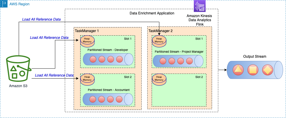
The following architecture diagram shows the full reference data load in each task slot of the task manager.

diagram shows the full reference data load in each task slot of the task manager.

This method has the following benefits:

  • Easy to implement
  • Low latency
  • Can support high throughput

However, it has the following disadvantages:

  • If the reference data is large in size, the Apache Flink task manager may run out of memory.
  • Reference data can become stale over a period of time.
  • Multiple copies of the same reference data are loaded in each task slot of the task manager.
  • Reference data should be small to fit in the memory allocated to a single task slot. In Kinesis Data Analytics, each Kinesis Processing Unit (KPU) has 4 GB of memory, out of which 3 GB can be used for heap memory. If ParallelismPerKPU in Kinesis Data Analytics is set to 1, one task slot runs in each task manager, and the task slot can use the whole 3 GB of heap memory. If ParallelismPerKPU is set to a value greater than 1, the 3 GB of heap memory is distributed across multiple task slots in the task manager. If you’re deploying Apache Flink in Amazon EMR or in a self-managed mode, you can tune taskmanager.memory.task.heap.size to increase the heap memory of a task manager.

Partitioned pre-loading of reference data in Apache Flink State

In this approach, the reference data is loaded and kept in the Apache Flink state store at the start of the Apache Flink application. To optimize the memory utilization, first the main data stream is divided by a specified field via the keyBy() operator across all task slots. Furthermore, only the portion of the reference data that corresponds to each task slot is loaded in the state store.

This is achieved in Apache Flink by creating the class PartitionPreLoadEnrichmentData, extending the RichFlatMapFunction abstract class. Within the open method, you override the ValueStateDescriptor method to create a state handle. In the referenced example, the descriptor is named locationRefData, the state key type is String, and the value type is Location. In this code, we use ValueState compared to MapState because we only hold the location reference data for a particular key. For example, when we query Amazon S3 to get the location reference data, we query for the specific role and get a particular location as a value.

In Apache Flink, ValueState is used to hold a specific value for a key, whereas MapState is used to hold a combination of key-value pairs.

This technique is useful when you have a large static dataset that is difficult to fit in memory as a whole for each partition.

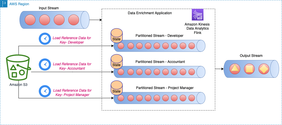
The following architecture diagram shows the load of reference data for the specific key for each partition of the stream.

diagram shows the load of reference data for the specific key for each partition of the stream.

For example, our reference data in the sample GitHub code has roles which are mapped to each building. Because the stream is partitioned by roles, only the specific building information per role is required to be loaded for each partition as the reference data.

This method has the following benefits:

  • Low latency.
  • Can support high throughput.
  • Reference data for specific partition is loaded in the keyed state.
  • In Kinesis Data Analytics, the default state store configured is RocksDB. RocksDB can utilize a significant portion of 1 GB of managed memory and 50 GB of disk space provided by each KPU. This provides enough room for the reference data to grow.

However, it has the following disadvantages:

  • Reference data can become stale over a period of time

Periodic partitioned pre-loading of reference data in Apache Flink State

This approach is a fine-tune of the previous technique, where each partitioned reference data is reloaded on a periodic basis to refresh the reference data. This is useful if your reference data changes occasionally.

The following architecture diagram shows the periodic load of reference data for the specific key for each partition of the stream.

diagram shows the periodic load of reference data for the specific key for each partition of the stream.

In this approach, the class PeriodicPerPartitionLoadEnrichmentData is created, extending the KeyedProcessFunction class. Similar to the previous pattern, in the context of the GitHub example, ValueState is recommended here because each partition only loads a single value for the key. In the same way as mentioned earlier, in the open method, you define the ValueStateDescriptor to handle the value state and define a runtime context to access the state.

Within the processElement method, load the value state and attach the reference data (in the referenced GitHub example, buildingNo to the customer data). Also register a timer service to be invoked when the processing time passes the given time. In the sample code, the timer service is scheduled to be invoked periodically (for example, every 60 seconds). In the onTimer method, update the state by making a call to reload the reference data for the specific role.

This method has the following benefits:

  • Low latency.
  • Can support high throughput.
  • Reference data for specific partitions is loaded in the keyed state.
  • Reference data is refreshed periodically.
  • In Kinesis Data Analytics, the default state store configured is RocksDB. Also, 50 GB of disk space provided by each KPU. This provides enough room for the reference data to grow.

However, it has the following disadvantages:

  • If the reference data changes frequently, the application still has stale data depending on how frequently the state is reloaded
  • The application can face load spikes during reload of reference data

Enrich streaming data using per-record lookup

Although pre-loading of reference data provides low latency and high throughput, it may not be suitable for certain types of workloads, such as the following:

  • Reference data updates with high frequency
  • Apache Flink needs to make an external call to compute the business logic
  • Accuracy of the output is important and the application shouldn’t use stale data

Normally, for these types of use cases, developers trade-off high throughput and low latency for data accuracy. In this section, you learn about a few of common implementations for per-record data enrichment and their benefits and disadvantages.

Per-record asynchronous lookup with unordered map

In a synchronous per-record lookup implementation, the Apache Flink application has to wait until it receives the response after sending every request. This causes the processor to stay idle for a significant period of processing time. Instead, the application can send a request for other elements in the stream while it waits for the response for the first element. This way, the wait time is amortized across multiple requests and therefore it increases the process throughput. Apache Flink provides asynchronous I/O for external data access. While using this pattern, you have to decide between unorderedWait (where it emits the result to the next operator as soon as the response is received, disregarding the order of the element on the stream) and orderedWait (where it waits until all inflight I/O operations complete, then sends the results to the next operator in the same order as original elements were placed on the stream). Usually, when downstream consumers disregard the order of the elements in the stream, unorderedWait provides better throughput and less idle time. Visit Enrich your data stream asynchronously using Kinesis Data Analytics for Apache Flink to learn more about this pattern.

The following architecture diagram shows how an Apache Flink application on Kinesis Data Analytics does asynchronous calls to an external database engine (for example Amazon DynamoDB) for every event in the main stream.

diagram shows how an Apache Flink application on Kinesis Data Analytics does asynchronous calls to an external database engine (for example Amazon DynamoDB) for every event in the main stream.

This method has the following benefits:

  • Still reasonably simple and easy to implement
  • Reads the most up-to-date reference data

However, it has the following disadvantages:

  • It generates a heavy read load for the external system (for example, a database engine or an external API) that hosts the reference data
  • Overall, it might not be suitable for systems that require high throughput with low latency

Per-record asynchronous lookup from an external cache system

A way to enhance the previous pattern is to use a cache system to enhance the read time for every lookup I/O call. You can use Amazon ElastiCache for caching, which accelerates application and database performance, or as a primary data store for use cases that don’t require durability like session stores, gaming leaderboards, streaming, and analytics. ElastiCache is compatible with Redis and Memcached.

For this pattern to work, you must implement a caching pattern for populating data in the cache storage. You can choose between a proactive or reactive approach depending your application objectives and latency requirements. For more information, refer to Caching patterns.

The following architecture diagram shows how an Apache Flink application calls to read the reference data from an external cache storage (for example, Amazon ElastiCache for Redis). Data changes must be replicated from the main database (for example, Amazon Aurora) to the cache storage by implementing one of the caching patterns.

diagram shows how an Apache Flink application calls to read the reference data from an external cache storage (for example, Amazon ElastiCache for Redis). Data changes must be replicated from the main database (for example, Amazon Aurora) to the cache storage by implementing one of the caching patterns.

Implementation for this data enrichment pattern is similar to the per-record asynchronous lookup pattern; the only difference is that the Apache Flink application makes a connection to the cache storage, instead of connecting to the primary database.

This method has the following benefits:

  • Better throughput because caching can accelerate application and database performance
  • Protects the primary data source from the read traffic created by the stream processing application
  • Can provide lower read latency for every lookup call
  • Overall, might not be suitable for medium to high throughput systems that want to improve data freshness

However, it has the following disadvantages:

  • Additional complexity of implementing a cache pattern for populating and syncing the data between the primary database and the cache storage
  • There is a chance for the Apache Flink stream processing application to read stale reference data depending on what caching pattern is implemented
  • Depending on the chosen cache pattern (proactive or reactive), the response time for each enrichment I/O may differ, therefore the overall processing time of the stream could be unpredictable

Alternatively, you can avoid these complexities by using the Apache Flink JDBC connector for Flink SQL APIs. We discuss enrichment stream data via Flink SQL APIs in more detail later in this post.

Enrich stream data via another stream

In this pattern, the data in the main stream is enriched with the reference data in another data stream. This pattern is good for use cases in which the reference data is updated frequently and it’s possible to perform change data capture (CDC) and publish the events to a data streaming service such as Apache Kafka or Amazon Kinesis Data Streams. This pattern is useful in the following use cases, for example:

  • Customer purchase orders are published to a Kinesis data stream, and then join with customer billing information in a DynamoDB stream
  • Data events captured from IoT devices should enrich with reference data in a table in Amazon Relational Database Service (Amazon RDS)
  • Network log events should enrich with the machine name on the source (and the destination) IP addresses

The following architecture diagram shows how an Apache Flink application on Kinesis Data Analytics joins data in the main stream with the CDC data in a DynamoDB stream.

diagram shows how an Apache Flink application on Kinesis Data Analytics joins data in the main stream with the CDC data in a DynamoDB stream.

To enrich streaming data from another stream, we use a common stream to stream join patterns, which we explain in the following sections.

Enrich streams using the Table API

Apache Flink Table APIs provide higher abstraction for working with data events. With Table APIs, you can define your data stream as a table and attach the data schema to it.

In this pattern, you define tables for each data stream and then join those tables to achieve the data enrichment goals. Apache Flink Table APIs support different types of join conditions, like inner join and outer join. However, you want to avoid those if you’re dealing with unbounded streams because those are resource intensive. To limit the resource utilization and run joins effectively, you should use either interval or temporal joins. An interval join requires one equi-join predicate and a join condition that bounds the time on both sides. To better understand how to implement an interval join, refer to Get started with Apache Flink SQL APIs in Kinesis Data Analytics Studio.

Compared to interval joins, temporal table joins don’t work with a time period within which different versions of a record are kept. Records from the main stream are always joined with the corresponding version of the reference data at the time specified by the watermark. Therefore, fewer versions of the reference data remain in the state.

Note that the reference data may or may not have a time element associated with it. If it doesn’t, you may need to add a processing time element for the join with the time-based stream.

In the following example code snippet, the update_time column is added to the currency_rates reference table from the change data capture metadata such as Debezium. Furthermore, it’s used to define a watermark strategy for the table.

CREATE TABLE currency_rates (
    currency STRING,
    conversion_rate DECIMAL(32, 2),
    update_time TIMESTAMP(3) METADATA FROM `values.source.timestamp` VIRTUAL,
        WATERMARK FOR update_time AS update_time,
    PRIMARY KEY(currency) NOT ENFORCED
) WITH (
   'connector' = 'kafka',
   'value.format' = 'debezium-json',
   /* ... */
);

This method has the following benefits:
  • Easy to implement
  • Low latency
  • Can support high throughput when reference data is a data stream

SQL APIs provide higher abstractions over how the data is processed. For more complex logic around how the join operator should process, we recommend you always start with SQL APIs first and use DataStream APIs if you really need to.

Conclusion

In this post, we demonstrated different data enrichment patterns in Kinesis Data Analytics. You can use these patterns and find the one that addresses your needs and quickly develop a stream processing application.

For further reading on Kinesis Data Analytics, visit the official product page.


About the Authors

About the author Ali AlemiAli Alemi is a Streaming Specialist Solutions Architect at AWS. Ali advises AWS customers with architectural best practices and helps them design real-time analytics data systems that are reliable, secure, efficient, and cost-effective. He works backward from customers’ use cases and designs data solutions to solve their business problems. Prior to joining AWS, Ali supported several public sector customers and AWS consulting partners in their application modernization journey and migration to the cloud.

About the author Subham RakshitSubham Rakshit is a Streaming Specialist Solutions Architect for Analytics at AWS based in the UK. He works with customers to design and build search and streaming data platforms that help them achieve their business objective. Outside of work, he enjoys spending time solving jigsaw puzzles with his daughter.

About the author Dr. Sam MokhtariDr. Sam Mokhtari is a Senior Solutions Architect in AWS. His main area of depth is data and analytics, and he has published more than 30 influential articles in this field. He is also a respected data and analytics advisor who led several large-scale implementation projects across different industries, including energy, health, telecom, and transport.

Design considerations for Amazon EMR on EKS in a multi-tenant Amazon EKS environment

Post Syndicated from Lotfi Mouhib original https://aws.amazon.com/blogs/big-data/design-considerations-for-amazon-emr-on-eks-in-a-multi-tenant-amazon-eks-environment/

Many AWS customers use Amazon Elastic Kubernetes Service (Amazon EKS) in order to take advantage of Kubernetes without the burden of managing the Kubernetes control plane. With Kubernetes, you can centrally manage your workloads and offer administrators a multi-tenant environment where they can create, update, scale, and secure workloads using a single API. Kubernetes also allows you to improve resource utilization, reduce cost, and simplify infrastructure management to support different application deployments. This model is beneficial for those running Apache Spark workloads, for several reasons. For example, it allows you to have multiple Spark environments running concurrently with different configurations and dependencies that are segregated from each other through Kubernetes multi-tenancy features. In addition, the same cluster can be used for various workloads like machine learning (ML), host applications, data streaming and thereby reducing operational overhead of managing multiple clusters.

AWS offers Amazon EMR on EKS, a managed service that enables you to run your Apache Spark workloads on Amazon EKS. This service uses the Amazon EMR runtime for Apache Spark, which increases the performance of your Spark jobs so that they run faster and cost less. When you run Spark jobs on EMR on EKS and not on self-managed Apache Spark on Kubernetes, you can take advantage of automated provisioning, scaling, faster runtimes, and the development and debugging tools that Amazon EMR provides

In this post, we show how to configure and run EMR on EKS in a multi-tenant EKS cluster that can used by your various teams. We tackle multi-tenancy through four topics: network, resource management, cost management, and security.

Concepts

Throughout this post, we use terminology that is either specific to EMR on EKS, Spark, or Kubernetes:

  • Multi-tenancy – Multi-tenancy in Kubernetes can come in three forms: hard multi-tenancy, soft multi-tenancy and sole multi-tenancy. Hard multi-tenancy means each business unit or group of applications gets a dedicated Kubernetes; there is no sharing of the control plane. This model is out of scope for this post. Soft multi-tenancy is where pods might share the same underlying compute resource (node) and are logically separated using Kubernetes constructs through namespaces, resource quotas, or network policies. A second way to achieve multi-tenancy in Kubernetes is to assign pods to specific nodes that are pre-provisioned and allocated to a specific team. In this case, we talk about sole multi-tenancy. Unless your security posture requires you to use hard or sole multi-tenancy, you would want to consider using soft multi-tenancy for the following reasons:
    • Soft multi-tenancy avoids underutilization of resources and waste of compute resources.
    • There is a limited number of managed node groups that can be used by Amazon EKS, so for large deployments, this limit can quickly become a limiting factor.
    • In sole multi-tenancy there is high chance of ghost nodes with no pods scheduled on them due to misconfiguration as we force pods into dedicated nodes with label, taints and tolerance and anti-affinity rules.
  • Namespace – Namespaces are core in Kubernetes and a pillar to implement soft multi-tenancy. With namespaces, you can divide the cluster into logical partitions. These partitions are then referenced in quotas, network policies, service accounts, and other constructs that help isolate environments in Kubernetes.
  • Virtual cluster – An EMR virtual cluster is mapped to a Kubernetes namespace that Amazon EMR is registered with. Amazon EMR uses virtual clusters to run jobs and host endpoints. Multiple virtual clusters can be backed by the same physical cluster. However, each virtual cluster maps to one namespace on an EKS cluster. Virtual clusters don’t create any active resources that contribute to your bill or require lifecycle management outside the service.
  • Pod template – In EMR on EKS, you can provide a pod template to control pod placement, or define a sidecar container. This pod template can be defined for executor pods and driver pods, and stored in an Amazon Simple Storage Service (Amazon S3) bucket. The S3 locations are then submitted as part of the applicationConfiguration object that is part of configurationOverrides, as defined in the EMR on EKS job submission API.

Security considerations

In this section, we address security from different angles. We first discuss how to protect IAM role that is used for running the job. Then address how to protect secrets use in jobs and finally we discuss how you can protect data while it is processed by Spark.

IAM role protection

A job submitted to EMR on EKS needs an AWS Identity and Access Management (IAM) execution role to interact with AWS resources, for example with Amazon S3 to get data, with Amazon CloudWatch Logs to publish logs, or use an encryption key in AWS Key Management Service (AWS KMS). It’s a best practice in AWS to apply least privilege for IAM roles. In Amazon EKS, this is achieved through IRSA (IAM Role for Service Accounts). This mechanism allows a pod to assume an IAM role at the pod level and not at the node level, while using short-term credentials that are provided through the EKS OIDC.

IRSA creates a trust relationship between the EKS OIDC provider and the IAM role. This method allows only pods with a service account (annotated with an IAM role ARN) to assume a role that has a trust policy with the EKS OIDC provider. However, this isn’t enough, because it would allow any pod with a service account within the EKS cluster that is annotated with a role ARN to assume the execution role. This must be further scoped down using conditions on the role trust policy. This condition allows the assume role to happen only if the calling service account is the one used for running a job associated with the virtual cluster. The following code shows the structure of the condition to add to the trust policy:

{
    "Version": "2012-10-17",
    "Statement": [
        {
            "Effect": "Allow",
            "Principal": {
                "Federated": <OIDC provider ARN >
            },
            "Action": "sts:AssumeRoleWithWebIdentity"
            "Condition": { "StringLike": { “<OIDC_PROVIDER>:sub": "system:serviceaccount:<NAMESPACE>:emr-containers-sa-*-*-<AWS_ACCOUNT_ID>-<BASE36_ENCODED_ROLE_NAME>”} }
        }
    ]
}

To scope down the trust policy using the service account condition, you need to run the following the command with AWS CLI:

aws emr-containers update-role-trust-policy \
–cluster-name cluster \
–namespace namespace \
–role-name iam_role_name_for_job_execution

The command will the add the service account that will be used by the spark client, Jupyter Enterprise Gateway, Spark kernel, driver or executor. The service accounts name have the following structure emr-containers-sa-*-*-<AWS_ACCOUNT_ID>-<BASE36_ENCODED_ROLE_NAME>.

In addition to the role segregation offered by IRSA, we recommend blocking access to instance metadata because a pod can still inherit the rights of the instance profile assigned to the worker node. For more information about how you can block access to metadata, refer to Restrict access to the instance profile assigned to the worker node.

Secret protection

Sometime a Spark job needs to consume data stored in a database or from APIs. Most of the time, these are protected with a password or access key. The most common way to pass these secrets is through environment variables. However, in a multi-tenant environment, this means any user with access to the Kubernetes API can potentially access the secrets in the environment variables if this access isn’t scoped well to the namespaces the user has access to.

To overcome this challenge, we recommend using a Secrets store like AWS Secrets Manager that can be mounted through the Secret Store CSI Driver. The benefit of using Secrets Manager is the ability to use IRSA and allow only the role assumed by the pod access to the given secret, thereby improving your security posture. You can refer to the best practices guide for sample code showing the use of Secrets Manager with EMR on EKS.

Spark data encryption

When a Spark application is running, the driver and executors produce intermediate data. This data is written to the node local storage. Anyone who is able to exec into the pods would be able to read this data. Spark supports encryption of this data, and it can be enabled by passing --conf spark.io.encryption.enabled=true. Because this configuration adds performance penalty, we recommend enabling data encryption only for workloads that store and access highly sensitive data and in untrusted environments.

Network considerations

In this section we discuss how to manage networking within the cluster as well as outside the cluster. We first address how Spark handle cross executors and driver communication and how to secure it. Then we discuss how to restrict network traffic between pods in the EKS cluster and allow only traffic destined to EMR on EKS. Last, we discuss how to restrict traffic of executors and driver pods to external AWS service traffic using security groups.

Network encryption

The communication between the driver and executor uses RPC protocol and is not encrypted. Starting with Spark 3 in the Kubernetes backed cluster, Spark offers a mechanism to encrypt communication using AES encryption.

The driver generates a key and shares it with executors through the environment variable. Because the key is shared through the environment variable, potentially any user with access to the Kubernetes API (kubectl) can read the key. We recommend securing access so that only authorized users can have access to the EMR virtual cluster. In addition, you should set up Kubernetes role-based access control in such a way that the pod spec in the namespace where the EMR virtual cluster runs is granted to only a few selected service accounts. This method of passing secrets through the environment variable would change in the future with a proposal to use Kubernetes secrets.

To enable encryption, RPC authentication must also be enabled in your Spark configuration. To enable encryption in-transit in Spark, you should use the following parameters in your Spark config:

--conf spark.authenticate=true

--conf spark.network.crypto.enabled=true

Note that these are the minimal parameters to set; refer to Encryption from the complete list of parameters.

Additionally, applying encryption in Spark has a negative impact on processing speed. You should only apply it when there is a compliance or regulation need.

Securing Network traffic within the cluster

In Kubernetes, by default pods can communicate over the network across different namespaces in the same cluster. This behavior is not always desirable in a multi-tenant environment. In some instances, for example in regulated industries, to be compliant you want to enforce strict control over the network and send and receive traffic only from the namespace that you’re interacting with. For EMR on EKS, it would be the namespace associated to the EMR virtual cluster. Kubernetes offers constructs that allow you to implement network policies and define fine-grained control over the pod-to-pod communication. These policies are implemented by the CNI plugin; in Amazon EKS, the default plugin would be the VPC CNI. A policy is defined as follows and is applied with kubectl:

Kind: NetworkPolicy
metadata:
  name: default-np-ns1
  namespace: <EMR-VC-NAMESPACE>
spec:
  podSelector: {}
  policyTypes:
  - Ingress
  - Egress
  ingress:
  - from:
    - namespaceSelector:
        matchLabels:
          nsname: <EMR-VC-NAMESPACE>

Network traffic outside the cluster

In Amazon EKS, when you deploy pods on Amazon Elastic Compute Cloud (Amazon EC2) instances, all the pods use the security group associated with the node. This can be an issue if your pods (executor pods) are accessing a data source (namely a database) that allows traffic based on the source security group. Database servers often restrict network access only from where they are expecting it. In the case of a multi-tenant EKS cluster, this means pods from other teams that shouldn’t have access to the database servers, would be able to send traffic to it.

To overcome this challenge, you can use security groups for pods. This feature allows you to assign a specific security group to your pods, thereby controlling the network traffic to your database server or data source. You can also refer to the best practices guide for a reference implementation.

Cost management and chargeback

In a multi-tenant environment, cost management is a critical subject. You have multiple users from various business units, and you need to be able to precisely chargeback the cost of the compute resource they have used. At the beginning of the post, we introduced three models of multi-tenancy in Amazon EKS: hard multi-tenancy, soft multi-tenancy, and sole multi-tenancy. Hard multi-tenancy is out of scope because the cost tracking is trivial; all the resources are dedicated to the team using the cluster, which is not the case for sole multi-tenancy and soft multi-tenancy. In the next sections, we discuss these two methods to track the cost for each of model.

Soft multi-tenancy

In a soft multi-tenant environment, you can perform chargeback to your data engineering teams based on the resources they consumed and not the nodes allocated. In this method, you use the namespaces associated with the EMR virtual cluster to track how much resources were used for processing jobs. The following diagram illustrates an example.

Diagram to illustrate soft multi-tenancy

Diagram -1 Soft multi-tenancy

Tracking resources based on the namespace isn’t an easy task because jobs are transient in nature and fluctuate in their duration. However, there are partner tools available that allow you to keep track of the resources used, such as Kubecost, CloudZero, Vantage, and many others. For instructions on using Kubecost on Amazon EKS, refer to this blog post on cost monitoring for EKS customers.

Sole multi-tenancy

For sole multi-tenancy, the chargeback is done at the instance (node) level. Each member on your team uses a specific set of nodes that are dedicated to it. These nodes aren’t always running, and are spun up using the Kubernetes auto scaling mechanism. The following diagram illustrates an example.

Diagram to illustrate Sole tenancy

Diagram -2 Sole tenancy

With sole multi-tenancy, you use a cost allocation tag, which is an AWS mechanism that allows you to track how much each resource has consumed. Although the method of sole multi-tenancy isn’t efficient in terms of resource utilization, it provides a simplified strategy for chargebacks. With the cost allocation tag, you can chargeback a team based on all the resources they used, like Amazon S3, Amazon DynamoDB, and other AWS resources. The chargeback mechanism based on the cost allocation tag can be augmented using the recently launched AWS Billing Conductor, which allows you to issue bills internally for your team.

Resource management

In this section, we discuss considerations regarding resource management in multi-tenant clusters. We briefly discuss topics like sharing resources graciously, setting guard rails on resource consumption, techniques for ensuring resources for time sensitive and/or critical jobs, meeting quick resource scaling requirements and finally cost optimization practices with node selectors.

Sharing resources

In a multi-tenant environment, the goal is to share resources like compute and memory for better resource utilization. However, this requires careful capacity management and resource allocation to make sure each tenant gets their fair share. In Kubernetes, resource allocation is controlled and enforced by using ResourceQuota and LimitRange. ResourceQuota limits resources on the namespace level, and LimitRange allows you to make sure that all the containers are submitted with a resource requirement and a limit. In this section, we demonstrate how a data engineer or Kubernetes administrator can set up ResourceQuota as a LimitRange configuration.

The administrator creates one ResourceQuota per namespace that provides constraints for aggregate resource consumption:

apiVersion: v1
kind: ResourceQuota
metadata:
  name: compute-resources
  namespace: teamA
spec:
  hard:
    requests.cpu: "1000"
    requests.memory: 4000Gi
    limits.cpu: "2000"
    limits.memory: 6000Gi

For LimitRange, the administrator can review the following sample configuration. We recommend using default and defaultRequest to enforce the limit and request field on containers. Lastly, from a data engineer perspective while submitting the EMR on EKS jobs, you need to make sure the Spark parameters of resource requirements are within the range of the defined LimitRange. For example, in the following configuration, the request for spark.executor.cores=7 will fail because the max limit for CPU is 6 per container:

apiVersion: v1
kind: LimitRange
metadata:
  name: cpu-min-max
  namespace: teamA
spec:
  limits:
  - max:
      cpu: "6"
    min:
      cpu: "100m"
    default:
      cpu: "500m"
    defaultRequest:
      cpu: "100m"
    type: Container

Priority-based resource allocation

Diagram Illustrates an example of resource allocation with priority

Diagram – 3 Illustrates an example of resource allocation with priority.

As all the EMR virtual clusters share the same EKS computing platform with limited resources, there will be scenarios in which you need to prioritize jobs in a sensitive timeline. In this case, high-priority jobs can utilize the resources and finish the job, whereas low-priority jobs that are running gets stopped and any new pods must wait in the queue. EMR on EKS can achieve this with the help of pod templates, where you specify a priority class for the given job.

When a pod priority is enabled, the Kubernetes scheduler orders pending pods by their priority and places them in the scheduling queue. As a result, the higher-priority pod may be scheduled sooner than pods with lower priority if its scheduling requirements are met. If this pod can’t be scheduled, the scheduler continues and tries to schedule other lower-priority pods.

The preemptionPolicy field on the PriorityClass defaults to PreemptLowerPriority, and the pods of that PriorityClass can preempt lower-priority pods. If preemptionPolicy is set to Never, pods of that PriorityClass are non-preempting. In other words, they can’t preempt any other pods. When lower-priority pods are preempted, the victim pods get a grace period to finish their work and exit. If the pod doesn’t exit within that grace period, that pod is stopped by the Kubernetes scheduler. Therefore, there is usually a time gap between the point when the scheduler preempts victim pods and the time that a higher-priority pod is scheduled. If you want to minimize this gap, you can set a deletion grace period of lower-priority pods to zero or a small number. You can do this by setting the terminationGracePeriodSeconds option in the victim Pod YAML.

See the following code samples for priority class:

apiVersion: scheduling.k8s.io/v1
kind: PriorityClass
metadata:
  name: high-priority
value: 100
globalDefault: false
description: " High-priority Pods and for Driver Pods."

apiVersion: scheduling.k8s.io/v1
kind: PriorityClass
metadata:
  name: low-priority
value: 50
globalDefault: false
description: " Low-priority Pods."

One of the key considerations while templatizing the driver pods, especially for low-priority jobs, is to avoid the same low-priority class for both driver and executor. This will save the driver pods from getting evicted and lose the progress of all its executors in a resource congestion scenario. In this low-priority job example, we have used a high-priority class for driver pod templates and low-priority classes only for executor templates. This way, we can ensure the driver pods are safe during the eviction process of low-priority jobs. In this case, only executors will be evicted, and the driver can bring back the evicted executor pods as the resource becomes freed. See the following code:

apiVersion: v1
kind: Pod
spec:
  priorityClassName: "high-priority"
  nodeSelector:
    eks.amazonaws.com/capacityType: ON_DEMAND
  containers:
  - name: spark-kubernetes-driver # This will be interpreted as Spark driver container

apiVersion: v1
kind: Pod
spec:
  priorityClassName: "low-priority"
  nodeSelector:
    eks.amazonaws.com/capacityType: SPOT
  containers:
  - name: spark-kubernetes-executors # This will be interpreted as Spark executor container

Overprovisioning with priority

Diagram Illustrates an example of overprovisioning with priority

Diagram – 4 Illustrates an example of overprovisioning with priority.

As pods wait in a pending state due to resource availability, additional capacity can be added to the cluster with Amazon EKS auto scaling. The time it takes to scale the cluster by adding new nodes for deployment has to be considered for time-sensitive jobs. Overprovisioning is an option to mitigate the auto scaling delay using temporary pods with negative priority. These pods occupy space in the cluster. When pods with high priority are unschedulable, the temporary pods are preempted to make the room. This causes the auto scaler to scale out new nodes due to overprovisioning. Be aware that this is a trade-off because it adds higher cost while minimizing scheduling latency. For more information about overprovisioning best practices, refer to Overprovisioning.

Node selectors

EKS clusters can span multiple Availability Zones in a VPC. A Spark application whose driver and executor pods are distributed across multiple Availability Zones can incur inter- Availability Zone data transfer costs. To minimize or eliminate the data transfer cost, you should configure the job to run on a specific Availability Zone or even specific node type with the help of node labels. Amazon EKS places a set of default labels to identify capacity type (On-Demand or Spot Instance), Availability Zone, instance type, and more. In addition, we can use custom labels to meet workload-specific node affinity.

EMR on EKS allows you to choose specific nodes in two ways:

  • At the job level. Refer to EKS Node Placement for more details.
  • In the driver and executor level using pod templates.

When using pod templates, we recommend using on demand instances for driver pods. You can also consider including spot instances for executor pods for workloads that are tolerant of occasional periods when the target capacity is not completely available. Leveraging spot instances allow you to save cost for jobs that are not critical and can be terminated. Please refer Define a NodeSelector in PodTemplates.

Conclusion

In this post, we provided guidance on how to design and deploy EMR on EKS in a multi-tenant EKS environment through different lenses: network, security, cost management, and resource management. For any deployment, we recommend the following:

  • Use IRSA with a condition scoped on the EMR on EKS service account
  • Use a secret manager to store credentials and the Secret Store CSI Driver to access them in your Spark application
  • Use ResourceQuota and LimitRange to specify the resources that each of your data engineering teams can use and avoid compute resource abuse and starvation
  • Implement a network policy to segregate network traffic between pods

Lastly, if you are considering migrating your spark workload to EMR on EKS you can further learn about design patterns to manage Apache Spark workload in EMR on EKS in this blog and about migrating your EMR transient cluster to EMR on EKS in this blog.


About the Authors

author - lotfiLotfi Mouhib is a Senior Solutions Architect working for the Public Sector team with Amazon Web Services. He helps public sector customers across EMEA realize their ideas, build new services, and innovate for citizens. In his spare time, Lotfi enjoys cycling and running.

author - peter ajeebAjeeb Peter is a Senior Solutions Architect with Amazon Web Services based in Charlotte, North Carolina, where he guides global financial services customers to build highly secure, scalable, reliable, and cost-efficient applications on the cloud. He brings over 20 years of technology experience on Software Development, Architecture and Analytics from industries like finance and telecom.

Implementing long running deployments with AWS CloudFormation Custom Resources using AWS Step Functions

Post Syndicated from DAMODAR SHENVI WAGLE original https://aws.amazon.com/blogs/devops/implementing-long-running-deployments-with-aws-cloudformation-custom-resources-using-aws-step-functions/

AWS CloudFormation custom resource provides mechanisms to provision AWS resources that don’t have built-in support from CloudFormation. It lets us write custom provisioning logic for resources that aren’t supported as resource types under CloudFormation. This post focusses on the use cases where CloudFormation custom resource is used to implement a long running task/job. With custom resources, you can manage these custom tasks (which are one-off in nature) as deployment stack resources.

The routine pattern used for implementing custom resources is via AWS Lambda function. However, when using the Lambda function as the custom resource provider, you must consider its trade-offs, such as its 15 minute timeout. Tasks involved in the provisioning of certain AWS resources can be long running and could span beyond the Lambda timeout. In these scenarios, you must look beyond the conventional Lambda function-based approach for custom resources.

In this post, I’ll demonstrate how to use AWS Step Functions to implement custom resources using AWS Cloud Development Kit (AWS CDK). Step Functions allow complex deployment tasks to be orchestrated as a step-by-step workflow. It also offers direct integration with any AWS service via AWS SDK integrations. By default the CloudFormation stack waits for 1 hour before timing out. The timeout can be increased to maximum 12 hours using wait conditions. In this post, you’ll also see how to use wait conditions with custom resource to run long running deployment tasks as part of a CloudFormation stack.

Prerequisites

Before proceeding any further, you must identify and designate an AWS account required for the solution to work. You must also create an AWS account profile in ~/.aws/credentials for the designated AWS account, if you don’t already have one. The profile must have sufficient permissions to run an AWS CDK stack. It should be your private profile and only be used during the course of this post. Therefore, it should be fine if you want to use admin privileges. Don’t share the profile details, especially if it has admin privileges. I recommend removing the profile when you’re finished with this walkthrough. For more information about creating an AWS account profile, see Configuring the AWS CLI.

Services and frameworks used in the post include CloudFormation, Step Functions, Lambda, DynamoDB, Amazon S3, and AWS CDK.

Solution overview

The following architecture diagram shows the application of Step Functions to implement custom resources.

Architecture diagram

Figure 1. Architecture diagram

  1. The user deploys a CloudFormation stack that includes a custom resource implementation.
  2. The CloudFormation custom resource triggers a Lambda function with the appropriate event which can be CREATE/UPDATE/DELETE.
  3. The custom resource Lambda function invokes Step Functions workflow and offloads the event handling responsibility. The CloudFormation event and context are wrapped inside the Step Function input at the time of invocation.
  4. The custom resource Lambda function returns SUCCESS back to CloudFormation stack indicating that the custom resource provisioning has begun. CloudFormation stack then goes into waiting mode where it waits for a SUCCESS or FAILURE signal to continue.
  5. In the interim, Step Functions workflow handles the custom resource event through one or more steps.
  6. Step Functions workflow prepares the response to be sent back to CloudFormation stack.
  7. Send Response Lambda function sends a success/failure response back to CloudFormation stack. This propels CloudFormation stack out of the waiting mode and into completion.

Solution deep dive

In this section I will get into the details of several key aspects of the solution

Custom Resource Definition

Following code snippet shows the custom resource definition which can be found here. Please note that we also define AWS::CloudFormation::WaitCondition and AWS::CloudFormation::WaitConditionHandle alongside the custom resource. AWS::CloudFormation::WaitConditionHandle resource sets up a pre-signed URL which is passed into the CallbackUrl property of the Custom Resource.

The final completion signal for the custom resource i.e. SUCCESS/FAILURE is received over this CallbackUrl. To learn more about wait conditions please refer to its user guide here. Note that, when updating the custom resource, you cannot use the existing WaitCondition-WaitConditionHandle resource pair. You need to create a new pair for tracking each update/delete operation on the custom resource.

/************************** Custom Resource Definition *****************************/
// When you intend to update CustomResource make sure that a new WaitCondition and 
// a new WaitConditionHandle resource is created to track CustomResource update.
// The strategy we are using here is to create a hash of Custom Resource properties.
// The resource names for WaitCondition and WaitConditionHandle carry this hash.
// Anytime there is an update to the custom resource properties, a new hash is generated,
// which automatically leads to new WaitCondition and WaitConditionHandle resources.
const resourceName: string = getNormalizedResourceName('DemoCustomResource');
const demoData = {
    pk: 'demo-sfn',
    sk: resourceName,
    ts: Date.now().toString()
};
const dataHash = hash(demoData);
const wcHandle = new CfnWaitConditionHandle(
    this, 
    'WCHandle'.concat(dataHash)
)
const customResource = new CustomResource(this, resourceName, {
    serviceToken: customResourceLambda.functionArn,
    properties: {
        DDBTable: String(demoTable.tableName),
        Data: JSON.stringify(demoData),
        CallbackUrl: wcHandle.ref
    }
});
        
// Note: AWS::CloudFormation::WaitCondition resource type does not support updates.
new CfnWaitCondition(
    this,
    'WC'.concat(dataHash),
    {
        count: 1,
        timeout: '300',
        handle: wcHandle.ref
    }
).node.addDependency(customResource)
/**************************************************************************************/

Custom Resource Lambda

Following code snippet shows how the custom resource lambda function passes the CloudFormation event as an input into the StepFunction at the time of invocation. CloudFormation event contains the CallbackUrl resource property I discussed in the previous section.

private async startExecution() {
    const input = {
        cfnEvent: this.event,
        cfnContext: this.context
    };
    const params: StartExecutionInput = {
        stateMachineArn: String(process.env.SFN_ARN),
        input: JSON.stringify(input)
    };
    let attempt = 0;
    let retry = false;
    do {
        try {
            const response = await this.sfnClient.startExecution(params).promise();
            console.debug('Response: ' + JSON.stringify(response));
            retry = false;

Custom Resource StepFunction

The StepFunction handles the CloudFormation event based on the event type. The CloudFormation event containing CallbackUrl is passed down the stages of StepFunction all the way to the final step. The last step of the StepFunction sends back the response over CallbackUrl via send-cfn-response lambda function as shown in the following code snippet.

/**
 * Send response back to cloudformation
 * @param event
 * @param context
 * @param response
 */
export async function sendResponse(event: any, context: any, response: any) {
    const responseBody = JSON.stringify({
        Status: response.Status,
        Reason: "Success",
        UniqueId: response.PhysicalResourceId,
        Data: JSON.stringify(response.Data)
    });
    console.debug("Response body:\n", responseBody);
    const parsedUrl = url.parse(event.ResourceProperties.CallbackUrl);
    const options = {
        hostname: parsedUrl.hostname,
        port: 443,
        path: parsedUrl.path,
        method: "PUT",
        headers: {
            "content-type": "",
            "content-length": responseBody.length
        }
    };
    await new Promise(() => {
        const request = https.request(options, function(response: any) {
	    console.debug("Status code: " + response.statusCode);
	    console.debug("Status message: " + response.statusMessage);
	    context.done();
    	})
	request.on("error", function(error) {
	    console.debug("send(..) failed executing https.request(..): " + error);
	    context.done();
	});
	request.write(responseBody);
	request.end();
    });
    return;
}

Demo

Clone the GitHub repo cfn-custom-resource-using-step-functions and navigate to the folder cfn-custom-resource-using-step-functions. Now, execute the script script-deploy.sh by passing the name of the AWS profile that you created in the prerequisites section above. This should deploy the solution. The commands are shown as follows for your reference. Note that if you don’t pass the AWS profile name ‘default’ the profile will be used for deployment.

git clone 
cd cfn-custom-resource-using-step-functions
./script-deploy.sh "<AWS- ACCOUNT-PROFILE-NAME>"

The deployed solution consists of 2 stacks as shown in the following screenshot

  1. cfn-custom-resource-common-lib: Deploys common components
    • DynamoDB table that custom resources write to during their lifecycle events
    • Lambda layer used across the rest of the stacks
  2. cfn-custom-resource-sfn: Deploys Step Functions backed custom resource implementation
CloudFormation stacks deployed

Figure 2. CloudFormation stacks deployed

For demo purposes, I implemented a custom resource that inserts data into the DynamoDB table. When you deploy the solution for the first time, like you just did in the previous step, it initiates a CREATE event resulting in the creation of a new custom resource using Step Functions. You should see a new record with unix epoch timestamp in the DynamoDB table, indicating that the resource was created as shown in the following screenshot. You can find the DynamoDB table name/arn from the SSM Parameter Store /CUSTOM_RESOURCE_PATTERNS/DYNAMODB/ARN

DynamoDB record indicating custom resource creation

Figure 3. DynamoDB record indicating custom resource creation

Now, execute the script script-deploy.sh again. This should initiate an UPDATE event, resulting in the update of custom resources. The code also automatically creates new WaitConditionHandle and WaitCondition resources required to wait for the update event to finish. Now you should see that the records in the DynamoDb table have been updated with new values for lastOperation and ts attributes as follows.

DynamoDB record indicating custom resource update

Figure 4. DynamoDB record indicating custom resource update

Cleaning up

To remove all of the stacks, run the script script-undeploy.sh as follows.

./script-undeploy.sh "<AWS- ACCOUNT-PROFILE-NAME>"

Conclusion

In this post I showed how to look beyond the conventional approach of building CloudFormation custom resources using a Lambda function. I discussed implementing custom resources using Step Functions and CloudFormation wait conditions. Try this solution in scenarios where you must execute a long running deployment task/job as part of your CloudFormation stack deployment.


About the author:

Damodar Shenvi

Damodar Shenvi Wagle is a Cloud Application Architect at AWS Professional Services. His areas of expertise include architecting serverless solutions, CI/CD and automation.

10 reasons to import a certificate into AWS Certificate Manager (ACM)

Post Syndicated from Nicholas Doropoulos original https://aws.amazon.com/blogs/security/10-reasons-to-import-a-certificate-into-aws-certificate-manager-acm/

AWS Certificate Manager (ACM) is a service that lets you efficiently provision, manage, and deploy public and private SSL/TLS certificates for use with AWS services and your internal connected resources. The certificates issued by ACM can then be used to secure network communications and establish the identity of websites on the internet or resources on private networks.

So why might you want to import a certificate into ACM, rather than using a certificate issued by ACM? According to the AWS Certificate Manager User Guide topic Importing certificates into AWS Certificate Manager, “you might do this because you already have a certificate from a third-party certificate authority (CA), or because you have application-specific requirements that are not met by ACM issued certificates.”

In this blog post, I’ll list 10 reasons why you might want to import a certificate into ACM, including what specific requirements you might have, and why you might want to use a certificate signed by a third-party CA in the first place.

1. To use an ECDSA certificate for faster TLS connections

Imported Elliptic Curve Digital Signature Algorithm (ECDSA) certificates use smaller keys than ACM issued public RSA certificates, allowing for TLS connections to be established faster. For this reason, ECDSA certificates are particularly useful for systems with limited processing resources, such as Internet of Things (IoT) devices. ACM supports imported certificates with ECDSA in 256, 384, and 521 bit variations. If you want to use an ECDSA certificate for your public-facing web application, you need to get a third-party certificate and then import it into ACM. For more information about supported cryptographic algorithms for imported certificates, see Prerequisites for importing certificates in the AWS Certificate Manager User Guide.

2. To control your certificate’s renewal cycle

When you import a certificate into ACM, you have greater control over its renewal cycle simply because you can re-import it as frequently as you want. You also have control over how often your imported certificate’s private key can be rotated. As a best practice, you should rotate your certificate’s private key based on your certificate’s usage frequency.

Note: When you re-import your certificate, to maintain the existing associations during renewal, ensure that you specify the existing certificate’s Amazon Resource Name (ARN). For more information and step-by-step instructions, see Reimporting a certificate in the AWS Certificate Manager User Guide.

3. To use certificate pinning

You might have an application that requires certificate pinning, which is the practice of bypassing the typical hierarchical model of trust that is governed by certificate authorities. With certificate pinning, a host’s identity is trusted based on a specific certificate or public key. As a certificate pinning best practice, AWS recommends that public certificates issued by ACM should not be pinned because ACM will generate a new public/private key pair at the next renewal phase, which essentially replaces the pinned certificate with a new one, causing service disruption along the process. If you want to use certificate pinning, you can pin an imported certificate because imported certificates are not subject to managed renewal, thereby reducing the risk of production impact.

4. To use a higher-assurance certificate

You might want to use a higher-assurance certificate, such as an organization validation (OV) or extended validation (EV) certificate. Certificates issued by ACM currently only support domain validation (DV). If the domain you want to protect is an application that requires OV or EV, you can import OV or EV certificates into ACM by using a third-party certificate of either type. You can use the ACM API action ImportCertificate to import OV or EV certificates into ACM.

5. To use a self-signed certificate

For internal testing environments where your developers want speed and flexibility, self-signed certificates are issued faster and effortlessly. However, it’s important to know that self-signed certificates are not trusted by default, which means that self-signed certificates need to be installed inside the trust stores of the intended clients, to avoid the risk of your users getting into the habit of ignoring browser warnings. For more information, see the additional requirements for self-signed certificates in Prerequisites for importing certificates in the AWS Certificate Manager User Guide.

6. To use an IP address for the certificate’s subject

By design, the subject field of an ACM certificate can only identify a fully qualified domain name (FQDN). If you want to use an IP address for the certificate’s subject, then you can create the certificate and import it to ACM.

7. To exceed the number of domains allowed by the ACM quotas

Certificates issued by ACM are subject to the ACM service quotas. The default quota for ACM is 10 domain names for each ACM certificate, and you can request an increase to the quota up to a maximum of 100 domain names for each certificate. However, if you import certificates, they are not subject to the quotas, and you can use a public certificate with more than 100 FQDNs in its domain scope without having to go through the process of requesting any limit increases.

8. To use a private certificate issued by ACM Private CA with the IssueCertificate API action

Certificates provisioned with the IssueCertificate API action have a private status and cannot be associated directly with an AWS integrated service, such as an internal Application Load Balancer. Instead, a private certificate issued by AWS Certificate Manager Private Certificate Authority (ACM Private CA) with the IssueCertificate API action needs to be exported and then imported into ACM before the association can be made. The same is true for certificate templates as well, which are configuration templates that can be passed as parameters to the IssueCertificate API action as a means to have greater control over the private certificate’s extensions.

9. To use a private certificate issued by your on-premises CA

You might want to use a private certificate issued by your on-premises CA instead of using ACM Private CA. To administer your internal public key infrastructure (PKI), AWS generally recommends that you use ACM Private CA. However, you might still come across scenarios where a certificate signed by your on-premises CA is better suited for your specific needs. For example, you might want to have a common root of trust, for consistency and interoperability purposes across a hybrid PKI solution. Furthermore, using an external parent CA with ACM Private CA also allows you to enforce CA name constraints. For more information, see Signing private CA certificates with an external CA in the AWS Certificate Manager Private Certificate Authority User Guide.

10. To use a certificate for something other than securing a public website

In addition to securing a public website, you can use certificates for other purposes. For example, you can import client and server certificates as part of an OpenVPN setup. For more information about this example, see How can I generate server and client certificates and their respective keys on a Windows server and upload them to AWS Certificate Manager (ACM)? In addition, you can import a code-signing certificate for use with AWS IoT Device Management. For more information about how to import a code-signing certificate, see (For IoT only) Obtain and import a code-signing certificate in the AWS Signer Developer Guide.

Conclusion

In this blog post, you learned about some of the reasons you might want to import a certificate into AWS Certificate Manager (ACM). For more information about importing certificates into ACM and step-by-step instructions, see Importing certificates into AWS Certificate Manager in the AWS Certificate Manager User Guide. For the latest pricing information, see the AWS Certificate Manager Pricing page on the AWS website. You can also use the AWS pricing calculator to estimate costs.

If you have feedback about this post, submit comments in the Comments section below. If you have questions about this post, start a new thread on the AWS Certificate Manager forum or contact AWS Support.

Want more AWS Security news? Follow us on Twitter.
Nicholas Doropoulos

Nicholas Doropoulos

Nicholas is a Cloud Security Engineer II, Bestselling Udemy Instructor, AWS Shield, GuardDuty and Certificate Manager SME. In his spare time, he enjoys creating tools, practising his OSINT skills by participating in Search Party CTFs for missing people and registering Google Dorks in Offensive Security’s Google Hacking Database.

Hazard analysis and Chaos engineering at Vanguard Group

Post Syndicated from Jason Barto original https://aws.amazon.com/blogs/devops/hazard-analysis-and-chaos-engineering-at-vanguard-group/

Anticipating events that can cause a disruption to your system’s service is critical to building highly available, reliable systems.  Hazard analysis gives you a method to identify such events.  Chaos engineering gives you a method to confirm that a system behaves as expected in adverse conditions.  By combining these methods, Vanguard is building reliability into their systems.

Vanguard engineering teams perform hazard analysis on their systems and capture the identified events as failure scenarios.  They use the identified failure scenarios to create hypotheses to support chaos engineering experiments.  These hypotheses predict how the system will respond to failures and each hypothesis is then confirmed through experimentation to increase the team’s confidence in the system’s reliability.

In this article we will walk you through how Vanguard uses hazard analysis and chaos engineering.  We will also provide guidance on how you can employ these techniques on your applications.

Failure Mode & Effects Analysis

A hazard analysis can be performed using different methods.  At Vanguard, they have adapted the failure mode & effects analysis (FMEA) method to support their important services.

FMEA is a bottom-up approach to analyse an architecture and focus on the impact to system functions when one or more components of the system are disrupted. Members of the engineering team and architects responsible for designing and building a system brainstorm possible failure scenarios or failure modes, and document the impact of these failures on the system. Combined with a quantitative method for ranking the failure modes, the analysis process produces a prioritised list of failure modes which describes how the system would respond to individual or combined failures in its component parts or dependencies.

For each failure mode the team conducting the analysis will highlight what protections exist within the system to guard against the failure mode.  Sometimes, fault isolation boundaries have been put in place to prevent client impact in failure scenarios. In other scenarios, for one reason or another, there are hard dependencies in place for which the engineering team has decided not to build in fault tolerance. For example, a team responsible for a less-critical function may have architected its system to operate across multiple availability zones, but could decide not to implement other mitigations to prioritize cost over increased resilience.

The FMEA method has been in use by engineers in the automotive, aeronautical, healthcare, and military industries for more than 60 years.  Over that time, FMEA has been modified to best suit the organization and the field in which it was applied.  In many variations the FMEA measures each failure mode with a risk priority number (RPN), which is intended to quantitatively rank the failure mode based upon:

  1. The failure mode’s impact to the system as a whole
  2. The probability of the failure mode’s occurrence
  3. How easily the failure mode can be detected

Vanguard have adapted the FMEA process to serve their own specific requirements and processes.  Vanguard have decided not to adopt the RPN element of the FMEA process, as teams found they spent a lot of time debating the impact, probability, and detectability of individual failure modes.  To perform an FMEA more quickly, teams instead focus on the failure modes and system impact only, documenting a mental model of system performance which can be experimented through chaos engineering.

An excerpt of a Vanguard FMEA output is provided as an example in the following table:

The “Process Step” in the table above refers to a business function of the system being analyzed, for example “Request to retrieve stored data”. As part of the analysis, the team identifies the system components needed to perform the Process Step and considers the interactions of those components Focusing on a Process Step makes it easier to anticipate the failure scenarios that would affect the system in performing this particular business function. Also, the Process Step will imply an importance or criticality which can be a factor when prioritizing mitigations.

After selecting a Process Step, you walk through the system components involved and identify how component failures or disruptions will affect the wider system. Such component failures may involve individual components or a combination of components and are captured as “Failure Mode”. This identifies the component or components that are disrupted and their behaviour; for example, “Microservice is unavailable or returns an error”.

“Expected Behaviour” describes the effect of the failure mode on the wider system, in the context of the Process Step. This captures what other system components are affected by the Failure Mode and why, and how this impacts the Process Step as a whole.

Lastly, the “Hypothesis” column forms the basis for the chaos experiments that will follow from the FMEA to confirm that the system performs as expected.

At Vanguard, all mission-critical product teams are conducting FMEAs for their production applications. The outputs of these sessions are maintained over time and serve multiple purposes:

  1. When onboarding new team members, it is helpful to provide the FMEA document alongside an architecture diagram and narrative. It will paint a more robust picture of how the system is intended to operate in both “happy path” and “unhappy path” scenarios.
  2. When troubleshooting incidents, an FMEA document can help on-call engineers – especially those less experienced with debugging – to match up the documented expectations to the observed system behavior.
  3. Site Reliability Engineers (SREs) looking for opportunities to improve the resilience of a system might look to FMEA documentation to understand the existing fault isolation boundaries and introduce additional resilience mechanisms through automation and system changes.
  4. Finally, when selecting scenarios for experimentation with Chaos Engineering, the FMEA document provides a list of conjectures that have been mapped to hypotheses, ready to be validated through experimentation. This input into the Chaos Engineering workflow is the primary use of FMEA documents for Vanguard product teams.

There are many resources available online to learn more about how FMEA is used and applied in other organisations. In Failure Modes and Continuous Resilience, Adrian Cockcroft introduces FMEA as a method for anticipating failure scenarios. The NASA Software Engineering Handbook details how FMEAs are conducted as part of their engineering process. The Automotive Industry Group has also formally documented the use of FMEA in the Automotive Industry Action Group FMEA Handbook.

Chaos Engineering

After failure modes have been identified and mitigated through system design, it’s time to understand how resilient the system’s implementation is to those failure modes. Chaos engineering can be used to explore a system and validate that a system’s implementation meets business resiliency objectives.

Chaos engineering helps to improve a team’s mental model about the system under experimentation and provides insights into how a complex system behaves under adverse conditions. It also enables an engineer to find the unknown unknowns and the known unknowns through experiments that are built on top of the hypothesis. These experiments should simulate real world events, such as network degradation and increased client requests, and the outcome of the experiment should not be known. In other words, an experiment is not an experiment if it’s known that the conditions will cause the system to fail.

Prerequisites to Chaos Experiments at Vanguard

At Vanguard, there are some necessary prerequisites to running a chaos experiment. Firstly, the system under experiment must be set up with some basic observability tooling that will allow teams to monitor the state of the application during the failure injection. This could be as simple as an Amazon CloudWatch dashboard and some associated alarms, or as elaborate as a dedicated dashboard set up in a vendor tool.

Secondly, teams must be able to drive load to the application during the experiment; depending on the experiment type, the level and type of load may vary. The load generator can be as simple as a script on someone’s machine, or a fully automated load test depending on the requirements of the hypothesis.

Finally, teams need to have a good understanding of what the application’s “steady state” looks like. I Ideally, this takes the form of some metrics such as expected error rate, expected latency, and/or a service level objective (SLO) that can be monitored throughout the duration of the experiment. For example, a service level objective for a RESTful API might be that 90% of requests should receive a response within 100 milliseconds.

With the prerequisites met and a completed FMEA, teams can then experiment with their hypothesis using various experiment templates defined by Vanguard’s Climate of Chaos tooling.

Vanguard’s Climate of Chaos

At Vanguard, ensuring its software systems are resilient to adverse events is a critical part of its ongoing mission to provide world-class service to their clients. Vanguard believes that in order to develop high quality software, one must plan for the inevitable “stormy weather” events that occur in a distributed system.

Over the past 2 years, as a response to this need, Vanguard has developed in-house tooling called “The Climate of Chaos” to give teams easy access to common experiment templates, along with a friendly UI interface. The Climate of Chaos helps developers experiment on their systems and validate the hypotheses generated from FMEAs. It also provides the tooling for them to simulate the most common failure scenarios on Vanguard’s most commonly utilized AWS infrastructure, including Amazon Elastic Container Service (Amazon ECS), AWS Fargate, Amazon DynamoDB, Amazon Relational Database Service (Amazon RDS), AWS Lambda, and others.

The Climate of Chaos was created prior to Amazon’s release of the AWS Fault Injection Simulator (FIS), and today there is a lot of overlap with the experiment capabilities available in FIS. The Climate of Chaos has also been enhanced with company-specific features and integrations that make it easier for Vanguard developers to run chaos experiments in a controlled and predictable manner.

The Climate of Chaos includes important safety features such as an “emergency stop” function. This feature enables teams to terminate the experiment immediately if unintended side effects are encountered, rolling back the events simulated to resume steady state operation. The Climate of Chaos has been coupled with other systems like an in-house load testing tooling and added features like the ability to monitor CloudWatch alarms. Vanguard also offers teams the ability to schedule experiments to run at their convenience. Soon, Vanguard hopes to make running chaos experiments even smarter, introducing tools that will help teams run bulk experiments that systematically inject failures on a group of related applications to help pinpoint more complex failure modes.

Next Steps

Failure modes and effects analysis is a hazard analysis method which can help you identify single and combined points of failure in your system so you can prioritize the failure modes. To learn more about the FMEA process, you can read the NASA Software Engineering Handbook which outlines how they perform FMEA on their software-based systems. The AWS Whitepaper Building Mission-Critical Financial Services Applications on AWS provides example forms and suggestions for severity, probability, and detectability rankings. Appendix F in the whitepaper suggests a 1 to 10 ranking for each Risk Priority Number input, and the example spreadsheets recommend performing FMEAs for the application, platform, infrastructure, and operation layers of the system. Using these examples, you can perform an analysis of your own systems and generate hypotheses.

To experiment on your systems and validate your own hypotheses, you can use the AWS Fault Injection Simulator (FIS) mentioned earlier in this article. FIS provides you with a framework for performing controlled chaos experiments on your AWS workloads. It helps you to safely manage your experiments by providing tooling to monitor, rollback, and orchestrate chaos experiments. FIS provides the fault injection mechanisms that you will need to experiment upon your system’s implementation and resilience to identified failure modes. You can start by running experiments in pre-production environments, and then step up to running them as part of your CI/CD workflow and ultimately in your production environment. To learn more about FIS, you can read the FIS User Guide and FIS tutorials.

By using FMEA to anticipate the failures and experimenting on your systems with chaos engineering, you will gain confidence in the reliability of your system.

The content and opinions in this post are those of The Vanguard Group and AWS is not responsible for the content or accuracy of this post.

About the authors:

Tory Benya

Tory works as a Chaos Engineering Tech Lead at Vanguard.  She is passionate about automation, data, and making software work for people.  She likes to automate, integrate, and improve processes and technology.  Tory makes data-driven decisions to make a difference as part of her team at Vanguard.

Christina Yakomin

Christina works as a Senior Site Reliability Engineering Specialist in Vanguard’s Chief Technology Office. Throughout her career, she has developed an expansive skill set in front- and back-end web development, as well as cloud infrastructure and automation, with a specialization in Site Reliability Engineering. She has earned several Amazon Web Services certifications, including the Solutions Architect – Professional. Christina has also worked closely with the Women’s Initiative for Leadership Success at Vanguard, both internally at the company and externally in the local community, to further the career advancement of women and girls – in particular within the tech industry.

Jason Barto

Jason works as a Principal Solutions Architect at AWS where he works with customers to design resilient system architectures and develop chaos engineering practices. Prior to joining AWS Jason was designing and building distributed systems for complex event processing and real-time telemetry analytics.

John Formento

John is a Solutions Architect at AWS. He helps large enterprises achieve their goals by architecting secure and scalable solutions on the AWS Cloud. John holds 7 AWS certifications including AWS Certified Solutions Architect – Professional and DevOps Engineer – Professional.

Deploying Local Gateway Ingress Routing on AWS Outposts

Post Syndicated from Sheila Busser original https://aws.amazon.com/blogs/compute/deploying-local-gateway-ingress-routing-on-aws-outposts/

This post is written by Leonardo Solano, Senior Hybrid Cloud Solution Architect and Chris Lunsford, Senior Specialist Solutions Architect, AWS Outposts.

AWS Outposts lets customers use the same Amazon Virtual Private Cloud (VPC) security mechanisms, such as security groups and network access control lists, to control traffic flows for on-premises applications running on Outposts. Some customers, desiring additional security or consistency with on-premises systems, want the ability to inspect and filter incoming application traffic as it enters the Outpost. Ideally, they would like to deploy virtual appliances in front of the workloads running on Outposts.

Today, we are announcing a new feature called Outposts local lateway (LGW) ingress routing. This lets you create LGW inbound routes to redirect incoming traffic to an Amazon Elastic Compute Cloud (EC2) Elastic Network Interface (ENI) associated with an EC2 instance running on Outposts rack. The traffic is redirected for inspection before it reaches the workloads running on Outposts rack. Moreover, it lets the EC2 virtual appliance inspect, filter, or optimize the traffic in a similar way as VPC ingress routing in the Region.

Use case

A common use case for this feature is deploying a customer-preferred third-party virtual network appliance. The appliance can inspect, modify, or monitor the incoming traffic for policy compliance and forward compliant traffic on to the workloads running on the Outpost. A typical virtual appliance could be a firewall, intrusion detection system (IDS), or intrusion prevention system (IPS). The features provided by the virtual appliances vary, and they may include deep packet inspection, traffic optimization, and flow monitoring. This new Outposts rack feature modifies the default behavior of the local gateway routing table (LGW-RTB), and it lets customers redirect traffic coming into an Outposts deployment to the virtual appliance.

 Local Gateway Ingress Routing on Outposts Architecture

The new behavior?

Now you can create static routes in the LGW-RTB that target a specific ENI on the Outpost as the next hop. These static routes are propagated toward the customer network through the Border Gateway Protocol (BGP) peering sessions with the Customer Networking Devices. The on-premises network will route traffic to the specified Classless Inter-Domain Routing (CIDR) prefixes, as defined in the static routes, toward the Outposts Network Devices.

 Local Gateway Routing Table

In the preceeding diagram, the static route 198.19.33.248/29 has a longer prefix length than 198.19.33.240/28, and both routes will be propagated toward the customer network via BGP. The incoming traffic for the 198.19.33.248/29 prefix will be directed toward the ENI eni-1234example0. The architecture looks like the following diagram, where the security virtual appliance is seated between the LGW and a set of EC2 instances in Outposts.

Local Gateway Advertised routes

As ingress traffic is routed through the virtual appliance for inspection and filtering, the destination addresses of packets arriving at the ENI of the virtual appliance won’t match its ENI’s private IP address (the packets are transiting the instance). By default, the ENI will drop the inbound traffic unless you disable source/destination checking on the virtual appliance instance ENI settings. The following screenshot shows how you can disable the EC2 instance source/destination checking in the AWS console.

(aka, source-destination-check.png) . EC2 source/destination Check

Considerations for LGW ingress routing

Consider the following requirements when preparing to deploy LGW ingress routing:

  • The ENIs used as the next-hop target must be deployed in an Outposts Subnet.
  • The subnets must belong to a VPC associated with the LGW-RTB.
  • Routes with the longest matches are prioritized. If there are two with the same destination CIDR, then static routes are preferred over propagated ones.

Working with Outposts LGW ingress routing

The following output shows what the LGW route table looks like before applying the ingress routing feature:

{
    "Routes": [
        {
            "DestinationCidrBlock": "0.0.0.0/0",
            "LocalGatewayVirtualInterfaceGroupId": "lgw-vif-grp-XXX",
            "Type": "static",
            "State": "active",
            "LocalGatewayRouteTableId": "lgw-rtb-XXX",
            "LocalGatewayRouteTableArn": "arn:aws:ec2:>AWS-REGION>:<account-id>:local-gateway-route-table/lgw-rtb-XXX",
            "OwnerId": "<account-id>"
        },
        {
            "DestinationCidrBlock": "198.19.33.16/28",
            "CoipPoolId": "coip-pool-0000aaaabbbbcccc1111",
            "Type": "propagated",
            "State": "active",
            "LocalGatewayRouteTableId": "lgw-rtb-XXX",
            "LocalGatewayRouteTableArn": "arn:aws:ec2:<AWS-REGION>:<account-id>:local-gateway-route-table/lgw-XXX",
            "OwnerId": "<account-id>"
        },
        {
            "DestinationCidrBlock": "198.19.33.240/28",
            "CoipPoolId": "coip-pool-0000aaaabbbbcccc2222",
            "Type": "propagated",
            "State": "active",
            "LocalGatewayRouteTableId": "lgw-rtb-XXX",
            "LocalGatewayRouteTableArn": "arn:aws:ec2:<AWS-REGION>:<account-id>:local-gateway-route-table/lgw-XXX",
            "OwnerId": "<account-id>"
        }
     ]
}

The relevant change under an LGW-RTB before to add a local-gateway-route is the presence of the “propagated routes”. This represents the Outposts Subnets that can’t be deleted or modified with Next-Hop as specific ENIs present in Outposts. In the following section, we will cover how it will look after the creation of a local-gateway-route.

Configuring LGW ingress routing

To configure LGW ingress routing, you must provide the LGW route table ID, the ENI ID that will be utilized as a next-hop, and the destination CIDR block. Once you have identified those three parameters, you can configure LGW ingress routing via the This is shown in the following example, where the prefix 198.19.33.248/29 is routed to an Outpost. If the route points to an ENI attached to an instance, then the route will show as active. If the route points to an ENI that isn’t attached to an EC2 instance, then the route will show a blackhole state.

$ aws ec2 create-local-gateway-route \
  --local-gateway-route-table-id <lgw-rtb-id> \
  --network-interface-id <eni-id> \
  --destination-cidr-block 198.19.33.248/29
  
{
    "Route": {
        "DestinationCidrBlock": "198.19.33.248/29",
        "NetworkInterfaceId": "eni-id",
        "Type": "static",
        "State": "active",
        "LocalGatewayRouteTableId": "lgw-rtb-id",
        "LocalGatewayRouteTableArn": "arn:aws:ec2:<AWS-REGION>:<account-id>:local-gateway-route-table/<lgw-rtb-id>",
        "OwnerId": "<account-id>"
    }
}

Once LGW ingress routing has been configured, the LGW will route traffic destined to the 198.19.33.248/29 prefix to the target ENI. This must be present as part of the Outposts subnets. Note that the segment 198.19.33.248/29 is part of the Outposts CIDR range of 198.19.33.240/28. This belongs, in this case, to the Outposts customer-owned IP address (CoIP) CIDRs. When traffic follows a static route to an ENI, the packet destination address is preserved and isn’t translated to the private address of the ENI.

In this case, the new LGW-RTB will look like the following:

{
    "Routes": [
        {
            "DestinationCidrBlock": "0.0.0.0/0",
            "LocalGatewayVirtualInterfaceGroupId": "lgw-vif-grp-XXX",
            "Type": "static",
            "State": "active",
            "LocalGatewayRouteTableId": "lgw-rtb-XXX",
            "LocalGatewayRouteTableArn": "arn:aws:ec2:<AWS-REGION>:<account-id>:local-gateway-route-table/lgw-rtb-XXX",
            "OwnerId": "<account-id>"
        },
        {
            "DestinationCidrBlock": "198.19.33.16/28",
            "CoipPoolId": "coip-pool-0000aaaabbbbcccc1111",
            "Type": "propagated",
            "State": "active",
            "LocalGatewayRouteTableId": "lgw-rtb-XXX",
            "LocalGatewayRouteTableArn": "arn:aws:ec2:<AWS-REGION>:<account-id>:local-gateway-route-table/lgw-XXX",
            "OwnerId": "<account-id>"
        },
        {
            "DestinationCidrBlock": "198.19.33.240/28",
            "CoipPoolId": "coip-pool-0000aaaabbbbcccc1111",
            "Type": "propagated",
            "State": "active",
            "LocalGatewayRouteTableId": "lgw-rtb-XXX",
            "LocalGatewayRouteTableArn": "arn:aws:ec2:<AWS-REGION>:<account-id>:local-gateway-route-table/lgw-XXX",
            "OwnerId": "<account-id>"
        },
         {
            "DestinationCidrBlock": "198.19.33.248/29",
            "NetworkInterfaceId": "eni-XXX",
            "Type": "static",
            "State": "active",
            "LocalGatewayRouteTableId": "lgw-rtb-XXX",
            "LocalGatewayRouteTableArn": "arn:aws:ec2:<AWS-REGION>:<account-id>:local-gateway-route-table/lgw-rtb-XXX",
            "OwnerId": "<account-id>"
        }
     ]
}

In the AWS console, the LGW-RTB will show the new ingress routing route:

 (aka, LWG-RTB) Console Local Gateway Routing Table

Modifying LGW ingress routing

Utilize a similar AWS CLI command to the one that we used previously to create the LGW ingress routing route to modify existing routes. In this case, the command will be aws ec2 modify-local-gateway-route, and the arguments are the same as with the create command. Use this command when you want to shift inbound traffic from one EC2 instance to another – perhaps from an active to a standby network appliance while you perform required maintenance on the primary instance.

$ aws ec2 modify-local-gateway-route \
  --local-gateway-route-table-id <lgw-rtb-id> \
  --network-interface-id <new-eni-id> \
  --destination-cidr-block 198.19.33.248/29
{
    "Route": {
        "DestinationCidrBlock": "198.19.33.248/29",
        "NetworkInterfaceId": "new-eni-id",
        "Type": "static",
        "State": "active",
        "LocalGatewayRouteTableId": "lgw-rtb-id",
        "LocalGatewayRouteTableArn": "arn:aws:ec2:<AWS-REGION>:<account-id>:local-gateway-route-table/<lgw-rtb-id>",
        "OwnerId": "<account-id>"
    }
}

Conclusion

AWS Outposts LGW ingress routing allows AWS customers and partners to deploy virtual appliances on Outposts rack and direct inbound traffic through those appliances. The virtual appliance can inspect, filter, and optimize the ingress traffic before forwarding it on to the workloads running on Outposts rack, creating fine-grained network and security policies for your workloads. To learn more about AWS Outposts rack, visit the product overview page.

Choose the k-NN algorithm for your billion-scale use case with OpenSearch

Post Syndicated from Jack Mazanec original https://aws.amazon.com/blogs/big-data/choose-the-k-nn-algorithm-for-your-billion-scale-use-case-with-opensearch/

When organizations set out to build machine learning (ML) applications such as natural language processing (NLP) systems, recommendation engines, or search-based systems, often times k-Nearest Neighbor (k-NN) search will be used at some point in the workflow. As the number of data points reaches the hundreds of millions or even billions, scaling a k-NN search system can be a major challenge. Applying Approximate Nearest Neighbor (ANN) search is a great way to overcome this challenge.

The k-NN problem is relatively simple compared to other ML techniques: given a set of points and a query, find the k nearest points in the set to the query. The naive solution is equally understandable: for each point in the set, compute its distance from the query and keep track of the top k along the way.

K-NN concept

The problem with this naive approach is that it doesn’t scale particularly well. The runtime search complexity is O(Nlogk), where N is the number of vectors and k is the number of nearest neighbors. Although this may not be noticeable when the set contains thousands of points, it becomes noticeable when the size gets into the millions. Although some exact k-NN algorithms can speed search up, they tend to perform similarly to the naive approach in higher dimensions.

Enter ANN search. We can reduce the runtime search latency if we loosen a few constraints on the k-NN problem:

  • Allow indexing to take longer
  • Allow more space to be used at query time
  • Allow the search to return an approximation of the k-NN in the set

Several different algorithms have been discovered to do just that.

OpenSearch is a community-driven, Apache 2.0-licensed, open-source search and analytics suite that makes it easy to ingest, search, visualize, and analyze data. The OpenSearch k-NN plugin provides the ability to use some of these algorithms within an OpenSearch cluster. In this post, we discuss the different algorithms that are supported and run experiments to see some of the trade-offs between them.

Hierarchical Navigable Small Worlds algorithm

The Hierarchical Navigable Small Worlds algorithm (HNSW) is one of the most popular algorithms out there for ANN search. It was the first algorithm that the k-NN plugin supported, using a very efficient implementation from the nmslib similarity search library. It has one of the best query latency vs. recall trade-offs and doesn’t require any training. The core idea of the algorithm is to build a graph with edges connecting index vectors that are close to each other. Then, on search, this graph is partially traversed to find the approximate nearest neighbors to the query vector. To steer the traversal towards the query’s nearest neighbors, the algorithm always visits the closest candidate to the query vector next.

But which vector should the traversal start from? It could just pick a random vector, but for a large index, this might be very far from the query’s actual nearest neighbors, leading to poor results. To pick a vector that is generally close to the query vector to start from, the algorithm builds not just one graph, but a hierarchy of graphs. All vectors are added to the bottom layer, and then a random subset of those are added to the layer above, and then a subset of those are added to the layer above that, and so on.

During search, we start from a random vector in the top layer, partially traverse the graph to find (approximately) the nearest point to the query vector in that layer, and then use this vector as the starting point for our traversal of the layer below. We repeat this until we get to the bottom layer. At the bottom layer, we perform the traversal, but this time, instead of just searching for the nearest neighbor, we keep track of the k-nearest neighbors that are visited along the way.

The following figure illustrates this process (inspired from the image in original paper Efficient and robust approximate nearest neighbor search using Hierarchical Navigable Small World graphs).

You can tune three parameters for HNSW:

  • m – The maximum number of edges a vector will get in a graph. The higher this number is, the more memory the graph will consume, but the better the search approximation may be.
  • ef_search – The size of the queue of the candidate nodes to visit during traversal. When a node is visited, its neighbors are added to the queue to be visited in the future. When this queue is empty, the traversal will end. A larger value will increase search latency, but may provide better search approximation.
  • ef_construction – Very similar to ef_search. When a node is to be inserted into the graph, the algorithm will find its m edges by querying the graph with the new node as the query vector. This parameter controls the candidate queue size for this traversal. A larger value will increase index latency, but may provide a better search approximation.

For more information on HNSW, you can read through the paper Efficient and robust approximate nearest neighbor search using Hierarchical Navigable Small World graphs.

Memory consumption

Although HNSW provides very good approximate nearest neighbor search at low latencies, it can consume a large amount of memory. Each HNSW graph uses roughly 1.1 * (4 * d + 8 * m) * num_vectors bytes of memory:

  • d is the dimension of the vectors
  • m is the algorithm parameter that controls the number of connections each node will have in a layer
  • num_vectors is the number of vectors in the index

To ensure durability and availability, especially when running production workloads, OpenSearch indexes are recommended to have at least one replica shard. Therefore, the memory requirement is multiplied by (1 + number of replicas). For use cases where the data size is 1 billion vectors of 128 dimensions each and m is set to the default value of 16, the estimated amount of memory required would be:

1.1 * (4 * 128 + 8 * 16) * 1,000,000,000 * 2 = 1,408 GB.

If we increase the size of vectors to 512, for example, and the m to 100, which is recommended for vectors with high intrinsic dimensionality, some use cases can require a total memory of approximately 4 TB.

With OpenSearch, we can always horizontally scale the cluster to handle this memory requirement. However, this comes at the expense of raising infrastructure costs. For cases where scaling doesn’t make sense, options to reduce the memory footprint of the k-NN system need to be explored. Fortunately, there are algorithms that we can use to do this.

Inverted File System algorithm

Consider a different approach for approximating a nearest neighbor search: separate your index vectors into a set of buckets, then, to reduce your search time, only search through a subset of these buckets. From a high level, this is what the Inverted File System (IVF) ANN algorithm does. In OpenSearch 1.2, the k-NN plugin introduced support for the implementation of IVF by Faiss. Faiss is an open-sourced library from Meta for efficient similarity search and clustering of dense vectors.

However, if we just randomly split up our vectors into different buckets, and only search a subset of them, this will be a poor approximation. The IVF algorithm uses a more elegant approach. First, before indexing begins, it assigns each bucket a representative vector. When a vector is indexed, it gets added to the bucket that has the closest representative vector. This way, vectors that are closer to each other are placed roughly in the same or nearby buckets.

To determine what the representative vectors for the buckets are, the IVF algorithm requires a training step. In this step, k-Means clustering is run on a set of training data, and the centroids it produces become the representative vectors. The following diagram illustrates this process.

Inverted file system indexing concept

IVF has two parameters:

  • nlist – The number of buckets to create. More buckets will result in longer training times, but may improve the granularity of the search.
  • nprobes – The number of buckets to search. This parameter is fairly straightforward. The more buckets that are searched, the longer the search will take, but the better the approximation.

Memory consumption

In general, IVF requires less memory than HNSW because IVF doesn’t need to store a set of edges for each indexed vector.

We estimate that IVF will roughly require the following amount of memory:

1.1 * (((4 * dimension) * num_vectors) + (4 * nlist * dimension)) bytes

For the case explored for HNSW where there are 1,000,000,000 128-dimensional vectors with one layer of replication, an IVF algorithm with an nlist of 4096 would take roughly 1.1 * (((4 * 128) * 2,000,000,000) + (4 * 4096 * 128)) bytes = 1126 GB.

This savings does come at a cost, however, because HNSW offers a better query latency versus approximation accuracy tradeoff.

Product quantization vector compression

Although you can use HNSW and IVF to speed up nearest neighbor search, they can consume a considerable amount of memory. When we get into the billion-vector scale, we start to require thousands of GBs of memory to support their index structures. As we scale up the number of vectors or the dimension of vectors, this requirement continues to grow. Is there a way to use noticeably less space for our k-NN index?

The answer is yes! In fact, there are a lot of different ways to reduce the amount of memory vectors require. You can change your embedding model to produce smaller vectors, or you can apply techniques like Principle Component Analysis (PCA) to reduce the vector’s dimensionality. Another approach is to use quantization. The general idea of vector quantization is to map a large vector space with continuous values into a smaller space with discrete values. When a vector is mapped into a smaller space, it requires fewer bits to represent. However, this comes at a cost—when mapping to a smaller input space, some information about the vector is lost.

Product quantization (PQ) is a very popular quantization technique in the field of nearest neighbor search. It can be used together with ANN algorithms for nearest neighbor search. Along with IVF, the k-NN plugin added support for Faiss’s PQ implementation in OpenSearch 1.2.

The main idea of PQ is to break up a vector into several sub-vectors and encode the sub-vectors independently with a fixed number of bits. The number of sub-vectors that the original vector is broken up into is controlled by a parameter, m, and the number of bits to encode each sub-vector with is controlled by a parameter, code_size. After encoding finishes, a vector is compressed into roughly m * code_size bits. So, assume we have a set of 100,000 1024-dimensional vectors. With m = 8 and code_size = 8, PQ breaks each vector into 8 128-dimensional sub-vectors and encode each sub-vector with 8 bits.

The values used for encoding are produced during a training step. During training, tables are created with 2code_size entries for each sub-vector partition. Next, k-Means clustering, with a k value of 2code_size, is run on the corresponding partition of sub-vectors from the training data. The centroids produced here are added as the entries to the partition’s table.

After all the tables are created, we encode a vector by replacing each sub-vector with the ID of the closest vector in the partition’s table. In the example where code_size = 8, we only need 8 bits to store an ID because there are 28 elements in the table. So, with dimension = 1024 and m = 8, the total size of one vector (assuming it uses a 32-bit floating point data type) is reduced from 4,096 bytes to roughly 8 bytes!

Product quantization encoding step

When we want to decode a vector, we can reconstruct an approximated version of it by using the stored IDs to retrieve the vectors from each partition’s table. The distance from the query vector to the reconstructed vector can then be computed and used in a nearest neighbor search. (It’s worth noting that, in practice, further optimization techniques like ADC are used to speed up this process for k-NN search).

Product quantization decoding step

Memory consumption

As we mentioned earlier, PQ will encode each vector into roughly m * code_size bits plus some overhead for each vector.

When combining it with IVF, we can estimate the index size as follows:

1.1 * ((((code_size/8) * m + overhead_per_vector) * num_vectors) + (4 * nlist * dimension) + (2 code_size * 4 * dimension) bytes

Using 1 billion vectors, dimension = 128, m = 8, code_size = 8, and nlist = 4096, we get an estimated total memory consumption of 70GB: 1.1 * ((((8 / 8) * 8 + 24) * 1,000,000,000) + (4 * 4096 * 128) + (2^8 * 4 * 128)) * 2 = 70 GB.

Running k-NN with OpenSearch

First make sure you have an OpenSearch cluster up and running. For instructions, refer to Cluster formation. For a more managed solution, you can use Amazon OpenSearch Service.

Before getting into the experiments, let’s go over how to run k-NN workloads in OpenSearch. First, we need to create an index. An index stores a set of documents in a way that they can be easily searched. For k-NN, the index’s mapping tells OpenSearch what algorithms to use and what parameters to use with them. We start by creating an index that uses HNSW as its search algorithm:

PUT my-hnsw-index
{
  "settings": {
    "index": {
      "knn": true,
      "number_of_shards": 10,
      "number_of_replicas" 1,
    }
  },
  "mappings": {
    "properties": {
      "my_vector": {
        "type": "knn_vector",
        "dimension": 4,
        "method": {
          "name": "hnsw",
          "space_type": "l2",
          "engine": "nmslib",
          "parameters": {
            "ef_construction": 128,
            "m": 24
          }
        }
      }
    }
  }
}

In the settings, we need to enable knn so that the index can be searched with the knn query type (more on this later). We also set the number of shards, and the number of replicas each shard will have. An index is made up of a collection of shards. Sharding is how OpenSearch distributes an index across multiple nodes in a cluster. For more information about shards, refer to Sizing Amazon OpenSearch Service domains.

In the mappings, we configure a field called my_vector of type knn_vector to store the vector data. We also pass nmslib as the engine to let OpenSearch know it should use nmslib’s implementation of HNSW. Additionally, we pass l2 as the space_type. The space_type determines the function used to compute the distance between two vectors. l2 refers to the Euclidean distance. OpenSearch also supports cosine similarity and the inner product distance functions.

After the index is created, we can ingest some fake data:

POST _bulk
{ "index": { "_index": "my-hnsw-index", "_id": "1" } }
{ "my_vector": [1.5, 2.5], "price": 12.2 }
{ "index": { "_index": "my-hnsw-index", "_id": "2" } }
{ "my_vector": [2.5, 3.5], "price": 7.1 }
{ "index": { "_index": "my-hnsw-index", "_id": "3" } }
{ "my_vector": [3.5, 4.5], "price": 12.9 }
{ "index": { "_index": "my-hnsw-index", "_id": "4" } }
{ "my_vector": [5.5, 6.5], "price": 1.2 }
{ "index": { "_index": "my-hnsw-index", "_id": "5" } }
{ "my_vector": [4.5, 5.5], "price": 3.7 }
{ "index": { "_index": "my-hnsw-index", "_id": "6" } }
{ "my_vector": [1.5, 5.5, 4.5, 6.4], "price": 10.3 }
{ "index": { "_index": "my-hnsw-index", "_id": "7" } }
{ "my_vector": [2.5, 3.5, 5.6, 6.7], "price": 5.5 }
{ "index": { "_index": "my-hnsw-index", "_id": "8" } }
{ "my_vector": [4.5, 5.5, 6.7, 3.7], "price": 4.4 }
{ "index": { "_index": "my-hnsw-index", "_id": "9" } }
{ "my_vector": [1.5, 5.5, 4.5, 6.4], "price": 8.9 }

After adding some documents to the index, we can search it:

GET my-hnsw-index/_search
{
  "size": 2,
  "query": {
    "knn": {
      "my_vector": {
        "vector": [2, 3, 5, 6],
        "k": 2
      }
    }
  }
}

Creating an index that uses IVF or PQ is a little bit different because these algorithms require training. Before creating the index, we need to create a model using the training API:

POST /_plugins/_knn/models/my_ivfpq_model/_train
{
  "training_index": "train-index",
  "training_field": "train-field",
  "dimension": 128,
  "description": "My model description",
  "method": {
      "name":"ivf",
      "engine":"faiss",
      "parameters":{
        "encoder":{
            "name":"pq",
            "parameters":{
                "code_size": 8,
                "m": 8
            }
        }
      }
  }
}

The training_index and training_field specify where the training data is stored. The only requirement for the training data index is that it has a knn_vector field that has the same dimension as you want your model to have. The method defines the algorithm that should be used for search.

After the training request is submitted, it will run in the background. To check if the training is complete, you can use the GET model API:

GET /_plugins/_knn/models/my_ivfpq_model/filter_path=model_id,state
{
  "model_id" : "my_ivfpq_model",
  "state" : "created"
}

After the model is created, you can create an index that uses this model:

PUT /my-hnsw-index
{
  "settings" : {
    "index.knn": true
    "number_of_shards" : 10,
    "number_of_replicas" : 1,
  },
  "mappings": {
    "properties": {
      "my_vector": {
        "type": "knn_vector",
        "model_id": "my_ivfpq_model"
      }
    }
  }
}

After the index is created, we can add documents to it and search it just like we did for HNSW.

Experiments

Let’s run a few experiments to see how these algorithms perform in practice and what tradeoffs are made. We look at an HNSW versus an IVF index using PQ. For these experiments, we’re interested in search accuracy, query latency, and memory consumption. Because these trade-offs are mainly observed at scale, we use the BIGANN dataset containing 1 billion vectors of 128 dimensions. The dataset also contains 10,000 queries of test data mapping a query to the ground truth closest 100 vectors based on the Euclidean distance.

Specifically, we compute the following search metrics:

  • Latency p99 (ms), Latency p90 (ms), Latency p50 (ms) – Query latency at various quantiles in milliseconds
  • recall@10 – The fraction of the top 10 ground truth neighbors found in the 10 results returned by the plugin
  • Native memory consumption (GB) – The amount of memory used by the plugin during querying

One thing to note is that the BIGANN dataset uses an unsigned integer as the data type. Because the knn_vector field doesn’t support unsigned integers, the data is automatically converted to floats.

To run the experiments, we complete the following steps:

  1. Ingest the dataset into the cluster using the OpenSearch Benchmarks framework (the code can be found on GitHub).
  2. When ingestion is complete, we use the warmup API to prepare the cluster for the search workload.
  3. We run the 10,000 test queries against the cluster 10 times and collect the aggregated results.

The queries return the document ID only, and not the vector, to improve performance (code for this can be found on GitHub).

Parameter selection

One tricky aspect of running experiments is selecting the parameters. There are too many different combinations of parameters to test them all. That being said, we decided to create three configurations for HNSW and IVFPQ:

  • Optimize for search latency and memory
  • Optimize for recall
  • Fall somewhere in the middle

For each optimization strategy, we chose two configurations.

For HNSW, we can tune the m, ef_construction, and ef_search parameters to achieve our desired trade-off:

  • m – Controls the maximum number of edges a node in a graph can have. Because each node has to store all of its edges, increasing this value will increase the memory footprint, but also increase the connectivity of the graph, which will improve recall.
  • ef_construction – Controls the size of the candidate queue for edges when adding a node to the graph. Increasing this value will increase the number of candidates to consider, which will increase the index latency. However, because more candidates will be considered, the quality of the graph will be better, leading to better recall during search.
  • ef_search – Similar to ef_construction, it controls the size of the candidate queue for graph traversal during search. Increasing this value will increase the search latency, but will also improve the recall.

In general, we chose configurations that gradually increased the parameters, as detailed in the following table.

Config ID Optimization Strategy m ef_construction ef_search
hnsw1 Optimize for memory and search latency 8 32 32
hnsw2 Optimize for memory and search latency 16 32 32
hnsw3 Balance between latency, memory, and recall 16 128 128
hnsw4 Balance between latency, memory, and recall 32 256 256
hnsw5 Optimize for recall 32 512 512
hnsw6 Optimize for recall 64 512 512

For IVF, we can tune two parameters:

  • nlist – Controls the granularity of the partitioning. The recommended value for this parameter is a function of the number of vectors in the index. One thing to keep in mind is that there are Faiss indexes that map to Lucene segments. There are several Lucene segments per shard and several shards per OpenSearch index. For our estimates, we assumed that there would be 100 segments per shard and 24 shards, so about 420,000 vectors per Faiss index. With this value, we estimated a good value to be 4096 and kept this constant for the experiments.
  • nprobes – Controls the number of nlist buckets we search. Higher values generally lead to improved recalls at the expense of increased search latencies.

For PQ, we can tune two parameters:

  • mControls the number of partitions to break the vector into. The larger this value is, the better the encoding will approximate the original, at the expense of raising memory consumption.
  • code_sizeControls the number of bits to encode a sub-vector with. The larger this value is, the better the encoding approximates the original, at the expense of raising memory consumption. The max value is 8, so we kept it constant at 8 for all experiments.

The following table summarizes our strategies.

Config ID Optimization Strategy nprobes m (num_sub_vectors)
ivfpq1 Optimize for memory and search latency 8 8
ivfpq2 Optimize for memory and search latency 16 8
ivfpq3 Balance between latency, memory, and recall 32 16
ivfpq4 Balance between latency, memory, and recall 64 32
ivfpq5 Optimize for recall 128 16
ivfpq6 Optimize for recall 128 32

Additionally, we need to figure out how much training data to use for IVFPQ. In general, Faiss recommends between 30,000 and 256,000 training vectors for components involving k-Means training. For our configurations, the maximum k for k-Means is 4096 from the nlist parameter. With this formula, the recommended training set size is between 122,880 and 1,048,576 vectors, so we settled on 1 million vectors. The training data comes from the index vector dataset.

Lastly, for the index configurations, we need to select the shard count. It is recommended to keep the shard size between 10–50 GBs for OpenSearch. Experimentally, we determined that for HNSW, a good number would be 64 shards and for IVFPQ, 42. Both index configurations were configured with one replica.

Cluster configuration

To run these experiments, we used Amazon OpenSearch Service using version 1.3 of OpenSearch to create the clusters. We decided to use the r5 instance family, which provides a good trade-off between memory size and cost.

The number of nodes will depend on the amount of memory that can be used for the algorithm per node and the total amount of memory required by the algorithm. Having more nodes and more memory will generally improve performance, but for these experiments, we want to minimize cost. The amount of memory available per node is computed as memory_available = (node_memory - jvm_size) * circuit_breaker_limit, with the following parameters:

  • node_memory – The total memory of the instance.
  • jvm_size – The OpenSearch JVM heap size. Set to 32 GB.
  • circuit_breaker_limit – The native memory usage threshold for the circuit breaker. Set to 0.5.

Because HNSW and IVFPQ have different memory requirements, we estimate how much memory is needed for each algorithm and determine the required number of nodes accordingly.

For HNSW, with m = 64, the total memory required using the formula from the previous sections is approximately 2,252 GB. Therefore, with r5.12xlarge (384 GB of memory), memory_available is 176 GB and the total number of nodes required is about 12, which we round up to 16 for stability purposes.

Because the IVFPQ algorithm requires less memory, we can use a smaller instance type, the r5.4xlarge instance, which has 128 GB of memory. Therefore, the memory_available for the algorithm is 48 GB. The estimated algorithm memory consumption where m = 64 is a total of 193 GB and the total number of nodes required is four, which we round up to six for stability purposes.

For both clusters, we use c5.2xlarge instance types as dedicated leader nodes. This will provide more stability for the cluster.

According to the AWS Pricing Calculator, for this particular use case, the cost per hour of the HNSW cluster is around $75 an hour, and the IVFPQ cluster costs around $11 an hour. This is important to remember when comparing the results.

Also, keep in mind that these benchmarks can be run using your custom infrastructure, using Amazon Elastic Compute Cloud (Amazon EC2), as long as the instance types and their memory size is equivalent.

Results

The following tables summarize the results from the experiments.

Test ID p50 Query latency (ms) p90 Query latency (ms) p99 Query latency (ms) Recall@10 Native memory consumption (GB)
hnsw1 9.1 11 16.9 0.84 1182
hnsw2 11 12.1 17.8 0.93 1305
hnsw3 23.1 27.1 32.2 0.99 1306
hnsw4 54.1 68.3 80.2 0.99 1555
hnsw5 83.4 100.6 114.7 0.99 1555
hnsw6 103.7 131.8 151.7 0.99 2055
Test ID p50 Query latency (ms) p90 Query latency (ms) p99 Query latency (ms) Recall@10 Native memory consumption (GB)
ivfpq1 74.9 100.5 106.4 0.17 68
ivfpq2 78.5 104.6 110.2 0.18 68
ivfpq3 87.8 107 122 0.39 83
ivfpq4 117.2 131.1 151.8 0.61 114
ivfpq5 128.3 174.1 195.7 0.40 83
ivfpq6 163 196.5 228.9 0.61 114

As you might expect, given how many more resources it uses, the HNSW cluster has lower query latencies and better recall. However, the IVFPQ indexes use significantly less memory.

For HNSW, increasing the parameters does in fact lead to better recall at the expense of latency. For IVFPQ, increasing m has the most significant impact on improving recall. Increasing nprobes improves the recall marginally, but at the expense of significant increases in latencies.

Conclusion

In this post, we covered different algorithms and techniques used to perform approximate k-NN search at scale (over 1 billion data points) within OpenSearch. As we saw in the previous benchmarks section, there isn’t one algorithm or approach that optimises for all the metrics at once. HNSW, IVF, and PQ each allow you to optimize for different metrics in your k-NN workload. When choosing the k-NN algorithm to use, first understand the requirements of your use case (How accurate does my approximate nearest neighbor search need to be? How fast should it be? What’s my budget?) and then tailor the algorithm configuration to meet them.

You can take a look at the benchmarking code base we used on GitHub. You can also get started with approximate k-NN search today following the instructions in Approximate k-NN search. If you’re looking for a managed solution for your OpenSearch cluster, check out Amazon OpenSearch Service.


About the Authors

Jack Mazanec is a software engineer working on OpenSearch plugins. His primary interests include machine learning and search engines. Outside of work, he enjoys skiing and watching sports.

Othmane Hamzaoui is a Data Scientist working at AWS. He is passionate about solving customer challenges using Machine Learning, with a focus on bridging the gap between research and business to achieve impactful outcomes. In his spare time, he enjoys running and discovering new coffee shops in the beautiful city of Paris.

DevOps with serverless Jenkins and AWS Cloud Development Kit (AWS CDK)

Post Syndicated from sangusah original https://aws.amazon.com/blogs/devops/devops-with-serverless-jenkins-and-aws-cloud-development-kit-aws-cdk/

The objective of this post is to walk you through how to set up a completely serverless Jenkins environment on AWS Fargate using AWS Cloud Development Kit (AWS CDK).

Jenkins is a popular open-source automation server that provides hundreds of plugins to support building, testing, deploying, and automation. Jenkins uses a controller-agent architecture in which the controller is responsible for serving the web UI, stores the configurations and related data on disk, and delegates the jobs to the worker agents that run these jobs as their primary responsibility.

Amazon Elastic Container Service (Amazon ECS)  using Fargate is a fully-managed container orchestration service that helps you easily deploy, manage, and scale containerized applications. It deeply integrates with the rest of the AWS platform to provide a secure and easy-to-use solution for running container workloads in the cloud and now on your infrastructure. Fargate is a serverless, pay-as-you-go compute engine that lets you focus on building applications without managing servers. Fargate is compatible with both Amazon ECS and Amazon Elastic Kubernetes Service (Amazon EKS).

Solution overview

The following diagram illustrates the solution architecture. The dashed lines indicate the AWS CDK deployment.

Figure 1 This diagram shows AWS CDK and how it deploys using AWS CloudFormation to create the Elastic Load Balancer, AWS Fargate, and Amazon EFS

Figure 1 This diagram shows AWS CDK and how it deploys using AWS CloudFormation to create the Elastic Load Balancer, AWS Fargate, and Amazon EFS

You’ll be using the following:

  1. The Jenkins controller URL backed by an Application Load Balancer (ALB).
  2. You’ll be using your default Amazon Virtual Private Cloud (Amazon VPC) for this example.
  3. The Jenkins controller runs as a service in Amazon ECS using Fargate as the launch type. You’ll use Amazon Elastic File System (Amazon EFS) as the persistent backing store for the Jenkins controller task. The Jenkins controller and Amazon EFS are launched in private subnets.

Prerequisites

For this post, you’ll utilize AWS CDK using TypeScript.

Follow the guide on Getting Started for AWS CDK to:

  • Get your local environment setup
  • Bootstrap your development account

Code

Let’s review the code used to define the Jenkins environment in AWS using the AWS CDK.

Setup your imports

import { Duration, IResource, RemovalPolicy, Stack, Tags } from 'aws-cdk-lib';
import { Construct } from 'constructs';

import * as cdk from 'aws-cdk-lib';

import * as ecs from 'aws-cdk-lib/aws-ecs';
import * as efs from 'aws-cdk-lib/aws-efs';
import { Port } from 'aws-cdk-lib/aws-ec2';
import * as elbv2 from 'aws-cdk-lib/aws-elasticloadbalancingv2';

Setup your Amazon ECS, which is a logical grouping of tasks or services and set vpc

export class AppStack extends Stack {
  constructor(scope: Construct, id: string, props?: cdk.StackProps) {
    super(scope, id, props);

    const jenkinsHomeDir: string = 'jenkins-home';
    const appName: string = 'jenkins-cdk';

    const cluster = new ecs.Cluster(this, `${appName}-cluster`, {
      clusterName: appName,
    });

    const vpc = cluster.vpc;

Setup Amazon EFS to store the data

    const fileSystem = new efs.FileSystem(this, `${appName}-efs`, {
      vpc: vpc,
      fileSystemName: appName,
      removalPolicy: RemovalPolicy.DESTROY,
    });

Setup Access Point, which are application-specific entry points into an Amazon EFS file system that makes it easier to manage application access to shared datasets

const accessPoint = fileSystem.addAccessPoint(`${appName}-ap`, {
      path: `/${jenkinsHomeDir}`,
      posixUser: {
        uid: '1000',
        gid: '1000',
      },
      createAcl: {
        ownerGid: '1000',
        ownerUid: '1000',
        permissions: '755',
      },
    });

Setup Task Definition to run Docker containers in Amazon ECS

const taskDefinition = new ecs.FargateTaskDefinition(
      this,
      `${appName}-task`,
      {
        family: appName,
        cpu: 1024,
        memoryLimitMiB: 2048,
      }
    );

Setup a Volume mapping the Amazon EFS from above to the Task Definition

taskDefinition.addVolume({
      name: jenkinsHomeDir,
      efsVolumeConfiguration: {
        fileSystemId: fileSystem.fileSystemId,
        transitEncryption: 'ENABLED',
        authorizationConfig: {
          accessPointId: accessPoint.accessPointId,
          iam: 'ENABLED',
        },
      },
    });

Setup the Container using the Task Definition and the Jenkins image from the registry

const containerDefinition = taskDefinition.addContainer(appName, {
      image: ecs.ContainerImage.fromRegistry('jenkins/jenkins:lts'),
      logging: ecs.LogDrivers.awsLogs({ streamPrefix: 'jenkins' }),
      portMappings: [{ containerPort: 8080 }],
    });

Setup Mount Points to bind ephemeral storage to the container

containerDefinition.addMountPoints({
      containerPath: '/var/jenkins_home',
      sourceVolume: jenkinsHomeDir,
      readOnly: false,
    });

Setup Fargate Service to run the container serverless

    const fargateService = new ecs.FargateService(this, `${appName}-service`, {
      serviceName: appName,
      cluster: cluster,
      taskDefinition: taskDefinition,
      desiredCount: 1,
      maxHealthyPercent: 100,
      minHealthyPercent: 0,
      healthCheckGracePeriod: Duration.minutes(5),
    });
    fargateService.connections.allowTo(fileSystem, Port.tcp(2049));

Setup ALB and add listener to checks for connection requests, using the protocol and port that you configure.

    const loadBalancer = new elbv2.ApplicationLoadBalancer(
      this,
      `${appName}-elb`,
      {
        loadBalancerName: appName,
        vpc: vpc,
        internetFacing: true,
      }
    );
    const lbListener = loadBalancer.addListener(`${appName}-listener`, {
      port: 80,
    });

Setup Target to route requests to Jenkins running on Amazon ECS using Fargate

const loadBalancerTarget = lbListener.addTargets(`${appName}-target`, {
      port: 8080,
      targets: [fargateService],
      deregistrationDelay: Duration.seconds(10),
      healthCheck: { path: '/login' },
    });
  }
}

Jenkins Deployment

Now that you have all the code, let’s deploy the AWS CDK definition:

  1. Make sure that you have done the Prerequisite steps from earlier.
  2. Install packages by running the following command in your IDE CLI:
npm i
  1. Now you’ll deploy your AWS CDK definition to your dev account:
cdk deploy

Let’s now login to Jenkins

  1. In your browser, use the DNS Name from the deployed Load Balancer
  2. In Amazon CloudWatch, there will be a Log group that will be created that is associated to Cluster Service.
    1. Go into that log and you’ll see it output the Password to login to Jenkins
  1. In Jenkins, follow the wizard to continue the setup

Cleaning up

To avoid incurring future charges, delete the resources.

Let’s destroy our deploy solution

  1. In your IDE CLI:
cdk destroy

Conclusion

With this overview we were able to cover the following:

  • Build an Elastic Load Balancer
  • Use AWS Fargate with a Jenkins AMI
  • All resources running serverlessly
  • All build using the AWS CDK

About the author:

Josh Thornes

Josh Thornes is a Sr. Technical Account Manager at AWS. He works with AWS Partners at any stage of their software-as-a-service (SaaS) journey in order to help build new products, migrate existing applications, or optimize SaaS solutions on AWS. His areas of interest include builder experience (e.g., developer tools, DevOps culture, CI/CD, Front-end, Mobile, Microservices), security, IoT, analytics.

Amazon DevOps Guru increases Operational Efficiency for 605

Post Syndicated from Mohit Gadkari original https://aws.amazon.com/blogs/devops/amazon-devops-guru-increases-operational-efficiency-for-605/

605 is an independent TV measurement firm that offers advertising and content measurement, full-funnel attribution, media planning, optimization, and analytical solutions, all on top of their multi-source viewership data set covering over 21 million U.S. households. 605 has built their technology solutions on AWS with dozens of accounts and tens of thousands of resources to monitor.

As 605 continues to innovate and build new solutions, the size and complexity of their AWS deployment has also grown proportionally. Over time, managing their deployment has become an operational challenge for their current team. 605 has deployed different application performance monitoring (APM) tools and notification systems to help their observability staff scale and support their growing cloud environment. However, 605 realized that their continued growth on the cloud would necessitate either increasing their observability staff or assuming some risk of potential application performance issues or even outages.

Amazon DevOps Guru allowed 605 to find a third path forward. Rather than accepting the trade-off of hiring more staff or assuming more risk, 605 discovered that DevOps Guru provides an increase in operational efficiency using their existing staff resources by applying artificial intelligence (AI) to supplement their existing APM and notification platform. Layering DevOps Guru into their DevOps environment , 605 realized a 4-fold decrease in the number of alerts and notifications that proved to be false positives. In fact, 605 went from an environment where 76.2% of their alerts and notifications were false positives, to one with only 18.9% false positives simply by adding Amazon DevOps Guru. In the end, 605 can more effectively and efficiently manage their environment with existing resources and actually freeing-up DevOps brainpower to work on more strategically important initiatives than application management.

“Amazon DevOps Guru has provided insights that help us focus our infrastructure roadmap. Our current SIEM tools require building out alerting ahead of time, while DevOps Guru is constantly evolving, which prevents becoming stagnant in our monitoring. Reducing the risk of false positive alerts has saved countless engineering hours.”

Jared Williams, VP of Infrastructure and Architecture, 605

605 without DevOps Guru had their Amazon CloudWatch and Amazon Elastic Container Service for Kubernetes ( Amazon EKS) configured with different application performance monitoring and notification systems. They saw only 23.8 % legitimate alerts and notifications, where as with the integration with DevOps Guru the legitimate alerts and notifications went up to 81% for a 6-month time period.
605 are monitoring over 13+ AWS Accounts, 20+ Amazon EKS Clusters, 500+ Pods ,15000+ EC2 Instances, 500+ S3 Buckets and 55+ Application Load Balancers with DevOps Guru

605 without DevOps Guru had their Amazon CloudWatch and Amazon Elastic Container Service for Kubernetes ( Amazon EKS) configured with different application performance monitoring and notification systems. They saw only 23.8 % legitimate alerts and notifications, where as with the integration with DevOps Guru the legitimate alerts and notifications went up to 81% for a 6-month time period.

Figure 1. 605 are monitoring over 13+ AWS Accounts, 20+ Amazon EKS Clusters, 500+ Pods ,15000+ EC2 Instances, 500+ S3 Buckets and 55+ Application Load Balancers with DevOps Guru.

Amazon DevOps Guru is a service powered by applying artificial intelligence (AI) that’s designed to make it easy to improve an application’s operational performance and availability. DevOps Guru helps detect behaviors that deviate from normal operating patterns so that you can identify operational issues long before they impact your applications. DevOps Guru utilizes ML models informed by years of Amazon.com and AWS operational excellence to identify anomalous application behavior (for example, increased latency, error rates, resource constraints, and others). Furthermore, it helps surface critical issues that could cause potential outages or service disruptions. When DevOps Guru identifies a critical issue, it automatically sends an alert and provides a summary of related anomalies, the likely root cause, and context for when and where the issue occurred. When possible, DevOps Guru also helps provide recommendations regarding how to remediate the issue. DevOps Guru ingests operational data from your AWS applications and provides a single dashboard to visualize issues in your operational data. DevOps Guru can be enabled for all of the resources in your AWS account, resources in your AWS CloudFormation Stacks, or resources grouped together by AWS Tags, with no manual setup or ML expertise required.

The value of DevOps Guru for 605 goes beyond providing operational efficiency and avoiding the choice of adding DevOps resources or assuming more risk. DevOps Guru also discovered issues with application performance that their existing solutions weren’t trained to inspect.

This new data allowed 605 to avoid a potential problem that they didn’t otherwise know would occur. As DevOps Guru doesn’t require any set-up beyond enabling the service and choosing resources to monitor (it’s a managed service), the service can surface issues without any prior configuration.

In the end, the value of DevOps Guru for 605 surfaces in three ways. First, it increases operational efficiency by allowing their existing DevOps team to more effectively manage its AWS applications and resources, as well as the room to grow along with their business needs. Second, DevOps Guru reduces operational fatigue and allows their DevOps teams to focus on more strategic issues by significantly reducing false positives. Lastly, DevOps Guru can find operational issues to which existing APM tools may not be configured or able to detect.

Start monitoring your AWS applications with AWS DevOps Guru today using this link

About the authors:

Mohit Gadkari

Mohit Gadkari is a Solutions Architect at Amazon Web Services (AWS) supporting SMB customers. He has been professionally using AWS since 2015 specializing in DevOps and Cloud Security and currently he is using this experience to help customers navigate the cloud.

Pauly Longani

Pauly is an Enterprise Support Lead at AWS, USA. He is a customer advocate and supports his customers in their cloud journey. He is passionate about the cloud and how it can be leveraged to overcome challenges across industry verticals.

Jared Williams

Jared, VP of Infrastructure and Architecture at 605, is in his 15th year managing or working on teams with DevOps type focuses. He has been involved with AWS since 2009. He manages the multi-team DevOps department at 605 where he has been for more than three years. Jared also co-founded a 24,000+ person DevOps community.

Easily protect your AWS CDK-defined infrastructure with AWS WAFv2

Post Syndicated from Ramon Lopez Narvaez original https://aws.amazon.com/blogs/devops/easily-protect-your-aws-cdk-defined-infrastructure-with-aws-wafv2/

Security is a shared responsibility between AWS and the customer. When we use infrastructure as code (IaC) we want to describe workloads wholistically, and that includes the configuration of firewalls alongside the entrypoints to web applications. As we evolve the infrastructure that our application is built upon, we can adjust firewall rules in the same place.

In this post, you’ll learn how you can easily add a layer of protection to your web application that is defined in AWS Cloud Development Kit (AWS CDK) and built using Amazon CloudFront, Amazon API Gateway, Application Load Balancer, or AWS AppSync.

To accomplish this, we’ll use AWS WAFv2. Although it’s usually complex to write your own firewall rules, we can simply use AWS Managed Rules. No tedious setup required!

What is AWS WAFv2?

AWS WAFv2 is a managed web application firewall. It can be natively enabled on CloudFront, API Gateway, Application Load Balancer, or AWS AppSync and is deployed alongside these services. AWS services terminate the TCP/TLS connection, process incoming HTTP requests, and then pass the request to AWS WAF for inspection and filtering.

For example, you can use AWS WAFv2 to protect against attacks, such as cross-site request forgery (CSRF), cross-site scripting (XSS), and SQL injection (SQLi) among other threats in the OWASP Top 10.

AWS Managed Rules for AWS WAF is a set of AWS WAF rules curated and maintained by the AWS Threat Research Team that provides protection against common application vulnerabilities or other unwanted traffic, without having to write your own rules.

Prerequisites

For this walkthrough, you should have the following prerequisites:

  • An AWS account
  • An application fronted by one or more of the following services: Amazon Cloudfront, Amazon API Gateway, Application Load Balancer or AWS AppSync. From here on these are called ‘entrypoint’.
  • At least the above mentioned ‘entrypoint’ defined in AWS CDK.

Solution overview

When AWS WAF is applied to Amazon CloudFront, Amazon API Gateway, Application Load Balancer, or AWS AppSync, it inspects and filters requests before they’re forwarded to your compute infrastructure.

Figure 1. AWS WAFv2 can protect endpoints built by Amazon CloudFront, Amazon API Gateway, Application Load Balancer and AWS AppSync

Given that you have an existing web application defined in AWS CDK, we want to add a WAFv2 web ACL to its entrypoint. Instead of writing our own firewall rules to inspect and filter requests, we want to leverage an AWS Managed Rules rule group. Simultaneously, we must be able to disable or reconfigure some of the rules in the case that they cause undesirable behavior in the application.

A good first rule group to use is the core rule set (CRS) managed rule group, also named AWSManagedRulesCommonRuleSet. It contains rules that are generally applicable to web applications and provides protection against exploitation of various vulnerabilities, such as the ones described in the OWASP Top 10. You can later add more managed rule groups or write your own rules, which are specific to your application (e.g., for Windows, Linux, or WordPress).

Define the AWS WAFv2 web ACL

First, let’s give the AWS WAF module a nicely readable name:

import { aws_wafv2 as wafv2 } from 'aws-cdk-lib';

Then, we define the AWS WAFv2 web ACL in AWS CDK:

const cfnWebACL = new wafv2.CfnWebACL(this,'MyCDKWebAcl'
      defaultAction: {
        allow: {}
      },
      scope: 'REGIONAL',
      visibilityConfig: {
        cloudWatchMetricsEnabled: true,
        metricName:'MetricForWebACLCDK',
        sampledRequestsEnabled: true,
      },
      name:‘MyCDKWebAcl’,
      rules: [{
        name: 'CRSRule',
        priority: 0,
        statement: {
          managedRuleGroupStatement: {
            name:'AWSManagedRulesCommonRuleSet',
            vendorName:'AWS'
          }
        },
        visibilityConfig: {
          cloudWatchMetricsEnabled: true,
          metricName:'MetricForWebACLCDK-CRS',
          sampledRequestsEnabled: true,
        },
        overrideAction: {
          none: {}
        },
      }]
    });

The highlighted line references the CRS managed rule group as one Rule in the list. You could add more Rule elements, either referencing the managed rule groups or custom rules.

Note the scope attribute. If you want to attach this web ACL to an API Gateway, AWS AppSync API, or Application Load Balancer, then it will be REGIONAL. If you want to attach it to a CloudFront distribution, then make sure that your AWS WAFv2 web ACL is defined in the US East (N. Virginia) Region and the scope is CLOUDFRONT.

Attach the AWS WAFv2 web ACL to an Application Load Balancer, AWS AppSync API, or API Gateway

Now that we have a web ACL defined, we must attach it to a resource. This works exactly the same across API Gateway API’s, an AWS AppSync API, or an Application Load Balancer. We must create a CfnWebACLAssociation and point it to the previously created web ACL and the resource to protect:

const cfnWebACLAssociation = new wafv2.CfnWebACLAssociation(this,'MyCDKWebACLAssociation', {
      resourceArn:<ARN of resource to protect>,
      webAclArn:cfnWebACL.attrArn,
    });

Amazon Resource Names (ARNs) uniquely identify AWS resources. The highlighted line shows how AWS CDK lets you get the ARN of the previously defined CfnWebAcl.

Depending on what type of service you’re using, jump to one of the three following sections to learn how to retrieve the resourceArn of API Gateway, AWS AppSync, or Application Load Balancers.

Retrieving ARN for AWS AppSync API’s

To retrieve the ARN of an AWS AppSync API, call the .arn property:

const api = new appsync.GraphqlApi(…)
const cfnWebACLAssociation = new wafv2.CfnWebACLAssociation(this,'MyCDKWebACLAssociation', {
      resourceArn:api.arn,
      webAclArn: cfnWebACL.attrArn,
    });

Retrieving ARN for Amazon API Gateway REST API’s

In this case, we must specify which stage of the REST API we want to protect with the web ACL. Then, we reference the ARN of the stage:

const api = new apigateway.RestApi(…)
const deployment = new apigateway.Deployment(…)
const stage = apigateway.Stage(…)
const cfnWebACLAssociation = new wafv2.CfnWebACLAssociation(this,'MyCDKWebACLAssociation', {
      resourceArn:stage.stageArn,
      webAclArn: cfnWebACL.attrArn,
    });

Retrieving ARN for Application Load Balancers

If you’re dealing with an Application Load Balancer, then this is how you can retrieve its ARN:

const lb = new elbv2.ApplicationLoadBalancer(…)

const cfnWebACLAssociation = new wafv2.CfnWebACLAssociation(this,'MyCDKWebACLAssociation', {
      resourceArn:lb.loadBalancerArn,
      webAclArn: cfnWebACL.attrArn,
    });

Attach the AWS WAFv2 web ACL to a CloudFront distribution

Attaching a web ACL to CloudFront follows a different approach. Instead of defining a cfnWebACLAssociation, we reference the web ACL inside of the Distribution definition:

const distribution = new cloudfront.Distribution(this,'distro', {
      defaultBehavior: {
        origin: new origins.S3Origin(s3Bucket)
      },
     webAclId:cfnWebACL.attrArn
    });

Note that even though the property is called webAclId, because we’re using AWS WAFv2, we must supply the ARN of the web ACL.

Exclude rules from the web ACL

Lastly, let’s understand how we can customize the web ACL further. If a rule of the managed rule group causes undesired behavior in the application, then we can exclude it from the webACL. Assume that we want to exclude the SizeRestrictions_BODY rule, which limits the request body size to 8 KB.

Go back to the definition of the web ACL, and add the highlighted lines:

const cfnWebACL = new wafv2.CfnWebACL(this, 'MyCDKWebAcl', {
      defaultAction: {
        allow: {}
      },
      scope:'REGIONAL',
      visibilityConfig: {
        cloudWatchMetricsEnabled: true,
        metricName:'MetricForWebACLCDK',
        sampledRequestsEnabled: true,
      },
      name:'MyCDKWebAcl',
      rules: [{
        name:'CRSRule',
        priority: 0,
        statement: {
          managedRuleGroupStatement: {
            name: 'AWSManagedRulesCommonRuleSet',
            vendorName: 'AWS',
            excludedRules: [{
             ‘SizeRestrictions_BODY’ }]
          }
        },
        visibilityConfig: {
          cloudWatchMetricsEnabled: true,
          metricName:'MetricForWebACLCDK-CRS',
          sampledRequestsEnabled: true,
        },
        overrideAction: {
          none: {}
        },
      }]

    });

Other customizations you can do include pinning the version of the rule group and narrowing the scope of the request that the rule evaluates, using Scope-down statements.

Conclusion

In this post, you’ve seen how an AWS WAFv2 web ACL can be added to your existing infrastructure defined in AWS CDK. By using Managed Rules, your application benefits from a layer of protection that is curated and maintained by AWS security experts.

As a next step, you can learn how to include AWS WAFv2 metrics from Amazon CloudWatch into your application dashboards. This will give you perspective on how your web application is performing in conjunction with the AWS WAFv2 web ACL.

To learn more about AWS WAFv2 and how to manage web ACL’s, check out the official developer guide.

About the author:

Ramon Lopez

Ramon is a Senior Solutions Architect at AWS, where he guides, educates, and empowers customers of all sizes and industries to build successful businesses in the AWS cloud. He also built web services for 150+ million Amazon Prime customers and led a team of software engineers in a fast-paced global environment. After being immersed in one of the largest micro-service environments, he is a believer in the DevOps mantra of “You build it, you run it”.

Diving Deep into EC2 Spot Instance Cost and Operational Practices

Post Syndicated from Sheila Busser original https://aws.amazon.com/blogs/compute/diving-deep-into-ec2-spot-instance-cost-and-operational-practices/

This blog post is written by, Sudhi Bhat, Senior Specialist SA, Flexible Compute.

Amazon EC2 Spot Instances are one of the popular choices among customers looking to cost optimize their workload running on AWS. Spot Instances let you take advantage of unused Amazon Elastic Compute Cloud (Amazon EC2) capacity in the AWS cloud and are available at up to a 90% discount compared to On-Demand EC2 instance prices. The key difference between On-Demand Instances and Spot Instances is that Spot Instances can be interrupted by Amazon EC2, with two minutes of notification, when Amazon EC2 needs the capacity back. Spot Instances are recommended for various stateless, fault-tolerant, or flexible applications, such as big data, containerized workloads, continuous integration/continuous development (CI/CD), web servers, high-performance computing (HPC), and test and development workloads.

Customers asked us for fast and easy ways to track and optimize usage for different services. In this post, we’ll focus on tools and techniques that can provide useful insights into the usages and behavior of workloads using Spot Instances, as well as how we can leverage those techniques for troubleshooting and cost tracking purposes.

Operational tools

Instance selection

One of the best practices while using Spot Instances is to be flexible about instance types, Regions, and Availability Zones, as this gives Spot a better cross-section of compute pools to select and allocate your desired capacity. AWS makes it easier to diversify your instance selection in Auto Scaling groups and EC2 Fleet through features like Attribute-Based Instance Type Selection, where you can select the instance requirements as a set of attributes like vCPU, memory, storage, etc. These requirements are translated into matching instance types automatically.

Instance Selection using Attribute Based Instance Selection feature available during Auto Scaling Group creation

Considering that AWS Cloud spans across 25+ Regions and 80+ Availability Zones, finding the optimal location (either a Region or Availability Zone) to fulfil Spot capacity needs without launching a Spot can be very handy. This is especially true when AWS customers have the flexibility to run their workloads across multiple Regions or Availability Zones. This functionality can be achieved with one of the newer features called Amazon EC2 Spot placement score. Spot placement score provides a list of Regions or Availability Zones, each scored from 1 to 10, based on factors such as the requested instance types, target capacity, historical and current Spot usage trends, and the time of the request. The score reflects the likelihood of success when provisioning Spot capacity, with a 10 meaning that the request is highly likely to succeed.

Spot Placement Score feature is available in EC2 Dashboard

If you wish to specifically select and match your instances to your workloads to leverage them, then refer to Spot Instance Advisor to determine Spot Instances that meet your computing requirements with their relative discounts and associated interruption rates. Spot Instance Advisor populates the frequency of interruption and average savings over On-Demand instances based on the last 30 days of historical data. However, note that the past interruption behavior doesn’t predict the future availability of these instances. Therefore, as a part of instance diversity, try to leverage as many instances as possible regardless of whether or not an instance has a high level of interruptions.

Spot Instance pricing history

Understanding the price history for a specific Amazon EC2 Spot Instance can be useful during instance selection. However, tracking these pricing changes can be complex. Since November 2017, AWS launched a new pricing model that simplified the Spot purchasing experience. The new model gives AWS Customers predictable prices that adjust slowly over days and weeks, as Spot Instance prices are now determined based on long-term trends in supply and demand for Spot Instance capacity. The current Spot Instance prices can be viewed on AWS website, and the Spot Instance pricing history can be viewed on the Amazon EC2 console or accessed via AWS Command Line Interface (AWS CLI). Customers can continue to access the Spot price history for the last 90 days, filtering by instance type, operating system, and Availability Zone to understand how the Spot pricing has changed.

Spot Pricing History is available in EC2 DashboardAccessing Pricing history via AWS CLI using describe-spot-price-history or Get-EC2SpotPriceHistory (AWS Tools for Windows PowerShell).

aws ec2 describe-spot-price-history --start-time 2018-05-06T07:08:09 --end-time 2018-05-06T08:08:09 --instance-types c4.2xlarge --availability-zone eu-west-1a --product-description "Linux/UNIX (Amazon VPC)“
{
    "SpotPriceHistory": [
        {
            "Timestamp": "2018-05-06T06:30:30.000Z",
            "AvailabilityZone": "eu-west-1a",
            "InstanceType": "c4.2xlarge",
            "ProductDescription": "Linux/UNIX (Amazon VPC)",
            "SpotPrice": "0.122300"
        }
    ]
}

Spot Instance data feed

EC2 offers a mechanism to describe Spot Instance usage and pricing by providing a data feed that can be subscribed to. Therefore, the data feed is sent to an Amazon Simple Storage Service (Amazon S3) bucket on an hourly basis. Learn more about setting up the Spot Data feed and configuring the S3 bucket options in the documentation. A sample data feed would look like the following:

Sample Spot Instance data feed dataThe above example provides more information about Spot Instance in use, like m4.large Instance being used at the time as specified by Timestamp and MyBidID=sir-11wsgc6k representing the request that generated this instance usage, Charge=0.045 USD indicating the discounted price charged compared to the MyMaxPrice, which was set to On-Demand cost. This information can be useful during troubleshooting, as you can refer to the information about Spot Instances even if that specific instance has been terminated. Moreover, you could choose to extend the use of this data for simple querying and visualization/analytics purposes using Amazon Athena.

Amazon EC2 Spot Instance Interruption dashboard

Spot Instance interruptions are an inherent part of the Spot Instance lifecycle. For example, it’s always possible that your Spot Instance might be interrupted depending on how many unused EC2 instances are available. Therefore, you must make sure that your application is prepared for a Spot Instance interruption.

There are several best practices regarding handling Spot interruptions as described in the blog “Best practices for handling EC2 Spot Instance interruptions. Tracking Spot Instance interruptions can be useful in some scenarios, such as evaluating your workload for the tolerance for interruptions of a specific instance type, or to simply learn more about frequency of interruptions in your test environment so that you can fine-tune your instance selection. In these scenarios, you can use the EC2 Spot interruption dashboard, which is an opensource sample reference solution for logging Spot Instance interruptions. Spot Instance interruptions can fluctuate dynamically based on overall Spot Instance availability and demand for On-Demand Instances. However, it is important to note that tracking interruptions may not always represent the true Spot experience. Therefore, it’s recommended that this solution be used for those situations where Spot Instance interruptions inform a specific outcome, as it doesn’t accurately reflect system health or availability. It’s recommended to use this solution in dev/test environments to provide an educated view of how to use Spot Instances in production systems.

Open Source Solution available in github called Spot Interruption Dashboard for tracking Spot Interruption termination notices.

Cost management tools

AWS Pricing Calculator

AWS Pricing Calculator is a free tool that lets you create cost estimates for workloads that you run on AWS Services, including EC2 and Spot Instances. This calculator can greatly assist in calculating the cost of compute instances and estimating the future costs so that customers can compare the cost savings to be achieved before they even launch a Spot Instance as part of their solution. The AWS Pricing Calculator advanced estimate path offers six pricing strategies for Amazon EC2 instances. The pricing models include On-Demand, Reserved, Savings Plans, and Spot Instances. The estimates generated can also be exported to a CSV or PDF file format for quick sharing and additional analysis of the proposed architecture spend.

AWS Pricing Calculator support different types of workloadsFor Spot Instances, the calculator shows the historical average discount percentage for the instance chosen, and lets you enter a percentage discount for creating forecasts. We recommend choosing an instance type that best represents your target compute, memory, and network requirements for running your workload and generating an approximate estimate.

AWS Pricing Calculator Supports different type of EC2 Purchasing options, including EC2 Spot instances

AWS Cost Management

One of the popular reporting tools offered by AWS is AWS Cost Explorer, which has an easy-to-use interface that lets you visualize, understand, and manage your AWS costs and usage over time, including Spot Instances. You can view data up to the last 12 months, and forecast the next three months. You can use Cost Explorer filtered by “Purchase Options” to see patterns in how much you spend on Spot Instances over time, and see trends that you can use to understand your costs. Furthermore, you can specify time ranges for the data, and view time data by day or by month. Moreover, you can leverage the Amazon EC2 Instance Usage reports to gain insights into your instance usage and patterns, along with information that you need to optimize the overall EC2 use.

AWS Cost Explores shows cost incurred in multiple different compute purchasing options

AWS Billing and Cost Management offers a way to organize your resource costs on your cost allocation report by leveraging cost allocation tags, so that it’s easier to categorize and track your AWS costs using cost allocation reports, which includes all of your AWS costs for each billing period. The report includes both tagged and untagged resources, so that you can clearly organize the charges for resources. For example, if you tag resources with an application name that is deployed on Spot Instances, you can track the total cost of that single application that runs on those resources. The AWS generated tags “createdBy” is a tag that AWS defines and applies to supported AWS resources for cost allocation purposes and if opted, this tag is applied to “Spot-instance-request” resource type whenever the RequestSpotInstances API is invoked. This can be a great way to track the Spot Instance creation activities in your billing reports.

Cost and Usage Reports

AWS Customers have access to raw cost and usage data through the AWS Cost and Usage (AWS CUR) reports. These reports contain the most comprehensive information about your AWS usage and costs. Financial teams need this data so that they have an overview of their monthly, quarterly, and yearly AWS spend. But this data is equally valuable for technical teams who need detailed resource-level granularity to understand which resources are contributing to the spend, and what parts of the system to optimize. If you’re using Spot Instances for your compute needs, then AWS CUR populates the Amazon EC2 Spot usage pricing/* columns and the product/* columns. With this data, you can calculate the past savings achieved with Spot through the AWS CUR. Note that this feature was enabled in July 2021 and the AWS CUR data for Spot Usage is available only since then. The Cloud Intelligence Dashboards provide prebuilt visualizations that can help you get a detailed view of your AWS usage and costs. You can learn more about deploying Cloud Intelligence Dashboards by referring to the detailed blog “Visualize and gain insight into you AWS cost and usage with Cloud Intelligence Dashboard and CUDOS using Amazon QuickSite”Compute summary can be viewed in Cloud Intelligent Dashboards

Conclusion

It’s always recommended to follow Spot Instance best practices while using Amazon EC2 Spot Instances for suitable workloads, so that you can have the best experience. In this post, we explored a few tools and techniques that can further guide you toward much deeper insights into your workloads that are using Spot Instances. This can assist you with understanding cost savings and help you with troubleshooting so that you can use Spot Instances more easily.

How to deploy AWS Network Firewall by using AWS Firewall Manager

Post Syndicated from Harith Gaddamanugu original https://aws.amazon.com/blogs/security/how-to-deploy-aws-network-firewall-by-using-aws-firewall-manager/

AWS Network Firewall helps make it easier for you to secure virtual networks at scale inside Amazon Web Services (AWS). Without having to worry about availability, scalability, or network performance, you can now deploy Network Firewall with the AWS Firewall Manager service. Firewall Manager allows administrators in your organization to apply network firewalls across accounts. This post will take you through different deployment models and demonstrate with step-by-step instructions how this can be achieved.

Here’s a quick overview of the services used in this blog post:

  • Amazon Virtual Private Cloud (Amazon VPC) is a logically isolated virtual network. It has inbuilt network security controls and routing between VPC subnets by design. An internet gateway is a horizontally scaled, redundant, and highly available VPC component that allows communication between your VPC and the internet.
  • AWS Transit Gateway is a service that connects your VPCs to each other, to on-premises networks, to virtual private networks (VPNs), and to the internet through a central hub.
  • AWS Network Firewall is a service that secures network traffic at the organization and account levels. AWS Network Firewall policies govern the monitoring and protection behavior of these firewalls. The specifics of these policies are defined in rule groups. A rule group consists of rules that define reusable criteria for inspecting and processing network traffic. Network Firewall can support thousands of rules that can be based on a domain, port, protocol, IP address, or pattern matching.
  • AWS Firewall Manager is a security management service that acts as a central place for you to configure and deploy firewall rules across AWS Regions, accounts, and resources in AWS Organizations. Firewall Manager helps you to ensure that all firewall rules are consistently enforced, even as new accounts and resources are created. Firewall Manager integrates with AWS Network Firewall, Amazon Route 53 Resolver DNS Firewall, AWS WAF, AWS Shield Advanced, and Amazon VPC security groups.

Deployment models overview

When it comes to securing multiple AWS accounts, security teams categorize firewall deployment into centralized or distributed deployment models. Firewall Manager supports Network Firewall deployment in both modes. There are multiple additional deployment models available with Network Firewall. For more information about these models, see the blog post Deployment models for AWS Network Firewall.

Centralized deployment model

Network Firewall can be centrally deployed as an Amazon VPC attachment to a transit gateway that you set up with AWS Transit Gateway. Transit Gateway acts as a network hub and simplifies the connectivity between VPCs as well as on-premises networks. Transit Gateway also provides inter-Region peering capabilities to other transit gateways to establish a global network by using the AWS backbone. In a centralized transit gateway model, Firewall Manager can create one or more firewall endpoints for each Availability Zone within an inspection VPC. Network Firewall deployed in a centralized model covers the following use cases:

  • Filtering and inspecting traffic within a VPC or in transit between VPCs, also known as east-west traffic.
  • Filtering and inspecting ingress and egress traffic to and from the internet or on-premises networks, also known as north-south traffic.

Distributed deployment model

With the distributed deployment model, Firewall Manager creates endpoints into each VPC that requires protection. Each VPC is protected individually and VPC traffic isolation is retained. You can either customize the endpoint location by specifying which Availability Zones to create firewall endpoints in, or Firewall Manager can automatically create endpoints in those Availability Zones that have public subnets. Each VPC does not require connectivity to any other VPC or transit gateway. Network Firewall configured in a distributed model addresses the following use cases:

  • Protect traffic between a workload in a public subnet (for example, an EC2 instance) and the internet. Note that the only recommended workloads that should have a network interface in a public subnet are third-party firewalls, load balancers, and so on.
  • Protect and filter traffic between an AWS resource (for example Application Load Balancers or Network Load Balancers) in a public subnet and the internet.

Deploying Network Firewall in a centralized model with Firewall Manager

The following steps provide a high-level overview of how to configure Network Firewall with Firewall Manager in a centralized model, as shown in Figure 1.

Overview of how to configure a centralized model

  1. Complete the steps described in the AWS Firewall Manager prerequisites.
  2. Create an Inspection VPC in each Firewall Manager member account. Firewall Manager will use these VPCs to create firewalls. Follow the steps to create a VPC.
  3. Create the stateless and stateful rule groups that you want to centrally deploy as an administrator. For more information, see Rule groups in AWS Network Firewall.
  4. Build and deploy Firewall Manager policies for Network Firewall, based on the rule groups you defined previously. Firewall Manager will now create firewalls across these accounts.
  5. Finish deployment by updating the related VPC route tables in the member account, so that traffic gets routed through the firewall for inspection.
    Figure 1: Network Firewall centralized deployment model

    Figure 1: Network Firewall centralized deployment model

The following steps provide a detailed description of how to configure Network Firewall with Firewall Manager in a centralized model.

To deploy network firewall policy centrally with Firewall Manager (console)

  1. Sign in to your Firewall Manager delegated administrator account and open the Firewall Manager console under AWS WAF and Shield services.
  2. In the navigation pane, under AWS Firewall Manager, choose Security policies.
  3. On the Filter menu, select the AWS Region where your application is hosted, and choose Create policy. In this example, we choose US East (N. Virginia).
  4. As shown in Figure 2, under Policy details, choose the following:
    1. For AWS services, choose AWS Network Firewall.
    2. For Deployment model, choose Centralized.
      Figure 2: Network Firewall Manager policy type and Region for centralized deployment

      Figure 2: Network Firewall Manager policy type and Region for centralized deployment

  5. Choose Next.
  6. Enter a policy name.
  7. In the AWS Network Firewall policy configuration pane, you can choose to configure both stateless and stateful rule groups along with their logging configurations. In this example, we are not creating any rule groups and keep the default configurations, as shown in Figure 3. If you would like to add a rule group, you can create rule groups here and add them to the policy.
    Figure 3: AWS Network Firewall policy configuration

    Figure 3: AWS Network Firewall policy configuration

  8. Choose Next.
  9. For Inspection VPC configuration, select the account and add the VPC ID of the inspection VPC in each of the member accounts that you previously created, as shown in Figure 4. In the centralized model, you can only select one VPC under a specific account as the inspection VPC.
    Figure 4: Inspection VPC configuration

    Figure 4: Inspection VPC configuration

  10. For Availability Zones, select the Availability Zones in which you want to create the Network Firewall endpoint(s), as shown in Figure 5. You can select by Availability Zone name or Availability Zone ID. Optionally, if you want to specify the CIDR for each Availability Zone, or specify the subnets for firewall subnets, then you can add the CIDR blocks. If you don’t provide CIDR blocks, Firewall Manager queries your VPCs for available IP addresses to use. If you provide a list of CIDR blocks, Firewall Manager searches for new subnets only in the CIDR blocks that you provide.
    Figure 5: Network Firewall endpoint Availability Zones configuration

    Figure 5: Network Firewall endpoint Availability Zones configuration

  11. Choose Next.
  12. For Policy scope, choose VPC, as shown in Figure 6.
    Figure 6: Firewall Manager policy scope configuration

    Figure 6: Firewall Manager policy scope configuration

  13. For Resource cleanup, choose Automatically remove protections from resources that leave the policy scope. When you select this option, Firewall Manager will automatically remove Firewall Manager managed protections from your resources when a member account or a resource leaves the policy scope. Choose Next.
  14. For Policy tags, you don’t need to add any tags. Choose Next.
  15. Review the security policy, and then choose Create policy.
  16. To route traffic for inspection, you manually update the route configuration in the member accounts. Exactly how you do this depends on your architecture and the traffic that you want to filter. For more information, see Route table configurations for AWS Network Firewall.

Note: In current versions of Firewall Manager, centralized policy only supports one inspection VPC per account. If you want to have multiple inspection VPCs in an account to inspect multiple firewalls, you cannot deploy all of them through Firewall Manager centralized policy. You have to manually deploy to the network firewalls in each inspection VPC.

Deploying Network Firewall in a distributed model with Firewall Manager

The following steps provide a high-level overview of how to configure Network Firewall with Firewall Manager in a distributed model, as shown in Figure 7.

Overview of how to configure a distributed model

  1. Complete the steps described in the AWS Firewall Manager prerequisites.
  2. Create a new VPC with a desired tag in each Firewall Manager member account. Firewall Manager uses these VPC tags to create network firewalls in tagged VPCs. Follow these steps to create a VPC.
  3. Create the stateless and stateful rule groups that you want to centrally deploy as an administrator. For more information, see Rule groups in AWS Network Firewall.
  4. Build and deploy Firewall Manager policy for network firewalls into tagged VPCs based on the rule groups that you defined in the previous step.
  5. Finish deployment by updating the related VPC route tables in the member accounts to begin routing traffic through the firewall for inspection.
    Figure 7: Network Firewall distributed deployment model

    Figure 7: Network Firewall distributed deployment model

The following steps provide a detailed description how to configure Network Firewall with Firewall Manager in a distributed model.

To deploy Network Firewall policy distributed with Firewall Manager (console)

  1. Create new VPCs in member accounts and tag them. In this example, you launch VPCs in the US East (N. Virginia) Region. Create a new VPC in a member account by using the VPC wizard, as follows.
    1. Choose VPC with a Single Public Subnet. For this example, select a subnet in the us-east-1a Availability Zone.
    2. Add a desired tag to this VPC. For this example, use the key Network Firewall and the value yes. Make note of this tag key and value, because you will need this tag to configure the policy in the Policy scope step.
  2. Sign in to your Firewall Manager delegated administrator account and open the Firewall Manager console under AWS WAF and Shield services.
  3. In the navigation pane, under AWS Firewall Manager, choose Security policies.
  4. On the Filter menu, select the AWS Region where you created VPCs previously and choose Create policy. In this example, you choose US East (N. Virginia).
    1. For AWS services, choose AWS Network Firewall.
    2. For Deployment model, choose Distributed, and then choose Next.
      Figure 8: Network Firewall Manager policy type and Region for distributed deployment

      Figure 8: Network Firewall Manager policy type and Region for distributed deployment

  5. Enter a policy name.
  6. On the AWS Network Firewall policy configuration page, you can configure both stateless and stateful rule groups, along with their logging configurations. In this example you are not creating any rule groups, so you choose the default configurations, as shown in Figure 9. If you would like to add a rule group, you can create rule groups here and add them to the policy.
    Figure 9: Network Firewall policy configuration

    Figure 9: Network Firewall policy configuration

  7. Choose Next.
  8. In the Configure AWS Network Firewall Endpoint section, as shown in Figure 10, you can choose Custom endpoint configuration or Automatic endpoint configuration. In this example, you choose Custom endpoint configuration and select the us-east-1a Availability Zone. Optionally, if you want to specify the CIDR for each Availability Zone or specify the subnets for firewall subnets, then you can add the CIDR blocks. If you don’t provide CIDR blocks, Firewall Manager queries your VPCs for available IP addresses to use. If you provide a list of CIDR blocks, Firewall Manager searches for new subnets only in the CIDR blocks that you provide.
    Figure 10: Network Firewall endpoint Availability Zones configuration

    Figure 10: Network Firewall endpoint Availability Zones configuration

  9. Choose Next.
  10. For AWS Network Firewall route configuration, choose the following options, as shown in Figure 11. This will monitor the route configuration using the administrator account, to help ensure that traffic is routed as expected through the network firewalls.
    1. For Route management, choose Monitor.
    2. Under Traffic type, for Internet gateway, choose Add to firewall policy.
    3. Select the checkbox for Allow required cross-AZ traffic, and then choose Next.
      Figure 11: Network Firewall route management configuration

      Figure 11: Network Firewall route management configuration

  11. For Policy scope, select the following options to create network firewalls in previously tagged VPCs, as shown in Figure 12.
    1. For AWS accounts this policy applies to, choose All accounts under my AWS organization.
    2. For Resource type, choose VPC.
    3. For Resources, choose Include only resources that have the specified tags.
    4. For Key, enter Network Firewall. For Value, Enter Yes. The tag you are using here is the same tag defined in step 1.
      Figure 12: AWS Firewall Manager policy scope configuration

      Figure 12: AWS Firewall Manager policy scope configuration

      Important: Be careful when defining the policy scope. Each policy creates Network Firewall endpoints in all the VPCs and their Availability Zones that are within the policy scope. If you select an inappropriate scope, it could result in the creation of a large number of network firewalls and incur significant charges for AWS Network Firewall.

  12. For Resource cleanup, select the Automatically remove protections from resources that leave the policy scope check box, and then choose Next.
    Figure 13: Firewall Manager Resource cleanup configuration

    Figure 13: Firewall Manager Resource cleanup configuration

  13. For Policy tags, you don’t need to add any tags. Choose Next.
  14. Review the security policy, and then choose Create policy.
  15. To route traffic for inspection, you need to manually update the route configuration in the member accounts. Exactly how you do this depends on your architecture and the traffic that you want to filter. For more information, see Route table configurations for AWS Network Firewall.

Clean up

To avoid incurring future charges, delete the resources you created for this solution.

To delete Firewall Manager policy (console)

  1. Sign in to your Firewall Manager delegated administrator account and open the Firewall Manager console under AWS WAF and Shield services
  2. In the navigation pane, choose Security policies.
  3. Choose the option next to the policy that you want to delete.
  4. Choose Delete all policy resources, and then choose Delete. If you do not select Delete all policy resources, then only the firewall policy on the administrator account will be deleted, not network firewalls deployed in the other accounts in AWS Organizations.

To delete the VPCs you created as prerequisites

Conclusion

In this blog post, you learned how you can use either a centralized or a distributed deployment model for Network Firewall, so developers in your organization can build firewall rules, create security policies, and enforce them in a consistent, hierarchical manner across your entire infrastructure. As new applications are created, Firewall Manager makes it easier to bring new applications and resources into a consistent state by enforcing a common set of security rules.

For information about pricing, see the pages for AWS Firewall Manager pricing and AWS Network Firewall pricing. For more information, see the other AWS Network Firewall posts on the AWS Security Blog. Want more AWS Security how-to content, news, and feature announcements? Follow us on Twitter.

If you have feedback about this post, submit comments in the Comments section below. If you have questions about this post, start a new thread on the AWS Firewall Manager re:Post or contact AWS Support.

Want more AWS Security news? Follow us on Twitter.

Harith Gaddamanugu

Harith Gaddamanugu

Harith works at AWS as a Sr. Edge Specialist Solutions Architect. He stays motivated by solving problems for customers across AWS Perimeter Protection and Edge services. When he is not working, he enjoys spending time outdoors with friends and family.

Yang Liu

Yang Liu

Yang works as cloud support engineer II with AWS. On a daily basis, he provides solutions for customers’ cloud architecture questions related to networking infrastructure and the security domain. Outside of work, Yang loves traveling with his family and two Corgis, Cookie and Cache.

Deploy and manage OpenAPI/Swagger RESTful APIs with the AWS Cloud Development Kit

Post Syndicated from Luke Popplewell original https://aws.amazon.com/blogs/devops/deploy-and-manage-openapi-swagger-restful-apis-with-the-aws-cloud-development-kit/

This post demonstrates how AWS Cloud Development Kit (AWS CDK) Infrastructure as Code (IaC) constructs and AWS serverless technology can be used to build and deploy a RESTful Application Programming Interface (API) defined in the OpenAPI specification. This post uses an example API that describes  Widget resources and demonstrates how to use an AWS CDK Pipeline to:

  • Deploy a RESTful API stage to Amazon API Gateway from an OpenAPI specification.
  • Build and deploy an AWS Lambda function that contains the API functionality.
  • Auto-generate API documentation and publish it to an Amazon Simple Storage Service (Amazon S3)-hosted website served by the Amazon CloudFront content delivery network (CDN) service. This provides technical and non-technical stakeholders with versioned, current, and accessible API documentation.
  • Auto-generate client libraries for invoking the API and deploy them to AWS CodeArtifact, which is a fully-managed artifact repository service. This allows API client development teams to integrate with different versions of the API in different environments.

The diagram shown in the following figure depicts the architecture of the AWS services and resources described in this post.

 The architecture described in this post consists of an AWS CodePipeline pipeline, provisioned using the AWS CDK, that deploys the Widget API to AWS Lambda and API Gateway. The pipeline then auto-generates the API’s documentation as a website served by CloudFront and deployed to S3. Finally, the pipeline auto-generates a client library for the API and deploys this to CodeArtifact.

Figure 1 – Architecture

The code that accompanies this post, written in Java, is available here.

Background

APIs must be understood by all stakeholders and parties within an enterprise including business areas, management, enterprise architecture, and other teams wishing to consume the API. Unfortunately, API definitions are often hidden in code and lack up-to-date documentation. Therefore, they remain inaccessible for the majority of the API’s stakeholders. Furthermore, it’s often challenging to determine what version of an API is present in different environments at any one time.

This post describes some solutions to these issues by demonstrating how to continuously deliver up-to-date and accessible API documentation, API client libraries, and API deployments.

AWS CDK

The AWS CDK is a software development framework for defining cloud IaC and is available in multiple languages including TypeScript, JavaScript, Python, Java, C#/.Net, and Go. The AWS CDK Developer Guide provides best practices for using the CDK.

This post uses the CDK to define IaC in Java which is synthesized to a cloud assembly. The cloud assembly includes one to many templates and assets that are deployed via an AWS CodePipeline pipeline. A unit of deployment in the CDK is called a Stack.

OpenAPI specification (formerly Swagger specification)

OpenAPI specifications describe the capabilities of an API and are both human and machine-readable. They consist of definitions of API components which include resources, endpoints, operation parameters, authentication methods, and contact information.

Project composition

The API project that accompanies this post consists of three directories:

  • app
  • api
  • cdk

app directory

This directory contains the code for the Lambda function which is invoked when the Widget API is invoked via API Gateway. The code has been developed in Java as an Apache Maven project.

The Quarkus framework has been used to define a WidgetResource class (see src/main/java/aws/sample/blog/cdkopenapi/app/WidgetResources.java ) that contains the methods that align with HTTP Methods of the Widget API.
api directory

The api directory contains the OpenAPI specification file ( openapi.yaml ). This file is used as the source for:

  • Defining the REST API using API Gateway’s support for OpenApi.
  • Auto-generating the API documentation.
  • Auto-generating the API client artifact.

The api directory also contains the following files:

  • openapi-generator-config.yaml : This file contains configuration settings for the OpenAPI Generator framework, which is described in the section CI/CD Pipeline.
  • maven-settings.xml: This file is used support the deployment of the generated SDKs or libraries (Apache Maven artifacts) for the API and is described in the CI/CD Pipeline section of this post.

This directory contains a sub directory called docker . The docker directory contains a Dockerfile which defines the commands for building a Docker image:

FROM ruby:2.6.5-alpine
 
RUN apk update \
 && apk upgrade --no-cache \
 && apk add --no-cache --repository http://dl-cdn.alpinelinux.org/alpine/v3.14/main/ nodejs=14.20.0-r0 npm \
 && apk add git \
 && apk add --no-cache build-base
 
# Install Widdershins node packages and ruby gem bundler 
RUN npm install -g widdershins \
 && gem install bundler 
 
# working directory
WORKDIR /openapi
 
# Clone and install the Slate framework
RUN git clone https://github.com/slatedocs/slate
RUN cd slate \
 && bundle install

The Docker image incorporates two open source projects, the NodeJS Widdershins library and the Ruby Slate-framework. These are used together to auto-generate the documentation for the API from the OpenAPI specification.  This Dockerfile is referenced and built by the  ApiStack class, which is described in the CDK Stacks section of this post.

cdk directory

This directory contains an Apache Maven Project developed in Java for provisioning the CDK stacks for the  Widget API.

Under the  src/main/java  folder, the package  aws.sample.blog.cdkopenapi.cdk  contains the files and classes that define the application’s CDK stacks and also the entry point (main method) for invoking the stacks from the CDK Toolkit CLI:

  • CdkApp.java: This file contains the  CdkApp class which provides the main method that is invoked from the AWS CDK Toolkit to build and deploy the  application stacks.
  • ApiStack.java: This file contains the   ApiStack class which defines the  OpenApiBlogAPI   stack and is described in the CDK Stacks section of this post.
  • PipelineStack.java: This file contains the   PipelineStack class which defines the OpenAPIBlogPipeline  stack and is described in the CDK Stacks section of this post.
  • ApiStackStage.java: This file contains the  ApiStackStage class which defines a CDK stage. As detailed in the CI/CD Pipeline section of this post, a DEV stage, containing the  OpenApiBlogAPI stack resources for a DEV environment, is deployed from the  OpenApiBlogPipeline pipeline.

CDK stacks

ApiStack

Note that the CDK bundling functionality is used at multiple points in the  ApiStack  class to produce CDK Assets. The post, Building, bundling, and deploying applications with the AWS CDK, provides more details regarding using CDK bundling mechanisms.

The  ApiStack  class defines multiple resources including:

  • Widget API Lambda function: This is bundled by the CDK in a Docker container using the Java 11 runtime image.
  • Widget  REST API on API Gateway: The REST API is created from an Inline API Definition which is passed as an S3 CDK Asset. This asset includes a reference to the  Widget API OpenAPI specification located under the  api folder (see  api/openapi.yaml ) and builds upon the SpecRestApi construct and API Gateway’s support for OpenApi.
  • API documentation Docker Image Asset: This is the Docker image that contains the open source frameworks (Widdershins and Slate) that are leveraged to generate the API documentation.
  • CDK Asset bundling functionality that leverages the API documentation Docker image to auto-generate documentation for the API.
  • An S3 Bucket for holding the API documentation website.
  • An origin access identity (OAI) which allows CloudFront to securely serve the S3 Bucket API documentation content.
  • A CloudFront distribution which provides CDN functionality for the S3 Bucket website.

Note that the  ApiStack class features the following code which is executed on the  Widget API Lambda construct:

CfnFunction apiCfnFunction = (CfnFunction)apiLambda.getNode().getDefaultChild();
apiCfnFunction.overrideLogicalId("APILambda");

The CDK, by default, auto-assigns an ID for each defined resource but in this case the generated ID is being overridden with “APILambda”. The reason for this is that inside of the  Widget API OpenAPI specification (see  api/openapi.yaml ), there is a reference to the Lambda function by name (“APILambda”) so that the function can be integrated as a proxy for each listed API path and method combination. The OpenAPI specification includes this name as a variable to derive the Amazon Resource Name (ARN) for the Lambda function:

uri:
	Fn::Sub: "arn:aws:apigateway:${AWS::Region}:lambda:path/2015-03-31/functions/${APILambda.Arn}/invocations"

PipelineStack

The  PipelineStack class defines a CDK CodePipline construct which is a higher level construct and pattern. Therefore, the construct doesn’t just map directly to a single CloudFormation resource, but provisions multiple resources to fulfil the requirements of the pattern. The post, CDK Pipelines: Continuous delivery for AWS CDK applications, provides more detail on creating pipelines with the CDK.

final CodePipeline pipeline = CodePipeline.Builder.create(this, "OpenAPIBlogPipeline")
.pipelineName("OpenAPIBlogPipeline")
.selfMutation(true)
      .dockerEnabledForSynth(true)
      .synth(synthStep)
      .build();

CI/CD pipeline

The diagram in the following figure shows the multiple CodePipeline stages and actions created by the CDK CodePipeline construct that is defined in the PipelineStack class.

The CI/CD pipeline’s stages include the Source stage, the Synth stage, the Update pipeline, the Assets stage, and the DEV stage.

Figure 2 – CI/CD Pipeline

The stages defined include the following:

  • Source stage: The pipeline is passed the source code contents from this stage.
  • Synth stage: This stage consists of a Synth Action that synthesizes the CloudFormation templates for the application’s CDK stacks and compiles and builds the project Lambda API function.
  • Update Pipeline stage: This stage checks the OpenAPIBlogPipeline stack and reinitiates the pipeline when changes to its definition have been deployed.
  • Assets stage: The application’s CDK stacks produce multiple file assets (for example, zipped Lambda code) which are published to Amazon S3. Docker image assets are published to a managed CDK framework Amazon Elastic Container Registry (Amazon ECR) repository.
  • DEV stage: The API’s CDK stack ( OpenApiBlogAPI ) is deployed to a hypothetical development environment in this stage. A post stage deployment action is also defined in this stage. Through the use of a CDK ShellStep construct, a Bash script is executed that deploys a generated client Java Archive (JAR) for the Widget API to CodeArtifact. The script employs the OpenAPI Generator project for this purpose:
CodeBuildStep codeArtifactStep = CodeBuildStep.Builder.create("CodeArtifactDeploy")
    .input(pipelineSource)
    .commands(Arrays.asList(
           	"echo $REPOSITORY_DOMAIN",
           	"echo $REPOSITORY_NAME",
           	"export CODEARTIFACT_TOKEN=`aws codeartifact get-authorization-token --domain $REPOSITORY_DOMAIN --query authorizationToken --output text`",
           	"export REPOSITORY_ENDPOINT=$(aws codeartifact get-repository-endpoint --domain $REPOSITORY_DOMAIN --repository $REPOSITORY_NAME --format maven | jq .repositoryEndpoint | sed 's/\\\"//g')",
           	"echo $REPOSITORY_ENDPOINT",
           	"cd api",
           	"wget -q https://repo1.maven.org/maven2/org/openapitools/openapi-generator-cli/5.4.0/openapi-generator-cli-5.4.0.jar -O openapi-generator-cli.jar",
     	          "cp ./maven-settings.xml /root/.m2/settings.xml",
        	          "java -jar openapi-generator-cli.jar batch openapi-generator-config.yaml",
                    "cd client",
                    "mvn --no-transfer-progress deploy -DaltDeploymentRepository=openapi--prod::default::$REPOSITORY_ENDPOINT"
))
      .rolePolicyStatements(Arrays.asList(codeArtifactStatement, codeArtifactStsStatement))
.env(new HashMap<String, String>() {{
      		put("REPOSITORY_DOMAIN", codeArtifactDomainName);
            	put("REPOSITORY_NAME", codeArtifactRepositoryName);
       }})
      .build();

Running the project

To run this project, you must install the AWS CLI v2, the AWS CDK Toolkit CLI, a Java/JDK 11 runtime, Apache Maven, Docker, and a Git client. Furthermore, the AWS CLI must be configured for a user who has administrator access to an AWS Account. This is required to bootstrap the CDK in your AWS account (if not already completed) and provision the required AWS resources.

To build and run the project, perform the following steps:

  1. Fork the OpenAPI blog project in GitHub.
  2. Open the AWS Console and create a connection to GitHub. Note the connection’s ARN.
  3. In the Console, navigate to AWS CodeArtifact and create a domain and repository.  Note the names used.
  4. From the command line, clone your forked project and change into the project’s directory:
git clone https://github.com/<your-repository-path>
cd <your-repository-path>
  1. Edit the CDK JSON file at  cdk/cdk.json  and enter the details:
"RepositoryString": "<your-github-repository-path>",
"RepositoryBranch": "<your-github-repository-branch-name>",
"CodestarConnectionArn": "<connection-arn>",
"CodeArtifactDomain": "<code-artifact-domain-name>",
"CodeArtifactRepository": "<code-artifact-repository-name>"

Please note that for setting configuration values in CDK applications, it is recommend to use environment variables or AWS Systems Manager parameters.

  1. Commit and push your changes back to your GitHub repository:
git push origin main
  1. Change into the  cdk directory and bootstrap the CDK in your AWS account if you haven’t already done so (enter “Y” when prompted):
cd cdk
cdk bootstrap
  1. Deploy the CDK pipeline stack (enter “Y” when prompted):
cdk deploy OpenAPIBlogPipeline

Once the stack deployment completes successfully, the pipeline  OpenAPIBlogPipeline will start running. This will build and deploy the API and its associated resources. If you open the Console and navigate to AWS CodePipeline, then you’ll see a pipeline in progress for the API.

Once the pipeline has completed executing, navigate to AWS CloudFormation to get the output values for the  DEV-OpenAPIBlog  stack deployment:

  1. Select the  DEV-OpenAPIBlog  stack entry and then select the Outputs column. Record the REST_URL value for the key that begins with   OpenAPIBlogRestAPIEndpoint .
  2. Record the CLOUDFRONT_URL value for the key  OpenAPIBlogCloudFrontURL .

The API ping method at https://<REST_URL>/ping can now be invoked using your browser or an API development tool like Postman. Other API other methods, as defined by the OpenApi specification, are also available for invocation (For example, GET https://<REST_URL>/widgets).

To view the generated API documentation, open a browser at https://< CLOUDFRONT_URL>.

The following figure shows the API documentation website that has been auto-generated from the API’s OpenAPI specification. The documentation includes code snippets for using the API from multiple programming languages.

The API’s auto-generated documentation website provides descriptions of the API’s methods and resources as well as code snippets in multiple languages including JavaScript, Python, and Java.

Figure 3 – Auto-generated API documentation

To view the generated API client code artifact, open the Console and navigate to AWS CodeArtifact. The following figure shows the generated API client artifact that has been published to CodeArtifact.

The CodeArtifact service user interface in the Console shows the different versions of the API’s auto-generated client libraries.

Figure 4 – API client artifact in CodeArtifact

Cleaning up

  1. From the command change to the  cdk directory and remove the API stack in the DEV stage (enter “Y” when prompted):
cd cdk
cdk destroy OpenAPIBlogPipeline/DEV/OpenAPIBlogAPI
  1. Once this has completed, delete the pipeline stack:
cdk destroy OpenAPIBlogPipeline
  1. Delete the S3 bucket created to support pipeline operations. Open the Console and navigate to Amazon S3. Delete buckets with the prefix  openapiblogpipeline .

Conclusion

This post demonstrates the use of the AWS CDK to deploy a RESTful API defined by the OpenAPI/Swagger specification. Furthermore, this post describes how to use the AWS CDK to auto-generate API documentation, publish this documentation to a web site hosted on Amazon S3, auto-generate API client libraries or SDKs, and publish these artifacts to an Apache Maven repository hosted on CodeArtifact.

The solution described in this post can be improved by:

  • Building and pushing the API documentation Docker image to Amazon ECR, and then using this image in CodePipeline API pipelines.
  • Creating stages for different environments such as TEST, PREPROD, and PROD.
  • Adding integration testing actions to make sure that the API Deployment is working correctly.
  • Adding Manual approval actions for that are executed before deploying the API to PROD.
  • Using CodeBuild caching of artifacts including Docker images and libraries.

About the author:

Luke Popplewell

Luke Popplewell works primarily with federal entities in the Australian Government. In his role as an architect, Luke uses his knowledge and experience to help organisations reach their goals on the AWS cloud. Luke has a keen interest in serverless technology, modernization, DevOps and event-driven architectures.

How to prepare your application to scale reliably with Amazon EC2

Post Syndicated from Sheila Busser original https://aws.amazon.com/blogs/compute/how-to-prepare-your-application-to-scale-reliably-with-amazon-ec2/

This blog post is written by, Gabriele Postorino, Senior Technical Account Manager, and Giorgio Bonfiglio, Principal Technical Account Manager

In this post, we’ll discuss how you can prepare for planned and unplanned scaling events with

Most of the challenges related to horizontal scaling can be mitigated by optimizing the architectural implementation and applying improvements in operational processes.

In the following sections, we’ll explore this in depth. Recommendations can be applied partially or fully – they come with different complexities, and each one will help you reduce the risk of facing insufficient capacity errors or scaling delays, as well as deliver enhancements in areas such as fault tolerance, elasticity, and cost optimization.

Architectural best practices

Instance capacity can be regarded as being divided into “pools” defined by AZ (such as us-east-1a), instance type (for example m5.xlarge), and tenancy. Combining the following two guidelines will widen the capacity pools available to scale out your fleets of instances. This will help you reduce costs, transparently recover from failures, and increase your application scalability.

Instance flexibility

Whether you’re migrating a new workload to the cloud, or tuning an existing workload, you’ll likely evaluate which compute configuration options are available and determine the right configuration for your application.

If your workload is already running on EC2 instances, you might already be aware of the instance type that it runs best on. Let’s say that your application is RAM intensive, and you found that r6i.4xlarge instances are best suited for it.

However, relying on a single instance type might result in artificially limiting your ability to scale compute resources for your workload when needed. It’s always a good idea to explore how your workload behaves when running on other instance types: you might find that your application can serve double the number of requests served by one r6i.4xlarge instance when using one r6i.8xlarge instance or four r6i.2xlarge instances.

Furthermore, there’s no reason to limit your options to a single instance family, generation, or processor type. For example, m6a.8xlarge instances offer the same amount of RAM of r6i.4xlarge and might be used to run your application if needed.

Amazon EC2 Auto Scaling helps you make sure that you have the right number of EC2 instances available to handle the load for your application.

Auto Scaling groups can be configured to respond to scaling events by selecting the type of instance to launch among a list of instance types. You can statically populate the list in advance, as in the following screenshot,

The Instance type requirements section of the Auto Scaling Wizard instance launch options step is shown with the option “Manually add instance types” selected.

or dynamically define it by a set of instance attributes as shown in the subsequent screenshot:

The Instance type requirements section of the Auto Scaling Wizard instance launch options step is shown with the option “Specify instance attribute” selected.

For example, by setting the requirements to a minimum of 8 vCPUs, 64GiB of Memory, and a RAM/CPU ratio of 8 (just like r6i.2xlarge instances), up to 73 instance types can be included in the list of suitable instances. They will be selected for launch starting from the lowest priced instance types. If the request can’t be fulfilled in full by the lowest priced instance type, then additional instances will be launched from the second lowest instance type pool, and so on.

Instance distribution

Each AWS Region consists of multiple, isolated Availability Zones (AZ), interconnected with high-bandwidth, low-latency networking. Spreading a workload across AZs is a well-established resiliency best practice. It will make sure that your end users aren’t impacted in the case of a single AZ, data center, or rack failures, as each AZ has its own distinct instance capacity pools that you can leverage to scale your application fleets.

EC2 Auto Scaling can manage the optimal distribution of EC2 instances in a group across all AZs in a Region automatically, as well as deal with temporary failures transparently. To do so, it must be configured to use at least one subnet in each AZ. Then, it will attempt to distribute instances evenly across AZs and automatically cycle through AZs in case of temporary launch failures.

Diagram showing a VPC with subnets in 2 Availability Zones and an Autoscaling group managing groups of instances of different types

Operational best practices

The way that your workload is operated also impacts your ability to scale it when needed. Failure management and appropriate scaling techniques will help you maximize the availability of your environment.

Failure management

On-Demand capacity isn’t guaranteed to always be available. There might be short windows of time when AWS doesn’t have enough available On-Demand capacity to fulfill your specific request: as the availability of On-Demand capacity changes frequently, it’s important that your launch processes implement retry mechanisms.

Retries and fallbacks are managed automatically by EC2 Auto Scaling. But if you have a custom workflow to launch instances, it should be able to work with server error codes, in particular InsufficientInstanceCapacity or InternalError, by retrying the launch request. For a complete list of error codes for the EC2 API, please refer to our documentation.

Another option provided by EC2 is represented by EC2 Fleets. EC2 Fleet is a feature that helps to implement instance flexibility best practices. Instead of calling RunInstances with one instance type and retrying, EC2 Fleet in Instant mode considers all provided instance types, using a list of instances or Attribute Based Instance selection, and provisions capacity from the pools configured by the EC2 Fleet call where capacity was available.

Scaling technique

Launching EC2 instances as soon as you have an initial indication of increased load, in smaller batches and over a longer time span, helps increase your application performance and reliability while reducing costs and minimizing disruptions.

Two different scaling techniques that follow the increase in load are depicted. One scaling approach adds a large number of instances less frequently, while the second approach launches a smaller batch of instances more frequently. In the graph above, two different scaling techniques are depicted. Scaling approach #1 adds a large number of instances less frequently, while approach #2 launches a smaller batch of instances more frequently. Adopting the first approach risks your application not being able to sustain the increase in load in a timely manner. This will potentially cause an impact on end users and leave the operations team with little time to resolve.

Effective capacity planning

On-Demand Instances are best suited for applications with irregular, uninterruptible workloads. Interruptible workloads can avail of Spot Instances that pick from spare EC2 capacity. They cost less than On-Demand Instances but can be interrupted with a two-minute warning.

If your workload has a stable baseline utilization that hardly changes over time, then you can reserve capacity for your baseline usage of EC2 instances using open On-Demand Capacity Reservations and cover them with Savings Plans to get discounted rates with a one-year or three-year commitment, with the latter offering the bigger discounts.

Open On-Demand Capacity Reservations and Savings Plans aren’t tightly related to the EC2 instances that they cover at a certain point in time. Rather they shift to other usage, matching all of the parameters of the respective On-Demand Capacity Reservation or Savings Plan (e.g., Instance Type, Operating System, AZ, tenancy) in your account or across accounts for which you have sharing enabled. This lets you be dynamic even with your stable baseline. For example, during a rolling update or a blue/green deployment, On-Demand Capacity Reservations and Savings Plans will automatically cover any instances that match the respective criteria.

ODCR Fleets

There are times when you can’t apply all of the recommended mitigating actions in anticipation of a planned event. In those cases, you might want to use On-Demand Capacity Reservation Fleets to reserve capacity in advance for additional peace of mind. Capacity reservation fleets let you define capacity requests across multiple instance types, up to a target capacity that you specify. They can be created and managed using the AWS Command Line Interface (AWS CLI) and the AWS APIs.

Key concepts of Capacity Reservation Fleets are the total target capacity and the instance type weight. The instance type weight expresses the number of capacity units that each instance of a specific instance type counts toward the total target capacity.

Let’s say your workload is memory-bound, you expect to need 1,6TiB of RAM, and you want to use r6i instances. You can create a Capacity Reservation Fleet for r6i instances defining weights for each instance type in the family based on the relative amount of memory that they have in an instance type specification json file.

instanceTypeSpecification.json:
[
    {             
        "InstanceType": "r6i.2xlarge",                       
        "InstancePlatform":"Linux/UNIX",            
        "Weight": 1,
        "AvailabilityZone":"eu-west-1a",        
        "EbsOptimized": true,           
        "Priority" : 3
    },
    { 
        "InstanceType": "r6i.4xlarge",                        
        "InstancePlatform":"Linux/UNIX",            
        "Weight": 2,
        "AvailabilityZone":"eu-west-1a",        
        "EbsOptimized": true,            
        "Priority" : 2
    },
    {             
        "InstanceType": "r6i.8xlarge",                        
        "InstancePlatform":"Linux/UNIX",           
        "Weight": 4,
        "AvailabilityZone":"eu-west-1a",       
        "EbsOptimized": true,            
        "Priority" : 1
    }
]

Then, you want to use this specification to create a Capacity Reservation Fleet that takes care of the underlying Capacity Reservations needed to fulfill your request:

$ aws ec2 create-capacity-reservation-fleet \
--total-target-capacity 25 \
--allocation-strategy prioritized \
--instance-match-criteria open \
--tenancy default \
--end-date 2022-05-31T00:00:00.000Z \
--instance-type-specifications file://instanceTypeSpecification.json

In this example, I set the target capacity to 25, which is the number of r6i.2xlarge needed to get 1,6TiB of total memory across the fleet. As you might have noticed, Capacity Reservation Fleets can be created with an end date. They will automatically cancel themselves and the Capacity Reservations that they created when the end date is reached, so that you don’t need to.

AWS Infrastructure Event Management

Last but not least, our teams can offer the AWS Infrastructure Event Management (IEM) program. Part of select AWS Support offerings, the IEM program has been designed to help you with planning and executing events that impact your infrastructure on AWS. By requesting an IEM engagement, you will be supported by AWS experts during all of the phases of your event.Flow chart showing the steps and IEM is usually made of: 1. Event is planned 2. IEM is initiated 6-8 weeks in advance of the event 3. Infrastructure readiness is assessed and mitigations are applied 4. The event 5. Post-event reviewStarting from your business outcomes and success criteria, we’ll assess your infrastructure readiness for the event, evaluate risks, and recommend specific actions to mitigate them. The AWS experts will focus on your application architecture as a whole and dive deep into each of its components with your respective teams. They might also engage with other AWS teams to notify them of the upcoming event, and get specific prescriptive guidance when needed. During the event, AWS experts will have the context needed to help you resolve any issue that might arise as quickly as possible. The program is included in the Enterprise and Enterprise On-Ramp Support plans and is available to Business Support customers for an additional fee.

Conclusion

Whether you’re planning for a big future event, or you want to make sure that your application can withstand unexpected increases in traffic, it’s important that you consider what we discussed in this article:

  • Use as many instance types as you can, don’t limit your workload to use a single instance type when it could also use a lot more types
  • Distribute your EC2 instances across all AZs in the Region
  • Expect failures: manage retries and fallback options
  • Make use of EC2 Autoscaling and EC2 Fleet whenever possible
  • Avoid scaling spikes: start scaling earlier, in smaller chunks, and more frequently
  • Reserve capacity only when you really need to

For further study, we recommend the Well-Architected Framework Reliability and Operational Excellence pillars as starting points. Moreover, if you have an event coming up, talk to your Technical Account Manager, your Account Team, or contact us to find out how we can help!

Best practices to optimize cost and performance for AWS Glue streaming ETL jobs

Post Syndicated from Gonzalo Herreros original https://aws.amazon.com/blogs/big-data/best-practices-to-optimize-cost-and-performance-for-aws-glue-streaming-etl-jobs/

AWS Glue streaming extract, transform, and load (ETL) jobs allow you to process and enrich vast amounts of incoming data from systems such as Amazon Kinesis Data Streams, Amazon Managed Streaming for Apache Kafka (Amazon MSK), or any other Apache Kafka cluster. It uses the Spark Structured Streaming framework to perform data processing in near-real time.

This post covers use cases where data needs to be efficiently processed, delivered, and possibly actioned in a limited amount of time. This can cover a wide range of cases, such as log processing and alarming, continuous data ingestion and enrichment, data validation, internet of things, machine learning (ML), and more.

We discuss the following topics:

  • Development tools that help you code faster using our newly launched AWS Glue Studio notebooks
  • How to monitor and tune your streaming jobs
  • Best practices for sizing and scaling your AWS Glue cluster, using our newly launched features like auto scaling and the small worker type G 0.25X

Development tools

AWS Glue Studio notebooks can speed up the development of your streaming job by allowing data engineers to work using an interactive notebook and test code changes to get quick feedback—from business logic coding to testing configuration changes—as part of tuning.

Before you run any code in the notebook (which would start the session), you need to set some important configurations.

The magic %streaming creates the session cluster using the same runtime as AWS Glue streaming jobs. This way, you interactively develop and test your code using the same runtime that you use later in the production job.

Additionally, configure Spark UI logs, which will be very useful for monitoring and tuning the job.

See the following configuration:

%streaming
%%configure
{
"--enable-spark-ui": "true",
"--spark-event-logs-path": "s3://your_bucket/sparkui/"
}

For additional configuration options such as version or number of workers, refer to Configuring AWS Glue interactive sessions for Jupyter and AWS Glue Studio notebooks.

To visualize the Spark UI logs, you need a Spark history server. If you don’t have one already, refer to Launching the Spark History Server for deployment instructions.

Structured Streaming is based on streaming DataFrames, which represent micro-batches of messages.
The following code is an example of creating a stream DataFrame using Amazon Kinesis as the source:

kinesis_options = {
  "streamARN": "arn:aws:kinesis:us-east-2:777788889999:stream/fromOptionsStream",
  "startingPosition": "TRIM_HORIZON",
  "inferSchema": "true",
  "classification": "json"
}
kinesisDF = glueContext.create_data_frame_from_options(
   connection_type="kinesis",
   connection_options=kinesis_options
)

The AWS Glue API helps you create the DataFrame by doing schema detection and auto decompression, depending on the format. You can also build it yourself using the Spark API directly:

kinesisDF = spark.readStream.format("kinesis").options(**kinesis_options).load()

After your run any code cell, it triggers the startup of the session, and the application soon appears in the history server as an incomplete app (at the bottom of the page there is a link to display incomplete apps) named GlueReplApp, because it’s a session cluster. For a regular job, it’s listed with the job name given when it was created.

History server home page

From the notebook, you can take a sample of the streaming data. This can help development and give an indication of the type and size of the streaming messages, which might impact performance.

Monitor the cluster with Structured Streaming

The best way to monitor and tune your AWS Glue streaming job is using the Spark UI; it gives you the overall streaming job trends on the Structured Streaming tab and the details of each individual micro-batch processing job.

Overall view of the streaming job

On the Structured Streaming tab, you can see a summary of the streams running in the cluster, as in the following example.

Normally there is just one streaming query, representing a streaming ETL. If you start multiple in parallel, it’s good if you give it a recognizable name, calling queryName() if you use the writeStream API directly on the DataFrame.

After a good number of batches are complete (such as 10), enough for the averages to stabilize, you can use Avg Input/sec column to monitor how many events or messages the job is processing. This can be confusing because the column to the right, Avg Process/sec, is similar but often has a higher number. The difference is that this process time tells us how efficient our code is, whereas the average input tells us how many messages the cluster is reading and processing.

The important thing to note is that if the two values are similar, it means the job is working at maximum capacity. It’s making the best use of the hardware but it likely won’t be able to cope with an increase in volume without causing delays.

In the last column is the latest batch number. Because they’re numbered incrementally from zero, this tells us how many batches the query has processed so far.

When you choose the link in the “Run ID” column of a streaming query, you can review the details with graphs and histograms, as in the following example.

The first two rows correspond to the data that is used to calculate the averages shown on the summary page.

For Input Rate, each data point is calculated by dividing the number of events read for the batch by the time passed between the current batch start and the previous batch start. In a healthy system that is able to keep up, this is equal to the configured trigger interval (in the GlueContext.forEachBatch() API, this is set using the option windowSize).

Because it uses the current batch rows with the previous batch latency, this graph is often unstable in the first batches until the Batch Duration (the last line graph) stabilizes.

In this example, when it stabilizes, it gets completely flat. This means that either the influx of messages is constant or the job is hitting the limit per batch set (we discuss how to do this later in the post).

Be careful if you set a limit per batch that is constantly hit, you could be silently building a backlog, but everything could look good in the job metrics. To monitor this, have a metric of latency measuring the difference between the message timestamp when it gets created and the time it’s processed.

Process Rate is calculated by dividing the number of messages in a batch by the time it took to process that batch. For instance, if the batch contains 1,000 messages, and the trigger interval is 10 seconds but the batch only needed 5 seconds to process it, the process rate would be 1000/5 = 200 msg/sec. while the input rate for that batch (assuming the previous batch also ran within the interval) is 1000/10 = 100 msg/sec.

This metric is useful to measure how efficient our code processing the batch is, and therefore it can get higher than the input rate (this doesn’t mean it’s processing more messages, just using less time). As mentioned earlier, if both metrics get close, it means the batch duration is close to the interval and therefore additional traffic is likely to start causing batch trigger delays (because the previous batch is still running) and increase latency.

Later in this post, we show how auto scaling can help prevent this situation.

Input Rows shows the number of messages read for each batch, like input rate, but using volume instead of rate.

It’s important to note that if the batch processes the data multiple times (for example, writing to multiple destinations), the messages are counted multiple times. If the rates are greater than the expected, this could be the reason. In general, to avoid reading messages multiple times, you should cache the batch while processing it, which is the default when you use the GlueContext.forEachBatch() API.

The last two rows tell us how long it takes to process each batch and how is that time spent. It’s normal to see the first batches take much longer until the system warms up and stabilizes.
The important thing to look for is that the durations are roughly stable and well under the configured trigger interval. If that’s not the case, the next batch gets delayed and could start a compounding delay by building a backlog or increasing batch size (if the limit allows taking the extra messages pending).

In Operation Duration, the majority of time should be spent on addBatch (the mustard color), which is the actual work. The rest are fixed overhead, therefore the smaller the batch process, the more percentage of time that will take. This represents the trade-off between small batches with lower latency or bigger batches but more computing efficient.

Also, it’s normal for the first batch to spend significant time in the latestOffset (the brown bar), locating the point at which it needs to start processing when there is no checkpoint.

The following query statistics show another example.

In this case, the input has some variation (meaning it’s not hitting the batch limit). Also, the process rate is roughly the same as the input rate. This tells us the system is at max capacity and struggling to keep up. By comparing the input rows and input rate, we can guess that the interval configured is just 3 seconds and the batch duration is barely able to meet that latency.

Finally, in Operation Duration, you can observe that because the batches are so frequent, a significant amount of time (proportionally speaking) is spent saving the checkpoint (the dark green bar).

With this information, we can probably improve the stability of the job by increasing the trigger interval to 5 seconds or more. This way, it checkpoints less often and has more time to process data, which might be enough to get batch duration consistently under the interval. The trade-off is that the latency between when a message is published and when it’s processed is longer.

Monitor individual batch processing

On the Jobs tab, you can see how long each batch is taking and dig into the different steps the processing involves to understand how the time is spent. You can also check if there are tasks that succeed after retry. If this happens continuously, it can silently hurt performance.

For instance, the following screenshot shows the batches on the Jobs tab of the Spark UI of our streaming job.

Each batch is considered a job by Spark (don’t confuse the job ID with the batch number; they only match if there is no other action). The job group is the streaming query ID (this is important only when running multiple queries).

The streaming job in this example has a single stage with 100 partitions. Both batches processed them successfully, so the stage is marked as succeeded and all the tasks completed (100/100 in the progress bar).

However, there is a difference in the first batch: there were 20 task failures. You know all the failed tasks succeeded in the retries, otherwise the stage would have been marked as failed. For the stage to fail, the same task would have to fail four times (or as configured by spark.task.maxFailures).

If the stage fails, the batch fails as well and possibly the whole job; if the job was started by using GlueContext.forEachBatch(), it has a number of retries as per the batchMaxRetries parameter (three by default).

These failures are important because they have two effects:

  • They can silently cause delays in the batch processing, depending on how long it took to fail and retry.
  • They can cause records to be sent multiple times if the failure is in the last stage of the batch, depending on the type of output. If the output is files, in general it won’t cause duplicates. However, if the destination is Amazon DynamoDB, JDBC, Amazon OpenSearch Service, or another output that uses batching, it’s possible that some part of the output has already been sent. If you can’t tolerate any duplicates, the destination system should handle this (for example, being idempotent).

Choosing the description link takes you to the Stages tab for that job. Here you can dig into the failure: What is the exception? Is it always in the same executor? Does it succeed on the first retry or took multiple?

Ideally, you want to identify these failures and solve them. For example, maybe the destination system is throttling us because doesn’t have enough provisioned capacity, or a larger timeout is needed. Otherwise, you should at least monitor it and decide if it is systemic or sporadic.

Sizing and scaling

Defining how to split the data is a key element in any distributed system to run and scale efficiently. The design decisions on the messaging system will have a strong influence on how the streaming job will perform and scale, and thereby affect the job parallelism.

In the case of AWS Glue Streaming, this division of work is based on Apache Spark partitions, which define how to split the work so it can be processed in parallel. Each time the job reads a batch from the source, it divides the incoming data into Spark partitions.

For Apache Kafka, each topic partition becomes a Spark partition; similarly, for Kinesis, each stream shard becomes a Spark partition. To simplify, I’ll refer to this parallelism level as number of partitions, meaning Spark partitions that will be determined by the input Kafka partitions or Kinesis shards on a one-to-one basis.

The goal is to have enough parallelism and capacity to process each batch of data in less time than the configured batch interval and therefore be able to keep up. For instance, with a batch interval of 60 seconds, the job lets 60 seconds of data build up and then processes that data. If that work takes more than 60 seconds, the next batch waits until the previous batch is complete before starting a new batch with the data that has built up since the previous batch started.

It’s a good practice to limit the amount of data to process in a single batch, instead of just taking everything that has been added since the last one. This helps make the job more stable and predictable during peak times. It allows you to test that the job can handle volume of data without issues (for example, memory or throttling).

To do so, specify a limit when defining the source stream DataFrame:

  • For Kinesis, specify the limit using kinesis.executor.maxFetchRecordsPerShard, and revise this number if the number of shards changes substantially. You might need to increase kinesis.executor.maxFetchTimeInMs as well, in order to allow more time to read the batch and make sure it’s not truncated.
  • For Kafka, set maxOffsetsPerTrigger, which divides that allowance equally between the number of partitions.

The following is an example of setting this config for Kafka (for Kinesis, it’s equivalent but using Kinesis properties):

kafka_properties= {
  "kafka.bootstrap.servers": "bootstrapserver1:9092",
  "subscribe": "mytopic",
  "startingOffsets": "latest",
  "maxOffsetsPerTrigger": "5000000"
}
# Pass the properties as options when creating the DataFrame
spark.spark.readStream.format("kafka").options(**kafka_properties).load()

Initial benchmark

If the events can be processed individually (no interdependency such as grouping), you can get a rough estimation of how many messages a single Spark core can handle by running with a single partition source (one Kafka partition or one Kinesis shard stream) with data preloaded into it and run batches with a limit and the minimum interval (1 second). This simulates a stress test with no downtime between batches.

For these repeated tests, clear the checkpoint directory, use a different one (for example, make it dynamic using the timestamp in the path), or just disable the checkpointing (if using the Spark API directly), so you can reuse the same data.
Leave a few batches to run (at least 10) to give time for the system and the metrics to stabilize.

Start with a small limit (using the limit configuration properties explained in the previous section) and do multiple reruns, increasing the value. Record the batch duration for that limit and the throughput input rate (because it’s a stress test, the process rate should be similar).

In general, larger batches tend to be more efficient up to a point. This is because the fixed overhead taken for each to checkpoint, plan, and coordinate the nodes is more significant if the batches are smaller and therefore more frequent.

Then pick your reference initial settings based on the requirements:

  • If a goal SLA is required, use the largest batch size whose batch duration is less than half the latency SLA. This is because in the worst case, a message that is stored just after a batch is triggered has to wait at least the interval and then the processing time (which should be less than the interval). When the system is keeping up, the latency in this worst case would be close to twice the interval, so aim for the batch duration to be less than half the target latency.
  • In the case where the throughput is the priority over latency, just pick the batch size that provides a higher average process rate and define an interval that allows some buffer over the observed batch duration.

Now you have an idea of the number of messages per core our ETL can handle and the latency. These numbers are idealistic because the system won’t scale perfectly linearly when you add more partitions and nodes. You can use the messages per core obtained to divide the total number of messages per second to process and get the minimum number of Spark partitions needed (each core handles one partition in parallel).

With this number of estimated Spark cores, calculate the number of nodes needed depending on the type and version, as summarized in the following table.

AWS Glue Version Worker Type vCores Spark Cores per Worker
2 G 1X 4 8
2 G 2X 8 16
3 G 0.25X 2 2
3 G 1X 4 4
3 G 2X 8 8

Using the newer version 3 is preferable because it includes more optimizations and features like auto scaling (which we discuss later). Regarding size, unless the job has some operation that is heavy on memory, it’s preferable to use the smaller instances so there aren’t so many cores competing for memory, disk, and network shared resources.

Spark cores are equivalent to threads; therefore, you can have more (or less) than the actual cores available in the instance. This doesn’t mean that having more Spark cores is going to necessarily be faster if they’re not backed by physical cores, it just means you have more parallelism competing for the same CPU.

Sizing the cluster when you control the input message system

This is the ideal case because you can optimize the performance and the efficiency as needed.

With the benchmark information you just gathered, you can define your initial AWS Glue cluster size and configure Kafka or Kinesis with the number of partitions or topics estimated, plus some buffer. Test this baseline setup and adjust as needed until the job can comfortably meet the total volume and required latency.

For instance, if we have determined that we need 32 cores to be well within the latency requirement for the volume of data to process, then we can create an AWS Glue 3.0 cluster with 9 G.1X nodes (a driver and 8 workers with 4 cores = 32) which reads from a Kinesis data stream with 32 shards.

Imagine that the volume of data in that stream doubles and we want to keep the latency requirements. To do so, we double the number of workers (16 + 1 driver = 17) and the number of shards on the stream (now 64). Remember this is just a reference and needs to be validated; in practice you might need more or less nodes depending on the cluster size, if the destination system can keep up, complexity of transformations, or other parameters.

Sizing the cluster when you don’t control the message system configuration

In this case, your options for tuning are much more limited.

Check if a cluster with the same number of Spark cores as existing partitions (determined by the message system) is able to keep up with the expected volume of data and latency, plus some allowance for peak times.

If that’s not the case, adding more nodes alone won’t help. You need to repartition the incoming data inside AWS Glue. This operation adds an overhead to redistribute the data internally, but it’s the only way the job can scale out in this scenario.

Let’s illustrate with an example. Imagine we have a Kinesis data stream with one shard that we don’t control, and there isn’t enough volume to justify asking the owner to increase the shards. In the cluster, significant computing for each message is needed; for each message, it runs heuristics and other ML techniques to take action depending on the calculations. After running some benchmarks, the calculations can be done promptly for the expected volume of messages using 8 cores working in parallel. By default, because there is only one shard, only one core will process all the messages sequentially.

To solve this scenario, we can provision an AWS Glue 3.0 cluster with 3 G 1X nodes to have 8 worker cores available. In the code repartition, the batch distributes the messages randomly (as evenly as possible) between them:

def batch_function(data_frame, batch_id):
    # Repartition so the udf is called in parallel for each partition
    data_frame.repartition(8).foreach(process_event_udf)

glueContext.forEachBatch(frame=streaming_df, batch_function=batch_function)

If the messaging system resizes the number of partitions or shards, the job picks up this change on the next batch. You might need to adjust the cluster capacity accordingly with the new data volume.

The streaming job is able to process more partitions than Spark cores are available, but might cause inefficiencies because the additional partitions will be queued and won’t start being processed until others finish. This might result in many nodes being idle while the remaining partitions finish and the next batch can be triggered.

When the messages have processing interdependencies

If the messages to be processed depend on other messages (either in the same or previous batches), that’s likely to be a limiting factor on the scalability. In that case, it might help to analyze a batch (job in Spark UI) to see where the time is spent and if there are imbalances by checking the task duration percentiles on the Stages tab (you can also reach this page by choosing a stage on the Jobs tab).

Auto scaling

Up to now, you have seen sizing methods to handle a stable stream of data with the occasional peak.
However, for variable incoming volumes of data, this isn’t cost-effective because you need to size for the worst-case scenario or accept higher latency at peak times.

This is where AWS Glue Streaming 3.0 auto scaling comes in. You can enable it for the job and define the maximum number of workers you want to allow (for example, using the number you have determined needed for the peak times).

The runtime monitors the trend of time spent on batch processing and compares it with the configured interval. Based on that, it makes a decision to increase or decrease the number of workers as needed, being more aggressive as the batch times get near or go over the allowed interval time.

The following screenshot is an example of a streaming job with auto scaling enabled.

Splitting workloads

You have seen how to scale a single job by adding nodes and partitioning the data as needed, which is enough on most cases. As the cluster grows, there is still a single driver and the nodes have to wait for the others to complete the batch before they can take additional work. If it reaches a point that increasing the cluster size is no longer effective, you might want to consider splitting the workload between separate jobs.

In the case of Kinesis, you need to divide the data into multiple streams, but for Apache Kafka, you can divide a topic into multiple jobs by assigning partitions to each one. To do so, instead of the usual subscribe or subscribePattern where the topics are listed, use the property assign to assign using JSON a subset of the topic partitions that the job will handle (for example, {"topic1": [0,1,2]}). At the time of this writing, it’s not possible to specify a range, so you need to list all the partitions, for instance building that list dynamically in the code.

Sizing down

For low volumes of traffic, AWS Glue Streaming has a special type of small node: G 0.25X, which provides two cores and 4 GB RAM for a quarter of the cost of a DPU, so it’s very cost-effective. However, even with that frugal capacity, if you have many small streams, having a small cluster for each one is still not practical.

For such situations, there are currently a few options:

  • Configure the stream DataFrame to feed from multiple Kafka topics or Kinesis streams. Then in the DataFrame, use the columns topic and streamName, for Kafka and Kinesis sources respectively, to determine how to handle the data (for example, different transformations or destinations). Make sure the DataFrame is cached, so you don’t read the data multiple times.
  • If you have a mix of Kafka and Kinesis sources, you can define a DataFrame for each, join them, and process as needed using the columns mentioned in the previous point.
  • The preceding two cases require all the sources to have the same batch interval and links their processing (for example, a busier stream can delay a slower one). To have independent stream processing inside the same cluster, you can trigger the processing of separate stream’s DataFrames using separate threads. Each stream is monitored separately in the Spark UI, but you’re responsible for starting and managing those threads and handle errors.

Settings

In this post, we showed some config settings that impact performance. The following table summarizes the ones we discussed and other important config properties to use when creating the input stream DataFrame.

Property Applies to Remarks
maxOffsetsPerTrigger Kafka Limit of messages per batch. Divides the limit evenly among partitions.
kinesis.executor.maxFetchRecordsPerShard Kinesis Limit per each shard, therefore should be revised if the number of shards changes.
kinesis.executor.maxFetchTimeInMs Kinesis When increasing the batch size (either by increasing the batch interval or the previous property), the executor might need more time, allotted by this property.
startingOffsets Kafka Normally you want to read all the data available and therefore use earliest. However, if there is a big backlog, the system might take a long time to catch up and instead use latest to skip the history.
startingposition Kinesis Similar to startingOffsets, in this case the values to use are TRIM_HORIZON to backload and LATEST to start processing from now on.
includeHeaders Kafka Enable this flag if you need to merge and split multiple topics in the same job (see the previous section for details).
kinesis.executor.maxconnections Kinesis When writing to Kinesis, by default it uses a single connection. Increasing this might improve performance.
kinesis.client.avoidEmptyBatches Kinesis It’s best to set it to true to avoid wasting resources (for example, generating empty files) when there is no data (like the Kafka connector does). GlueContext.forEachBatch prevents empty batches by default.

Further optimizations

In general, it’s worth doing some compression on the messages to save on transfer time (at the expense of some CPU, depending on the compression type used).

If the producer compresses the messages individually, AWS Glue can detect it and decompress automatically in most cases, depending on the format and type. For more information, refer to Adding Streaming ETL Jobs in AWS Glue.

If using Kafka, you have the option to compress the topic. This way, the compression is more effective because it’s done in batches, end-to-end, and it’s transparent to the producer and consumer.

By default, the GlueContext.forEachBatch function caches the incoming data. This is helpful if the data needs to be sent to multiple sinks (for example, as Amazon S3 files and also to update a DynamoDB table) because otherwise the job would read the data multiple times from the source. But it can be detrimental to performance if the volume of data is big and there is only one output.

To disable this option, set persistDataFrame as false:

glueContext.forEachBatch(
    frame=myStreamDataFrame,
    batch_function=processBatch,
    options={
        "windowSize": "30 seconds",
        "checkpointLocation": myCheckpointPath,
        "persistDataFrame":  "false"
    }
)

In streaming jobs, it’s common to have to join streaming data with another DataFrame to do enrichment (for example, lookups). In that case, you want to avoid any shuffle if possible, because it splits stages and causes data to be moved between nodes.

When the DataFrame you’re joining to is relatively small to fit in memory, consider using a broadcast join. However, bear in mind it will be distributed to the nodes on every batch, so it might not be worth it if the batches are too small.

If you need to shuffle, consider enabling the Kryo serializer (if using custom serializable classes you need to register them first to use it).

As in any AWS Glue jobs, avoid using custom udf() if you can do the same with the provided API like Spark SQL. User-defined functions (UDFs) prevent the runtime engine from performing many optimizations (the UDF code is a black box for the engine) and in the case of Python, it forces the movement of data between processes.

Avoid generating too many small files (especially columnar like Parquet or ORC, which have overhead per file). To do so, it might be a good idea to coalesce the micro-batch DataFrame before writing the output. If you’re writing partitioned data to Amazon S3, repartition based on columns can significantly reduce the number of output files created.

Conclusion

In this post, you saw how to approach sizing and tuning an AWS Glue streaming job in different scenarios, including planning considerations, configuration, monitoring, tips, and pitfalls.

You can now use these techniques to monitor and improve your existing streaming jobs or use them when designing and building new ones.


About the author

Gonzalo Herreros is a Senior Big Data Architect on the AWS Glue team.

Scale your workforce access management with AWS IAM Identity Center (previously known as AWS SSO)

Post Syndicated from Ron Cully original https://aws.amazon.com/blogs/security/scale-your-workforce-access-management-with-aws-iam-identity-center-previously-known-as-aws-sso/

AWS Single Sign-On (AWS SSO) is now AWS IAM Identity Center. Amazon Web Services (AWS) is changing the name to highlight the service’s foundation in AWS Identity and Access Management (IAM), to better reflect its full set of capabilities, and to reinforce its recommended role as the central place to manage access across AWS accounts and applications. Although the technical capabilities of the service haven’t changed with this announcement, we want to take the opportunity to walk through some of the important features that drive our recommendation to consider IAM Identity Center your front door into AWS.

If you’ve worked with AWS accounts, chances are that you’ve worked with IAM. This is the service that handles authentication and authorization requests for anyone who wants to do anything in AWS. It’s a powerful engine, processing half a billion API calls per second globally, and it has underpinned and secured the growth of AWS customers since 2011. IAM provides authentication on a granular basis—by resource, within each AWS account. Although this gives you unsurpassed ability to tailor permissions, it also requires that you establish permissions on an account-by-account basis for credentials (IAM users) that are also defined on an account-by-account basis.

As AWS customers increasingly adopted a multi-account strategy for their environments, in December 2017 we launched AWS Single Sign-On (AWS SSO)—a service built on top of IAM to simplify access management across AWS accounts. In the years since, customer adoption of multi-account AWS environments continued to increase the need for centralized access control and distributed access management. AWS SSO evolved accordingly, adding integrations with new identity providers, AWS services, and applications; features for the consistent management of permissions at scale; multiple compliance certifications; and availability in most AWS Regions. The variety of use cases supported by AWS SSO, now known as AWS IAM Identity Center, makes it our recommended way to manage AWS access for workforce users.

IAM Identity Center, just like AWS SSO before it, is offered at no extra charge. You can follow along with our walkthrough in your own console by choosing Getting started on the console main page. If you don’t have the service enabled, you will be prompted to choose Enable IAM Identity Center, as shown in Figure 1.

Figure 1: IAM Identity Center Getting Started page

Figure 1: IAM Identity Center Getting Started page

Freedom to choose your identity source

Once you’re in the IAM Identity Center console, you can choose your preferred identity source for use across AWS, as shown in Figure 2. If you already have a workforce directory, you can continue to use it by connecting, or federating, it. You can connect to the major cloud identity providers, including Okta, Ping Identity, Azure AD, JumpCloud, CyberArk, and OneLogin, as well as Microsoft Active Directory Domain Services. If you don’t have or don’t want to use a workforce directory, you have the option to create users in Identity Center. Whichever source you decide to use, you connect or create it in one place for use in multiple accounts and AWS or SAML 2.0 applications.

Figure 2 Choosing and connecting your identity source

Figure 2 Choosing and connecting your identity source

Management of fine-grained permissions at scale

As noted before, IAM Identity Center builds on the per-account capabilities of IAM. The difference is that in IAM Identity Center, you can define and assign access across multiple AWS accounts. For example, permission sets create IAM roles and apply IAM policies in multiple AWS accounts, helping to scale the access of your users securely and consistently.

You can use predefined permission sets based on AWS managed policies, or custom permission sets, where you can still start with AWS managed policies but then tailor them to your needs.

Recently, we added the ability to use IAM customer managed policies (CMPs) and permissions boundary policies as part of Identity Center permission sets, as shown in Figure 3. This helps you improve your security posture by creating larger and finer-grained policies for least privilege access and by tailoring them to reference the resources of the account to which they are applied. By using CMPs, you can maintain the consistency of your policies, because CMP changes apply automatically to the permission sets and roles that use the CMP. You can govern your CMPs and permissions boundaries centrally, and auditors can find, monitor, and review them in one place. If you already have existing CMPs for roles you manage in IAM, you can reuse them without the need to create, review, and approve new inline policies.

Figure 3: Specify permission sets in IAM Identity Center

Figure 3: Specify permission sets in IAM Identity Center

By default, users and permission sets in IAM Identity Center are administered by the management account in an organization in AWS Organizations. This management account has the power and authority to manage member accounts in the organization as well. Because of the power of this account, it is important to exercise least privilege and tightly control access to it. If you are managing a complex organization supporting multiple operations or business units, IAM Identity Center allows you to delegate a member account that can administer user permissions, reducing the need to access the AWS Organizations management account for daily administrative work.

One place for application assignments

If your workforce uses Identity Center enabled applications, such as Amazon Managed Grafana, Amazon SageMaker Studio, or AWS Systems Manager Change Manager, you can assign access to them centrally, through IAM Identity Center, and your users can have a single sign-on experience.

If you do not have a separate cloud identity provider, you have the option to use IAM Identity Center as a single place to manage user assignments to SAML 2.0-based cloud applications, such as top-tier customer relationship management (CRM) applications, document collaboration tools, and productivity suites. Figure 4 shows this option.

Figure 4: Assign users to applications in IAM Identity Center

Figure 4: Assign users to applications in IAM Identity Center

Conclusion

IAM Identity Center (the successor to AWS Single Sign-On) is where you centrally create or connect your workforce users once, and manage their access to multiple AWS accounts and applications. It’s our recommended front door into AWS, because it gives you the freedom to choose your preferred identity source for use across AWS, helps you strengthen your security posture with consistent permissions across AWS accounts and applications, and provides a convenient experience for your users. Its new name highlights the service’s foundation in IAM, while also reflecting its expanded capabilities and recommended role.

Learn more about IAM Identity Center. If you have questions about this post, start a new thread on the IAM Identity Center forum page.

Want more AWS Security news? Follow us on Twitter.

Ron Cully

Ron is a Principal Product Manager at AWS where he leads feature and roadmap planning for workforce identity products at AWS. Ron has over 20 years of industry experience in product and program management of networking and directory related products. He is passionate about delivering secure, reliable solutions that help make it easier for customers to migrate directory aware applications and workloads to the cloud.