Tag Archives: Intermediate (200)

A dive into redBus’s data platform and how they used Amazon QuickSight to accelerate business insights

Post Syndicated from Girish Kumar Chidananda original https://aws.amazon.com/blogs/big-data/a-dive-into-redbuss-data-platform-and-how-they-used-amazon-quicksight-to-accelerate-business-insights/

This post is co-authored with Girish Kumar Chidananda from redBus.

redBus is one of the earliest adopters of AWS in India, and most of its services and applications are hosted on the AWS Cloud. AWS provided redBus the flexibility to scale their infrastructure rapidly while keeping costs extremely low. AWS has a comprehensive suite of services to cater to most of their needs, including providing customer support that redBus can vouch for.

In this post, we share redBus’s data platform architecture, and how various components are connected to form their data highway. We also discuss the challenges redBus faced in building dashboards for their real-time business intelligence (BI) use cases, and how they used Amazon QuickSight, a fast, easy-to-use, cloud-powered business analytics service that makes it easy for all employees within redBus to build visualizations and perform ad hoc analysis to gain business insights from their data, any time, and on any device.

About redBus

redBus is the world’s largest online bus ticketing platform built in India and serving more than 36 million happy customers around the world. Along with its bus ticketing vertical, redBus also runs a rail ticketing service called redRails and a bus and car rental service called rYde. It is part of the GO-MMT group, which is India’s leading online travel company, with an extensive brand portfolio that includes other prominent online travel brands like MakeMyTrip and Goibibo.

redBus’s data highway 1.0

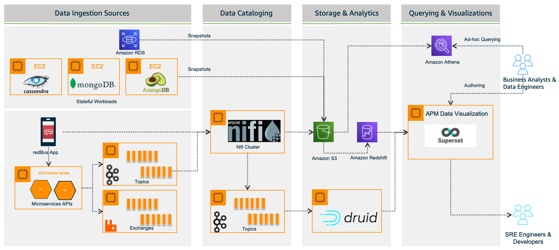
redBus relies heavily on making data-driven decisions at every level, from its traveler journey tracking, forecasting demand during high traffic, identifying and addressing bottlenecks in their bus operators signup process, and more. As redBus’s business started growing in terms of the number of cities and countries they operated in and the number of bus operators and travelers using the service in each city, the amount of incoming data also increased. The need to access and analyze the data in one place required them to build their own data platform, as shown in the following diagram.

redBus data platform 1.0

In the following sections, we look at each component in more detail.

Data ingestion sources

With the data platform 1.0, the data is ingested from various sources:

  • Real time – The real-time data flows from redBus mobile apps, the backend microservices, and when a passenger, bus operator, or application does any operation like booking bus tickets, searching the bus inventory, uploading a KYC document, and more
  • Batch mode – Scheduled jobs fetch data from multiple persistent data stores like Amazon Relational Database Service (Amazon RDS), where the OLTP data from all its applications are stored, Apache Cassandra clusters, where the bus inventory from various operators is stored, Arango DB, where the user identity graphs are stored, and more

Data cataloging

The real-time data is ingested into their self-managed Apache Nifi clusters, an open-source data platform that is used to clean, analyze, and catalog the data with its routing capabilities before sending the data to its destination.

Storage and analytics

redBus uses the following services for its storage and analytical needs:

  • Amazon Simple Storage Service (Amazon S3), an object storage service that provides the foundation for their data lake because of its virtually unlimited scalability and higher durability. Real-time data flows from Apache Druid and data from the data stores flow at regular intervals based on the schedules.
  • Apache Druid, an OLAP-style data store (data flows via Kafka Druid data loader), which computes facts and metrics against various dimensions during the data loading process.
  • Amazon Redshift, a cloud data warehouse service that helps you analyze exabytes of data and run complex analytical queries. redBus uses Amazon Redshift to store the processed data from Amazon S3 and the aggregated data from Apache Druid.

Querying and visualization

To make redBus as data-driven as possible, they ensured that the data is accessible to their SRE engineers, data engineers, and business analysts via a visualization layer. This layer features dashboards being served using Apache SuperSet, an open-source data visualization application, and Amazon Athena, an interactive query service to analyze data in Amazon S3 using standard SQL for ad hoc querying requirements.

The challenges

Initially, redBus handled data that was being ingested at the rate of 10 million events per day. Over time, as its business started growing, so did the data volume (from gigabytes to terabytes to petabytes), data ingestion per day (from 10 million to 320 million events), and its business intelligence dashboard needs. Soon after, they started facing challenges with their self-managed Superset’s BI capabilities, and the increased operational complexities.

Limited BI capabilities

redBus encountered the following BI limitations:

  • Inability to create visualizations from multiple data sources – Superset doesn’t allow creating visualizations from multiple tables within its data exploration layer. redBus data engineers had to have the tables joined beforehand at the data source level itself. In order to create a 360-degree view for redBus’s business stakeholders, it became inconvenient for data engineers to maintain multiple tables supporting the visualization layer.
  • No global filter for visuals in a dashboard – A global or primary filter across visuals in a dashboard is not supported in Superset. For example, consider there are visuals like Sales Wins by Region, YTD Revenue Realized by Region, Sales Pipeline by Region, and more in a dashboard, and a filter Region is added to the dashboard with values like EMEA, APAC, and US. The filter Region will only apply to one of the visuals, not the entire dashboard. However, dashboard users expected filtering across the dashboard.
  • Not a business-user friendly tool – Superset is highly developer centric when it comes to customization. For example, if a redBus business analyst had to customize a timed refresh that automatically re-queries every slice on a dashboard according to a pre-set value, then the analyst has to update the dashboard’s JSON metadata field. Therefore, having knowledge of JSON and its syntax is mandatory for doing any customization on the visuals or dashboard.

Increased operational cost

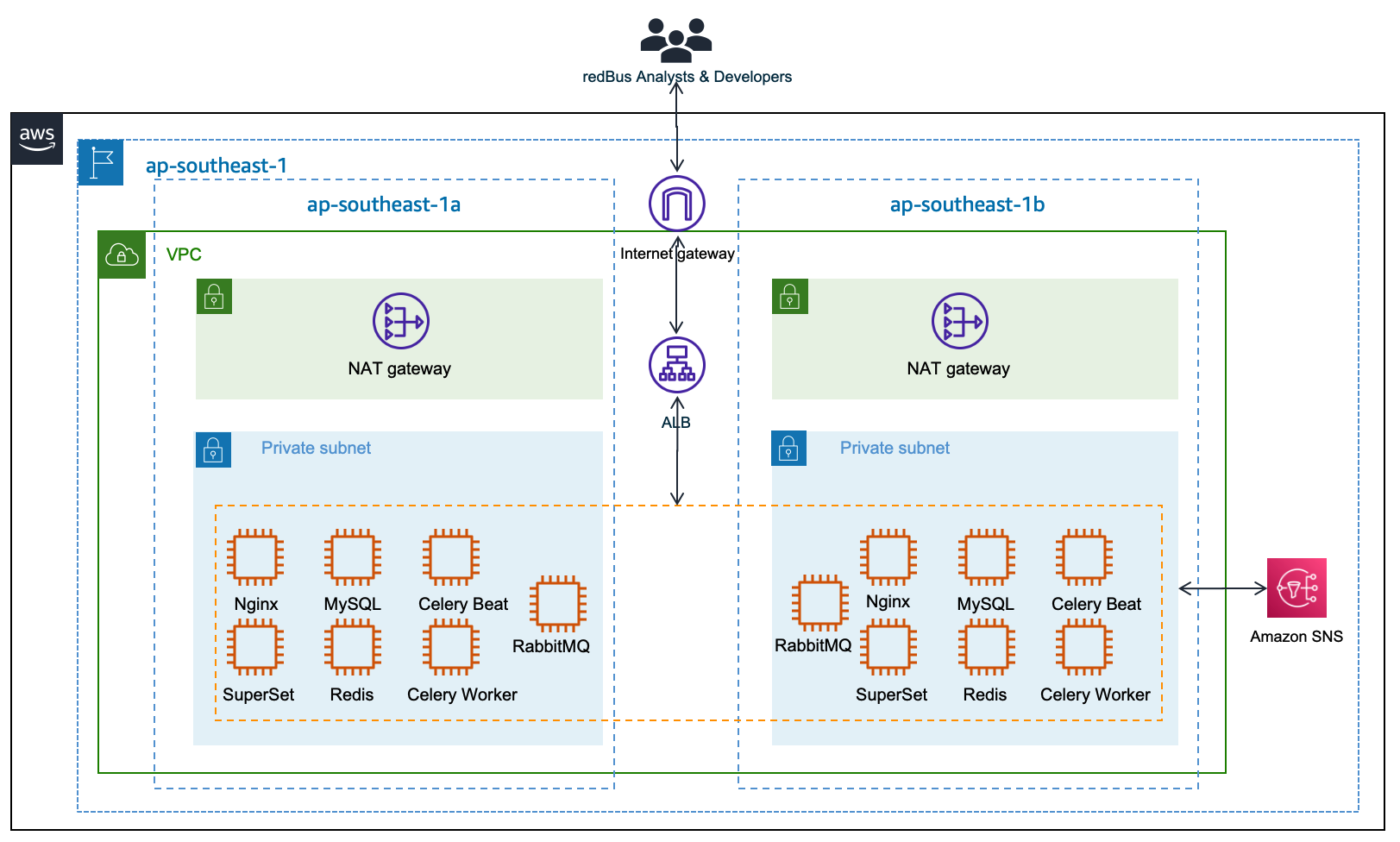
Although Superset is open source, which means there are no licensing costs, it also means there is more effort in maintaining all the components required for it to function as an enterprise-grade BI tool. redBus has deployed and maintained a web server (Nginx) fronted by an Application Load Balancer to do the load balancing; a metadata database server (MySQL) where Superset stores its internal information like users, slices, and dashboard definitions; an asynchronous task queue (Celery) for supporting long-running queries; a message broker (RabbitMQ); and a distributed caching server (Redis) for caching the results, charting data, and more on Amazon Elastic Compute Cloud (Amazon EC2) instances. The following diagram illustrates this architecture.

Apache Superset Deploment at redBus

redBus’s DevOps team had to do the heavy lifting of provisioning the infrastructure, taking backups, scaling the components manually as needed, upgrading the components individually, and more. It also required a Python web developer to be around for making the configurational changes so all the components work together seamlessly. All these manual operations increased the total cost of ownership for redBus.

Journey towards QuickSight

redBus started exploring BI solutions primarily around a couple of its dashboarding requirements:

  • BI dashboards for business stakeholders and analysts, where the data is sourced via Amazon S3 and Amazon Redshift.
  • A real-time application performance monitoring (APM) dashboard to help their SRE engineers and developers identify the root cause of an issue in their microservices deployment so they can fix the issues before they affect their customer’s experience. In this case, the data is sourced via Druid.

QuickSight fit into most of redBus’s BI dashboard requirements, and in no time their data platform team started with a proof of concept (POC) for a couple of their complex dashboards. At the end of the POC, which spanned a month’s time, the team shared their findings.

First, QuickSight is rich in BI capabilities, including the following:

  • It’s a self-service BI solution with drag-and-drop features that could help redBus analysts comfortably use it without any coding efforts.
  • Visualizations from multiple data sources in a single dashboard could help redBus business stakeholders get a 360-degree view of sales, forecasting, and insights in a single pane of glass.
  • Cascading filters across visuals and across sheets in a dashboard are much-needed features for redBus’s BI requirements.
  • QuickSight offers Excel-like visuals—tables with calculations, pivot tables with cell grouping, and styling are attractive for the viewers.
  • The Super-fast, Parallel, In-memory Calculation Engine (SPICE) in QuickSight could help redBus scale to hundreds of thousands of users, who can all simultaneously perform fast interactive analysis across a wide variety of AWS data sources.
  • Off-the-shelf ML insights and forecasting at no additional cost would allow redBus’s data science team to focus on ML models besides sales forecasting and similar models.
  • Built-in row-level security (RLS) could allow redBus to grant filtered access for their viewers. For example, redBus has many business analysts who manage different countries. With RLS, each business analyst only sees data related to their assigned country within a single dashboard.
  • redBus uses OneLogin as its identity provider, which supports Security Assertion Markup Language 2.0 (SAML 2.0). With the help of identity federation and single sign-on support from QuickSight, redBus could provide a simple onboarding flow for their QuickSight users.
  • QuickSight offers built-in alerts and email notification capabilities.

Secondly, QuickSight is a fully managed, cloud-native, serverless BI service offering from AWS, with the following features:

  • redBus engineers don’t need to focus on the heavy lifting of provisioning, scaling, and maintaining their BI solution on EC2 instances.
  • QuickSight offers native integration with AWS services like Amazon Redshift, Amazon S3, and Athena, and other popular frameworks like Presto, Snowflake, Teradata, and more. QuickSight connects to most of the data sources that redBus already has except Apache Druid, because native integration with Druid was not available as of December 2022. For a complete list of the supported data sources, see Supported data sources.

The outcome

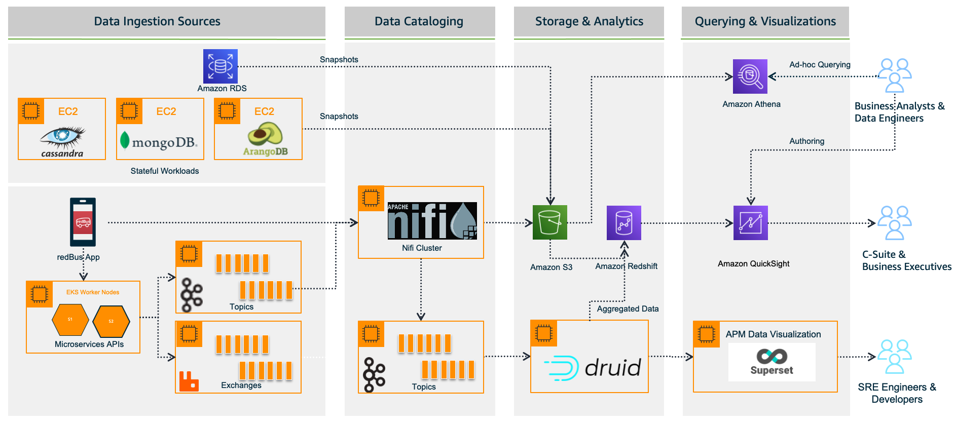
Considering all the rich features and lower total cost of ownership, redBus chose QuickSight for their BI dashboard requirements. With QuickSight, redBus’s data engineers have built a number of dashboards in no time to give insights from petabytes of data to business stakeholders and analysts. The redBus data highway evolved to bring business intelligence to a much wider audience in their organization, with better performance and faster time-to-value. As of November 2022, it combines QuickSight for business users and Superset for real-time APM dashboards (at the time of writing, QuickSight doesn’t offer a native connector to Druid), as shown in the following diagram.

redBus data platform 2.0

Sales anomaly detection dashboard

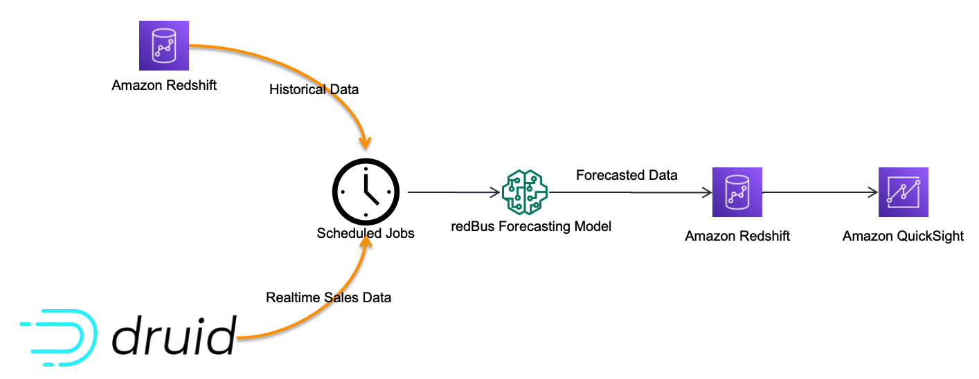
Although there are many dashboards that redBus deployed to production, sales anomaly detection is one of the interesting dashboards that redBus built. It uses redBus’s proprietary sales forecasting model, which in turn is sourced by historical sales data from Amazon Redshift tables and real-time sales data from Druid tables, as shown in the following figure.

Sales anomaly detection data flow

At regular intervals, the scheduled jobs feed the redBus forecasting model with real-time and historical sales data, and then the forecasted data is pushed into an Amazon Redshift table. The sales anomaly detection dashboard in QuickSight is served by the resultant Amazon Redshift table.

The following is one of the visuals from the sales anomaly detection dashboard. It’s built using a line chart representing hourly actual sales, predicted sales, and an alert threshold for a time series for a particular business cohort in redBus.

Sales and Predicted Sales for a particular cohort

In this visual, each bar represents the number of sales anomalies triggered at a particular point in the time series.

redBus’s analysts could further drill down to the sales details and anomalies at the minute level, as shown in the following diagram. This drill-down feature comes out of the box with QuickSight.

Drill-Down Chart - Sales and Predicted Sales for a particular cohort

For more details on adding drill-downs to QuickSight dashboard visuals, see Adding drill-downs to visual data in Amazon QuickSight.

Apart from the visuals, it has become one of viewers’ favorite dashboards at redBus due to the following notable features:

  • Because filtering across visuals is an out-of-the-box feature in QuickSight, a timestamp-based filter is added to the dashboard. This helps in filtering multiple visuals in the dashboard in a single click.
  • URL actions configured on the visuals help the viewers navigate to the context-sensitive in-house applications.
  • Email alerts configured on KPIs and Gauge visuals help the viewers get notifications on time.

Next steps

Apart from building new dashboards for their BI dashboard needs, redBus is taking the following next steps:

  • Exploring QuickSight Embedded Analytics for a couple of their application requirements to accelerate time to insights for users with in-context data visuals, interactive dashboards, and more directly within applications
  • Exploring QuickSight Q, which could enable their business stakeholders to ask questions in natural language and receive accurate answers with relevant visualizations that can help them gain insights from the data
  • Building a unified dashboarding solution using QuickSight covering all their data sources as integrations become available

Conclusion

In this post, we showed you how redBus built its data platform using various AWS services and Apache frameworks, the challenges the platform went through (especially in their BI dashboard requirements and challenges while scaling), and how they used QuickSight and lowered the total cost of ownership.

To know more about engineering at redBus, check out their medium blog posts. To learn more about what is happening in QuickSight or if you have any questions, reach out to the QuickSight Community, which is very active and offers several resources.


About the Authors


Author: Girish Chidanand
Girish Kumar Chidananda
works as a Senior Engineering Manager – Data Engineering at redBus, where he has been building various data engineering applications and components for redBus for the last 5 years. Prior to starting his journey in the IT industry, he worked as a Mechanical and Control systems engineer in various organizations, and he holds an MS degree in Fluid Power Engineering from University of Bath.


Author: Kayalvizhi Kandasamy
Kayalvizhi Kandasamy
works with digital-native companies to support their innovation. As a Senior Solutions Architect (APAC) at Amazon Web Services, she uses her experience to help people bring their ideas to life, focusing primarily on microservice architectures and cloud-native solutions using AWS services. Outside of work, she likes playing chess and is a FIDE rated chess player. She also coaches her daughters the art of playing chess, and prepares them for various chess tournaments.

Automate data lineage on Amazon MWAA with OpenLineage

Post Syndicated from Stephen Said original https://aws.amazon.com/blogs/big-data/automate-data-lineage-on-amazon-mwaa-with-openlineage/

In modern data architectures, datasets are combined across an organization using a variety of purpose-built services to unlock insights. As a result, data governance becomes a key component for data consumers and producers to know that their data-driven decisions are based on trusted and accurate datasets. One aspect of data governance is data lineage, which captures the flow of data as it goes through various systems and allows consumers to understand how a dataset was derived.

In order to capture data lineage consistently across various analytical services, you need to use a common lineage model and a robust job orchestration that is able to tie together diverse data flows. One possible solution is the open-source OpenLineage project. It provides a technology-agnostic metadata model for capturing data lineage and integrates with widely used tools. For job orchestration, it integrates with Apache Airflow, which you can run on AWS conveniently through the managed service Amazon Managed Workflows for Apache Airflow (Amazon MWAA). OpenLineage provides a plugin for Apache Airflow that extracts data lineage from Directed Acyclic Graphs (DAGs).

In this post, we show how to get started with data lineage on AWS using OpenLineage. We provide a step-by-step configuration guide for the openlineage-airflow plugin on Amazon MWAA. Additionally, we share an AWS Cloud Development Kit (AWS CDK) project that deploys a pre-configured demo environment for evaluating and experiencing OpenLineage first-hand.

OpenLineage on Apache Airflow

In the following example, Airflow turns OLTP data into a star schema on Amazon Redshift Serverless.

After staging and preparing source data from Amazon Simple Storage Service (Amazon S3), fact and dimension tables are eventually created. For this, Airflow orchestrates the execution of SQL statements that create and populate tables on Redshift Serverless.

Overview on DAGs in Amazon MWAA

The openlineage-airflow plugin collects metadata about creation of datasets and dependencies between them. This allows us to move from a jobs-centric approach of Airflow to a datasets-centric approach, improving the observability of workflows.

The following screenshot shows parts of the captured lineage for the previous example. It’s displayed in Marquez, an open-source metadata service for collection and visualization of data lineage with support for the OpenLineage standard. In Marquez, you can analyze the upstream datasets and transformations that eventually create the user dimension table on the right.

Data lineage graph in marquez

The example in this post is based on SQL and Amazon Redshift. OpenLineage also supports other transformation engines and data stores such as Apache Spark and dbt.

Solution overview

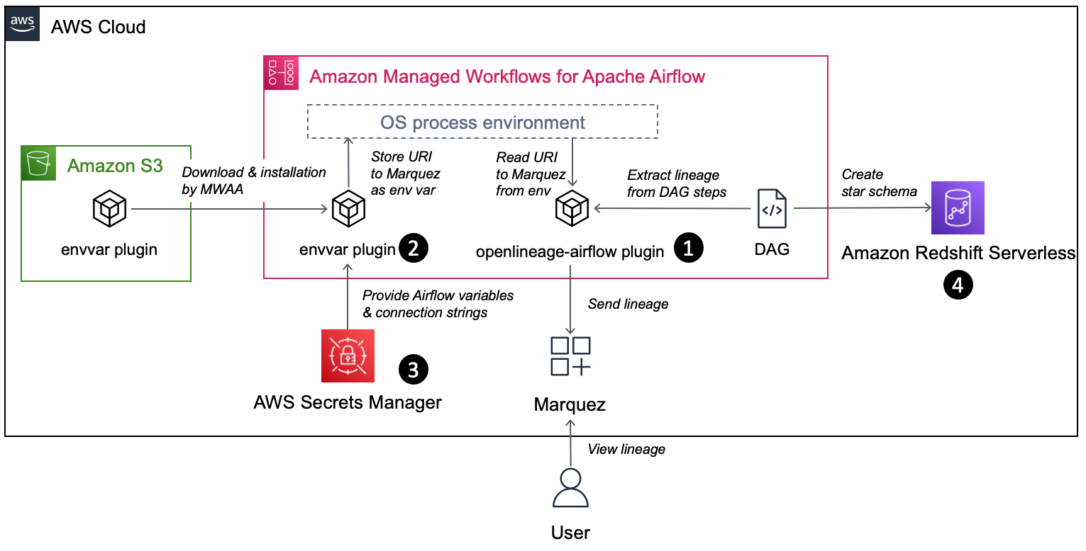
The following diagram shows the AWS setup required to capture data lineage using OpenLineage.

Solution overview

The workflow includes the following components:

  1. The openlineage-airflow plugin is configured on Airflow as a lineage backend. Metadata about the DAG runs is passed by Airflow core to the plugin, which converts it into OpenLineage format and sends it to an external metadata store. In our demo setup, we use Marquez as the metadata store.
  2. The openlineage-airflow plugin receives its configuration from environment variables. To populate these variables on Amazon MWAA, a custom Airflow plugin is used. First, the plugin reads source values from AWS Secrets Manager. Then, it creates environment variables.
  3. Secrets Manager is configured as a secrets backend. Typically, this type of configuration is stored in Airflow’s native metadata database. However, this approach has limitations. For instance, in case of multiple Airflow environments, you need to track and store credentials across multiple environments, and updating credentials requires you to update all the environments. With a secrets backend, you can centralize configuration.
  4. For demo purposes, we collect data lineage from a data pipeline, which creates a star schema in Redshift Serverless.

In the following sections, we walk you through the steps for end-to-end configuration.

Install the openlineage-airflow plugin

Specify the following dependency in the requirements.txt file of the Amazon MWAA environment. Note that the latest Airflow version currently available on Amazon MWAA is 2.4.3; for this post, use the compatible version 0.19.2 of the plugin:

openlineage-airflow==0.19.2

For more details on installing Python dependencies on Amazon MWAA, refer to Installing Python dependencies.

For Airflow < 2.3, configure the plugin’s lineage backend through the following configuration overrides on the Amazon MWAA environment and load it immediately at Airflow start by disabling lazy load of plugins:

AirflowConfigurationOptions:
    core.lazy_load_plugins: False
    lineage.backend: openlineage.lineage_backend.OpenLineageBackend

For more information on configuration overrides, refer to Configuration options overview.

Configure the Secrets Manager backend with Amazon MWAA

Using Secrets Manager as a secrets backend for Amazon MWAA is straightforward. First, provide the execution role of Amazon MWAA with read permission to Secrets Manager. You can use the following policy template as a starting point:

{
  "Version": "2012-10-17",
  "Statement": [
    {
      "Effect": "Allow",
      "Action": [
        "secretsmanager:GetResourcePolicy",
        "secretsmanager:GetSecretValue",
        "secretsmanager:DescribeSecret",
        "secretsmanager:ListSecretVersionIds"
      ],
      "Resource": "arn:aws:secretsmanager:AWS_REGION:<YOUR_ACCOUNT_ID>:secret:"
    },
    {
      "Effect": "Allow",
      "Action": "secretsmanager:ListSecrets",
      "Resource": ""
    }
  ]
}

Second, configure Secrets Manager as a backend in Amazon MWAA through the following configuration overrides:

AirflowConfigurationOptions:
secrets.backend: airflow.contrib.secrets.aws_secrets_manager.SecretsManagerBackend
secrets.backend_kwargs: '{"connections_prefix" : "airflow/connections", "variables_prefix" : "airflow/variables"}'

For more information configuring a secrets backend in Amazon MWAA, refer to Configuring an Apache Airflow connection using a Secrets Manager secret and Move your Apache Airflow connections and variables to AWS Secrets Manager.

Deploy a custom envvar plugin to Amazon MWAA

Apache Airflow has a built-in plugin manager through which it can be extended with custom functionality. In our case, this functionality is to populate OpenLineage-specific environment variables based on values in Secrets Manager. Natively, Amazon MWAA allows environment variables with the prefix AIRFLOW__, but the openlineage-airflow plugin expects the prefix OPENLINEAGE__.

The following Python code is used in the plugin. We assume the file is called envvar_plugin.py:

from airflow.plugins_manager import AirflowPlugin
from airflow.models import Variable
import os

os.environ["OPENLINEAGE_URL"] = Variable.get('OPENLINEAGE_URL', default_var='')

class EnvVarPlugin(AirflowPlugin):
  name = "env_var_plugin"

Amazon MWAA has a mechanism to install a plugin through a zip archive. You zip your code, upload the archive to an S3 bucket, and pass the URL to the file to Amazon MWAA:

zip plugins.zip envvar_plugin.py

Upload plugins.zip to an S3 bucket and configure the URL in Amazon MWAA. The following screenshot shows the configuration via the Amazon MWAA console.

Configuration of a custom plugin in Amazon MWAA

For more information on installing custom plugins on Amazon MWAA, refer to Creating a custom plugin that generates runtime environment variables.

Configure connectivity between the openlineage-airflow plugin and Marquez

As a last step, store the URL to Marquez in Secrets Manager. For this, create a secret called airflow/variables/OPENLINEAGE_URL with value <protocol>://<hostname/ip>:<port> (for example, https://marquez.mysite.com:5000).

Configuration of OPENLINEAGE_URL as secret

In case you need to spin up Marquez on AWS, you have multiple options to host, including running it on Amazon Elastic Kubernetes Service (Amazon EKS) or Amazon Elastic Compute Cloud (Amazon EC2). Refer to Running Marquez on AWS or check out our infrastructure template in the next section to deploy Marquez on AWS.

Deploy with an AWS CDK-based solution template

Assuming you want to set up a demo infrastructure for all of the above in one step, you can use the following template based on the AWS CDK.

The template has the following prerequisites:

Complete the following steps to deploy the template:

  1. Clone GitHub repository and install Python dependencies. Bootstrap the AWS CDK if required.
    git clone https://github.com/aws-samples/aws-mwaa-openlineage 
    	cd aws-mwaa-openlineage
    	python3 -m venv .env && source .env/bin/activate
    	python3 -m pip install -r requirements.txt
    	cdk bootstrap

  2. Update the value for the variable EXTERNAL_IP in constants.py to your outbound IP for connecting to the internet:
    # Set variable to outbound IP for connecting to the internet.
    EXTERNAL_IP = "255.255.255.255"

    This configures security groups so that you can access Marquez but block other clients. constants.py is found in the root folder of the cloned repository.

  3. Deploy the VPC_S3 stack to provision a new VPC dedicated for this solution as well as the security groups that are used by the different components:
    cdk deploy vpc-s3

    It creates a new S3 bucket and uploads the source raw data based on the TICKIT sample database. This serves as the landing area from the OLTP database. We then need to parse the metadata of these files through an AWS Glue crawler, which facilitates the native integration between Amazon Redshift and the S3 data lake.

  4. Deploy the lineage stack to create an EC2 instance that hosts Marquez:
    cdk deploy marquez

    Access the Marquez web UI through https://{ec2.public_dns_name}:3000/. This URL is also available as part of the AWS CDK outputs for the lineage stack.

  5. Deploy the Amazon Redshift stack to create a Redshift Serverless endpoint:
    cdk deploy redshift

  6. Deploy the Amazon MWAA stack to create an Amazon MWAA environment:
    cdk deploy mwaa

    You can access the Amazon MWAA UI through the URL provided in the AWS CDK output.

Test a sample data pipeline

On Amazon MWAA, you can see an example data pipeline deployed that consists of two DAGs. It builds a star schema on top of the TICKIT sample database. One DAG is responsible for loading data from the S3 data lake into an Amazon Redshift staging layer; the second DAG loads data from the staging layer to the dimensional model.

Datamodel of star schema

Open the Amazon MWAA UI through the URL obtained in the deployment steps and launch the following DAGs: rs_source_to_staging and rs_staging_to_dm. As part of the run, the lineage metadata is sent to Marquez.

After the DAG has been run, open the Marquez URL obtained in the deployment steps. In Marquez, you can find the lineage metadata for the computed star schema and related data assets on Amazon Redshift.

Clean up

Delete the AWS CDK stacks to avoid ongoing charges for the resources that you created. Run the following command in the aws-mwaa-openlineage project directory so that all resources are undeployed:

cdk destroy --all

Summary

In this post, we showed you how to automate data lineage with OpenLineage on Amazon MWAA. As part of this, we covered how to install and configure the openlineage-airflow plugin on Amazon MWAA. Additionally, we provided a ready-to-use infrastructure template for a complete demo environment.

We encourage you to explore what else can be achieved with OpenLineage. A job orchestrator like Apache Airflow is only one piece of a data platform and not all possible data lineage can be captured on it. We recommend exploring OpenLineage’s integration with other platforms like Apache Spark or dbt. For more information, refer to Integrations.

Additionally, we recommend you visit the AWS Big Data Blog for other useful blog posts on Amazon MWAA and data governance on AWS.


About the Authors

Stephen Said is a Senior Solutions Architect and works with Digital Native Businesses. His areas of interest are data analytics, data platforms and cloud-native software engineering.

Vishwanatha Nayak is a Senior Solutions Architect at AWS. He works with large enterprise customers helping them design and build secure, cost-effective, and reliable modern data platforms using the AWS cloud. He is passionate about technology and likes sharing knowledge through blog posts and twitch sessions.

Paul Villena is an Analytics Solutions Architect with expertise in building modern data and analytics solutions to drive business value. He works with customers to help them harness the power of the cloud. His areas of interests are infrastructure-as-code, serverless technologies and coding in Python.

Enable cross-account sharing with direct IAM principals using AWS Lake Formation Tags

Post Syndicated from Aarthi Srinivasan original https://aws.amazon.com/blogs/big-data/enable-cross-account-sharing-with-direct-iam-principals-using-aws-lake-formation-tags/

With AWS Lake Formation, you can build data lakes with multiple AWS accounts in a variety of ways. For example, you could build a data mesh, implementing a centralized data governance model and decoupling data producers from the central governance. Such data lakes enable the data as an asset paradigm and unleash new possibilities with data discovery and exploration across organization-wide consumers. While enabling the power of data in decision-making across your organization, it’s also crucial to secure the data. With Lake Formation, sharing datasets across accounts only requires a few simple steps, and you can control what you share.

Lake Formation has launched Version 3 capabilities for sharing AWS Glue Data Catalog resources across accounts. When moving to Lake Formation cross-account sharing V3, you get several benefits. When moving from V1, you get more optimized usage of AWS Resource Access Manager (AWS RAM) to scale sharing of resources. When moving from V2, you get a few enhancements. First, you don’t have to maintain AWS Glue resource policies to share using LF-tags because Version 3 uses AWS RAM. Second, you can share with AWS Organizations using LF-tags. Third, you can share to individual AWS Identity and Access Management (IAM) users and roles in other accounts, thereby providing data owners control over which individuals can access their data.

Lake Formation tag-based access control (LF-TBAC) is an authorization strategy that defines permissions based on attributes called LF-tags. LF-tags are different from IAM resource tags and are associated only with Lake Formation databases, tables, and columns. LF-TBAC allows you to define the grant and revoke permissions policy by grouping Data Catalog resources, and therefore helps in scaling permissions across a large number of databases and tables. LF-tags are inherited from a database to all its tables and all the columns of each table.

Version 3 offers the following benefits:

  • True central governance with cross-account sharing to specific IAM principals in the target account
  • Ease of use in not having to maintain an AWS Glue resource policy for LF-TBAC
  • Efficient reuse of AWS RAM shares
  • Ease of use in scaling to hundreds of accounts with LF-TBAC

In this post, we illustrate the new features of cross-account sharing Version 3 in a producer-consumer scenario using TPC datasets. We walk through the setup of using LF-TBAC to share data catalog resources from the data producer account to direct IAM users in the consumer account. We also go through the steps in the receiving account to accept the shares and query the data.

Solution overview

To demonstrate the Lake Formation cross-account Version 3 features, we use the TPC datasets available at s3://aws-data-analytics-workshops/shared_datasets/tpcparquet/. The solution consists of steps in both accounts.

In account A, complete the following steps:

  1. As a data producer, register the dataset with Lake Formation and create AWS Glue Data Catalog tables.
  2. Create LF-tags and associate them with the database and tables.
  3. Grant LF-tag based permissions on resources directly to personas in consumer account B.

The following steps take place in account B:

  1. The consumer account data lake admin reviews and accepts the AWS RAM invitations.
  2. The data lake admin gives CREATE DATABASE access to the IAM user lf_business_analysts.
  3. The data lake admin creates a database for the marketing team and grants CREATE TABLE access to lf_campaign_manager.
  4. The IAM users create resource links on the shared database and tables and query them in Amazon Athena.

The producer account A has the following personas:

  • Data lake admin – Manages the data lake in the producer account
  • lf-producersteward – Manages the data and user access

The consumer account B has the following personas:

  • Data lake admin – Manages the data lake in the consumer account
  • lf-business-analysts – The business analysts in the sales team needs access to non-PII data
  • lf-campaign-manager – The manager in the marketing team needs access to data related to products and promotions

Prerequisites

You need the following prerequisites:

  • Two AWS accounts. For this demonstration of how AWS RAM invites are created and accepted, you should use two accounts that are not part of the same organization.
  • An admin IAM user in both accounts to launch the AWS CloudFormation stacks.
  • Lake Formation mode enabled in both the producer and consumer account with cross-account Version 3. For instructions, refer to Change the default permission model.

Lake Formation and AWS CloudFormation setup in account A

To keep the setup simple, we have an IAM admin registered as the data lake admin.

  1. Sign into the AWS Management Console in the us-east-1 Region.
  2. On the Lake Formation console, under Permissions in the navigation pane, choose Administrative roles and tasks.
  3. Select Choose Administrators under Datalake administrators.
  4. In the pop-up window Manage data lake administrators, under IAM users and roles, choose IAM admin user and choose Save.
  5. Choose Launch Stack to deploy the CloudFormation template:
    BDB-2063-launch-cloudformation-stack
  6. Choose Next.
  7. Provide a name for the stack and choose Next.
  8. On the next page, choose Next.
  9. Review the details on the final page and select I acknowledge that AWS CloudFormation might create IAM resources.
  10. Choose Create.

Stack creation should take about 2–3 minutes. The stack establishes the producer setup as follows:

  • Creates an Amazon Simple Storage Service (Amazon S3) data lake bucket
  • Registers the data lake bucket with Lake Formation
  • Creates an AWS Glue database and tables
  • Creates an IAM user (lf-producersteward) who will act as producer steward
  • Creates LF-tags and assigns them to the created catalog resources as specified in the following table
Database Table LF-Tag Key LF-Tag Value Resource Tagged
lftpcdb . Sensitivity Public DATABASE
lftpcdb items HasCampaign true TABLE
lftpcdb promotions HasCampaign true TABLE
lftpcdb customers table columns = "c_last_name","c_first_name","c_email_address" Sensitivity Confidential TABLECOLUMNS

Verify permissions in account A

After the CloudFormation stack launches, complete the following steps in account A:

  1. On the AWS CloudFormation console, navigate to the Outputs tab of the stack.

  1. Choose the LFProducerStewardCredentials value to navigate to the AWS Secrets Manager console.
  2. In the Secret value section, choose Retrieve secret value.
  3. Note down the secret value for the password for IAM user lf-producersteward.

You need this to log in to the console later as the user lf-producersteward.

  1. On the LakeFormation console, choose Databases on the navigation pane.
  2. Open the database lftpcdb.
  3. Verify the LF-tags on the database are created.

  1. Choose View tables and choose the items table to verify the LF-tags.

  1. Repeat the steps for the promotions and customers tables to verify the LF-tags assigned.

  1. On the Lake Formation console, under Data catalog in the navigation pane, choose Databases.
  2. Select the database lftpcdb and on the Actions menu, choose View Permissions.
  3. Verify that there are no default permissions granted on the database lftpcdb for IAMAllowedPrincipals.
  4. If you find any, select the permission and choose Revoke to revoke the permission.
  5. On the AWS Management Console, choose the AWS CloudShell icon on the top menu.

This opens AWS CloudShell in another tab of the browser. Allow a few minutes for the CloudShell environment to set up.

  1. Run the following AWS Command Line Interface (AWS CLI) command after replacing {BUCKET_NAME} with DataLakeBucket from the stack output.
aws s3 cp s3://aws-data-analytics-workshops/shared_datasets/tpcparquet/ s3://${BUCKET_NAME}/tpcparquet/  --recursive

If CloudShell isn’t available in your chosen Region, run the following AWS CLI command to copy the required dataset from your preferred AWS CLI environment as the IAM admin user.

  1. Verify that your S3 bucket has the dataset copied in it.
  2. Log out as the IAM admin user.

Grant permissions in account A

Next, we continue granting Lake Formation permissions to the dataset as a data steward within the producer account. The data steward grants the following LF-tag-based permissions to the consumer personas.

Consumer Persona LF-tag Policy
lf-business-analysts Sensitivity=Public
lf-campaign-manager HasCampaign=true
  1. Log in to account A as user lf-producersteward, using the password you noted from Secrets Manager earlier.
  2. On the Lake Formation console, under Permissions in the navigation pane, choose Data Lake permissions.
  3. Choose Grant.
  4. Under Principals, select External accounts.
  5. Provide the ARN of the IAM user in the consumer account (arn:aws:iam::<accountB_id>:user/lf-business-analysts) and press Enter.

  1. Under LF_Tags or catalog resources, select Resources matched by LF-Tags.
  2. Choose Add LF-Tag to add a new key-value pair.
  3. For the key, choose Sensitivity and for the value, choose Public.
  4. Under Database permissions, select Describe, and under Table permissions, select Select and Describe.

  1. Choose Grant to apply the permissions.
  2. On the Lake Formation console, under Permissions in the navigation pane, choose Data Lake permissions.
  3. Choose Grant.
  4. Under Principals, select External accounts.
  5. Provide the ARN of the IAM user in the consumer account (arn:aws:iam::<accountB_id>:user/lf-campaign-manager) and press Enter.
  6. Under LF_Tags or catalog resources, select Resources matched by LF-Tags.
  7. Choose Add LF-Tag to add a new key-value pair.
  8. For the key, choose HasCampaign and for the value, choose true.

  1. Under Database permissions, select Describe, and under Table permissions, select Select and Describe.
  2. Choose Grant to apply the permissions.
  3.  Verify on the Data lake permissions tab that the permissions you have granted show up correctly.

AWS CloudFormation setup in account B

Complete the following steps in the consumer account:

  1. Log in as an IAM admin user in account B and launch the CloudFormation stack:
    BDB-2063-launch-cloudformation-stack
  2. Choose Next.
  3. Provide a name for the stack, then choose Next.
  4. On the next page, choose Next.
  5. Review the details on the final page and select I acknowledge that AWS CloudFormation might create IAM resources.
  6. Choose Create.

Stack creation should take about 2–3 minutes. The stack sets up the following resources in account B:

  • IAM users datalakeadmin1, lf-business-analysts, and lf-campaign-manager, with relevant IAM and Lake Formation permissions
  • A database called db_for_shared_tables with Create_Table permissions to the lf-campaign-manager user
  • An S3 bucket named lfblog-athenaresults-<your-accountB-id>-us-east-1 with ListBucket and write permissions to lf-business-analysts and lf-campaign-manager

Note down the stack output details.

Accept resource shares in account B

After you launch the CloudFormation stack, complete the following steps in account B:

  1. On the CloudFormation stack Outputs tab, choose the link for DataLakeAdminCredentials.

This takes you to the Secrets Manager console.

  1. On the Secrets Manager console, choose Retrieve secret value and copy the password for DataLakeAdmin user.
  2. Use the ConsoleIAMLoginURL value from the CloudFormation template output to log in to account B with the data lake admin user name datalakeadmin1 and the password you copied from Secrets Manager.
  3. Open the AWS RAM console in another browser tab.
  4. In the navigation pane, under Shared with me, choose Resource shares to view the pending invitations.

You should see two resource share invitations from the producer account A: one for database-level share and one for table-level share.

  1. Choose each resource share link, review the details, and choose Accept.

After you accept the invitations, the status of the resource shares changes from Active from Pending.

Grant permissions in account B

To grant permissions in account B, complete the following steps:

  1. On the Lake Formation console, under Permissions on the navigation pane, choose Administrative roles and tasks.

  1. Under Database creators, choose Grant.

  1. Under IAM users and roles, choose lf-business-analysts.
  2. For Catalog permissions, select Create database.
  3. Choose Grant.
  4. Log out of the console as the data lake admin user.

Query the shared datasets as consumer users

To validate the lf-business-analysts user’s data access, perform the following steps:

  1. Log in to the console as lf-business-analysts, using the credentials noted from the CloudFormation stack output.
  2. On the Lake Formation console, under Data catalog in the navigation pane, choose Databases.

  1. Select the database lftpcdb and on the Actions menu, choose Create resource link.

  1. Under Resource link name, enter rl_lftpcdb.
  2. Choose Create.
  3. After the resource link is created, select the resource link and choose View tables.

You can now see the four tables in the shared database.

  1. Open the Athena console in another browser tab and choose the lfblog-athenaresults-<your-accountB-id>-us-east-1 bucket as the query results location.
  2. Verify data access using the following query (for more information, refer to Running SQL queries using Amazon Athena):
Select * from rl_lftpcdb.customers limit 10;

The following screenshot shows the query output.

Notice that account A shared the database lftpcdb to account B using the LF-tag expression Sensitivity=Public. Columns c_first_name, c_last_name, and c_email_address in table customers were overwritten with Sensitivity=Confidential. Therefore, these three columns are not visible to user lf-business-analysts.

You can preview the other tables from the database similarly to see the available columns and data.

  1. Log out of the console as lf-business-analysts.

Now we can validate the lf-campaign-manager user’s data access.

  1. Log in to the console as lf-campaign-manager using the credentials noted from the CloudFormation stack output.
  2. On the Lake Formation console, under Data catalog in the navigation pane, choose Databases.
  3. Verify that you can see the database db_for_shared_tables shared by the data lake admin.

  1. Under Data catalog in the navigation pane, choose Tables.

You should be able to see the two tables shared from account A using the LF-tag expression HasCampaign=true. The two tables show the Owner account ID as account A.

Because lf-campaign-manager received table level shares, this user will create table-level resource links for querying in Athena.

  1. Select the promotions table, and on the Actions menu, choose Create resource link.

  1. For Resource link name, enter rl_promotions.

  1. Under Database, choose db_for_shared_tables for the database to contain the resource link.
  2. Choose Create.
  3. Repeat the table resource link creation for the other table items.

Notice that the resource links show account B as owner, whereas the actual tables show account A as the owner.

  1. Open the Athena console in another browser tab and choose the lfblog-athenaresults-<your-accountB-id>-us-east-1 bucket as the query results location.
  2. 11. Query the tables using the resource links.

As shown in the following screenshot, all columns of both tables are accessible to lf-campaign-manager.

In summary, you have seen how LF-tags are used to share a database and select tables from one account to another account’s IAM users.

Clean up

To avoid incurring charges on the AWS resources created in this post, you can perform the following steps.

First, clean up resources in account A:

  1. Empty the S3 bucket created for this post by deleting the downloaded objects from your S3 bucket.
  2. Delete the CloudFormation stack.

This deletes the S3 bucket, custom IAM roles, policies, and the LF database, tables, and permissions.

  1. You may choose to undo the Lake Formation settings also and add IAM access back from the Lake Formation console Settings page.

Now complete the following steps in account B:

  1. Empty the S3 bucket lfblog-athenaresults-<your-accountB-id>-us-east-1 used as the Athena query results location.
  2. Revoke permission to lf-business-analysts as database creator.
  3. Delete the CloudFormation stack.

This deletes the IAM users, S3 bucket, Lake Formation database db_for_shared_tables, resource links, and all the permissions from Lake Formation.

If there are any resource links and permissions left, delete them manually in Lake Formation from both accounts.

Conclusion

In this post, we illustrated the benefits of using Lake Formation cross-account sharing Version 3 using LF-tags to direct IAM principals and how to receive the shared tables in the consumer account. We used a two-account scenario in which a data producer account shares a database and specific tables to individual IAM users in another account using LF-tags. In the receiving account, we showed the role played by a data lake admin vs. the receiving IAM users. We also illustrated how to overwrite column tags to mask and share PII data.

With Version 3 of cross-account sharing features, Lake Formation makes possible more modern data mesh models, where a producer can directly share to an IAM principal in another account, instead of the entire account. Data mesh implementation becomes easier for data administrators and data platform owners because they can easily scale to hundreds of consumer accounts using the LF-tags based sharing to organizational units or IDs.

We encourage you to upgrade your Lake Formation cross-account sharing to Version 3 and benefit from the enhancements. For more details, see Updating cross-account data sharing version settings.


About the authors

Aarthi Srinivasan is a Senior Big Data Architect with AWS Lake Formation. She likes building data lake solutions for AWS customers and partners. When not on the keyboard, she explores the latest science and technology trends and spends time with her family.

Srividya Parthasarathy is a Senior Big Data Architect on the AWS Lake Formation team. She enjoys building analytics and data mesh solutions on AWS and sharing them with the community.

How to encrypt sensitive caller voice input in Amazon Lex

Post Syndicated from Herbert Guerrero original https://aws.amazon.com/blogs/security/how-to-encrypt-sensitive-caller-authentication-voice-input-in-amazon-lex/

In the telecommunications industry, sensitive authentication and user data are typically received through mobile voice and keypads, and companies are responsible for protecting the data obtained through these channels. The increasing use of voice-driven interactive voice response (IVR) has resulted in a need to provide solutions that can protect user data that is gathered from mobile voice inputs. In this blog post, you’ll see how to protect a caller’s sensitive voice data that was captured through Amazon Lex by using data encryption implemented through AWS Lambda functions. The solution described in this post helps you to protect customer data received through voice channels from inadvertent or unknown access. The solution also includes decryption capabilities, which give an authorized administrator or operator the ability to decrypt user data from a Lambda console.

Solution overview

To demonstrate the IVR solution described in this post, a caller speaks two sensitive pieces of data—credit card number and zip code—from an Amazon Connect contact flow. The spoken values are encrypted and returned to the contact flow to be stored in contact attributes. The encrypted ciphertext is retained as a contact attribute for decryption purposes. Amazon CloudWatch Logs is enabled in the contact flow, but only the encrypted values are logged in log streams.

For this solution, conversation logs for this Amazon Lex bot are not enabled. An operator with assigned AWS Identity and Access Management (IAM) permissions can monitor the logged encrypted entries from CloudWatch Logs. For more information, see Working with log groups and log streams in the Amazon CloudWatch Logs User Guide.

Solution architecture

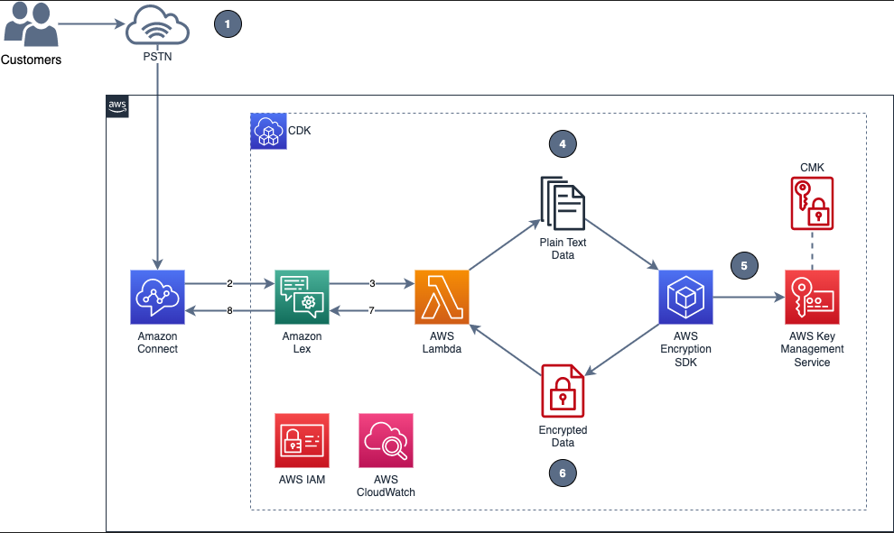
Figure 1 shows the overview of the solution described in this blog post.

Figure 1: Example of solution architecture

Figure 1: Example of solution architecture

Figure 1 shows the following high-level steps of the solution, and the number labels correspond to the following steps.

  1. A caller places an inbound call.
  2. An Amazon Connect contact flow leverages a Get customer input block, backed by an Amazon Lex bot, to prompt the caller for numerical data.
  3. The Amazon Lex bot invokes the Lambda function dev-encryption-core-EncryptFn.
  4. The Lambda function uses the AWS Encryption SDK to encrypt the caller’s plain text data.
  5. The AWS Encryption SDK obtains encryption keys from AWS Key Management Service (AWS KMS).
  6. The caller’s data is encrypted by using the AWS KMS keys obtained from AWS KMS.
  7. The Lambda function appends the encrypted data to the Amazon Lex bot session attributes.
  8. Amazon Lex returns the fully encrypted data back to Amazon Connect.

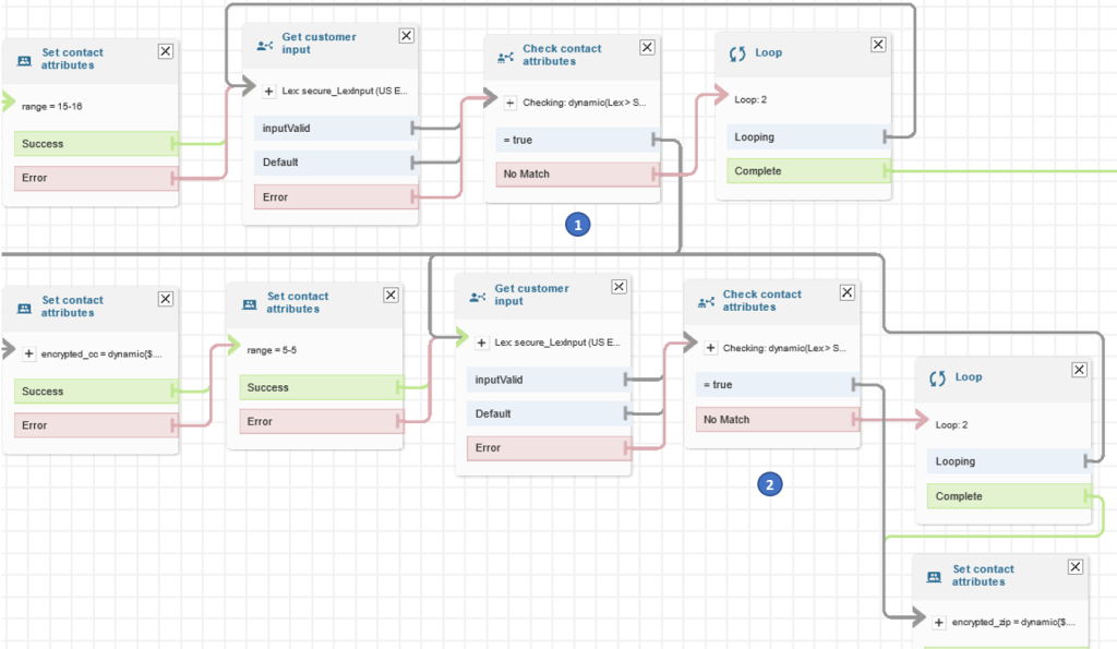
Overview of a contact flow

Figure 2: Contact flow captures input values using Amazon Lex and returns their encrypted values

Figure 2: Contact flow captures input values using Amazon Lex and returns their encrypted values

Figure 2 shows an overview of the contact flow, which has two main steps:

  1. The first numerical data (in this example, an encrypted credit card number value) is stored in contact attributes.
  2. The second numerical data (in this example, an encrypted zip code value) is stored in contact attributes.

Prerequisites

This solution uses the following AWS services:

The following need to be installed in your local machine:

To implement the solution in this post, you first need the Amazon Connect instance prerequisite in place.

To set up the Amazon Connect instance (if none exists)

  1. Create an Amazon Connect instance with a claimed phone number and a configured Amazon Connect user linked to a basic routing profile. For more information about setting up a contact center, see Set up your contact center in the Amazon Connect Administrator Guide.
  2. Assign the CallCenterManager or Admin security profile to an Amazon Connect user.
  3. In the newly created Amazon Connect instance, under the Overview section, find the access URL with the format
    https://<aliasname>.awsapps.com/connect/login

    • Make note of the access URL, which you will use later to log in to the Amazon Connect Dashboard.
  4. Log in to your Amazon Connect instance with a Connect user that has Admin or CallCenterManager permissions.

Solution procedures

This solution includes the following procedures:

  1. Clone the project or download the solution zip file.
  2. Create AWS resources needed for encryption and decryption.
  3. Configure the Amazon Lex bot in Amazon Connect.
  4. Create the contact flow in Amazon Connect.
  5. Validate the solution.
  6. Decrypt the collected data.

To clone or download the solution

  • Log in to the GitHub repo.
  • Clone or download the solution files to your local machine.

The downloaded file contains the artifacts needed for the deployment.

To create AWS resources needed for encryption and decryption

  1. From the command line, change directory to the project’s root directory.
  2. Run npm install.
  3. Run npm run build to transpile TypeScript to JavaScript and package code and its dependencies before deploying to AWS.
  4. Run cdk deploy CoreStack.

To configure the Amazon Lex bot in your Amazon Connect instance

  1. In the Amazon Connect console, choose Contact flows and scroll to the Amazon Lex section.
    Figure 3: Select Contact flows

    Figure 3: Select Contact flows

  2. From the Bot menu, select secure_LexInput(Classic). Then select +Add Amazon Lex Bot.
    Figure 4: Configure the Amazon Lex bot to Amazon Connect

    Figure 4: Configure the Amazon Lex bot to Amazon Connect

To import contact flow into Amazon Connect

  1. In the Amazon Connect console, choose Overview, and then choose Login as administrator.
  2. From the Routing menu on the left side, choose Contact flows to show the list of contact flows.
  3. Choose Create Contact flow.
  4. Choose the arrow to the right of the Save button and choose Import flow (beta). This imports the contact flow that you previously downloaded in the procedure To clone or download the solution.

    The contact flow already has the Amazon Lex bot configured.

    Figure 5: Select Import flow (beta)

    Figure 5: Select Import flow (beta)

  5. In the upper right corner of the contact flow, choose Save, and then choose OK to save the changes.
  6. Choose Publish to make the contact flow ready for use during the validation steps.
  7. (Optional) Claim a phone number (if none is available), using the following steps:
    1. In the Connect Dashboard, on the navigation menu, choose Channels, and then choose Phone numbers.
    2. On the right side of the page, choose Claim a number.
    3. Select the DID (Direct Inward Dialing) tab. Use the drop-down arrow to choose your country/region. When numbers are returned, choose one.
    4. Write down the phone number. You call it later in this post.
  8. (Optional) On the Edit Phone number page, in the Description box, you can type a note if desired.
  9. To assign the contact flow to your claimed phone number, for Contact flow / IVR, choose the drop-down arrow, and then choose Secure_Lex_Input.
  10. Choose Save.
    Figure 6: Under Contact flow / IVR, select the imported contact flow

    Figure 6: Under Contact flow / IVR, select the imported contact flow

For more information, see Set up phone numbers for your contact center in the Amazon Connect Administrator Guide.

To validate the solution

  1. Dial the test phone number to go through the voice prompt flow.
  2. When prompted, speak a 16-digit credit card number (you have a maximum of two retries), then speak a 5-digit zip code (also a maximum of two retries).
  3. After you complete your test call, review the log streams in Amazon CloudWatch Logs to confirm that the digits that you entered are now encrypted and stored as a contact attribute. The two entered values zipcode and creditcard are stored in contact attributes. Both are encrypted.
    Figure 7: Sample log showing encrypted values for zipcode and creditcard

    Figure 7: Sample log showing encrypted values for zipcode and creditcard

  4. Log in to your Amazon Connect Dashboard as a Supervisor. The URL is provided after the connect instance has been created. In the navigation menu, choose Contact search.
    Figure 8: Choose Contact search to look for the call information

    Figure 8: Choose Contact search to look for the call information

  5. Locate your inbound call on the Contact search list. Note that it can take up to 60 seconds for data to appear in the Contact search list.
  6. Select the Contact ID for your call.
    Figure 9: The Contact search showing the contact details for your test call

    Figure 9: The Contact search showing the contact details for your test call

  7. Copy the encrypted values for creditcard and zipcode and make note of them; you will use these values in the next procedure.
    Figure 10: Contact attributes stored in a contact flow are registered as part of the contact details

    Figure 10: Contact attributes stored in a contact flow are registered as part of the contact details

To decrypt the collected data

  1. In the AWS Lambda console, choose Functions.
  2. Use the Search bar to look for the dev-encryption-core-DecryptFn Lambda function, and then select the name link to open it.
  3. Under folder encryption-master, open the test folder. Under the tab \events, locate the file decrypt.json.
  4. Use the following steps to create a sample test event in the console by using the contents from decrypt.json. For more details, see Testing Lambda functions in the console.
    1. Choose the down arrow on the right side of Test.
    2. Choose Configure test event.
    3. Choose Create new test event.
    4. For Event name, enter decryptTest.
    5. Paste the contents from decrypt.json.
      {
          "Details": {
              "Parameters": {
                  "encrypted": "<encrypted-value-here>"
              }
          }
      }

    6. Choose Save.
  5. Use the encrypted values saved in the Validate a solution procedure and replace the ones in the recently created test event.
    Figure 11: Replace the creditcard or zipCode values with the ones from the Contact Search page

    Figure 11: Replace the creditcard or zipCode values with the ones from the Contact Search page

  6. Choose Test. The output from the test shows the values decrypted by the Lambda function. This is shown in Figure 12 under the Execution result tab.
    Figure 12: Result from the decryption operation

    Figure 12: Result from the decryption operation

Note: Make sure that only the appropriate authorized administrator or operator, application, or AWS service is able to invoke the decryption Lambda function.

You have now successfully implemented the solution by encrypting and decrypting the voice input of your test call, which you collected through Amazon Lex.

Cleanup

To avoid incurring future charges, follow these steps to clean up the deployed resources that you created when implementing this solution.

To delete the Amazon Connect instance

  1. In the Amazon Connect console, under Instance alias, select the name of the Amazon Connect instance, and choose Delete.
  2. When prompted, type the name of the instance, and then choose Delete.

To delete the Amazon Lex bot

  1. In the Amazon Lex console, choose the bot that you created in the To configure the Amazon Lex bot procedure.
  2. Choose Delete, and then choose Continue.

To delete the AWS CloudFormation stack

  1. In the AWS CloudFormation console, on the Stacks page, select the stack you created in the procedure To create AWS resources needed for encryption and decryption.
  2. In the stack details pane, choose Delete.
  3. Choose Delete stack when prompted. This deletes the Amazon S3 bucket, IAM roles and AWS Lambda functions you created for testing. This will also schedule a deletion date on the AWS KMS key.

Conclusion

In this post, you learned how an Amazon Connect contact flow can collect voice inputs from a caller by using Amazon Lex, and how you can encrypt these inputs by using your own AWS KMS key. This solution can help improve the security of voice input that is collected through Amazon Connect. For cost information, see the Amazon Connect pricing page.

For more information, see the blog post Creating a secure IVR solution with Amazon Connect and the topic Encrypt customer input (using OpenSSL) in the Amazon Connect Administrator Guide. As previously mentioned, the increasing use of voice-driven IVR has resulted in a need to provide solutions that can protect user data gathered from mobile voice inputs.

Additional resources include the AWS Lambda Developer Guide, the Amazon Lex Developer Guide, the Amazon Connect Administrator Guide, the AWS Nodejs SDK, and the AWS SDK for Python (Boto3).

If you need help with setting up this solution, you can get assistance from AWS Professional Services. You can also seek assistance from Amazon Connect partners available worldwide.

 
If you have feedback about this post, submit comments in the Comments section below. If you have questions about this post, contact AWS Support.

Want more AWS Security news? Follow us on Twitter.

Herbert Guerrero

Herbert Guerrero

Herbert is a Senior Proserve Consultant for Connect. He enjoys designing and developing high-usability and scalable solutions. Understanding success criteria helps Herbert work backwards and deliver well-architected solutions. His engineering background informs the way he engages with customers’ mental models of what their solutions should look like.

Ed Valdez

Ed Valdez

Ed is a Specialty Consultant with Amazon Web Services. As a software development professional with over 23 years of experience, he specializes on designing and delivering customer-centric solutions within the contact center domain.

How BookMyShow saved 80% in costs by migrating to an AWS modern data architecture

Post Syndicated from Mahesh Vandi Chalil original https://aws.amazon.com/blogs/big-data/how-bookmyshow-saved-80-in-costs-by-migrating-to-an-aws-modern-data-architecture/

This is a guest post co-authored by Mahesh Vandi Chalil, Chief Technology Officer of BookMyShow.

BookMyShow (BMS), a leading entertainment company in India, provides an online ticketing platform for movies, plays, concerts, and sporting events. Selling up to 200 million tickets on an annual run rate basis (pre-COVID) to customers in India, Sri Lanka, Singapore, Indonesia, and the Middle East, BookMyShow also offers an online media streaming service and end-to-end management for virtual and on-ground entertainment experiences across all genres.

The pandemic gave BMS the opportunity to migrate and modernize our 15-year-old analytics solution to a modern data architecture on AWS. This architecture is modern, secure, governed, and cost-optimized architecture, with the ability to scale to petabytes. BMS migrated and modernized from on-premises and other cloud platforms to AWS in just four months. This project was run in parallel with our application migration project and achieved 90% cost savings in storage and 80% cost savings in analytics spend.

The BMS analytics platform caters to business needs for sales and marketing, finance, and business partners (e.g., cinemas and event owners), and provides application functionality for audience, personalization, pricing, and data science teams. The prior analytics solution had multiple copies of data, for a total of over 40 TB, with approximately 80 TB of data in other cloud storage. Data was stored on‑premises and in the cloud in various data stores. Growing organically, the teams had the freedom to choose their technology stack for individual projects, which led to the proliferation of various tools, technology, and practices. Individual teams for personalization, audience, data engineering, data science, and analytics used a variety of products for ingestion, data processing, and visualization.

This post discusses BMS’s migration and modernization journey, and how BMS, AWS, and AWS Partner Minfy Technologies team worked together to successfully complete the migration in four months and saving costs. The migration tenets using the AWS modern data architecture made the project a huge success.

Challenges in the prior analytics platform

  • Varied Technology: Multiple teams used various products, languages, and versions of software.
  • Larger Migration Project: Because the analytics modernization was a parallel project with application migration, planning was crucial in order to consider the changes in core applications and project timelines.
  • Resources: Experienced resource churn from the application migration project, and had very little documentation of current systems.
  • Data : Had multiple copies of data and no single source of truth; each data store provided a view for the business unit.
  • Ingestion Pipelines: Complex data pipelines moved data across various data stores at varied frequencies. We had multiple approaches in place to ingest data to Cloudera, via over 100 Kafka consumers from transaction systems and MQTT(Message Queue Telemetry Transport messaging protocol) for clickstreams, stored procedures, and Spark jobs. We had approximately 100 jobs for data ingestion across Spark, Alteryx, Beam, NiFi, and more.
  • Hadoop Clusters: Large dedicated hardware on which the Hadoop clusters were configured incurring fixed costs. On-premises Cloudera setup catered to most of the data engineering, audience, and personalization batch processing workloads. Teams had their implementation of HBase and Hive for our audience and personalization applications.
  • Data warehouse: The data engineering team used TiDB as their on-premises data warehouse. However, each consumer team had their own perspective of data needed for analysis. As this siloed architecture evolved, it resulted in expensive storage and operational costs to maintain these separate environments.
  • Analytics Database: The analytics team used data sourced from other transactional systems and denormalized data. The team had their own extract, transform, and load (ETL) pipeline, using Alteryx with a visualization tool.

Migration tenets followed which led to project success:

  • Prioritize by business functionality.
  • Apply best practices when building a modern data architecture from Day 1.
  • Move only required data, canonicalize the data, and store it in the most optimal format in the target. Remove data redundancy as much possible. Mark scope for optimization for the future when changes are intrusive.
  • Build the data architecture while keeping data formats, volumes, governance, and security in mind.
  • Simplify ELT and processing jobs by categorizing the jobs as rehosted, rewritten, and retired. Finalize canonical data format, transformation, enrichment, compression, and storage format as Parquet.
  • Rehost machine learning (ML) jobs that were critical for business.
  • Work backward to achieve our goals, and clear roadblocks and alter decisions to move forward.
  • Use serverless options as a first option and pay per use. Assess the cost and effort for rearchitecting to select the right approach. Execute a proof of concept to validate this for each component and service.

Strategies applied to succeed in this migration:

  • Team – We created a unified team with people from data engineering, analytics, and data science as part of the analytics migration project. Site reliability engineering (SRE) and application teams were involved when critical decisions were needed regarding data or timeline for alignment. The analytics, data engineering, and data science teams spent considerable time planning, understanding the code, and iteratively looking at the existing data sources, data pipelines, and processing jobs. AWS team with partner team from Minfy Technologies helped BMS arrive at a migration plan after a proof of concept for each of the components in data ingestion, data processing, data warehouse, ML, and analytics dashboards.
  • Workshops – The AWS team conducted a series of workshops and immersion days, and coached the BMS team on the technology and best practices to deploy the analytics services. The AWS team helped BMS explore the configuration and benefits of the migration approach for each scenario (data migration, data pipeline, data processing, visualization, and machine learning) via proof-of-concepts (POCs). The team captured the changes required in the existing code for migration. BMS team also got acquainted with the following AWS services:
  • Proof of concept – The BMS team, with help from the partner and AWS team, implemented multiple proofs of concept to validate the migration approach:
    • Performed batch processing of Spark jobs in Amazon EMR, in which we checked the runtime, required code changes, and cost.
    • Ran clickstream analysis jobs in Amazon EMR, testing the end-to-end pipeline. Team conducted proofs of concept on AWS IoT Core for MQTT protocol and streaming to Amazon S3.
    • Migrated ML models to Amazon SageMaker and orchestrated with Amazon MWAA.
    • Created sample QuickSight reports and dashboards, in which features and time to build were assessed.
    • Configured for key scenarios for Amazon Redshift, in which time for loading data, query performance, and cost were assessed.
  • Effort vs. cost analysis – Team performed the following assessments:
    • Compared the ingestion pipelines, the difference in data structure in each store, the basis of the current business need for the data source, the activity for preprocessing the data before migration, data migration to Amazon S3, and change data capture (CDC) from the migrated applications in AWS.
    • Assessed the effort to migrate approximately 200 jobs, determined which jobs were redundant or need improvement from a functional perspective, and completed a migration list for the target state. The modernization of the MQTT workflow code to serverless was time-consuming, decided to rehost on Amazon Elastic Compute Cloud (Amazon EC2) and modernization to Amazon Kinesis in to the next phase.
    • Reviewed over 400 reports and dashboards, prioritized development in phases, and reassessed business user needs.

AWS cloud services chosen for proposed architecture:

  • Data lake – We used Amazon S3 as the data lake to store the single truth of information for all raw and processed data, thereby reducing the copies of data storage and storage costs.
  • Ingestion – Because we had multiple sources of truth in the current architecture, we arrived at a common structure before migration to Amazon S3, and existing pipelines were modified to do preprocessing. These one-time preprocessing jobs were run in Cloudera, because the source data was on-premises, and on Amazon EMR for data in the cloud. We designed new data pipelines for ingestion from transactional systems on the AWS cloud using AWS Glue ETL.
  • Processing – Processing jobs were segregated based on runtime into two categories: batch and near-real time. Batch processes were further divided into transient Amazon EMR clusters with varying runtimes and Hadoop application requirements like HBase. Near-real-time jobs were provisioned in an Amazon EMR permanent cluster for clickstream analytics, and a data pipeline from transactional systems. We adopted a serverless approach using AWS Glue ETL for new data pipelines from transactional systems on the AWS cloud.
  • Data warehouse – We chose Amazon Redshift as our data warehouse, and planned on how the data would be distributed based on query patterns.
  • Visualization – We built the reports in Amazon QuickSight in phases and prioritized them based on business demand. We discussed with business users their current needs and identified the immediate reports required. We defined the phases of report and dashboard creation and built the reports in Amazon QuickSight. We plan to use embedded reports for external users in the future.
  • Machine learning – Custom ML models were deployed on Amazon SageMaker. Existing Airflow DAGs were migrated to Amazon MWAA.
  • Governance, security, and compliance – Governance with Amazon Lake Formation was adopted from Day 1. We configured the AWS Glue Data Catalog to reference data used as sources and targets. We had to comply to Payment Card Industry (PCI) guidelines because payment information was in the data lake, so we ensured the necessary security policies.

Solution overview

BMS modern data architecture

The following diagram illustrates our modern data architecture.

The architecture includes the following components:

  1. Source systems – These include the following:
    • Data from transactional systems stored in MariaDB (booking and transactions).
    • User interaction clickstream data via Kafka consumers to DataOps MariaDB.
    • Members and seat allocation information from MongoDB.
    • SQL Server for specific offers and payment information.
  2. Data pipeline – Spark jobs on an Amazon EMR permanent cluster process the clickstream data from Kafka clusters.
  3. Data lake – Data from source systems was stored in their respective Amazon S3 buckets, with prefixes for optimized data querying. For Amazon S3, we followed a hierarchy to store raw, summarized, and team or service-related data in different parent folders as per the source and type of data. Lifecycle polices were added to logs and temp folders of different services as per teams’ requirements.
  4. Data processing – Transient Amazon EMR clusters are used for processing data into a curated format for the audience, personalization, and analytics teams. Small file merger jobs merge the clickstream data to a larger file size, which saved costs for one-time queries.
  5. Governance – AWS Lake Formation enables the usage of AWS Glue crawlers to capture the schema of data stored in the data lake and version changes in the schema. The Data Catalog and security policy in AWS Lake Formation enable access to data for roles and users in Amazon Redshift, Amazon Athena, Amazon QuickSight, and data science jobs. AWS Glue ETL jobs load the processed data to Amazon Redshift at scheduled intervals.
  6. Queries – The analytics team used Amazon Athena to perform one-time queries raised from business teams on the data lake. Because report development is in phases, Amazon Athena was used for exporting data.
  7. Data warehouse – Amazon Redshift was used as the data warehouse, where the reports for the sales teams, management, and third parties (i.e., theaters and events) are processed and stored for quick retrieval. Views to analyze the total sales, movie sale trends, member behavior, and payment modes are configured here. We use materialized views for denormalized tables, different schemas for metadata, and transactional and behavior data.
  8. Reports – We used Amazon QuickSight reports for various business, marketing, and product use cases.
  9. Machine learning – Some of the models deployed on Amazon SageMaker are as follows:
    • Content popularity – Decides the recommended content for users.
    • Live event popularity – Calculates the popularity of live entertainment events in different regions.
    • Trending searches – Identifies trending searches across regions.

Walkthrough

Migration execution steps

We standardized tools, services, and processes for data engineering, analytics, and data science:

  • Data lake
    • Identified the source data to be migrated from Archival DB, BigQuery, TiDB, and the analytics database.
    • Built a canonical data model that catered to multiple business teams and reduced the copies of data, and therefore storage and operational costs. Modified existing jobs to facilitate migration to a canonical format.
    • Identified the source systems, capacity required, anticipated growth, owners, and access requirements.
    • Ran the bulk data migration to Amazon S3 from various sources.
  • Ingestion
    • Transaction systems – Retained the existing Kafka queues and consumers.
    • Clickstream data – Successfully conducted a proof of concept to use AWS IoT Core for MQTT protocol. But because we needed to make changes in the application to publish to AWS IoT Core, we decided to implement it as part of mobile application modernization at a later time. We decided to rehost the MQTT server on Amazon EC2.
  • Processing
  • Listed the data pipelines relevant to business and migrated them with minimal modification.
  • Categorized workloads into critical jobs, redundant jobs, or jobs that can be optimized:
    • Spark jobs were migrated to Amazon EMR.
    • HBase jobs were migrated to Amazon EMR with HBase.
    • Metadata stored in Hive-based jobs were modified to use the AWS Glue Data Catalog.
    • NiFi jobs were simplified and rewritten in Spark run in Amazon EMR.
  • Amazon EMR clusters were configured one persistent cluster for streaming the clickstream and personalization workloads. We used multiple transient clusters for running all other Spark ETL or processing jobs. We used Spot Instances for task nodes to save costs. We optimized data storage with specific jobs to merge small files and compressed file format conversions.
  • AWS Glue crawlers identified new data in Amazon S3. AWS Glue ETL jobs transformed and uploaded processed data to the Amazon Redshift data warehouse.
  • Datawarehouse
    • Defined the data warehouse schema by categorizing the critical reports required by the business, keeping in mind the workload and reports required in future.
    • Defined the staging area for incremental data loaded into Amazon Redshift, materialized views, and tuning the queries based on usage. The transaction and primary metadata are stored in Amazon Redshift to cater to all data analysis and reporting requirements. We created materialized views and denormalized tables in Amazon Redshift to use as data sources for Amazon QuickSight dashboards and segmentation jobs, respectively.
    • Optimally used the Amazon Redshift cluster by loading last two years data in Amazon Redshift, and used Amazon Redshift Spectrum to query historical data through external tables. This helped balance the usage and cost of the Amazon Redshift cluster.
  • Visualization
    • Amazon QuickSight dashboards were created for the sales and marketing team in Phase 1:
      • Sales summary report – An executive summary dashboard to get an overview of sales across the country by region, city, movie, theatre, genre, and more.
      • Live entertainment – A dedicated report for live entertainment vertical events.
      • Coupons – A report for coupons purchased and redeemed.
      • BookASmile – A dashboard to analyze the data for BookASmile, a charity initiative.
  • Machine learning
    • Listed the ML workloads to be migrated based on current business needs.
    • Priority ML processing jobs were deployed on Amazon EMR. Models were modified to use Amazon S3 as source and target, and new APIs were exposed to use the functionality. ML models were deployed on Amazon SageMaker for movies, live event clickstream analysis, and personalization.
    • Existing artifacts in Airflow orchestration were migrated to Amazon MWAA.
  • Security
    • AWS Lake Formation was the foundation of the data lake, with the AWS Glue Data Catalog as the foundation for the central catalog for the data stored in Amazon S3. This provided access to the data by various functionalities, including the audience, personalization, analytics, and data science teams.
    • Personally identifiable information (PII) and payment data was stored in the data lake and data warehouse, so we had to comply to PCI guidelines. Encryption of data at rest and in transit was considered and configured in each service level (Amazon S3, AWS Glue Data Catalog, Amazon EMR, AWS Glue, Amazon Redshift, and QuickSight). Clear roles, responsibilities, and access permissions for different user groups and privileges were listed and configured in AWS Identity and Access Management (IAM) and individual services.
    • Existing single sign-on (SSO) integration with Microsoft Active Directory was used for Amazon QuickSight user access.
  • Automation
    • We used AWS CloudFormation for the creation and modification of all the core and analytics services.
    • AWS Step Functions was used to orchestrate Spark jobs on Amazon EMR.
    • Scheduled jobs were configured in AWS Glue for uploading data in Amazon Redshift based on business needs.
    • Monitoring of the analytics services was done using Amazon CloudWatch metrics, and right-sizing of instances and configuration was achieved. Spark job performance on Amazon EMR was analyzed using the native Spark logs and Spark user interface (UI).
    • Lifecycle policies were applied to the data lake to optimize the data storage costs over time.

Benefits of a modern data architecture

A modern data architecture offered us the following benefits:

  • Scalability – We moved from a fixed infrastructure to the minimal infrastructure required, with configuration to scale on demand. Services like Amazon EMR and Amazon Redshift enable us to do this with just a few clicks.
  • Agility – We use purpose-built managed services instead of reinventing the wheel. Automation and monitoring were key considerations, which enable us to make changes quickly.
  • Serverless – Adoption of serverless services like Amazon S3, AWS Glue, Amazon Athena, AWS Step Functions, and AWS Lambda support us when our business has sudden spikes with new movies or events launched.
  • Cost savings – Our storage size was reduced by 90%. Our overall spend on analytics and ML was reduced by 80%.

Conclusion

In this post, we showed you how a modern data architecture on AWS helped BMS to easily share data across organizational boundaries. This allowed BMS to make decisions with speed and agility at scale; ensure compliance via unified data access, security, and governance; and to scale systems at a low cost without compromising performance. Working with the AWS and Minfy Technologies teams helped BMS choose the correct technology services and complete the migration in four months. BMS achieved the scalability and cost-optimization goals with this updated architecture, which has set the stage for innovation using graph databases and enhanced our ML projects to improve customer experience.


About the Authors

Mahesh Vandi Chalil is Chief Technology Officer at BookMyShow, India’s leading entertainment destination. Mahesh has over two decades of global experience, passionate about building scalable products that delight customers while keeping innovation as the top goal motivating his team to constantly aspire for these. Mahesh invests his energies in creating and nurturing the next generation of technology leaders and entrepreneurs, both within the organization and outside of it. A proud husband and father of two daughters and plays cricket during his leisure time.

Priya Jathar is a Solutions Architect working in Digital Native Business segment at AWS. She has more two decades of IT experience, with expertise in Application Development, Database, and Analytics. She is a builder who enjoys innovating with new technologies to achieve business goals. Currently helping customers Migrate, Modernise, and Innovate in Cloud. In her free time she likes to paint, and hone her gardening and cooking skills.

Vatsal Shah is a Senior Solutions Architect at AWS based out of Mumbai, India. He has more than nine years of industry experience, including leadership roles in product engineering, SRE, and cloud architecture. He currently focuses on enabling large startups to streamline their cloud operations and help them scale on the cloud. He also specializes in AI and Machine Learning use cases.

Code conversion from Greenplum to Amazon Redshift: Handling arrays, dates, and regular expressions

Post Syndicated from Jagrit Shrestha original https://aws.amazon.com/blogs/big-data/code-conversion-from-greenplum-to-amazon-redshift-handling-arrays-dates-and-regular-expressions/

Amazon Redshift is a fully managed service for data lakes, data analytics, and data warehouses for startups, medium enterprises, and large enterprises. Amazon Redshift is used by tens of thousands of businesses around the globe for modernizing their data analytics platform.

Greenplum is an open-source, massively parallel database used for analytics, mostly for on-premises infrastructure. Greenplum is based on the PostgreSQL database engine.

Many customers have found migration to Amazon Redshift from Greenplum an attractive option instead of managing on-premises Greenplum for the following reasons:

Even though both Greenplum and Amazon Redshift use the open-source PostgreSQL database engine, migration still requires a lot of planning and manual intervention. This post covers the key functions and considerations while performing code conversion from Greenplum to Amazon Redshift. It is focused on the migration of procedures, functions, and views.

Solution overview

AWS Database Migration Service (AWS DMS) and the AWS Schema Conversion Tool (AWS SCT) can migrate most of the objects in a heterogeneous database migration from Greenplum to Amazon Redshift. But there are some situations where code conversion teams encounter errors and warnings for views, procedures, and functions while creating them in Amazon Redshift. To address this type of situation, manual conversion of the code is required.

The posts focuses on how to handle the following while migrating from Greenplum to Amazon Redshift:

  • Arrays
  • Dates and timestamps
  • Regular expressions (regex)

Please note that for this post, we use Greenplum 4.3 and Amazon Redshift PostgreSQL 8.2.

Working with array functions

The AWS SCT doesn’t convert array functions while migrating from Greenplum or PostgreSQL to Amazon Redshift. Developers need to extensively convert those functions manually. This post outlines the most common array functions:

  • ARRAY_UPPER
  • JSON_EXTACT_ARRAY_ELEMENT_TEXT and JSON_ARRAY_LENGTH
  • UNNEST ()
  • STRING_AGG()
  • ANY ARRAY()

ARRAY_UPPER()

This function returns the upper bound of an array. It can be used to extract the nth element from an array in PostgreSQL or Greenplum.

The Greenplum code is as follows:

With temp1 as
(
Select 'John' as FirstName, 'Smith' as LastName ,
array['"111-222-3333"','"101-201-3001"','"XXX-YYY-ZZZZ"','NULL'] as PhoneNumbers
union all
Select 'Bob' as FirstName, 'Haris' as LastName ,
array['222-333-4444','201-301-4001','AAA-BBB-CCCC'] as PhoneNumbers
union all
Select 'Mary' as FirstName, 'Jane' as LastName ,
array['333-444-5555','301-401-3001','DDD-EEE-FFFF'] as PhoneNumbers
)
Select Firstname, PhoneNumbers[ARRAY_UPPER(PhoneNumbers,1)]

There is no function to extract an element from an array in Amazon Redshift; however, there are two JSON functions that can be used for this purpose:

  • JSON_EXTRACT_ARRAY_ELEMENT_TEXT() – Returns a JSON array element in the outermost array of a JSON string
  • JSON_ARRAY_LENGTH() – Returns the number of elements in the outer array of a JSON string

See the following code:

With temp1 as
(
Select 'John' as FirstName, 'Smith' as LastName ,
array['"111-222-3333"','"101-201-3001"','"XXX-YYY-ZZZZ"'] as PhoneNumbers
union all
Select 'Bob' as FirstName, 'Haris' as LastName ,
array['"222-333-4444"','"201-301-4001"','"AAA-BBB-CCCC"'] as PhoneNumbers
union all
Select 'Mary' as FirstName, 'Jane' as LastName ,
array['"333-444-5555"','"301-401-3001"','"DDD-EEE-FFFF"'] as PhoneNumbers
)

Select
FirstName
,('['+array_to_string(phoneNumbers,',')+']') as JSONConvertedField
,JSON_EXTRACT_ARRAY_ELEMENT_TEXT
(
'['+array_to_string(phoneNumbers,',')+']'
,JSON_ARRAY_LENGTH('['+array_to_string(phoneNumbers,',')+']')-1
) as LastElementFromArray
from temp1

UNNEST()

UNNEST() is PostgreSQL’s system function for semi-structured data, expanding an array, or a combination of arrays to a set of rows. It is introduced to improve the database performance of thousands or records for inserts, updates, and deletes.

You can use UNNEST() for basic array, multiple arrays, and multiple arrays with different lengths.

Some of Amazon Redshift functions used to unnest arrays are split_part, json_extract_path_text, json_array_length, and json_extract_array_element_text.

In Greenplum, the UNNEST function is used to expand an array to a set of rows:

Select ‘A’,unnest(array([1,2])

Output
A 1
A 2

with temp1 as
(
Select 'John' as FirstName, 'Smith' as LastName ,
'111-222-3333' as Mobilephone,'101-201-3001' as HomePhone
union all
Select 'Bob' as FirstName, 'Haris' as LastName ,
'222-333-4444' as Mobilephone,'201-301-4001' as HomePhone
union all
Select 'Mary' as FirstName, 'Jane' as LastName ,
'333-444-5555' as Mobilephone,'301-401-3001' as HomePhone
)

select
FirstName
,LastName
,unnest(array[‘Mobile’::text,’HomePhone’::text]) as PhoneType
,unnest(array[MobilePhone::text,HomePhone::text]) as PhoneNumber
from
temp1
order by 1,2,3

Amazon Redshift doesn’t support the UNNEST function; you can use the following workaround:

with temp1 as
(
Select 'John' as FirstName, 'Smith' as LastName ,
'111-222-3333' as Mobilephone,'101-201-3001' as HomePhone
union all
Select 'Bob' as FirstName, 'Haris' as LastName ,
'222-333-4444' as Mobilephone,'201-301-4001' as HomePhone
union all
Select 'Mary' as FirstName, 'Jane' as LastName ,
'333-444-5555' as Mobilephone,'301-401-3001' as HomePhone
),
ns as
(
Select row_number() over(order by 1) as n from pg_tables
)

Select
FirstName
,LastName
,split_part('Mobile,Home',',',ns.n::int) as PhoneType
,split_part(MobilePhone|| '&&' || HomePhone, '&&', ns.n::int) as PhoneNumber
from
temp1, ns
where
ns.n<=regexp_count('Mobile,Home',',')+1
order by 1,2,3

When the element of array is in the form of array itself, use the JSON_EXTRACT_ARRAY_ELEMENT_TEXT() function and JSON_ARRAY_LENGTH:

with ns as
(
Select row_number() over(order by 1) as n from pg_tables
)

Select JSON_EXTRACT_ARRAY_ELEMENT_TEXT('["arrayelement1","arrayelement2"]',ns.n-1)
from ns
where
ns.n<=JSON_ARRAY_LENGTH('["arrayelement1","arrayelement2"]')

STRING_AGG()

The STRING_AGG() function is an aggregate function that concatenates a list of strings and places a separator between them. The function doesn’t add the separator at the end of the string. See the following code:

STRING_AGG ( expression, separator [order_by_clause] )

The Greenplum code is as follows:

with temp1 as
(
Select 'Finance'::text as Dept, 'John'::text as FirstName, 'Smith'::text as LastName
union all
Select 'Finance'::text as Dept, 'John'::text as FirstName, 'Doe'::text as LastName
union all
Select 'Finance'::text as Dept, 'Mary'::text as FirstName, 'Jane'::text as LastName
union all
Select 'Marketing'::text as Dept, 'Bob'::text as FirstName, 'Smith'::text as LastName
union all
Select 'Marketing'::text as Dept, 'Steve'::text as FirstName, 'Smith'::text as LastName
union all
Select 'Account'::text as Dept, 'Phil'::text as FirstName, 'Adams'::text as LastName
union all
Select 'Account'::text as Dept, 'Jim'::text as FirstName, 'Smith'::text as LastName
)
Select dept,STRING_AGG(FirstName||' '||LastName,' ; ') as Employees from temp1 group by dept order by 1

The Amazon Redshift equivalent for the STRING_AGG() function is LISTAGG(). This aggregate function orders the rows for that group according to the ORDER BY expression, then concatenates the values into a single string:

LISTAGG(expression, separator [order_by_clause])

See the following code:

Create temporary Table temp1 as
(
Select 'Finance'::text as Dept, 'John'::text as FirstName, 'Smith'::text as LastName
union all
Select 'Finance'::text as Dept, 'John'::text as FirstName, 'Doe'::text as LastName
union all
Select 'Finance'::text as Dept, 'Mary'::text as FirstName, 'Jane'::text as LastName
union all
Select 'Marketing'::text as Dept, 'Bob'::text as FirstName, 'Smith'::text as LastName
union all
Select 'Marketing'::text as Dept, 'Steve'::text as FirstName, 'Smith'::text as LastName
union all
Select 'Account'::text as Dept, 'Phil'::text as FirstName, 'Adams'::text as LastName
union all
Select 'Account'::text as Dept, 'Jim'::text as FirstName, 'Smith'::text as LastName
)

Select dept,LISTAGG(FirstName||' '||LastName,' ; ') as Employees from temp1
group by dept
order by 1

ANY ARRAY()

The PostgreSQL ANY ARRAY() function evaluates and compare the left-hand expression to each element in array:

Select * from temp1 where DeptName = ANY ARRAY('10-F','20-F','30-F')

In Amazon Redshift, the evaluation can be achieved with an IN operator:

Select * from temp1 where DeptName IN ('10-F','20-F','30-F')

Working with date functions

In this section, we discuss calculating the difference between date_part for Greenplum and datediff for Amazon Redshift.

When the application needs to calculate the difference between the subfields of dates for Greenplum, it uses the function date_part, which allows you to retrieve subfields such as year, month, week, and day. In the following example queries, we calculate the number of completion_days by calculating the difference between originated_date and eco_date.

To calculate the difference between the subfields of the date, Amazon Redshift has the function datediff. The following queries show an example of how to calculate the completion_days as the difference between eco_date and orginated_date. DATEDIFF determines the number of date part boundaries that are crossed between the two expressions.

We compare the Greenplum and Amazon Redshift queries as follows:

  • Difference by year

The following Greenplum query returns 1 year between 2009-01-01 and 2009-12-31:

SELECT date_part(‘year’, TIMESTAMP ‘2009-01-01’) - date_part(‘year’, 2008-12-31’) as year;

The following Amazon Redshift query returns 1 year between 2009-01-01 and 2009-12-31:

SELECT datediff (year, ‘2008-12-31’ , ‘2009-01-01’ ) as year;
  • Difference by month

The following Greenplum query returns 1 month between 2009-01-01 and 2008-12-31:

SELECT (date_part(‘year’, ‘2009-01-01’ :: date) - date_part(‘year’, ‘2008-12-31’ :: date)) * 12 +<br />(date_part(‘month’, ‘2009-01-01’) - date_part(‘month’, ‘2008-12-31’ :: date)) as month;

The following Amazon Redshift query returns 1 month between 2009-01-01 and 2008-12-31:

SELECT datediff( month, ‘2008-12-31’ , ‘2009-01-01’ ) as month;
  • Difference by week

The following Greenplum query returns 0 weeks between 2009-01-01 and 2009-12-31:

SELECT date_part(‘week’, timestamp ‘2009-01-01’ ) - date_part(‘week’, timestamp ‘2008-12-31’) as week;

The following Amazon Redshift query returns 0 weeks between 2009-01-01 and 2009-12-31:

SELECT datediff( week, ‘2008-12-31’ , ‘2009-01-01’ ) as week;
  • Difference by day

The following Greenplum query returns 1 day:

SELECT date_part ('day', '2009-01-01 24:00:00' :: timestamp - '2008-12-31 24:00:00 :: timestamp) as day;

The following Amazon Redshift query returns 1 day:

SELECT datediff (day, ‘2008-12-31’, ‘2009-01-01’) as day;
  • Difference by hour

The following Greenplum query returns 1 hour:

SELECT date_part(‘hour’, ‘2009-01-01 22:56:10’ :: timestamp - ‘2008-12-31 21:54:55' :: timestamp)

The following Amazon Redshift query returns 1 hour:

SELECT datediff (hour, ‘2009-01-01 21:56:10’, ‘2009-01-01’ ) as hour;
  • Difference by minute

The following Greenplum query returns 3 minutes:

SELECT date_part(‘minute’, ‘2009-01-01 22:56:10’ :: timestamp - ‘2009-01-01 21:53:10’ :: timestamp) as minutes;

The following Amazon Redshift query returns 1 minute:

SELECT datediff(minute, ‘2009-01-01 21:56:10’, ‘2009-01-01 21:57:55’) as minute;
  • Difference by second

The following Greenplum query returns 40 seconds:

SELECT date_part(‘second’, ‘2009-01-01 22:56:50’ :: timestamp - ‘2009-01-01 21:53:10’ : : timestamp) as seconds;

The following Amazon Redshift query returns 45 seconds:

SELECT datediff(second, ‘2009-01-01 21:56:10’, ‘2009-01-01- 21:56:55’) as seconds;

Now let’s look at how we use Amazon Redshift to calculate days and weeks in seconds.

The following Amazon Redshift query displays 2 days:

SELECT datediff(second, ‘2008-12-30 21:56:10’, ‘2009-01-01- 21:56:55’)/(60*60*24) as days;

The following Amazon Redshift query displays 9 weeks:

SELECT datediff(second, ‘2008-10-30 21:56:10’, ‘2009-01-01- 21:56:55’)/(60*60*24*7) as weeks;

For Greenplum, the date subfields need to be in single quotes, whereas for Amazon Redshift, we can use date subfields such as year, month, week, day, minute, second without quotes. For Greenplum, we have to subtract the subfield from one part to another part, whereas for Amazon Redshift we can use commas to separate the two dates.

Extract ISOYEAR from date

ISOYEAR 8601 is a week-numbering year. It begins with the Monday of the week containing the 4th of January. So for the date of early January or late December, the ISO year may be different from the Gregorian year. ISO year has 52 or 53 full weeks (364 or 371 days). The extra week is called a leap week; a year with such a week is called a leap year.

The following Greenplum query displays the ISOYEAR 2020:

SELECT extract (ISOYEAR from ‘2019-12-30’ :: date) as ISOYEARS;

The following Amazon Redshift query displays the ISOYEAR 2020:

SELECT to_char(‘2019-12-30’ :: date, ‘IYYYY’) as ISOYEARS;

Function to generate_series()

Greenplum has adopted the PostgreSQL function generate_series(). But the generate_series function works differently with Amazon Redshift while retrieving records from the table because it’s a leader node-only function.

To display a series of numbers in Amazon Redshift, run the following query on the leader node. In this example, it displays 10 rows, numbered 1–10:

SELECT generate_series(1,10);

To display a series of days for a given date, use the following query. It extracts the day from the given date and subtracts 1, to display a series of numbers from 0–6:

SELECT generate_series(0, extract(day from date ‘2009-01-07’) :: int -1);

But for the queries fetching the record from the table, joining with another table’s row, and processing data at the compute node, it doesn’t work, and generates an error message with Invalid Operation. The following code is an example of a SQL statement that works for Greenplum but fails for Amazon Redshift:

SELECT column_1,
FROM table_1t1
JOIN table_2 t2
ON t2.code = t1.code
CROSS JOIN generate_series(1,12) gen(fiscal_month)
WHERE condition_1

For Amazon Redshift, the solution is to create a table to store the series data, and rewrite the code as follows:

SELECT column1,
FROM table_t1 t1
JOIN table_t2 t2
ON t2.code = t1.code
CROSS JOIN (select “number” as fiscal_month FROM table_t3 WHERE “number”<=12) gen
WHERE condition_1

Working with regular expressions (regex functions)

Amazon Redshift and Greenplum both support three conditions for pattern matching:

  • LIKE
  • SIMILAR TO
  • POSIX operators

In this post, we don’t discuss all of these pattern matching in detail. Instead, we discuss a few regex functions and regex escape characters that aren’t supported by Amazon Redshift.

Regexp_split_to_table function

The Regex_split_to_table function splits a string using a POSIX regular expression pattern as delimiter.

This function has the following syntax:

Regexp_split_to_table(string,pattern [,flags])

For Greenplum, we use the following query:

select regexp_split_to_table ('bat,cat,hat',’\,’) as regexp_split_table_GP

For Amazon Redshift, the regexp_split_to_table function has to be converted using the Amazon Redshift split_part function:

SELECT column1,
FROM table_t1 t1
JOIN table_t2 t2
ON t2.code = t1.code
CROSS JOIN (select “number” as fiscal_month FROM table_t3 WHERE “number”<=12) gen
WHERE condition_1

Another way to convert regexp_split_to_table is as follows:

SELECT column1,
FROM table_t1 t1
JOIN table_t2 t2
ON t2.code = t1.code
CROSS JOIN (select “number” as fiscal_month FROM table_t3 WHERE “number”<=12) gen
WHERE condition_1

Substring from regex expressions

Substring (the string from the regex pattern) extracts the substring or value matching the pattern that is passed on. If there is no match, null is returned. For more information, refer to Pattern Matching.

We use the following code in Greenplum:

create temp table data1 ( col1 varchar );
insert into data1 values ('hellohowareyou 12\687687abcd');
select substring( col1 from '[A-Za-z]+$') from data1;
from data1

We can use the regexp_substr function to convert this code to Amazon Redshift. It returns the characters extracted from a string by searching for a regular expression pattern. The syntax is as follows:

REGEXP_SUBSTR ( source_string, pattern [, position [, occurrence [, parameters ] ] ] )
select regexp_substr( col1, '[A-Za-z]+$') as substring_from_rs from data1

Key points while converting regular expression escapes

The Postgres escape character E doesn’t work in Amazon Redshift. Additionally, the following Greenplum regular expression constraints aren’t supported in Amazon Redshift:

  • \m – Matches only at the beginning of a word
  • \y – Matches only at the beginning or end of a word

For Amazon Redshift, use \\< and \\>, or [[:<:]] and [[:>:]] instead.

Use the following code for Greenplum:

select col1,
case
when (col1) ~ E '\\m[0-9]{2}[A-Z]{1}[0-9]{1}' then
regexp_replace(col1, E '([0-9]{2})([A-Z]{1})([0-9]{1})',E '\\2')
else 'nothing'
end as regex_test
from temp1123

Use the following code for Amazon Redshift:

select col1,
case
when (col1) ~ '\\<[0-9]{2}[A-Z]{1}[0-9]{1}>\\' then
regexp_replace(col1,'([0-9]{2})([A-Z]{1})([0-9]{1})','\\2')
else 'nothing'
end as regex_test
from temp1123

OR

select col1,
case
when (col1) ~ '[[:<:]][0-9]{2}[A-Z]{1}[0-9]{1}[[:>:]]' then
regexp_replace(col1,'([0-9]{2})([A-Z]{1})([0-9]{1}) (.*)','\\2')
else 'nothing'
end as regex_test
from temp1123

Conclusion

For heterogeneous database migration from Greenplum to the Amazon Redshift, you can use AWS DMS and the AWS SCT to migrate most of the database objects, such as tables, views, stored procedures, and functions.

There are some situations in which one function is used for the source environment, and the target environment doesn’t support the same function. In this case, manual conversion is required to produce the same results set and complete the database migration.

In some cases, use of a new window function supported by the target environment proves more efficient for analytical queries to process petabytes of data.

This post included several situations where manual code conversion is required, which also improves the code efficiency and make queries efficient.

If you have any questions or suggestions, please share your feedback.


About the Authors

Jagrit Shrestha is a Database consultant at Amazon Web Services (AWS). He works as a database specialist helping customers migrate their on-premises database workloads to AWS and provide technical guidance.

Ishwar Adhikary is a Database Consultant at Amazon Web Services (AWS). He works closely with customers to modernize their database and application infrastructures. His focus area is migration of relational databases from On-premise data center to AWS Cloud.

Shrenik Parekh works as a Database Consultants at Amazon Web Services (AWS). He is expertise in database migration assessment, database migration, modernizing database environment with purpose-built database using AWS cloud database services. He is also focused on AWS web services for data analytics. In his spare time, he loves hiking, yoga and other outdoor activities.

Santhosh Meenhallimath is a Data Architect at AWS. He works on building analytical solutions, building data lakes and migrate Database into AWS.

How to query and visualize Macie sensitive data discovery results with Athena and QuickSight

Post Syndicated from Keith Rozario original https://aws.amazon.com/blogs/security/how-to-query-and-visualize-macie-sensitive-data-discovery-results-with-athena-and-quicksight/

Amazon Macie is a fully managed data security service that uses machine learning and pattern matching to help you discover and protect sensitive data in Amazon Simple Storage Service (Amazon S3). With Macie, you can analyze objects in your S3 buckets to detect occurrences of sensitive data, such as personally identifiable information (PII), financial information, personal health information, and access credentials.

In this post, we walk you through a solution to gain comprehensive and organization-wide visibility into which types of sensitive data are present in your S3 storage, where the data is located, and how much is present. Once enabled, Macie automatically starts discovering sensitive data in your S3 storage and builds a sensitive data profile for each bucket. The profiles are organized in a visual, interactive data map, and you can use the data map to run targeted sensitive data discovery jobs. Both automated data discovery and targeted jobs produce rich, detailed sensitive data discovery results. This solution uses Amazon Athena and Amazon QuickSight to deep-dive on the Macie results, and to help you analyze, visualize, and report on sensitive data discovered by Macie, even when the data is distributed across millions of objects, thousands of S3 buckets, and thousands of AWS accounts. Athena is an interactive query service that makes it simpler to analyze data directly in Amazon S3 using standard SQL. QuickSight is a cloud-scale business intelligence tool that connects to multiple data sources, including Athena databases and tables.

This solution is relevant to data security, data governance, and security operations engineering teams.

The challenge: how to summarize sensitive data discovered in your growing S3 storage

Macie issues findings when an object is found to contain sensitive data. In addition to findings, Macie keeps a record of each S3 object analyzed in a bucket of your choice for long-term storage. These records are known as sensitive data discovery results, and they include additional context about your data in Amazon S3. Due to the large size of the results file, Macie exports the sensitive data discovery results to an S3 bucket, so you need to take additional steps to query and visualize the results. We discuss the differences between findings and results in more detail later in this post.

With the increasing number of data privacy guidelines and compliance mandates, customers need to scale their monitoring to encompass thousands of S3 buckets across their organization. The growing volume of data to assess, and the growing list of findings from discovery jobs, can make it difficult to review and remediate issues in a timely manner. In addition to viewing individual findings for specific objects, customers need a way to comprehensively view, summarize, and monitor sensitive data discovered across their S3 buckets.

To illustrate this point, we ran a Macie sensitive data discovery job on a dataset created by AWS. The dataset contains about 7,500 files that have sensitive information, and Macie generated a finding for each sensitive file analyzed, as shown in Figure 1.

Figure 1: Macie findings from the dataset

Figure 1: Macie findings from the dataset

Your security team could spend days, if not months, analyzing these individual findings manually. Instead, we outline how you can use Athena and QuickSight to query and visualize the Macie sensitive data discovery results to understand your data security posture.

The additional information in the sensitive data discovery results will help you gain comprehensive visibility into your data security posture. With this visibility, you can answer questions such as the following:

  • What are the top 5 most commonly occurring sensitive data types?
  • Which AWS accounts have the most findings?
  • How many S3 buckets are affected by each of the sensitive data types?

Your security team can write their own customized queries to answer questions such as the following:

  • Is there sensitive data in AWS accounts that are used for development purposes?
  • Is sensitive data present in S3 buckets that previously did not contain sensitive information?
  • Was there a change in configuration for S3 buckets containing the greatest amount of sensitive data?

How are findings different from results?

As a Macie job progresses, it produces two key types of output: sensitive data findings (or findings for short), and sensitive data discovery results (or results).

Findings provide a report of potential policy violations with an S3 bucket, or the presence of sensitive data in a specific S3 object. Each finding provides a severity rating, information about the affected resource, and additional details, such as when Macie found the issue. Findings are published to the Macie console, AWS Security Hub, and Amazon EventBridge.

In contrast, results are a collection of records for each S3 object that a Macie job analyzed. These records contain information about objects that do and do not contain sensitive data, including up to 1,000 occurrences of each sensitive data type that Macie found in a given object, and whether Macie was unable to analyze an object because of issues such as permissions settings or use of an unsupported format. If an object contains sensitive data, the results record includes detailed information that isn’t available in the finding for the object.

One of the key benefits of querying results is to uncover gaps in your data protection initiatives—these gaps can occur when data in certain buckets can’t be analyzed because Macie was denied access to those buckets, or was unable to decrypt specific objects. The following table maps some of the key differences between findings and results.

Findings Results
Enabled by default Yes No
Location of published results Macie console, Security Hub, and EventBridge S3 bucket
Details of S3 objects that couldn’t be scanned No Yes
Details of S3 objects in which no sensitive data was found No Yes
Identification of files inside compressed archives that contain sensitive data No Yes
Number of occurrences reported per object Up to 15 Up to 1,000
Retention period 90 days in Macie console Defined by customer

Architecture

As shown in Figure 2, you can build out the solution in three steps:

  1. Enable the results and publish them to an S3 bucket
  2. Build out the Athena table to query the results by using SQL
  3. Visualize the results with QuickSight
Figure 2: Architecture diagram showing the flow of the solution

Figure 2: Architecture diagram showing the flow of the solution

Prerequisites

To implement the solution in this blog post, you must first complete the following prerequisites:

Figure 3: Sample data loaded into three different AWS accounts

Figure 3: Sample data loaded into three different AWS accounts

Note: All data in this blog post has been artificially created by AWS for demonstration purposes and has not been collected from any individual person. Similarly, such data does not, nor is it intended, to relate back to any individual person.

Step 1: Enable the results and publish them to an S3 bucket

Publication of the discovery results to Amazon S3 is not enabled by default. The setup requires that you specify an S3 bucket to store the results (we also refer to this as the discovery results bucket), and use an AWS Key Management Service (AWS KMS) key to encrypt the bucket.

If you are analyzing data across multiple accounts in your organization, then you need to enable the results in your delegated Macie administrator account. You do not need to enable results in individual member accounts. However, if you’re running Macie jobs in a standalone account, then you should enable the Macie results directly in that account.

To enable the results

  1. Open the Macie console.
  2. Select the AWS Region from the upper right of the page.
  3. From the left navigation pane, select Discovery results.
  4. Select Configure now.
  5. Select Create Bucket, and enter a unique bucket name. This will be the discovery results bucket name. Make note of this name because you will use it when you configure the Athena tables later in this post.
  6. Under Encryption settings, select Create new key. This takes you to the AWS KMS console in a new browser tab.
  7. In the AWS KMS console, do the following:
    1. For Key type, choose symmetric, and for Key usage, choose Encrypt and Decrypt.
    2. Enter a meaningful key alias (for example, macie-results-key) and description.
    3. (Optional) For simplicity, set your current user or role as the Key Administrator.
    4. Set your current user/role as a user of this key in the key usage permissions step. This will give you the right permissions to run the Athena queries later.
    5. Review the settings and choose Finish.
  8. Navigate to the browser tab with the Macie console.
  9. From the AWS KMS Key dropdown, select the new key.
  10. To view KMS key policy statements that were automatically generated for your specific key, account, and Region, select View Policy. Copy these statements in their entirety to your clipboard.
  11. Navigate back to the browser tab with the AWS KMS console and then do the following:
    1. Select Customer managed keys.
    2. Choose the KMS key that you created, choose Switch to policy view, and under Key policy, select Edit.
    3. In the key policy, paste the statements that you copied. When you add the statements, do not delete any existing statements and make sure that the syntax is valid. Policies are in JSON format.
  12. Navigate back to the Macie console browser tab.
  13. Review the inputs in the Settings page for Discovery results and then choose Save. Macie will perform a check to make sure that it has the right access to the KMS key, and then it will create a new S3 bucket with the required permissions.
  14. If you haven’t run a Macie discovery job in the last 90 days, you will need to run a new discovery job to publish the results to the bucket.

In this step, you created a new S3 bucket and KMS key that you are using only for Macie. For instructions on how to enable and configure the results using existing resources, see Storing and retaining sensitive data discovery results with Amazon Macie. Make sure to review Macie pricing details before creating and running a sensitive data discovery job.

Step 2: Build out the Athena table to query the results using SQL

Now that you have enabled the discovery results, Macie will begin publishing them into your discovery results bucket in the form of jsonl.gz files. Depending on the amount of data, there could be thousands of individual files, with each file containing multiple records. To identify the top five most commonly occurring sensitive data types in your organization, you would need to query all of these files together.

In this step, you will configure Athena so that it can query the results using SQL syntax. Before you can run an Athena query, you must specify a query result bucket location in Amazon S3. This is different from the Macie discovery results bucket that you created in the previous step.

If you haven’t set up Athena previously, we recommend that you create a separate S3 bucket, and specify a query result location using the Athena console. After you’ve set up the query result location, you can configure Athena.

To create a new Athena database and table for the Macie results

  1. Open the Athena console, and in the query editor, enter the following data definition language (DDL) statement. In the context of SQL, a DDL statement is a syntax for creating and modifying database objects, such as tables. For this example, we named our database macie_results.
    CREATE DATABASE macie_results;
    

    After running this step, you’ll see a new database in the Database dropdown. Make sure that the new macie_results database is selected for the next queries.

    Figure 4: Create database in the Athena console

    Figure 4: Create database in the Athena console

  2. Create a table in the database by using the following DDL statement. Make sure to replace <RESULTS-BUCKET-NAME> with the name of the discovery results bucket that you created previously.
    CREATE EXTERNAL TABLE maciedetail_all_jobs(
    	accountid string,
    	category string,
    	classificationdetails struct<jobArn:string,result:struct<status:struct<code:string,reason:string>,sizeClassified:string,mimeType:string,sensitiveData:array<struct<category:string,totalCount:string,detections:array<struct<type:string,count:string,occurrences:struct<lineRanges:array<struct<start:string,`end`:string,`startColumn`:string>>,pages:array<struct<pageNumber:string>>,records:array<struct<recordIndex:string,jsonPath:string>>,cells:array<struct<row:string,`column`:string,`columnName`:string,cellReference:string>>>>>>>,customDataIdentifiers:struct<totalCount:string,detections:array<struct<arn:string,name:string,count:string,occurrences:struct<lineRanges:array<struct<start:string,`end`:string,`startColumn`:string>>,pages:array<string>,records:array<string>,cells:array<string>>>>>>,detailedResultsLocation:string,jobId:string>,
    	createdat string,
    	description string,
    	id string,
    	partition string,
    	region string,
    	resourcesaffected struct<s3Bucket:struct<arn:string,name:string,createdAt:string,owner:struct<displayName:string,id:string>,tags:array<string>,defaultServerSideEncryption:struct<encryptionType:string,kmsMasterKeyId:string>,publicAccess:struct<permissionConfiguration:struct<bucketLevelPermissions:struct<accessControlList:struct<allowsPublicReadAccess:boolean,allowsPublicWriteAccess:boolean>,bucketPolicy:struct<allowsPublicReadAccess:boolean,allowsPublicWriteAccess:boolean>,blockPublicAccess:struct<ignorePublicAcls:boolean,restrictPublicBuckets:boolean,blockPublicAcls:boolean,blockPublicPolicy:boolean>>,accountLevelPermissions:struct<blockPublicAccess:struct<ignorePublicAcls:boolean,restrictPublicBuckets:boolean,blockPublicAcls:boolean,blockPublicPolicy:boolean>>>,effectivePermission:string>>,s3Object:struct<bucketArn:string,key:string,path:string,extension:string,lastModified:string,eTag:string,serverSideEncryption:struct<encryptionType:string,kmsMasterKeyId:string>,size:string,storageClass:string,tags:array<string>,embeddedFileDetails:struct<filePath:string,fileExtension:string,fileSize:string,fileLastModified:string>,publicAccess:boolean>>,
    	schemaversion string,
    	severity struct<description:string,score:int>,
    	title string,
    	type string,
    	updatedat string)
    ROW FORMAT SERDE
    	'org.openx.data.jsonserde.JsonSerDe'
    WITH SERDEPROPERTIES (
    	'paths'='accountId,category,classificationDetails,createdAt,description,id,partition,region,resourcesAffected,schemaVersion,severity,title,type,updatedAt')
    STORED AS INPUTFORMAT
    	'org.apache.hadoop.mapred.TextInputFormat'
    OUTPUTFORMAT
    	'org.apache.hadoop.hive.ql.io.HiveIgnoreKeyTextOutputFormat'
    LOCATION
    	's3://<RESULTS-BUCKET-NAME>/AWSLogs/'
    

    After you complete this step, you will see a new table named maciedetail_all_jobs in the Tables section of the query editor.

  3. Query the results to start gaining insights. For example, to identify the top five most common sensitive data types, run the following query:
    select sensitive_data.category,
    	detections_data.type,
    	sum(cast(detections_data.count as INT)) total_detections
    from maciedetail_all_jobs,
    	unnest(classificationdetails.result.sensitiveData) as t(sensitive_data),
    	unnest(sensitive_data.detections) as t(detections_data)
    where classificationdetails.result.sensitiveData is not null
    and resourcesaffected.s3object.embeddedfiledetails is null
    group by sensitive_data.category, detections_data.type
    order by total_detections desc
    LIMIT 5
    

    Running this query on the sample dataset gives the following output.

    Results of a query showing the five most common sensitive data types in the dataset

    Figure 5: Results of a query showing the five most common sensitive data types in the dataset

  4. (Optional) The previous query ran on all of the results available for Macie. You can further query which accounts have the greatest amount of sensitive data detected.
    select accountid,
    	sum(cast(detections_data.count as INT)) total_detections
    from maciedetail_all_jobs,
    	unnest(classificationdetails.result.sensitiveData) as t(sensitive_data),
    	unnest(sensitive_data.detections) as t(detections_data)
    where classificationdetails.result.sensitiveData is not null
    and resourcesaffected.s3object.embeddedfiledetails is null
    group by accountid
    order by total_detections desc
    

    To test this query, we distributed the synthetic dataset across three member accounts in our organization, ran the query, and received the following output. If you enable Macie in just a single account, then you will only receive results for that one account.

    Figure 6: Query results for total number of sensitive data detections across all accounts in an organization

    Figure 6: Query results for total number of sensitive data detections across all accounts in an organization

For a list of more example queries, see the amazon-macie-results-analytics GitHub repository.

Step 3: Visualize the results with QuickSight

In the previous step, you used Athena to query your Macie discovery results. Although the queries were powerful, they only produced tabular data as their output. In this step, you will use QuickSight to visualize the results of your Macie jobs.

Before creating the visualizations, you first need to grant QuickSight the right permissions to access Athena, the results bucket, and the KMS key that you used to encrypt the results.

To allow QuickSight access to the KMS key

  1. Open the AWS Identity and Access Management (IAM) console, and then do the following:
    1. In the navigation pane, choose Roles.
    2. In the search pane for roles, search for aws-quicksight-s3-consumers-role-v0. If this role does not exist, search for aws-quicksight-service-role-v0.
    3. Select the role and copy the role ARN. You will need this role ARN to modify the KMS key policy to grant permissions for this role.
  2. Open the AWS KMS console and then do the following:
    1. Select Customer managed keys.
    2. Choose the KMS key that you created.
    3. Paste the following statement in the key policy. When you add the statement, do not delete any existing statements, and make sure that the syntax is valid. Replace <QUICKSIGHT_SERVICE_ROLE_ARN> and <KMS_KEY_ARN> with your own information. Policies are in JSON format.
	{ "Sid": "Allow Quicksight Service Role to use the key",
		"Effect": "Allow",
		"Principal": {
			"AWS": <QUICKSIGHT_SERVICE_ROLE_ARN>
		},
		"Action": "kms:Decrypt",
		"Resource": <KMS_KEY_ARN>
	}

To allow QuickSight access to Athena and the discovery results S3 bucket

  1. In QuickSight, in the upper right, choose your user icon to open the profile menu, and choose US East (N.Virginia). You can only modify permissions in this Region.
  2. In the upper right, open the profile menu again, and select Manage QuickSight.
  3. Select Security & permissions.
  4. Under QuickSight access to AWS services, choose Manage.
  5. Make sure that the S3 checkbox is selected, click on Select S3 buckets, and then do the following:
    1. Choose the discovery results bucket.
    2. You do not need to check the box under Write permissions for Athena workgroup. The write permissions are not required for this post.
    3. Select Finish.
  6. Make sure that the Amazon Athena checkbox is selected.
  7. Review the selections and be careful that you don’t inadvertently disable AWS services and resources that other users might be using.
  8. Select Save.
  9. In QuickSight, in the upper right, open the profile menu, and choose the Region where your results bucket is located.

Now that you’ve granted QuickSight the right permissions, you can begin creating visualizations.

To create a new dataset referencing the Athena table

  1. On the QuickSight start page, choose Datasets.
  2. On the Datasets page, choose New dataset.
  3. From the list of data sources, select Athena.
  4. Enter a meaningful name for the data source (for example, macie_datasource) and choose Create data source.
  5. Select the database that you created in Athena (for example, macie_results).
  6. Select the table that you created in Athena (for example, maciedetail_all_jobs), and choose Select.
  7. You can either import the data into SPICE or query the data directly. We recommend that you use SPICE for improved performance, but the visualizations will still work if you query the data directly.
  8. To create an analysis using the data as-is, choose Visualize.

You can then visualize the Macie results in the QuickSight console. The following example shows a delegated Macie administrator account that is running a visualization, with account IDs on the y axis and the count of affected resources on the x axis.

Figure 7: Visualize query results to identify total number of sensitive data detections across accounts in an organization

Figure 7: Visualize query results to identify total number of sensitive data detections across accounts in an organization

You can also visualize the aggregated data in QuickSight. For example, you can view the number of findings for each sensitive data category in each S3 bucket. The Athena table doesn’t provide aggregated data necessary for visualization. Instead, you need to query the table and then visualize the output of the query.

To query the table and visualize the output in QuickSight

  1. On the Amazon QuickSight start page, choose Datasets.
  2. On the Datasets page, choose New dataset.
  3. Select the data source that you created in Athena (for example, macie_datasource) and then choose Create Dataset.
  4. Select the database that you created in Athena (for example, macie_results).
  5. Choose Use Custom SQL, enter the following query below, and choose Confirm Query.
    	select resourcesaffected.s3bucket.name as bucket_name,
    		sensitive_data.category,
    		detections_data.type,
    		sum(cast(detections_data.count as INT)) total_detections
    	from macie_results.maciedetail_all_jobs,
    		unnest(classificationdetails.result.sensitiveData) as t(sensitive_data),unnest(sensitive_data.detections) as t(detections_data)
    where classificationdetails.result.sensitiveData is not null
    and resourcesaffected.s3object.embeddedfiledetails is null
    group by resourcesaffected.s3bucket.name, sensitive_data.category, detections_data.type
    order by total_detections desc
    	

  6. You can either import the data into SPICE or query the data directly.
  7. To create an analysis using the data as-is, choose Visualize.

Now you can visualize the output of the query that aggregates data across your S3 buckets. For example, we used the name of the S3 bucket to group the results, and then we created a donut chart of the output, as shown in Figure 6.

Figure 8: Visualize query results for total number of sensitive data detections across each S3 bucket in an organization

Figure 8: Visualize query results for total number of sensitive data detections across each S3 bucket in an organization

From the visualizations, we can identify which buckets or accounts in our organizations contain the most sensitive data, for further action. Visualizations can also act as a dashboard to track remediation.

If you encounter permissions issues, see Insufficient permissions when using Athena with Amazon QuickSight and Troubleshooting key access for troubleshooting steps.

You can replicate the preceding steps by using the sample queries from the amazon-macie-results-analytics GitHub repo to view data that is aggregated across S3 buckets, AWS accounts, or individual Macie jobs. Using these queries with the results of your Macie results will help you get started with tracking the security posture of your data in Amazon S3.

Conclusion

In this post, you learned how to enable sensitive data discovery results for Macie, query those results with Athena, and visualize the results in QuickSight.

Because Macie sensitive data discovery results provide more granular data than the findings, you can pursue a more comprehensive incident response when sensitive data is discovered. The sample queries in this post provide answers to some generic questions that you might have. After you become familiar with the structure, you can run other interesting queries on the data.

We hope that you can use this solution to write your own queries to gain further insights into sensitive data discovered in S3 buckets, according to the business needs and regulatory requirements of your organization. You can consider using this solution to better understand and identify data security risks that need immediate attention. For example, you can use this solution to answer questions such as the following:

  • Is financial information present in an AWS account where it shouldn’t be?
  • Are S3 buckets that contain PII properly hardened with access controls and encryption?

You can also use this solution to understand gaps in your data security initiatives by tracking files that Macie couldn’t analyze due to encryption or permission issues. To further expand your knowledge of Macie capabilities and features, see the following resources:

If you have feedback about this post, submit comments in the Comments section below. If you have questions about this post, start a new thread on Amazon Macie re:Post.

Want more AWS Security news? Follow us on Twitter.

Author

Keith Rozario

Keith is a Sr. Solution Architect at Amazon Web Services based in Singapore, where he helps customers develop solutions for their most complex business problems. He loves road cycling, reading comics from DC, and enjoying the sweet sound of music from AC/DC.

Author

Scott Ward

Scott is a Principal Solutions Architect with AWS External Security Services (ESS) and has been with Amazon for over 20 years. Scott provides technical guidance to the ESS services, such as GuardDuty, Security Hub, Macie, Inspector and Detective, and helps customers make their applications secure. Scott has a deep background in supporting, enhancing, and building global financial solutions to meet the needs of large companies, including many years of supporting the global financial systems for Amazon.com.

Author

Koulick Ghosh

Koulick is a Senior Product Manager in AWS Security based in Seattle, WA. He loves speaking with customers on how AWS Security services can help make them more secure. In his free-time, he enjoys playing the guitar, reading, and exploring the Pacific Northwest.

Near-real-time fraud detection using Amazon Redshift Streaming Ingestion with Amazon Kinesis Data Streams and Amazon Redshift ML

Post Syndicated from Praveen Kadipikonda original https://aws.amazon.com/blogs/big-data/near-real-time-fraud-detection-using-amazon-redshift-streaming-ingestion-with-amazon-kinesis-data-streams-and-amazon-redshift-ml/

The importance of data warehouses and analytics performed on data warehouse platforms has been increasing steadily over the years, with many businesses coming to rely on these systems as mission-critical for both short-term operational decision-making and long-term strategic planning. Traditionally, data warehouses are refreshed in batch cycles, for example, monthly, weekly, or daily, so that businesses can derive various insights from them.

Many organizations are realizing that near-real-time data ingestion along with advanced analytics opens up new opportunities. For example, a financial institute can predict if a credit card transaction is fraudulent by running an anomaly detection program in near-real-time mode rather than in batch mode.

In this post, we show how Amazon Redshift can deliver streaming ingestion and machine learning (ML) predictions all in one platform.

Amazon Redshift is a fast, scalable, secure, and fully managed cloud data warehouse that makes it simple and cost-effective to analyze all your data using standard SQL.

Amazon Redshift ML makes it easy for data analysts and database developers to create, train, and apply ML models using familiar SQL commands in Amazon Redshift data warehouses.

We’re excited to launch Amazon Redshift Streaming Ingestion for Amazon Kinesis Data Streams and Amazon Managed Streaming for Apache Kafka (Amazon MSK), which enables you to ingest data directly from a Kinesis data stream or Kafka topic without having to stage the data in Amazon Simple Storage Service (Amazon S3). Amazon Redshift streaming ingestion allows you to achieve low latency in the order of seconds while ingesting hundreds of megabytes of data into your data warehouse.

This post demonstrates how Amazon Redshift, the cloud data warehouse allows you to build near-real-time ML predictions by using Amazon Redshift streaming ingestion and Redshift ML features with familiar SQL language.

Solution overview

By following the steps outlined in this post, you’ll be able to set up a producer streamer application on an Amazon Elastic Compute Cloud (Amazon EC2) instance that simulates credit card transactions and pushes data to Kinesis Data Streams in real time. You set up an Amazon Redshift Streaming Ingestion materialized view on Amazon Redshift, where streaming data is received. You train and build a Redshift ML model to generate real-time inferences against the streaming data.

The following diagram illustrates the architecture and process flow.

The step-by-step process is as follows:

  1. The EC2 instance simulates a credit card transaction application, which inserts credit card transactions into the Kinesis data stream.
  2. The data stream stores the incoming credit card transaction data.
  3. An Amazon Redshift Streaming Ingestion materialized view is created on top of the data stream, which automatically ingests streaming data into Amazon Redshift.
  4. You build, train, and deploy an ML model using Redshift ML. The Redshift ML model is trained using historical transactional data.
  5. You transform the streaming data and generate ML predictions.
  6. You can alert customers or update the application to mitigate risk.

This walkthrough uses credit card transaction streaming data. The credit card transaction data is fictitious and is based on a simulator. The customer dataset is also fictitious and is generated with some random data functions.

Prerequisites

  1. Create an Amazon Redshift cluster.
  2. Configure the cluster to use Redshift ML.
  3. Create an AWS Identity and Access Management (IAM) user.
  4. Update the IAM role attached to the Redshift cluster to include permissions to access the Kinesis data stream. For more information about the required policy, refer to Getting started with streaming ingestion.
  5. Create an m5.4xlarge EC2 instance. We tested Producer application with m5.4xlarge instance but you are free to use other instance type. When creating the instance, use the amzn2-ami-kernel-5.10-hvm-2.0.20220426.0-x86_64-gp2 AMI.
  6. To make sure that Python3 is installed in the EC2 instance, run the following command to verity your Python version (note that the data extraction script only works on Python 3):
python3 --version
  1. Install the following dependent packages to run the simulator program:
sudo yum install python3-pip
pip3 install numpy
pip3 install pandas
pip3 install matplotlib
pip3 install seaborn
pip3 install boto3
  1. Configure Amazon EC2 using the variables like AWS credentials generated for IAM user created in step 3 above. The following screenshot shows an example using aws configure.

Set up Kinesis Data Streams

Amazon Kinesis Data Streams is a massively scalable and durable real-time data streaming service. It can continuously capture gigabytes of data per second from hundreds of thousands of sources, such as website clickstreams, database event streams, financial transactions, social media feeds, IT logs, and location-tracking events. The data collected is available in milliseconds to enable real-time analytics use cases such as real-time dashboards, real-time anomaly detection, dynamic pricing, and more. We use Kinesis Data Streams because it’s a serverless solution that can scale based on usage.

Create a Kinesis data stream

First, you need to create a Kinesis data stream to receive the streaming data:

  1. On the Amazon Kinesis console, choose Data streams in the navigation pane.
  2. Choose Create data stream.
  3. For Data stream name, enter cust-payment-txn-stream.
  4. For Capacity mode, select On-demand.
  5. For the rest of the options, choose the default options and follow through the prompts to complete the setup.
  6. Capture the ARN for the created data stream to use in the next section when defining your IAM policy.

Streaming ARN Highlight

Set up permissions

For a streaming application to write to Kinesis Data Streams, the application needs to have access to Kinesis. You can use the following policy statement to grant the simulator process that you set up in next section access to the data stream. Use the ARN of the data stream that you saved in the previous step.

{
"Version": "2012-10-17",
"Statement": [
{
"Sid": "Stmt123",
"Effect": "Allow",
"Action": [
"kinesis:DescribeStream",
"kinesis:PutRecord",
"kinesis:PutRecords",
"kinesis:GetShardIterator",
"kinesis:GetRecords",
"kinesis:ListShards",
"kinesis:DescribeStreamSummary"
],
"Resource": [
"arn:aws:kinesis:us-west-2:xxxxxxxxxxxx:stream/cust-payment-txn-stream"
]
}
]
}

Configure the stream producer

Before we can consume streaming data in Amazon Redshift, we need a streaming data source that writes data to the Kinesis data stream. This post uses a custom-built data generator and the AWS SDK for Python (Boto3) to publish the data to the data stream. For setup instructions, refer to Producer Simulator. This simulator process publishes streaming data to the data stream created in the previous step (cust-payment-txn-stream).

Configure the stream consumer

This section talks about configuring the stream consumer (the Amazon Redshift streaming ingestion view).

Amazon Redshift Streaming Ingestion provides low-latency, high-speed ingestion of streaming data from Kinesis Data Streams into an Amazon Redshift materialized view. You can configure your Amazon Redshift cluster to enable streaming ingestion and create a materialized view with auto refresh, using SQL statements, as described in Creating materialized views in Amazon Redshift. The automatic materialized view refresh process will ingest streaming data at hundreds of megabytes of data per second from Kinesis Data Streams into Amazon Redshift. This results in fast access to external data that is quickly refreshed.

After creating the materialized view, you can access your data from the data stream using SQL and simplify your data pipelines by creating materialized views directly on top of the stream.

Complete the following steps to configure an Amazon Redshift streaming materialized view:

  1. On the IAM console, choose policies in the navigation pane.
  2. Choose Create policy.
  3. Create a new IAM policy called KinesisStreamPolicy.  For the streaming policy definition, see Getting started with streaming ingestion.
  4. In the navigation pane, choose Roles.
  5. Choose Create role.
  6. Select AWS service and choose Redshift and Redshift customizable.
  7. Create a new role called redshift-streaming-role and attach the policy KinesisStreamPolicy.
  8. Create an external schema to map to Kinesis Data Streams :
CREATE EXTERNAL SCHEMA custpaytxn
FROM KINESIS IAM_ROLE 'arn:aws:iam::386xxxxxxxxx:role/redshift-streaming-role';

Now you can create a materialized view to consume the stream data. You can use the SUPER data type to store the payload as is, in JSON format, or use Amazon Redshift JSON functions to parse the JSON data into individual columns. For this post, we use the second method because the schema is well defined.

  1. Create the streaming ingestion materialized view cust_payment_tx_stream. By specifying AUTO REFRESH YES in the following code, you can enable automatic refresh of the streaming ingestion view, which saves time by avoiding building data pipelines:
CREATE MATERIALIZED VIEW cust_payment_tx_stream
AUTO REFRESH YES
AS
SELECT approximate_arrival_timestamp ,
partition_key,
shard_id,
sequence_number,
json_extract_path_text(from_varbyte(kinesis_data, 'utf-8'),'TRANSACTION_ID')::bigint as TRANSACTION_ID,
json_extract_path_text(from_varbyte(kinesis_data, 'utf-8'),'TX_DATETIME')::character(50) as TX_DATETIME,
json_extract_path_text(from_varbyte(kinesis_data, 'utf-8'),'CUSTOMER_ID')::int as CUSTOMER_ID,
json_extract_path_text(from_varbyte(kinesis_data, 'utf-8'),'TERMINAL_ID')::int as TERMINAL_ID,
json_extract_path_text(from_varbyte(kinesis_data, 'utf-8'),'TX_AMOUNT')::decimal(18,2) as TX_AMOUNT,
json_extract_path_text(from_varbyte(kinesis_data, 'utf-8'),'TX_TIME_SECONDS')::int as TX_TIME_SECONDS,
json_extract_path_text(from_varbyte(kinesis_data, 'utf-8'),'TX_TIME_DAYS')::int as TX_TIME_DAYS
FROM custpaytxn."cust-payment-txn-stream"
Where is_utf8(kinesis_data) AND can_json_parse(kinesis_data);

Note that json_extract_path_text has a length limitation of 64 KB. Also from_varbye filters records larger than 65KB.

  1. Refresh the data.

The Amazon Redshift streaming materialized view is auto refreshed by Amazon Redshift for you. This way, you don’t need worry about data staleness. With materialized view auto refresh, data is automatically loaded into Amazon Redshift as it becomes available in the stream. If you choose to manually perform this operation, use the following command:

REFRESH MATERIALIZED VIEW cust_payment_tx_stream ;
  1. Now let’s query the streaming materialized view to see sample data:
Select * from cust_payment_tx_stream limit 10;

  1. Let’s check how many records are in the streaming view now:
Select count(*) as stream_rec_count from cust_payment_tx_stream;

Now you have finished setting up the Amazon Redshift streaming ingestion view, which is continuously updated with incoming credit card transaction data. In my setup, I see that around 67,000 records have been pulled into the streaming view at the time when I ran my select count query. This number could be different for you.

Redshift ML

With Redshift ML, you can bring a pre-trained ML model or build one natively. For more information, refer to Using machine learning in Amazon Redshift.

In this post, we train and build an ML model using a historical dataset. The data contains a tx_fraud field that flags a historical transaction as fraudulent or not. We build a supervised ML model using Redshift Auto ML, which learns from this dataset and predicts incoming transactions when those are run through the prediction functions.

In the following sections, we show how to set up the historical dataset and customer data.

Load the historical dataset

The historical table has more fields than what the streaming data source has. These fields contain the customer’s most recent spend and terminal risk score, like number of fraudulent transactions computed by transforming streaming data. There are also categorical variables like weekend transactions or nighttime transactions.

To load the historical data, run the commands using the Amazon Redshift query editor.

Create the transaction history table with the following code. The DDL can also be found on GitHub.

CREATE TABLE cust_payment_tx_history
(
TRANSACTION_ID integer,
TX_DATETIME timestamp,
CUSTOMER_ID integer,
TERMINAL_ID integer,
TX_AMOUNT decimal(9,2),
TX_TIME_SECONDS integer,
TX_TIME_DAYS integer,
TX_FRAUD integer,
TX_FRAUD_SCENARIO integer,
TX_DURING_WEEKEND integer,
TX_DURING_NIGHT integer,
CUSTOMER_ID_NB_TX_1DAY_WINDOW decimal(9,2),
CUSTOMER_ID_AVG_AMOUNT_1DAY_WINDOW decimal(9,2),
CUSTOMER_ID_NB_TX_7DAY_WINDOW decimal(9,2),
CUSTOMER_ID_AVG_AMOUNT_7DAY_WINDOW decimal(9,2),
CUSTOMER_ID_NB_TX_30DAY_WINDOW decimal(9,2),
CUSTOMER_ID_AVG_AMOUNT_30DAY_WINDOW decimal(9,2),
TERMINAL_ID_NB_TX_1DAY_WINDOW decimal(9,2),
TERMINAL_ID_RISK_1DAY_WINDOW decimal(9,2),
TERMINAL_ID_NB_TX_7DAY_WINDOW decimal(9,2),
TERMINAL_ID_RISK_7DAY_WINDOW decimal(9,2),
TERMINAL_ID_NB_TX_30DAY_WINDOW decimal(9,2),
TERMINAL_ID_RISK_30DAY_WINDOW decimal(9,2)
);
Copy cust_payment_tx_history
FROM 's3://redshift-demos/redshiftml-reinvent/2022/ant312/credit-card-transactions/credit_card_transactions_transformed_balanced.csv'
iam_role default
ignoreheader 1
csv ;

Let’s check how many transactions are loaded:

select count(1) from cust_payment_tx_history;

Check the monthly fraud and non-fraud transactions trend:

SELECT to_char(tx_datetime, 'YYYYMM') as YearMonth,
sum(case when tx_fraud=1 then 1 else 0 end) as fraud_tx,
sum(case when tx_fraud=0 then 1 else 0 end) as non_fraud_tx,
count(*) as total_tx
FROM cust_payment_tx_history
GROUP BY YearMonth;

Create and load customer data

Now we create the customer table and load data, which contains the email and phone number of the customer. The following code creates the table, loads the data, and samples the table. The table DDL is available on GitHub.

CREATE TABLE public."customer_info"(customer_id bigint NOT NULL encode az64,
job_title character varying(500) encode lzo,
email_address character varying(100) encode lzo,
full_name character varying(200) encode lzo,
phone_number character varying(20) encode lzo,
city varchar(50),
state varchar(50)
);
COPY customer_info
FROM 's3://redshift-demos/redshiftml-reinvent/2022/ant312/customer-data/Customer_Data.csv'
IGNOREHEADER 1
IAM_ROLE default CSV;
Select count(1) from customer_info;

Our test data has about 5,000 customers. The following screenshot shows sample customer data.

Build an ML model

Our historical card transaction table has 6 months of data, which we now use to train and test the ML model.

The model takes the following fields as input:

TX_DURING_WEEKEND ,
TX_AMOUNT,
TX_DURING_NIGHT ,
CUSTOMER_ID_NB_TX_1DAY_WINDOW ,
CUSTOMER_ID_AVG_AMOUNT_1DAY_WINDOW ,
CUSTOMER_ID_NB_TX_7DAY_WINDOW ,
CUSTOMER_ID_AVG_AMOUNT_7DAY_WINDOW ,
CUSTOMER_ID_NB_TX_30DAY_WINDOW ,
CUSTOMER_ID_AVG_AMOUNT_30DAY_WINDOW ,
TERMINAL_ID_NB_TX_1DAY_WINDOW ,
TERMINAL_ID_RISK_1DAY_WINDOW ,
TERMINAL_ID_NB_TX_7DAY_WINDOW ,
TERMINAL_ID_RISK_7DAY_WINDOW ,
TERMINAL_ID_NB_TX_30DAY_WINDOW ,
TERMINAL_ID_RISK_30DAY_WINDOW

We get tx_fraud as output.

We split this data into training and test datasets. Transactions from 2022-04-01 to 2022-07-31 are for the training set. Transactions from 2022-08-01 to 2022-09-30 are used for the test set.

Let’s create the ML model using the familiar SQL CREATE MODEL statement. We use a basic form of the Redshift ML command. The following method uses Amazon SageMaker Autopilot, which performs data preparation, feature engineering, model selection, and training automatically for you. Provide the name of your S3 bucket containing the code.

CREATE MODEL cust_cc_txn_fd
FROM (
SELECT TX_AMOUNT ,
TX_FRAUD ,
TX_DURING_WEEKEND ,
TX_DURING_NIGHT ,
CUSTOMER_ID_NB_TX_1DAY_WINDOW ,
CUSTOMER_ID_AVG_AMOUNT_1DAY_WINDOW ,
CUSTOMER_ID_NB_TX_7DAY_WINDOW ,
CUSTOMER_ID_AVG_AMOUNT_7DAY_WINDOW ,
CUSTOMER_ID_NB_TX_30DAY_WINDOW ,
CUSTOMER_ID_AVG_AMOUNT_30DAY_WINDOW ,
TERMINAL_ID_NB_TX_1DAY_WINDOW ,
TERMINAL_ID_RISK_1DAY_WINDOW ,
TERMINAL_ID_NB_TX_7DAY_WINDOW ,
TERMINAL_ID_RISK_7DAY_WINDOW ,
TERMINAL_ID_NB_TX_30DAY_WINDOW ,
TERMINAL_ID_RISK_30DAY_WINDOW
FROM cust_payment_tx_history
WHERE cast(tx_datetime as date) between '2022-06-01' and '2022-09-30'
) TARGET tx_fraud
FUNCTION fn_customer_cc_fd
IAM_ROLE default
SETTINGS (
S3_BUCKET '<replace this with your s3 bucket name>',
s3_garbage_collect off,
max_runtime 3600
);

I call the ML model as Cust_cc_txn_fd, and the prediction function as fn_customer_cc_fd. The FROM clause shows the input columns from the historical table public.cust_payment_tx_history. The target parameter is set to tx_fraud, which is the target variable that we’re trying to predict. IAM_Role is set to default because the cluster is configured with this role; if not, you have to provide your Amazon Redshift cluster IAM role ARN. I set the max_runtime to 3,600 seconds, which is the time we give to SageMaker to complete the process. Redshift ML deploys the best model that is identified in this time frame.

Depending on the complexity of the model and the amount of data, it can take some time for the model to be available. If you find your model selection is not completing, increase the value for max_runtime. You can set a max value of 9999.

The CREATE MODEL command is run asynchronously, which means it runs in the background. You can use the SHOW MODEL command to see the status of the model. When the status shows as Ready, it means the model is trained and deployed.

show model cust_cc_txn_fd;

The following screenshots show our output.

From the output, I see that the model has been correctly recognized as BinaryClassification, and F1 has been selected as the objective. The F1 score is a metric that considers both precision and recall. It returns a value between 1 (perfect precision and recall) and 0 (lowest possible score). In my case, it’s 0.91. The higher the value, the better the model performance.

Let’s test this model with the test dataset. Run the following command, which retrieves sample predictions:

SELECT
tx_fraud ,
fn_customer_cc_fd(
TX_AMOUNT ,
TX_DURING_WEEKEND ,
TX_DURING_NIGHT ,
CUSTOMER_ID_NB_TX_1DAY_WINDOW ,
CUSTOMER_ID_AVG_AMOUNT_1DAY_WINDOW ,
CUSTOMER_ID_NB_TX_7DAY_WINDOW ,
CUSTOMER_ID_AVG_AMOUNT_7DAY_WINDOW ,
CUSTOMER_ID_NB_TX_30DAY_WINDOW ,
CUSTOMER_ID_AVG_AMOUNT_30DAY_WINDOW ,
TERMINAL_ID_NB_TX_1DAY_WINDOW ,
TERMINAL_ID_RISK_1DAY_WINDOW ,
TERMINAL_ID_NB_TX_7DAY_WINDOW ,
TERMINAL_ID_RISK_7DAY_WINDOW ,
TERMINAL_ID_NB_TX_30DAY_WINDOW ,
TERMINAL_ID_RISK_30DAY_WINDOW )
FROM cust_payment_tx_history
WHERE cast(tx_datetime as date) >= '2022-10-01'
limit 10 ;

We see that some values are matching and some are not. Let’s compare predictions to the ground truth:

SELECT
tx_fraud ,
fn_customer_cc_fd(
TX_AMOUNT ,
TX_DURING_WEEKEND ,
TX_DURING_NIGHT ,
CUSTOMER_ID_NB_TX_1DAY_WINDOW ,
CUSTOMER_ID_AVG_AMOUNT_1DAY_WINDOW ,
CUSTOMER_ID_NB_TX_7DAY_WINDOW ,
CUSTOMER_ID_AVG_AMOUNT_7DAY_WINDOW ,
CUSTOMER_ID_NB_TX_30DAY_WINDOW ,
CUSTOMER_ID_AVG_AMOUNT_30DAY_WINDOW ,
TERMINAL_ID_NB_TX_1DAY_WINDOW ,
TERMINAL_ID_RISK_1DAY_WINDOW ,
TERMINAL_ID_NB_TX_7DAY_WINDOW ,
TERMINAL_ID_RISK_7DAY_WINDOW ,
TERMINAL_ID_NB_TX_30DAY_WINDOW ,
TERMINAL_ID_RISK_30DAY_WINDOW
) as prediction, count(*) as values
FROM public.cust_payment_tx_history
WHERE cast(tx_datetime as date) >= '2022-08-01'
Group by 1,2 ;

We validated that the model is working and the F1 score is good. Let’s move on to generating predictions on streaming data.

Predict fraudulent transactions

Because the Redshift ML model is ready to use, we can use it to run the predictions against streaming data ingestion. The historical dataset has more fields than what we have in the streaming data source, but they’re just recency and frequency metrics around the customer and terminal risk for a fraudulent transaction.

We can apply the transformations on top of the streaming data very easily by embedding the SQL inside the views. Create the first view, which aggregates streaming data at the customer level. Then create the second view, which aggregates streaming data at terminal level, and the third view, which combines incoming transactional data with customer and terminal aggregated data and calls the prediction function all in one place. The code for the third view is as follows:

CREATE VIEW public.cust_payment_tx_fraud_predictions
as
select a.approximate_arrival_timestamp,
d.full_name , d.email_address, d.phone_number,
a.TRANSACTION_ID, a.TX_DATETIME, a.CUSTOMER_ID, a.TERMINAL_ID,
a.TX_AMOUNT ,
a.TX_TIME_SECONDS ,
a.TX_TIME_DAYS ,
public.fn_customer_cc_fd(a.TX_AMOUNT ,
a.TX_DURING_WEEKEND,
a.TX_DURING_NIGHT,
c.CUSTOMER_ID_NB_TX_1DAY_WINDOW ,
c.CUSTOMER_ID_AVG_AMOUNT_1DAY_WINDOW ,
c.CUSTOMER_ID_NB_TX_7DAY_WINDOW ,
c.CUSTOMER_ID_AVG_AMOUNT_7DAY_WINDOW ,
c.CUSTOMER_ID_NB_TX_30DAY_WINDOW ,
c.CUSTOMER_ID_AVG_AMOUNT_30DAY_WINDOW ,
t.TERMINAL_ID_NB_TX_1DAY_WINDOW ,
t.TERMINAL_ID_RISK_1DAY_WINDOW ,
t.TERMINAL_ID_NB_TX_7DAY_WINDOW ,
t.TERMINAL_ID_RISK_7DAY_WINDOW ,
t.TERMINAL_ID_NB_TX_30DAY_WINDOW ,
t.TERMINAL_ID_RISK_30DAY_WINDOW ) Fraud_prediction
From
(select
Approximate_arrival_timestamp,
TRANSACTION_ID, TX_DATETIME, CUSTOMER_ID, TERMINAL_ID,
TX_AMOUNT ,
TX_TIME_SECONDS ,
TX_TIME_DAYS ,
case when extract(dow from cast(TX_DATETIME as timestamp)) in (1,7) then 1 else 0 end as TX_DURING_WEEKEND,
case when extract(hour from cast(TX_DATETIME as timestamp)) between 00 and 06 then 1 else 0 end as TX_DURING_NIGHT
FROM cust_payment_tx_stream) a
join terminal_transformations t
on a.terminal_id = t.terminal_id
join customer_transformations c
on a.customer_id = c.customer_id
join customer_info d
on a.customer_id = d.customer_id
;

Run a SELECT statement on the view:

select * from
cust_payment_tx_fraud_predictions
where Fraud_prediction = 1;

As you run the SELECT statement repeatedly, the latest credit card transactions go through transformations and ML predictions in near-real time.

This demonstrates the power of Amazon Redshift—with easy-to-use SQL commands, you can transform streaming data by applying complex window functions and apply an ML model to predict fraudulent transactions all in one step, without building complex data pipelines or building and managing additional infrastructure.

Expand the solution

Because the data streams in and ML predictions are made in near-real time, you can build business processes for alerting your customer using Amazon Simple Notification Service (Amazon SNS), or you can lock the customer’s credit card account in an operational system.

This post doesn’t go into the details of these operations, but if you’re interested in learning more about building event-driven solutions using Amazon Redshift, refer to the following GitHub repository.

Clean up

To avoid incurring future charges, delete the resources that were created as part of this post.

Conclusion

In this post, we demonstrated how to set up a Kinesis data stream, configure a producer and publish data to streams, and then create an Amazon Redshift Streaming Ingestion view and query the data in Amazon Redshift. After the data was in the Amazon Redshift cluster, we demonstrated how to train an ML model and build a prediction function and apply it against the streaming data to generate predictions near-real time.

If you have any feedback or questions, please leave them in the comments.


About the Authors

Bhanu Pittampally is an Analytics Specialist Solutions Architect based out of Dallas. He specializes in building analytic solutions. His background is in data warehouses—architecture, development, and administration. He has been in the data and analytics field for over 15 years.

Praveen Kadipikonda is a Senior Analytics Specialist Solutions Architect at AWS based out of Dallas. He helps customers build efficient, performant, and scalable analytic solutions. He has worked with building databases and data warehouse solutions for over 15 years.

Ritesh Kumar Sinha is an Analytics Specialist Solutions Architect based out of San Francisco. He has helped customers build scalable data warehousing and big data solutions for over 16 years. He loves to design and build efficient end-to-end solutions on AWS. In his spare time, he loves reading, walking, and doing yoga.

Building .NET 7 Applications with AWS CodeBuild

Post Syndicated from Tom Moore original https://aws.amazon.com/blogs/devops/building-net-7-applications-with-aws-codebuild/

AWS CodeBuild is a fully managed DevOps service for building and testing your applications. As a fully managed service, there is no infrastructure to manage and you pay only for the resources that you use when you are building your applications. CodeBuild provides a default build image that contains the current Long Term Support (LTS) version of the .NET SDK.

Microsoft released the latest version of .NET in November. This release, .NET 7, includes performance improvements and functionality, such as native ahead of time compilation. (Native AoT)..NET 7 is a Standard Term Support release of the .NET SDK. At this point CodeBuild’s default image does not support .NET 7. For customers that want to start using.NET 7 right away in their applications, CodeBuild provides two means of customizing your build environment so that you can take advantage of .NET 7.

The first option for customizing your build environment is to provide CodeBuild with a container image you create and maintain. With this method, customers can define the build environment exactly as they need by including any SDKs, runtimes, and tools in the container image. However, this approach requires customers to maintain the build environment themselves, including patching and updating the tools. This approach will not be covered in this blog post.

A second means of customizing your build environment is by using the install phase of the buildspec file. This method uses the default CodeBuild image, and adds additional functionality at the point that a build starts. This has the advantage that customers do not have the overhead of patching and maintaining the build image.

Complete documentation on the syntax of the buildspec file can be found here:

https://docs.aws.amazon.com/codebuild/latest/userguide/build-spec-ref.html

Your application’s buildspec.yml file contains all of the commands necessary to build your application and prepare it for deployment. For a typical .NET application, the buildspec file will look like this:

You might want to say that you are not covering this in the post.

```
version: 0.2
phases:
  build:
    commands:
      - dotnet restore Net7TestApp.sln
      - dotnet build Net7TestApp.sln
```

Note: This build spec file contains only the commands to build the application, commands for packaging and storing build artifacts have been omitted for brevity.

In order to add the .NET 7 SDK to CodeBuild so that we can build your .NET 7 applications, we will leverage the install phase of the buildspec file. The install phase allows you to install any third-party libraries or SDKs prior to beginning your actual build.

```
  install:
    commands:
      - curl -sSL https://dot.net/v1/dotnet-install.sh | bash /dev/stdin --channel STS 
```

The above command downloads the Microsoft install script for .NET and uses that script to download and install the latest version of the .NET SDK, from the Standard Term Support channel. This script will download files and set environment variables within the containerized build environment. You can use this same command to automatically pull the latest Long Term Support version of the .NET SDK by changing the command argument STS to LTS.

Your updated buildspec file will look like this:

```
version: 0.2    
phases:
  install:
    commands:
      - curl -sSL https://dot.net/v1/dotnet-install.sh | bash /dev/stdin --channel STS 
  build:
    commands:
      - dotnet restore Net7TestApp/Net7TestApp.sln
      - dotnet build Net7TestApp/Net7TestApp.sln
```

Once you check in your buildspec file, you can start a build via the CodeBuild console, and your .NET application will be built using the .NET 7 SDK.

As your build runs you will see output similar to this:

 ```
Welcome to .NET 7.0! 
--------------------- 
SDK Version: 7.0.100 
Telemetry 
--------- 
The .NET tools collect usage data in order to help us improve your experience. It is collected by Microsoft and shared with the community. You can opt-out of telemetry by setting the DOTNET_CLI_TELEMETRY_OPTOUT environment variable to '1' or 'true' using your favorite shell. 

Read more about .NET CLI Tools telemetry: https://aka.ms/dotnet-cli-telemetry 
---------------- 
Installed an ASP.NET Core HTTPS development certificate. 
To trust the certificate run 'dotnet dev-certs https --trust' (Windows and macOS only). 
Learn about HTTPS: https://aka.ms/dotnet-https 
---------------- 
Write your first app: https://aka.ms/dotnet-hello-world 
Find out what's new: https://aka.ms/dotnet-whats-new 
Explore documentation: https://aka.ms/dotnet-docs 
Report issues and find source on GitHub: https://github.com/dotnet/core 
Use 'dotnet --help' to see available commands or visit: https://aka.ms/dotnet-cli 
-------------------------------------------------------------------------------------- 
Determining projects to restore... 
Restored /codebuild/output/src095190443/src/git-codecommit.us-east-2.amazonaws.com/v1/repos/net7test/Net7TestApp/Net7TestApp/Net7TestApp.csproj (in 586 ms). 
[Container] 2022/11/18 14:55:08 Running command dotnet build Net7TestApp/Net7TestApp.sln 
MSBuild version 17.4.0+18d5aef85 for .NET 
Determining projects to restore... 
All projects are up-to-date for restore. 
Net7TestApp -> /codebuild/output/src095190443/src/git-codecommit.us-east-2.amazonaws.com/v1/repos/net7test/Net7TestApp/Net7TestApp/bin/Debug/net7.0/Net7TestApp.dll 
Build succeeded. 
0 Warning(s) 
0 Error(s) 
Time Elapsed 00:00:04.63 
[Container] 2022/11/18 14:55:13 Phase complete: BUILD State: SUCCEEDED 
[Container] 2022/11/18 14:55:13 Phase context status code: Message: 
[Container] 2022/11/18 14:55:13 Entering phase POST_BUILD 
[Container] 2022/11/18 14:55:13 Phase complete: POST_BUILD State: SUCCEEDED 
[Container] 2022/11/18 14:55:13 Phase context status code: Message:
```

Conclusion

Adding .NET 7 support to AWS CodeBuild is easily accomplished by adding a single line to your application’s buildspec.yml file, stored alongside your application source code. This change allows you to keep up to date with the latest versions of .NET while still taking advantage of the managed runtime provided by the CodeBuild service.

About the author:

Tom Moore

Tom Moore is a Sr. Specialist Solutions Architect at AWS, and specializes in helping customers migrate and modernize Microsoft .NET and Windows workloads into their AWS environment.

AWS CIRT announces the release of five publicly available workshops

Post Syndicated from Steve de Vera original https://aws.amazon.com/blogs/security/aws-cirt-announces-the-release-of-five-publicly-available-workshops/

Greetings from the AWS Customer Incident Response Team (CIRT)! AWS CIRT is dedicated to supporting customers during active security events on the customer side of the AWS Shared Responsibility Model.

Over the past year, AWS CIRT has responded to hundreds of such security events, including the unauthorized use of AWS Identity and Access Management (IAM) credentials, ransomware and data deletion in an AWS account, and billing increases due to the creation of unauthorized resources to mine cryptocurrency.

We are excited to release five workshops that simulate these security events to help you learn the tools and procedures that AWS CIRT uses on a daily basis to detect, investigate, and respond to such security events. The workshops cover AWS services and tools, such as Amazon GuardDuty, Amazon CloudTrail, Amazon CloudWatch, Amazon Athena, and AWS WAF, as well as some open source tools written and published by AWS CIRT.

To access the workshops, you just need an AWS account, an internet connection, and the desire to learn more about incident response in the AWS Cloud! Choose the following links to access the workshops.

Unauthorized IAM Credential Use – Security Event Simulation and Detection

During this workshop, you will simulate the unauthorized use of IAM credentials by using a script invoked within AWS CloudShell. The script will perform reconnaissance and privilege escalation activities that have been commonly seen by AWS CIRT and that are typically performed during similar events of this nature. You will also learn some tools and processes that AWS CIRT uses, and how to use these tools to find evidence of unauthorized activity by using IAM credentials.

Ransomware on S3 – Security Event Simulation and Detection

During this workshop, you will use an AWS CloudFormation template to replicate an environment with multiple IAM users and five Amazon Simple Storage Service (Amazon S3) buckets. AWS CloudShell will then run a bash script that simulates data exfiltration and data deletion events that replicate a ransomware-based security event. You will also learn the tools and processes that AWS CIRT uses to respond to similar events, and how to use these tools to find evidence of unauthorized S3 bucket and object deletions.

Cryptominer Based Security Events – Simulation and Detection

During this workshop, you will simulate a cryptomining security event by using a CloudFormation template to initialize three Amazon Elastic Compute Cloud (Amazon EC2) instances. These EC2 instances will mimic cryptomining activity by performing DNS requests to known cryptomining domains. You will also learn the tools and processes that AWS CIRT uses to respond to similar events, and how to use these tools to find evidence of unauthorized creation of EC2 instances and communication with known cryptomining domains.

SSRF on IMDSv1 – Simulation and Detection

During this workshop, you will simulate the unauthorized use of a web application that is hosted on an EC2 instance configured to use Instance Metadata Service Version 1 (IMDSv1) and vulnerable to server side request forgery (SSRF). You will learn how web application vulnerabilities, such as SSRF, can be used to obtain credentials from an EC2 instance. You will also learn the tools and processes that AWS CIRT uses to respond to this type of access, and how to use these tools to find evidence of the unauthorized use of EC2 instance credentials through web application vulnerabilities such as SSRF.

AWS CIRT Toolkit For Automating Incident Response Preparedness

During this workshop, you will install and experiment with some common tools and utilities that AWS CIRT uses on a daily basis to detect security misconfigurations, respond to active events, and assist customers with protecting their infrastructure.

If you have feedback about this post, submit comments in the Comments section below. If you have questions about this post, contact AWS Support.

Want more AWS Security news? Follow us on Twitter.

Author

Steve de Vera

Steve is the Incident Response Watch Lead for the US Pacific region of the AWS CIRT. He is passionate about American-style BBQ and is a certified competition BBQ judge. He has a dog named Brisket.

Monitor AWS workloads without a single line of code with Logz.io and Kinesis Firehose

Post Syndicated from Amos Etzion original https://aws.amazon.com/blogs/big-data/monitor-aws-workloads-without-a-single-line-of-code-with-logz-io-and-kinesis-firehose/

Observability data provides near real-time insights into the health and performance of AWS workloads, so that engineers can quickly address production issues and troubleshoot them before widespread customer impact.

As AWS workloads grow, observability data has been exploding, which requires flexible big data solutions to handle the throughput of large and unpredictable volumes of observability data.

Solution overview

One option is Amazon Kinesis Data Firehose, which is a popular service for streaming huge volumes of AWS data for storage and analytics. By pulling data from Amazon CloudWatch, Amazon Kinesis Data Firehose can deliver data to observability solutions.

Among these observability solutions is Logz.io, which can now ingest metric data from Amazon Kinesis Data Firehose and make it easier to get metrics from your AWS account to your Logz.io account for analysis, alerting, and correlation with logs and traces.

In a few clicks and a few configurations, we’ll see how you can start streaming your metric data (and soon, log data!) to Logz.io for storage and analysis.

Prerequisites

  • Logz.io account – Create a free trial here
  • Logz.io shipping token – Learn about metrics tokens here. You need to be a Logz.io administrator.
  • Access to Amazon CloudWatch and Amazon Kinesis Data Firehose with the appropriate permissions to manage HTTP endpoints.
  • Appropriate permissions to create an Amazon Simple Storage Service (Amazon S3) bucket

Sending Amazon CloudWatch metric data to Logz.io with an Amazon Kinesis Data Firehose

Amazon Kinesis Data Firehose is a service for ingesting, processing, and loading data from large, distributed sources such as logs or clickstreams into multiple consumers for storage and real-time analytics. Kinesis Data Firehose supports more than 50 sources and destinations as of today. This integration can be set up in minutes without a single line of code and enables near real-time analytics for observability data generated by AWS services by using Amazon CloudWatch, Amazon Kinesis Data Firehose, and Logz.io.

Once the integration is configured, Logz.io customers can open the Infrastructure Monitoring product to see their data coming in and populating their dashboards. To see some of the data analytics and correlation you get with Logz.io, check out this short demonstration.

Let’s begin a step-by-step tutorial for setting up the integration.

  • Start by going to Amazon Kinesis Data Firehose and creating a delivery stream with Data Firehose.

Kinesis Firehose Console

  • Next you select a source and destination. Select Direct Put as the source and Logz.io the destination.
  • Next, configure the destination settings. Give the HTTP endpoint a name, which should include logz.io.
  • Select from the dropdown the appropriate endpoint you would like to use.

If you’re sending data to a European region, then set it to Logz.io Metrics EU. Or you can use the us-east-1 destination by selecting Logz.io Metrics US.

  • Next, add your Logz.io Shipping Token. You can find this by going to Settings in Logz.io and selecting Manage Tokens, which requires Logz.io administrator to access. This ensures that your account is only ingesting data from the defined sources (e.g., this Amazon Kinesis Data Firehose delivery stream).

Kinesis Stream config

Keep Content encoding on Disabled and set your desired Retry Duration.

You can also configure Buffer hints to your preferences.

  • Next, determine your Backup settings in case something goes wrong. In most cases, it’s only necessary to back up the failed data. Simply choose an Amazon S3 bucket or create a new one to store data if it doesn’t make it to Logz.io. Then, select Create a delivery stream.

Now it’s time to connect Amazon CloudWatch to our Amazon Kinesis Data Firehose Delivery Stream.

  • Navigate to Amazon CloudWatch and select Streams in the Metrics menu. Select Create metrics stream.
  • Next, you can either select to send all your Amazon CloudWatch metrics to Logz.io, or only metrics from specified namespaces.

In this case, we chose Amazon Elastic Compute Cloud (Amazon EC2), Amazon Relational Database Service (Amazon RDS), AWS Lambda, and Elastic Load Balancing (ELB).

  • Under Configuration, choose the Select an existing Firehose owned by your account option and choose the Amazon Kinesis Data Firehose you just configured.

Metric Streams Config

If you’d like, you can choose additional statistics in the Add additional statistics box, which provides helpful metrics in terms of percentiles to monitor like latency metrics (i.e., which services have the highest average latency). This may increase your costs.

  • Lastly, give your metric stream a name and hit Create metric stream.

That’s it! Without writing a single line of code, we configured an integration with AWS and Logz.io that enables fast and easy infrastructure monitoring through Amazon CloudWatch data collection.

Your metrics will be stored in Logz.io for 18 months out of the box, without requiring any overhead management.

You can also begin to build dashboards and alerts to begin monitoring – like this Amazon EC2 monitoring dashboard below.

ec2 monitoring dashboard Logz.io

Conclusion

This post demonstrated how to configure an integration with AWS and Logz.io for efficient infrastructure monitoring through Amazon CloudWatch.

To learn more about building metrics dashboards in Logz.io, you can watch this video.

Currently, some users might find that they are sending more data than they really need, which can raise costs. In future versions of this integration, it will be easier to narrow down the metrics to reduce costs.

Want to try it yourself? Create a Logz.io account today, navigate to our infrastructure monitoring product, and start streaming metric data to Logz.io to start monitoring.


About the authors

Amos Etzion – Product Manager at Logz.io

Charlie Klein – Product Marketing Manager at Logz.io

Mark Kriaf – Partner Solutions Architect at AWS

Introducing native Delta Lake table support with AWS Glue crawlers

Post Syndicated from Noritaka Sekiyama original https://aws.amazon.com/blogs/big-data/introducing-native-delta-lake-table-support-with-aws-glue-crawlers/

Delta Lake is an open-source project that helps implement modern data lake architectures commonly built on Amazon S3 or other cloud storages. With Delta Lake, you can achieve ACID transactions, time travel queries, CDC, and other common use cases on the cloud. Delta Lake is available with multiple AWS services, such as AWS Glue Spark jobs, Amazon EMR, Amazon Athena, and Amazon Redshift Spectrum.

AWS Glue includes Delta crawler, a capability that makes discovering datasets simpler by scanning Delta Lake transaction logs in Amazon Simple Storage Service (Amazon S3), extracting their schema, creating manifest files in Amazon S3, and automatically populating the AWS Glue Data Catalog, which keeps the metadata current.  The newly created AWS Glue Data Catalog table has format SymlinkTextInputFormat. Delta crawler creates a manifest file, which is a text file containing the list of data files that query engines such as Presto, Trino, or Athena can use to query the table rather than finding the files with the directory listing. A previous blog post demonstrated how it works. Manifest files needed to be regenerated on a periodic basis to include newer transactions in the original Delta Lake tables which resulted in expensive I/O operations, longer processing times, and increased storage footprint.

With today’s launch, Glue crawler is adding support for creating AWS Glue Data Catalog tables for native Delta Lake tables and does not require generating manifest files. This improves customer experience because now you don’t have to regenerate manifest files whenever a new partition becomes available or a table’s metadata changes. With the native Delta Lake tables and automatic schema evolution with no additional manual intervention, this reduces the time to insight by making newly ingested data quickly available for analysis with your preferred analytics and machine learning (ML) tools.

Amazon Athena SQL engine version 3 started supporting Delta Lake native connector. AWS Glue for Apache Spark also started supporting Delta Lake native connector in Glue version 3.0 and later. Amazon EMR started supporting Delta Lake in EMR release version 6.9.0 and later. It means that you can query the Delta transaction log directly in Amazon Athena, AWS Glue for Apache Spark, and Amazon EMR. It makes the experience of working with native Delta Lake tables seamless across the platforms.

This post demonstrates how AWS Glue crawlers work with native Delta Lake tables and describes typical use cases to query native Delta Lake tables.

How AWS Glue crawler works with native Delta Lake tables

Now AWS Glue crawler has two different options:

  • Native table: Create a native Delta Lake table definition on AWS Glue Data Catalog.
  • Symlink table: Create a symlink-based manifest table definition on AWS Glue Data Catalog from a Delta Lake table, and generate its symlink files on Amazon S3.

Native table

Native Delta Lake tables are accessible from Amazon Athena (engine version 3), AWS Glue for Apache Spark (Glue version 3.0 and later), Amazon EMR (release version 6.9.0 and later), and other platforms that support Delta Lake tables. With the native Delta Lake tables, you have the capabilities such as ACID transactions, all while needing to maintain just a single source of truth.

Symlink table

Symlink tables are a consistent snapshot of a native Delta Lake table, represented using the SymlinkTextInputFormat using parquet files. The symlink tables are accessible from Amazon Athena and Amazon Redshift Spectrum.

Since the symlink tables are a snapshot of the original native Delta Lake tables, you need to maintain both the original native Delta Lake tables and the symlink tables. When the data or schema in an original Delta Lake table is updated, the symlink tables in the AWS Glue Data Catalog may become out of sync. It means that you can still query the symlink table and get a consistent result, but the result of the table is at the previous point in time.

Crawl native Delta Lake tables using AWS Glue crawler

In this section, let’s go through how to crawl native Delta Lake tables using AWS Glue crawler.

Prerequisite

Here’s the prerequisite for this tutorial:

  1. Install and configure AWS Command Line Interface (AWS CLI).
  2. Create your S3 bucket if you do not have it.
  3. Create your IAM role for AWS Glue crawler if you do not have it.
  4. Run the following command to copy the sample Delta Lake table into your S3 bucket. (Replace your_s3_bucket with your S3 bucket name.)
$ aws s3 sync s3://aws-bigdata-blog/artifacts/delta-lake-crawler/sample_delta_table/ s3://your_s3_bucket/data/sample_delta_table

Create a Delta Lake crawler

A Delta Lake crawler can be created through the AWS Glue console, AWS Glue SDK, or AWS CLI. Specify a DeltaTarget with the following configurations:

  • DeltaTables – A list of S3 DeltaPaths where the Delta Lake tables are located. (Note that each path must be the parent of a _delta_log folder. If the Delta transaction log is located at s3://bucket/sample_delta_table/_delta_log, then the path s3://bucket/sample_delta_table/ should be provided.
  • WriteManifest – A Boolean value indicating whether or not the crawler should write the manifest files for each DeltaPath. This parameter is only applicable for Delta Lake tables created via manifest files
  • CreateNativeDeltaTable – A Boolean value indicating whether the crawler should create a native Delta Lake table. If set to False, the crawler would create a symlink table instead. Note that both WriteManifest and CreateNativeDeltaTable options can’t be set to True.
  • ConnectionName – An optional connection name stored in the Data Catalog that the crawler should use to access Delta Lake tables backed by a VPC.

In this instruction, create the crawler through the console. Complete the following steps to create a Delta Lake crawler:

  1. Open the AWS Glue console.
  2. Choose Crawlers.
  3. Choose Create crawler.
  4. For Name, enter delta-lake-native-crawler, and choose Next.
  5. Under Data sources, choose Add a data source.
  6. For Data source, select Delta Lake.
  7. For Include delta lake table path(s), enter s3://your_s3_bucket/data/sample_delta_table/.
  8. For Create tables for querying, choose Create Native tables,
  9. Choose Add a Delta Lake data source.
  10. Choose Next.
  11. For Existing IAM role, choose your IAM role, then choose Next.
  12. For Target database, choose Add database, then Add database dialog appears. For Database name, enter delta_lake_native, then choose Create. Choose Next.
  13. Choose Create crawler.
  14. The Delta Lake crawler can be triggered to run through the console or through the SDK or AWS CLI using the StartCrawl API. It could also be scheduled through the console to trigger the crawlers at specific times. In this instruction, run the crawler through the console.
  15. Select delta-lake-native-crawler, and choose Run.
  16. Wait for the crawler to complete.

After the crawler has run, you can see the Delta Lake table definition in the AWS Glue console:

You can also verify an AWS Glue table definition through the following AWS CLI command:

$ aws glue get-table --database delta_lake_native --name sample_delta_table
{
    "Table": {
        "Name": "sample_delta_table",
        "DatabaseName": "delta_lake_native",
        "Owner": "owner",
        "CreateTime": "2022-11-08T12:11:20+09:00",
        "UpdateTime": "2022-11-08T13:19:06+09:00",
        "LastAccessTime": "2022-11-08T13:19:06+09:00",
        "Retention": 0,
        "StorageDescriptor": {
            "Columns": [
                {
                    "Name": "product_id",
                    "Type": "string"
                },
                {
                    "Name": "product_name",
                    "Type": "string"
                },
                {
                    "Name": "price",
                    "Type": "bigint"
                },
                {
                    "Name": "currency",
                    "Type": "string"
                },
                {
                    "Name": "category",
                    "Type": "string"
                },
                {
                    "Name": "updated_at",
                    "Type": "double"
                }
            ],
            "Location": "s3://your_s3_bucket/data/sample_delta_table/",
            "AdditionalLocations": [],
            "InputFormat": "org.apache.hadoop.mapred.SequenceFileInputFormat",
            "OutputFormat": "org.apache.hadoop.hive.ql.io.HiveSequenceFileOutputFormat",
            "Compressed": false,
            "NumberOfBuckets": -1,
            "SerdeInfo": {
                "SerializationLibrary": "org.apache.hadoop.hive.serde2.lazy.LazySimpleSerDe",
                "Parameters": {
                    "serialization.format": "1",
                    "path": "s3://your_s3_bucket/data/sample_delta_table/"
                }
            },
            "BucketColumns": [],
            "SortColumns": [],
            "Parameters": {
                "EXTERNAL": "true",
                "UPDATED_BY_CRAWLER": "delta-lake-native-connector",
                "spark.sql.sources.schema.part.0": "{\"type\":\"struct\",\"fields\":[{\"name\":\"product_id\",\"type\":\"string\",\"nullable\":true,\"metadata\":{}},{\"name\":\"product_name\",\"type\":\"string\",\"nullable\":true,\"metadata\":{}},{\"name\":\"price\",\"type\":\"long\",\"nullable\":true,\"metadata\":{}},{\"name\":\"CURRENCY\",\"type\":\"string\",\"nullable\":true,\"metadata\":{}},{\"name\":\"category\",\"type\":\"string\",\"nullable\":true,\"metadata\":{}},{\"name\":\"updated_at\",\"type\":\"double\",\"nullable\":true,\"metadata\":{}}]}",
                "CrawlerSchemaSerializerVersion": "1.0",
                "CrawlerSchemaDeserializerVersion": "1.0",
                "spark.sql.partitionProvider": "catalog",
                "classification": "delta",
                "spark.sql.sources.schema.numParts": "1",
                "spark.sql.sources.provider": "delta",
                "delta.lastCommitTimestamp": "1653462383292",
                "delta.lastUpdateVersion": "6",
                "table_type": "delta"
            },
            "StoredAsSubDirectories": false
        },
        "PartitionKeys": [],
        "TableType": "EXTERNAL_TABLE",
        "Parameters": {
            "EXTERNAL": "true",
            "UPDATED_BY_CRAWLER": "delta-lake-native-connector",
            "spark.sql.sources.schema.part.0": "{\"type\":\"struct\",\"fields\":[{\"name\":\"product_id\",\"type\":\"string\",\"nullable\":true,\"metadata\":{}},{\"name\":\"product_name\",\"type\":\"string\",\"nullable\":true,\"metadata\":{}},{\"name\":\"price\",\"type\":\"long\",\"nullable\":true,\"metadata\":{}},{\"name\":\"CURRENCY\",\"type\":\"string\",\"nullable\":true,\"metadata\":{}},{\"name\":\"category\",\"type\":\"string\",\"nullable\":true,\"metadata\":{}},{\"name\":\"updated_at\",\"type\":\"double\",\"nullable\":true,\"metadata\":{}}]}",
            "CrawlerSchemaSerializerVersion": "1.0",
            "CrawlerSchemaDeserializerVersion": "1.0",
            "spark.sql.partitionProvider": "catalog",
            "classification": "delta",
            "spark.sql.sources.schema.numParts": "1",
            "spark.sql.sources.provider": "delta",
            "delta.lastCommitTimestamp": "1653462383292",
            "delta.lastUpdateVersion": "6",
            "table_type": "delta"
        },
        "CreatedBy": "arn:aws:sts::012345678901:assumed-role/AWSGlueServiceRole/AWS-Crawler",
        "IsRegisteredWithLakeFormation": false,
        "CatalogId": "012345678901",
        "IsRowFilteringEnabled": false,
        "VersionId": "1",
        "DatabaseId": "0bd458e335a2402c828108f267bc770c"
    }
}

After you create the table definition on AWS Glue Data Catalog, AWS analytics services such as Athena and AWS Glue Spark jobs are able to query the Delta Lake table.

Query Delta Lake tables using Amazon Athena

Amazon Athena is an interactive query service that makes it easy to analyze data in Amazon Simple Storage Service (Amazon S3) using standard SQL. Athena is serverless, so there is no infrastructure to manage, and you pay only for the queries that you run on datasets at petabyte scale. You can use Athena to query your S3 data lake for use cases such as data exploration for machine learning (ML) and AI, business intelligence (BI) reporting, and ad hoc querying.

There are now two ways to use Delta Lake tables in Athena:

  • For native table: Use Athena’s newly launched native support for Delta Lake tables. You can learn more in Querying Delta Lake tables. This method no longer requires regenerating manifest files after every transaction. Data updates are available for queries in Athena as soon as they are performed in the original Delta Lake tables, and you get up to 40 percent improvement in query performance over querying manifest files. Since Athena optimizes data scans in native Delta Lake queries using statistics in Delta Lake files, you get the advantage of reduced cost for Athena queries. This post focuses on this approach.
  • For symlink table: Use SymlinkTextInputFormat to query symlink tables through manifest files generated from Delta Lake tables. This was previously the only manner in which Delta Lake table querying was supported via Athena and is no longer recommended when you use only Athena to query the Delta Lake tables.

To use the native Delta Lake connector in Athena, you need to use Athena engine version 3. If you are using an older engine version, change the engine version.

Complete following steps to start queries on Athena:

  1. Open the Amazon Athena console.
  2. Run the following query.
SELECT * FROM "delta_lake_native"."sample_delta_table" limit 10;

The following screenshot shows our output:

Query Delta Lake tables using AWS Glue for Apache Spark

AWS Glue for Apache Spark natively supports Delta Lake. AWS Glue version 3.0 (Apache Spark 3.1.1) supports Delta Lake 1.0.0, and AWS Glue version 4.0 (Apache Spark 3.3.0) supports Delta Lake 2.1.0. With this native support for Delta Lake, what you need for configuring Delta Lake is to provide a single job parameter --datalake-formats delta. There is no need to configure a separate connector for Delta Lake in AWS Marketplace. It reduces the configuration steps required to use these frameworks in AWS Glue for Apache Spark.

AWS Glue also provides a serverless notebook interface called AWS Glue Studio notebook to query and process data interactively. Complete the following steps to launch AWS Glue Studio notebook and query a Delta Lake table:

  1. On the AWS Glue console, choose Jobs in the navigation plane.
  2. Under Create job, select Jupyter Notebook.
  3. Choose Create a new notebook from scratch, and choose Create.
  4. For Job name, enter delta-sql.
  5. For IAM role,  choose your IAM role. If you don’t have your own role for the AWS Glue job, create it by following the steps documented in the AWS Glue Developer Guide.
  6. Choose Start notebook job.
  7. Copy and paste the following code to the first cell and run the cell.
    %glue_version 3.0
    %%configure
    {
      "--datalake-formats": "delta"
    }

  8. Run the existing cell containing the following code.
    import sys
    from awsglue.transforms import *
    from awsglue.utils import getResolvedOptions
    from pyspark.context import SparkContext
    from awsglue.context import GlueContext
    from awsglue.job import Job
      
    sc = SparkContext.getOrCreate()
    glueContext = GlueContext(sc)
    spark = glueContext.spark_session
    job = Job(glueContext)

  9. Copy and paste the following code to the third cell and run the cell.
    %%sql
    SELECT * FROM `delta_lake_native`.`sample_delta_table` limit 10

The following screenshot shows our output:

Clean up

Now for the final step, cleaning up the resources:

  • Delete your data under your S3 path: s3://your_s3_bucket/data/sample_delta_table/.
  • Delete the AWS Glue crawler delta-lake-native-crawler.
  • Delete the AWS Glue database delta_lake_native.
  • Delete the AWS Glue notebook job delta-sql.

Conclusion

This post demonstrated how to crawl native Delta Lake tables using an AWS Glue crawler and how to query the crawled tables from Athena and Glue Spark jobs. Start using AWS Glue crawlers for your own native Delta Lake tables.

If you have comments or feedback, please feel free to leave them in the comments.


About the authors

Noritaka Sekiyama is a Principal Big Data Architect on the AWS Glue team. He works based in Tokyo, Japan. He is responsible for building software artifacts to help customers. In his spare time, he enjoys cycling with his road bike.

Kyle Duong is a Software Development Engineer on the AWS Glue and Lake Formation team. He is passionate about building big data technologies and distributed systems. In his free time, he enjoys cycling or playing basketball.

Sandeep Adwankar is a Senior Technical Product Manager at AWS. Based in the California Bay Area, he works with customers around the globe to translate business and technical requirements into products that enable customers to improve how they manage, secure, and access data.

Getting started with AWS Glue Data Quality for ETL Pipelines

Post Syndicated from Deenbandhu Prasad original https://aws.amazon.com/blogs/big-data/getting-started-with-aws-glue-data-quality-for-etl-pipelines/

Today, hundreds of thousands of customers use data lakes for analytics and machine learning. However, data engineers have to cleanse and prepare this data before it can be used. The underlying data has to be accurate and recent for customer to make confident business decisions. Otherwise, data consumers lose trust in the data and make suboptimal or incorrect decisions. It is a common task for data engineers to evaluate whether the data is accurate and recent or not. Today there are various data quality tools. However, common data quality tools usually require manual processes to monitor data quality.

AWS Glue Data Quality is a preview feature of AWS Glue that measures and monitors the data quality of Amazon Simple Storage Service (Amazon S3) data lakes and in AWS Glue extract, transform, and load (ETL) jobs. This is an open preview feature so it is already enabled in your account in the available Regions. You can easily define and measure the data quality checks in AWS Glue Studio console without writing codes. It simplifies your experience of managing data quality.

This post is Part 2 of a four-post series to explain how AWS Glue Data Quality works. Check out the previous post in this series:

Getting started with AWS Glue Data Quality

In this post, we show how to create an AWS Glue job that measures and monitors the data quality of a data pipeline. We also show how to take action based on the data quality results.

Solution overview

Let’s consider an example use case in which a data engineer needs to build a data pipeline to ingest the data from a raw zone to a curated zone in a data lake. As a data engineer, one of your key responsibilities—along with extracting, transforming, and loading data—is validating the quality of data. Identifying data quality issues upfront helps you prevent placing bad data in the curated zone and avoid arduous data corruption incidents.

In this post, you’ll learn how to easily set up built-in and custom data validation checks in your AWS Glue job to prevent bad data from corrupting the downstream high-quality data.

The dataset used for this post is synthetically generated; the following screenshot shows an example of the data.

Set up resources with AWS CloudFormation

This post includes an AWS CloudFormation template for a quick setup. You can review and customize it to suit your needs.

The CloudFormation template generates the following resources:

  • An Amazon Simple Storage Service (Amazon S3) bucket (gluedataqualitystudio-*).
  • The following prefixes and objects in the S3 bucket:
    • datalake/raw/customer/customer.csv
    • datalake/curated/customer/
    • scripts/
    • sparkHistoryLogs/
    • temporary/
  • AWS Identity and Access Management (IAM) users, roles, and policies. The IAM role (GlueDataQualityStudio-*) has permission to read and write from the S3 bucket.
  • AWS Lambda functions and IAM policies required by those functions to create and delete this stack.

To create your resources, complete the following steps:

  1. Sign in to the AWS CloudFormation console in the us-east-1 Region.
  2. Choose Launch Stack:

  3. Select I acknowledge that AWS CloudFormation might create IAM resources.
  4. Choose Create stack and wait for the stack creation step to complete.

Implement the solution

To start configuring your solution, complete the following steps:

  1. On the AWS Glue Studio console, choose Jobs in the navigation pane.
  2. Select Visual with a blank canvas and choose Create.
  3. Choose the Job Details tab to configure the job.
  4. For Name, enter GlueDataQualityStudio.
  5. For IAM Role, choose the role starting with GlueDataQualityStudio-*.
  6. For Glue version, choose Glue 3.0.
  7. For Job bookmark, choose Disable. This allows you to run this job multiple times with the same input dataset.
  8. For Number of retries, enter 0.
  9. In the Advanced properties section, provide the S3 bucket created by the CloudFormation template (starting with gluedataqualitystudio-*).
  10. Choose Save.
  11. After the job is saved, choose the Visual tab and on the Source menu, choose Amazon S3.
  12. On the Data source properties – S3 tab, for S3 source type, select S3 location.
  13. Choose Browse S3 and navigate to prefix /datalake/raw/customer/ in the S3 bucket starting with gluedataqualitystudio-* .
  14. Choose Infer schema.
  15. On the Action menu, choose Evaluate Data Quality.
  16. Choose the Evaluate Data Quality node.

    On the Transform tab, you can now start building data quality rules. The first rule you create is to check if Customer_ID is unique and not null using the isPrimaryKey rule.
  17. On the Rule types tab of the DQDL rule builder, search for isprimarykey and choose the plus sign.
  18. On the Schema tab of the DQDL rule builder, choose the plus sign next to Customer_ID.
  19. In the rule editor, delete id.

    The next rule we add checks that the First_Name column value is present for all the rows.
  20. You can also enter the data quality rules directly in the rule editor. Add a comma (,) and enter IsComplete "First_Name", after the first rule.

    Next, you add a custom rule to validate that no row exists without Telephone or Email.
  21. Enter the following custom rule in the rule editor:
    CustomSql "select count(*) from primary where Telephone is null and Email is null" = 0


    The Evaluate Data Quality feature provides actions to manage the outcome of a job based on the job quality results.

  22. For this post, select Fail job when data quality fails and choose Fail job without loading target data actions. In the Data quality output setting section, choose Browse S3 and navigate to prefix dqresults in the S3 bucket starting with gluedataqualitystudio-*.
  23. On the Target menu, choose Amazon S3.
  24. Choose the Data target – S3 bucket node.
  25. On the Data target properties – S3 tab, for Format, choose Parquet, and for Compression Type, choose Snappy.
  26. For S3 Target Location, choose Browse S3 and navigate to the prefix /datalake/curated/customer/ in the S3 bucket starting with gluedataqualitystudio-*.
  27. Choose Save, then choose Run.
    You can view the job run details on the Runs tab. In our example, the job fails with the error message “AssertionError: The job failed due to failing DQ rules for node: <node>.”
    You can review the data quality result on the Data quality tab. In our example, the custom data quality validation failed because one of the rows in the dataset had no Telephone or Email value.Evaluate Data Quality results is also written to the S3 bucket in JSON format based on the data quality result location parameter of the node.
  28. Navigate to dqresults prefix under the S3 bucket starting gluedataqualitystudio-*. You will see that the data quality result is partitioned by date.

The following is the output of the JSON file. You can use this file output to build custom data quality visualization dashboards.

You can also monitor the Evaluate Data Quality node through Amazon CloudWatch metrics and set alarms to send notifications about data quality results. To learn more on how to set up CloudWatch alarms, refer to Using Amazon CloudWatch alarms.

Clean up

To avoid incurring future charges and to clean up unused roles and policies, delete the resources you created:

  1. Delete the GlueDataQualityStudio job you created as part of this post.
  2. On the AWS CloudFormation console, delete the GlueDataQualityStudio stack.

Conclusion

AWS Glue Data Quality offers an easy way to measure and monitor the data quality of your ETL pipeline. In this post, you learned how to take necessary actions based on the data quality results, which helps you maintain high data standards and make confident business decisions.

To learn more about AWS Glue Data Quality, check out the documentation:


About the Authors

Deenbandhu Prasad is a Senior Analytics Specialist at AWS, specializing in big data services. He is passionate about helping customers build modern data architecture on the AWS Cloud. He has helped customers of all sizes implement data management, data warehouse, and data lake solutions.

Yannis Mentekidis is a Senior Software Development Engineer on the AWS Glue team.

Organize your AWS Serverless code to prevent merge conflicts

Post Syndicated from Mark Curtis original https://aws.amazon.com/blogs/devops/organize-your-aws-serverless-code-to-prevent-merge-conflicts/

How do you prevent the most common merge conflicts when your team is working on a Serverless application? How do you make sure that your team stays productive and avoids large merge issues while trying to update the same crucial files simultaneously? –The answer to both questions is code organization! You can use cfn-include and swagger-cli to organize, collaborate, and maintain a large serverless application as well as support a large or decentralized development team.

Real life inspiration

WRAP Technologies Inc. (WRAP) creates advanced technologies for the protection and security of public safety. Their WRAP Reality product allows law enforcement agencies to train their officers using virtual reality-based scenarios.

Too many cooks in the kitchen

When multiple developers collaborate on a serverless architecture built with AWS CloudFormation, and its extensions such as the AWS Serverless Application Model (SAM), the nature of specifying resources in both the template.yaml and the optional OpenAPI.yaml specification for Amazon API Gateway leads to merge conflicts, such as the one demonstrated in the following figure  where two developers are adding different API endpoints at the same time. These conflicts detract from the developer’s time and agility. Furthermore, navigating and maintaining the long template files required for a larger serverless architecture slows development  as the developer scans large files to find a particular resource definition.

Figure 1. The frustrating merge conflicts.

Figure 1. The frustrating merge conflicts.

By refactoring and organizing the CloudFormation and OpenAPI files, your development team can realize several benefits:

  • Improve developer efficiency by decomposing large, hard-to-manage files into a series of well-organized and single-purpose files.
  • Enhance developer productivity by allowing each developer to have ownership of their own code, thereby reducing the need to coordinate merges with teammates.
  • Eliminate potential merge issues for files that generate the most conflicts during the development of a typical Serverless API application.

Rapid development

WRAP partnered with AWS to develop and host the backend for their new officer training management platform. This entirely new platform was developed, completed, and available for use in a matter of months. Moreover, it’s a collaboration of developers spread across multiple teams worldwide, all contributing to the same code base. By instituting the norms and techniques of this post, WRAP created a large and maintainable serverless application with minimal developer code collisions.

Development of the WRAP Reality training management system was accomplished using CloudFormation for defining Infrastructure as Code (IaC), and an Amazon API Gateway OpenAPI specification for defining API contracts. The development team for the WRAP Reality training management service leveraged agile development for expediency, including the GitHub Flow branching strategy. However, since project contributors were not co-located, several considerations were put in place to make sure of consistency and speed of code development:

  • The API specifications and contracts were defined in OpenAPI (Swagger) specifications early in the development process, clearly defining the project structure up front, and allowing developers to independently build infrastructure components.
  • The two code assets central to the entire project – the CloudFormation template and the OpenAPI Specification – were decomposed into small, easily manageable components. This enabled components to be organized in a way that enhanced development productivity and practically eliminated the inevitable merge conflicts that come with large source code files that are being modified on a daily basis.

The development process was accelerated by utilizing OpenAPI integrations with AWS Services, as well as techniques for managing the OpenAPI specification and Cloudformation Template files.

Sample project

To demonstrate these techniques, we’ll explore the following sample project comprised of API endpoints for “widget” management, available on GitHub. This project provides the following end points:

  • /widget PUT: Creation of a new widget
  • /widget GET: Retrieval of a new widget
  • /reports/color GET: Retrieval of a set of widgets based on the widget color
  • /reports/filterpage GET: Retrieval of widgets based on specified filters

The overall architecture of the application is shown in the following diagram:

Figure 2. Architecture Diagram

Figure 2. Architecture Diagram

The application comprises:

  • Amazon API Gateway is a fully-managed service that makes it easy for developers to create, publish, maintain, monitor, and secure APIs at any scale. In this example, API Gateway serves as the web service for the API endpoints. The mapping of data to and from the API endpoints to the Lambda functions is formally defined by an OpenAPI specification file.
  • AWS Lambda is a serverless compute service that lets you run code without provisioning or managing servers, creating workload-aware cluster scaling logic, maintaining event integrations, or managing runtimes. In this example, four Lambda functions are used to service each of the four API calls.
  • Amazon DynamoDB is a key-value and document database that delivers single-digit millisecond performance at any scale. DynamoDB is used as a persistent data store for widgets and associated properties.

OpenAPI and AWS service integration

When using API Gateway, developers have the option of using proxy Lambda integrations, or formally defining the API interface in an OpenAPI yaml file. The OpenAPI specification can be leveraged to document the API prior to development, and the example/mock features of the OpenAPI specification facilitates concurrent development by quickly establishing a working infrastructure to build upon. Furthermore, API documentation can be automatically generated from the OpenAPI specification.

As the number of endpoints increases, the OpenAPI specification file can grow in size, reaching thousands of lines of code that must be updated and maintained regularly by multiple developers. To aid in management and usability, the OpenAPI file can be decomposed into separate files for endpoints, responses, fields, and schemas.

Start with a “skeleton” file as an entry point for the OpenAPI definition, and then add a separate file for the definition of each endpoint or construct. For example, the sample project entry point is api/apiSkeleton.yaml, which contains the global definitions and effectively defines a simple list of endpoints and the reference ($ref) file path to each endpoint’s definition.

The application comprises:

/reports/color:
    $ref: './paths/reports/reportsColor.yaml'

  /reports/filterpage:
    $ref: './paths/reports/reportsFilterPage.yaml'

Diving into a file referenced by an endpoint, we see that it contains all of the specification details for that endpoint. Looking at the reportsColor.yaml file reveals the full endpoint specification for /reports/color:

get:
  description: Get widgets by color
  parameters:
    - in: path
      $ref: '../../requestParameters/color.yaml'
  responses:
    200:
      description: Get All the Widgets of a color
      content:
        application/json:
          schema:
            $ref: '../../schemas/widgetList.yaml'
    . . .

In turn, this endpoint specification can include further references to yaml files defining common parameters, schemas, and even full gateway responses. For example, color.yaml defines the color path variable:

  type: string
    description: "The widget's color"
    example: "Red"

To paraphrase a common catch phrase, “With a great many files, comes a great responsibility for organization.” To this end, we offer the following organizational structure as a start. Place all of the related API specifications in an “api” subfolder of your project. Have child subfolders for field, metadata, and gateway response definition files. Then, create child subfolder trees for each branch of your endpoints that mirror the endpoint paths. This will result in a highly-organized directory structure, as seen in the sample project:

├── api
│   ├── apiSkeleton.yaml
│   ├── fields
│   │   ├── color.yaml
│   │   ├── metadata
│   │   │   ├── count.yaml
│   │   │   ├── message.yaml
│   │   └── widgetname.yaml
│   ├── gatewayResponses
│   │   ├── error.yaml
│   │   └── notFound.yaml
│   ├── paths
│   │   ├── reports
│   │   │   ├── reportsColor.yaml
│   │   │   └── reportsFilterPage.yaml
│   │   └── widget
│   │       ├── widgetPut.yaml
│   │       └── widgetWidgetnameGet.yaml

We still need a consolidated single OpenAPI file to provide to CloudFormation during deployment to AWS. Therefore, the multiple files are combined and validated using the swagger-cli bundle command, resulting in a single file for deployment. The bundle command must be executed before a CloudFormation build. This command can also be included as a shortcut in the Makefile as the “buildOpenApi” command:

swagger-cli bundle -o api/api.yaml --dereference --t yaml  api/apiSkeleton.yaml

or

make buildOpenApi

Once compiled, api/api.yaml is then used normally for API Gateway integrations and as a Postman  API Collection import. As api/api.yaml is dynamically compiled, it’s included in .gitignore and not checked in to AWS CodeCommit.

cfn-include and nested stacks

The CloudFormation template that defines the infrastructure for even a simple service can grow to considerable length, perhaps thousands of lines. This presents challenges from a support and continued development perspective, as specific code locations become difficult to find and merge conflicts become commonplace.

CloudFormation Nested Stacks are a method of breaking a large CloudFormation template into separate templates. When there are clear delineations between groups of resources in a stack breaking it into separate nested stacks makes sense. There is also a 500 resource limit in a single CloudFormation stack and in order to go above that nested or separate stacks are necessary. Depending on the complexity of the architecture and frequency of updates however, the Nested Stacks can also become large. Furthermore, in a serverless architecture, the logical separation of architecture layers into separate stacks may not be direct, for example when a Lambda function is triggered by an event sent to an EventBridge event bus, then that Lambda function sends a different event back to the same event bus.

In these cases, CloudFormation templates can be decomposed to further leverage cfn-include . With this technique, the top-level CloudFormation template becomes a skeleton file which contains the stack parameters, global specifications, a list of resource names without properties, and the outputs. The properties of each resource are contained in separate files, referenced by an ‘include’ directive.
CloudFormation template organization

To organize your CloudFormation template, deconstruct the template into one-file-per-resource, with one main “skeleton” file as the main entry point. This skeleton file contains the full parameters, global section, conditions, and output specification. The resources are specified by resource name in this skeleton file, and then an ‘include’ directive points to the file that contains the body of the resource declaration. See the following example of the main skeleton file with two resources:

AWSTemplateFormatVersion: '2010-09-09'
Transform: AWS::Serverless-2016-10-31
Description: >
  Widget API Service
Globals:
  Function:
    Handler: app.lambda_handler
    Runtime: python3.8
Resources:

    WidgetApi:
        !Include ./resources/apigw/widgetApiGW.yaml

    WidgetDdbTable:
        !Include ./resources/dynamodb/widgetDdbTable.yaml

Then, the resource files contain the properties of that specific resource. For example, widgetApiGW.yaml defines an API Gateway:

Type: AWS::Serverless::Api
    Properties:
      DefinitionBody:
        Fn::Transform:
          Name: AWS::Include
          Parameters:
            Location: api/api.yaml
      EndpointConfiguration:
        Type: REGIONAL
      StageName: prod
      TracingEnabled: true

This approach has the benefit of breaking the CloudFormation template into multiple small files, while still maintaining a top-level holistic view. The resource definitions, which normally comprise the majority of the content and can cause merge conflicts, are moved out of the main template.

For organization, you can create a directory in your project to contain the CloudFormation scripts. This directory also contains the entry-point skeleton file. Create further sub-folders for resources, and then further folders by resource type and architecture. We found that placing applicable AWS Identity and Access Management (IAM) role resource definitions in the same folder with the applied resource facilitated easier navigation. For example:

├── cloudformation
│   ├── resources
│   │   ├── apigw
│   │   │   └── widgetApiGW.yaml
│   │   ├── dynamodb
│   │   │   └── widgetDdbTable.yaml
│   │   └── lambda
│   │       ├── layers
│   │       │   └── lambdaDDBEnv.yaml
│   │       ├── reports
│   │       │   ├── reportsColorLambda.yaml
│   │       │   └── reportsColorLambdaRole.yaml
│   │       └── widget
│   │           ├── widgetGetLambda.yaml
│   │           └── widgetGetLambdaRole.yaml
│   └── templateSkeleton.yaml

The files must be reconstituted to a single template.yaml for CloudFormation build and deployment. This is accomplished with the cfn-include command. A convenience command can optionally be included in the Makefile.

cfn-include --yaml  cloudFormation/templateSkeleton.yaml > template.yaml

or

make buildTemplate

As the final template.yaml file is dynamically compiled, it’s included in .gitignore and not checked in to CodeCommit.

Conclusion

This post demonstrates techniques used by WRAP and AWS to rapidly develop and maintain key files in an Serverless architecture. The techniques discussed in this post allowed the WRAP and AWS team to do the following:

  • Improve developer efficiency by decomposing large, hard-to-manage files into a series of well-organized and single purpose files.
  • Enhance developer productivity by allowing each developer to have ownership of their own piece of the code without having to coordinate with teammates.
  • Eliminate potential merge issues on the files that typically generate the most conflicts during the development of a typical Serverless API application.

Applying these techniques was one of the key factors in the rapid development of the WRAP Reality training framework.
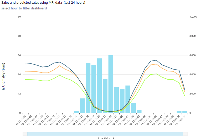
About the Authors:

 Tom Romano

Tom Romano is a Solutions Architect from Tampa, FL. Tom is a member the Service Creation team for the World Wide Public Sector, who assists GovTech and EdTech customers as they create new solutions that are cloud-native, event-driven, and serverless. He is an enthusiastic Python programmer for both application development and data analytics. In his free time, Tom flies remote control model airplanes and enjoys vacationing around Florida.

Robert Maefs

Robert Maefs is a lead technologist currently working with Wrap, Inc. developing innovative Virtual Reality training simulations for law enforcement and corrections. He is a repeat entrepreneur with expertise bringing mature technologies to under-served industries. In his personal life, Robert nerds out with board games and 3D printing.

Mark Curtis

Mark Curtis is a Senior Solutions Architect at AWS. At AWS he helps EdTech and GovTech customers architect and modernize their applications using cloud native serverless services. Prior to joining AWS, he spent 18 years developing scalable applications for both EdTech and Government customers.

Juan Peredo

Juan Peredo is a Cloud Application Architect at AWS Professional Services. He enjoys working with customers to design, migrate, and optimize cloud native applications. He is a problem solver at heart who likes using emerging technologies to solve interesting problems.

Amazon EMR Serverless cost estimator

Post Syndicated from Radhika Ravirala original https://aws.amazon.com/blogs/big-data/amazon-emr-serverless-cost-estimator/

Amazon EMR Serverless is a serverless option in Amazon EMR that makes it easy for data analysts and engineers to run applications using open-source big data analytics frameworks such as Apache Spark and Hive without configuring, managing, and scaling clusters or servers. You get all the features of the latest open-source frameworks with the performance-optimized runtime of Amazon EMR, and without having to plan and operate instances and clusters.

With Amazon EMR, you can run your analytics applications on dedicated EMR clusters, on existing Amazon Elastic Kubernetes Service (Amazon EKS) clusters, or using the new EMR Serverless deployment option where you don’t have to manage clusters or instances. When you build a Spark or Hive application using an Amazon EMR release, say Amazon EMR 6.8, you can run the application on EMR clusters, on EKS clusters using Amazon EMR on EKS, or using EMR Serverless without having to change the application.

To learn about the benefits of each deployment option in EMR Serverless, refer to What are some of the feature differences between EMR Serverless and Amazon EMR on EC2? in the Amazon EMR FAQ. You can also learn about the pricing for these options from the Amazon EMR pricing page. Many customers already run data analytics applications on EMR clusters, and find that the new serverless option is simpler and less expensive.

In this post, we discuss how you can estimate what it may cost to run an application that currently runs on EMR clusters using the new serverless option, and perform this analysis simply by using your current application metrics. This approach helps you evaluate and adopt the deployment option that is most cost effective for the application. However, the Amazon EMR pricing page doesn’t tell you how you can easily estimate the cost of running your existing EMR cluster applications on EMR Serverless. In the following sections, we describe an approach that enables you to do that.

Although the example in this post discusses how you can get a cost estimate for applications running on EMR clusters, you can also use the approach if you’re running a Spark or Hive application elsewhere, and want to estimate the cost of running it on EMR Serverless. For example, if you run self-managed Spark or Hive applications on Amazon Elastic Compute Cloud (Amazon EC2) clusters, or if you run Spark jobs on AWS Glue, we show you how you can use this approach to estimate the cost of running the application on EMR Serverless.

Estimating the cost of running applications on your EMR cluster

When you run applications on Amazon EMR clusters, you’re separately charged for the following:

  1. The Amazon EC2 price of running cluster instances (the price for the underlying servers)
  2. The price for Amazon Elastic Block Store (Amazon EBS) volumes, if you choose to attach EBS volumes
  3. The Amazon EMR price for the cluster instances

The total cost of running the cluster includes all three. There are a variety of Amazon EC2 pricing options you can choose from, including On Demand, 1-year and 3-year Reserved Instances, Capacity Savings Plans, and Spot Instances. The Amazon EC2 pricing option that you choose determines (a), the Amazon EC2 price. The cost of running the application on EMR clusters is the sum of (a), (b), and (c). You can compute this cost for the lifetime of running the cluster (from the time a cluster is started to the time the cluster is terminated), or for a specific period of time while the cluster is running. We recommend running the former, that is to compute (a), (b), and (c) from the time the cluster is started to the time the cluster is terminated. If you have set up tags for your Amazon EMR cluster, you can easily get the detailed cost report for your EMR cluster using AWS Cost Explorer.

Estimating the cost of running the same applications using EMR Serverless

When you run the same applications using EMR Serverless, you pay for the amount of vCPU, memory, and storage resources consumed by your applications. There is no separate charge for EC2 instances or EBS volumes. And, you only pay for the resources that are actually used by the application and not for EC2 instances provisioned. For example, when running applications on EMR clusters, when an EC2 instance in the cluster is partially utilized (say, 16 GB memory is used out of 64 GB available on the instance, or 4 VCPUs are utilized out of 16 VCPUs available on the instance), or when the EC2 instance is idle (for example, when the instance is initializing or waiting for an application to start), you still incur Amazon EC2, Amazon EMR, and Amazon EBS charges for the full EC2 instance and for the duration that the instance is active in the EMR cluster. With EMR Serverless, you only pay for the vCPU, memory, and storage resources used from the time workers start to run your Spark or Hive job until the time they stop.

To estimate the cost of running your EMR Spark or Hive application on EMR Serverless, you need to first aggregate the total compute vCore-seconds, memory MB-seconds, and storage GB-seconds consumed by each YARN application that ran on your EMR cluster, from the time the YARN container is started to the time the YARN container is terminated. You can obtain these metrics from YARN resource manager logs accessible from YARN timeline server or YARN CLI tools. You can retrieve the running time, vCore-seconds, and memory MB-seconds used by each of the YARN applications.

If your cluster only runs Spark applications, there is a simpler approach to estimate. Instead of obtaining the vCore-seconds, memory MB-seconds, and storage GB-seconds from YARN resource manager logs, you can obtain these metrics from Spark event logs. We have provided the tool EMR Servless Estimator, which can parse the Spark event logs for your applications and provide the aggregated metrics for your cost estimate.

After you get the usage metrics for your application, you can compute the estimated EMR Serverless cost using EMR Serverless pricing. Simply multiple your aggregated vCore-seconds with EMR Serverless vCPU pricing per second, multiply aggregated memory MB-seconds with the EMR Serverless memory pricing per second, and multiply storage GB-seconds with the EMR Serverless storage pricing per second (only if the storage requirements exceed 20 GB per worker). By adding up these costs for vCPU, memory, and storage, you can compare the cost of running the same applications on EMR Serverless.

In this approach, we assume that the performance of the application is equivalent. In other words, the size (vCPU, memory) and runtime duration for each YARN container on the EMR cluster is the same as the number, size, and runtime duration of workers needed to run the application on EMR Serverless. We make this assumption because the EMR runtime for an EMR release is the same regardless of whether the application is run on an EMR cluster or on EMR Serverless.

Example

Let’s do a sample cost comparison of Amazon EMR on EC2 and EMR Serverless using a single cluster.

We ran a Spark application on an EMR cluster with five nodes (one primary, two core, and two task and gathered YARN metrics using the YARN CLI. The following code shows our aggregate resource allocation.

aggregate resource allocation

We computed the Amazon EMR on EC2 costs as follows:

  • Cluster instances
    • Primary: m5.2xlarge:1
    • Core: r5.2xlarge:2
    • Task: r5.2xlarge:2
  • Cluster runtime = 18 min
  • Instance on-demand cost
    • m5.2xlarge (8 vCPU, 32 GiB memory)
      • Amazon EC2: $0.384/hr
      • Amazon EMR incremental: $0.096/hr
    • r5.2xlarge (8 vCPU, 64 GiB memory)
      • Amazon EC2: $0.504/hr
      • Amazon EMR incremental: $0.126/hr

The following is the EMR on EC2 cost calculation:

  • Amazon EMR cost = ((1 primary node x $0.096/hr) + (2 core nodes x $ 0.126/hr) + (2 task nodes x $0.126/hr)) = $0.60
  • Amazon EC2 cost = ((1 primary x $0.384 /hr ) + (2 core nodes x $0.504/hr) + (2 task nodes x $0.504/hr)) = $2.40
  • Amazon EMR on EC2 cluster cost/hr = $0.6 + $2.40 = $3/hr * 8/60 hr (runtime in hrs)

The total Amazon EMR on Amazon EC2 cost is $0.40/hr.

To calculate EMR Serverless cost, aggregate the vCore-seconds and memory MB-seconds for the same application you ran previously on the EMR cluster. Then multiply those numbers with the EMR Serverless vCPU and memory price. Our calculation results are as follows:

  • Total_vcore_seconds = 5737
  • Total_Memory_mb_seconds = 120156631
  • Convert to vCPU/hr and memory-GB/hr:
    • Aggregated vCPU/hr: 5737/(60*60)=1.59
    • Aggregated memory/hr: 120156631/(60*60*1024)=32.5
  • Total vCPU-hours cost = 33 vCPU * 0.052624 VCPU/hr * 8/60 = $0.23
  • Total memory GB cost = 1.59 MB * 0.0057785 memory/hr * 8/60 = $0.00122

In this example, the total EMR Serverless cost is $0.231, a 42% reduction.

Conclusion

Amazon EMR Serverless is a recently launched serverless option in Amazon EMR that makes it easy to run open-source frameworks such as Spark and Hive without configuring, managing, and scaling clusters. Customers that already use EMR clusters want to understand how they can estimate the cost of running their EMR applications using EMR Serverless. We have presented an approach that you can use to conduct a cost analysis based on analyzing application metrics from your EMR clusters.

We hope you give this a try, and share your feedback with us!


About the authors

Radhika Ravirala is the Principal Product Manager at AWS.

Matthew Liem is the Senior Solution Architecture Manager at AWS.

Analyze real-time streaming data in Amazon MSK with Amazon Athena

Post Syndicated from Scott Rigney original https://aws.amazon.com/blogs/big-data/analyze-real-time-streaming-data-in-amazon-msk-with-amazon-athena/

Recent advances in ease of use and scalability have made streaming data easier to generate and use for real-time decision-making. Coupled with market forces that have forced businesses to react more quickly to industry changes, more and more organizations today are turning to streaming data to fuel innovation and agility.

Amazon Managed Streaming for Apache Kafka (MSK) is a fully managed service that makes it easy to build and run applications that use Apache Kafka, an open-source distributed event streaming platform designed for high-performance data pipelines, streaming analytics, data integration, and mission-critical applications. With Amazon MSK, you can capture real-time data from a wide range of sources such as database change events or web application user clickstreams. Since Kafka is highly optimized for writing and reading fresh data, it’s a great fit for operational reporting. However, gaining insight from this data often requires a specialized stream processing layer to write streaming records to a storage medium like Amazon S3, where it can be accessed by analysts, data scientists, and data engineers for historical analysis and visualization using tools like Amazon QuickSight.

When you want to analyze data where it lives and without developing separate pipelines and jobs, a popular choice is Amazon Athena. With Athena, you can use your existing SQL knowledge to extract insights from a wide range of data sources without learning a new language, developing scripts to extract (and duplicate) data, or managing infrastructure. Athena supports over 25 connectors to popular data sources including Amazon DynamoDB and Amazon Redshift which give data analysts, data engineers, and data scientists the flexibility to run SQL queries on data stored in databases running on-premises or in the cloud alongside data stored in Amazon S3. With Athena, there’s no data movement and you pay only for the queries you run.

What’s new

Starting today, you can now use Athena to query streaming data in MSK and self-managed Apache Kafka. This enables you to run analytical queries on real-time data held in Kafka topics and join that data with other Kafka topics as well as other data in your Amazon S3 data lake – all without the need for separate processes to first store the data on Amazon S3.

Solution overview

In this post, we show you how to get started with real-time SQL analytics using Athena and its connector for MSK. The process involves:

  1. Registering the schema of your streaming data with AWS Glue Schema Registry. Schema Registry is a feature of AWS Glue that allows you to validate and reliably evolve streaming data against JSON schemas. It can also serialize data into a compressed format, which helps you save on data transfer and storage costs.
  2. Creating a new instance of the Amazon Athena MSK Connector. Athena connectors are pre-built applications that run as serverless AWS Lambda applications, so there’s no need for standalone data export processes.
  3. Using the Athena console to run interactive SQL queries on your Kafka topics.

Get started with Athena’s connector for Amazon MSK

In this section, we’ll cover the steps necessary to set up your MSK cluster to work with Athena to run SQL queries on your Kafka topics.

Prerequisites

This post assumes you have a serverless or provisioned MSK cluster set up to receive streaming messages from a producing application. For information, see Setting up Amazon MSK and Getting started using Amazon MSK in the Amazon Managed Streaming for Apache Kafka Developer Guide.

You’ll also need to set up a VPC and a security group before you use the Athena connector for MSK. For more information, see Creating a VPC for a data source connector. Note that with MSK Serverless, VPCs and security groups are created automatically, so you can get started quickly.

Define the schema of your Kafka topics with AWS Glue Schema Registry

To run SQL queries on your Kafka topics, you’ll first need to define the schema of your topics as Athena uses this metadata for query planning. AWS Glue makes it easy to do this with its Schema Registry feature for streaming data sources.

Schema Registry allows you to centrally discover, control, and evolve streaming data schemas for use in analytics applications such as Athena. With AWS Glue Schema Registry, you can manage and enforce schemas on your data streaming applications using convenient integrations with Apache Kafka. To learn more, see AWS Glue Schema Registry and Getting started with Schema Registry.

If configured to do so, the producer of data can auto-register its schema and changes to it with AWS Glue. This is especially useful in use cases where the contents of the data is likely to change over time. However, you can also specify the schema manually and will resemble the following JSON structure.

{
  "tableName": "orders",
  "schemaName": "customer_schema",
  "topicName": "orders",
  "message": {
    "dataFormat": "json",
    "fields": [
      {
        "name": "customer_id",
        "mapping": "customer_id",
        "type": "VARCHAR"
      },
      {
        "name": "item_id",
        "mapping": "item_id",
        "type": "INTEGER"
      }
    ]
  }
}

When setting up your Schema Registry, be sure to give it an easy-to-remember name, such as customer_schema, because you’ll reference it within SQL queries as you’ll see later on. For additional information on schema set up, see Schema examples for the AWS Glue Schema Registry.

Configure the Athena connector for MSK

With your schema registered with Glue, the next step is to set up the Athena connector for MSK. We recommend using the Athena console for this step. For more background on the steps involved, see Deploying a connector and connecting to a data source.

In Athena, federated data source connectors are applications that run on AWS Lambda and handle communication between your target data source and Athena. When a query runs on a federated source, Athena calls the Lambda function and tasks it with running the parts of your query that are specific to that source. To learn more about the query execution workflow, see Using Amazon Athena Federated Query in the Amazon Athena User Guide.

Start by accessing the Athena console and selecting Data sources on the left navigation, then choose Create data source:

Next, search for and select Amazon MSK from the available connectors and select Next.

In Data source details, give your connector a name, like msk, that’s easy to remember and reference in your future SQL queries. Under Connection details section, select Create Lambda function. This will bring you to the AWS Lambda console where you’ll provide additional configuration properties.

In the Lambda application configuration screen (not shown), you’ll provide the Application settings for your connector. To do this, you’ll need a few properties from your MSK cluster and schema registered in Glue.

On another browser tab, use the MSK console to navigate to your MSK cluster and then select the Properties tab. Here you’ll see the VPC subnets and security group IDs from your MSK cluster which you’ll provide in the SubnetIds and SecurityGroupIds fields in the Athena connector’s Application settings form. You can find the value for KafkaEndpoint by clicking View client information.

In the AWS Glue console, navigate to your Schema Registry to find the GlueRegistryArn for the schema you wish to use with this connector.

After providing these and the other required values, click Deploy.

Return to the Athena console and enter the name of the Lambda function you just created in the Connection details box, then click Create data source.

Run queries on streaming data using Athena

With your MSK data connector set up, you can now run SQL queries on the data. Let’s explore a few use cases in more detail.

Use case: interactive analysis

If you want to run queries that aggregate, group, or filter your MSK data, you can run interactive queries using Athena. These queries will run against the current state of your Kafka topics at the time the query was submitted.

Before running any queries, it may be helpful to validate the schema and data types available within your Kafka topics. To do this, run the DESCRIBE command on your Kafka topic, which appears in Athena as a table, as shown below. In this query, the orders table corresponds to the topic you specified in the Schema Registry.

DESCRIBE msk.customer_schema.orders

Now that you know the contents of your topic, you can begin to develop analytical queries. A sample query for a hypothetical Kafka topic containing e-commerce order data is shown below:

SELECT customer_id, SUM(order_total)
FROM msk.customer_schema.orders
GROUP BY customer_id

Because the orders table (and underlying Kafka topic) can contain an unbounded stream of data, the query above is likely to return a different value for SUM(order_total) with each execution of the query.

If you have data in one topic that you need to join with another topic, you can do that too:

SELECT t1.order_id, t2.item_id
FROM msk.customer_schema.orders as t1
JOIN msk.customer_schema.items as t2
ON t1.id = t2.id

Use case: ingesting streaming data to a table on Amazon S3

Federated queries run against the underlying data source which ensures interactive queries, like the ones above, are evaluated against the current state of your data. One consideration is that repeatedly running federated queries can put additional load on the underlying source. If you plan to perform multiple queries on the same source data, you can use Athena’s CREATE TABLE AS SELECT, also known as CTAS, to store the results of a SELECT query in a table on Amazon S3. You can then run queries on your newly created table without going back to the underlying source each time.

CREATE TABLE my_kafka_data
WITH (format = 'Parquet', 
      write_compression = 'SNAPPY')
AS
SELECT order_id, item_id, timestamp
FROM msk.customer_schema.orders

If you plan to do additional downstream analysis on this data, for example within dashboards on Amazon QuickSight, you can enhance the solution above by periodically adding new data to your table. To learn more, see Using CTAS and INSERT INTO for ETL and data analysis. Another benefit of this approach is that you can secure these tables with row-, column-, and table-level data governance policies powered by AWS Lake Formation to ensure only authorized users can access your table.

What else can you do?

With Athena, you can use your existing SQL knowledge to run federated queries that generate insights from a wide range of data sources without learning a new language, developing scripts to extract (and duplicate) data, or managing infrastructure. Athena provides additional integrations with other AWS services and popular analytics tools and SQL IDEs that allow you to do much more with your data. For example, you can:

  • Visualize the data in business intelligence applications like Amazon QuickSight
  • Design event-driven data processing workflows with Athena’s integration with AWS Step Functions
  • Unify multiple data sources to produce rich input features for machine learning in Amazon SageMaker

Conclusion

In this post, we learned about the newly released Athena connector for Amazon MSK. With it, you can run interactive queries on data held in Kafka topics running in MSK or self-managed Apache Kafka. This helps you bring real-time insights to dashboards or enable point-in-time analysis of streaming data to answer time-sensitive business questions. We also covered how to periodically ingest new streaming data into Amazon S3 without the need for a separate sink process. This simplifies recurring analysis of your data without incurring round-trip queries to your underlying Kafka clusters and makes it possible to secure the data with access rules powered by Lake Formation.

We encourage you to evaluate Athena and federated queries on your next analytics project. For help getting started, we recommend the following resources:


About the authors

Scott Rigney is a Senior Technical Product Manager with Amazon Web Services (AWS) and works with the Amazon Athena team based out of Arlington, Virginia. He is passionate about building analytics products that enable enterprises to make data-driven decisions.

Kiran Matty is a Principal Product Manager with Amazon Web Services (AWS) and works with the Amazon Managed Streaming for Apache Kafka (Amazon MSK) team based out of Palo Alto, California. He is passionate about building performant streaming and analytical services that help enterprises realize their critical use cases.

Prepare for consolidated controls view and consolidated control findings in AWS Security Hub

Post Syndicated from Priyanka Prakash original https://aws.amazon.com/blogs/security/prepare-for-consolidated-controls-view-and-consolidated-control-findings-in-aws-security-hub/

Currently, AWS Security Hub identifies controls and generates control findings in the context of security standards. Security Hub is aiming to release two new features in the first quarter of 2023 that will decouple controls from standards and streamline how you view and receive control findings.

The new features to be released are consolidated controls view and consolidated control findings. Consolidated controls view will provide you with a comprehensive view within the Security Hub console of your controls across security standards. This feature will also introduce a single unique identifier for each control across security standards.

Consolidated control findings will streamline your control findings. When this feature is turned on, Security Hub will produce a single finding for a security check even when a check is shared across multiple standards. This will reduce finding noise and help you focus on misconfigured resources in your AWS environment.

In this blog post, I’ll summarize the upcoming features, the benefit they bring to your organization, and how you can take advantage of them upon release.

Feature 1: Consolidated controls view

Currently, controls are identified, viewed, and managed in the context of individual security standards. In the Security Hub console, you first have to navigate to a specific standard to see a list of controls for that standard. Within the AWS Foundational Security Best Practices (FSBP) standard, Security Hub identifies controls by the impacted AWS service and a unique number (for example, IAM.1). For other standards, Security Hub includes the standard as part of the control identifier (for example, CIS 1.1 or PCI.AutoScaling.1).

After the release of consolidated controls view, you will be able to see a consolidated list of your controls from a new Controls page in the Security Hub console. Security Hub will also assign controls a consistent security control ID across standards. Following the current naming convention of the AWS FSBP standard, control IDs will include the relevant service and a unique number.

For example, the control AWS Config should be enabled is currently identified as Config.1 in the AWS FSBP standard, CIS 2.5 in the Center for Internet Security (CIS) AWS Foundations Benchmark v1.2.0, CIS 3.5 in the CIS AWS Foundations Benchmark v1.4.0, and PCI.Config.1 in the Payment Card Industry Data Security Standard (PCI DSS). After this release, this control will have a single identifier called Config.1 across standards. The single Controls page and consistent identifier will help you rapidly discover misconfigurations with minimal context-switching.

You’ll be able to enable a control for one or more enabled standards that include the control. You’ll also be able to disable a control for one or more enabled standards. As before, you can enable the standards that apply to your business case.

Changes to control finding fields and values after the release of consolidated controls view

After the release of consolidated controls view, note the following changes to control finding fields and values in the AWS Security Finding Format (ASFF).

ASFF field What changes after consolidated controls view release Example value before consolidated controls view release Example value after consolidated controls view release
Compliance.SecurityControlId A single control ID will apply across standards. ProductFields.ControlId will still provide the standards-based control ID. Not applicable (new field) EC2.2
Compliance.AssociatedStandards Will show the standards that a control is enabled for. Not applicable (new field) [{“StandardsId”: “aws-foundational-security-best-practices/v/1.0.0”}]
ProductFields.RecommendationUrl This field will no longer reference a standard. https://docs.aws.amazon.com/console/securityhub/PCI.EC2.2/remediation https://docs.aws.amazon.com/console/securityhub/EC2.2/remediation
Remediation.Recommendation.Text This field will no longer reference a standard. “For directions on how to fix this issue, please consult the AWS Security Hub PCI DSS documentation.” “For instructions on how to fix this issue, see the AWS Security Hub documentation for EC2.2.”
Remediation.Recommendation.Url This field will no longer reference a standard. https://docs.aws.amazon.com/console/securityhub/PCI.EC2.2/remediation https://docs.aws.amazon.com/console/securityhub/EC2.2/remediation

Feature 2: Consolidated control findings

Currently, multiple standards contain separate controls for the same security check. Security Hub generates a separate finding per standard for each related control that is evaluated by the same security check.

After release of the consolidated control findings feature, you’ll be able to unify control findings across standards and reduce finding noise. This, in turn, will help you more quickly investigate and remediate failed findings. When you turn on consolidated control findings, Security Hub will generate a single finding or finding update for each security check of a control, even if the check is shared across multiple standards.

For example, after you turn on the feature, you will receive a single finding for a security check of Config.1 even if you’ve enabled this control for the AWS FSBP standard, CIS AWS Foundations Benchmark v1.2.0, CIS AWS Foundations Benchmark v1.4.0, and PCI DSS. If you don’t turn on consolidated control findings, you will receive four separate findings for a security check of Config.1 if you’ve enabled this control for the AWS FSBP standard, CIS AWS Foundations Benchmark v1.2.0, CIS AWS Foundations Benchmark v1.4.0, and PCI DSS.

Changes to control finding fields and values after turning on consolidated control findings

If you turn on consolidated control findings, note the following changes to control finding fields and values in the ASFF. These changes are in addition to the changes previously described for consolidated controls view.

ASFF field What changes after consolidated controls view release Example value before consolidated controls view release Example value after consolidated controls view release
GeneratorId This field will no longer reference a standard. aws-foundational-security-best-practices/v/1.0.0/Config.1 security-control/Config.1
Title This field will no longer reference a standard. PCI.Config.1 AWS Config should be enabled {
Id This field will no longer reference a standard. arn:aws:securityhub:eu-central-1:123456789012:subscription/pci-dss/v/3.2.1/PCI.IAM.5/finding/ab6d6a26-a156-48f0-9403-115983e5a956 arn:aws:securityhub:eu-central-1:123456789012:security-control/iam.9/finding/ab6d6a26-a156-48f0-9403-115983e5a956
ProductFields.ControlId This field will be removed in favor of a single, standard-agnostic control ID. PCI.EC2.2 Removed. See Compliance.SecurityControlId instead.
ProductFields.RuleId This field will be removed in favor of a single, standard-agnostic control ID. 1.3 Removed. See Compliance.SecurityControlId instead.
Description This field will no longer reference a standard. This PCI DSS control checks whether AWS Config is enabled in the current account and region. This AWS control checks whether AWS Config is enabled in the current account and region.
Severity Security Hub will no longer use the Product field to describe the severity of a finding. “Severity”: {
“Product”: 90,
“Label”: “CRITICAL”,
“Normalized”: 90,
“Original”: “CRITICAL”
},
“Severity”: {
“Label”: “CRITICAL”,
“Normalized”: 90,
“Original”: “CRITICAL”
},
Types This field will no longer reference a standard. [“Software and Configuration Checks/Industry and Regulatory Standards/PCI-DSS”] [“Software and Configuration Checks/Industry and Regulatory Standards”]
Compliance.RelatedRequirements This field will show related requirements across associated standards. [ “PCI DSS 10.5.2”,
“PCI DSS 11.5”]
[ “PCI DSS v3.2.1/10.5.2”,
“PCI DSS v3.2.1/11.5”,
“CIS AWS Foundations Benchmark v1.2.0/2.5”]
CreatedAt Format will remain the same, but value will reset when you turn on consolidated control findings. 2022-05-05T08:18:13.138Z 2022-09-25T08:18:13.138Z
FirstObservedAt Format will remain the same, but value will reset when you turn on consolidated control findings. 2022-05-07T08:18:13.138Z 2022-09-28T08:18:13.138Z
ProductFields.RecommendationUrl This field will be replaced by Remediation.Recommendation.Url. https://docs.aws.amazon.com/console/securityhub/EC2.2/remediation Removed. See Remediation.Recommendation.Url instead.
ProductFields.StandardsArn This field will be replaced by Compliance.AssociatedStandards. arn:aws:securityhub:::standards/aws-foundational-security-best-practices/v/1.0.0 Removed. See Compliance.AssociatedStandards instead.
ProductFields.StandardsControlArn This field will be removed because Security Hub will generate one finding for a security check across standards. arn:aws:securityhub:us-east-1:123456789012:control/aws-foundational-security-best-practices/v/1.0.0/Config.1 Removed.
ProductFields.StandardsGuideArn This field will be replaced by Compliance.AssociatedStandards. arn:aws:securityhub:::ruleset/cis-aws-foundations-benchmark/v/1.2.0 Removed. See Compliance.AssociatedStandards instead.
ProductFields.StandardsGuideSubscriptionArn This field will be removed because Security Hub will generate one finding for a security check across standards. arn:aws:securityhub:us-east-2:123456789012:subscription/cis-aws-foundations-benchmark/v/1.2.0 Removed.
ProductFields.StandardsSubscriptionArn This field will be removed because Security Hub will generate one finding for a security check across standards. arn:aws:securityhub:us-east-1:123456789012:subscription/aws-foundational-security-best-practices/v/1.0.0 Removed.
ProductFields.aws/securityhub/FindingId This field will no longer reference a standard. arn:aws:securityhub:us-east-1::product/aws/securityhub/arn:aws:securityhub:us-east-1:123456789012:subscription/aws-foundational-security-best-practices/v/1.0.0/Config.1/finding/751c2173-7372-4e12-8656-a5210dfb1d67 arn:aws:securityhub:us-east-1::product/aws/securityhub/arn:aws:securityhub:us-east-1:123456789012:security-control/Config.1/finding/751c2173-7372-4e12-8656-a5210dfb1d67

New values for customer-provided finding fields after turning on consolidated control findings

When you turn on consolidated control findings, Security Hub will archive the existing findings and generate new findings. To view archived findings, you can visit the Findings page of the Security Hub console with the Record state filter set to ARCHIVED, or use the GetFindings API action. Updates you’ve made to the original finding fields in the Security Hub console or by using the BatchUpdateFindings API action will not be preserved in the new findings (if needed, you can recover this data by referring to the archived findings).

Note the following changes to customer-provided control finding fields when you turn on consolidated control findings.

Customer-provided ASFF field Description of change after turning on consolidated control findings
Confidence Will reset to empty state.
Criticality Will reset to empty state.
Note Will reset to empty state.
RelatedFindings Will reset to empty state.
Severity The default severity of the finding (matches the severity of the control).
Types Will reset to standard-agnostic value.
UserDefinedFields Will reset to empty state.
VerificationState Will reset to empty state.
Workflow New failed findings will have a default value of NEW. New passed findings will have a default value of RESOLVED.

How to turn consolidated control findings on and off

Follow these instructions to turn consolidated control findings on and off.

New accounts

If you enable Security Hub for an AWS account for the first time on or after the time when consolidated control findings is released, by default consolidated control findings will be turned on for your account. You can turn it off at any time. However, we recommend keeping it turned on to minimize finding noise.

If you use the Security Hub integration with AWS Organizations, consolidated control findings will be turned on for new member accounts if the administrator account has turned on the feature. If the administrator account has turned it off, it will be turned off for new subordinate AWS accounts (member accounts) as well.

Existing accounts

If your Security Hub account already existed before consolidated control findings is released, your account will have consolidated control findings turned off by default. You can turn it on at any time. We recommend turning it on to minimize finding noise. If you use AWS Organizations, consolidated control findings will be turned on or off for existing member accounts based on the settings of the administrator account.

To turn consolidated control findings on and off (Security Hub console)

  1. In the navigation pane, choose Settings.
  2. Choose the General tab.
  3. For Controls, turn on Consolidated control findings. Turn it off to receive multiple findings for each standard.
  4. Choose Save.

To turn consolidated control findings on and off (Security Hub API)

  • Run the UpdateSecurityHubConfiguration API action. Use the new ControlFindingGenerator attribute to change whether an account uses consolidated control findings:
    • To turn on consolidated control findings, set ControlFindingGenerator equal to SECURITY_CONTROL.
    • To turn it off, set ControlFindingGenerator equal to STANDARD_CONTROL.

To turn consolidated control findings on and off (AWS CLI)

  • In the AWS CLI, run the update-security-hub-configuration command. Use the new control-finding-generator attribute to change whether an account uses consolidated control findings:
    • To turn on consolidated control findings, set control-finding-generator equal to SECURITY_CONTROL.
    • To turn it off, set control-finding-generator equal to STANDARD_CONTROL.

API permissions for consolidated control findings

You’ll need AWS Identity and Access Management (IAM) permissions for the following new API operations in order for consolidated control findings to work as expected:

  • BatchGetSecurityControls – Returns account and Region-specific data about a batch of controls.
  • ListSecurityControlDefinitions – Returns information about controls that apply to a specified standard.
  • ListStandardsControlAssociations – Identifies whether a control is currently associated with or dissociated from each enabled standard.
  • BatchGetStandardsControlAssociations – For a batch of controls, identifies whether each control is currently associated with or dissociated from a specified standard.
  • BatchUpdateStandardsControlAssociations – Used to associate a control with enabled standards that include the control, or to dissociate a control from enabled standards. This is a batch substitute for the UpdateStandardsControl API action if an administrator doesn’t want to allow member accounts to associate or dissociate controls.
  • BatchGetControlEvaluations (private API) – Retrieves the enablement and compliance status of a control, the findings count for a control, and the overall security score for controls.

How to prepare for control finding field and value changes

If your workflows don’t rely on the specific format of any control finding fields, no action is required to prepare for the feature releases. We recommend that you immediately turn on consolidated control findings.

Consider waiting to turn on consolidated control findings if you currently rely on the Automated Security Response on AWS solution for predefined response and remediation actions. That solution does not yet support consolidated control findings. If you turn consolidated control findings on now, actions you deployed using the Automated Security Response solution will no longer work.

If you rely on the specific format of any control finding fields (for example, for custom automation), carefully review the upcoming finding field and value changes to ensure that your workflows will continue to function as intended. Note that the changes noted in the first table in this post might impact you if you rely on the specified control finding fields and values.

The changes noted in the second table and third table in this post will only impact you if you turn on consolidated control findings. For example, if you rely on ProductFields.ControlId, GeneratorId, or Title, you’ll be impacted if you turn on consolidated control findings. As another example, if you’ve created an Amazon CloudWatch Events rule that initiates an action for a specific control ID (such as invoking an AWS Lambda function if the control ID equals CIS 2.7), you’ll need to update the rule to use CloudTrail.2, the new Compliance.SecurityControlId field for that control.

If you’ve created custom insights by using the control finding fields or values that will change (see previous tables), we recommend updating those insights to use the new fields or values.

Conclusion

This post covered the control finding fields and values that will change in Security Hub after release of the consolidated controls view and consolidated control findings features. We recommend that you carefully review the changes and update your workflows to start using the new fields and values as soon as the features become available.

For more information about the upcoming changes, see the Security Hub user guide, which includes value changes for GeneratorId , control title changes, and sample control findings before and after the upcoming feature releases.

If you have feedback about this post, submit comments in the Comments section below. If you have questions about this post, start a new thread on the Security, Identity, & Compliance re:Post or contact AWS Support.

Want more AWS Security news? Follow us on Twitter.

Author

Priyanka Prakash

Priyanka is a technical writer for AWS Security Hub. She enjoys helping customers understand how to effectively monitor their environment and address security issues. Prior to joining AWS, Priyanka worked for a cloud monitoring startup. In her personal time, Priyanka enjoys cooking and hiking.

Create, Train and Deploy Multi Layer Perceptron (MLP) models using Amazon Redshift ML

Post Syndicated from Anuradha Karlekar original https://aws.amazon.com/blogs/big-data/create-train-and-deploy-multi-layer-perceptron-mlp-models-using-amazon-redshift-ml/

Amazon Redshift is a fully managed and petabyte-scale cloud data warehouse which is being used by tens of thousands of customers to process exabytes of data every day to power their analytics workloads. Amazon Redshift comes with a feature called Amazon Redshift ML which puts the power of machine learning in the hands of every data warehouse user, without requiring the users to learn any new programming language, ML concepts or ML tools. Redshift ML abstracts all the intricacies that are involved in the traditional ML approach around data warehouse which traditionally involved repetitive, manual steps to move data back and forth between the data warehouse and ML tools for running long, complex, iterative ML workflow.

Redshift ML uses Amazon SageMaker Autopilot and Amazon SageMaker Neo in the background to make it easy for SQL users such as data analysts, data scientists, BI experts and database developers to create, train, and deploy machine learning (ML) models using familiar SQL commands and then use these models to make predictions on new data for use cases such as customer churn prediction, basket analysis for sales prediction, manufacturing unit lifetime value prediction, and product recommendations. Redshift ML makes the model available as SQL function within the Amazon Redshift data warehouse so you can easily use it in queries and reports.

Amazon Redshift ML supports supervised learning, including regression, binary classification, multi-class classification, and unsupervised learning using K-Means. You can optionally specify XGBoost, MLP, and linear learner model types, which are supervised learning algorithms used for solving either classification or regression problems, and provide a significant increase in speed over traditional hyperparameter optimization techniques. Amazon Redshift ML also supports bring-your-own-model to either import existing SageMaker models that are built using algorithms supported by SageMaker Autopilot, which can be used for local inference; or for the unsupported algorithms, one can alternatively invoke remote SageMaker endpoints for remote inference.

In this blog post, we show you how to use Redshift ML to solve binary classification problem using the Multi Layer Perceptron (MLP) algorithm, which explores different training objectives and chooses the best solution from the validation set.

A multilayer perceptron (MLP) is a deep learning method which deals with training multi-layer artificial neural networks, also called Deep Neural Networks. It is a feedforward artificial neural network that generates a set of outputs from a set of inputs. An MLP is characterized by several layers of input nodes connected as a directed graph between the input and output layers. MLP uses backpropagation for training the network. MLP is widely used for solving problems that require supervised learning as well as research into computational neuroscience and parallel distributed processing. It is also used for speech recognition, image recognition and machine translation.

As far as MLP usage with Redshift ML (powered by Amazon SageMaker Autopilot) is concerned, it supports tabular data as of now.

Solution Overview

To use the MLP algorithm, you need to provide inputs or columns representing dimensional values and also the label or target, which is the value you’re trying to predict.

With Redshift ML, you can use MLP on tabular data for regression, binary classification or multiclass classification problems. What is more unique about MLP is, is that the output function of MLP can be a linear or a continuous function as well. It need not be a straight line like the general regression model provides.

In this solution, we use binary classification to detect frauds based upon the credit cards transaction data. The difference between classification models and MLP is that logistic regression uses a logistic function, while perceptrons use a step function. Using the multilayer perceptron model, machines can learn weight coefficients that help them classify inputs. This linear binary classifier is highly effective in arranging and categorizing input data into different classes, allowing probability-based predictions and classifying items into multiple categories. Multilayer Perceptrons have the advantage of learning non-linear models and the ability to train models in real-time.

For this solution, we first ingest the data into Amazon Redshift, we then distribute it for model training and validation, then use Amazon Redshift ML specific queries for model creation and thereby create and utilize the generated SQL function for being able to finally predict the fraudulent transactions.

Prerequisites

To get started, we need an Amazon Redshift cluster or an Amazon Redshift Serverless endpoint and an AWS Identity and Access Management (IAM) role attached that provides access to SageMaker and permissions to an Amazon Simple Storage Service (Amazon S3) bucket.

For an introduction to Redshift ML and instructions on setting it up, see Create, train, and deploy machine learning models in Amazon Redshift using SQL with Amazon Redshift ML.

To create a simple cluster with a default IAM role, see Use the default IAM role in Amazon Redshift to simplify accessing other AWS services.

Data Set Used

In this post, we use the Credit Card Fraud detection data to create, train and deploy MLP model which can be used further to identify fraudulent transactions from the newly captured transaction records.

The dataset contains transactions made by credit cards in September 2013 by European cardholders.
This dataset presents transactions that occurred in two days, where we have 492 frauds out of 284,807 transactions. The dataset is highly unbalanced, the positive class (frauds) account for 0.172% of all transactions.

It contains only numerical input variables which are the result of a Principal Component Analysis transformation. Due to confidentiality issues, the original features and more background information about the data is not provided. Features V1, V2, … V28 are the principal components obtained with PCA, the only features which have not been transformed with PCA are ‘Time’ and ‘Amount’. Feature ‘Time’ contains the seconds elapsed between each transaction and the first transaction in the dataset. The feature ‘Amount’ is the transaction Amount. Feature ‘Class’ is the response variable and it takes value 1 in case of fraud and 0 otherwise.

Here are sample records:

Prepare the data

Load the credit card dataset into Amazon Redshift using the following SQL. You can use the Amazon Redshift query editor v2 or your preferred SQL tool to run these commands.

Alternately we have provided a notebook you may use to execute all the sql commands that can be downloaded here. You will find instructions in this blog on how to import and use notebooks.

To create the table, use the following command:

CREATE TABLE creditcardsfrauds (
    txtime integer,
    v1 float8,
    v2 float8,
    v3 float8,
    v4 float8,
    v5 float8,
    v6 float8,
    v7 float8,
    v8 float8,
    v9 float8,
    v10 float8,
    v11 float8,
    v12 float8,
    v13 float8,
    v14 float8,
    v15 float8,
    v16 float8,
    v17 float8,
    v18 float8,
    v19 float8,
    v20 float8,
    v21 float8,
    v22 float8,
    v23 float8,
    v24 float8,
    v25 float8,
    v26 float8,
    v27 float8,
    v28 float8,
    amount float8,
    class integer
);

Load the data

To load data into Amazon Redshift, use the following COPY command:

COPY creditcardsfrauds
FROM 's3://redshift-ml-blog-mlp/creditcard.csv' 
IAM_ROLE default
CSV QUOTE as '\"' delimiter ',' IGNOREHEADER 1 maxerror 100
REGION 'us-east-1';

Before creating the model, we want to divide our data into two sets by splitting 80% of the dataset for training and 20% for validation, which is a common practice in ML. The training data is input to the ML model to identify the best possible algorithm for the model. After the model is created, we use the validation data to validate the model accuracy.

So, in ‘creditcardsfrauds’ table, we check the distribution of data based upon ‘txtime’ value and identify the cutoff for around 80% of the data to train the model.

With this, the highest txtime value comes to 120954 (based upon the distribution of txtime’s min, max, ranking by window function and ceil(count(*)*0.80) values)), based upon which we consider the transaction records having ‘txtime’ field value less than 120954 for creating training data. We then validate the accuracy of that model by seeing if it correctly identifies the fraudulent transactions by predicting its ‘class’ attribute on the remaining 20% of the data.

This distribution for 80% cutoff need not always be based upon ordered time. It can be picked up randomly as well, based upon the use case under consideration.

Create a model in Redshift ML

To create the model, use the following command:

 CREATE model creditcardsfrauds_mlp
FROM (select * from creditcardsfrauds where txtime < 120954)
TARGET class 
FUNCTION creditcardsfrauds_mlp_fn
IAM_ROLE default
MODEL_TYPE MLP
SETTINGS (
      S3_BUCKET '<<your-amazon-s3-bucket-name>>’,
      MAX_RUNTIME 9600
);

Here, in the settings section of the command, you need to set up an S3_BUCKET which is used to export the data that is sent to SageMaker and store model artifacts.

S3_BUCKET setting is a required parameter of the command, whereas MAX_RUNTIME is an optional one which specifies the maximum amount of time to train. The default value of this parameter is 90 minutes (5400 seconds), however you can override it by explicitly specifying it in the command, just like we have done it here by setting it to run for 9600 seconds.

The preceding statement initiates an Amazon SageMaker Autopilot process in the background to automatically build, train, and tune the best ML model for the input data. It then uses Amazon SageMaker Neo to deploy that model locally in the Amazon Redshift cluster or Amazon Redshift Serverless as a user-defined function (UDF).

You can use the SHOW MODEL command in Amazon Redshift to track the progress of your model creation, which should be in the READY state within the max_runtime parameter you defined while creating the model.

To check the status of the model, use the following command:

show model creditcardsfrauds_mlp;

We notice from the preceding table that the F1-score for the training data is 0.908, which shows very good performance accuracy.

To elaborate, F1-score is the harmonic mean of precision and recall. It combines precision and recall into a single number using the following formula:

Where, Precision means: Of all positive predictions, how many are really positive?

And Recall means: Of all real positive cases, how many are predicted positive?

F1 scores can range from 0 to 1, with 1 representing a model that perfectly classifies each observation into the correct class and 0 representing a model that is unable to classify any observation into the correct class. So higher F1 scores are better.

The following is the detailed tabular outcome for the preceding command after model training was done.

Model Name creditcardsfrauds_mlp
Schema Name public
Owner redshiftml
Creation Time Sun, 25.09.2022 16:07:18
Model State READY
validation:binary_f_beta 0.908864
Estimated Cost 112.296925
TRAINING DATA: .
Query SELECT * FROM CREDITCARDSFRAUDS WHERE TXTIME < 120954
Target Column CLASS
PARAMETERS: .
Model Type mlp
Problem Type BinaryClassification
Objective F1
AutoML Job Name redshiftml-20221118035728881011
Function Name creditcardsfrauds_mlp_fn
. creditcardsfrauds_mlp_fn_prob
Function Parameters txtime v1 v2 v3 v4 v5 v6 v7 v8 v9 v10 v11 v12 v13 v14 v15 v16 v17 v18 v19 v20 v21 v22 v23 v24 v25 v26 v27 v28 amount
Function Parameter Types int4 float8 float8 float8 float8 float8 float8 float8 float8 float8 float8 float8 float8 float8 float8 float8 float8 float8 float8 float8 float8 float8 float8 float8 float8 float8 float8 float8 float8 float8
IAM Role default
S3 Bucket redshift-ml-blog-mlp
Max Runtime 54000

Redshift ML now supports Prediction Probabilities for binary classification models. For classification problem in machine learning, for a given record, each label can be associated with a probability that indicates how likely this record really belongs to the label. With option to have probabilities along with the label, customers could use the classification results when confidence based on chosen label is higher than a certain threshold value returned by the model

Prediction probabilities are calculated by default for binary classification models and an additional function is created while creating model without impacting performance of the ML model.

In above snippet, you will notice that predication probabilities enhancements have added another function as a suffix (_prob) to model function with a name ‘creditcardsfrauds_mlp_fn_prob’ which could be used to get prediction probabilities.

Additionally, you can check the model explainability to understand which inputs contributed effectively to derive the prediction.

Model explainability helps to understand the cause of prediction by answering questions such as:

  • Why did the model predict a negative outcome such as blocking of credit card when someone travels to a different country and withdraws a lot of money in different currency?
  • How does the model make predictions? Lots of data for credit cards can be put in a tabular format and as per MLP process where a fully connected neural network of several layers is involved, we can tell which input feature actually contributed to the model output and its magnitude.
  • Why did the model make an incorrect prediction? E.g. Why is the card blocked even though the transaction is legitimate?
  • Which features have the largest influence on the behavior of the model? Is it just based upon the location where the credit card is swiped, or even the time of the day and unusual credit consumption that is influencing the prediction?

Run the following SQL command to retrieve the values from the explainability report:

SELECT json_table.report.explanations.kernel_shap.label0.global_shap_values 
FROM (select explain_model('creditcardsfrauds_mlp') as report) as json_table;

In the preceding screenshot, we have only selected the column that projects shapley values from the response returned by the explain_model function. If you notice the response of the query, the values in every json object show the contribution of different features in terms of influencing the prediction. E.g. from the preceding snippet, v14 feature is influencing the prediction the most and txtime feature does not really play any significant role in predicting ‘class’.

Model validation

Now let’s run the prediction query and validate the accuracy of the model on the validation dataset:

FROM (
  SELECT 
      CASE WHEN class =  
      creditcardsfrauds_mlp_fn(txtime,v1,v2,v3,v4,v5,v6,v7,v8,v9,v10,v11,v12,v13,v14,v15,v16,v17,v18,v19,v20,v21,v22,v23,v24,v25,v26,v27,v28,amount) 
      THEN 'PredictedMatchesActual' 
      else 'NoMatch' 
      END as actualvspredicted
    FROM creditcardsfrauds 
    WHERE txtime >= 120954
) 
group by actualvspredicted

We can observe here that Redshift ML is able to identify 99.88 percent of the transactions correctly as fraudulent or non-fraudulent.

Now you can continue to use this SQL function creditcardsfrauds_mlp_fn for local inference in any part of the SQL query while analyzing, visualizing or reporting the newly arriving as well as existing data!

--CREATE A STAGING TABLE TO HOLD NEWLY ARRIVING DATA FROM THE SOURCE WHICH WILL NOT CONAIN THE CLASS COLUMN - AS IT IS TO BE PREDICTED
DROP TABLE creditcardsfrauds_staging;
CREATE TABLE creditcardsfrauds_staging as (select * from creditcardsfrauds limit 0);
Alter table creditcardsfrauds_staging drop column class;

--LETS CONSIDER ONLY ONE RECORD HERE WHICH HAS NEWLY ARRIVED
insert into creditcardsfrauds_staging values(174965,-39999.11383160738512,0.58586417180689,-5.39973021073242,1.81709247345531,-0.840618465991056,-2.94354779071974,-2.20800192003372,1.05873267723056,-1.63233334974982,-5000.24598383776964,11.93351953683592,-53046479695456,-1.12745457501155,-666666.41662797597451,0.141237234328704,-2.54949823633632,-4.61471706851594,-10.47813794126038,-0.0354803664667244,0.306270740368093,0.583275998701341,-0.269208637986581,-0.456107772584008,-0.183659129549716,-0.328167759255761,0.606115810329683,0.884875539542905,-0.253700318894381,-2450000000);

--USE THE FUNCTION TO PREDICT THE VALUE OF CLASS
SELECT txtime, creditcardsfrauds_mlp_fn(txtime,v1,v2,v3,v4,v5,v6,v7,v8,v9,v10,v11,v12,v13,v14,v15,v16,v17,v18,v19,v20,v21,v22,v23,v24,v25,v26,v27,v28,amount)
FROM creditcardsfrauds_staging;

Here the output 1 means that the newly captured transaction is fraudulent as per the inference.

Additionally, you can change the above query to include prediction probabilities of label output for the above scenario and decide if you still like to use the prediction by the model.

--USE THE FUNCTION TO PREDICT THE VALUE OF CLASS ALONG WITH THE PROBABILITY
Select txtime, predictedActive.labels[0], predictedActive.probabilities[0] 
from (
SELECT txtime, creditcardsfrauds_mlp_fn_prob(txtime,v1,v2,v3,v4,v5,v6,v7,v8,v9,v10,v11,v12,v13,v14,v15,v16,v17,v18,v19,v20,v21,v22,v23,v24,v25,v26,v27,v28,amount)as predictedACtive
FROM creditcardsfrauds_staging ) temp

The above screenshot shows that this transaction has 100% likelihood of being fraudulent.

Clean up

To avoid incurring future charges, you can stop the Redshift cluster when not being used. You can even terminate the Redshift cluster altogether if you have run the exercise in this blog post just for experimental purpose. If you are instead using serverless version of Redshift, it will not cost you anything, until it is used. However, like mentioned before, you will have to stop or terminate the cluster if you are using a provisioned version of Redshift.

Conclusion

Redshift ML makes it easy for users of all levels to create, train, and tune models using SQL interface. In this post, we walked you through how to use the MLP algorithm to create binary classification model. You can then use those models to make predictions using simple SQL commands and gain valuable insights.

To learn more about RedShift ML, visit Amazon Redshift ML.


About the authors

Anuradha Karlekar is a Solutions Architect at AWS working majorly for Partners and Startups. She has over 15 years of IT experience extensively in full stack development, deployment, building data ETL pipelines and visualizations. She is passionate about data analytics and text search. Outside work – She is a travel enthusiast!

Phil Bates is a Senior Analytics Specialist Solutions Architect at AWS with over 25 years of data warehouse experience.

Abhishek Pan is a Solutions Architect-Analytics working at AWS India. He engages with customers to define data driven strategy, provide deep dive sessions on analytics use cases & design  scalable and performant Analytical applications. He has over 11 years of experience and is passionate about Databases, Analytics and solving customer problems with help of cloud solutions. An avid traveller and tries to capture world through my lenses

Debu Panda is a Senior Manager, Product Management at AWS, is an industry leader in analytics, application platform, and database technologies, and has more than 25 years of experience in the IT world. Debu has published numerous articles on analytics, enterprise Java, and databases and has presented at multiple conferences such as re:Invent, Oracle Open World, and Java One. He is lead author of the EJB 3 in Action (Manning Publications 2007, 2014) and Middleware Management (Packt).

Scaling AWS Outposts rack deployments with ACE racks

Post Syndicated from Sheila Busser original https://aws.amazon.com/blogs/compute/scaling-aws-outposts-rack-deployments-with-ace-racks/

This blog post is written by Eric Vasquez, Specialist Hybrid Edge Solutions Architect, and Paul Scherer, Senior Network Service Tech.

Overview

AWS Outposts brings managed, monitored AWS infrastructure, compute, and storage to your on-premises environment. It provides the same AWS APIs, and console experience you would get within the AWS Region to which the Outpost is homed to. You may already have an Outposts rack. An Outpost can consist of one or more racks creating a pool of consumable resources as a single logical Outpost. In this post, we will introduce you to an Aggregation, Core, Edge (ACE) rack.

Depending on your familiarity with the Outpost family, you might have already heard about an ACE rack. An ACE rack serves as an aggregation point for multi-rack Outpost deployments. ACE racks reduce the physical networking port requirements as well as the logical interfaces needed, while allowing for connectivity between multiple racks in your logical Outpost. ACE racks are recommended for customers with planned deployments beyond three racks excluding the ACE rack itself.

We recommend that all customers leverage an ACE rack if planning expansions beyond three racks in the long-term, even if the initial deployment is a single rack. An ACE rack contains four routers, and these routers can connect to either two or four customer upstream devices. For the best redundancy, reliability, and resiliency, we recommend deploying an ACE rack to four upstream customer devices.

ACE racks support 10G, 40G, and 100G connections to a customer network. However, 100G connections between each ACE router to a customer device are recommended.

Outpost architecture aceOutpost extension from region and ACE rack deployment in a 15 rack Outpost configuration

Each Outposts rack comes standard with redundant Outpost networking devices, power supplies, and two top-of-rack patch panels which serve as demarcation points between the Outpost rack and your customer networking device (CND). For the remainder of this post, we’ll refer to the Outpost Networking Devices as OND and customer switches/routers as CND. The Outpost rack ONDs form Border Gateway Protocol (BGP) neighbor relationships with either your CND or the ACE rack using point-to-point (P2P) Virtual LAN (VLAN) interfaces.

For Outposts installation without an ACE rack, each Outposts OND connects to your LAN using single-mode or multi-mode fiber with LC connectors supporting 1G, 10G, 40G, or 100G connectivity. We provide flexibility for the CNDs and allow either Layer 2 or Layer 3 devices, including firewalls. Each OND uses a single LACP port channel that carries 2 VLAN point-to-points virtual interfaced (VIF)to establish 2 BGP relationships over the port channel to your upstream CND and aggregate total bandwidth. This results in each Outpost rack requiring a minimum of two physical uplinks, but as a general best practice we recommend two-per-device for a total of four uplinks, along with two LACP port channels and 4 VLAN to establish point-to-points (P2P) BGP peering’s. Note that the IP’s used in the following diagram are just examples.

Outpost Service link and Local Gateway VLANOutpost Service link and Local Gateway VLAN

As we continue to expand rack deployments, so will the number of physical uplinks and VLAN interfaces required for the added OND to a CND. When we introduce the ACE rack, the OND is no longer attached to your CND. Instead, it goes directly to ACE devices, which provide at least one uplink to your network switch/router. In this topology, AWS owns the VLAN interface allocation and configuration between compute rack OND and the ACE routers.

Let’s cover the potential downsides to a multi-rack installation without an ACE rack. In this case, we have a three-rack Outpost deployment, with one uplink (two per rack) from each rack OND to the CND. This would require you to provide: six physical ports on your devices, six fiber cables,12 VLAN VIFs, 12 P2P subnets potentially exhausting 24 ips, and six port channels.

In comparison to a three-rack install that sits behind an ACE rack, you provide fewer physical network ports on your devices, fewer fiber cabling uplinks, fewer VLAN VIFs, fewer port channels, and fewer P2P’s. Each ACE router will have its own LACP port channel with 2x VLAN VIFs in each channel (the same as an Outposts Networking Devices (OND) <> Customer connection). The following table highlights the advantages in using an ACE rack when running a multi-rack Outpost, which becomes more desirable as you continue to scale.

2-Rack Outpost

Installation

3-Rack Outpost

Installation

4-Rack Outpost

Installation

Requirement

Without ACE With ACE Without ACE With ACE Without ACE With ACE

Physical Ports

4

4

6

4

8

4

Fiber Cables

4

4 6 4 8

4

LACP Port Channels

4

4 6 4

8

4

VLAN VIFs

8

8 12 8 16

8

P2P Subnets 8 8 12 8 16

8

ACE VS Non-ACE Rack Components Comparison

Furthermore, you should consider the additional weight, and power requirements that an ACE rack introduces when planning for multi-rack deployments. In addition to initial kVA requirements for the Outpost racks you must account for the resources required for an ACE rack. An ACE rack consumes up to 10kVA of power and weighs up to 705 lbs. Carefully planning additional capacity for these resources with your AWS account team will be critical for a successful deployment.

Similar to an Outpost rack, an ACE rack deployment is monitored by AWS. The rack provides telemetry data transmitted over a set of VPN tunnels back to the anchor points in the Region to which the Outpost is homed. This allows AWS to monitor the rack for hardware failures, performance degradation, and other alarm conditions including Links, Interfaces going down, and BGP drops.

As part of the Outpost ordering process, AWS will work closely with you to determine the location for install, power availability on-site, and the network configuration of both the Outposts rack and ACE rack. This includes BGP configuration, and the Customer Owned IP Address (CoIP), which is the pool of IP addresses for route advertisements back to your CND. The COIP pool allows resources inside your Outpost rack to communicate with on-premises resources and vice-versa. Another connectivity option would be the Direct VPC Routing (DVR) where we advertise VPC subnets associated with your LGW to your on-premises networks. Outposts uses a networking connectivity back to the Region for management purposes called the service link (SL). The SL is an encrypted set of VPN connections used whenever the Outpost communicates with your chosen home Region.

Conclusion

This post addresses the most common questions surrounding ACE racks, how an ACE rack can be deployed, and why an ACE rack would be leveraged for a multi-Outpost rack deployment. In this post, we demonstrated how an ACE rack serves as a consolidation point in your on-premises environment, making multi-rack deployments scalable, while reducing complexity and physical port allocation for connectivity between an Outpost and your LAN. In addition, we described how you can get this process started. If you want to learn more about Outposts fundamentals and how you can build your applications with AWS services using Outposts for hybrid cloud deployments you can learn more check out the Outposts user guide.

How dynamic data masking support in Amazon Redshift helps achieve data privacy and compliance

Post Syndicated from Rohit Vashishtha original https://aws.amazon.com/blogs/big-data/how-dynamic-data-masking-support-in-amazon-redshift-helps-achieve-data-privacy-and-compliance/

Amazon Redshift is a fully managed, petabyte-scale, massively parallel data warehouse that offers simple operations and high performance. It makes it fast, simple, and cost-effective to analyze all your data using standard SQL and your existing business intelligence (BI) tools. Today, Amazon Redshift is the most widely used cloud data warehouse.

Dynamic data masking (DDM) support (preview) in Amazon Redshift enables you to simplify the process of protecting sensitive data in your Amazon Redshift data warehouse. You can now use DDM to protect data based on your job role or permission rights and level of data sensitivity through a SQL interface. DDM support (preview) in Amazon Redshift enables you to hide, obfuscate, or pseudonymize column values within the tables in your data warehouse without incurring additional storage costs. It is configurable to allow you to define consistent, format-preserving, and irreversible masked data values.

DDM support (preview) in Amazon Redshift provides a native feature to support your need to mask data for regulatory or compliance requirements, or to increase internal privacy standards. Compared to static data masking where underlying data at rest gets permanently replaced or redacted, DDM support (preview) in Amazon Redshift enables you to temporarily manipulate the display of sensitive data in transit at query time based on user privilege, leaving the original data at rest intact. You control access to data through masking policies that apply custom obfuscation rules to a given user or role. That way, you can respond to changing privacy requirements without altering the underlying data or editing SQL queries.

With DDM support (preview) in Amazon Redshift, you can do the following:

  • Define masking policies that apply custom obfuscation policies (for example, masking policies to handle credit card, PII entries, HIPAA or GDPR needs, and more)
  • Transform the data at query time to apply masking policies
  • Attach masking policies to roles or users
  • Attach multiple masking policies with varying levels of obfuscation to the same column in a table and assign them to different roles with priorities to avoid conflicts
  • Implement cell-level masking by using conditional columns when creating your masking policy
  • Use masking policies to partially or completely redact data, or hash it by using user-defined functions (UDFs)

Here’s what our customers have to say on DDM support(private beta) in Amazon Redshift:

“Baffle delivers data-centric protection for enterprises via a data security platform that is transparent to applications and unique to data security. Our mission is to seamlessly weave data security into every data pipeline. Previously, to apply data masking to an Amazon Redshift data source, we had to stage the data in an Amazon S3 bucket. Now, by utilizing the Amazon Redshift Dynamic Data Masking capability, our customers can protect sensitive data throughout the analytics pipeline, from secure ingestion to responsible consumption reducing the risk of breaches.”

-Ameesh Divatia, CEO & co-founder of Baffle

“EnergyAustralia is a leading Australian energy retailer and generator, with a mission to lead the clean energy transition for customers in a way that is reliable, affordable and sustainable for all. We enable all corners of our business with Data & Analytics capabilities that are used to optimize business processes and enhance our customers’ experience. Keeping our customers’ data safe is a top priority across our teams. In the past, this involved multiple layers of custom built security policies that could make it cumbersome for analysts to find the data they require. The new AWS dynamic data masking feature will significantly simplify our security processes so we continue to keep customer data safe, while also reducing the administrative overhead.”

-William Robson, Data Solutions Design Lead, EnergyAustralia

Use case

For our use case, a retail company wants to control how they show credit card numbers to users based on their privilege. They also don’t want to duplicate the data for this purpose. They have the following requirements:

  • Users from Customer Service should be able to view the first six digits and the last four digits of the credit card for customer verification
  • Users from Fraud Prevention should be able to view the raw credit card number only if it’s flagged as fraud
  • Users from Auditing should be able to view the raw credit card number
  • All other users should not be able to view the credit card number

Solution overview

The solution encompasses creating masking policies with varying masking rules and attaching one or more to the same role and table with an assigned priority to remove potential conflicts. These policies may pseudonymize results or selectively nullify results to comply with retailers’ security requirements. We refer to multiple masking policies being attached to a table as a multi-modal masking policy. A multi-modal masking policy consists of three parts:

  • A data masking policy that defines the data obfuscation rules
  • Roles with different access levels depending on the business case
  • The ability to attach multiple masking policies on a user or role and table combination with priority for conflict resolution

The following diagram illustrates how DDM support (preview) in Amazon Redshift policies works with roles and users for our retail use case.

For a user with multiple roles, the masking policy with the highest attachment priority is used. For example, in the following example, Ken is part of the Public and FrdPrvnt role. Because the FrdPrvnt role has a higher attachment priority, card_number_conditional_mask will be applied.

Prerequisites

To implement this solution, you need to complete the following prerequisites:

  1. Have an AWS account.
  2. Have an Amazon Redshift cluster provisioned with DDM support (preview) or a serverless workgroup with DDM support (preview).
    1. Navigate to the provisioned or serverless Amazon Redshift console and choose Create preview cluster.
    2. In the create cluster wizard, choose the preview track.
  3. Have Superuser privilege, or the sys:secadmin role on the Amazon Redshift data warehouse created in step 2.

Preparing the data

To set up our use case, complete the following steps:

  1. On the Amazon Redshift console, choose Query editor v2 in Explorer.
    If you’re familiar with SQL Notebooks, you can download the Jupyter notebook for the demonstration, and import it to quickly get started.
  2. Create the table and populate contents.
  3. Create users.
    -- 1- Create the credit cards table
    CREATE TABLE credit_cards (
    customer_id INT,
    is_fraud BOOLEAN,
    credit_card TEXT
    );
    -- 2- Populate the table with sample values
    INSERT INTO credit_cards
    VALUES
    (100,'n', '453299ABCDEF4842'),
    (100,'y', '471600ABCDEF5888'),
    (102,'n', '524311ABCDEF2649'),
    (102,'y', '601172ABCDEF4675'),
    (102,'n', '601137ABCDEF9710'),
    (103,'n', '373611ABCDEF6352')
    ;
    --run GRANT to grant SELECT permission on the table
    GRANT SELECT ON credit_cards TO PUBLIC;
    --create four users
    CREATE USER Kate WITH PASSWORD '1234Test!';
    CREATE USER Ken  WITH PASSWORD '1234Test!';
    CREATE USER Bob  WITH PASSWORD '1234Test!';
    CREATE USER Jane WITH PASSWORD '1234Test!';

Implement the solution

To satisfy the security requirements, we need to make sure that each user sees the same data in different ways based on their granted privileges. To do that, we use user roles combined with masking policies as follows:

  1. Create user roles and grant different users to different roles:
    -- 1. Create User Roles
    CREATE ROLE cust_srvc_role;
    CREATE ROLE frdprvnt_role;
    CREATE ROLE auditor_role;
    -- note that public role exist by default.
    
    -- Grant Roles to Users
    GRANT ROLE cust_srvc_role to Kate;
    GRANT ROLE frdprvnt_role  to Ken;
    GRANT ROLE auditor_role   to Bob;
    -- note that regualr_user is attached to public role by default.

  2. Create masking policies:
    -- 2. Create Masking policies
    
    -- 2.1 create a masking policy that fully masks the credit card number
    CREATE MASKING POLICY Mask_CC_Full
    WITH (credit_card VARCHAR(256))
    USING ('XXXXXXXXXXXXXXXX');
    
    --2.2- Create a scalar SQL user-defined function(UDF) that partially obfuscates credit card number, only showing the first 6 digits and the last 4 digits
    CREATE FUNCTION REDACT_CREDIT_CARD (text)
      returns text
    immutable
    as $$
      select left($1,6)||'XXXXXX'||right($1,4)
    $$ language sql;
    
    
    --2.3- create a masking policy that applies the REDACT_CREDIT_CARD function
    CREATE MASKING POLICY Mask_CC_Partial
    WITH (credit_card VARCHAR(256))
    USING (REDACT_CREDIT_CARD(credit_card));
    
    -- 2.4- create a masking policy that will display raw credit card number only if it is flagged for fraud 
    CREATE MASKING POLICY Mask_CC_Conditional
    WITH (is_fraud BOOLEAN, credit_card VARCHAR(256))
    USING (CASE WHEN is_fraud 
                     THEN credit_card 
                     ELSE Null 
           END);
    
    -- 2.5- Create masking policy that will show raw credit card number.
    CREATE MASKING POLICY Mask_CC_Raw
    WITH (credit_card varchar(256))
    USING (credit_card);

  3. Attach the masking policies on the table or column to the user or role:
    -- 3. ATTACHING MASKING POLICY
    -- 3.1- make the Mask_CC_Full the default policy for all users
    --    all users will see this masking policy unless a higher priority masking policy is attached to them or their role
    
    ATTACH MASKING POLICY Mask_CC_Full
    ON credit_cards(credit_card)
    TO PUBLIC;
    
    -- 3.2- attach Mask_CC_Partial to the cust_srvc_role role
    --users with the cust_srvc_role role can see partial credit card information
    ATTACH MASKING POLICY Mask_CC_Partial
    ON credit_cards(credit_card)
    TO ROLE cust_srvc_role
    PRIORITY 10;
    
    -- 3.3- Attach Mask_CC_Conditional masking policy to frdprvnt_role role
    --    users with frdprvnt_role role can only see raw credit card if it is fraud
    ATTACH MASKING POLICY Mask_CC_Conditional
    ON credit_cards(credit_card)
    USING (is_fraud, credit_card)
    TO ROLE frdprvnt_role
    PRIORITY 20;
    
    -- 3.4- Attach Mask_CC_Raw masking policy to auditor_role role
    --    users with auditor_role role can see raw credit card numbers
    ATTACH MASKING POLICY Mask_CC_Raw
    ON credit_cards(credit_card)
    TO ROLE auditor_role
    PRIORITY 30;

Test the solution

Let’s confirm that the masking policies are created and attached.

  1. Check that the masking policies are created with the following code:
    -- 1.1- Confirm the masking policies are created
    SELECT * FROM svv_masking_policy;

  2. Check that the masking policies are attached:
    -- 1.2- Verify attached masking policy on table/column to user/role.
    SELECT * FROM svv_attached_masking_policy;

    Now we can test that different users can see the same data masked differently based on their roles.

  3. Test that the Customer Service agents can only view the first six digits and the last four digits of the credit card number:
    -- 1- Confirm that customer service agent can only view the first 6 digits and the last 4 digits of the credit card number
    SET SESSION AUTHORIZATION Kate;
    SELECT * FROM credit_cards;

  4. Test that the Fraud Prevention users can only view the raw credit card number when it’s flagged as fraud:
    -- 2- Confirm that Fraud Prevention users can only view fraudulent credit card number
    SET SESSION AUTHORIZATION Ken;
    SELECT * FROM credit_cards;

  5. Test that Auditor users can view the raw credit card number:
    -- 3- Confirm the auditor can view RAW credit card number
    SET SESSION AUTHORIZATION Bob;
    SELECT * FROM credit_cards;

  6. Test that general users can’t view any digits of the credit card number:
    -- 4- Confirm that regular users can not view any digit of the credit card number
    SET SESSION AUTHORIZATION Jane;
    SELECT * FROM credit_cards;

Modify the masking policy

To modify an existing masking policy, you must detach it from the role first and then drop and recreate it.

In our use case, the business changed direction and decided that Customer Service agents should only be allowed to view the last four digits of the credit card number.

  1. Detach and drop the policy:
    --reset session authorization to the default
    RESET SESSION AUTHORIZATION;
    --detach masking policy from the credit_cards table
    DETACH MASKING POLICY Mask_CC_Partial
    ON                    credit_cards(credit_card)
    FROM ROLE             cust_srvc_role;
    -- Drop the masking policy
    DROP MASKING POLICY Mask_CC_Partial;
    -- Drop the function used in masking
    DROP FUNCTION REDACT_CREDIT_CARD (TEXT);

  2. Recreate the policy and reattach the policy on the table or column to the intended user or role.Note that this time we created a scalar Python UDF. It’s possible to create a SQL, Python, and Lambda UDF based on your use case.
    -- Re-create the policy and re-attach it to role
    
    -- Create a user-defined function that partially obfuscates credit card number, only showing the last 4 digits
    CREATE FUNCTION REDACT_CREDIT_CARD (credit_card TEXT) RETURNS TEXT IMMUTABLE AS $$
        import re
        regexp = re.compile("^([0-9A-F]{6})[0-9A-F]{5,6}([0-9A-F]{4})")
        match = regexp.search(credit_card)
        if match != None:
            last = match.group(2)
        else:
            last = "0000"
        return "XXXXXXXXXXXX{}".format(last)
    $$ LANGUAGE plpythonu;
    
    --Create a masking policy that applies the REDACT_CREDIT_CARD function
    CREATE MASKING POLICY Mask_CC_Partial
    WITH (credit_card VARCHAR(256))
    USING (REDACT_CREDIT_CARD(credit_card));
    
    -- attach Mask_CC_Partial to the cust_srvc_role role
    -- users with the cust_srvc_role role can see partial credit card information
    ATTACH MASKING POLICY Mask_CC_Partial
    ON credit_cards(credit_card)
    TO ROLE cust_srvc_role
    PRIORITY 10;

  3. Test that Customer Service agents can only view the last four digits of the credit card number:
    -- Confirm that customer service agent can only view the last 4 digits of the credit card number
    SET SESSION AUTHORIZATION Kate;
    SELECT * FROM credit_cards;

Clean up

When you’re done with the solution, clean up your resources:

  1. Detach the masking policies from the table:
    -- Cleanup
    --reset session authorization to the default
    RESET SESSION AUTHORIZATION;
    
    --1.	Detach the masking policies from table
    DETACH MASKING POLICY Mask_CC_Full
    ON credit_cards(credit_card)
    FROM PUBLIC;
    DETACH MASKING POLICY Mask_CC_Partial
    ON credit_cards(credit_card)
    FROM ROLE cust_srvc_role;
    DETACH MASKING POLICY Mask_CC_Conditional
    ON credit_cards(credit_card)
    FROM ROLE frdprvnt_role;
    DETACH MASKING POLICY Mask_CC_Raw
    ON credit_cards(credit_card)
    FROM ROLE auditor_role;

  2. Drop the masking policies:
    -- 2.	Drop the masking policies 
    DROP MASKING POLICY Mask_CC_Full;
    DROP MASKING POLICY Mask_CC_Partial;
    DROP MASKING POLICY Mask_CC_Conditional;
    DROP MASKING POLICY Mask_CC_Raw;

  3. Revoke and drop each user and role:
    -- 3.	Revoke/Drop - role/user 
    REVOKE ROLE cust_srvc_role from Kate;
    REVOKE ROLE frdprvnt_role  from Ken;
    REVOKE ROLE auditor_role   from Bob;
    
    DROP ROLE cust_srvc_role;
    DROP ROLE frdprvnt_role;
    DROP ROLE auditor_role;
    
    DROP USER Kate;
    DROP USER Ken;
    DROP USER Bob;
    DROP USER Jane;

  4. Drop the function and table:
    -- 4.	Drop function and table 
    DROP FUNCTION REDACT_CREDIT_CARD (credit_card TEXT);
    DROP TABLE credit_cards;

Considerations and best practices

Consider the following:

  • Always create a default policy attached to the public user. If you create a new user, they will always have a minimum policy attached. It will enforce the intended security posture.
  • Remember that DDM policies in Amazon Redshift always follow invoker permissions convention, not definer (for more information, refer to Security and privileges for stored procedures ). That being said, the masking policies are applicable based on the user or role running it.
  • For best performance, create the masking functions using a scalar SQL UDF, if possible. The performance of scalar UDFs typically goes by the order of SQL to Python to Lambda, in that order. Generally, SQL UDF outperforms Python UDFs and the latter outperforms scalar Lambda UDFs.
  • DDM policies in Amazon Redshift are applied ahead of any predicate or join operations. For example, if you’re running a join on a masked column (per your access policy) to an unmasked column, the join will lead to a mismatch. That’s an expected behavior.
  • Always detach a masking policy from all users or roles before dropping it.
  • As of this writing, the solution has the following limitations:
    • You can apply a mask policy on tables and columns and attach it to a user or role, but groups are not supported.
    • You can’t create a mask policy on views, materialized views, and external tables.
    • The DDM support (preview) in Amazon Redshift is available in following regions: US East (Ohio), US East (N. Virginia), US West (Oregon), Asia Pacific (Tokyo), Europe (Ireland), and Europe (Stockholm).

Performance benchmarks

Based on various tests performed on TPC-H datasets, we’ve found built-in functions to be more performant as compared to functions created externally using scalar Python or Lambda UDFs.

Expand the solution

You can take this solution further and set up a masking policy that restricts SSN and email address access as follows:

  • Customer Service agents accessing pre-built dashboards may only view the last four digits of SSNs and complete email addresses for correspondence
  • Analysts cannot view SSNs or email addresses
  • Auditing services may access raw values for SSNs as well as email addresses

For more information, refer to Use DDM support (preview) in Amazon Redshift for E-mail & SSN Masking.

Conclusion

In this post, we discussed how to use DDM support (preview) in Amazon Redshift to define configuration-driven, consistent, format-preserving, and irreversible masked data values. With DDM support (preview) in Amazon Redshift, you can control your data masking approach using familiar SQL language. You can take advantage of the Amazon Redshift role-based access control capability to implement different levels of data masking. You can create a masking policy to identify which column needs to be masked, and you have the flexibility of choosing how to show the masked data. For example, you can completely hide all the information of the data, replace partial real values with wildcard characters, or define your own way to mask the data using SQL expressions, Python, or Lambda UDFs. Additionally, you can apply a conditional masking based on other columns, which selectively protects the column data in a table based on the values in one or more columns.

We encourage you to create your own user defined functions for various use-cases and accomplish desired security posture using dynamic data masking support in Amazon Redshift.


About the Authors

Rohit Vashishtha is a Senior Analytics Specialist Solutions Architect at AWS based in Dallas, TX. He has more than 16 years of experience architecting, building, leading, and maintaining big data platforms. Rohit helps customers modernize their analytic workloads using the breadth of AWS services and ensures that customers get the best price/performance with the utmost security and data governance.

Ahmed Shehata is a Senior Analytics Specialist Solutions Architect at AWS based on Toronto. He has more than two decades of experience helping customers modernize their data platforms. Ahmed is passionate about helping customers build efficient, performant, and scalable analytic solutions.

Variyam Ramesh is a Senior Analytics Specialist Solutions Architect at AWS based in Charlotte, NC. He is an accomplished technology leader helping customers conceptualize, develop, and deliver innovative analytic solutions.

Yanzhu Ji is a Product Manager in the Amazon Redshift team. She has experience in product vision and strategy in industry-leading data products and platforms. She has outstanding skill in building substantial software products using web development, system design, database, and distributed programming techniques. In her personal life, Yanzhu likes painting, photography, and playing tennis.

James Moore is a Technical Lead at Amazon Redshift focused on SQL features and security. His work over the last 10 years has spanned distributed systems, machine learning, and databases. He is passionate about building scalable software that enables customers to solve real-world problems.