Post Syndicated from Joseph Keating original https://aws.amazon.com/blogs/devops/build-and-deploy-docker-images-to-aws-using-ec2-image-builder/
The NFL, an AWS Professional Services partner, is collaborating with NFL’s Player Health and Safety team to build the Digital Athlete Program. The Digital Athlete Program is working to drive progress in the prevention, diagnosis, and treatment of injuries; enhance medical protocols; and further improve the way football is taught and played. The NFL, in conjunction with AWS Professional Services, delivered an EC2 Image Builder pipeline for automating the production of Docker images. Following similar practices from the Digital Athlete Program, this post demonstrates how to deploy an automated Image Builder pipeline.
“AWS Professional Services faced unique environment constraints, but was able to deliver a modular pipeline solution leveraging EC2 Image Builder. The framework serves as a foundation to create hardened images for future use cases. The team also provided documentation and knowledge transfer sessions to ensure our team was set up to successfully manage the solution.”—Joseph Steinke, Director, Data Solutions Architect, National Football League
A common scenario you may face is how to build Docker images that can be utilized throughout your organization. You may already have existing processes that you’re looking to modernize. You may be looking for a streamlined, managed approach so you can reduce the overhead of operating your own workflows. Additionally, if you’re new to containers, you may be seeking an end-to-end process you can use to deploy containerized workloads. With either case, there is need for a modern, streamlined approach to centralize the configuration and distribution of Docker images. This post demonstrates how to build a secure end-to-end workflow for building secure Docker images.
Image Builder now offers a managed service for building Docker images. With Image Builder, you can automatically produce new up-to-date container images and publish them to specified Amazon Elastic Container Registry (Amazon ECR) repositories after running stipulated tests. You don’t need to worry about the underlying infrastructure. Instead, you can focus simply on your container configuration and use the AWS tools to manage and distribute your images. In this post, we walk through the process of building a Docker image and deploying the image to Amazon ECR, share some security best practices, and demonstrate deploying a Docker image to Amazon Elastic Container Service (Amazon ECS). Additionally, we dive deep into building Docker images following modern principles.
The project we create in this post addresses a use case in which an organization needs an automated workflow for building, distributing, and deploying Docker images. With Image Builder, we build and deploy Docker images and test our image locally that we have created with our Image Builder pipeline.
Solution Overview
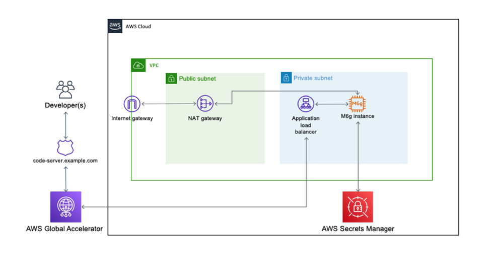
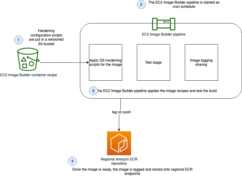
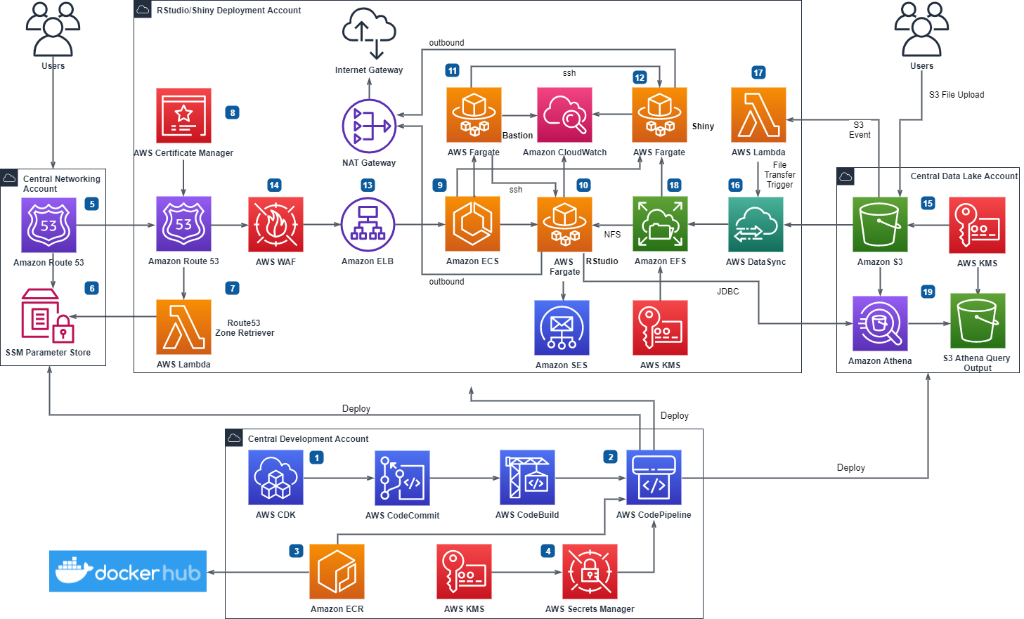
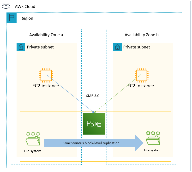
The following diagram illustrates our solution architecture.

Figure: Show the architecture of the Docker EC2 Image Builder Pipeline
We configure the Image Builder pipeline with AWS CloudFormation. Then we use Amazon Simple Storage Service (Amazon S3) as our source for the pipeline. This means that when we want to update the pipeline with a new Dockerfile, we have to update the source S3 bucket. The pipeline assumes an AWS Identity and Access Management (IAM) role that we generate later in the post. When the pipeline is run, it pulls the latest Dockerfile configuration from Amazon S3, builds a Docker image, and deploys the image to Amazon ECR. Finally, we use AWS Copilot to deploy our Docker image to Amazon ECS. For more information about Copilot, see Applications.
The style in which the Dockerfile application code was written is a personal preference. For more information, see Best practices for writing Dockerfiles.
Overview of AWS services
For this post, we use the following services:
- EC2 Image Builder – Image Builder is a fully managed AWS service that makes it easy to automate the creation, management, and deployment of customized, secure, and up-to-date server images that are pre-installed and pre-configured with software and settings to meet specific IT standards.
- Amazon ECR – Amazon ECR is an AWS managed container image registry service that is secure, scalable, and reliable.
- CodeCommit – AWS CodeCommit is a fully-managed source control service that hosts secure Git-based repositories.
- AWS KMS – Amazon Key Management Service (AWS KMS) is a fully managed service for creating and managing cryptographic keys. These keys are natively integrated with most AWS services. You use a KMS key in this post to encrypt resources.
- Amazon S3 – Amazon Simple Storage Service (Amazon S3) is an object storage service utilized for storing and encrypting data. We use Amazon S3 to store our configuration files.
- AWS CloudFormation – AWS CloudFormation allows you to use domain-specific languages or simple text files to model and provision, in an automated and secure manner, all the resources needed for your applications across all Regions and accounts. You can deploy AWS resources in a safe, repeatable manner, and automate the provisioning of infrastructure.
Prerequisites
To provision the pipeline deployment, you must have the following prerequisites:
CloudFormation templates
You use the following CloudFormation templates to deploy several resources:
- vpc.yml – Contains all the core networking configuration. It deploys the VPC, two private subnets, two public subnets, and the route tables. The private subnets utilize a NAT gateway to communicate to the internet. The public subnets have full outbound access to the internet gateway.
- kms.yml – Contains the AWS Key Management Service (AWS KMS) configuration that we use for encrypting resources. The KMS key policy is also configured in this template.
- s3-iam-config.yml – Contains the S3 bucket and IAM roles we use with our Image Builder pipeline.
- docker-image-builder.yml – Contains the configuration for the Image Builder pipeline that we use to build Docker images.
Docker Overview
Containerizing an application comes with many benefits. By containerizing an application, the application is decoupled from the underlying infrastructure, greater consistency is gained across environments, and the application can now be deployed in a loosely coupled microservice model. The lightweight nature of containers enables teams to spend less time configuring their application and more time building features that create value for their customers. To achieve these great benefits, you need reliable resources to centralize the creation and distribution of your container images. Additionally, you need to understand container fundamentals. Let’s start by reviewing a Docker base image.
In this post, we follow the multi-stage pattern for building our Docker image. With this approach, we can selectively copy artifacts from one phase to another. This allows you to remove anything not critical to the application’s function in the final image. Let’s walk through some of the logic we put into our Docker image to optimize performance and security.
Let’s begin by looking at line 15-25. Here, we are pulling down the latest amazon/aws-cli Docker image. We are leveraging this image so that we can utilize IAM credentials to clone our CodeCommit repository. In lines 15-24 we are installing and configuring our git configuration. Finally, in line 25 we are cloning our application code from our repository.
In this next section, we set environment variables, installing packages, unpack tar files, and set up a custom Java Runtime Environment (JRE). Amazon Corretto is a no-cost, multi-platform, production-ready distribution of the Open Java Development Kit (OpenJDK). One important distinction to make here is how we are utilizing RUN and ADD in the Dockerfile. By configuring our own custom JRE we can remove unnecessary modules from our image. One of our goals with building Docker images is to keep them lightweight, which is why we are taking the extra steps to ensure that we don’t add any unnecessary configuration.
Let’s take a look at the next section of the Dockerfile. Now that we have all the package that we require, we will create a working directory where we will install our demo app. After the application code is pulled down from CodeCommit, we use Maven to build our artifact.
In the following code snippet, we use FROM to begin a new stage in our build. Notice that we are using the same base as our first stage. If objects on the disk/filesystem in in the first stage stay the same, the previous stage cache can be reused. Using this pattern can greatly reduce build time.
Docker images have a single unique digest. This is a SHA-256 value and is known as the immutable identifier for the image. When changes are made to your image, through a Dockerfile update for example, a new image with a new immutable identifier is generated. The immutable identifier is pinned to prevent unexpected behaviors in code due to change or update. You can also prevent man-in-the-middle attacks by adopting this pattern. Additionally, using a SHA can mitigate the risk of having to rely on mutable tags that can be applied or changed to the wrong image by mistake. You can use the following command to check to ensure that no unintended changes occured.
docker images <input_container_image_id> --digests
Lastly, we configure our final stage, in which we create a user and group to manage our application inside the container. As this user, we copy the binaries created from our first stage. With this pattern, you can clearly see the benefit of using stages when building Docker images. Finally, we note the port that should be published with expose for the container and we define our Entrypoint, which is the instruction we use to run our container.
Deploying the CloudFormation templates
To deploy your templates, complete the following steps:
1. Create a directory where we store all of our demo code by running the following from your terminal:
mkdir awsblogrepo && cd awsblogrepo
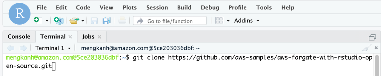
2. Clone the source code repository found in the following location:
git clone https://github.com/aws-samples/build-and-deploy-docker-images-to-aws-using-ec2-image-builder.git
You now use the AWS CLI to deploy the CloudFormation templates. Make sure to leave the CloudFormation template names as written in this post.
3. Deploy the VPC CloudFormation template:
aws cloudformation create-stack \
--stack-name vpc-config \
--template-body file://templates/vpc.yml \
--parameters file://parameters/vpc-params.json  \
--capabilities CAPABILITY_IAM \
--region us-east-1
The output should look like the following code:
{
    "StackId": "arn:aws:cloudformation:us-east-1:123456789012:stack/vpc-config/12e90fe0-76c9-11eb-9284-12717722e021"
}
4. Open the parameters/kms-params.json file and update the UserARN parameter with your account ID:
[
  {
      "ParameterKey": "KeyName",
      "ParameterValue": "DemoKey"
  },
  {
    "ParameterKey": "UserARN",
    "ParameterValue": "arn:aws:iam::<input_your_account_id>:root"
  }
]
5. Deploy the KMS key CloudFormation template:
aws cloudformation create-stack \
--stack-name kms-config \
--template-body file://templates/kms.yml \
--parameters file://parameters/kms-params.json \
--capabilities CAPABILITY_IAM \
--region us-east-1
The output should look like the following:
{
    "StackId": "arn:aws:cloudformation:us-east-1:123456789012:stack/kms-config/66a663d0-777d-11eb-ad2b-0e84b19d341f"
}
6. Open the parameters/s3-iam-config.json file and update the DemoConfigS3BucketName parameter to a unique name of your choosing:
[
  {
    "ParameterKey" : "Environment",
    "ParameterValue" : "dev"
  },
  {
    "ParameterKey": "NetworkStackName",
    "ParameterValue" : "vpc-config"
  },
  {
    "ParameterKey" : "EC2InstanceRoleName",
    "ParameterValue" : "EC2InstanceRole"
  },
  {
    "ParameterKey" : "DemoConfigS3BucketName",
    "ParameterValue" : "<input_your_unique_bucket_name>"
  },
  {
    "ParameterKey" : "KMSStackName",
    "ParameterValue" : "kms-config"
  }
]
7. Deploy the IAM role configuration template:
aws cloudformation create-stack \
--stack-name s3-iam-config \
--template-body file://templates/s3-iam-config.yml \
--parameters file://parameters/s3-iam-config.json \
--capabilities CAPABILITY_NAMED_IAM \
--region us-east-1
The output should look like the following:
{
    "StackId": "arn:aws:cloudformation:us-east-1:123456789012:stack/s3-iam-config/8b69c270-7782-11eb-a85c-0ead09d00613"
}
8. Open the parameters/kms-params.json file:
[
  {
      "ParameterKey": "KeyName",
      "ParameterValue": "DemoKey"
  },
  {
    "ParameterKey": "UserARN",
    "ParameterValue": "arn:aws:iam::1234567891012:root"
  }
]
9. Add the following values as a comma-separated list to the UserARN parameter key. Make sure to provide your AWS account ID:
arn:aws:iam::<input_your_aws_account_id>:role/EC2ImageBuilderRole
When finished, the file should look similar to the following:
[
  {
      "ParameterKey": "KeyName",
      "ParameterValue": "DemoKey"
  },
  {
    "ParameterKey": "UserARN",
    "ParameterValue": "arn:aws:iam::123456789012:role/EC2ImageBuilderRole,arn:aws:iam::123456789012:root"
  }
]
Now that the AWS KMS parameter file has been updated, you update the AWS KMS CloudFormation stack.
10. Run the following command to update the kms-config stack:
aws cloudformation update-stack \
--stack-name kms-config \
--template-body file://templates/kms.yml \
--parameters file://parameters/kms-params.json \
--capabilities CAPABILITY_IAM \
--region us-east-1
The output should look like the following:
{
    "StackId": "arn:aws:cloudformation:us-east-1:123456789012:stack/kms-config/66a663d0-777d-11eb-ad2b-0e84b19d341f"
}
11. Open the parameters/docker-image-builder-params.json file and update the ImageBuilderBucketName parameter to the bucket name you generated earlier:
[
  {
    "ParameterKey": "Environment",
    "ParameterValue": "dev"
  },
  {
      "ParameterKey": "ImageBuilderBucketName",
      "ParameterValue": "<input_your_s3_bucket_name>"
  },
  {
      "ParameterKey": "NetworkStackName",
      "ParameterValue": "vpc-config"
  },
  {
      "ParameterKey": "KMSStackName",
      "ParameterValue": "kms-config"
  },
  {
      "ParameterKey": "S3ConfigStackName",
      "ParameterValue": "s3-iam-config"
  },
  {
      "ParameterKey": "ECRName",
      "ParameterValue": "demo-ecr"
  }
]
12. Run the following commands to upload the Dockerfile and component file to S3. Make sure to update the s3 bucket name with the name you generated earlier:
aws s3 cp java/Dockerfile s3://<input_your_bucket_name>/Dockerfile && \
aws s3 cp components/component.yml s3://<input_your_bucket_name>/component.yml
The output should look like the following:
upload: java/Dockerfile to s3://demo12345/Dockerfile
upload: components/component.yml to s3://demo12345/component.yml
13. Deploy the docker-image-builder.yml template:
aws cloudformation create-stack \
--stack-name docker-image-builder-config \
--template-body file://templates/docker-image-builder.yml \
--parameters file://parameters/docker-image-builder-params.json \
--capabilities CAPABILITY_NAMED_IAM \
--region us-east-1
The output should look like the following:
{
    "StackId": "arn:aws:cloudformation:us-east-1:123456789012:stack/docker-image-builder/24317190-76f4-11eb-b879-0afa5528cb21"
}
Configure the Repository
You use AWS CodeCommit as your source control repository. You now walk through the steps of deploying our CodeCommit repository:
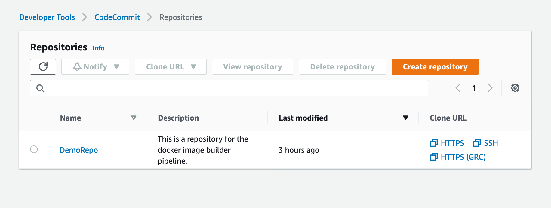
1. On the CodeCommit console, choose Repositories.
2. Locate your repository and under Clone URL, choose HTTPS.

Figure: Shows DemoRepo CodeCommit Repository
You clone this repository in the build directory you created when deploying the CloudFormation templates.
3. In your terminal, past the Git URL from the previous step and clone the repository:
git clone https://git-codecommit.us-east-1.amazonaws.com/v1/repos/DemoRepo
4. Now let’s create and push your main branch:
cd DemoRepo
git checkout -b main
touch initial.txt
git add . && git commit -m "Initial commit"
git push -u origin main
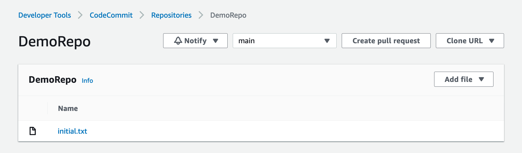
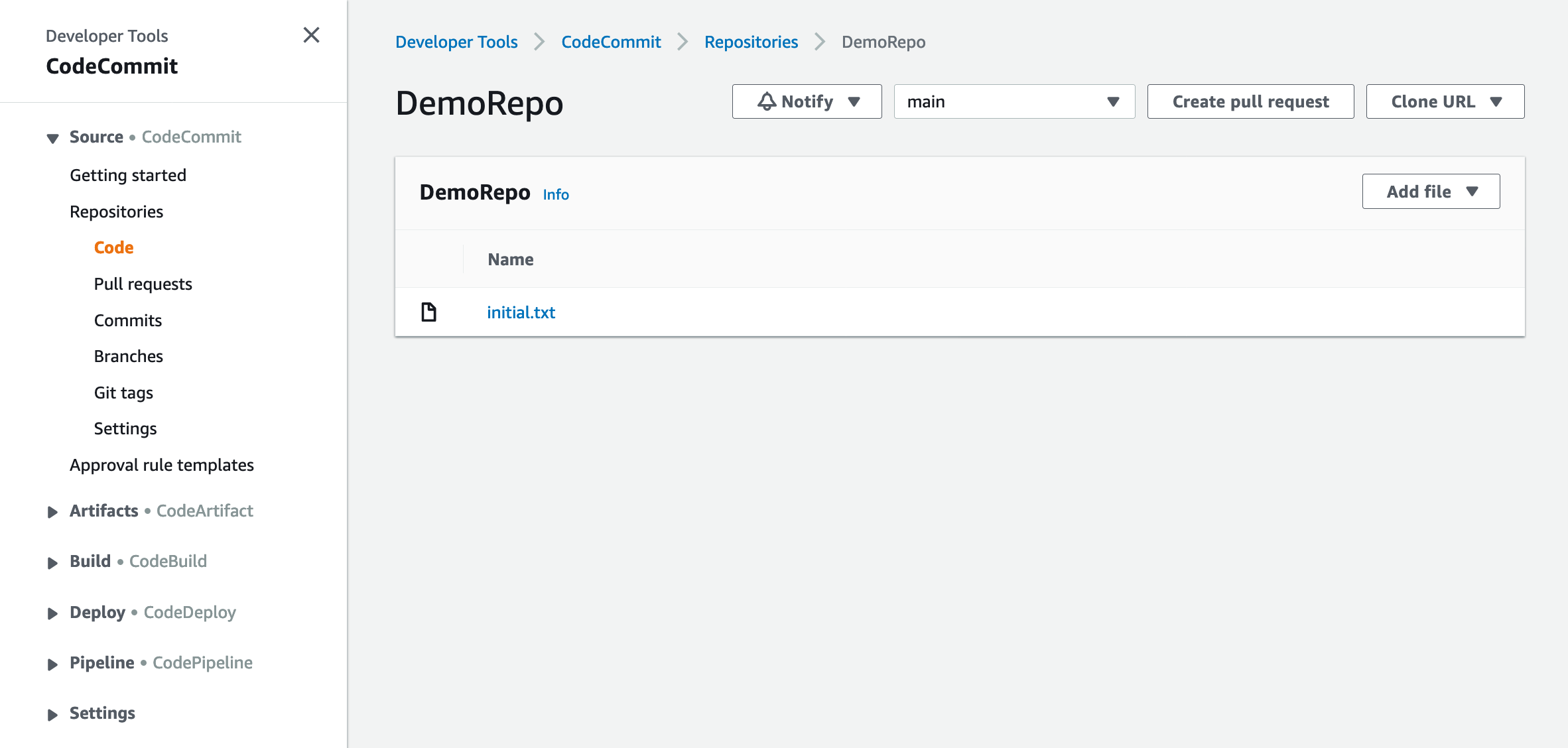
5. On the Repositories page of the CodeCommit console, choose DemoRepo.
The following screenshot shows that we have created our main branch and pushed our first commit to our repository.

Figure: Shows the DemoRepo main branch
6. Back in your terminal, create a new feature branch:
git checkout -b feature/configure-repo
7. Create the build directories:
mkdir templates; \
mkdir parameters; \
mkdir java; \
mkdir components
You now copy over the configuration files from the cloned GitHub repository to our CodeCommit repository.
8. Run the following command from the awsblogrepo directory you created earlier:
cp -r build-and-deploy-docker-images-to-aws-using-ec2-image-builder/* DemoRepo/
9. Commit and push your changes:
git add . && git commit -m "Copying config files into source control."
git push --set-upstream origin feature/configure-repo
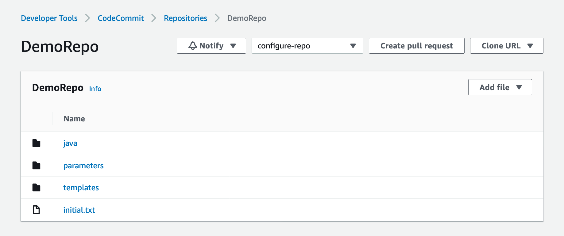
10. On the CodeCommit console, navigate to DemoRepo.
Figure: Shows the DemoRepo CodeCommit Repository
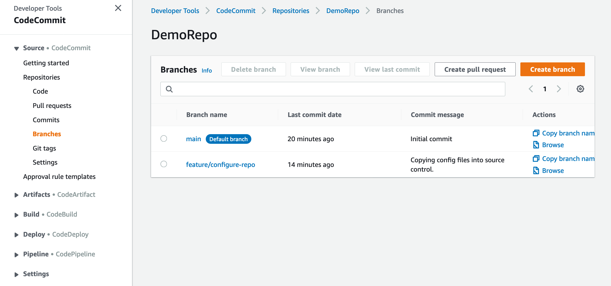
11. In the navigation pane, under Repositories, choose Branches.

Figure: Shows the DemoRepo’s code
12. Select the feature/configure-repo branch.

Figure: Shows the DemoRepo’s branches
13. Choose Create pull request.

Figure: Shows the DemoRepo code
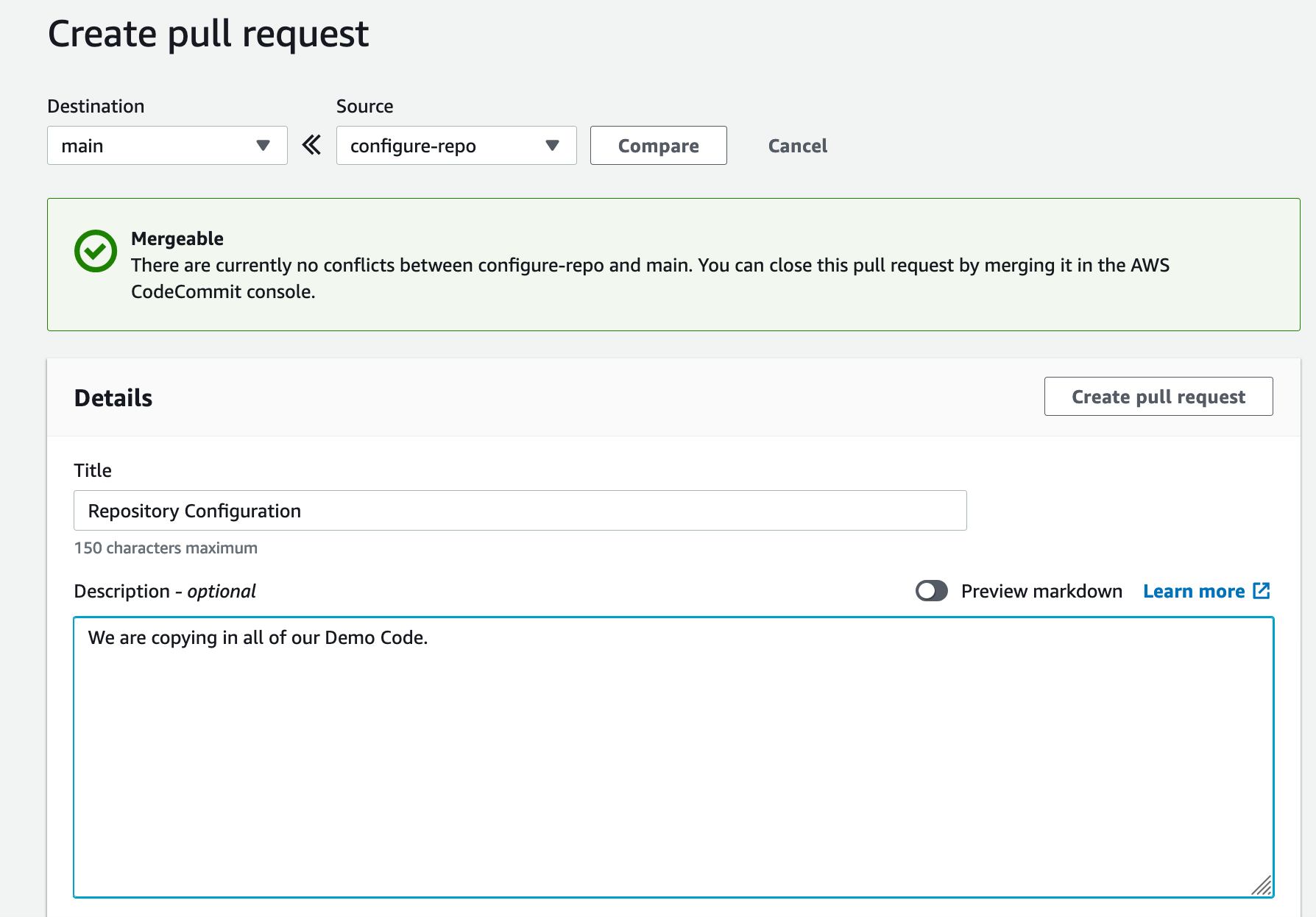
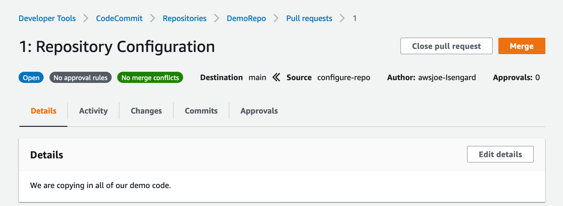
14. For Title, enter Repository Configuration.
15. For Description, enter a brief description.
16. Choose Create pull request.

Figure: Shows a pull request for DemoRepo
17. Choose Merge to merge the pull request.

Figure: Shows merge for DemoRepo pull request
Now that you have all the code copied into your CodeCommit repository, you now build an image using the Image Builder pipeline.
EC2 Image Builder Deep Dive
With Image Builder, you can build and deploy Docker images to your AWS account. Let’s look at how your Image Builder pipeline is configured.
A recipe defines the source image to use as your starting point to create a new image, along with the set of components that you add to customize your image and verify that everything is working as expected. Take note of the ParentImage property. Here, you’re declaring that the parent image that your pipeline pulls from the latest Amazon Linux image. This enables organizations to define images that they have approved to be utilized downstream by development teams. Having better control over what Docker images development teams are using improves an organization security posture while enabling the developers to have the tools they need readily available. The DockerfileTemplateUri property refers to the location of the Dockerfile that your Image Builder pipeline is deploying. Take some time to review the configuration.
Run the Image Builder Pipeline
Now you build a Docker image by running the pipeline.
1. Update your account ID and run the following command:
aws imagebuilder start-image-pipeline-execution \
--image-pipeline-arn arn:aws:imagebuilder:us-east-1:<input_your_aws_account_id>:image-pipeline/docker-image-builder-config-docker-java-container
The output should look like the following:
{
    "requestId": "87931a2e-cd74-44e9-9be1-948fec0776aa",
    "clientToken": "e0f710be-0776-43ea-a6d7-c10137a554bf",
    "imageBuildVersionArn": "arn:aws:imagebuilder:us-east-1:123456789012:image/docker-image-builder-config-container-recipe/1.0.0/1"
}
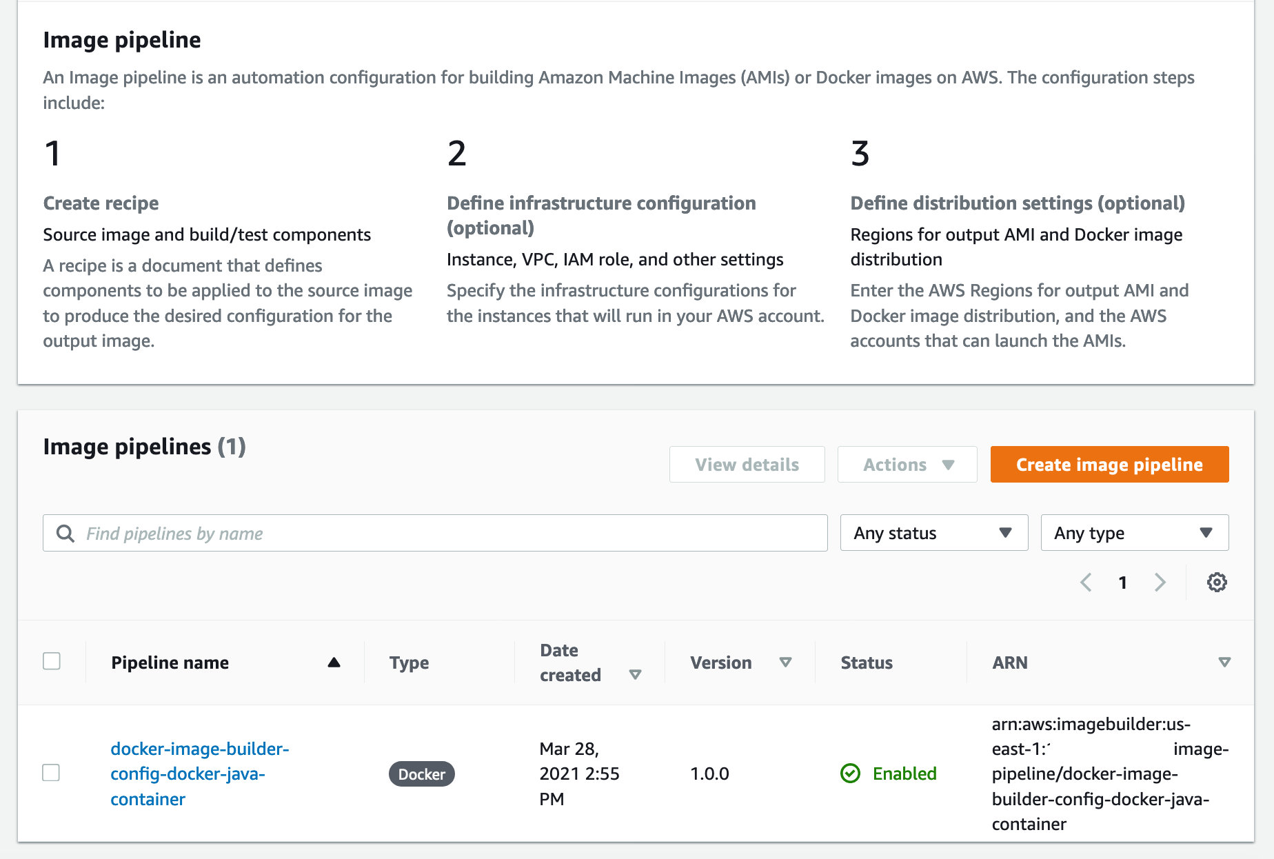
2. On the Image Builder console, choose the docker-image-builder-config-docker-java-container pipeline.

Figure: Shows EC2 Image Builder Pipeline status
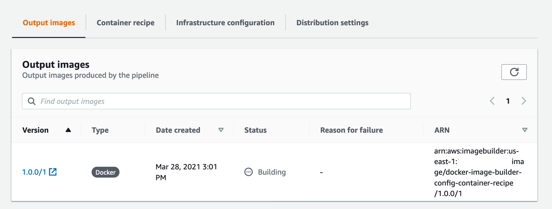
At the bottom of the page, a new Docker image is building.
3. Wait until the image status becomes Available.

Figure: Shows docker image building in EC2 Image Builder console
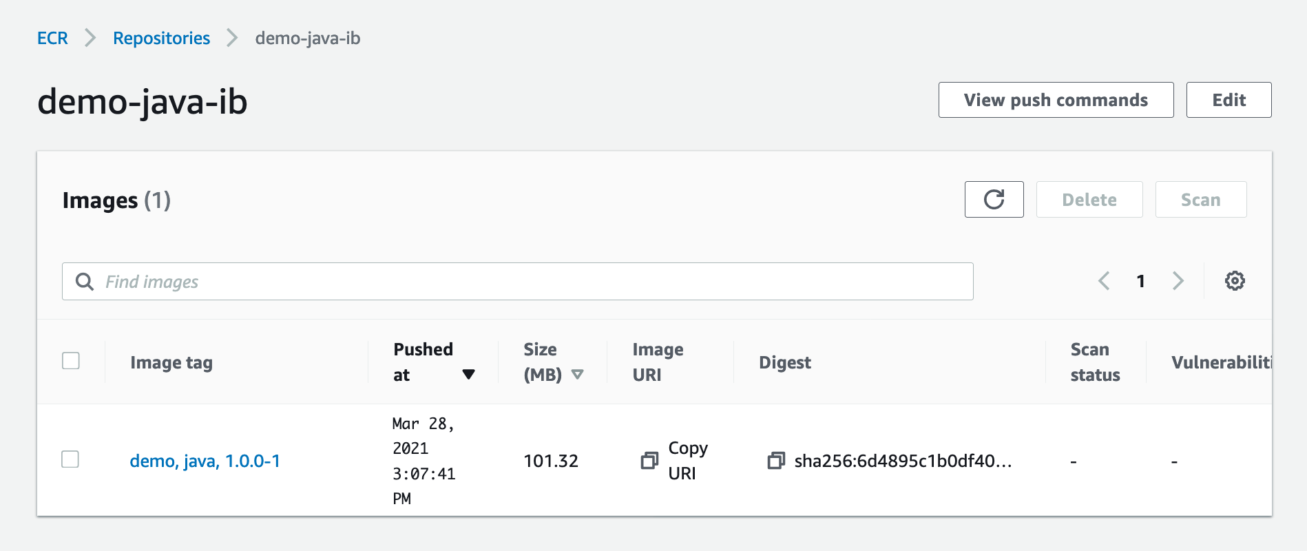
4. On the Amazon ECR console, open java-demo-ib.
The Docker image has been successfully created, tagged, and deployed to Amazon ECR from the Image Builder pipeline.

Figure: Shows demo-java-ib image in ECR
Test the Docker Image Locally
1. On the Amazon ECR console, open java-demo-ib.
2. Copy the image URI.

3. Run the following commands to authenticate to your ECR repository:
aws ecr get-login-password --region us-east-1 | docker login --username AWS --password-stdin <input_your_account_id>.dkr.ecr.us-east-1.amazonaws.com
4. Run the following command in your terminal, and update the Amazon ECR URI with the content you copied from the previous step:
docker pull <input_ecr_image_uri>
You should see output similar to the following:
1.0.0-80: Pulling from demo-java-ib
596ba82af5aa: Pull complete
6f476912a053: Pull complete
3e7162a86ef8: Pull complete
ec7d8bb8d044: Pull complete
Digest: sha256:14668cda786aa496f406062ce07087d66a14a7022023091e9b953aae0bdf2634
Status: Downloaded newer image for 123456789012.dkr.ecr.us-east-1.amazonaws.com/demo-java-ib:1.0.0-1
123456789012.dkr.ecr.us-east-1.amazonaws.com/demo-java-ib:1.0.0-1
5. Run the following command from your terminal:
docker image ls
You should see output similar to the following:
REPOSITORY                                                  TAG        IMAGE ID       CREATED          SIZE
123456789012.dkr.ecr.us-east-1.amazonaws.com/demo-java-ib   1.0.0-1   ac75e982863c   34 minutes ago   47.3MB
6. Run the following command from your terminal using the IMAGE ID value from the previous output:
docker run -dp 8090:8090 --name java_hello_world -it <docker_image_id> sh
You should see an output similar to the following:
49ea3a278639252058b55ab80c71245d9f00a3e1933a8249d627ce18c3f59ab1
7. Test your container by running the following command:
curl localhost:8090
You should see an output similar to the following:
Hello World!
8. Now that you have verified that your container is working properly, you can stop your container. Run the following command from your terminal:
docker stop java_hello_world
Conclusion
In this article, we showed how to leverage AWS services to automate the creation, management, and distribution of Docker Images. We walked through how to configure EC2 Image Builder to create and distribute Docker images. Finally, we built a Docker image using our EC2 Image Builder pipeline and tested the image locally. Thank you for reading!

Joe Keating is a Modernization Architect in Professional Services at Amazon Web Services. He works with AWS customers to design and implement a variety of solutions in the AWS Cloud. Joe enjoys cooking with a glass or two of wine and achieving mediocrity on the golf course.

Virginia Chu is a Sr. Cloud Infrastructure Architect in Professional Services at Amazon Web Services. She works with enterprise-scale customers around the globe to design and implement a variety of solutions in the AWS Cloud.

BK works as a Senior Security Architect with AWS Professional Services. He love to solve security problems for his customers, and help them feel comfortable within AWS. Outside of work, BK loves to play computer games, and go on long drives.


 Bastien Leblanc is the AWS Retail technical lead for EMEA. He works with retailers focusing on delivering exceptional end-user experience using AWS Services. With a strong background in data and analytics he helps retailers transform their business with cutting-edge AWS technologies.