Microservices structure an application as a set of independently deployable services. They speed up software development and allow architects to quickly update systems to adhere to changing business requirements.
According to best practices, the different services should be loosely coupled, organized around business capabilities, independently deployable, and owned by a single team. If applied correctly, there are multiple advantages to using microservices. However, working with microservices can also bring challenges. In this edition of Let’s Architect!, we explore the advantages, mental models, and challenges deriving from microservices with containers.
As Tim Bray said in his time with AWS, “If your application is cloud native, large scale, or distributed, and doesn’t include a messaging component, that’s probably a bug.”
This video evaluates several design patterns based on messaging and shows you how to implement them in your workloads to achieve the full capabilities of microservices. You’ll learn some fundamental application integration patterns and some of the benefits that asynchronous messaging can have over REST APIs for communication between microservices.
The scatter-gather pattern scales parallel processing across nodes and aggregates the results in a queue
Customers often cite monitoring as one of the main challenges while working with containers. Monitoring collects operational data as logs, metrics, events, and traces to identify and respond to issues quickly and minimize disruptions.
This whitepaper covers cross-service challenges in microservices, including service discovery, distributed monitoring, and auditing. You’ll learn about the role of DNS and service meshes in interservice communication and discovery and the tools available for monitoring your clusters that run containers and for logging.
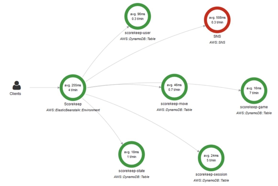
This view from AWS X-Ray shows how a request can be tracked across different services. This is implemented by taking advantage of correlation IDs
When architects deploy a new version of an application, they want to test it on a set of users before routing all the traffic to the new version. This is known as a “canary deployment.” A canary deployment can automatically switch traffic back to the old version if some inconsistencies are detected. This decreases the impact of the bug(s) introduced in the new release. For microservices, this is helpful when testing a complex distributed system because you can send a percentage of traffic to newer versions in a controlled manner.
A service mesh provides application-level networking so your services can communicate with each other across multiple types of compute infrastructure. This blog post shows how to use AWS App Mesh to implement a canary deployment strategy using AWS Step Functions for orchestrating the different steps during testing and AWS Code Pipeline for continuous delivery of each microservice.
An overview of the architecture used to create the pipeline and perform the canary deployments
Distributed architectures bring up several questions. How do we expose our APIs towards client-side applications? How do our microservices communicate?
This blog post answers these questions with a solution that uses Amazon Elastic Kubernetes Service (Amazon EKS) in conjunction with AWS App Mesh. This solution helps you manage the security and discoverability of microservices, and Kong protects your service mesh and runs side by side with your application services.
The Kong for Kubernetes architecture can be implemented using Amazon EKS and AWS App Mesh
See you next time!
See you in a couple of weeks when we discuss open source technologies on AWS!
Looking for more architecture content? AWS Architecture Center provides reference architecture diagrams, vetted architecture solutions, Well-Architected best practices, patterns, icons, and more!
Deploying global applications has many challenges, especially when accessing a database to build custom pages for end users. One example is an application using AWS Lambda@Edge. Two main challenges include performance and availability.
This blog explains how you can optimally deploy a global application with fast response times and without application changes.
The Amazon Aurora Global Database enables a single database cluster to span multiple AWS Regions by asynchronously replicating your data within subsecond timing. This provides fast, low-latency local reads in each Region. It also enables disaster recovery from Region-wide outages using multi-Region writer failover. These capabilities minimize the recovery time objective (RTO) of cluster failure, thus reducing data loss during failure. You will then be able to achieve your recovery point objective (RPO).
However, there are some implementation challenges. Most applications are designed to connect to a single hostname with atomic, consistent, isolated, and durable (ACID) consistency. But Global Aurora clusters provide reader hostname endpoints in each Region. In the primary Region, there are two endpoints, one for writes, and one for reads. To achieve strong data consistency, a global application requires the ability to:
Choose the optimal reader endpoints
Change writer endpoints on a database failover
Intelligently select the reader with the most up-to-date, freshest data
These capabilities typically require additional development.
The architecture in Figure 1 shows Aurora Global Databases primary Region in AP-SOUTHEAST-2, and secondary Regions in AP-SOUTH-1 and US-WEST-2. The Heimdall Proxy uses latency-based routing to determine the closest Reader Instance for read traffic, and redirects all write traffic to the Writer Instance. The Heimdall Configuration stores the Amazon Resource Name (ARN) of the global cluster. It automatically detects failover and cross-Region on the cluster, and directs traffic accordingly.
With an Aurora Global Database, there are two approaches to failover:
Managed planned failover. To relocate your primary database cluster to one of the secondary Regions in your Aurora global database, see Managed planned failovers with Amazon Aurora Global Database. With this feature, RPO is 0 (no data loss) and it synchronizes secondary DB clusters with the primary before making any other changes. RTO for this automated process is typically less than that of the manual failover.
Manual unplanned failover. To recover from an unplanned outage, you can manually perform a cross-Region failover to one of the secondaries in your Aurora Global Database. The RTO for this manual process depends on how quickly you can manually recover an Aurora global database from an unplanned outage. The RPO is typically measured in seconds, but this is dependent on the Aurora storage replication lag across the network at the time of the failure.
The Heimdall Proxy automatically detects Amazon Relational Database Service (RDS) / Amazon Aurora configuration changes based on the ARN of the Aurora Global cluster. Therefore, both managed planned and manual unplanned failovers are supported.
Solution benefits for global applications
Implementing the Heimdall Proxy has many benefits for global applications:
An Aurora Global Database has a primary DB cluster in one Region and up to five secondary DB clusters in different Regions. But the Heimdall Proxy deployment does not have this limitation. This allows for a larger number of endpoints to be globally deployed. Combined with Amazon Route 53 latency-based routing, new connections have a shorter establishment time. They can use connection pooling to connect to the database, which reduces overall connection latency.
SQL results are cached to the application for faster response times.
The proxy intelligently routes non-cached queries. When safe to do so, the closest (lowest latency) reader will be used. When not safe to access the reader, the query will be routed to the global writer. Proxy nodes globally synchronize their state to ensure that volatile tables are locked to provide ACID compliance.
Heimdall Data, based in the San Francisco Bay Area, is an AWS Advanced ISV partner. They have AWS Service Ready designations for Amazon RDS and Amazon Redshift. Heimdall Data offers a database proxy that offloads SQL improving database scale. Deployment does not require code changes.
Many of our customers are standardizing Kubernetes as their compute infrastructure platform for cloud and on-premises applications. Amazon EKS makes it easy to deploy containerized workloads. It provides highly available clusters and automates tasks such as patching, node provisioning, and updates.
Kubernetes uses a flat networking model that requires each pod to receive an IP address. This simplified approach enables low-friction porting of applications from virtual machines to containers but requires a significant number of IP addresses that many private VPC IPv4 networks are not equipped to handle. Some cluster administrators work around this IPv4 space limitation by installing container network plugins (CNI) that virtualize IP addresses a layer above the VPC, but this architecture limits an administrator’s ability to effectively observe and troubleshoot applications and has a negative impact on network performance at scale. Further, to communicate with internet services outside the VPC, traffic from IPv4 pods is routed through multiple network hops before reaching its destination, which adds latency and puts a strain on network engineering teams who need to maintain complex routing setups.
To avoid IP address exhaustion, minimize latency at scale, and simplify routing configuration, the solution is to use IPv6 address space.
IPv6 is not new. In 1996, I bought my first book on “IPng, Internet Protocol Next Generation”, as it was called 25 years ago. It provides a 64-bit address space, allowing 3.4 x 10^38 possible IP addresses for our devices, servers, or containers. We could assign an IPv6 address to every atom on the surface of the planet and still have enough addresses left to do another 100-plus Earths.
There are a few advantages to using Amazon EKS clusters with an IPv6 network. First, you can run more pods on one single host or subnet without the risk of exhausting all available IPv4 addresses available in your VPC. Second, it allows for lower-latency communications with other IPv6 services, running on-premises, on AWS, or on the internet, by avoiding an extra NAT hop. Third, it relieves network engineers of the burden of maintaining complex routing configurations.
Kubernetes cluster administrators can focus on migrating and scaling applications without spending efforts working around IPv4 limits. Finally, pod networking is configured so that the pods can communicate with IPv4-based applications outside the cluster, allowing you to adopt the benefits of IPv6 on Amazon EKS without requiring that all dependent services deployed across your organization are first migrated to IPv6.
As usual, I built a short demo to show you how it works.
How It Works Before I get started, I create an IPv6 VPC. I use this CDK script to create an IPv6-enabled VPC in a few minutes (thank you Angus Lees for the code). Just install CDK v2 (npm install -g aws-cdk@next) and deploy the stack (cdk bootstrap && cdk deploy).
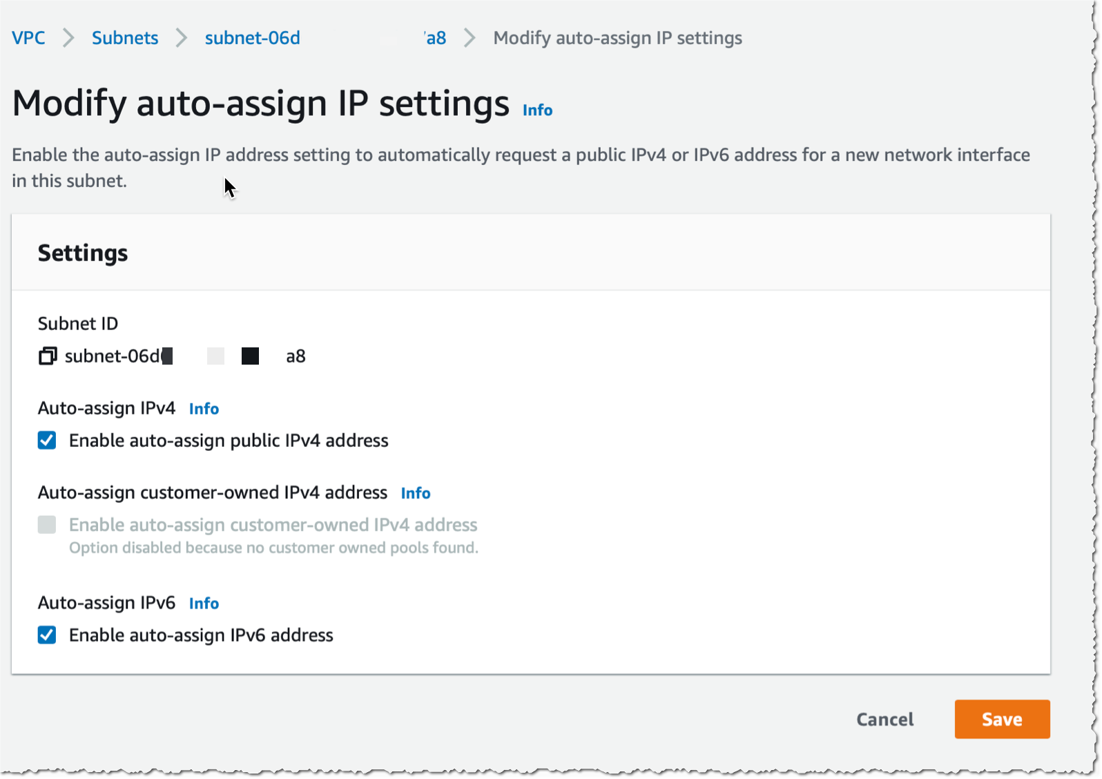
When the VPC with IPv6 is created, I use the console to configure auto-assignment of IPv6 addresses to resources deployed in the public subnets (I do this for each public subnet).
I take note of the subnet IDs created by the CDK script above (they are listed in the output of the script) and define a couple of variables I’ll use throughout the demo. I also create a cluster IAM role and a node IAM role, as described in the Amazon EKS documentation. When you already have clusters deployed, these two roles exist already.
Once the node group is created, I see two EC2 instances in the console. I use the AWS Command Line Interface (CLI) to verify that the instances received an IPv6 address:
kubectl create namespace aws-news-blog
namespace/aws-news-blog created

# sample-service.yml is available at https://docs.aws.amazon.com/eks/latest/userguide/sample-deployment.html
kubectl apply -f  sample-service.yml
service/my-service created
deployment.apps/my-deployment created

kubectl get pods -n aws-news-blog -o wide
NAME                             READY   STATUS    RESTARTS   AGE   IP                           NODE                                       NOMINATED NODE   READINESS GATES
my-deployment-5dd5dfd6b9-7rllg   1/1     Running   0          17m   2600:0000:0000:0000:405b::2   ip-10-0-1-217.us-west-2.compute.internal   <none>           <none>
my-deployment-5dd5dfd6b9-h6mrt   1/1     Running   0          17m   2600:0000:0000:0000:46f9::    ip-10-0-0-108.us-west-2.compute.internal   <none>           <none>
my-deployment-5dd5dfd6b9-mrkfv   1/1     Running   0          17m   2600:0000:0000:0000:46f9::1   ip-10-0-0-108.us-west-2.compute.internal   <none>           <none>
I take note of the IPv6 address of my pods, and try to connect it from my laptop. As my awesome service provider doesn’t provide me with an IPv6 at home yet, the connection fails. This is expected as the pods do not have an IPv4 address at all. Notice the -g option telling curl to not consider : in the IP address as the separator for the port number and -6 to tell curl to connect through IPv6 only (required when you provide curl with a DNS hostname).
curl -g -6 http://\[2600:0000:0000:35000000:46f9::1\]
curl: (7) Couldn't connect to server
To test IPv6 connectivity, I start a dual stack (IPv4 and IPv6) EC2 instance in the same VPC as the cluster. I SSH connect to the instance and try the curl command again. I see I receive the default HTML page served by nginx. IPv6 connectivity to the pod works!
curl -g -6 http://\[2600:0000:0000:35000000:46f9::1\]
<!DOCTYPE html>
<html>
<head>
<title>Welcome to nginx!</title>

... redacted for brevity ...

<p><em>Thank you for using nginx.</em></p>
</body>
</html>
If it does not work for you, verify the security group for the cluster EC2 nodes and be sure it has a rule allowing incoming connections on port TCP 80 from ::/0.
A Few Things to Remember Before I wrap up, I’d like to answer some frequent questions received from customers who have already experimented with this new capability:
IPv6 is enabled by the same VPC CNI Kubernetes plugin as the one you are using for IPv4 today. The plugin is automatically configured for IPv4 or IPv6, depending on the pod networking choice you make when you create your cluster.
IPv6 support is turned on only at cluster creation time. As of today, you can not migrate a cluster from IPv4 to IPv6. If you have an existing cluster you want to migrate, you may have to redeploy the workload to a new IPv6-based cluster and progressively migrate traffic from the IPv4 to the IPv6 cluster, such as described in this technical note.
Customers want a single and comprehensive view of the security posture of their workloads. Runtime security event monitoring is important to building secure, operationally excellent, and reliable workloads, especially in environments that run containers and container orchestration platforms. In this blog post, we show you how to use services such as AWS Security Hub and Falco, a Cloud Native Computing Foundation project, to build a continuous runtime security monitoring solution.
With the solution in place, you can collect runtime security findings from multiple AWS accounts running one or more workloads on AWS container orchestration platforms, such as Amazon Elastic Kubernetes Service (Amazon EKS) or Amazon Elastic Container Service (Amazon ECS). The solution collates the findings across those accounts into a designated account where you can view the security posture across accounts and workloads.
Solution overview
Security Hub collects security findings from other AWS services using a standardized AWS Security Findings Format (ASFF). Falco provides the ability to detect security events at runtime for containers. Partner integrations like Falco are also available on Security Hub and use ASFF. Security Hub provides a custom integrations feature using ASFF to enable collection and aggregation of findings that are generated by custom security products.
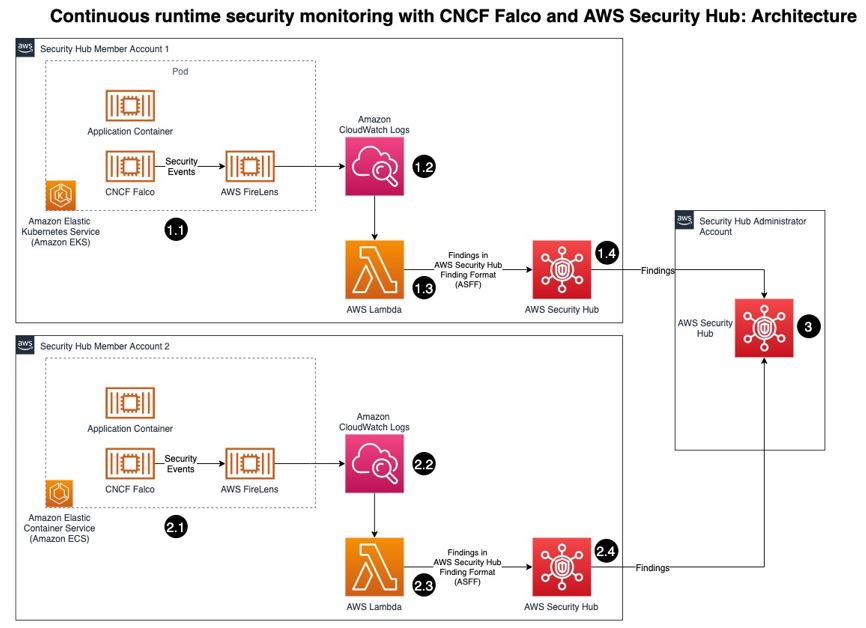
Figure 1: Architecture diagram of continuous runtime security monitoring
Here’s how the solution works, as shown in Figure 1:
An AWS account is running a workload on Amazon EKS.
Runtime security events detected by Falco for that workload are sent to CloudWatch logs using AWS FireLens.
CloudWatch logs act as the source for FireLens and a trigger for the Lambda function in the next step.
The Lambda function transforms the logs into the ASFF. These findings can now be imported into Security Hub.
The Security Hub instance that is running in the same account as the workload running on Amazon EKS stores and processes the findings provided by Lambda and provides the security posture to users of the account. This instance also acts as a member account for Security Hub.
Another AWS account is running a workload on Amazon ECS.
Runtime security events detected by Falco for that workload are sent to CloudWatch logs using AWS FireLens.
CloudWatch logs acts as the source for FireLens and a trigger for the Lambda function in the next step.
The Lambda function transforms the logs into the ASFF. These findings can now be imported into Security Hub.
The Security Hub instance that is running in the same account as the workload running on Amazon ECS stores and processes the findings provided by Lambda and provides the security posture to users of the account. This instance also acts as another member account for Security Hub.
The designated Security Hub administrator account combines the findings generated by the two member accounts, and then provides a comprehensive view of security alerts and security posture across AWS accounts. If your workloads span multiple regions, Security Hub supports aggregating findings across Regions.
Prerequisites
For this walkthrough, you should have the following in place:
Three AWS accounts.
Note: We recommend three accounts so you can experience Security Hub’s support for a multi-account setup. However, you can use a single AWS account instead to host the Amazon ECS and Amazon EKS workloads, and send findings to Security Hub in the same account. If you are using a single account, skip the following account specific-guidance. If you are integrated with AWS Organizations, the designated Security Hub administrator account will automatically have access to the member accounts.
Security Hub set up with an administrator account on one account.
Security Hub set up with member accounts on two accounts: one account to host the Amazon EKS workload, and one account to host the Amazon ECS workload.
Falco set up on the Amazon EKS and Amazon ECS clusters, with logs routed to CloudWatch Logs using FireLens. For instructions on how to do this, see:
Important: Take note of the names of the CloudWatch Logs groups, as you will need them in the next section.
AWS Cloud Development Kit (CDK) installed on the member accounts to deploy the solution that provides the custom integration between Falco and Security Hub.
Deploying the solution
In this section, you will learn how to deploy the solution and enable the CloudWatch Logs group. Enabling the CloudWatch Logs group is the trigger for running the Lambda function in both member accounts.
To deploy this solution in your own account
Clone the aws-securityhub-falco-ecs-eks-integration GitHub repository by running the following command. $git clone https://github.com/aws-samples/aws-securityhub-falco-ecs-eks-integration
Follow the instructions in the README file provided on GitHub to build and deploy the solution. Make sure that you deploy the solution to the accounts hosting the Amazon EKS and Amazon ECS clusters.
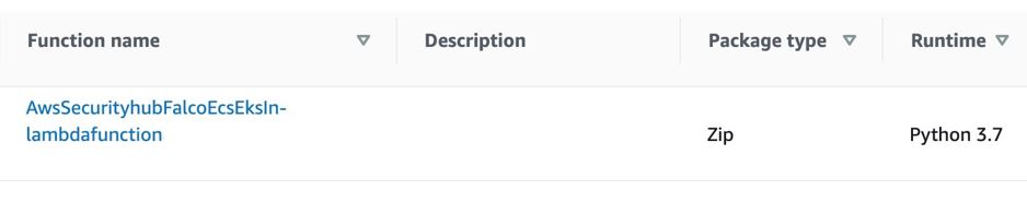
Navigate to the AWS Lambda console and confirm that you see the newly created Lambda function. You will use this function in the next section.
Figure 2: Lambda function for Falco integration with Security Hub
To enable the CloudWatch Logs group
In the AWS Management Console, select the Lambda function shown in Figure 2—AwsSecurityhubFalcoEcsEksln-lambdafunction—and then, on the Function overview screen, select + Add trigger.
On the Add trigger screen, provide the following information and then select Add, as shown in Figure 3.
Trigger configuration – From the drop-down, select CloudWatch logs.
Log group – Choose the Log group you noted in Step 4 of the Prerequisites. In our setup, the log group for the Amazon ECS and Amazon EKS clusters, deployed in separate AWS accounts, was set with the same value (falco).
Filter name – Provide a name for the filter. In our example, we used the name falco.
Filter pattern – optional – Leave this field blank.
Figure 3: Lambda function trigger – CloudWatch Log group
Repeat these steps (as applicable) to set up the trigger for the Lambda function deployed in other accounts.
Testing the deployment
Now that you’ve deployed the solution, you will verify that it’s working.
With the default rules, Falco generates alerts for activities such as:
An attempt to write to a file below the /etc folder. The /etc folder contains important system configuration files.
An attempt to open a sensitive file (such as /etc/shadow) for reading.
To test your deployment, you will attempt to perform these activities to generate Falco alerts that are reported as Security Hub findings in the same account. Then you will review the findings.
To test the deployment in member account 1
Run the following commands to trigger an alert in member account 1, which is running an Amazon EKS cluster. Replace <container_name> with your own value. kubectl exec -it <container_name> /bin/bash touch /etc/5 cat /etc/shadow > /dev/null
To see the list of findings, log in to your Security Hub admin account and navigate to Security Hub > Findings. As shown in Figure 4, you will see the alerts generated by Falco, including the Falco-generated title, and the instance where the alert was triggered.
Figure 4: Findings in Security Hub
To see more detail about a finding, check the box next to the finding. Figure 5 shows some of the details for the finding Read sensitive file untrusted.
Figure 6 shows the Resources section of this finding, that includes the instance ID of the Amazon EKS cluster node. In our example this is the Amazon Elastic Compute Cloud (Amazon EC2) instance.
To test the deployment in member account 2
Run the following commands to trigger a Falco alert in member account 2, which is running an Amazon ECS cluster. Replace <<container_id> with your own value. docker exec -it <container_id> bash touch /etc/5 cat /etc/shadow > /dev/null
As in the preceding example with member account 1, to view the findings related to this alert, navigate to your Security Hub admin account and select Findings.
To view the collated findings from both member accounts in Security Hub
In the designated Security Hub administrator account, navigate to Security Hub> Findings. The findings from both member accounts are collated in the designated Security Hub administrator account. You can use this centralized account to view the security posture across accounts and workloads. Figure 7 shows two findings, one from each member account, viewable in the Single Pane of Glass administrator account.
Figure 7: Write below /etc findings in a single view
To see more information and a link to the corresponding member account where the finding was generated, check the box next to the finding. Figure 8 shows the account detail associated with a specific finding in member account 1.
Figure 8: Write under /etc detail view in Security Hub admin account
By centralizing and enriching the findings from Falco, you can take action more quickly or perform automated remediation on the impacted resources.
Delete the Amazon EKS and Amazon ECS clusters created as part of the Prerequisites.
Conclusion
In this post, you learned how to achieve multi-account continuous runtime security monitoring for container-based workloads running on Amazon EKS and Amazon ECS. This is achieved by creating a custom integration between Falco and Security Hub.
You can extend this solution in a number of ways. For example:
You can forward findings across accounts using a single source to security information and event management (SIEM) tools such as Splunk.
You can perform automated remediation activities based on the findings generated, using Lambda.
Organizations in all industries are innovating their application stack through modernization. Developers have found that modular architecture patterns, serverless operational models, and agile development processes provide great benefits. They offer faster innovation, reduced risk, and reduction in total cost of ownership.
Security organizations must evolve and innovate as well. But security practitioners often find themselves stuck between using powerful yet inflexible open-source tools with little support, and monolithic software with expensive and restrictive licenses.
This post describes how you can use modern cloud technologies to build a scalable penetration testing platform, with no infrastructure to manage.
The penetration testing monolith
AWS operates under the shared responsibility model, where AWS is responsible for the security of the cloud, and the customer is responsible for securing workloads in the cloud. This includes validating the security of your internal and external attack surface. Following the AWS penetration testing policy, customers can run tests against their AWS accounts, except for denial of service (DoS).
A legacy model commonly involves a central server for running a scanning application among the team. The server must be powerful enough for peak load and likely runs 24/7. Common licensing for scanner software is capped on the number of targets you can scan. This model does not scale, and incurs cost when no assessments are being performed.
Penetration testers must constantly reinvent their toolkit. Many one-off tools or scripts are built during engagements when encountering a unique problem. These tools and their environments are often customized, making standardization between machines and software difficult. Building, maintaining, and testing UI/UX and platform compatibility can be expensive and difficult to scale. This often leads to these tools being discarded and the value lost when the analyst moves on to the next engagement. Later, other analysts may run into the same scenario and need to rebuild the tool all over again, resulting in duplicated effort.
Network security scanning using modern cloud infrastructure
By using modern cloud container technologies, we can redesign this monolithic architecture to one that scales to meet increased demand, yet incurs no cost when idle. Containerization provides flexibility and secure isolation.
Figure 1. Overview of the serverless security scanning architecture
Scanning task flow
This workflow is based on the architecture shown in Figure 1:
User authenticates to Amazon Cognito with their organization’s SSO.
ECS orchestrates worker nodes using AWS Fargate compute engine and initiates task.
ECS asynchronously returns the task configuration to Lambda, which sanitizes sensitive data and sends response through API Gateway.
The ECS task launches one or more containers, which run the tool.
Scan results are stored in the ephemeral storage provided by Fargate.
Final container in the ECS task copies the scan report to S3.
Now we’ll describe the different components of the architecture shown in Figure 1. Start by packaging one’s favorite tool into a container, and publish it to Amazon Elastic Container Registry (ECR). ECR provides your containers additional layers of security assurance with built-in dependency vulnerability scans.
AWS Fargate is a serverless compute engine powering Amazon ECS to orchestrate container tasks. Fargate scales up capacity to support the current load, and scales down once complete to reduce cost. By default, Fargate offers 20 GB of ephemeral storage to each ECS task for shared storage between containers as volume mounts.
Task input and output can be processed with custom code running on the serverless computing service AWS Lambda. For multi-stage Lambda functionality, you can use AWS Step Functions.
Amazon API Gateway can forward incoming requests to these Lambda functions. API Gateway provides serverless REST endpoints to handle requests processed by Lambda functions. Amazon Cognito authorizes users through API Gateway or your organization’s single-sign on (SSO) provider.
The final step of the ECS task can upload any resulting files to an Amazon S3 bucket. Amazon S3 offers industry-leading scalability, data availability, security, and performance with integration into other AWS services. This means that the results of your data can be consumed by other AWS services for processing, analytics, machine learning, and security controls.
Amazon CloudWatch Events are used to build an event-based workflow. The S3 upload initiates a CloudWatch Event, which can then invoke a Lambda function to process the file, or launch another ECS task.
This solution is completely serverless. It will scale on demand, yet cost nothing when not in use. This architecture can support anything that can be run in a container, regardless of tool function.
Network Mapper workflow
Figure 2. Network Mapper scanner task workflow
The example in Figure 2 was based on using a tool called Network Mapper, or Nmap. However, a variety of tools can be used, including nslookup/dig, Selenium, Nikto, recon-ng, SpiderFoot, Greenbone Vulnerability Manager (GVM), or OWASP ZAP. You can use anything that runs in a container! With some additional work, findings could be fed into AWS security services like AWS Security Hub, or Amazon GuardDuty. You can also use AWS Partner Network services like Splunk and Datadog, or open source frameworks like Metasploit and DefectDojo. The flexibility to add additional applications that integrate with AWS services means that this architecture can be easily deployed into a variety of AWS environments.
Remember, installation and use of software not included in an AWS-supported Amazon Machine Image (AMI) or container, falls into the customer side of the shared responsibility model. Make sure to do your due diligence in securing any software you decide to use in this or any workload. To reduce blast radius, run this in an isolated account and only provide least privilege access to targets.
Conclusion
In this blog post, we showed how to run a penetration testing workload on a modern platform, powered with serverless, and container-based services. Amazon API Gateway is the entry point for your architecture, which calls on AWS Lambda. Lambda builds a task definition to launch a fully orchestrated, on-demand container workload using AWS Fargate and Amazon ECS. The final stage of the ECS task copies the results of the scan to Amazon S3. This can be accessed by security analysts or other downstream containers, tools, or services.
We encourage you to go build this architecture in your own environment, and begin conducting your own tests! Construct your Nmap container and store it in Amazon ECR or use securecodebox/nmap, a Docker container built for the Open Web Application Security Project® (OWASP) SecureCodeBox project. Make sure to spend time securing this workload, especially when using open-source software you’re not familiar with. Now go get scanning!
More than 300,000 customers use AWS Marketplace today to find, subscribe to, and deploy third-party software packaged as Amazon Machine Images (AMIs), software-as-a-service (SaaS), and containers. Customers can find and subscribe containerized third-party applications from AWS Marketplace and deploy them in Amazon Elastic Container Service (Amazon ECS) and Amazon Elastic KubernetesService (Amazon EKS).
Many customers that run Kubernetes applications on AWS want to deploy them on-premises due to constraints, such as latency and data governance requirements. Also, once they have deployed the Kubernetes application, they need additional tools to govern the application through license tracking, billing, and upgrades.
Today, we announce AWS Marketplace for Containers Anywhere, a set of capabilities that allows AWS customers to find, subscribe to, and deploy third-party Kubernetes applications from AWS Marketplace on any Kubernetes cluster in any environment. This capability makes the AWS Marketplace more useful for customers who run containerized workloads.
With this launch, you can deploy third party Kubernetes applications to on-premises environments using Amazon EKS Anywhere or any customer self-managed Kubernetes cluster in on-premises environments or in Amazon Elastic Compute Cloud (Amazon EC2), enabling you to use a single catalog to find container images regardless of where they eventually plan to deploy.
With AWS Marketplace for Containers Anywhere, you can get the same benefits as any other products in AWS Marketplace, including consolidated billing, flexible payment options, and lower pricing for long-term contracts. You can find vetted, security-scanned, third-party Kubernetes applications, manage upgrades with a few clicks, and track all licenses and bills. You can migrate applications between any environment without purchasing duplicate licenses. After you have subscribed to an application using this feature, you can migrate your Kubernetes applications to AWS by deploying the independent software vendor (ISV) provided Helm charts onto their Kubernetes clusters on AWS without changing their licenses.
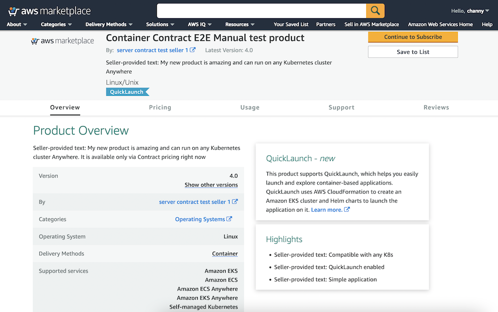
Getting Started with AWS Marketplace for Containers Anywhere You can get started by visiting AWS Marketplace. Easily search in Delivery methods in all products, then filter Helm Chart in the catalog to find Kubernetes-based applications that they can deploy on AWS and on premises.
If you chose to subscribe to your favorite product, you would select Continue to Subscribe.
Once you accept the seller’s end user license agreement (EULA), select Create Contract and Continue to Configuration.
You can configure the software deployment using the dropdowns. Once Fulfillment option and Software Version are selected, choose Continue to Launch.
To deploy on Amazon EKS, you have the option to deploy the application on a new EKS cluster or copy and paste commands into existing clusters. You can also deploy into self-managed Kubernetes in EC2 by clicking on the self-managed Kubernetes option in the supported services.
To deploy on-premises or in EC2, you can select EKS Anywhere and then take an additional step to request a license token on the AWS Marketplace launch page. You will then use commands provided by AWS Marketplace to download container images, Helm charts from the AWS Marketplace Elastic Container Registry (ECR), the service account creation, and the token to apply IAM Roles for Service Accounts on your EKS cluster.
To upgrade or renew your existing software licenses, you can go to the AWS Marketplace website for a self-service upgrade or renewal experience. You can also negotiate a private offer directly with ISVs to upgrade and renew the application. After you subscribe to the new offer, the license is automatically updated in AWS License Manager. You can view all the licenses you have purchased from AWS Marketplace using AWS License Manager, including the application capabilities you’re entitled to and the expiration date.
Launch Partners of AWS Marketplace for Containers Anywhere Here is the list of our launch partners to support an on-premises deployment option. Try them out today!
D2iQ delivers the leading independent platform for enterprise-grade Kubernetes implementations at scale and across environments, including cloud, hybrid, edge, and air-gapped.
HAProxy Technologies offers widely used software load balancers to deliver websites and applications with the utmost performance, observability, and security at any scale and in any environment.
Isovalent builds open-source software and enterprise solutions such as Cilium and eBPF solving networking, security, and observability needs for modern cloud-native infrastructure.
JFrog‘s “liquid software” mission is to power the world’s software updates through the seamless, secure flow of binaries from developers to the edge.
Kasten by Veeam provides Kasten K10, a data management platform purpose-built for Kubernetes, an easy-to-use, scalable, and secure system for backup and recovery, disaster recovery, and application mobility.
Nirmata, the creator of Kyverno, provides open source and enterprise solutions for policy-based security and automation of production Kubernetes workloads and clusters.
Palo Alto Networks, the global cybersecurity leader, is shaping the cloud-centric future with technology that is transforming the way people and organizations operate.
Prosimo‘s SaaS combines cloud networking, performance, security, AI powered observability and cost management to reduce enterprise cloud deployment complexity and risk.
Solodev is an enterprise CMS and digital ecosystem for building custom cloud apps, from content to crypto. Get access to DevOps, training, and 24/7 support—powered by AWS.
Trilio, a leader in cloud-native data protection for Kubernetes, OpenStack, and Red Hat Virtualization environments, offers solutions for backup and recovery, migration, and application mobility.
If you are interested in offering your Kubernetes application on AWS Marketplace, register and modify your product to integrate with AWS License Manager APIs using the provided AWS SDK. Integrating with AWS License Manager will allow the application to check licenses procured through AWS Marketplace.
Next, you would create a new container product on AWS Marketplace with a contract offer by submitting details of the listing, including the product information, license options, and pricing. The details would be reviewed, approved, and published by AWS Marketplace Technical Account Managers. You would then submit the new container image to AWS Marketplace ECR and add it to a newly created container product through the self-service Marketplace Management Portal. All container images are scanned for Common Vulnerabilities and Exposures (CVEs).
Finally, the product listing and container images would be published and accessible by customers on AWS Marketplace’s customer website. To learn more details about creating container products on AWS Marketplace, visit Getting started as a seller and Container-based products in the AWS documentation.
Available Now The feature of AWS Marketplace for Containers Anywhere is available now in all Regions that support AWS Marketplace. You can start using the feature directly from the product of launch partners.
Give it a try, and please send us feedback either in the AWS forum for AWS Marketplace or through your usual AWS support contacts.
Today we are announcing the launch of two features for AWS Proton. First, the most requested one in the AWS Proton open roadmap, to define and provision infrastructure using Terraform. Second, the capability to manage AWS Proton templates directly from Git repositories.
AWS Proton is a fully managed application delivery service for containers and serverless applications, announced during reinvent 2020. AWS Proton aims to help infrastructure teams automate and manage their infrastructure without impacting developer productivity. It allows developers to get the templates they need to deliver their applications without the need to involve the platform team.
When using AWS Proton, the infrastructure team needs to define the environment and the service templates. Learn more about the templates.
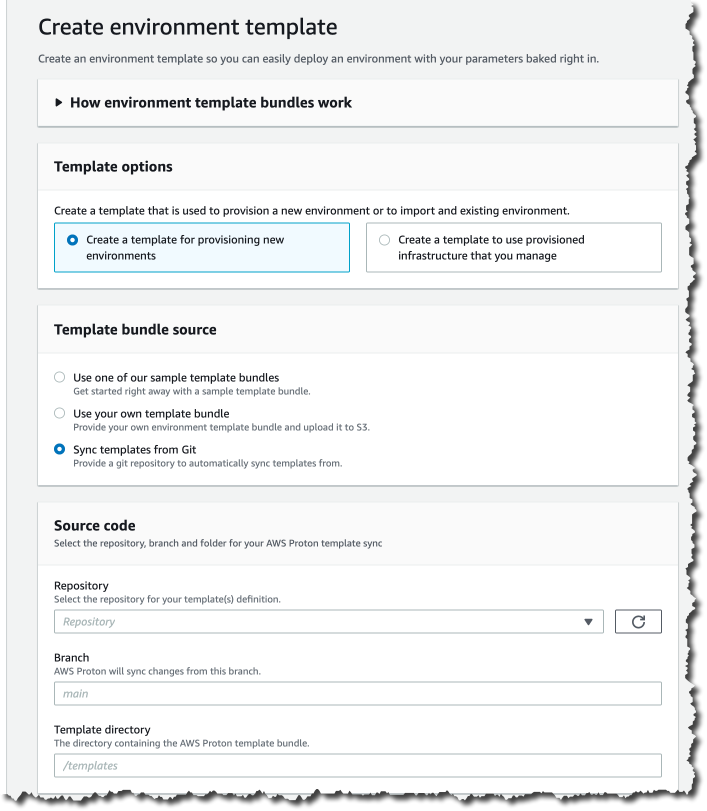
Template Sync This new feature in AWS Proton enables the platform team to push, update, and publish templates directly from their Git repositories. Now when you create a new service or environment template, you can specify a remote Git repository containing the templates. AWS Proton will automatically sync those templates and make them available for use. When there are changes to the Git repository, AWS Proton will take care of the updates.
One important advantage of using repositories and syncing the templates is that it simplifies the process of the administrators for uploading, updating, and registering the templates. This process, when done manually, can be error-prone and inconvenient. Now you can automate the process of authoring and updating the templates. Also, you can add more validations using pull requests and track the changes to the templates.
Template sync allows collaboration between the platform team and the developers. By having all the templates in a Git repository, all the collaboration tooling available in platforms like GitHub becomes available to everybody. Now developers can see all the templates, and when they want to improve them, they can just create a pull request with the changes. In addition, tools like bug trackers and features requests can be used to manage the templates.
Configuring the Repository Link To get started using template sync, you need to give AWS Proton permissions to access your repositories. For that, you need to create a link between AWS Proton and your repository.
To do this, first create a new source connection for your GitHub account. Then you need to create a new repository link from the AWS Proton. Go to the Repositories option in the side bar. Then in the Link new repository screen, use the GitHub connection that you just created and specify a repository name.
AWS Proton supports Terraform Until now, AWS CloudFormation was the only infrastructure as code (IaC) engine available in AWS Proton. Now you can define service and environment templates based on infrastructure defined using Terraform and through a pull-request-based mechanism, use Terraform to provision and keep your infrastructure updated.
Platforms teams author their IaC templates in HCL, the Terraform language, and then provision the infrastructure using Terraform Open Source. AWS Proton renders the ready-to-provision Terraform module and makes a pull request to your infrastructure repository, from where you can plan and apply the changes.
This operation is asynchronous, as AWS Proton is not the one managing the provision of infrastructure. Therefore it is important that in the process of provisioning the infrastructure, there is a step that notifies AWS Proton of the status of the deployment.
I want to show you a demo on how you can set up an environment using Terraform. For that, you will use GitHub actions to provision the Terraform infrastructure in your AWS account.
To get started with Terraform templates, first, configure the repository link as it was described before. Then you need to create a new role to give permissions to GitHub actions to perform some activities in your AWS account. You can find the AWS CloudFormationtemplate for this role here.
Create an empty GitHub repository and create a folder .github/workflows/. Create a file called terraform.yml. In that file, you need to define the GitHub actions to plan and apply the infrastructure changes. Copy the template from the terraform example file.
This template configures your AWS credentials, configures Terraform, plans the whole infrastructure, and applies the changes in the infrastructure using Terraform, and then notifies AWS Proton on the status of this process.
In addition, you need to modify the file env_config.json, which is located inside that folder. In that file, you need to add the configuration for the environment you plan to create. You can append new environments to the JSON file. In the example, the environment is called tf-test. The role is the role you created previously, and the region is the region where you want to deploy this infrastructure. Look at the example file.
Now it is time to create a new environment template in AWS Proton. You can follow the instructions in the console.
When your environment template is ready, create a new environment using the template you just created. When configuring the environment, select Provision through pull request and then configure the repository with the correct parameters.
Now, in the Environment details, you can see the Deployment status to be In progress. This will stay like this until the GitHub action finishes.
If you go to your repository, you should see a new pull request. Next to the pull request name, you will see a red cross, yellow dot, or green check. That icon depends on the status of the GitHub action. If you have a yellow dot, wait for it to turn red or green. If there is an error, you need to see what is going on inside the logs of the GitHub action.
If you see a green check on the pull request, it means that the GitHub actions has completed, and the pull request can be merged. After the pull request is merged, the infrastructure is provisioned. Go back to the Environment Details page. After a while, and once your infrastructure is provisioned, which can take some minutes depending on your template, you should see that the Deployment Status is Successful.
By the end of this demo, you have provisioned your infrastructure using AWS Proton to handle the environment templates and GitHub actions, and Terraform Open Source to provision the infrastructure in your AWS account.
Availability Terraform support is available in public preview mode.
These new features are available in the regions where AWS Proton is available: US East (Ohio), US East (N. Virginia), US West (Oregon), Asia Pacific (Tokyo), and Europe (Ireland).
To learn more about these features, visit the AWS Proton service page.
AWS App2Container is a command line tool that you can install on a server to automate the containerization of applications. This simplifies the process of migrating a single server to containers. But if you have a fleet of servers, the process of migrating all of them could be quite time-consuming. In this situation, you can automate the process using App2Container. You’ll then be able to leverage configuration management tools such as Chef, Ansible, or AWS Systems Manager. In this blog, we will illustrate an architecture to scale out App2Container, using AWS Systems Manager.
Why migrate to containers?
Organizations can move to secure, low-touch services with Containers on AWS. A container is a lightweight, standalone collection of software that includes everything needed to run an application. This can include code, runtime, system tools, system libraries, and settings. Containers provide logical isolation and will always run the same, regardless of the host environment.
If you are running a .NET application hosted on Windows Internet Information Server (IIS), when it reaches end of life (EOL) you have two options. Either migrate entire server platforms, or re-host websites on other hosting platforms. Both options require manual effort and are often too complex to implement for legacy workloads. Once workloads have been migrated, you must still perform costly ongoing patching and maintenance.
Modernize with AWS App2Container
Containers can be used for these legacy workloads via AWS App2Container. AWS App2Container is a command line interface (CLI) tool for modernizing .NET and Java applications into containerized applications. App2Container analyzes and builds an inventory of all applications running in virtual machines, on-premises, or in the cloud. App2Container reduces the need to migrate the entire server OS, and moves only the specific workloads needed.
After you select the application you want to containerize, App2Container does the following:
Packages the application artifact and identified dependencies into container images
Deploy a worker node as an Amazon Elastic Compute Cloud (Amazon EC2) instance. This will include a compatible operating system, which will take the artifacts and convert them into containers.
Install the App2Container agent on each server that you want to migrate.
Run a set of commands on each server for each application that you want to convert into a container.
Run the commands on your worker node to perform the containerization and deployment.
Following, we will introduce a way to automate App2Container to reduce the time needed to deploy and scale this functionality throughout your environment.
Scaling App2Container
AWS App2Container streamlines the process of containerizing applications on a single server. For each server you must install the App2Container agent, initialize it, run an inventory, and run an analysis. But you can save time when containerizing a fleet of machines by automation, using AWS Systems Manager. AWS Systems Manager enables you to create documents with a set of command line steps that can be applied to one or more servers.
App2Container also supports setting up a worker node that can consume the output of the App2Container analysis step. This can be deployed to the new containerized version of the applications. This allows you to follow the security best practice of least privilege. Only the worker node will have permissions to deploy containerized applications. The migrating servers will need permissions to write the analysis output into an S3 bucket.
Separate the App2Container process into two parts to use the worker node.
Analysis. This runs on the target server we are migrating. The results are output into S3.
Deployment. This runs on the worker node. It pushes the container image to Amazon ECR. It can deploy a running container to either Amazon ECS or Amazon Elastic Kubernetes Service (EKS).
As you can see in Figure 1, we need to set up an Amazon EC2 instance as the worker node, an S3 bucket for the analysis output, and two AWS Systems Manager documents. The first document is run on the target server. It will install App2Container and run the analysis steps. The second document is run on the worker node and handles the deployment of the container image. The AWS Systems Manager targets one or many hosts, enabling you to run the analysis step in parallel for multiple servers. Results and artifacts such as files or .Net assembly code, are sent to the preconfigured Amazon S3 bucket for processing as shown in Figure 2.
Figure 2. Container migration target servers
After the artifacts have been generated, a second document can be run against the worker node. This scans all files in the Amazon S3 bucket, and workloads are automatically containerized. The resulting images are pushed to Amazon ECR, as shown in Figure 3.
Figure 3. Container migration conversion
When this process is completed, you can then choose how to deploy these images, using Amazon ECS and/or Amazon EKS. Once the images and deployments are tested and the migration is completed, target servers and migration factory resources can be safely decommissioned.
This architecture demonstrates an automated approach to containerizing .NET web applications. AWS Systems Manager is used for discovery, package creation, and posting to an Amazon S3 bucket. An EC2 instance converts the package into a container so it is ready to use. The final step is to push the converted container to a scalable container repository (Amazon ECR). This way it can easily be integrated into our container platforms (ECS and EKS).
Summary
This solution offers many benefits to migrating legacy .Net based websites directly to containers. This proposed architecture is powered by AWS App2Container and automates the tooling on many targets in a secure manner. It is important to keep in mind that every customer portfolio and application requirements are unique. Therefore, it’s essential to validate and review any migration plans with business and application owners. With the right planning, engagement, and implementation, you should have a smooth and rapid journey to AWS Containers.
If you have any questions, post your thoughts in the comments section.
Monitoring is fundamental to operating an application in production, since we can only operate what we can measure and alert on. As an application evolves, or the environment grows more complex, it becomes increasingly challenging to maintain monitoring thresholds for each component, and to validate that they’re still set to an effective value. We not only want monitoring alarms to trigger when needed, but also want to minimize false positives.
Amazon DevOps Guru is an AWS service that helps you effectively monitor your application by ingesting vended metrics from Amazon CloudWatch. It learns your application’s behavior over time and then detects anomalies. Based on these anomalies, it generates insights by first combining the detected anomalies with suspected related events from AWS CloudTrail, and then providing the information to you in a simple, ready-to-use dashboard when you start investigating potential issues. Amazon DevOpsGuru makes use of the CloudWatch Containers Insights to detect issues around resource exhaustion for Amazon ECS or Amazon EKS applications. This helps in proactively detecting issues like memory leaks in your applications before they impact your users, and also provides guidance as to what the probable root-causes and resolutions might be.
This post will demonstrate how to simulate a memory leak in a container running in Amazon ECS, and have it generate a proactive insight in Amazon DevOps Guru.
Solution Overview
The following diagram shows the environment we’ll use for our scenario. The container “brickwall-maker” is preconfigured as to how quickly to allocate memory, and we have built this container image and published it to our public Amazon ECR repository. Optionally, you can build and host the docker image in your own private repository as described in step 2 & 3.
After creating the container image, we’ll utilize an AWS CloudFormation template to create an ECS Cluster and an ECS Service called “Test” with a desired count of two. This will create two tasks using our “brickwall-maker” container image. The stack will also enable Container Insights for the ECS Cluster. Then, we will enable resource coverage for this CloudFormation stack in Amazon DevOpsGuru in order to start our resource analysis.
In the AWS Cloud9 console, click Create environment, give your environment a Name, and click Next step. On the Environment settings page, change the instance type to t3.small, and click Next step. On the Review page, make sure that the Name and Instance type are set as intended, and click Create environment. The environment creation will take a few minutes. After that, the AWS Cloud9 IDE will open, and you can continue working in the terminal tab displayed in the bottom pane of the IDE.
Install the following prerequisite packages, and ensure that you have docker installed:
Change to the directory that contains the cloned repository
cd amazon-devopsguru-brickwall-maker
2. Optional : Create ECR private repository
If you want to build your own container image and host it in your own private ECR repository, create a new repository with the following command and then follow the steps to prepare your own image:
4. Launch the CloudFormation template to deploy your ECS infrastructure
To deploy your ECS infrastructure, run the following command (replace your own private ECR URL or use our public URL) in the ParameterValue) to launch the CloudFormation template :
This step lets DevOps Guru complete the baselining of the resources and benchmark the normal behavior. For this particular scenario, we recommend waiting two days before any insights are triggered.
Unlike other monitoring tools, the DevOps Guru dashboard would not present any counters or graphs. In the meantime, you can utilize CloudWatch Container Insights to monitor the cluster-level, task-level, and service-level metrics in ECS.
In the navigation pane, choose Container Insights.
Use the drop-down boxes near the top to select ECS Services as the resource type to view, then select DevOps Guru as the resource to monitor.
The performance monitoring view will show you graphs for several metrics, including “Memory Utilization”, which you can watch increasing from here. In addition, it will show the list of tasks in the lower “Task performance” pane showing the “Avg CPU” and “Avg memory” metrics for the individual tasks.
8. Review DevOps Guru insights
When DevOps Guru detects an anomaly, it generates a proactive insight with the relevant information needed to investigate the anomaly, and it will list it in the DevOps Guru Dashboard.
You can view the insights by clicking on the number of insights displayed in the dashboard. In our case, we expect insights to be shown in the “proactive insights” category on the dashboard.
Once you have opened the insight, you will see that the insight view is divided into the following sections:
Insight Overview with a basic description of the anomaly. In this case, stating that Memory Utilization is approaching limit with details of the stack that is being affected by the anomaly.
Anomalous metrics consisting of related graphs and a timeline of the predicted impact time in the future.
Relevant events with contextual information, such as changes or updates made to the CloudFormation stack’s resources in the region.
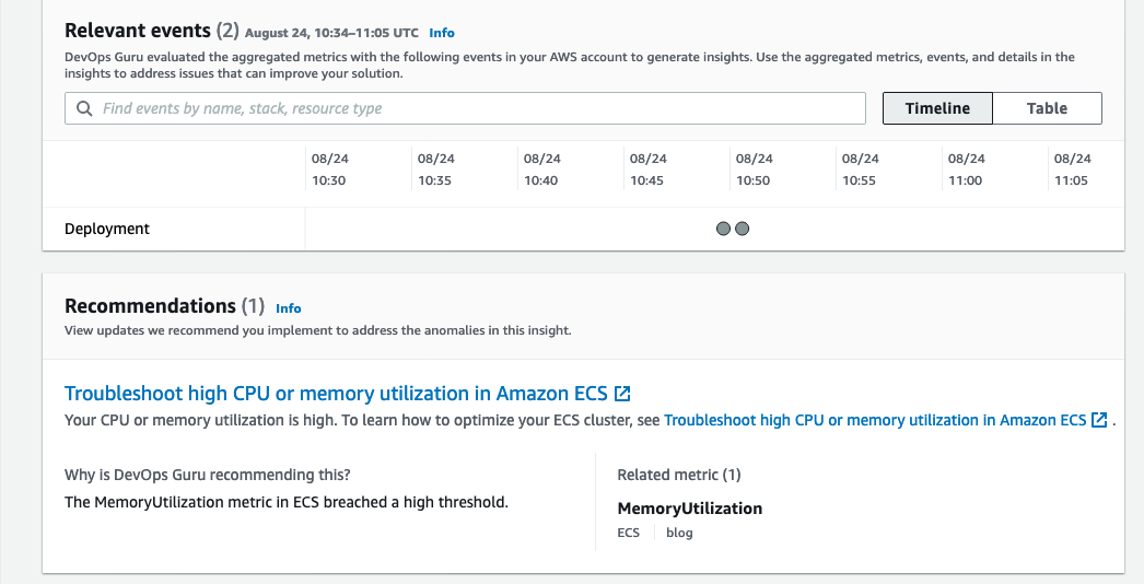
Recommendations to mitigate the issue. As seen in the following screenshot, it recommends troubleshooting High CPU or Memory Utilization in ECS along with a link to the necessary documentation.
The following screenshot illustrates an example insight detail page from DevOps Guru
Conclusion
This post describes how DevOps Guru continuously monitors resources in a particular region in your AWS account, as well as proactively helps identify problems around resource exhaustion such as running out of memory, in advance. This helps IT operators take preventative actions even before a problem presents itself, thereby preventing downtime.
Cleaning up
After walking through this post, you should clean up and un-provision the resources in order to avoid incurring any further charges.
To un-provision the CloudFormation stacks, on the AWS CloudFormation console, choose Stacks. Select the stack name, and choose Delete.
Getting the maximum scale from your database often requires fine-tuning the application. This can increase time and incur cost – effort that could be used towards other strategic initiatives. The Heimdall Proxy was designed to intelligently manage SQL connections to help you get the most out of your database.
In this blog post, we demonstrate two SQL offload features offered by this proxy:
Automated query caching
Read/Write split for improved database scale
By leveraging the solution shown in Figure 1, you can save on development costs and accelerate the onboarding of applications into production.
For ecommerce websites with high read calls and infrequent data changes, query caching can drastically improve your Amazon Relational Database Sevice (RDS) scale. You can use Amazon ElastiCache to serve results. Retrieving data from cache has a shorter access time, which reduces latency and improves I/O operations.
It can take developers considerable effort to create, maintain, and adjust TTLs for cache subsystems. The proxy technology covered in this article has features that allow for automated results caching in grid-caching chosen by the user, without code changes. What makes this solution unique is the distributed, scalable architecture. As your traffic grows, scaling is supported by simply adding proxies. Multiple proxies work together as a cohesive unit for caching and invalidation.
It can be fairly straightforward to configure a primary and read replica instance on the AWS Management Console. But it may be challenging for the developer to implement such a scale-out architecture.
Some of the issues they might encounter include:
Replication lag. A query read-after-write may result in data inconsistency due to replication lag. Many applications require strong consistency.
DNS dependencies. Due to the DNS cache, many connections can be routed to a single replica, creating uneven load distribution across replicas.
Network latency. When deploying Amazon RDS globally using the Amazon Aurora Global Database, it’s difficult to determine how the application intelligently chooses the optimal reader.
The Heimdall Proxy streamlines the ability to elastically scale out read-heavy database workloads. The Read/Write splitting supports:
ACID compliance. Determines the replication lag and know when it is safe to access a database table, ensuring data consistency.
Database load balancing. Tracks the status of each DB instance for its health and evenly distribute connections without relying on DNS.
Intelligent routing. Chooses the optimal reader to access based on the lowest latency to create local-like response times. Check out our Aurora Global Database blog.
Tornado is a modern web and mobile brokerage that empowers anyone who aspires to become a better investor.
Our engineering team was tasked to upgrade our backend such that it could handle a massive surge in traffic. With a 3-month timeline, we decided to use read replicas to reduce the load on the main database instance.
First, we migrated from Amazon RDS for PostgreSQL to Aurora for Postgres since it provided better data replication speed. But we still faced a problem – the amount of time it would take to update server code to use the read replicas would be significant. We wanted the team to stay focused on user-facing enhancements rather than server refactoring.
Enter the Heimdall Proxy: We evaluated a handful of options for a database proxy that could automatically do Read/Write splits for us with no code changes, and it became clear that Heimdall was our best option. It had the Read/Write splitting “out of the box” with zero application changes required. And it also came with database query caching built-in (integrated with Amazon ElastiCache), which promised to take additional load off the database.
Before the Tornado launch date, our load testing showed the new system handling several times more load than we were able to previously. We were using a primary Aurora Postgres instance and read replicas behind the Heimdall proxy. When the Tornado launch date arrived, the system performed well, with some background jobs averaging around a 50% hit rate on the Heimdall cache. This has really helped reduce the database load and improve the runtime of those jobs.
Using this solution, we now have a data architecture with additional room to scale. This allows us to continue to focus on enhancing the product for all our customers.
Heimdall Data, based in the San Francisco Bay Area, is an AWS Advanced Tier ISV partner. They have Amazon Service Ready designations for Amazon RDS and Amazon Redshift. Heimdall Data offers a database proxy that offloads SQL improving database scale. Deployment does not require code changes. For other proxy options, consider the Amazon RDS Proxy, PgBouncer, PgPool-II, or ProxySQL.
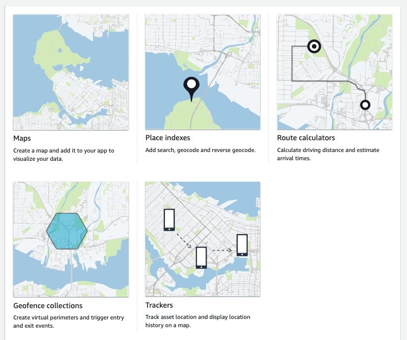
Modern location-based applications require the processing and storage of real-world assets in real-time. The recent release of Amazon Location Service and its Tracker feature makes it possible to quickly and easily build these applications on the AWS platform. Tracking real-world assets is important, but at some point when working with Location Services you will need to demo or test location-based applications without real-world assets.
Applications that track real-world assets are difficult to test and demo in a realistic setting, and it can be hard to get your hands on large amounts of real-world location data. Furthermore, not every company or individual in the early stages of developing a tracking application has access to a large fleet of test vehicles from which to derive this data.
Location data can also be considered highly sensitive, because it can be easily de-anonymized to identify individuals and movement patterns. Therefore, only a few openly accessible datasets exist and are unlikely to exhibit the characteristics required for your particular use-case.
To overcome this problem, the location-based services community has developed multiple openly available location data simulators. This blog will demonstrate how to connect one of those simulators to Amazon Location Service Tracker to test and demo your location-based services on AWS.
Walk-through
Part 1: Create a tracker in Amazon Location Service
This walkthrough will demonstrate how to get started setting up simulated data into your tracker.
Step 1: Navigate to Amazon Location Service in the AWS Console and select “Trackers“.
Step 2: On the “Trackers” screen click the orange “Create tracker“ button.
Step 3: On the “Create tracker” screen, name your tracker and make sure to reply “Yes” to the question asking you if you will only use simulated or sample data. This allows you to use the free-tier of the service.
Next, click “Create tracker” to create you tracker.
Done. You’ve created a tracker. Note the “Name” of your tracker.
Generate trips with the SharedStreets Trip-simulator
SharedStreets maintains an open-source project on GitHub – it is a probabilistic, multi-agent GPS trajectory simulator. It even creates realistic noise, and thus can be used for testing algorithms that must work under real-world conditions. Of course, the generated data is fake, so privacy is not a concern.
The trip-simulator generates files with a single GPS measurement per line. To playback those files to the Amazon Location Service Tracker, you must use a tool to parse the file; extract the GPS measurements, time measurements, and device IDs of the simulated vehicles; and send them to the tracker at the right time.
Before you start working with the playback program, the trip-simulator requires a map to simulate realistic trips. Therefore, you must download a part of OpenStreetMap (OSM). Using GeoFabrik you can download extracts at the size of states or selected cities based on the area within which you want to simulate your data.
This blog will demonstrate how to simulate a small fleet of cars in the greater Munich area. The example will be written for OS-X, but it generalizes to Linux operating systems. If you have a Windows operating system, I recommend using Windows Subsystem for Linux (WSL). Alternatively, you can run this from a Cloud9 IDE in your AWS account.
The probes.json file is the file containing the GPS probes we will playback to Amazon Location Service.
Part 2: Playback trips to Amazon Location Service
Now that you have simulated trips in the probes.json file, you can play them back in the tracker created earlier. For this, you must write only a few lines of Python code. The following steps have been neatly separated into a series of functions that yield an iterator.
Step 1: Load the probes.json file and yield each line
import json
import time
import datetime
import boto3

def iter_probes_file(probes_file_name="probes.json"):
    """Iterates a file line by line and yields each individual line."""
    with open(probes_file_name) as probes_file:
        while True:
            line = probes_file.readline()
            if not line:
                break
            yield line
Step 2: Parse the probe on each line To process the probes, you parse the JSON on each line and extract the data relevant for the playback. Note that the coordinates order is longitude, latitude in the probes.json file. This is the same order that the Location Service expects.
def parse_probes_trip_simulator(probes_iter):
    """Parses a file witch contains JSON document, one per line.
    Each line contains exactly one GPS probe. Example:
    {"properties":{"id":"RQQ-7869","time":1563123002000,"status":"idling"},"geometry":{"type":"Point","coordinates":[-86.73903753135207,36.20418779626351]}}
    The function returns the tuple (id,time,status,coordinates=(lon,lat))
    """
    for line in probes_iter:
        probe = json.loads(line)
        props = probe["properties"]
        geometry = probe["geometry"]
        yield props["id"], props["time"], props["status"], geometry["coordinates"]
Step 3: Update probe record time
The probes represent historical data. Therefore, when you playback you will need to normalize the probes recorded time to sync with the time you send the request in order to achieve the effect of vehicles moving in real-time.
This example is a single threaded playback. If the simulated playback lags behind the probe data timing, then you will be provided a warning through the code detecting the lag and outputting a warning.
The SharedStreets trip-simulator generates one probe per second. This frequency is too high for most applications, and in real-world applications you will often see frequencies of 15 to 60 seconds or even less. You must decide if you want to add another iterator for sub-sampling the data.
def update_probe_record_time(probes_iter):
    """
    Modify all timestamps to be relative to the time this function was called.
    I.e. all timestamps will be equally spaced from each other but in the future.
    """
    new_simulation_start_time_utc_ms = datetime.datetime.now().timestamp() * 1000
    simulation_start_time_ms = None
    time_delta_recording_ms = None
    for i, (_id, time_ms, status, coordinates) in enumerate(probes_iter):
        if time_delta_recording_ms is None:
            time_delta_recording_ms = new_simulation_start_time_utc_ms - time_ms
            simulation_start_time_ms = time_ms
        simulation_lag_sec = (
            (
                datetime.datetime.now().timestamp() * 1000
                - new_simulation_start_time_utc_ms
            )
            - (simulation_start_time_ms - time_ms)
        ) / 1000
        if simulation_lag_sec > 2.0 and i % 10 == 0:
            print(f"Playback lags behind by {simulation_lag_sec} seconds.")
        time_ms += time_delta_recording_ms
        yield _id, time_ms, status, coordinates
Step 4: Playback probes In this step, pack the probes into small batches and introduce the timing element into the simulation playback. The reason for placing them in batches is explained below in step 6.
def sleep(time_elapsed_in_batch_sec, last_sleep_time_sec):
    sleep_time = max(
        0.0,
        time_elapsed_in_batch_sec
        - (datetime.datetime.now().timestamp() - last_sleep_time_sec),
    )
    time.sleep(sleep_time)
    if sleep_time > 0.0:
        last_sleep_time_sec = datetime.datetime.now().timestamp()
    return last_sleep_time_sec


def playback_probes(
    probes_iter,
    batch_size=10,
    batch_window_size_sec=2.0,
):
    """
    Replays the probes in live mode.
    The function assumes, that the probes returned by probes_iter are sorted
    in ascending order with respect to the probe timestamp.
    It will either yield batches of size 10 or smaller batches if the timeout is reached.
    """
    last_probe_record_time_sec = None
    time_elapsed_in_batch_sec = 0
    last_sleep_time_sec = datetime.datetime.now().timestamp()
    batch = []
    # Creates two second windows and puts all the probes falling into
    # those windows into a batch. If the max. batch size is reached it will yield early.
    for _id, time_ms, status, coordinates in probes_iter:
        probe_record_time_sec = time_ms / 1000
        if last_probe_record_time_sec is None:
            last_probe_record_time_sec = probe_record_time_sec
        time_to_next_probe_sec = probe_record_time_sec - last_probe_record_time_sec
        if (time_elapsed_in_batch_sec + time_to_next_probe_sec) > batch_window_size_sec:
            last_sleep_time_sec = sleep(time_elapsed_in_batch_sec, last_sleep_time_sec)
            yield batch
            batch = []
            time_elapsed_in_batch_sec = 0
        time_elapsed_in_batch_sec += time_to_next_probe_sec
        batch.append((_id, time_ms, status, coordinates))
        if len(batch) == batch_size:
            last_sleep_time_sec = sleep(time_elapsed_in_batch_sec, last_sleep_time_sec)
            yield batch
            batch = []
            time_elapsed_in_batch_sec = 0
        last_probe_record_time_sec = probe_record_time_sec
    if len(batch) > 0:
        last_sleep_time_sec = sleep(time_elapsed_in_batch_sec, last_sleep_time_sec)
        yield batch
Step 5: Create the updates for the tracker
LOCAL_TIMEZONE = (
    datetime.datetime.now(datetime.timezone(datetime.timedelta(0))).astimezone().tzinfo
)

def convert_to_tracker_updates(probes_batch_iter):
    """
    Converts batches of probes in the format (id,time_ms,state,coordinates=(lon,lat))
    into batches ready for upload to the tracker.
    """
    for batch in probes_batch_iter:
        updates = []
        for _id, time_ms, _, coordinates in batch:
            # The boto3 location service client expects a datetime object for sample time
            dt = datetime.datetime.fromtimestamp(time_ms / 1000, LOCAL_TIMEZONE)
            updates.append({"DeviceId": _id, "Position": coordinates, "SampleTime": dt})
        yield updates
Step 6: Send the updates to the tracker In the update_tracker function, you use the batch_update_device_position function of the Amazon Location Service Tracker API. This lets you send batches of up to 10 location updates to the tracker in one request. Batching updates is much more cost-effective than sending one-by-one. You pay for each call to batch_update_device_position. Therefore, batching can lead to a 10x cost reduction.
def update_tracker(batch_iter, location_client, tracker_name):
    """
    Reads tracker updates from an iterator and uploads them to the tracker.
    """
    for update in batch_iter:
        response = location_client.batch_update_device_position(
            TrackerName=tracker_name, Updates=update
        )
        if "Errors" in response and response["Errors"]:
            for error in response["Errors"]:
                print(error["Error"]["Message"])
Step 7: Putting it all together The follow code is the main section that glues every part together. When using this, make sure to replace the variables probes_file_name and tracker_name with the actual probes file location and the name of the tracker created earlier.
Paste all of the code listed in steps 1 to 7 into a file called trip_playback.py, then execute
python3 trip_playback.py
This will start the playback process.
Step 8: (Optional) Tracking a device’s position updates Once the playback is running, verify that the updates are actually written to the tracker repeatedly querying the tracker for updates for a single device. Here, you will use the get_device_position function of the Amazon Location Service Tracker API to receive the last known device position.
import boto3
import time

def get_last_vehicle_position_from_tracker(
    device_id, tracker_name="your-tracker", client=boto3.client("location")
):
    response = client.get_device_position(DeviceId=device_id, TrackerName=tracker_name)
    if response["ResponseMetadata"]["HTTPStatusCode"] != 200:
        print(str(response))
    else:
        lon = response["Position"][0]
        lat = response["Position"][1]
        return lon, lat, response["SampleTime"]

if __name__ == "__main__":
    device_id = "my-device"
    tracker_name = "my-tracker"
    while True:
        lon, lat, sample_time = get_last_vehicle_position_from_tracker(
            device_id=device_id, tracker_name=tracker_name
        )
        print(f"{lon}, {lat}, {sample_time}")
        time.sleep(10)
In the example above, you must replace the tracker_name with the name of the tracker created earlier and the device_id with the ID of one of the simulation vehicles. You can find the vehicle IDs in the probes.json file created by the SharedStreets trip-simulator. If you run the above code, then you should see the following output.
AWS IoT Device Simulator
As an alternative, if you are familiar with AWS IoT, AWS has its own vehicle simulator that is part of the IoT Device Simulator solution. It lets you simulate a vehicle fleet moving on a road network. This has been described here. The simulator sends the location data to an Amazon IoT endpoint. The Amazon Location Service Developer Guide shows how to write and set-up a Lambda function to connect the IoT topic to the tracker.
The AWS IoT Device Simulator has a GUI and is a good choice for simulating a small number of vehicles. The drawback is that only a few trips are pre-packaged with the simulator and changing them is somewhat complicated. The SharedStreets Trip-simulator has much more flexibility, allowing simulations of fleets made up of a larger number of vehicles, but it has no GUI for controlling the playback or simulation.
Cleanup
You’ve created a Location Service Tracker resource. It does not incur any charges if it isn’t used. If you want to delete it, you can do so on the Amazon Location Service Tracker console.
Conclusion
This blog showed you how to use an open-source project and open-source data to generate simulated trips, as well as how to play those trips back to the Amazon Location Service Tracker. Furthermore, you have access to the AWS IoT Device Simulator, which can also be used for simulating vehicles.
Give it a try and tell us how you test your location-based applications in the comments.
This post is written by Pritam Pal, Sr EC2 Spot Specialist SA & Dan Kelly, Sr EC2 Spot GTM Specialist
Customers are using Amazon Web Services (AWS) to build CI/CD pipelines and follow DevOps best practices in order to deliver products rapidly and reliably. AWS services simplify infrastructure provisioning and management, application code deployment, software release processes automation, and application and infrastructure performance monitoring. Builders are taking advantage of low-cost, scalable compute with Amazon EC2 Spot Instances, as well as AWS Fargate Spot to build, deploy, and manage microservices or container-based workloads at a discounted price.
Amazon EC2 Spot Instances let you take advantage of unused Amazon Elastic Compute Cloud (Amazon EC2) capacity at steep discounts as compared to on-demand pricing. Fargate Spot is an AWS Fargate capability that can run interruption-tolerant Amazon Elastic Container Service (Amazon ECS) tasks at up to a 70% discount off the Fargate price. Since tasks can still be interrupted, only fault tolerant applications are suitable for Fargate Spot. However, for flexible workloads that can be interrupted, this feature enables significant cost savings over on-demand pricing.
CircleCI provides continuous integration and delivery for any platform, as well as your own infrastructure. CircleCI can automatically trigger low-cost, serverless tasks with AWS Fargate Spot in Amazon ECS. Moreover, CircleCI Orbs are reusable packages of CircleCI configuration that help automate repeated processes, accelerate project setup, and ease third-party tool integration. Currently, over 1,100 organizations are utilizing the CircleCI Amazon ECS Orb to power/run 250,000+ jobs per month.
Customers are utilizing Fargate Spot for a wide variety of workloads, such as Monte Carlo simulations and genomic processing. In this blog, I utilize a python code with the Tensorflow library that can run as a container image in order to train a simple linear model. It runs the training steps in a loop on a data batch and periodically writes checkpoints to S3. If there is a Fargate Spot interruption, then it restores the checkpoint from S3 (when a new Fargate Instance occurs) and continues training. We will deploy this on AWS ECS Fargate Spot for low-cost, serverless task deployment utilizing CircleCI.
Concepts
Before looking at the solution, let’s revisit some of the concepts we’ll be using.
Capacity Providers: Capacity providers let you manage computing capacity for Amazon ECS containers. This allows the application to define its requirements for how it utilizes the capacity. With capacity providers, you can define flexible rules for how containerized workloads run on different compute capacity types and manage the capacity scaling. Furthermore, capacity providers improve the availability, scalability, and cost of running tasks and services on Amazon ECS. In order to run tasks, the default capacity provider strategy will be utilized, or an alternative strategy can be specified if required.
AWS Fargate and AWS Fargate Spot capacity providers don’t need to be created. They are available to all accounts and only need to be associated with a cluster for utilization. When a new cluster is created via the Amazon ECS console, along with the Networking-only cluster template, the FARGATE and FARGATE_SPOT capacity providers are automatically associated with the new cluster.
CircleCI Orbs: Orbs are reusable CircleCI configuration packages that help automate repeated processes, accelerate project setup, and ease third-party tool integration. Orbs can be found in the developer hub on the CircleCI orb registry. Each orb listing has usage examples that can be referenced. Moreover, each orb includes a library of documented components that can be utilized within your config for more advanced purposes. Since the 2.0.0 release, the AWS ECS Orb supports the capacity provider strategy parameter for running tasks allowing you to efficiently run any ECS task against your new or existing clusters via Fargate Spot capacity providers.
Solution overview
Fargate Spot helps cost-optimize services that can handle interruptions like Containerized workloads, CI/CD, or Web services behind a load balancer. When Fargate Spot needs to interrupt a running task, it sends a SIGTERM signal. It is best practice to build applications capable of responding to the signal and shut down gracefully.
This walkthrough will utilize a capacity provider strategy leveraging Fargate and Fargate Spot, which mitigates risk if multiple Fargate Spot tasks get terminated simultaneously. If you’re unfamiliar with Fargate Spot, capacity providers, or capacity provider strategies, read our previous blog about Fargate Spot best practices here.
Prerequisites
Our walkthrough will utilize the following services:
CircleCI for demonstrating a CI/CD pipeline. We will utilize CircleCI Cloud Free version, which allows 2,500 free credits/week and can run 1 job at a time.
We will run a Job with CircleCI ECS Orb in order to deploy 4 ECS Tasks on Fargate and Fargate Spot. You should have the following prerequisites:
An AWS account
A GitHub account
Walkthrough
Step 1: Create AWS Keys for Circle CI to utilize.
Head to AWS IAM console, create a new user, i.e., circleci, and select only the Programmatic access checkbox. On the set permission page, select Attach existing policies directly. For the sake of simplicity, we added a managed policy AmazonECS_FullAccess to this user. However, for production workloads, employ a further least-privilege access model. Download the access key file, which will be utilized to connect to CircleCI in the next steps.
Step 2: Create an ECS Cluster, Task definition, and ECS Service
2.2 From the navigation bar, select the Region to use
2.3 In the navigation pane, choose Clusters
2.4 On the Clusters page, choose Create Cluster
2.5 Create a Networking only Cluster ( Powered by AWS Fargate)
This option lets you launch a cluster in your existing VPC to utilize for Fargate tasks. The FARGATE and FARGATE_SPOT capacity providers are automatically associated with the cluster.
2.6 Click on Update Cluster to define a default capacity provider strategy for the cluster, then add FARGATE and FARGATE_SPOT capacity providers each with a weight of 1. This ensures Tasks are divided equally among Capacity providers. Define other ratios for splitting your tasks between Fargate and Fargate Spot tasks, i.e., 1:1, 1:2, or 3:1.
2.7 Here we will create a Task Definition by using the Fargate launch type, give it a name, and specify the task Memory and CPU needed to run the task. Feel free to utilize any Fargate task definition. You can use your own code, add the code in a container, or host the container in Docker hub or Amazon ECR. Provide a name and image URI that we copied in the previous step and specify the port mappings. Click Add and then click Create.
We are also showing an example of a python code using the Tensorflow library that can run as a container image in order to train a simple linear model. It runs the training steps in a loop on a batch of data, and it periodically writes checkpoints to S3. Please find the complete code here. Utilize a Dockerfile to create a container from the code.
Sample Docker file to create a container image from the code mentioned above.
FROM ubuntu:18.04
WORKDIR /app
COPY . /app
RUN pip install -r requirements.txt EXPOSE 5000 CMD python tensorflow_checkpoint.py
Below is the Code Snippet we are using for Tensorflow to Train and Checkpoint a Training Job.
def train_and_checkpoint(net, manager):
  ckpt.restore(manager.latest_checkpoint).expect_partial()
  if manager.latest_checkpoint:
    print("Restored from {}".format(manager.latest_checkpoint))
  else:
    print("Initializing from scratch.")
  for _ in range(5000):
    example = next(iterator)
    loss = train_step(net, example, opt)
    ckpt.step.assign_add(1)
    if int(ckpt.step) % 10 == 0:
        save_path = manager.save()
        list_of_files = glob.glob('tf_ckpts/*.index')
        latest_file = max(list_of_files, key=os.path.getctime)
        upload_file(latest_file, 'pythontfckpt', object_name=None)
        list_of_files = glob.glob('tf_ckpts/*.data*')
        latest_file = max(list_of_files, key=os.path.getctime)
        upload_file(latest_file, 'pythontfckpt', object_name=None)
        upload_file('tf_ckpts/checkpoint', 'pythontfckpt', object_name=None)
2.8 Next, we will create an ECS Service, which will be used to fetch Cluster information while running the job from CircleCI. In the ECS console, navigate to your Cluster, From Services tab, then click create. Create an ECS service by choosing Cluster default strategy from the Capacity provider strategy dropdown. For the Task Definition field, choose webapp-fargate-task, which is the one we created earlier, enter a service name, set the number of tasks to zero at this point, and then leave everything else as default. Click Next step, select an existing VPC and two or more Subnets, keep everything else default, and create the service.
Step 3: GitHub and CircleCI Configuration
Create a GitHub repository, i.e., circleci-fargate-spot, and then create a .circleci folder and a config file config.yml. If you’re unfamiliar with GitHub or adding a repository, check the user guide here.
For this project, the config.yml file contains the following lines of code that configure and run your deployments.
Now, Create a CircleCI account. Choose Login with GitHub. Once you’re logged in from the CircleCI dashboard, click Add Project and add the project circleci-fargate-spot from the list shown.
When working with CircleCI Orbs, you will need the config.yml file and environment variables under Project Settings.
The config file utilizes CircleCI version 2.1 and various Orbs, i.e., AWS-ECS, AWS-CLI, and JQ. We will use a job test-fargatespot, which uses a Docker image, and we will setup the environment. In config.yml we are using the jq tool to parse JSON and fetch the ECS cluster information like VPC config, Subnets, and Security Groups needed to run an ECS task. As we are utilizing the capacity-provider-strategy, we will set the launch type parameter to an empty string.
In order to run a task, we will demonstrate how to override the default Capacity Provider strategy with Fargate & Fargate Spot, both with a weight of 1, and to divide tasks equally among Fargate & Fargate Spot. In our example, we are running 4 tasks, so 2 should run on Fargate and 2 on Fargate Spot.
Parameters like ECS_SERVICE_NAME, ECS_CLUSTER_NAME and other AWS access specific details are added securely under Project Settings and can be utilized by other jobs running within the project.
Add the following environment variables under Project Settings
AWS_ACCESS_KEY_ID – From Step 1
AWS_SECRET_ACCESS_KEY – From Step 1
AWS_DEFAULT_REGION – i.e. : – us-west-2
ECS_CLUSTER_NAME – From Step 2
ECS_SERVICE_NAME – From Step 2
SECURITY_GROUP_IDS – Security Group that will be used to run the task
Step 4: Run Job
Now in the CircleCI console, navigate to your project, choose the branch, and click Edit Config to verify that config.xml is correctly populated. Check for the ribbon at the bottom. A green ribbon means that the config file is valid and ready to run. Click Commit & Run from the top-right menu.
Click build Status to check its progress as it runs.
A successful build should look like the one below. Expand each section to see the output.
Return to the ECS console, go to the Tasks Tab, and check that 4 new tasks are running. Click each task for the Capacity provider details. Two tasks should have run with FARGATE_SPOT as a Capacity provider, and two should have run with FARGATE.
Congratulations!
You have successfully deployed ECS tasks utilizing CircleCI on AWS Fargate and Fargate Spot. If you have used any sample web applications, then please use the public IP address to see the page. If you have used the sample code that we provided, then you should see Tensorflow training jobs running on Fargate instances. If there is a Fargate Spot interruption, then it restores the checkpoint from S3 when a new Fargate Instance comes up and continues training.
Cleaning up
In order to avoid incurring future charges, delete the resources utilized in the walkthrough. Go to the ECS console and Task tab.
Delete any running Tasks.
Delete ECS cluster.
Delete the circleci user from IAM console.
Cost analysis in Cost Explorer
In order to demonstrate a cost breakdown between the tasks running on Fargate and Fargate Spot, we left the tasks running for a day. Then, we utilized Cost Explorer with the following filters and groups in order discover the savings by running Fargate Spot.
Apply a filter on Service for ECS on the right-side filter, set Group by to Usage Type, and change the time period to the specific day.
The cost breakdown demonstrates how Fargate Spot usage (indicated by “SpotUsage”) was significantly less expensive than non-Spot Fargate usage. Current Fargate Spot Pricing can be found here.
Conclusion
In this blog post, we have demonstrated how to utilize CircleCI to deploy and manage ECS tasks and run applications in a cost-effective serverless approach by using Fargate Spot.
Author bio
Pritam is a Sr. Specialist Solutions Architect on the EC2 Spot team. For the last 15 years, he evangelized DevOps and Cloud adoption across industries and verticals. He likes to deep dive and find solutions to everyday problems.
Dan is a Sr. Spot GTM Specialist on the EC2 Spot Team. He works closely with Amazon Partners to ensure that their customers can optimize and modernize their compute with EC2 Spot.
This post was contributed by Clayton Thomas, Solutions Architect, AWS WW Public Sector SLG Govtech.
Many AWS Batch users choose to store and consume their AWS Batch job container images on AWS using Amazon Elastic Container Registries (ECR). AWS Batch and Amazon Elastic Container Service (ECS) natively support pulling from Amazon ECR without any extra steps required. For those users that choose to store their container images on other container registries or Docker Hub, often times they are not publicly exposed and require authentication to pull these images. Third-party repositories may throttle the number of requests, which impedes the ability to run workloads and self-managed repositories require heavy tuning to offer the scale that Amazon ECS provides. This makes Amazon ECS the preferred solution to run workloads on AWS Batch.
While Amazon ECS allows you to configure repositoryCredentials in task definitions containing private registry credentials, AWS Batch does not expose this option in AWS Batch job definitions. AWS Batch does not provide the ability to use private registries by default but you can allow that by configuring the Amazon ECS agent in a few steps.
This post shows how to configure an AWS Batch EC2 compute environment and the Amazon ECS agent to pull your private container images from private container registries. This gives you the flexibility to use your own private and public container registries with AWS Batch.
Overview
The solution uses AWS Secrets Manager to securely store your private container registry credentials, which are retrieved on startup of the AWS Batch compute environment. This ensures that your credentials are securely managed and accessed using IAM roles and are not persisted or stored in AWS Batch job definitions or EC2 user data. The Amazon ECS agent is then configured upon startup to pull these credentials from AWS Secrets Manager. Note that this solution only supports Amazon EC2 based AWS Batch compute environments, thus AWS Fargate cannot use this solution.
Figure 1: High-level diagram showing event flow
AWS Batch uses an Amazon EC2 Compute Environment powered by Amazon ECS. This compute environment uses a custom EC2 Launch Template to configure the Amazon ECS agent to include credentials for pulling images from private registries.
An EC2 User Data script is run upon EC2 instance startup that retrieves registry credentials from AWS Secrets Manager. The EC2 instance authenticates with AWS Secrets Manager using its configured IAM instance profile, which grants temporary IAM credentials.
AWS Batch jobs can be submitted using private images that require authentication with configured credentials.
Prerequisites
For this walkthrough, you should have the following prerequisites:
An Amazon Virtual Private Cloud with private and public subnets. If you do not have a VPC, this tutorial can be followed. The AWS Batch compute environment must have connectivity to the container registry.
A container registry containing a private image. This example uses Docker Hub and assumes you have created a private repository
Registry credentials and/or an access token to authenticate with the container registry or Docker Hub.
A VPC Security Group allowing the AWS Batch compute environment egress connectivity to the container registry.
A CloudFormation template is provided to simplify setting up this example. The CloudFormation template and provided EC2 user data script can be viewed here on GitHub.
The CloudFormation template will create the following resources:
AWS Batch managed compute environment and job queue
EC2 Launch Configuration with user data script
Click the Launch Stack button to get started:
Launch the CloudFormation stack
After clicking the Launch stack button above, click Next to be presented with the following screen:
Figure 2: CloudFormation stack parameters
Fill in the required parameters as follows:
Stack Name: Give your stack a unique name.
Password: Your container registry password or Docker Hub access token. Note that both user name and password are masked and will not appear in any CF logs or output. Additionally, they are securely stored in an AWS Secrets Manager secret created by CloudFormation.
RegistryUrl: If not using Docker Hub, specify the URL of the private container registry.
User name: Your container registry user name.
SecurityGroupIDs: Select your previously created security group to assign to the example Batch compute environment.
SubnetIDs: To assign to the example Batch compute environment, select one or more VPC subnet IDs.
After entering these parameters, you can click through next twice and create the stack, which will take a few minutes to complete. Note that you must acknowledge that the template creates IAM resources on the review page before submitting.
Finally, you will be presented with a list of created AWS resources once the stack deployment finishes as shown in Figure 3 if you would like to dig deeper.
Figure 3: CloudFormation created resources
User data script contained within launch template
AWS Batch allows you to customize the compute environment in a variety of ways such as specifying an EC2 key pair, custom AMI, or an EC2 user data script. This is done by specifying an EC2 launch template before creating the Batch compute environment. For more information on Batch launch template support, see here.
Let’s take a closer look at how the Amazon ECS agent is configured upon compute environment startup to use your registry credentials.
This example script uses and installs a few tools including the AWS CLI and the open-source tool jq to retrieve and parse the previously created Secrets Manager secret. These packages are installed using the cloud-config user data type, which is part of the cloud-init packages functionality. If using the provided CloudFormation template, this script will be dynamically rendered to reference the created secret, but note that you must specify the correct Secrets Manager secret id if not using the template.
After performing a Docker login, the generated Auth JSON object is captured and passed to the Amazon ECS agent configuration to be used on AWS Batch jobs that require private images. For an explanation of Amazon ECS agent configuration options including available Amazon ECS engine Auth types, see here. This example script can be extended or customized to fit your needs but must adhere to requirements for Batch launch template user data scripts, including being in MIME multi-part archive format.
It’s worth noting that the AWS CLI automatically grabs temporary IAM credentials from the associated IAM instance profile the CloudFormation stack created in order to retrieve the Secret Manager secret values. This example assumes you created the AWS Secrets Manager secret with the default AWS managed KMS key for Secrets Manager. However, if you choose to encrypt your secret with a customer managed KMS key, make sure to specify kms:Decrypt IAM permissions for the Batch compute environment IAM role.
Submitting the AWS Batch job
Now let’s try an example Batch job that uses a private container image by creating a Batch job definition and submitting a Batch job:
Open the AWS Batch console
Navigate to the Job Definition page
Click create
Provide a unique Name for the job definition
Select the EC2 platform
Specify your private container image located in the Image field
Click create
Figure 4: Batch job definition
Now you can submit an AWS Batch job that uses this job definition:
Click on the Jobs page
Click Submit New Job
Provide a Name for the job
Select the previously created job definition
Select the Batch Job Queue created by the CloudFormation stack
Click Submit
Figure 5: Submitting a new Batch job
After submitting the AWS Batch job, it will take a few minutes for the AWS Batch Compute Environment to create resources for scheduling the job. Once that is done, you should see a SUCCEEDED status by viewing the job and filtering by AWS Batch job queue shown in Figure 6.
Figure 6: AWS Batch job succeeded
Cleaning up
To clean up the example resources, click delete for the created CloudFormation stack in the CloudFormation Console.
Conclusion
In this blog, you deployed a customized AWS Batch managed compute environment that was configured to allow pulling private container images in a secure manner. As I’ve shown, AWS Batch gives you the flexibility to use both private and public container registries. I encourage you to continue to explore the many options available natively on AWS for hosting and pulling container images. Amazon ECR or the recently launched Amazon ECR public repositories (for a deeper dive, see this blog announcement) both provide a seamless experience for container workloads running on AWS.
AWS Lambda launched support for packaging and deploying functions as container images at re:Invent 2020. In the post working with Lambda layers and extensions in container images, we demonstrated packaging Lambda Functions with layers while using container images. This post will teach you to use AWS CodePipeline to deploy docker images for microservices architecture involving multiple Lambda Functions and a common layer utilized as a separate container image. Lambda functions packaged as container images do not support adding Lambda layers to the function configuration. Alternatively, we can use a container image as a common layer while building other container images along with Lambda Functions shown in this post. Packaging Lambda functions as container images enables familiar tooling and larger deployment limits.
Here are some advantages of using container images for Lambda:
Easier dependency management and application building with container
Install native operating system packages
Install language-compatible dependencies
Consistent tool set for containers and Lambda-based applications
Utilize the same container registry to store application artifacts (Amazon ECR, Docker Hub)
Utilize the same build and pipeline tools to deploy
Tools that can inspect Dockerfile work the same
Deploy large applications with AWS-provided or third-party images up to 10 GB
Include larger application dependencies that previously were impossible
When using container images with Lambda, CodePipeline automatically detects code changes in the source repository in AWS CodeCommit, then passes the artifact to the build server like AWS CodeBuild and pushes the container images to ECR, which is then deployed to Lambda functions.
Architecture diagram
DevOps Architecture
Application Architecture
In the above architecture diagram, two architectures are combined, namely 1, DevOps Architecture and 2, Microservices Application Architecture. DevOps architecture demonstrates the use of AWS Developer services such as AWS CodeCommit, AWS CodePipeline, AWS CodeBuild along with Amazon Elastic Container Repository (ECR) and AWS CloudFormation. These are used to support Continuous Integration and Continuous Deployment/Delivery (CI/CD) for both infrastructure and application code. Microservices Application architecture demonstrates how various AWS Lambda Functions that are part of microservices utilize container images for application code. This post will focus on performing CI/CD for Lambda functions utilizing container containers. The application code used in here is a simpler version taken from Serverless DataLake Framework (SDLF). For more information, refer to the AWS Samples GitHub repository for SDLF here.
DevOps workflow
There are two CodePipelines: one for building and pushing the common layer docker image to Amazon ECR, and another for building and pushing the docker images for all the Lambda Functions within the microservices architecture to Amazon ECR, as well as deploying the microservices architecture involving Lambda Functions via CloudFormation. Common layer container image functions as a common layer in all other Lambda Function container images, therefore its code is maintained in a separate CodeCommit repository used as a source stage for a CodePipeline. Common layer CodePipeline takes the code from the CodeCommit repository and passes the artifact to a CodeBuild project that builds the container image and pushes it to an Amazon ECR repository. This common layer ECR repository functions as a source in addition to the CodeCommit repository holding the code for all other Lambda Functions and resources involved in the microservices architecture CodePipeline.
Due to all or the majority of the Lambda Functions in the microservices architecture requiring the common layer container image as a layer, any change made to it should invoke the microservices architecture CodePipeline that builds the container images for all Lambda Functions. Moreover, a CodeCommit repository holding the code for every resource in the microservices architecture is another source to that CodePipeline to get invoked. This has two sources, because the container images in the microservices architecture should be built for changes in the common layer container image as well as for the code changes made and pushed to the CodeCommit repository.
Below is the sample dockerfile that uses the common layer container image as a layer:
ARG ECR_COMMON_DATALAKE_REPO_URL
FROM ${ECR_COMMON_DATALAKE_REPO_URL}:latest AS layer
FROM public.ecr.aws/lambda/python:3.8
# Layer Code
WORKDIR /opt
COPY --from=layer /opt/ .
# Function Code
WORKDIR /var/task
COPY src/lambda_function.py .
CMD ["lambda_function.lambda_handler"]
where the argument ECR_COMMON_DATALAKE_REPO_URL should resolve to the ECR url for common layer container image, which is provided to the --build-args along with docker build command. For example:
Step 2: Change the directory to the cloned directory or extracted directory. The local code repository structure should appear as follows:
cd codepipeline-lambda-docker-images
Step 3: Deploy the CloudFormation stack used in the template file CodePipelineTemplate/codepipeline.yaml to your AWS account. This deploys the resources required for DevOps architecture involving AWS CodePipelines for common layer code and microservices architecture code. Deploy CloudFormation stacks using the AWS console by following the documentation here, providing the name for the stack (for example datalake-infra-resources) and passing the parameters while navigating the console. Furthermore, use the AWS CLI to deploy a CloudFormation stack by following the documentation here.
Step 4: When the CloudFormation Stack deployment completes, navigate to the AWS CloudFormation console and to the Outputs section of the deployed stack, then note the CodeCommit repository urls. Three CodeCommit repo urls are available in the CloudFormation stack outputs section for each CodeCommit repository. Choose one of them based on the way you want to access it. Refer to the following documentation Setting up for AWS CodeCommit. I will be using the git-remote-codecommit (grc) method throughout this post for CodeCommit access.
Step 5: Clone the CodeCommit repositories and add code:
Common Layer CodeCommit repository: Take the value of the Output for the key oCommonLayerCodeCommitHttpsGrcRepoUrl from datalake-infra-resourcesCloudFormation Stack Outputs section which looks like below:
Add contents to the cloned repository from the source code downloaded in Step 1. Copy the code from the CommonLayerCode directory and the repo contents should appear as follows:
Create the main branch and push to the remote repository
git checkout -b main
git add ./
git commit -m "Initial Commit"
git push -u origin main
Application CodeCommit repository: Take the value of the Output for the key oAppCodeCommitHttpsGrcRepoUrl from datalake-infra-resources CloudFormation Stack Outputs section which looks like below:
Clone the repository:
git clone codecommit::us-east-2://dev-AppCode
Change the directory to dev-CommonLayerCode
cd dev-AppCode
Add contents to the cloned repository from the source code downloaded in Step 1. Copy the code from the ApplicationCode directory and the repo contents should appear as follows from the root:
Create the main branch and push to the remote repository
git checkout -b main
git add ./
git commit -m "Initial Commit"
git push -u origin main
What happens now?
Now the Common Layer CodePipeline goes to the InProgress state and invokes the Common Layer CodeBuild project that builds the docker image and pushes it to the Common Layer Amazon ECR repository. The image tag utilized for the container image is the value resolved for the environment variable available in the AWS CodeBuild project CODEBUILD_RESOLVED_SOURCE_VERSION. This is the CodeCommit git Commit Id in this case. For example, if the CommitId in CodeCommit is f1769c87, then the pushed docker image will have this tag along with latest
buildspec.yaml files appears as follows:
version: 0.2
phases:
  install:
    runtime-versions:
      docker: 19
  pre_build:
    commands:
      - echo Logging in to Amazon ECR...
      - aws --version
      - $(aws ecr get-login --region $AWS_DEFAULT_REGION --no-include-email)
      - REPOSITORY_URI=$ECR_COMMON_DATALAKE_REPO_URL
      - COMMIT_HASH=$(echo $CODEBUILD_RESOLVED_SOURCE_VERSION | cut -c 1-7)
      - IMAGE_TAG=${COMMIT_HASH:=latest}
  build:
    commands:
      - echo Build started on `date`
      - echo Building the Docker image...
      - docker build -t $REPOSITORY_URI:latest .
      - docker tag $REPOSITORY_URI:latest $REPOSITORY_URI:$IMAGE_TAG
  post_build:
    commands:
      - echo Build completed on `date`
      - echo Pushing the Docker images...
      - docker push $REPOSITORY_URI:latest
      - docker push $REPOSITORY_URI:$IMAGE_TAG
Now the microservices architecture CodePipeline goes to the InProgress state and invokes all of the application image builder CodeBuild project that builds the docker images and pushes them to the Amazon ECR repository.
To improve the performance, every docker image is built in parallel within the codebuild project. The buildspec.yaml executes the build.sh script. This has the logic to build docker images required for each Lambda Function part of the microservices architecture. The docker images used for this sample architecture took approximately 4 to 5 minutes when the docker images were built serially. After switching to parallel building, it took approximately 40 to 50 seconds.
#!/bin/bash
set -eu
set -o pipefail

RESOURCE_PREFIX="${RESOURCE_PREFIX:=stg}"
AWS_DEFAULT_REGION="${AWS_DEFAULT_REGION:=us-east-1}"
ACCOUNT_ID=$(aws sts get-caller-identity --query Account --output text 2>&1)
ECR_COMMON_DATALAKE_REPO_URL="${ECR_COMMON_DATALAKE_REPO_URL:=$ACCOUNT_ID.dkr.ecr.$AWS_DEFAULT_REGION.amazonaws.com\/$RESOURCE_PREFIX-common-datalake-library}"
pids=()
pids1=()

PROFILE='new-profile'
aws configure --profile $PROFILE set credential_source EcsContainer

aws --version
$(aws ecr get-login --region $AWS_DEFAULT_REGION --no-include-email)
COMMIT_HASH=$(echo $CODEBUILD_RESOLVED_SOURCE_VERSION | cut -c 1-7)
BUILD_TAG=build-$(echo $CODEBUILD_BUILD_ID | awk -F":" '{print $2}')
IMAGE_TAG=${BUILD_TAG:=COMMIT_HASH:=latest}

cd dockerfiles;
mkdir ../logs
function pwait() {
    while [ $(jobs -p | wc -l) -ge $1 ]; do
        sleep 1
    done
}

function build_dockerfiles() {
    if [ -d $1 ]; then
        directory=$1
        cd $directory
        echo $directory
        echo "---------------------------------------------------------------------------------"
        echo "Start creating docker image for $directory..."
        echo "---------------------------------------------------------------------------------"
            REPOSITORY_URI=$ACCOUNT_ID.dkr.ecr.$AWS_DEFAULT_REGION.amazonaws.com/$RESOURCE_PREFIX-$directory
            docker build --build-arg ECR_COMMON_DATALAKE_REPO_URL=$ECR_COMMON_DATALAKE_REPO_URL . -t $REPOSITORY_URI:latest -t $REPOSITORY_URI:$IMAGE_TAG -t $REPOSITORY_URI:$COMMIT_HASH
            echo Build completed on `date`
            echo Pushing the Docker images...
            docker push $REPOSITORY_URI
        cd ../
        echo "---------------------------------------------------------------------------------"
        echo "End creating docker image for $directory..."
        echo "---------------------------------------------------------------------------------"
    fi
}

for directory in *; do
   echo "------Started processing code in $directory directory-----"
   build_dockerfiles $directory 2>&1 1>../logs/$directory-logs.log | tee -a ../logs/$directory-logs.log &
   pids+=($!)
   pwait 20
done

for pid in "${pids[@]}"; do
  wait "$pid"
done

cd ../cfn/
function build_cfnpackages() {
    if [ -d ${directory} ]; then
        directory=$1
        cd $directory
        echo $directory
        echo "---------------------------------------------------------------------------------"
        echo "Start packaging cloudformation package for $directory..."
        echo "---------------------------------------------------------------------------------"
        aws cloudformation package --profile $PROFILE --template-file template.yaml --s3-bucket $S3_BUCKET --output-template-file packaged-template.yaml
        echo "Replace the parameter 'pEcrImageTag' value with the latest built tag"
        echo $(jq --arg Image_Tag "$IMAGE_TAG" '.Parameters |= . + {"pEcrImageTag":$Image_Tag}' parameters.json) > parameters.json
        cat parameters.json
        ls -al
        cd ../
        echo "---------------------------------------------------------------------------------"
        echo "End packaging cloudformation package for $directory..."
        echo "---------------------------------------------------------------------------------"
    fi
}

for directory in *; do
    echo "------Started processing code in $directory directory-----"
    build_cfnpackages $directory 2>&1 1>../logs/$directory-logs.log | tee -a ../logs/$directory-logs.log &
    pids1+=($!)
    pwait 20
done

for pid in "${pids1[@]}"; do
  wait "$pid"
done

cd ../logs/
ls -al
for f in *; do
  printf '%s\n' "$f"
  paste /dev/null - < "$f"
done

cd ../
The function build_dockerfiles() loops through each directory within the dockerfiles directory and runs the docker build command in order to build the docker image. The name for the docker image and then the ECR repository is determined by the directory name in which the DockerFile is used from. For example, if the DockerFile directory is routing-lambda and the environment variables take the below values,
Then REPOSITORY_URI becomes 0123456789.dkr.ecr.us-east-2.amazonaws.com/dev-routing-lambda And the docker image is pushed to this resolved REPOSITORY_URI. Similarly, docker images for all other directories are built and pushed to Amazon ECR.
Important Note: The ECR repository names match the directory names where the DockerFiles exist and was already created as part of the CloudFormation template codepipeline.yaml that was deployed in step 3. In order to add more Lambda Functions to the microservices architecture, make sure that the ECR repository name added to the new repository in the codepipeline.yaml template matches the directory name within the AppCode repository dockerfiles directory.
Every docker image is built in parallel in order to save time. Each runs as a separate operating system process and is pushed to the Amazon ECR repository. This also controls the number of processes that could run in parallel by setting a value for the variable pwait within the loop. For example, if pwait 20, then the maximum number of parallel processes is 20 at a given time. The image tag for all docker images used for Lambda Functions is constructed via the CodeBuild BuildId, which is available via environment variable $CODEBUILD_BUILD_ID, in order to ensure that a new image gets a new tag. This is required for CloudFormation to detect changes and update Lambda Functions with the new container image tag.
Once every docker image is built and pushed to Amazon ECR in the CodeBuild project, it builds every CloudFormation package by uploading all local artifacts to Amazon S3 via AWS Cloudformation package CLI command for the templates available in its own directory within the cfn directory. Moreover, it updates every parameters.json file for each directory with the ECR image tag to the parameter value pEcrImageTag. This is required for CloudFormation to detect changes and update the Lambda Function with the new image tag.
After this, the CodeBuild project will output the packaged CloudFormation templates and parameters files as an artifact to AWS CodePipeline so that it can be deployed via AWS CloudFormation in further stages. This is done by first creating a ChangeSet and then deploying it at the next stage.
Testing the microservices architecture
As stated above, the sample application utilized for microservices architecture involving multiple Lambda Functions is a modified version of the Serverless Data Lake Framework. The microservices architecture CodePipeline deployed every AWS resource required to run the SDLF application via AWS CloudFormation stages. As part of SDLF, it also deployed a set of DynamoDB tables required for the applications to run. I utilized the meteorites sample for this, thereby the DynamoDb tables should be added with the necessary data for the application to run for this sample.
Utilize the AWS console to write data to the AWS DynamoDb Table. For more information, refer to this documentation. The sample json files are in the utils/DynamoDbConfig/ directory.
1. Add the record below to the octagon-Pipelines-dev DynamoDB table:
Now upload the sample json files to the raw s3 bucket. The raw S3 bucket name can be obtained in the output of the common-cloudformation stack deployed as part of the microservices architecture CodePipeline. Navigate to the CloudFormation console in the region where the CodePipeline was deployed and locate the stack with the name common-cloudformation, navigate to the Outputs section, and then note the output bucket name with the key oCentralBucket. Navigate to the Amazon S3 Bucket console and locate the bucket for oCentralBucket, create two path directories named engineering/meteorites, and upload every sample json file to this directory. Meteorites sample json files are available in the utils/meteorites-test-json-files directory of the previously cloned repository. Wait a few minutes and then navigate to the stage bucket noted from the common-cloudformation stack output name oStageBucket. You can see json files converted into csv in pre-stage/engineering/meteorites folder in S3. Wait a few more minutes and then navigate to the post-stage/engineering/meteorites folder in the oStageBucket to see the csv files converted to parquet format.
Cleanup
Navigate to the AWS CloudFormation console, note the S3 bucket names from the common-cloudformation stack outputs, and empty the S3 buckets. Refer to Emptying the Bucket for more information.
Delete the CloudFormation stacks in the following order: 1. Common-Cloudformation 2. stagea 3. stageb 4. sdlf-engineering-meteorites Then delete the infrastructure CloudFormation stack datalake-infra-resources deployed using the codepipeline.yaml template. Refer to the following documentation to delete CloudFormation Stacks: Deleting a stack on the AWS CloudFormation console or Deleting a stack using AWS CLI.
Conclusion
This method lets us use CI/CD via CodePipeline, CodeCommit, and CodeBuild, along with other AWS services, to automatically deploy container images to Lambda Functions that are part of the microservices architecture. Furthermore, we can build a common layer that is equivalent to the Lambda layer that could be built independently via its own CodePipeline, and then build the container image and push to Amazon ECR. Then, the common layer container image Amazon ECR functions as a source along with its own CodeCommit repository which holds the code for the microservices architecture CodePipeline. Having two sources for microservices architecture codepipeline lets us build every docker image. This is due to a change made to the common layer docker image that is referred to in other docker images, and another source that holds the code for other microservices including Lambda Function.
About the Author
Kirankumar Chandrashekar is a Sr.DevOps consultant at AWS Professional Services. He focuses on leading customers in architecting DevOps technologies. Kirankumar is passionate about DevOps, Infrastructure as Code, and solving complex customer issues. He enjoys music, as well as cooking and traveling.
In this blog post, I demonstrate how to implement service-to-service authorization using OAuth 2.0 access tokens for microservice APIs hosted on Amazon Elastic Kubernetes Service (Amazon EKS). A common use case for OAuth 2.0 access tokens is to facilitate user authorization to a public facing application. Access tokens can also be used to identify and authorize programmatic access to services with a system identity instead of a user identity. In service-to-service authorization, OAuth 2.0 access tokens can be used to help protect your microservice API for the entire development lifecycle and for every application layer. AWS Well Architected recommends that you validate security at all layers, and by incorporating access tokens validated by the microservice, you can minimize the potential impact if your application gateway allows unintended access. The solution sample application in this post includes access token security at the outset. Access tokens are validated in unit tests, local deployment, and remote cluster deployment on Amazon EKS. Amazon Cognito is used as the OAuth 2.0 token issuer.
Benefits of using access token security with microservice APIs
Some of the reasons you should consider using access token security with microservices include the following:
Access tokens provide production grade security for microservices in non-production environments, and are designed to ensure consistent authentication and authorization and protect the application developer from changes to security controls at a cluster level.
They enable service-to-service applications to identify the caller and their permissions.
Access tokens are short-lived credentials that expire, which makes them preferable to traditional API gateway long-lived API keys.
You get better system integration with a web or mobile interface, or application gateway, when you include token validation in the microservice at the outset.
Overview of solution
In the solution described in this post, the sample microservice API is deployed to Amazon EKS, with an Application Load Balancer (ALB) for incoming traffic. Figure 1 shows the application architecture on Amazon Web Services (AWS).
Figure 1: Application architecture
The application client shown in Figure 1 represents a service-to-service workflow on Amazon EKS, and shows the following three steps:
The application client requests an access token from the Amazon Cognito user pool token endpoint.
The access token is forwarded to the ALB endpoint over HTTPS when requesting the microservice API, in the bearer token authorization header. The ALB is configured to use IP Classless Inter-Domain Routing (CIDR) range filtering.
The microservice deployed to Amazon EKS validates the access token using JSON Web Key Sets (JWKS), and enforces the authorization claims.
Walkthrough
The walkthrough in this post has the following steps:
Amazon EKS cluster setup
Amazon Cognito configuration
Microservice OAuth 2.0 integration
Unit test the access token claims
Deployment of microservice on Amazon EKS
Integration tests for local and remote deployments
Prerequisites
For this walkthrough, you should have the following prerequisites in place:
A basic familiarity with Kotlin or Java, and frameworks such as Quarkus or Spring
A Unix terminal
Set up
Amazon EKS is the target for your microservices deployment in the sample application. Use the following steps to create an EKS cluster. If you already have an EKS cluster, you can skip to the next section: To set up the AWS Load Balancer Controller. The following example creates an EKS cluster in the Asia Pacific (Singapore) ap-southeast-1 AWS Region. Be sure to update the Region to use your value.
To create an EKS cluster with eksctl
In your Unix editor, create a file named eks-cluster-config.yaml, with the following cluster configuration:
Create the cluster by using the following eksctl command:
eksctl create cluster -f eks-cluster-config.yaml
Allow 10–15 minutes for the EKS control plane and managed nodes creation. eksctl will automatically add the cluster details in your kubeconfig for use with kubectl.
Validate your cluster node status as “ready” with the following command
kubectl get nodes
Create the demo namespace to host the sample application by using the following command:
kubectl create namespace demo
With the EKS cluster now up and running, there is one final setup step. The ALB for inbound HTTPS traffic is created by the AWS Load Balancer Controller directly from the EKS cluster using a Kubernetes Ingress resource.
To set up the AWS Load Balancer Controller
Follow the installation steps to deploy the AWS Load Balancer Controller to Amazon EKS.
An Ingress resource defines the ALB configuration. You customize the ALB by using annotations. Create a file named alb.yml, and add resource definition as follows, replacing the inbound IP CIDR with your values:
Deploy the Ingress resource with kubectl to create the ALB by using the following command:
kubectl apply -f alb.yml
After a few moments, you should see the ALB move from status provisioning to active, with an auto-generated public DNS name.
Validate the ALB DNS name and the ALB is in active status by using the following command:
kubectl -n demo describe ingress alb-ingress
To alias your host, in this case gateway.example.com with the ALB, create a Route 53 alias record. The remote API is now accessible using your Route 53 alias, for example: https://gateway.example.com/api/demo/*
The ALB that you created will only allow incoming HTTPS traffic on port 443, and restricts incoming traffic to known source IP addresses. If you want to share the ALB across multiple microservices, you can add the alb.ingress.kubernetes.io/group.name annotation. To help protect the application from common exploits, you should add an annotation to bind AWS Web Application Firewall (WAFv2) ACLs, including rate-limiting options for the microservice.
Configure the Amazon Cognito user pool
To manage the OAuth 2.0 client credential flow, you create an Amazon Cognito user pool. Use the following procedure to create the Amazon Cognito user pool in the console.
In the top-right corner of the page, choose Create a user pool.
Provide a name for your user pool, and choose Review defaults to save the name.
Review the user pool information and make any necessary changes. Scroll down and choose Create pool.
Note down your created Pool Id, because you will need this for the microservice configuration.
Next, to simulate the client in subsequent tests, you will create three app clients: one for read permission, one for write permission, and one for the microservice.
To create Amazon Cognito app clients
In the left navigation pane, under General settings, choose App clients.
On the right pane, choose Add an app client.
Enter the App client name as readClient.
Leave all other options unchanged.
Choose Create app client to save.
Choose Add another app client, and add an app client with the name writeClient, then repeat step 5 to save.
Choose Add another app client, and add an app client with the name microService. Clear Generate Client Secret, as this isn’t required for the microservice. Leave all other options unchanged. Repeat step 5 to save.
Note down the App client id created for the microService app client, because you will need it to configure the microservice.
You now have three app clients: readClient, writeClient, and microService.
With the read and write clients created, the next step is to create the permission scope (role), which will be subsequently assigned.
To create read and write permission scopes (roles) for use with the app clients
In the left navigation pane, under App integration, choose Resource servers.
On the right pane, choose Add a resource server.
Enter the name Gateway for the resource server.
For the Identifier enter your host name, in this case https://gateway.example.com.Figure 2 shows the resource identifier and custom scopes for read and write role permission.
Figure 2: Resource identifier and custom scopes
In the first row under Scopes, for Name enter demo.read, and for Description enter Demo Read role.
In the second row under Scopes, for Name enter demo.write, and for Description enter Demo Write role.
Choose Save changes.
You have now completed configuring the custom role scopes that will be bound to the app clients. To complete the app client configuration, you will now bind the role scopes and configure the OAuth2.0 flow.
To configure app clients for client credential flow
In the left navigation pane, under App Integration, select App client settings.
On the right pane, the first of three app clients will be visible.
Scroll to the readClient app client and make the following selections:
For Enabled Identity Providers, select Cognito User Pool.
Under OAuth 2.0, for Allowed OAuth Flows, select Client credentials.
Under OAuth 2.0, under Allowed Custom Scopes, select the demo.read scope.
Leave all other options blank.
Scroll to the writeClient app client and make the following selections:
For Enabled Identity Providers, select Cognito User Pool.
Under OAuth 2.0, for Allowed OAuth Flows, select Client credentials.
Under OAuth 2.0, under Allowed Custom Scopes, select the demo.write scope.
Leave all other options blank.
Scroll to the microService app client and make the following selections:
For Enabled Identity Providers, select Cognito User Pool.
Under OAuth 2.0, for Allowed OAuth Flows, select Client credentials.
Under OAuth 2.0, under Allowed Custom Scopes, select the demo.read scope.
Leave all other options blank.
Figure 3 shows the app client configured with the client credentials flow and custom scope—all other options remain blank
Figure 3: App client configuration
Your Amazon Cognito configuration is now complete. Next you will integrate the microservice with OAuth 2.0.
Microservice OAuth 2.0 integration
For the server-side microservice, you will use Quarkus with Kotlin. Quarkus is a cloud-native microservice framework with strong Kubernetes and AWS integration, for the Java Virtual Machine (JVM) and GraalVM. GraalVM native-image can be used to create native executables, for fast startup and low memory usage, which is important for microservice applications.
On the top left, you can modify the Group, Artifact and Build Tool to your preference, or accept the defaults.
In the Pick your extensions search box, select each of the following extensions:
RESTEasy JAX-RS
RESTEasy Jackson
Kubernetes
Container Image Jib
OpenID Connect
Choose Generate your application to download your application as a .zip file.
Quarkus permits low-code integration with an identity provider such as Amazon Cognito, and is configured by the project application.properties file.
To configure application properties to use the Amazon Cognito IDP
Edit the application.properties file in your quick start project:
src/main/resources/application.properties
Add the following properties, replacing the variables with your values. Use the cognito-pool-id and microservice App client id that you noted down when creating these Amazon Cognito resources in the previous sections, along with your Region.
The Kotlin code sample that follows verifies the authenticated principle by using the @Authenticated annotation filter, which performs JSON Web Key Set (JWKS) token validation. The JWKS details are cached, adding nominal latency to the application performance.
The access token claims are auto-filtered by the @RolesAllowed annotation for the custom scopes, read and write. The protected methods are illustrations of a microservice API and how to integrate this with one to two lines of code.
import io.quarkus.security.Authenticated
import javax.annotation.security.RolesAllowed
import javax.enterprise.context.RequestScoped
import javax.ws.rs.*

@Authenticated
@RequestScoped
@Path("/api/demo")
class DemoResource {

    @GET
    @Path("protectedRole/{name}")
    @RolesAllowed("https://gateway.example.com/demo.read")
    fun protectedRole(@PathParam(value = "name") name: String) = mapOf("protectedAPI" to "true", "paramName" to name)


    @POST
    @Path("protectedUpload")
    @RolesAllowed("https://gateway.example.com/demo.write")
    fun protectedDataUpload(values: Map<String, String>) = "Received: $values"

}
Unit test the access token claims
For the unit tests you will test three scenarios: unauthorized, forbidden, and ok. The @TestSecurity annotation injects an access token with the specified role claim using the Quarkus test security library. To include access token security in your unit test only requires one line of code, the @TestSecurity annotation, which is a strong reason to include access token security validation upfront in your development. The unit test code in the following example maps to the protectedRole method for the microservice via the uri /api/demo/protectedRole, with an additional path parameter sample-username to be returned by the method for confirmation.
Deploying the microservice to Amazon EKS is the same as deploying to any upstream Kubernetes-compliant installation. You declare your application resources in a manifest file, and you deploy a container image of your application to your container registry. You can do this in a similar low-code manner with the Quarkus Kubernetes extension, which automatically generates the Kubernetes deployment and service resources at build time. The Quarkus Container Image Jib extension to automatically build the container image and deploys the container image to Amazon Elastic Container Registry (ECR), without the need for a Dockerfile.
Amazon ECR setup
Your microservice container image created during the build process will be published to Amazon Elastic Container Registry (Amazon ECR) in the same Region as the target Amazon EKS cluster deployment. Container images are stored in a repository in Amazon ECR, and in the following example uses a convention for the repository name of project name and microservice name. The first command that follows creates the Amazon ECR repository to host the microservice container image, and the second command obtains login credentials to publish the container image to Amazon ECR.
To set up the application for Amazon ECR integration
In the AWS CLI, create an Amazon ECR repository by using the following command. Replace the project name variable with your parent project name, and replace the microservice name with the microservice name.
Obtain an ECR authorization token, by using your IAM principal with the following command. Replace the variables with your values for the AWS account ID and Region.
After the application re-build, you should now have a container image deployed to Amazon ECR in your region with the following name [project-group]/[project-name]. The Quarkus build will give an error if the push to Amazon ECR failed.
Now, you can deploy your application to Amazon EKS, with kubectl from the following build path:
kubectl apply -f build/kubernetes/kubernetes.yml
Integration tests for local and remote deployments
The following environment assumes a Unix shell: either MacOS, Linux, or Windows Subsystem for Linux (WSL 2).
How to obtain the access token from the token endpoint
Obtain the access token for the application client by using the Amazon Cognito OAuth 2.0 token endpoint, and export an environment variable for re-use. Replace the variables with your Amazon Cognito pool name, and AWS Region respectively.
To generate the client credentials in the required format, you need the Base64 representation of the app client client-id:client-secret. There are many tools online to help you generate a Base64 encoded string. Export the following environment variables, to avoid hard-coding in configuration or scripts.
You can use curl to post to the token endpoint, and obtain an access token for the read and write app client respectively. You can pass grant_type=client_credentials and the custom scopes as appropriate. If you pass an incorrect scope, you will receive an invalid_grant error. The Unix jq tool extracts the access token from the JSON string. If you do not have the jq tool installed, you can use your relevant package manager (such as apt-get, yum, or brew), to install using sudo [package manager] install jq.
The following shell commands obtain the access token associated with the read or write scope. The client credentials are used to authorize the generation of the access token. An environment variable stores the read or write access token for future use. Update the scope URL to your host, in this case gateway.example.com.
If the curl commands are successful, you should see the access tokens in the environment variables by using the following echo commands:
echo $access_token_read
echo $access_token_write
For more information or troubleshooting, see TOKEN Endpoint in the Amazon Cognito Developer Guide.
Test scope with automation script
Now that you have saved the read and write access tokens, you can test the API. The endpoint can be local or on a remote cluster. The process is the same, all that changes is the target URL. The simplicity of toggling the target URL between local and remote is one of the reasons why access token security can be integrated into the full development lifecycle.
To perform integration tests in bulk, use a shell script that validates the response code. The example script that follows validates the API call under three test scenarios, the same as the unit tests:
If no valid access token is passed: 401 (unauthorized) response is expected.
A valid access token is passed, but with an incorrect role claim: 403 (forbidden) response is expected.
A valid access token and valid role-claim is passed: 200 (ok) response with content-type of application/json expected.
Name the following script, demo-api.sh. For each API method in the microservice, you duplicate these three tests, but for the sake of brevity in this post, I’m only showing you one API method here, protectedRole.
Test the microservice API against the access token claims
Run the script for a local host deployment on http://localhost:8080, and on the remote EKS cluster, in this case https://gateway.example.com.
If everything works as expected, you will have demonstrated the same test process for local and remote deployments of your microservice. Another advantage of creating a security test automation process like the one demonstrated, is that you can also include it as part of your continuous integration/continuous delivery (CI/CD) test automation.
The test automation script accepts the microservice host URL as a parameter (the default is local), referencing the stored access tokens from the environment variables. Upon error, the script will exit with the error code. To test the remote EKS cluster, use the following command, with your host URL, in this case gateway.example.com.
./demo-api.sh https://<gateway.example.com>
Expected output:
Test 401-unauthorized: No access token for /api/demo/protectedRole/{name}
Test 403-forbidden: Incorrect role/custom-scope for /api/demo/protectedRole/{name}
Test 200-ok: Correct role for /api/demo/protectedRole/{name}
  Output: {"protectedAPI":"true","paramName":"sample-username"}!200!application/json
Best practices for a well architected production service-to-service client
For elevated security in alignment with AWS Well Architected, it is recommend to use AWS Secrets Manager to hold the client credentials. Separating your credentials from the application permits credential rotation without the requirement to release a new version of the application or modify environment variables used by the service. Access to secrets must be tightly controlled because the secrets contain extremely sensitive information. Secrets Manager uses AWS Identity and Access Management (IAM) to secure access to the secrets. By using the permissions capabilities of IAM permissions policies, you can control which users or services have access to your secrets. Secrets Manager uses envelope encryption with AWS KMS customer master keys (CMKs) and data key to protect each secret value. When you create a secret, you can choose any symmetric customer managed CMK in the AWS account and Region, or you can use the AWS managed CMK for Secrets Manager aws/secretsmanager.
Access tokens can be configured on Amazon Cognito to expire in as little as 5 minutes or as long as 24 hours. To avoid unnecessary calls to the token endpoint, the application client should cache the access token and refresh close to expiry. In the Quarkus framework used for the microservice, this can be automatically performed for a client service by adding the quarkus-oidc-client extension to the application.
Cleaning up
To avoid incurring future charges, delete all the resources created.
To delete the EKS cluster, and the associated Application Load Balancer, follow the steps described in Deleting a cluster in the Amazon EKS User Guide.
This post has focused on the last line of defense, the microservice, and the importance of a layered security approach throughout the development lifecycle. Access token security should be validated both at the application gateway and microservice for end-to-end API protection.
As an additional layer of security at the application gateway, you should consider using Amazon API Gateway, and the inbuilt JWT authorizer to perform the same API access token validation for public facing APIs. For more advanced business-to-business solutions, Amazon API Gateway provides integrated mutual TLS authentication.
If you have feedback about this post, submit comments in the Comments section below. If you have questions about this post, start a new thread on the Amazon Cognito forum or contact AWS Support.
Want more AWS Security how-to content, news, and feature announcements? Follow us on Twitter.
Amazon CodeGuru is a machine learning service for development teams who want to automate code reviews, identify the most expensive lines of code in their applications, and receive intelligent recommendations on how to fix or improve their code. CodeGuru has two components: CodeGuru Profiler and CodeGuru Reviewer.
CodeGuru Profiler searches for application performance optimizations and recommends ways to fix issues such as excessive recreation of expensive objects, expensive deserialization, usage of inefficient libraries, and excessive logging. CodeGuru Profiler runs continuously, consuming minimal CPU capacity so it doesn’t significantly impact application performance. You can run an agent or import libraries into your application and send the data collected to CodeGuru, and review the findings on the CodeGuru console.
As a best practice, AWS recommends a multi-account strategy for your cloud environment. See Benefits of using multiple AWS accounts for additional details. In this scenario, your CI/CD pipeline deploys your application on the multiple software development lifecycle (SDLC) and production accounts. As a consequence, you’d have one CodeGuru Profiler dashboard per account, which makes it hard for developers to analyze the applications’ performance. This post shows you how to configure CodeGuru Profiler to collect multiple applications’ profiling data into a central account and review the applications’ performance data on one dashboard.
See the diagram below for a typical CI/CD pipeline on multi-account environment, and a central CodeGuru Profiler dashboard:
Solution overview
The benefits of sending CodeGuru profiling data to a central AWS account within the same region is that it gives you a single pane of glass to review all of CodeGuru Profiler’s findings and recommendations in one place. At the time of this writing, we don’t recommend sending CodeGuru profiling data across regions. Additionally, we show you how to configure the AWS Identity and Access Management (IAM) roles to assume a cross-account role when running pods on Amazon Elastic Kubernetes Service (Amazon EKS) with OpenID Connect (OIDC), as well as how to configure IAM roles to allow access when using other resources, such as Amazon Elastic Compute Cloud (EC2). On this solution we discuss how to enable the CodeGuru agent within your code, but it’s also possible enable the agent with no code changes. For more information, see Enable the agent from the command line.
The following diagram illustrates our architecture.
Our solution has the following components:
The application in the application account assumes the CodeGuruProfilerAgentRole IAM role. This IAM role has a policy that allows the application to assume the role in the CodeGuru Profiler central account.
AWS Security Token Service (AWS STS) returns temporary credentials required to assume the IAM role in the central account.
The application assumes the CodeGuruCrossAccountRole IAM role in the central account.
The application using the CodeGuruCrossAccountRole role sends CodeGuru Profiler data to the central account.
Prerequisites
Before getting started, you must have the following requirements:
Central account – Where the single pane of glass to review all of CodeGuru Profiler’s findings and recommendations resides. The applications from all the other AWS accounts send profiling data to CodeGuru Profiler in the central account.
Application account – The dedicated account where the profiled application resides.
At the time of this writing, CodeGuru supports two programming languages: Python and Java. Each language has a different configuration for sending CodeGuru profiling data to a different AWS account.
Let’s consider a use case where we have two applications that we want to configure to send CodeGuru profiling data to a centralized account. The first application is running Python 3.x and the other application is running Java on JRE 1.8. We need to configure two IAM roles, one in the application account and one in the central account.
We complete the following steps:
Configure the IAM roles and policies.
Configure the CodeGuru profiling groups.
Configure your Java application to send profiling data to the central account.
Configure your Python application to send profiling data to the central account.
Configure IAM with Amazon EKS.
Review findings and recommendations on the CodeGuru Profiler dashboard.
Configuring IAM roles and policies
To allow a CodeGuru Profiler agent on the application account to send profiling information to CodeGuru Profiler on the central account, we need to create a cross-account IAM role in the central account that the CodeGuru Profiler agent can assume. We also need to attach a policy with the necessary privileges to the cross-account role, and configure a role in the application account to allow assuming the cross-account role in the central account.
First, we must configure a cross-account IAM role in the central account that the CodeGuru Profiler agent in the application account assumes. We can create a role called CodeGuruCrossAccountRole on the central account, and assign the IAM trusted entity to allow the CodeGuru Profiler agent to assume the role from the application account. For more information, see IAM tutorial: Delegate access across AWS accounts using IAM roles. The CodeGuruCrossAccountRole trust relationship should look like the following code:
After that, we need to attach an AWS managed policy called AmazonCodeGuruProfilerAgentAccess to the CodeGuruCrossAccountRole role. It allows the CodeGuru Profiler agent to send data to the two profiling groups we configure in the next step. For more fine-grained access control, you can create your own IAM policy to allow sending data only to the two specific profiling groups we create. The following code is an example IAM policy that allows a CodeGuru Profiler agent to send profiler data to two profiling groups:
Here are the IAM policy actions that CodeGuru Profiler requires:
codeguru-profiler:ConfigureAgent grants permission for an agent to register with the orchestration service and retrieve profiling configuration information.
codeguru-profiler:PostAgentProfile grants permission to submit a profile collected by an agent belonging to a specific profiling group for aggregation.
Last, we need to configure the CodeGuruProfilerAgentRole IAM role in the application account with an IAM policy that allows the application to assume the role in the central account:
To apply this IAM policy to the CodeGuruProfilerAgentRole IAM role, the IAM role needs to be created depending on the platform you are running, such as Amazon Elastic Compute Cloud (Amazon EC2), AWS Lambda, or Amazon EKS. In this post, we discuss how to configure IAM roles for Amazon EKS. For information about IAM roles for Amazon EC2 and Lambda, see IAM roles for Amazon EC2 and AWS Lambda execution role, respectively.
Configuring the CodeGuru profiling groups
Now we need to create two CodeGuru profiling groups on the central account: one for our Java application and one for our Python application. For this post, we just demonstrate the steps for configuring the Python application.
On the CodeGuru console, under Profiler, choose Profiling groups.
Choose Create profiling group.
For Name, enter a name (for this post, we use PythonAppProfilingGroup).
For Compute platform, select Other.
After you create your profiling group, you need to provide some additional settings.
Select the profiling group you created.
On the Actions menu, choose Manage permissions.
Choose the IAM role CodeGuruCrossAccountRole you created before.
Choose Save.
When you complete the configuration, the status of the profiling group shows as Setup required. This is because we need to configure the CodeGuru profiling agent to send data to the profiling group. We cover how to do this for both the Java and Python agent in the next section.
After we configure the agent, we see the status change from Pending to Profiling approximately 15 minutes after CodeGuru Profiler starts sending data.
Configuring your Java application to send profiling data to the central account
To send CodeGuru profiling data to a centralized account when running the agent within the application code, we need to import the CodeGuru agent JAR file into your Java application.
The following table shows the Java types and API calls for each type.
Type
API call
Profiling group name (required)
.profilingGroupName(String)
AWS Credentials Provider
.awsCredentialsProvider(AwsCredentialsProvider)
Region (optional)
.awsRegionToReportTo(Region)
Heap summary data collection (optional)
.withHeapSummary(Boolean)
As part of the CodeGuru Profiler.Builder class, we have an option to provide an AWS credentials provider type, which also includes an AWS role ARN, as follows:
The awsCredentialsProvider API call allows you to provide an interface for loading AwsCredentials that are used for authentication. For this post, I create an AwsCredsProvider class with the getCredentials method.
The following code shows the AwsCredsProvider class in more detail:
import software.amazon.awssdk.auth.credentials.AwsCredentialsProvider;
import software.amazon.awssdk.auth.credentials.DefaultCredentialsProvider;
import software.amazon.awssdk.services.sts.StsClient;
import software.amazon.awssdk.services.sts.auth.StsAssumeRoleCredentialsProvider;
import software.amazon.awssdk.services.sts.model.AssumeRoleRequest;


public class AwsCredsProvider {

    public static AwsCredentialsProvider getCredentials(
                                            String roleArn,
                                            String sessionName){

        final AssumeRoleRequest assumeRoleRequest = AssumeRoleRequest.builder()
                .roleArn(roleArn)
                .roleSessionName(sessionName)
                .build();


        return StsAssumeRoleCredentialsProvider
                .builder()
                        .stsClient(StsClient.builder()
                        .credentialsProvider(DefaultCredentialsProvider.create())
                        .build())
                .refreshRequest(assumeRoleRequest)
                .build();
    }
}
Configuring your Python application to send profiling data to the central account
You can run the CodeGuru Profiler library in your Python codebase by installing the CodeGuru agent using pip install codeguru_profiler_agent.
You can configure the agent by passing different parameters to the Profiler object, as summarized in the following table.
Option
Constructor Argument
Profiling group name (required)
profiling_group_name="MyProfilingGroup"
Region
region_name="eu-west-2"
AWS session
aws_session=boto3.session.Session()
We use the same concepts as with the Java app to assume a role in the CodeGuru central account. The following Python snippet shows you how to instantiate the CodeGuru Profiler object:
You can use two different methods to configure the IAM role to allow the CodeGuru Profiler agent to send data from the application account to the CodeGuru Profiler central account:
Associate an IAM role with a Kubernetes service account; this account can then provide AWS permissions to the containers in any pod that uses that service account
Provide an IAM instance profile to the EKS node so that all pods running on this node have access to this role
You can use the same CodeGuru codebase to assume a role by either using an IAM role for service accounts or an adding IAM instance profile to an EKS node.
The following diagram shows our architecture for a cross-account profiler using IAM roles for service accounts.
In this architecture, the pods use Amazon web identity to get credentials for the IAM role assigned to the pod via the Kubernetes service account. This role needs permission to assume the IAM role in the CodeGuru central account.
The following diagram shows the architecture of a cross-account profiler using an EKS node IAM instance profile.
In this scenario, the pods use the IAM role assigned to the EKS node. This role needs permission to assume the IAM role in the central account.
In either case, the code doesn’t change and you can assume the IAM role in the central account.
Reviewing findings and recommendations on the CodeGuru Profiler dashboard
Approximately 15 minutes after the CodeGuru Profiler agent starts sending application data to the profiler on the central account, the profiling group changes its status to Profiling. You can visualize the application performance data on the central account’s CodeGuru Profiler dashboard.
In addition, the dashboard provides recommendations on how to improve your application performance based on the data the agent is collecting.
Conclusion
In this post, you learned how to configure CodeGuru Profiler to collect multiple applications’ profiling data into a central account. This approach makes profiling dashboards more accessible on multi-account setups, and facilitates how developers can analyze the behavior of their distributed workloads. Moreover, because developers only need access to the central account, you can follow the least privilege best practice and isolate the other accounts.
You also learned how to initiate the CodeGuru Profiler agent from both Python and Java applications using cross-account IAM roles, as well as how to use IAM roles for service accounts on Amazon EKS for fine-grained access control and enhanced security. Although CodeGuru Profiler supports Lambda functions profiling, at the time of this writing, it’s only possible to send profiling data to the same AWS account where the Lambda function runs.
Oli is a Global Solutions Architect at Amazon Web Services, and works with Financial Services customers to help them architect, build, and scale applications to achieve their business goals.
Rafael Ramos
Rafael is a Solutions Architect at AWS, where he helps ISVs on their journey to the cloud. He spent over 13 years working as a software developer, and is passionate about DevOps and serverless. Outside of work, he enjoys playing tabletop RPG, cooking and running marathons.
With .NET providing first-class support for ARM architecture, running .NET applications on an AWS Graviton processor provides you with more choices to help optimize performance and cost. We have already written about .NET 5 with Graviton benchmarks; in this post, we explore how C#/.NET developers can take advantages of Graviton processors and obtain this performance at scale with Amazon Elastic Container Service (Amazon ECS).
In addition, we take advantage of infrastructure as code (IaC) by using the AWS Cloud Development Kit (AWS CDK) to define the infrastructure .
The AWS CDK is an open-source development framework to define cloud applications in code. It includes constructs for Amazon ECS resources, which allows you to deploy fully containerized applications to AWS.
Architecture overview
Our target architecture for our .NET application running in AWS is a load balanced ECS cluster, as shown in the following diagram.
Figure: Show load balanced Amazon ECS Cluster running .NET application
We need to provision many components in this architecture, but this is where the AWS CDK comes in. AWS CDK is an open source-software development framework to define cloud resources using familiar programming languages. You can use it for the following:
A multi-stage .NET application container build
Create an Amazon Elastic Container Registry (Amazon ECR) repository and push the Docker image to it
Use IaC written in .NET to provision the preceding architecture
The following diagram illustrates how we use these services.
Figure: Show Application and Infrastructure code written in .NET
This repository contains two .NET projects, the web application, and the IaC application using the AWS CDK.
The unit of deployment in the AWS CDK is called a stack. All AWS resources defined within the scope of a stack, either directly or indirectly, are provisioned as a single unit.
The stack for this project is located within /cdk/src/Cdk/CdkStack.cs. When we read the C# code, we can see how it aligns with the architecture diagram at the beginning of this post.
First, we create a virtual private cloud (VPC) and assign a maximum of two Availability Zones:
var vpc = new Vpc(this, "DotNetGravitonVpc", new VpcProps { MaxAzs = 2 });
Next, we define the cluster and assign it to the VPC:
var cluster = new Cluster(this, "DotNetGravitonCluster", new ClusterProp { Vpc = vpc });
The Graviton instance type (c6g.4xlarge) is defined in the cluster capacity options:
cluster.AddCapacity("DefaultAutoScalingGroupCapacity",
    new AddCapacityOptions
    {
        InstanceType = new InstanceType("c6g.4xlarge"),
        MachineImage = EcsOptimizedImage.AmazonLinux2(AmiHardwareType.ARM)
    });
Finally, ApplicationLoadBalancedEC2Service is defined, along with a reference to the application source code:
new ApplicationLoadBalancedEc2Service(this, "Service",
    new ApplicationLoadBalancedEc2ServiceProps
    {
        Cluster = cluster,
        MemoryLimitMiB = 8192,
        DesiredCount = 2,
        TaskImageOptions = new ApplicationLoadBalancedTaskImageOptions
        {
            Image = ContainerImage.FromAsset(Path.Combine(Directory.GetCurrentDirectory(), @"../app")),
        }
    });
With about 30 lines of AWS CDK code written in C#, we achieve the following:
Build and package a .NET application within a Docker image
Push the Docker image to Amazon Elastic Container Registry (Amazon ECR)
Create a VPC with two Availability Zones
Create a cluster with a Graviton c6g.4xlarge instance type that pulls the Docker image from Amazon ECR
The AWS CDK has several useful helpers, such as the FromAsset function:
The ContainerImage.FromAsset function instructs the AWS CDK to build the Docker image from a Dockerfile, automatically create an Amazon ECR repository, and upload the image to the repository.
For more information about the ContainerImage class, see ContainerImage.
Build and deploy the project with the AWS CDK Toolkit
The AWS CDK Toolkit, the CLI command cdk, is the primary tool for interaction with AWS CDK apps. It runs the app, interrogates the application model you defined, and produces and deploys the AWS CloudFormation templates generated by the AWS CDK.
If an AWS CDK stack being deployed uses assets such as Docker images, the environment needs to be bootstrapped. Use the cdk bootstrap command from the /cdk directory:
cdk bootstrap
Now you can deploy the stack into the AWS account with the deploy command:
cdk deploy
The AWS CDK Toolkit synthesizes fresh CloudFormation templates locally before deploying anything. The first time this runs, it has a changeset that reflects all the infrastructure defined within the stack and prompts you for confirmation before running.
When the deployment is complete, the load balancer DNS is in the Outputs section.
Figure: Show stack outputs
You can navigate to the load balancer address via a browser.
Figure: Show browser navigating to .NET application
Tracking the drift
Typically drift is a change that happens outside of the Infrastructure as Code, for example, code updates to the .NET application.
To support changes, the AWS CDK Toolkit queries the AWS account for the last deployed CloudFormation template for the stack and compares it with the locally generated template. Preview the changes with the following code:
cdk diff
If a simple text change within the application’s home page HTML is made (app/webapp/Pages/Index.cshtml), a difference is detected within the assets, but not all the infrastructure as per the first deploy.
Figure: Show cdk diff output
Running cdk deploy again now rebuilds the Docker image, uploads it to Amazon ECR, and refreshes the containers within the ECS cluster.
cdk deploy
Figure: Show browser navigating to updated .NET application
Clean up
Remove the resources created in this post with the following code:
cdk destroy
Conclusion
Using the AWS CDK to provision infrastructure in .NET provides rigor, clarity, and reliability in a language familiar to .NET developers. For more information, see Infrastructure as Code.
This post demonstrates the low barrier to entry for .NET developers wanting to apply modern application development practices while taking advantage of the price performance of ARM-based processors such as Graviton.
To learn more about building and deploying .NET applications on AWS visit our .NET Developer Center.
About the author
Matt Laver is a Solutions Architect at AWS working with SMB customers in the UK. He is passionate about DevOps and loves helping customers find simple solutions to difficult problems.
Since Amazon Elastic Container Service (Amazon ECS) was launched in 2014, AWS has released other options for running Amazon ECS tasks outside of an AWS Region such as AWS Wavelength, an offering for mobile edge devices or AWS Outposts, a service that extends to customers’ environments using hardware owned and fully managed by AWS.
But some customers have applications that need to run on premises due to regulatory, latency, and data residency requirements or the desire to leverage existing infrastructure investments. In these cases, customers have to install, operate, and manage separate container orchestration software and need to use disparate tooling across their AWS and on-premises environments. Customers asked us for a way to manage their on-premises containers without this added complexity and cost.
Following Jeff’s preannouncement last year, I am happy to announce the general availability of Amazon ECS Anywhere, a new capability in Amazon ECS that enables customers to easily run and manage container-based applications on premises, including virtual machines (VMs), bare metal servers, and other customer-managed infrastructure.
With ECS Anywhere, you can run and manage containers on any customer-managed infrastructure using the same cloud-based, fully managed, and highly scalable container orchestration service you use in AWS today. You no longer need to prepare, run, update, or maintain your own container orchestrators on premises, making it easier to manage your hybrid environment and leverage the cloud for your infrastructure by installing simple agents.
ECS Anywhere provides consistent tooling and APIs for all container-based applications and the same Amazon ECS experience for cluster management, workload scheduling, and monitoring both in the cloud and on customer-managed infrastructure. You can now enjoy the benefits of reduced cost and complexity by running container workloads such as data processing at edge locations on your own hardware maintaining reduced latency, and in the cloud using a single, consistent container orchestrator.
Amazon ECS Anywhere – Getting Started To get started with ECS Anywhere, register your on-premises servers or VMs (also referred to as External instances) in the ECS cluster. The AWS Systems Manager Agent, Amazon ECS container agent, and Docker must be installed on these external instances. Your external instances require an IAM role that permits them to communicate with AWS APIs. For more information, see Required IAM permissions in the ECS Developer Guide.
To create a cluster for ECS Anywhere, on the Create Cluster page in the ECS console, choose the Networking Only template. This option is for use with either AWS Fargate or external instance capacity. We recommend that you use the AWS Region that is geographically closest to the on-premises servers you want to register.
This creates an empty cluster to register external instances. On the ECS Instances tab, choose Register External Instances to get activation codes and an installation script.
On the Step 1: External instances activation details page, in Activation key duration (in days), enter the number of days the activation key should remain active. The activation key can be used for up to 1,000 activations. In Number of instances, enter the number of external instances you want to register to your cluster. In Instance role, enter the IAM role to associate with your external instances.
Choose Next step to get a registration command.
On the Step 2: Register external instances page, copy the registration command. Run this command on the external instances you want to register to your cluster.
Paste the registration command in your on-premise servers or VMs. Each external instance is then registered as an AWS Systems Manager managed instance, which is then registered to your Amazon ECS clusters.
Both x86_64 and ARM64 CPU architectures are supported. The following is a list of supported operating systems:
CentOS 7, CentOS 8
RHEL 7
Fedora 32, Fedora 33
openSUSE Tumbleweed
Ubuntu 18, Ubuntu 20
Debian 9, Debian 10
SUSE Enterprise Server 15
When the ECS agent has started and completed the registration, your external instance will appear on the ECS Instances tab.
You can also add your external instances to the existing cluster. In this case, you can see both Amazon EC2 instances and external instances are prefixed with mi-* together.
Now that the external instances are registered to your cluster, you are ready to create a task definition. Amazon ECS provides the requiresCompatibilities parameter to validate that the task definition is compatible with the the EXTERNAL launch type when creating your service or running your standalone task. The following is an example task definition:
You can create a task definition in the ECS console. In Task Definition, choose Create new task definition. For Launch type, choose EXTERNAL and then configure the task and container definitions to use external instances.
On the Tasks tab, choose Run new task. On the Run Task page, for Cluster, choose the cluster to run your task definition on. In Number of tasks, enter the number of copies of that task to run with the EXTERNAL launch type.
Or, on the Services tab, choose Create. Configure service lets you specify copies of your task definition to run and maintain in a cluster. To run your task in the registered external instance, for Launch type, choose EXTERNAL. When you choose this launch type, load balancers, tag propagation, and service discovery integration are not supported.
The tasks you run on your external instances must use the bridge, host, or none network modes. The awsvpc network mode isn’t supported. For more information about each network mode, see Choosing a network mode in the Amazon ECS Best Practices Guide.
Now you can run your tasks and associate a mix of EXTERNAL, FARGATE, and EC2 capacity provider types with the same ECS service and specify how you would like your tasks to be split across them.
Things to Know Here are a couple of things to keep in mind:
Connectivity: In the event of loss of network connectivity between the ECS agent running on the on-premises servers and the ECS control plane in the AWS Region, existing ECS tasks will continue to run as usual. If tasks still have connectivity with other AWS services, they will continue to communicate with them for as long as the task role credentials are active. If a task launched as part of a service crashes or exits on its own, ECS will be unable to replace it until connectivity is restored.
Monitoring: With ECS Anywhere, you can get Amazon CloudWatch metrics for your clusters and services, use the CloudWatch Logs driver (awslogs) to get your containers’ logs, and access the ECS CloudWatch event stream to monitor your clusters’ events.
Networking: ECS external instances are optimized for running applications that generate outbound traffic or process data. If your application requires inbound traffic, such as a web service, you will need to employ a workaround to place these workloads behind a load balancer until the feature is supported natively. For more information, see Networking with ECS Anywhere.
Data Security: To help customers maintain data security, ECS Anywhere only sends back to the AWS Region metadata related to the state of the tasks or the state of the containers (whether they are running or not running, performance counters, and so on). This communication is authenticated and encrypted in transit through Transport Layer Security (TLS).
ECS Anywhere Partners ECS Anywhere integrates with a variety of ECS Anywhere partners to help customers take advantage of ECS Anywhere and provide additional functionality for the feature. Here are some of the blog posts that our partners wrote to share their experiences and offerings. (I am updating this article with links as they are published.)
Now Available Amazon ECS Anywhere is now available in all commercial regions except AWS China Regions where ECS is supported. With ECS Anywhere, there are no minimum fees or upfront commitments. You pay per instance hour for each managed ECS Anywhere task. ECS Anywhere free tier includes 2200 instance hours per month for six months per account for all regions. For more information, see the pricing page.
To learn more, see ECS Anywhere in the Amazon ECS Developer Guide. Please send feedback to the AWS forum for Amazon ECS or through your usual AWS Support contacts.
Research organizations across industry verticals have unique needs. These include facilitating stakeholder collaboration, setting up compute environments for experimentation, handling large datasets, and more. In essence, researchers want the freedom to focus on their research, without the undifferentiated heavy-lifting of managing their environments.
In this blog, I show you how to set up a managed Jupyter environment using custom tools used in Life Sciences research. I show you how to transform the developed artifacts into scripted components that can be integrated into research workflows. Although this solution uses Life Sciences as an example, it is broadly applicable to any vertical that needs customizable managed environments at scale.
Overview of solution
This solution has two parts. First, the System administrator of an organization’s IT department sets up a managed environment and provides researchers access to it. Second, the researchers access the environment and conduct interactive and scripted analysis.
This solution uses AWS Single Sign-On (AWS SSO), Amazon SageMaker, Amazon ECR, and Amazon S3. These services are architected to build a custom environment, provision compute, conduct interactive analysis, and automate the launch of scripts.
Walkthrough
The architecture and detailed walkthrough are presented from both an admin and researcher perspective.
Architecture from an admin perspective
In order of tasks, the admin:
authenticates into AWS account as an AWS Identity and Access Management (IAM) user with admin privileges
assigns users and groups created in AWS SSO to the Studio domain
creates a SageMaker notebook instance shown generically in the architecture as Amazon EC2
launches a shell script provided later in this post to build and store custom Docker image in a private repository in Amazon ECR
attaches the custom image to Studio domain that the researchers will later use as a custom Jupyter kernel inside Studio and as a container for the SageMaker processing job.
Architecture from a researcher perspective
In order of tasks, the researcher:
authenticates using AWS SSO
SSO authenticates researcher to SageMaker Studio
researcher performs interactive analysis using managed Jupyter notebooks with custom kernel, organizes the analysis into script(s), and launches a SageMaker processing job to execute the script in a managed environment
the SageMaker processing job reads data from S3 bucket and writes data back to S3. The user can now retrieve and examine results from S3 using Jupyter notebook.
Admin access to provision and delete AWS resources
Researchers’ information to add as SSO users: full name and email
Set up AWS SSO
To facilitate collaboration between researchers, internal and external to your organization, the admin uses AWS SSO to onboard to Studio.
For admins: follow these instructions to set up AWS SSO prior to creating the Studio domain.
Onboard to SageMaker Studio
Researchers can use just the functionality they need in Amazon SageMaker Studio. Studio provides managed Jupyter environments with sharable notebooks for interactive analysis, and managed environments for script execution.
When you onboard to Studio, a home directory is created for you on Amazon Elastic File System (Amazon EFS) which provides reliable, scalable storage for large datasets.
Once AWS SSO has been setup, follow these steps to onboard to Studio via SSO. Note the Studio domain id (ex. d-2hxa6eb47hdc) and the IAM execution role (ex. AmazonSageMaker-ExecutionRole-20201156T214222) in the Studio Summary section of Studio. You will be using these in the following sections.
Provision custom image
At the core of research is experimentation. This often requires setting up playgrounds with custom tools to test out ideas. Docker images are an effective[CE1] [BM2] way to package those tools and dependencies and deploy them quickly. They also address another critical need for researchers – reproducibility.
To demonstrate this, I picked a Life Sciences research problem that requires custom Python packages to be installed and made available to a team of researchers as Jupyter kernels inside Studio.
For the custom Docker image, I picked a Python package called Pegasus. This is a tool used in genomics research for analyzing transcriptomes of millions of single cells, both interactively as well as in cloud-based analysis workflows.
In addition to Python, you can provision Jupyter kernels for languages such as R, Scala, Julia, in Studio using these Docker images.
Launch an Amazon SageMaker notebook instance
To build and push custom Docker images to ECR, you use an Amazon SageMaker notebook instance. Note that this is not part of SageMaker Studio and unrelated to Studio notebooks. It is a fully managed machine learning (ML) Amazon EC2 instance inside the SageMaker service that runs the Jupyter Notebook application, AWS CLI, and Docker.
Use these instructions to launch a SageMaker notebook instance.
Once the notebook instance is up and running, select the instance and navigate to the IAM role attached to it. This role comes with IAM policy ‘AmazonSageMakerFullAccess’ as a default. Your instance will need some additional permissions.
Create a new IAM policy using these instructions.
Copy the IAM policy below to paste into the JSON tab.
Fill in the values for <region-id> (ex. us-west-2), <AWS-account-id>, <studio-domain-id>, <studio-domain-iam-role>. Name the IAM policy ‘sagemaker-notebook-policy’ and attach it to the notebook instance role.
Once you are done creating the Docker image and attaching to Studio in the next section, you will be shutting down the notebook instance.
Create private repository, build, and store custom image, attach to SageMaker Studio domain
This section has multiple steps, all of which are outlined in a single bash script.
First the script creates a private repository in Amazon ECR.
Next, the script builds a custom image, tags, and pushes to Amazon ECR repository. This custom image will serve two purposes: one as a custom Python Jupyter kernel used inside Studio, and two as a custom container for SageMaker processing.
To use as a custom kernel inside SageMaker Studio, the script creates a SageMaker image and attaches to the Studio domain.
Before you initiate the script, fill in the following information: your AWS account ID, Region (ex. us-east-1), Studio IAM execution role, and Studio domain id.
You must create four files: bash script, Dockerfile, and two configuration files.
Copy the following bash script to a file named ‘pegasus-docker-images.sh’ and fill in the required values.
Launch ‘pegasus-docker-images.sh’ in the directory with all four files, in the terminal of the notebook instance. If the script ran successfully, you should see the custom image attached to the Studio domain.
Perform interactive analysis
You can now launch the Pegasus Python kernel inside SageMaker . If this is your first time using Studio, you can get a quick tour of its UI.
For interactive analysis, you can use publicly available notebooks in Pegasus tutorial from this GitHub repository. Review the license before proceeding.
To clone the repository in Studio, open a system terminal using these instructions. Initiate $ git clone https://github.com/klarman-cell-observatory/pegasus
In the directory ‘pegasus’, select ‘notebooks’ and open ‘pegasus_analysis.ipynb’.
For kernel choose ‘Pegasus 1.0 (pegasus-1/1)’.
You can now run through the notebook and examine the output generated. Feel free to work through the other notebooks for deeper analysis.
At any point during experimentation, you can share your analysis along with results with your colleagues using these steps. The snapshot that you create also captures the notebook configuration such as instance type and kernel, to ensure reproducibility.
Formalize analysis and execute scripts
Once you are done with interactive analysis, you can consolidate your analysis into a script to launch in a managed environment. This is an important step, if you want to later incorporate this script as a component into a research workflow and automate it.
Copy the following script to a file named ‘pegasus_script.py’.
"""
BSD 3-Clause License

Copyright (c) 2018, Broad Institute
All rights reserved.

Redistribution and use in source and binary forms, with or without
modification, are permitted provided that the following conditions are met:

* Redistributions of source code must retain the above copyright notice, this
  list of conditions and the following disclaimer.

* Redistributions in binary form must reproduce the above copyright notice,
  this list of conditions and the following disclaimer in the documentation
  and/or other materials provided with the distribution.

* Neither the name of the copyright holder nor the names of its
  contributors may be used to endorse or promote products derived from
  this software without specific prior written permission.

THIS SOFTWARE IS PROVIDED BY THE COPYRIGHT HOLDERS AND CONTRIBUTORS "AS IS"
AND ANY EXPRESS OR IMPLIED WARRANTIES, INCLUDING, BUT NOT LIMITED TO, THE
IMPLIED WARRANTIES OF MERCHANTABILITY AND FITNESS FOR A PARTICULAR PURPOSE ARE
DISCLAIMED. IN NO EVENT SHALL THE COPYRIGHT HOLDER OR CONTRIBUTORS BE LIABLE
FOR ANY DIRECT, INDIRECT, INCIDENTAL, SPECIAL, EXEMPLARY, OR CONSEQUENTIAL
DAMAGES (INCLUDING, BUT NOT LIMITED TO, PROCUREMENT OF SUBSTITUTE GOODS OR
SERVICES; LOSS OF USE, DATA, OR PROFITS; OR BUSINESS INTERRUPTION) HOWEVER
CAUSED AND ON ANY THEORY OF LIABILITY, WHETHER IN CONTRACT, STRICT LIABILITY,
OR TORT (INCLUDING NEGLIGENCE OR OTHERWISE) ARISING IN ANY WAY OUT OF THE USE
OF THIS SOFTWARE, EVEN IF ADVISED OF THE POSSIBILITY OF SUCH DAMAGE.

"""

import pandas as pd
import pegasus as pg

if __name__ == "__main__":
    BASE_DIR = "/opt/ml/processing"
    data = pg.read_input(f"{BASE_DIR}/input/MantonBM_nonmix_subset.zarr.zip")
    pg.qc_metrics(data, percent_mito=10)
    df_qc = pg.get_filter_stats(data)
    pd.DataFrame(df_qc).to_csv(f"{BASE_DIR}/output/qc_metrics.csv", header=True, index=False)
The Jupyter notebook following provides an example of launching a processing job using the script in SageMaker.
Create a notebook in SageMaker Studio in the same directory as the script.
Copy the following code to the notebook and name it ‘sagemaker_pegasus_processing.ipynb’.
The ‘output_path’ is the S3 prefix where you will find the results from SageMaker processing. This will be printed as the last line after execution. You can examine the results either directly in S3 or by copying the results back to your home directory in Studio.
Cleaning up
To avoid incurring future charges, shut down the SageMaker notebook instance. Detach image from the Studio domain, delete image in Amazon ECR, and delete data in Amazon S3.
Conclusion
In this blog, I showed you how to set up and use a unified research environment using Amazon SageMaker. Although the example pertained to Life Sciences, the architecture and the framework presented are generally applicable to any research space. They strive to address the broader research challenges of custom tooling, reproducibility, large datasets, and price predictability.
As a logical next step, take the scripted components and incorporate them into research workflows and automate them. You can use SageMaker Pipelines to incorporate machine learning into your workflows and operationalize them.
Field Notes provides hands-on technical guidance from AWS Solutions Architects, consultants, and technical account managers, based on their experiences in the field solving real-world business problems for customers.
This post was co-authored by Tom Cheung, Cloud Infrastructure Architect, AWS Professional Services and Bastian Klein, Solutions Architect at AWS.
Containerization helps to create secure and reproducible runtime environments for applications. Container orchestrators help to run containerized applications by providing extended deployment and scaling capabilities, among others. Because of this, many organizations are installing such systems as a platform to run their applications on. Organizations often start their container adaption with new workloads that are well suited for the way how orchestrators manage containers.
After they gained their first experiences with containers, organizations start migrating their existing applications to the same container platform to simplify the infrastructure landscape and unify their deployment mechanisms. Migrations come with some challenges, as the applications were not designed to run in a container environment. Many of the existing applications work in a stateful manner. They are persisting files to the local storage and make use of stateful sessions. Both requirements need to be met for the application to properly work in the container environment.
This blog post shows how to run a stateful Java service on Amazon EKS with the focus on how to handle stateful sessions You will learn how to deploy the service to Amazon EKS and how to save the session state in an Amazon ElastiCache Redis database. There is a GitHub Repository that provides all sources that are mentioned in this article. It contains AWS CloudFormation templates that will setup the required infrastructure, as well as the Java application code along with the Kubernetes resource templates.
Kubernetes is a popular Open Source container orchestrator that is widely used. Amazon EKS is the managed Kubernetes offering by AWS and used in this example to run the Java application. Amazon EKS manages the Control Plane for you and gives you the freedom to choose between self-managed nodes, managed nodes or AWS Fargate to run your compute.
The following architecture diagram shows the setup that is used for this article.
There is a VPC composed of three public subnets, three subnets used for the application and three subnets reserved for the database.
For this application, there is an Amazon ElastiCache Redis database that stores the user sessions and state.
The Amazon EKS Cluster is created with a Managed Node Group containing three t3.micro instances per default. Those instances run the three Java containers.
To be able to access the website that is running inside the containers, Elastic Load Balancing is set up inside the public subnets.
The Elastic Load Balancing (Classic Load Balancer) is not part of the CloudFormation templates, but will automatically be created by Amazon EKS, when the application is deployed.
This repository contains a set of CloudFormation Templates that set up the required infrastructure outlined in the architecture diagram. This repository also contains a deployment script deploy.sh that issues all the necessary CLI commands. The script has one required argument -p that reflects the aws cli profile that should be used. Review the Named Profiles documentation to set up a profile before continuing.
If the profile is already present, the deployment can be started using the following command:
./deploy.sh -p <profile name>
The creation of the infrastructure will roughly take 30 minutes.
The below table shows all configurable parameters of the CloudFormation template:
This template is initiating several steps to deploy the infrastructure. First, it validates all CloudFormation templates. If the validation was successful, an Amazon S3 Bucket is created and the CloudFormation Templates are uploaded there. This is necessary because nested stacks are used. Afterwards the deployment of the main stack is initiated. This will automatically trigger the creation of all nested stacks.
Java application code
The following code is a Java web application implemented using Spring Boot. The application will persist session data at Amazon ElastiCache Redis, which enables the app to become stateless. This is a crucial part of the migration, because it allows you to use Kubernetes horizontal scaling features with Kubernetes resources like Deployments, without the need to use sticky load balancer sessions.
This is the Java ElastiCache Redis implementation by Spring Data Redis and Spring Boot. It allows you to configure the host and port of the deployed Redis instance. Because this is environment-specific information, it is not configured in the properties file It is injected as environment variables during runtime.
@Configuration
@ConfigurationProperties("spring.redis")
public class Config {

    private String host;
    private Integer port;


    public String getHost() {
        return host;
    }

    public void setHost(String host) {
        this.host = host;
    }

    public Integer getPort() {
        return port;
    }

    public void setPort(Integer port) {
        this.port = port;
    }

    @Bean
    public LettuceConnectionFactory redisConnectionFactory() {

        return new LettuceConnectionFactory(new RedisStandaloneConfiguration(this.host, this.port));
    }

}
Containerization of Java application
/java-microservice-on-eks/Dockerfile
FROM openjdk:8-jdk-alpine

MAINTAINER Tom Cheung <email address>, Bastian Klein<email address>
VOLUME /tmp
VOLUME /target

RUN addgroup -S spring && adduser -S spring -G spring
USER spring:spring
ARG DEPENDENCY=target/dependency
COPY ${DEPENDENCY}/BOOT-INF/lib /app/lib
COPY ${DEPENDENCY}/META-INF /app/META-INF
COPY ${DEPENDENCY}/BOOT-INF/classes /app
COPY ${DEPENDENCY}/org /app/org

ENTRYPOINT ["java","-Djava.security.egd=file:/dev/./urandom","-cp","app:app/lib/*", "com/amazon/aws/SpringBootSessionApplication"]
This is the Dockerfile to build the container image for the Java application. OpenJDK 8 is used as the base container image. Because of the way Docker images are built, this sample explicitly does not use a so-called ‘fat jar’. Therefore, you have separate image layers for the dependencies and the application code. By leveraging the Docker caching mechanism, optimized build and deploy times can be achieved.
Kubernetes Resources
After reviewing the application specifics, we will now see which Kubernetes Resources are required to run the application.
Kubernetes uses the concept of config maps to store configurations as a resource within the cluster. This allows you to define key value pairs that will be stored within the cluster and which are accessible from other resources.
In this case, the config map is used to store the connection information for the created Redis database.
To be able to run the application, Kubernetes Deployments are used in this example. Deployments take care to maintain the state of the application (e.g. number of replicas) with additional deployment capabilities (e.g. rolling deployments).
apiVersion: apps/v1
kind: Deployment
metadata:
  name: java-ms
  # labels so that we can bind a Service to this Pod
  labels:
    app: java-ms
spec:
  replicas: 3
  selector:
    matchLabels:
      app: java-ms
  template:
    metadata:
      labels:
        app: java-ms
    spec:
      containers:
      - name: java-ms
        image: bastianklein/java-ms:1.2
        imagePullPolicy: Always
        resources:
          requests:
            cpu: "500m" #half the CPU free: 0.5 Core
            memory: "256Mi"
          limits:
            cpu: "1000m" #max 1.0 Core
            memory: "512Mi"
        env:
          - name: SPRING_REDIS_HOST
            valueFrom:
              configMapKeyRef:
                name: java-ms
                key: host
          - name: SPRING_REDIS_PORT
            valueFrom:
              configMapKeyRef:
                name: java-ms
                key: port
        ports:
        - containerPort: 8080
          name: http
          protocol: TCP
Deployments are also the place for you to use the configurations stored in config maps and map them to environment variables. The respective configuration can be found under “env”. This setup relies on the Spring Boot feature that is able to read environment variables and write them into the according system properties.
Now that the containers are running, you need to be able to access those containers as a whole from within the cluster, but also from the internet. To be able to route traffic cluster internally Kubernetes has a resource called Service. Kubernetes Services get a Cluster internal IP and DNS name assigned that can be used to access all containers that belong to that Service. Traffic will, by default, be distributed evenly across all replicas.
apiVersion: v1
kind: Service
metadata:
  name: java-ms
spec:
  type: LoadBalancer
  ports:
    - protocol: TCP
      port: 80 # Port for LB, AWS ELB allow port 80 only
      targetPort: 8080 # Port for Target Endpoint
  selector:
    app: java-ms
The “selector“ defines which Pods belong to the services. It has to match the labels assigned to the pods. The labels are assigned in the “metadata” section in the deployment.
Deploy the Java service to Amazon EKS
Before the deployment can start, there are some steps required to initialize your local environment:
Update the local kubeconfig to configure the kubectl with the created cluster
Update the k8s-resources/config-map.yaml to the created Redis Database Address
Build and package the Java Service
Build and push the Docker image
Update the k8s-resources/deployment.yaml to use the newly created image
These steps can be automatically executed using the init.sh script located in the repository. The script needs following parameter:
-u – Docker Hub User Name
-r – Repository Name
-t – Docker image version tag
A sample invocation looks like this: ./init.sh -u bastianklein -r java-ms -t 1.2
This information is used to concatenate the full docker repository string. In the preceding example this would resolve to bastianklein/java-ms:1.2, which will automatically be pushed to your Docker Hub repository. If you are not yet logged in to docker on the command line execute docker login and follow the displayed steps before executing the init.sh script.
As everything is set up, it is time to deploy the Java service. The below list of commands first deploys all Kubernetes resources and then lists pods and services.
kubectl apply -f k8s-resources/
This will output:
configmap/java-ms created deployment.apps/java-ms created service/java-ms created
Now, list the freshly created pods by issuing kubectl get pods.
What we can see here is that the Service with name java-ms has an External-IP assigned to it. This is the DNS Name of the Classic Loadbalancer that is created behind the scenes. If you open that URL, you should see the Website (this might take a few minutes for the ELB to be provisioned).
Testing and verification
The webpage that opens should look similar to the following screenshot. In the text field you can enter text that is saved on clicking the “Save Message” button. This text will be listed in the “Messages” as shown in the following screenshot. These messages are saved as session data and now persists at Amazon ElastiCache Redis.
By destroying the session, you will lose the saved messages.
Cleaning up
To avoid incurring future charges, you should delete all created resources after you are finished with testing. The repository contains a destroy.sh script. This script takes care to delete all deployed resources.
The script requires one parameter -p that requires the aws cli profile name that should be used: ./destroy.sh -p <profile name>
Conclusion
This post showed you the end-to-end setup of a stateful Java service running on Amazon EKS. The service is made scalable by saving the user sessions and the according session data in a Redis database. This solution requires changing the application code, and there are situations where this is not an option. By using StatefulSets as Kubernetes Resource in combination with an Application Load Balancer and sticky sessions, the goal of replicating the service can still be achieved.
We chose to use a Kubernetes Service in combination with a Classic Load Balancer. For a production workload, managing incoming traffic with a Kubernetes Ingress and an Application Load Balancer might be the better option. If you want to know more about Kubernetes Ingress with Amazon EKS, visit our Application Load Balancing on Amazon EKS documentation.
Field Notes provides hands-on technical guidance from AWS Solutions Architects, consultants, and technical account managers, based on their experiences in the field solving real-world business problems for customers.
The collective thoughts of the interwebz
Manage Consent
To provide the best experiences, we use technologies like cookies to store and/or access device information. Consenting to these technologies will allow us to process data such as browsing behavior or unique IDs on this site. Not consenting or withdrawing consent, may adversely affect certain features and functions.
Functional
Always active
The technical storage or access is strictly necessary for the legitimate purpose of enabling the use of a specific service explicitly requested by the subscriber or user, or for the sole purpose of carrying out the transmission of a communication over an electronic communications network.
Preferences
The technical storage or access is necessary for the legitimate purpose of storing preferences that are not requested by the subscriber or user.
Statistics
The technical storage or access that is used exclusively for statistical purposes.The technical storage or access that is used exclusively for anonymous statistical purposes. Without a subpoena, voluntary compliance on the part of your Internet Service Provider, or additional records from a third party, information stored or retrieved for this purpose alone cannot usually be used to identify you.
Marketing
The technical storage or access is required to create user profiles to send advertising, or to track the user on a website or across several websites for similar marketing purposes.