Today’s modern data lakes span multiple accounts, AWS Regions, and lines of business in organizations. Companies also have employees and do business across multiple geographic regions and even around the world. It’s important that their data solution gives them the ability to share and access data securely and safely across Regions.
The AWS Glue Data Catalog is a centralized repository of technical metadata that holds the information about your datasets in AWS, and can be queried using AWS analytics services such as Amazon Athena, Amazon EMR, and AWS Glue for Apache Spark. The Data Catalog is localized to every Region in an AWS account, requiring users to replicate the metadata and the source data in S3 buckets for cross-Region queries. With the newly launched feature for cross-Region table access, you can create a resource link in any Region pointing to a database or table of the source Region. With the resource link in the local Region, you can query the source Region’s tables from Athena, Amazon EMR, and AWS Glue ETL in the local Region.
You can use the cross-Region table access feature of the Data Catalog in combination with the permissions management and cross-account sharing capability of Lake Formation. Lake Formation is a fully managed service that makes it easy to build, secure, and manage data lakes. By using cross-Region access support for Data Catalog, together with governance provided by Lake Formation, organizations can discover and access data across Regions without spending time making copies. Some businesses might have restrictions to run their compute in certain Regions. Organizations that need to share their Data Catalog with businesses that have such restrictions can now create and share cross-Region resource links.
In this post, we walk you through configuring cross-Region database and table access in two scenarios. In the first scenario, we go through an example where a customer wants to access an AWS Glue database in Region A from Region B in the same account. In scenario two, we demonstrate cross-account and cross-Region access where a customer wants to share a database in Region A across accounts and access it from Region B of the recipient account.
Scenario 1: Same account use case
In this scenario, we walk you through the steps required to share a Data Catalog database from one Region to another Region within the same AWS account. For our illustrations, we have a sample dataset in an S3 bucket in the us-east-2 Region and have used an AWS Glue crawler to crawl and catalog the dataset into a database in the Data Catalog of the us-east-2 Region. We share this dataset to the us-west-2 Region. You can use any of your datasets to follow along. The following diagram illustrates the architecture for cross-Region sharing within the same AWS account.
Prerequisites
To set up cross-Region sharing of a Data Catalog database for scenario 1, we recommend the following prerequisites:
An AWS account that is not used for production use cases.
Lake Formation set up already in the account and a Lake Formation administrator role or a similar role to follow along with the instructions in this post. For example, we are using a data lake administrator role called LF-Admin. The LF-Admin role also has the AWS Identity and Access Management (IAM) permission iam:PassRole on the AWS Glue crawler role. To learn more about setting up permissions for a data lake administrator, see Create a data lake administrator.
A sample database in the Data Catalog with a few tables. For example, our sample database is called salesdb_useast2 and has a set of eight tables, as shown in the following screenshot.
Set up permissions for us-east-2
Complete the following steps to configure permissions in the us-east-2 Region:
Log in to the Lake Formation console and choose the Region where your database resides. In our example, it is us-east-2 Region.
Grant SELECT and DESCRIBE permissions to the LF-Admin role on all tables of the database salesdb_useast2.
You can confirm if permissions are working by querying the database and tables as the data lake administrator role from Athena.
Set up permissions for us-west-2
Complete the following steps to configure permissions in the us-west-2 Region:
Choose the us-west-2 Region on the Lake Formation console.
Add LF-Admin as a data lake administrator and grant Create database permission to LF-Admin.
In the navigation pane, under Data catalog, select Databases.
Choose Create database and select Resource link.
Enter rl_salesdb_from_useast2 as the name for the resource link.
For Shared database’s region, choose US East (Ohio).
For Shared database, choose salesdb_useast2.
Choose Create.
This creates a database resource link in us-west-2 pointing to the database in us-east-2.
You will notice the Shared resource owner region column populate as us-east-2 for the resource link details on the Databases page.
Because the LF-Admin role created the resource link rl_salesdb_from_useast2, the role has implicit permissions on the resource link. LF-Admin already has permissions to query the table in the us-east-2 Region. There is no need to add a Grant on target permission for LF-Admin. If you are granting permission to another user or role, you need to grant Describe permissions on the resource link rl_salesdb_from_useast2.
Query the database using the resource link in Athena as LF-Admin.
In the preceding steps, we saw how to create a resource link in us-west-2 for a Data Catalog database in us-east-2. You can also create a resource link to the source database in any additional Region where the Data Catalog is available. You can run extract, transform, and load (ETL) scripts in Amazon EMR and AWS Glue by providing the additional Region parameter when referring to the database and table. See the API documentation for GetTable() and GetDatabase() for additional details.
Also, Data Catalog permissions for the database, tables, and resource links and the underlying Amazon S3 data permissions can be managed by IAM policies and S3 bucket policies instead of Lake Formation permissions. For more information, see Identity and access management for AWS Glue.
Scenario 2: Cross-account use case
In this scenario, we walk you through the steps required to share a Data Catalog database from one Region to another Region between two accounts: a producer account and a consumer account. To show an advanced use case, we host the source dataset in us-east-2 of account A and crawl it using an AWS Glue crawler in the Data Catalog in us-east-1. The data lake administrator in account A then shares the database and tables to account B using Lake Formation permissions. The data lake administrator in account B accepts the share in us-east-1 and creates resource links to query the tables from eu-west-1. The following diagram illustrates the architecture for cross-Region sharing between producer account A and consumer account B.
Prerequisites
To set up cross-Region sharing of a Data Catalog database for scenario 2, we recommend the following prerequisites:
Two AWS accounts that are not used for production use cases
Lake Formation administrator roles in both accounts
Lake Formation set up in both accounts with cross-account sharing version 3. For more details, refer documentation.
A sample database in the Data Catalog with a few tables
For our example, we continue to use the same dataset and the data lake administrator role LF-Admin for scenario 2.
Set up account A for cross-Region sharing
To set up account A, complete the following steps:
Register the S3 bucket in Lake Formation in us-east-1 with an IAM role that has access to the S3 bucket. See registering your S3 location for instructions.
The database, as shown in the following screenshot, has a set of eight tables.
Grant SELECT and DESCRIBE along with grantable permissions on all tables of the database to account B.
Grant DESCRIBE with grantable permissions on the database.
Verify the granted permissions on the Data permissions page.
Log out of account A.
Set up account B for cross-Region sharing
To set up account B, complete the following steps:
Sign in as the data lake administrator on the Lake Formation console in us-east-1.
In our example, we have created the data lake administrator role LF-Admin, similar to previous administrator roles in account A and scenario 1.
On the AWS Resource Access Manager (AWS RAM) console, review and accept the AWS RAM invites corresponding to the shared database and tables from account A.
The LF-Admin role can see the shared database useast2data_salesdb from the producer account. LF-Admin has access to the database and tables and so doesn’t need additional permissions on the shared database.
You can grant DESCRIBE on the database and SELECT on All_Tables permissions to any additional IAM principals from the us-east-1 Region on this shared database.
Open the Lake Formation console in eu-west-1 (or any Region where you have Lake Formation and Athena already set up).
Choose Create database and create a resource link named rl_useast1db_crossaccount, pointing to the us-east-1 database useast2data_salesdb.
You can choose any Region on the Shared database’s region drop-down menu and choose the databases from those Regions.
Because we’re using the data lake administrator role LF-Admin, we can see all databases from all Regions in the consumer account’s Data Catalog. A data lake user with restricted permissions will be able to see only those databases for which they have permissions to.
Because LF-Admin created the resource link, this role has permissions to use the resource link rl_useast1db_crossaccount. For additional IAM principals, grant DESCRIBE permissions on the database resource link rl_useast1db_crossaccount.
You can now query the database and tables from Athena.
Considerations
Cross-Region queries involve Amazon S3 data transfer by the analytics services, such as Athena, Amazon EMR, and AWS Glue ETL. As a result, cross-Region queries can be slower and will incur higher transfer costs compared to queries in the same Region. Some analytics services such as AWS Glue jobs and Amazon EMR may require internet access when accessing cross-Region data from Amazon S3, depending on your VPC set up. Refer to Considerations and limitations for more considerations.
Conclusion
In this post, you saw examples of how to set up cross-Region resource links for a database in the same account and across two accounts. You also saw how to use cross-Region resource links to query in Athena. You can share selected tables from a database instead of sharing an entire database. With cross-Region sharing, you can create a resource link for the table using the Create table option.
There are two key things to remember when using the cross-Region table access feature:
Grant permissions on the source database or table from its source Region.
Grant permissions on the resource link from the Region it was created in.
That is, the original shared database or table is always available in the source Region, and resource links are created and shared in their local Region.
To get started, see Accessing tables across Regions. Share your comments on the post or contact your AWS account team for more details.
About the author
Aarthi Srinivasan is a Senior Big Data Architect with AWS Lake Formation. She likes building data lake solutions for AWS customers and partners. When not on the keyboard, she explores the latest science and technology trends and spends time with her family.
With the rapid growth of technology, more and more data volume is coming in many different formats—structured, semi-structured, and unstructured. Data analytics on operational data at near-real time is becoming a common need. Due to the exponential growth of data volume, it has become common practice to replace read replicas with data lakes to have better scalability and performance. In most real-world use cases, it’s important to replicate the data from the relational database source to the target in real time. Change data capture (CDC) is one of the most common design patterns to capture the changes made in the source database and reflect them to other data stores.
We recently announced support for streaming extract, transform, and load (ETL) jobs in AWS Glue version 4.0, a new version of AWS Glue that accelerates data integration workloads in AWS. AWS Glue streaming ETL jobs continuously consume data from streaming sources, clean and transform the data in-flight, and make it available for analysis in seconds. AWS also offers a broad selection of services to support your needs. A database replication service such as AWS Database Migration Service (AWS DMS) can replicate the data from your source systems to Amazon Simple Storage Service (Amazon S3), which commonly hosts the storage layer of the data lake. Although it’s straightforward to apply updates on a relational database management system (RDBMS) that backs an online source application, it’s difficult to apply this CDC process on your data lakes. Apache Hudi, an open-source data management framework used to simplify incremental data processing and data pipeline development, is a good option to solve this problem.
This post demonstrates how to apply CDC changes from Amazon Relational Database Service (Amazon RDS) or other relational databases to an S3 data lake, with flexibility to denormalize, transform, and enrich the data in near-real time.
Solution overview
We use an AWS DMS task to capture near-real-time changes in the source RDS instance, and use Amazon Kinesis Data Streams as a destination of the AWS DMS task CDC replication. An AWS Glue streaming job reads and enriches changed records from Kinesis Data Streams and performs an upsert into the S3 data lake in Apache Hudi format. Then we can query the data with Amazon Athena visualize it in Amazon QuickSight. AWS Glue natively supports continuous write operations for streaming data to Apache Hudi-based tables.
The following diagram illustrates the architecture used for this post, which is deployed through an AWS CloudFormation template.
Prerequisites
Before you get started, make sure you have the following prerequisites:
A basic understanding of QuickSight to create dashboards
An AWS Identity and Access Management (IAM) role with permissions to create the Amazon RDS database, AWS DMS instance and tasks, Kinesis data stream, S3 buckets, AWS Glue job, AWS Glue Data Catalog, and QuickSight dashboards, and run SQL queries using Athena (see Adding and removing IAM identity permissions for reference)
Source data overview
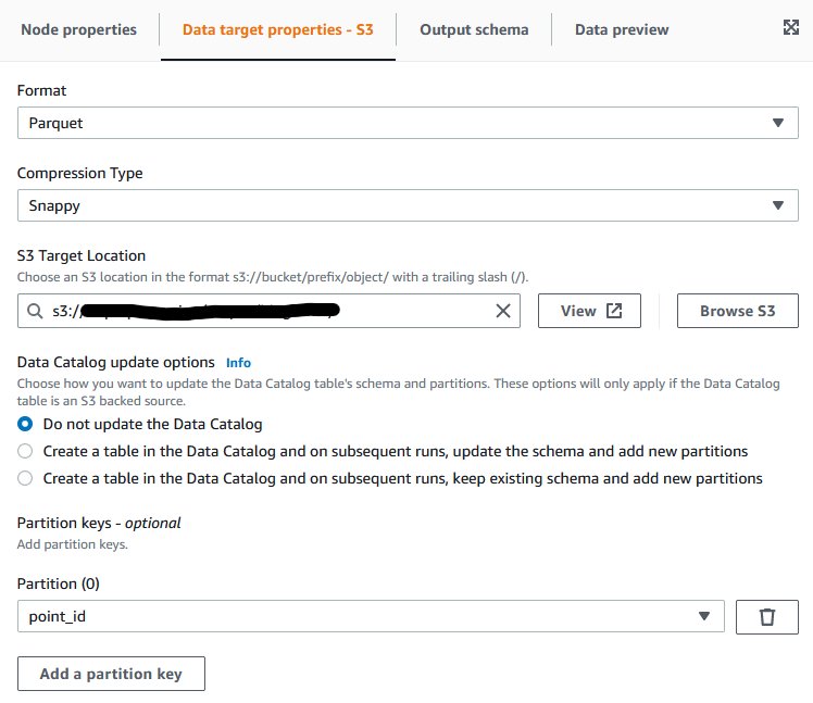
To illustrate our use case, we assume a data analyst persona who is interested in analyzing near-real-time data for sport events using the table ticket_activity. An example of this table is shown in the following screenshot.
Apache Hudi connector for AWS Glue
For this post, we use AWS Glue 4.0, which already has native support for the Hudi framework. Hudi, an open-source data lake framework, simplifies incremental data processing in data lakes built on Amazon S3. It enables capabilities including time travel queries, ACID (Atomicity, Consistency, Isolation, Durability) transactions, streaming ingestion, CDC, upserts, and deletes.
Set up resources with AWS CloudFormation
This post includes a CloudFormation template for a quick setup. You can review and customize it to suit your needs.
The CloudFormation template generates the following resources:
An RDS database instance (source).
An AWS DMS replication instance, used to replicate the data from the source table to Kinesis Data Streams.
A Kinesis data stream.
Four AWS Glue Python shell jobs:
rds-ingest-rds-setup-<CloudFormation Stack name> – creates one source table called ticket_activity on Amazon RDS.
rds-ingest-data-initial-<CloudFormation Stack name> – Sample data is automatically generated at random by the Faker library and loaded to the ticket_activity table.
rds-ingest-data-incremental-<CloudFormation Stack name> – Ingests new ticket activity data into the source table ticket_activity continuously. This job simulates customer activity.
rds-upsert-data-<CloudFormation Stack name> – Upserts specific records in the source table ticket_activity. This job simulates administrator activity.
An Amazon VPC, a public subnet, two private subnets, internet gateway, NAT gateway, and route tables.
We use private subnets for the RDS database instance and AWS DMS replication instance.
We use the NAT gateway to have reachability to pypi.org to use the MySQL connector for Python from the AWS Glue Python shell jobs. It also provides reachability to Kinesis Data Streams and an Amazon S3 API endpoint
To set up these resources, you must have the following prerequisites:
If you already deselected Use only IAM access control for new databases and Use only IAM access control for new table in new databases on the AWS Lake Formation console Settings page, you need to select these two check boxes again and save your settings. For more information, see Changing the default settings for your data lake.
The following diagram illustrates the architecture of our provisioned resources.
To launch the CloudFormation stack, complete the following steps:
Sign in to the AWS CloudFormation console.
Choose Launch Stack
Choose Next.
For S3BucketName, enter the name of your new S3 bucket.
For VPCCIDR, enter a CIDR IP address range that doesn’t conflict with your existing networks.
For PublicSubnetCIDR, enter the CIDR IP address range within the CIDR you gave for VPCCIDR.
For PrivateSubnetACIDR and PrivateSubnetBCIDR, enter the CIDR IP address range within the CIDR you gave for VPCCIDR.
For SubnetAzA and SubnetAzB, choose the subnets you want to use.
For DatabaseUserName, enter your database user name.
For DatabaseUserPassword, enter your database user password.
Choose Next.
On the next page, choose Next.
Review the details on the final page and select I acknowledge that AWS CloudFormation might create IAM resources with custom names.
Choose Create stack.
Stack creation can take about 20 minutes.
Set up an initial source table
The AWS Glue job rds-ingest-rds-setup-<CloudFormation stack name> creates a source table called event on the RDS database instance. To set up the initial source table in Amazon RDS, complete the following steps:
On the AWS Glue console, choose Jobs in the navigation pane.
Choose rds-ingest-rds-setup-<CloudFormation stack name> to open the job.
Choose Run.
Navigate to the Runs tab and wait for Run status to show as SUCCEEDED.
This job will only create the one table, ticket_activity, in the MySQL instance (DDL). See the following code:
CREATE TABLE ticket_activity (
ticketactivity_id INT NOT NULL AUTO_INCREMENT PRIMARY KEY,
sport_type VARCHAR(256) NOT NULL,
start_date DATETIME NOT NULL,
location VARCHAR(256) NOT NULL,
seat_level VARCHAR(256) NOT NULL,
seat_location VARCHAR(256) NOT NULL,
ticket_price INT NOT NULL,
customer_name VARCHAR(256) NOT NULL,
email_address VARCHAR(256) NOT NULL,
created_at DATETIME NOT NULL,
updated_at DATETIME NOT NULL )
Ingest new records
In this section, we detail the steps to ingest new records. Implement following steps to star the execution of the jobs.
Start data ingestion to Kinesis Data Streams using AWS DMS
To start data ingestion from Amazon RDS to Kinesis Data Streams, complete the following steps:
On the AWS DMS console, choose Database migration tasks in the navigation pane.
Select the task rds-to-kinesis-<CloudFormation stack name>.
On the Actions menu, choose Restart/Resume.
Wait for the status to show as Load complete and Replication ongoing.
The AWS DMS replication task ingests data from Amazon RDS to Kinesis Data Streams continuously.
Start data ingestion to Amazon S3
Next, to start data ingestion from Kinesis Data Streams to Amazon S3, complete the following steps:
On the AWS Glue console, choose Jobs in the navigation pane.
Choose streaming-cdc-kinesis2hudi-<CloudFormation stack name> to open the job.
Choose Run.
Do not stop this job; you can check the run status on the Runs tab and wait for it to show as Running.
Start the data load to the source table on Amazon RDS
To start data ingestion to the source table on Amazon RDS, complete the following steps:
On the AWS Glue console, choose Jobs in the navigation pane.
Choose rds-ingest-data-initial-<CloudFormation stack name> to open the job.
Choose Run.
Navigate to the Runs tab and wait for Run status to show as SUCCEEDED.
Validate the ingested data
After about 2 minutes from starting the job, the data should be ingested into the Amazon S3. To validate the ingested data in the Athena, complete the following steps:
On the Athena console, complete the following steps if you’re running an Athena query for the first time:
On the Settings tab, choose Manage.
Specify the stage directory and the S3 path where Athena saves the query results.
Choose Save.
On the Editor tab, run the following query against the table to check the data:
SELECT * FROM "database_<account_number>_hudi_cdc_demo"."ticket_activity" limit 10;
Note that AWS Cloud Formation will create the database with the account number as database_<your-account-number>_hudi_cdc_demo.
Update existing records
Before you update the existing records, note down the ticketactivity_id value of a record from the ticket_activity table. Run the following SQL using Athena. For this post, we use ticketactivity_id = 46 as an example:
SELECT * FROM "database_<account_number>_hudi_cdc_demo"."ticket_activity" limit 10;
To simulate a real-time use case, update the data in the source table ticket_activity on the RDS database instance to see that the updated records are replicated to Amazon S3. Complete the following steps:
On the AWS Glue console, choose Jobs in the navigation pane.
Choose rds-ingest-data-incremental-<CloudFormation stack name> to open the job.
Choose Run.
Choose the Runs tab and wait for Run status to show as SUCCEEDED.
To upsert the records in the source table, complete the following steps:
On the AWS Glue console, choose Jobs in the navigation pane.
Choose the job rds-upsert-data-<CloudFormation stack name>.
On the Job details tab, under Advanced properties, for Job parameters, update the following parameters:
For Key, enter --ticketactivity_id.
For Value, replace 1 with one of the ticket IDs you noted above (for this post, 46).
Choose Save.
Choose Run and wait for the Run status to show as SUCCEEDED.
This AWS Glue Python shell job simulates a customer activity to buy a ticket. It updates a record in the source table ticket_activity on the RDS database instance using the ticket ID passed in the job argument --ticketactivity_id. It will update ticket_price=500 and updated_at with the current timestamp.
To validate the ingested data in Amazon s3, run the same query from Athena and check the ticket_activity value you noted earlier to observe the ticket_price and updated_at fields:
SELECT * FROM "database_<account_number>_hudi_cdc_demo"."ticket_activity" where ticketactivity_id = 46 ;
Visualize the data in QuickSight
After you have the output file generated by the AWS Glue streaming job in the S3 bucket, you can use QuickSight to visualize the Hudi data files. QuickSight is a scalable, serverless, embeddable, ML-powered business intelligence (BI) service built for the cloud. QuickSight lets you easily create and publish interactive BI dashboards that include ML-powered insights. QuickSight dashboards can be accessed from any device and seamlessly embedded into your applications, portals, and websites.
Build a QuickSight dashboard
To build a QuickSight dashboard, complete the following steps:
Open the QuickSight console.
You’re presented with the QuickSight welcome page. If you haven’t signed up for QuickSight, you may have to complete the signup wizard. For more information, refer to Signing up for an Amazon QuickSight subscription.
After you have signed up, QuickSight presents a “Welcome wizard.” You can view the short tutorial, or you can close it.
On the QuickSight console, choose your user name and choose Manage QuickSight.
Choose Security & permissions, then choose Manage.
Select Amazon S3 and select the buckets that you created earlier with AWS CloudFormation.
Select Amazon Athena.
Choose Save.
If you changed your Region during the first step of this process, change it back to the Region that you used earlier during the AWS Glue jobs.
Create a dataset
Now that you have QuickSight up and running, you can create your dataset. Complete the following steps:
On the QuickSight console, choose Datasets in the navigation pane.
Choose New dataset.
Choose Athena.
For Data source name, enter a name (for example, hudi-blog).
Choose Validate.
After the validation is successful, choose Create data source.
For Database, choose database_<your-account-number>_hudi_cdc_demo.
For Tables, select ticket_activity.
Choose Select.
Choose Visualize.
Choose hour and then ticket_activity_id to get the count of ticket_activity_id by hour.
Clean up
To clean up your resources, complete the following steps:
Stop the AWS DMS replication task rds-to-kinesis-<CloudFormation stack name>.
Navigate to the RDS database and choose Modify.
Deselect Enable deletion protection, then choose Continue.
Stop the AWS Glue streaming job streaming-cdc-kinesis2redshift-<CloudFormation stack name>.
On the QuickSight dashboard, choose your user name, then choose Manage QuickSight.
Choose Account settings, then choose Delete account.
Choose Delete account to confirm.
Enter confirm and choose Delete account.
Conclusion
In this post, we demonstrated how you can stream data—not only new records, but also updated records from relational databases—to Amazon S3 using an AWS Glue streaming job to create an Apache Hudi-based near-real-time transactional data lake. With this approach, you can easily achieve upsert use cases on Amazon S3. We also showcased how to visualize the Apache Hudi table using QuickSight and Athena. As a next step, refer to the Apache Hudi performance tuning guide for a high-volume dataset. To learn more about authoring dashboards in QuickSight, check out the QuickSight Author Workshop.
About the Authors
Raj Ramasubbu is a Sr. Analytics Specialist Solutions Architect focused on big data and analytics and AI/ML with Amazon Web Services. He helps customers architect and build highly scalable, performant, and secure cloud-based solutions on AWS. Raj provided technical expertise and leadership in building data engineering, big data analytics, business intelligence, and data science solutions for over 18 years prior to joining AWS. He helped customers in various industry verticals like healthcare, medical devices, life science, retail, asset management, car insurance, residential REIT, agriculture, title insurance, supply chain, document management, and real estate.
Rahul Sonawane is a Principal Analytics Solutions Architect at AWS with AI/ML and Analytics as his area of specialty.
Sundeep Kumar is a Sr. Data Architect, Data Lake at AWS, helping customers build data lake and analytics platform and solutions. When not building and designing data lakes, Sundeep enjoys listening music and playing guitar.
Today, more than 400 organizations have signed The Climate Pledge, a commitment to reach net-zero carbon by 2040. Some of the drivers that lead to setting explicit climate goals include customer demand, current and anticipated government relations, employee demand, investor demand, and sustainability as a competitive advantage. AWS customers are increasingly interested in ways to drive sustainability actions. In this blog, we will walk through how we can apply existing enterprise data to better understand and estimate Scope 1 carbon footprint using Amazon Simple Storage Service (S3) and Amazon Athena, a serverless interactive analytics service that makes it easy to analyze data using standard SQL.
The Greenhouse Gas Protocol
The Greenhouse Gas Protocol (GHGP) provides standards for measuring and managing global warming impacts from an organization’s operations and value chain.
The greenhouse gases covered by the GHGP are the seven gases required by the UNFCCC/Kyoto Protocol (which is often called the “Kyoto Basket”). These gases are carbon dioxide (CO2), methane (CH4), nitrous oxide (N2O), the so-called F-gases (hydrofluorocarbons and perfluorocarbons), sulfur hexafluoride (SF6) nitrogen trifluoride (NF3). Each greenhouse gas is characterized by its global warming potential (GWP), which is determined by the gas’s greenhouse effect and its lifetime in the atmosphere. Since carbon dioxide (CO2) accounts for about 76 percent of total man-made greenhouse gas emissions, the global warming potential of greenhouse gases are measured relative to CO2, and are thus expressed as CO2-equivalent (CO2e).
The GHGP divides an organization’s emissions into three primary scopes:
Scope 1 – Direct greenhouse gas emissions (for example from burning fossil fuels)
Scope 2 – Indirect emissions from purchased energy (typically electricity)
Scope 3 – Indirect emissions from the value chain, including suppliers and customers
How do we estimate greenhouse gas emissions?
There are different methods to estimating GHG emissions that includes the Continuous Emissions Monitoring System (CEMS) Method, the Spend-Based Method, and the Consumption-Based Method.
Direct Measurement – CEMS Method
An organization can estimate its carbon footprint from stationary combustion sources by performing a direct measurement of carbon emissions using the CEMS method. This method requires continuously measuring the pollutants emitted in exhaust gases from each emissions source using equipment such as gas analyzers, gas samplers, gas conditioning equipment (to remove particulate matter, water vapor and other contaminants), plumbing, actuated valves, Programmable Logic Controllers (PLCs) and other controlling software and hardware. Although this approach may yield useful results, CEMS requires specific sensing equipment for each greenhouse gas to be measured, requires supporting hardware and software, and is typically more suitable for Environment Health and Safety applications of centralized emission sources. More information on CEMS is available here.
Spend-Based Method
Because the financial accounting function is mature and often already audited, many organizations choose to use financial controls as a foundation for their carbon footprint accounting. The Economic Input-Output Life Cycle Assessment (EIO LCA) method is a spend-based method that combines expenditure data with monetary-based emission factors to estimate the emissions produced. The emission factors are published by the U.S. Environment Protection Agency (EPA) and other peer-reviewed academic and government sources. With this method, you can multiply the amount of money spent on a business activity by the emission factor to produce the estimated carbon footprint of the activity.
For example, you can convert the amount your company spends on truck transport to estimated kilograms (KG) of carbon dioxide equivalent (CO₂e) emitted as shown below.
Estimated Carbon Footprint = Amount of money spent on truck transport * Emission Factor [1]
Although these computations are very easy to make from general ledgers or other financial records, they are most valuable for initial estimates or for reporting minor sources of greenhouse gases. As the only user-provided input is the amount spent on an activity, EIO LCA methods aren’t useful for modeling improved efficiency. This is because the only way to reduce EIO-calculated emissions is to reduce spending. Therefore, as a company continues to improve its carbon footprint efficiency, other methods of estimating carbon footprint are often more desirable.
Consumption-Based Method
From either Enterprise Resource Planning (ERP) systems or electronic copies of fuel bills, it’s straightforward to determine the amount of fuel an organization procures during a reporting period. Fuel-based emission factors are available from a variety of sources such as the US Environmental Protection Agency and commercially-licensed databases. Multiplying the amount of fuel procured by the emission factor yields an estimate of the CO2e emitted through combustion. This method is often used for estimating the carbon footprint of stationary emissions (for instance backup generators for data centers or fossil fuel ovens for industrial processes).
If for a particular month an enterprise consumed a known amount of motor gasoline for stationary combustion, the Scope 1 CO2e footprint of the stationary gasoline combustion can be estimated in the following manner:
Organizations may estimate their carbon emissions by using existing data found in fuel and electricity bills, ERP data, and relevant emissions factors, which are then consolidated in to a data lake. Using existing analytics tools such as Amazon Athena and Amazon QuickSight an organization can gain insight into its estimated carbon footprint.
The data architecture diagram below shows an example of how you could use AWS services to calculate and visualize an organization’s estimated carbon footprint.
Customers have the flexibility to choose the services in each stage of the data pipeline based on their use case. For example, in the data ingestion phase, depending on the existing data requirements, there are many options to ingest data into the data lake such as using the AWS Command Line Interface (CLI),AWS DataSync, or AWS Database Migration Service.
Example of calculating a Scope 1 stationary emissions footprint with AWS services
Let’s assume you burned 100 standard cubic feet (scf) of natural gas in an oven. Using the US EPA emission factors for stationary emissions we can estimate the carbon footprint associated with the burning. In this case the emission factor is 0.05449555 Kg CO2e /scf.[3]
Amazon S3 is ideal for building a data lake on AWS to store disparate data sources in a single repository, due to its virtually unlimited scalability and high durability. Athena, a serverless interactive query service, allows the analysis of data directly from Amazon S3 using standard SQL without having to load the data into Athena or run complex extract, transform, and load (ETL) processes. Amazon QuickSight supports creating visualizations of different data sources, including Amazon S3 and Athena, and the flexibility to use custom SQL to extract a subset of the data. QuickSight dashboards can provide you with insights (such as your company’s estimated carbon footprint) quickly, and also provide the ability to generate standardized reports for your business and sustainability users.
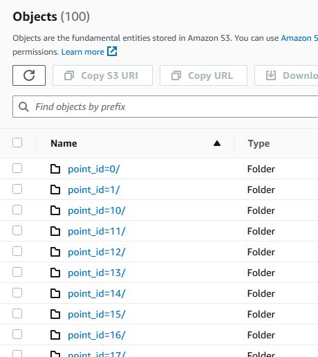
The snapshot of the S3 console shows two newly added folders that contains the files.
To create new table schemas, we start by running the following script for the gas utilization table in the Athena query editor using Hive DDL. The script defines the data format, column details, table properties, and the location of the data in S3.
After creating the table schema in Athena, we run the below query against the gas utilization table that includes details of gas bills to show the gas utilization and the associated charges, such as gas public purpose program surcharge (PPPS) and total charges after taxes for the year of 2020:
SELECT * FROM "gasutilization" where year = 2020;
We are also able to analyze the emission factor data showing the different fuel types and their corresponding CO2e emission as shown in the screenshot.
With the emission factor and the gas utilization data, we can run the following query below to get an estimated Scope 1 carbon footprint alongside other details. In this query, we joined the gas utilization table and the gas emission factor table on fuel id and multiplied the gas usage in standard cubic foot (scf) by the emission factor to get the estimated CO2e impact. We also selected the month, year, total charge, and gas usage measured in therms and scf, as these are often attributes that are of interest for customers.
SELECT "gasutilization"."usage_scf" * "gas_emission_factor"."emission_factor"
AS "estimated_CO2e_impact",
"gasutilization"."month",
"gasutilization"."year",
"gasutilization"."totalcharge",
"gasutilization"."usage_therms",
"gasutilization"."usage_scf"
FROM "gasutilization"
JOIN "gas_emission_factor"
on "gasutilization"."fuel_id"="gas_emission_factor"."fuel_id";
Lastly, Amazon QuickSight allows visualization of different data sources, including Amazon S3 and Athena, and the flexibility to use custom SQL to get a subset of the data. The following is an example of a QuickSight dashboard showing the gas utilization, gas charges, and estimated carbon footprint across different years.
We have just estimated the Scope 1 carbon footprint for one source of stationary combustion. If we were to do the same process for all sources of stationary and mobile emissions (with different emissions factors) and add the results together, we could roll up an accurate estimate of our Scope 1 carbon emissions for the entire business by only utilizing native AWS services and our own data. A similar process will yield an estimate of Scope 2 emissions, with grid carbon intensity in the place of Scope 1 emission factors.
Summary
This blog discusses how organizations can use existing data in disparate sources to build a data architecture to gain better visibility into Scope 1 greenhouse gas emissions. With Athena, S3, and QuickSight, organizations can now estimate their stationary emissions carbon footprint in a repeatable way by applying the consumption-based method to convert fuel utilization into an estimated carbon footprint.
If you are interested in information on estimating your organization’s carbon footprint with AWS, please reach out to your AWS account team and check out AWS Sustainability Solutions.
References
An example from page four of Amazon’s Carbon Methodology document illustrates this concept. Amount spent on truck transport: $100,000 EPA Emission Factor: 1.556 KG CO2e /dollar of truck transport Estimated CO₂e emission: $100,000 * 1.556 KG CO₂e/dollar of truck transport = 155,600 KG of CO2e ↑
For example, Gasoline consumed: 1,000 US Gallons EPA Emission Factor: 8.81 Kg of CO2e /gallon of gasoline combusted Estimated CO2e emission = 1,000 US Gallons * 8.81 Kg of CO2e per gallon of gasoline consumed= 8,810 Kg of CO2e. EPA Emissions Factor for stationary emissions of motor gasoline is 8.78 kg CO2 plus .38 grams of CH4, plus .08 g of N2O. Combining these emission factors using 100-year global warming potential for each gas (CH4:25 and N2O:298) gives us Combined Emission Factor = 8.78 kg + 25*.00038 kg + 298 *.00008 kg = 8.81 kg of CO2e per gallon.↑
The Emission factor per scf is 0.05444 kg of CO2 plus 0.00103 g of CH4 plus 0.0001 g of N2O. To get this in terms of CO2e we need to multiply the emission factor of the other two gases by their global warming potentials (GWP). The 100-year GWP for CH4 and N2O are 25 and 298 respectively. Emission factors and GWPs come from the US EPA website. ↑
About the Authors
Thomas Burns,SCR, CISSP is a Principal Sustainability Strategist and Principal Solutions Architect at Amazon Web Services. Thomas supports manufacturing and industrial customers world-wide. Thomas’s focus is using the cloud to help companies reduce their environmental impact both inside and outside of IT.
Aileen Zheng is a Solutions Architect supporting US Federal Civilian Sciences customers at Amazon Web Services (AWS). She partners with customers to provide technical guidance on enterprise cloud adoption and strategy and helps with building well-architected solutions. She is also very passionate about data analytics and machine learning. In her free time, you’ll find Aileen doing pilates, taking her dog Mumu out for a hike, or hunting down another good spot for food! You’ll also see her contributing to projects to support diversity and women in technology.
Amazon Kinesis Data Streams is a serverless data streaming service that makes it easy to capture, process, and store streaming data at any scale. As customers collect and stream more types of data, they have asked for simpler, elastic data streams that can handle variable and unpredictable data traffic. In November 2021, Amazon Web Services launched the on-demand capacity mode for Kinesis Data Streams, which is capable of serving gigabytes of write and read throughput per minute and helps reduce the operational pain point of manually updating data stream capacity. You can create a new on-demand data stream or convert an existing data stream to on-demand mode with a single click and never have to provision and manage servers, storage, or throughput. By default, on-demand capacity mode can automatically scale up to 200 MB/s of write throughput.
We were encouraged by customers’ adoption of on-demand capacity mode, but as customers scaled their workloads, some ran into the 200 MB/s data ingestion limit and asked for a solution. The team worked backward from customer feedback to raise that limit. As of March 2023, Kinesis Data Streams supports an increased on-demand write throughput limit to 1 GB/s, a five-times increase from the current limit of 200 MB/s. It’s like having a truly serverless and elastic data streaming service that works for all your use cases. If you require an increase in capacity, you can contact AWS Support to enable on-demand streams to scale up to 1 GB/s write throughput for each requested account. You pay for throughput consumed rather than for provisioned resources, making it easier to balance costs and performance. Overall, if your data volume can spike unpredictably or you don’t want to manage the number of shards, use on-demand streams.
In this post, we explore how to use Kinesis Data Streams on-demand scaling and best practices to build an efficient data-streaming solution. We discuss different scenarios to avoid write throughput exceptions and scale ingest capacity of Kinesis Data Streams to 1 GB/s in on-demand capacity mode.
Kinesis Data Streams on-demand scaling
A shard serves as a base throughput unit of Kinesis Data Streams. A shard supports 1 MB/s and 1,000 records/s for writes and 2 MB/s for reads. The shard limits ensure predictable performance, making it easy to design and operate a highly reliable data streaming workflow. In on-demand capacity mode, scaling happens at the individual shard level. When the average ingest shard utilization reaches 50% (0.5 MB/s or 500 records/s) in 1 minute, then a shard is split into two shards. If you use random values as a partition key, all shards of the stream will have even traffic, and they will be scaled at the same time. If you use a business-specific key as a partition key, the shards will have uneven traffic. In that scenario, only the shards exceeding an average of 50% utilization will be scaled. Depending upon the number of shards being scaled, it will take up to 15 minutes to split the shards.
When we create a new Kinesis data stream in on-demand capacity mode, by default, Kinesis Data Streams provisions four shards, which provides 4 MB/s write and 8 MB/s read throughput. As the workload ramps up, Kinesis Data Streams increases the number of shards in the stream by monitoring ingest throughput at the shard level. The 4 MB/s default ingest throughput and scaling at shard level in on-demand capacity mode works for most use cases. However, in some specific scenarios, producers may face WriteThroughputExceeded and Rate Exceeded errors, even in on-demand capacity mode. We discuss a few of these scenarios in the following sections and strategies to avoid these errors.
You can create and save record templates and easily send data to Kinesis Data Streams using the Amazon Kinesis Data Generator (KDG) to test the streaming data solution. Alternatively, you can also use the modern load testing framework Locust to run large-scale Kinesis Data Streams load testing. For this post, we use the Locust tool to produce and ingest messages in Kinesis Data Streams for our different use cases.
Scenario 1: A baseline ingest throughput greater than 4 MB/s is needed
To simulate this scenario, run the following AWS Command Line Interface (AWS CLI) command to create the kds-od-default-shards data stream in on-demand capacity mode:
You can observe that the OpenShardCount value is 4, which means the kds-od-default-shards data stream has an ingest capacity of 4 MB/s.
Next, we use the Locust tool to set the baseline to approximately 25 MB/s records. As displayed in the following Amazon CloudWatch metrics graph, records are getting throttled for the first couple of minutes. Then the kds-od-default-shards data stream scales the number of shards to support 25 MB/s ingest throughput, and records stop getting throttled. You can also rerun the describe-stream-summary AWS CLI command to check the increased number of shards in the data stream.
In a scenario where we know our ingest throughput baseline (25 MB/s) ahead of the time and we don’t want to observe any write throttles, we can create a stream in provisioned mode by specifying the number of shards (30), as shown in the following AWS CLI command (make sure to delete kds-od-default-shards manually from the Kinesis Data Streams console before running the following command):
Next, we send 25 MB/s records to the kds-od-default-shards data stream. As displayed in the following CloudWatch metrics graph, we can observe no write throttles, and the kds-od-default-shards data stream scales the number of shards to handle the increase in ingest volume.
After we send 25 MB/s traffic to the data stream for some time, we can run following AWS CLI command to see that the OpenShardCount value is increased to more than 30 now:
As mentioned earlier, by default, the kds-od-significant-spike data stream will have four shards initially because this stream is created in on-demand mode. When the data stream is active, we send 4 MB/s ingest throughput initially and grow the ingest throughput by 30–50% every 5–10 minutes. As displayed in the following CloudWatch metrics graph, the kds-od-significant-spike data stream scales the number of shards to handle the increase in ingest volume.
After approximately 15 minutes, run the following AWS CLI command to find the OpenShardCount value (x) of the kds-od-significant-spike data stream. Then send (x * 2) MB/s ingest throughput in the data stream for 2–3 minutes and reduced ingest throughput to the prior level:
As displayed in the following CloudWatch metrics graph, the records are getting throttled for a few minutes, and then the throttling goes away.
Typically, we face a significant spike scenario when running planned events, such as shopping holidays and product launches. To handle such scenarios, we can proactively change capacity mode from on-demand to provisioned. We can configure the number of shards and pick the ingest capacity we anticipate. After we successfully scale the number of shards to our desired peak capacity in provisioned capacity mode, we can change the capacity mode back to on-demand mode.
Scenario 3: A single partition key starts pushing more than 1 MB/s
Partition keys are used to segregate and route records to different shards of a stream. A partition key is specified by the data producer while adding data to the data stream. For example, let’s assume we have a stream with two shards (shard 1 and shard 2). We can configure the data producer to use two partition keys (key A and key B) so that all records with key A are added to shard 1 and all records with key B are added to shard 2. Choosing a partition key is a very important decision, and we should carefully pick the partition key to ensure equal distribution of records across all the shards of the stream. Messages tied to a single partition key A will be sent to a single shard (shard 1), and at any given instance, messages tied to a single partition key A cannot be distributed across different shards. As mentioned earlier, by default, one shard supports 1 MB/s and 1,000 records/s for writes, and we may end up with an edge case scenario where we are trying to push more than 1 MB/s for a specific partition key. In this scenario, producers will continue to experience throttles and keep retrying indefinitely.
To simulate the scenario, run the following AWS CLI command to create the kds-od-partition-key-throttle data stream in on-demand capacity mode:
As mentioned earlier, by default, the data stream will have four shards initially because this stream is created in on-demand mode. When the data stream is active, we send 1.5 MB/s ingest throughput continuously for the specific partition key A. As displayed in the following CloudWatch metrics graph, we can observe that throttling continues from a single shard even if we are sending 1.5 MB/s ingest throughput, and the kds-od-partition-key-throttle data stream has an overall ingest capacity of 4 MB/s.
To avoid this scenario, we should carefully pick our partition key and ensure that this specific partition key won’t be continuously sending more than 1 MB/s ingest throughput in the data stream.
Scale the ingest capacity of Kinesis Data Streams to 1 GB/s in on-demand capacity mode
To test, we start with approximately 100 MB/s baseline ingest throughput to Kinesis Data Streams in on-demand capacity mode, then we increase ingest throughput rate by 30–50% every 5–10 minutes using Locust load testing tool.
To set up the scenario, first create the kds-od-1gb-stream data stream in provisioned capacity mode and provide a value of 120 for the provisioned shards field:
When the kds-od-1gb-stream data stream is active, switch its capacity mode to on-demand, as shown in the following code. When we change capacity mode from provisioned to on-demand, the shard count (120) remains the same for the data stream even in on-demand capacity mode.
When the kds-od-1gb-stream data stream is in on-demand mode, start the experiment. We send approximately 100 MB/s baseline ingest throughput using the Locust tool and increase 30–50% ingest throughput every 5–10 minutes. As displayed in the following CloudWatch metrics graph, the kds-od-1gb-stream data stream seamlessly scaled to 1 GB/s in on-demand capacity mode. We can also observe that the producers didn’t encounter any write throttles while the data stream was scaling in on-demand capacity mode.
Clean up
To avoid ongoing costs, delete all the data streams that you created as part of this post using the Kinesis Data Streams console.
Conclusion
This post demonstrated the on-demand scaling policy of Kinesis Data Streams with a few scenarios using best practices and showed how to scale ingest capacity to 1 GB/s in on-demand capacity mode. You can have an on-demand write throughput limit that is five times larger than the previous limit of 200 MB/s. Choose on-demand mode if you create new data streams with unknown workloads, have unpredictable application traffic, or prefer not to manage capacity. You can switch between on-demand and provisioned capacity modes two times per 24-hour rolling period. Please leave any feedback in the comments section.
About the Authors
Nihar Sheth is a Senior Product Manager on the Amazon Kinesis Data Streams team at Amazon Web Services. He is passionate about developing intuitive product experiences that solve complex customer problems and enable customers to achieve their business goals.
Pratik Patel is Sr. Technical Account Manager and streaming analytics specialist. He works with AWS customers and provides ongoing support and technical guidance to help plan and build solutions using best practices and proactively keep customers’ AWS environments operationally healthy.
Nisha Dekhtawala is a Partner Solutions Architect and data analytics specialist. She works with global consulting partners as their trusted advisor, providing technical guidance and support in building Well-Architected innovative industry solutions.
Data has become an integral part of most companies, and the complexity of data processing is increasing rapidly with the exponential growth in the amount and variety of data. Data engineering teams are faced with the following challenges:
Manipulating data to make it consumable by business users
Building and improving extract, transform, and load (ETL) pipelines
Scaling their ETL infrastructure
Many customers migrating data to the cloud are looking for ways to modernize by using native AWS services to further scale and efficiently handle ETL tasks. In the early stages of their cloud journey, customers may need guidance on modernizing their ETL workload with minimal effort and time. Customers often use many SQL scripts to select and transform the data in relational databases hosted either in an on-premises environment or on AWS and use custom workflows to manage their ETL.
AWS Glue is a serverless data integration and ETL service with the ability to scale on demand. In this post, we show how you can migrate your existing SQL-based ETL workload to AWS Glue using Spark SQL, which minimizes the refactoring effort.
Solution overview
The following diagram describes the high-level architecture for our solution. This solution decouples the ETL and analytics workloads from our transactional data source Amazon Aurora, and uses Amazon Redshift as the data warehouse solution to build a data mart. In this solution, we employ AWS Database Migration Service (AWS DMS) for both full load and continuous replication of changes from Aurora. AWS DMS enables us to capture deltas, including deletes from the source database, through the use of Change Data Capture (CDC) configuration. CDC in DMS enables us to capture deltas without writing code and without missing any changes, which is critical for the integrity of the data. Please refer CDC support in DMS to extend the solutions for ongoing CDC.
AWS DMS replicates data from Aurora and migrates to the target destination Amazon Simple Storage Service (Amazon S3) bucket.
AWS Glue crawlers automatically infer schema information of the S3 data and integrate into the AWS Glue Data Catalog.
AWS Glue jobs run ETL code to transform and load the data to Amazon Redshift.
For this post, we use the TPCH dataset for sample transactional data. The components of TPCH consist of eight tables. The relationships between columns in these tables are illustrated in the following diagram.
We use Amazon Redshift as the data warehouse to implement the data mart solution. The data mart fact and dimension tables are created in the Amazon Redshift database. The following diagram illustrates the relationships between the fact (ORDER) and dimension tables (DATE, PARTS, and REGION).
Set up the environment
To get started, we set up the environment using AWS CloudFormation. Complete the following steps:
Choose Launch Stack and open the page on a new tab:
Choose Next.
For Stack name, enter a name.
In the Parameters section, enter the required parameters.
Choose Next.
On the Configure stack options page, leave all values as default and choose Next.
On the Review stack page, select the check boxes to acknowledge the creation of IAM resources.
Choose Submit.
Wait for the stack creation to complete. You can examine various events from the stack creation process on the Events tab. When the stack creation is complete, you will see the status CREATE_COMPLETE. The stack takes approximately 25–30 minutes to complete.
This template configures the following resources:
The Aurora MySQL instance sales-db.
The AWS DMS task dmsreplicationtask-* for full load of data and replicating changes from Aurora (source) to Amazon S3 (destination).
AWS Glue jobs insert_region_dim_tbl, insert_parts_dim_tbl, and insert_date_dim_tbl. We use these jobs for the use cases covered in this post. We create the insert_orders_fact_tbl AWS Glue job manually using AWS Glue Visual Studio.
The Redshift cluster blog_cluster with database sales and fact and dimension tables.
An S3 bucket to store the output of the AWS Glue job runs.
IAM roles and policies with appropriate permissions.
Replicate data from Aurora to Amazon S3
Now let’s look at the steps to replicate data from Aurora to Amazon S3 using AWS DMS:
On the AWS DMS console, choose Database migration tasks in the navigation pane.
Select the task dmsreplicationtask-* and on the Action menu, choose Restart/Resume.
This will start the replication task to replicate the data from Aurora to the S3 bucket. Wait for the task status to change to Full Load Complete. The data from the Aurora tables is now copied to the S3 bucket under a new folder, sales.
Create AWS Glue Data Catalog tables
Now let’s create AWS Glue Data Catalog tables for the S3 data and Amazon Redshift tables:
On the AWS Glue console, under Data Catalog in the navigation pane, choose Connections.
Select RedshiftConnection and on the Actions menu, choose Edit.
Choose Save changes.
Select the connection again and on the Actions menu, choose Test connection.
For IAM role¸ choose GlueBlogRole.
Choose Confirm.
Testing the connection can take approximately 1 minute. You will see the message “Successfully connected to the data store with connection blog-redshift-connection.” If you have trouble connecting successfully, refer to Troubleshooting connection issues in AWS Glue.
Under Data Catalog in the navigation pane, choose Crawlers.
Select s3_crawler and choose Run.
This will generate eight tables in the AWS Glue Data Catalog. To view the tables created, in the navigation pane, choose Databases under Data Catalog, then choose salesdb.
Repeat the steps to run redshift_crawler and generate four additional tables.
Now let’s look at how the SQL statements are used to create ETL jobs using AWS Glue. AWS Glue runs your ETL jobs in an Apache Spark serverless environment. AWS Glue runs these jobs on virtual resources that it provisions and manages in its own service account. AWS Glue Studio is a graphical interface that makes it simple to create, run, and monitor ETL jobs in AWS Glue. You can use AWS Glue Studio to create jobs that extract structured or semi-structured data from a data source, perform a transformation of that data, and save the result set in a data target.
Let’s go through the steps of creating an AWS Glue job for loading the orders fact table using AWS Glue Studio.
On the AWS Glue console, choose Jobs in the navigation pane.
Choose Create job.
Select Visual with a blank canvas, then choose Create.
Navigate to the Job details tab.
For Name, enter insert_orders_fact_tbl.
For IAM Role, choose GlueBlogRole.
For Job bookmark, choose Enable.
Leave all other parameters as default and choose Save.
Navigate to the Visual tab.
Choose the plus sign.
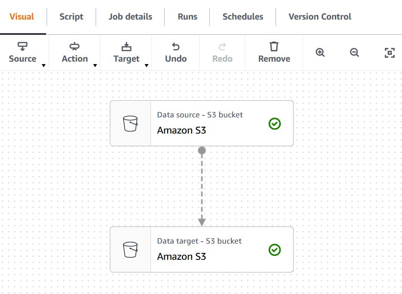
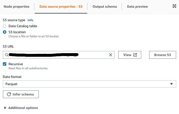
Under Add nodes, enter Glue in the search bar and choose AWS Glue Data Catalog(Source) to add the Data Catalog as the source.
In the right pane, on the Data source properties – Data Catalog tab, choose salesdb for Database and customer for Table.
On the Node properties tab, for Name, enter Customers.
Repeat these steps for the Orders and LineItem tables.
This concludes creating data sources on the AWS Glue job canvas. Next, we add transformations by combining data from these different tables.
Transform the data
Complete the following steps to add data transformations:
On the AWS Glue job canvas, choose the plus sign.
Under Transforms, choose SQL Query.
On the Transform tab, for Node parents, select all the three data sources.
On the Transform tab, under SQL query, enter the following query:
SELECT orders.o_orderkey        AS ORDERKEY,
orders.o_orderdate       AS ORDERDATE,
lineitem.l_linenumber    AS LINENUMBER,
lineitem.l_partkey       AS PARTKEY,
lineitem.l_receiptdate   AS RECEIPTDATE,
lineitem.l_quantity      AS QUANTITY,
lineitem.l_extendedprice AS EXTENDEDPRICE,
orders.o_custkey         AS CUSTKEY,
customer.c_nationkey     AS NATIONKEY,
CURRENT_TIMESTAMP        AS UPDATEDATE
FROM   orders orders,
lineitem lineitem,
customer customer
WHERE  orders.o_orderkey = lineitem.l_orderkey
AND orders.o_custkey = customer.c_custkey
Update the SQL aliases values as shown in the following screenshot.
On the Data preview tab, choose Start data preview session.
When prompted, choose GlueBlogRole for IAM role and choose Confirm.
The data preview process will take a minute to complete.
On the Output schema tab, choose Use data preview schema.
You will see the output schema similar to the following screenshot.
Now that we have previewed the data, we change a few data types.
On the AWS Glue job canvas, choose the plus sign.
Under Transforms, choose Change Schema.
Select the node.
On the Transform tab, update the Data type values as shown in the following screenshot.
Now let’s add the target node.
Choose the Change Schema node and choose the plus sign.
In the search bar, enter target.
Choose Amazon Redshift as the target.
Choose the Amazon Redshift node, and on the Data target properties – Amazon Redshift tab, for Redshift access type, select Direct data connection.
Choose RedshiftConnection for Redshift Connection, public for Schema, and order_table for Table.
Select Merge data into target table under Handling of data and target table.
Choose orderkey for Matching keys.
Choose Save.
AWS Glue Studio automatically generates the Spark code for you. You can view it on the Script tab. If you would like to do any out-of-the-box transformations, you can modify the Spark code. The AWS Glue job uses the Apache SparkSQL query for SQL query transformation. To find the available SparkSQL transformations, refer to the Spark SQL documentation.
Choose Run to run the job.
As part of the CloudFormation stack, three other jobs are created to load the dimension tables.
Navigate back to the Jobs page on the AWS Glue console, select the job insert_parts_dim_tbl, and choose Run.
This job uses the following SQL to populate the parts dimension table:
SELECT part.p_partkey,
part.p_type,
part.p_brand
FROM   part part
Select the job insert_region_dim_tbl and choose Run.
This job uses the following SQL to populate the region dimension table:
SELECT nation.n_nationkey,
nation.n_name,
region.r_name
FROM   nation,
region
WHERE  nation.n_regionkey = region.r_regionkey
Select the job insert_date_dim_tbl and choose Run.
This job uses the following SQL to populate the date dimension table:
SELECT DISTINCT( l_receiptdate )        AS DATEKEY,
Dayofweek(l_receiptdate) AS DAYOFWEEK,
Month(l_receiptdate)     AS MONTH,
Year(l_receiptdate)      AS YEAR,
Day(l_receiptdate)       AS DATE
FROM   lineitem lineitem
You can view the status of the running jobs by navigating to the Job run monitoring section on the Jobs page. Wait for all the jobs to complete. These jobs will load the data into the facts and dimension tables in Amazon Redshift.
To help optimize the resources and cost, you can use the AWS Glue Auto Scaling feature.
Verify the Amazon Redshift data load
To verify the data load, complete the following steps:
On the Amazon Redshift console, select the cluster blog-cluster and on the Query Data menu, choose Query in query editor 2.
For Authentication, select Temporary credentials.
For Database, enter sales.
For User name, enter admin.
Choose Save.
Run the following commands in the query editor to verify that the data is loaded into the Amazon Redshift tables:
SELECT *
FROM   sales.PUBLIC.order_table;

SELECT *
FROM   sales.PUBLIC.date_table;

SELECT *
FROM   sales.PUBLIC.parts_table;

SELECT *
FROM   sales.PUBLIC.region_table;
The following screenshot shows the results from one of the SELECT queries.
Now for the CDC, update the quantity of a line item for order number 1 in Aurora database using the below query. (To connect to your Aurora cluster use Cloud9 or any SQL client tools like MySQL command-line client).
UPDATE lineitem SET l_quantity = 100 WHERE l_orderkey = 1 AND l_linenumber = 4;
DMS will replicate the changes into the S3 bucket as shown in the below screenshot.
Re-running the Glue job insert_orders_fact_tbl will update the changes to the ORDER fact table as shown in the below screenshot
Clean up
To avoid incurring future charges, delete the resources created for the solution:
On the Amazon S3 console, select the S3 bucket created as part of the CloudFormation stack, then choose Empty.
On the AWS CloudFormation console, select the stack that you created initially and choose Delete to delete all the resources created by the stack.
Conclusion
In this post, we showed how you can migrate existing SQL-based ETL to an AWS serverless ETL infrastructure using AWS Glue jobs. We used AWS DMS to migrate data from Aurora to an S3 bucket, then SQL-based AWS Glue jobs to move the data to fact and dimension tables in Amazon Redshift.
This solution demonstrates a one-time data load from Aurora to Amazon Redshift using AWS Glue jobs. You can extend this solution for moving the data on a scheduled basis by orchestrating and scheduling jobs using AWS Glue workflows. To learn more about the capabilities of AWS Glue, refer to AWS Glue.
About the Authors
Mitesh Patel is a Principal Solutions Architect at AWS with specialization in data analytics and machine learning. He is passionate about helping customers building scalable, secure and cost effective cloud native solutions in AWS to drive the business growth. He lives in DC Metro area with his wife and two kids.
Sumitha AP is a Sr. Solutions Architect at AWS. She works with customers and help them attain their business objectives by designing secure, scalable, reliable, and cost-effective solutions in the AWS Cloud. She has a focus on data and analytics and provides guidance on building analytics solutions on AWS.
Deepti Venuturumilli is a Sr. Solutions Architect in AWS. She works with commercial segment customers and AWS partners to accelerate customers’ business outcomes by providing expertise in AWS services and modernize their workloads. She focuses on data analytics workloads and setting up modern data strategy on AWS.
Deepthi Paruchuri is an AWS Solutions Architect based in NYC. She works closely with customers to build cloud adoption strategy and solve their business needs by designing secure, scalable, and cost-effective solutions in the AWS cloud.
Amazon CodeCatalyst is an integrated service for software development teams adopting continuous integration and deployment practices into their software development process. CodeCatalyst puts the tools you need all in one place. You can plan work, collaborate on code, and build, test, and deploy applications by leveraging CodeCatalyst Workflows.
The post walks through how to develop, deploy and test a HTTP RESTful API to Azure Functions using Amazon CodeCatalyst. The solution covers the following steps:
Set up CodeCatalyst development environment and develop your application using the Serverless Framework.
Build a CodeCatalyst workflow to test and then deploy to Azure Functions using GitHub Actions in Amazon CodeCatalyst.
An Amazon CodeCatalyst workflow is an automated procedure that describes how to build, test, and deploy your code as part of a continuous integration and continuous delivery (CI/CD) system. You can use GitHub Actions alongside native CodeCatalyst actions in a CodeCatalyst workflow.
Access to an Azure and credentials for a service principal that has permissions to create and manage Azure Functions.
Walkthrough
In this post, we will create a hello world RESTful API using the Serverless Framework. As we progress through the solution, we will focus on building a CodeCatalyst workflow that deploys and tests the functionality of the application. At the end of the post, the workflow will look similar to the one shown in Figure 2.
Figure 2 – CodeCatalyst CI/CD workflow
Environment Setup
Before we start developing the application, we need to setup a CodeCatalyst project and then link a code repository to the project. The code repository can be CodeCatalyst Repo or GitHub. In this scenario, we’ve used GitHub repository. By the time we develop the solution, the repository should look as shown below.
Figure 3 – Files in GitHub repository
In Amazon CodeCatalyst, there’s an option to create Dev Environments, which can used to work on the code stored in the source repositories of a project. In the post, we create a Dev Environment, and associate it with the source repository created above and work off it. But you may choose not to use a Dev Environment, and can run the following commands, and commit to the repository. The /projects directory of a Dev Environment stores the files that are pulled from the source repository. In the dev environment, install the Serverless Framework using this command:
npm install -g serverless
and then initialize a serverless project in the source repository folder:
We can push the code to the CodeCatalyst project using git. Now, that we have the code in CodeCatalyst, we can turn our focus to building the workflow using the CodeCatalyst console.
CI/CD Setup in CodeCatalyst
Configure access to the Azure Environment
We’ll use the GitHub action for Serverless to create and manage Azure Function. For the action to be able to access the Azure environment, it requires credentials associated with a Service Principal passed to the action as environment variables.
Service Principals in Azure are identified by the CLIENT_ID, CLIENT_SECRET, SUBSCRIPTION_ID, and TENANT_ID properties. Storing these values in plaintext anywhere in your repository should be avoided because anyone with access to the repository which contains the secret can see them. Similarly, these values shouldn’t be used directly in any workflow definitions because they will be visible as files in your repository. With CodeCatalyst, we can protect these values by storing them as secrets within the project, and then reference the secret in the CI\CD workflow.
We can create a secret by choosing Secrets (1) under CI\CD and then selecting ‘Create Secret’ (2) as shown in Figure 4. Now, we can key in the secret name and value of each of the identifiers described above.
Figure 4 – CodeCatalyst Secrets
Building the workflow
To create a new workflow, select CI/CD from navigation on the left and then select Workflows (1). Then, select Create workflow (2), leave the default options, and select Create (3) as shown in Figure 5.
Figure 5 – Create CI/CD workflow
If the workflow editor opens in YAML mode, select Visual to open the visual designer. Now, we can start adding actions to the workflow.
Configure the Deploy action
We’ll begin by adding a GitHub action for deploying to Azure. Select “+ Actions” to open the actions list and choose GitHub from the dropdown menu. Find the Build action and click “+” to add a new GitHub action to the workflow.
Next, configure the GitHub action from the configurations tab by adding the following snippet to the GitHub Actions YAML property:
The above workflow configuration makes use of Serverless GitHub Action that wraps the Serverless Framework to run serverless commands. The action is configured to package and deploy the source code to Azure Functions using the serverless deploy command.
Please note how we were able to pass the secrets to GitHub action by referencing the secret identifiers in the above configuration.
Configure the Test action
Similar to the previous step, we add another GitHub action which will use the serverless framework’s serverless invoke command to test the API deployed on to Azure Functions.
The workflow is now ready and can be validated by choosing ‘Validate’ and then saved to the repository by choosing ‘Commit’. The workflow should automatically kick-off after commit and the application is automatically deployed to Azure Functions.
The functionality of the API can now be verified from the logs of the test action of the workflow as shown in Figure 6.
Figure 6 – CI/CD workflow Test action
Cleanup
If you have been following along with this workflow, you should delete the resources you deployed so you do not continue to incur charges. First, delete the Azure Function App (usually prefixed ‘sls’) using the Azure console. Second, delete the project from CodeCatalyst by navigating to Project settings and choosing Delete project. There’s no cost associated with the CodeCatalyst project and you can continue using it.
Conclusion
In summary, this post highlighted how Amazon CodeCatalyst can help organizations deploy cloud-native, serverless workload into multi-cloud environment. The post also walked through the solution detailing the process of setting up Amazon CodeCatalyst to deploy a serverless application to Azure Functions by leveraging GitHub Actions. Though we showed an application deployment to Azure Functions, you can follow a similar process and leverage CodeCatalyst to deploy any type of application to almost any cloud platform. Learn more and get started with your Amazon CodeCatalyst journey!
We would love to hear your thoughts, and experiences, on deploying serverless applications to multiple cloud platforms. Reach out to us if you’ve any questions, or provide your feedback in the comments section.
In the previous post of this blog series, we saw how organizations can deploy workloads to virtual machines (VMs) in a hybrid and multicloud environment. This post shows how organizations can address the requirement of deploying containers, and containerized applications to hybrid and multicloud platforms using Amazon CodeCatalyst. CodeCatalyst is an integrated DevOps service which enables development teams to collaborate on code, and build, test, and deploy applications with continuous integration and continuous delivery (CI/CD) tools.
One prominent scenario where multicloud container deployment is useful is when organizations want to leverage AWS’ broadest and deepest set of Artificial Intelligence (AI) and Machine Learning (ML) capabilities by developing and training AI/ML models in AWS using Amazon SageMaker, and deploying the model package to a Kubernetes platform on other cloud platforms, such as Azure Kubernetes Service (AKS) for inference. As shown in this workshop for operationalizing the machine learning pipeline, we can train an AI/ML model, push it to Amazon Elastic Container Registry (ECR) as an image, and later deploy the model as a container application.
Scenario description
The solution described in the post covers the following steps:
Setup Amazon CodeCatalyst environment.
Create a Dockerfile along with a manifest for the application, and a repository in Amazon ECR.
Create an Azure service principal which has permissions to deploy resources to Azure Kubernetes Service (AKS), and store the credentials securely in Amazon CodeCatalyst secret.
Create a CodeCatalyst workflow to build, test, and deploy the containerized application to AKS cluster using Github Actions.
The architecture diagram for the scenario is shown in Figure 1.
Figure 1 – Solution Architecture
Solution Walkthrough
This section shows how to set up the environment, and deploy a HTML application to an AKS cluster.
Setup Amazon ECR and GitHub code repository
Create a new Amazon ECR and a code repository. In this case we’re using GitHub as the repository but you can create a source repository in CodeCatalyst or you can choose to link an existing source repository hosted by another service if that service is supported by an installed extension. Then follow the application and Docker image creation steps outlined in Step 1 in the environment creation process in exposing Multiple Applications on Amazon EKS. Create a file named manifest.yaml as shown, and map the “image” parameter to the URL of the Amazon ECR repository created above.
Push the files to Github code repository. The multicloud-container-app github repository should look similar to Figure 2 below
Figure 2 – Files in Github repository
Configure Azure Kubernetes Service (AKS) cluster to pull private images from ECR repository
Pull the docker images from a private ECR repository to your AKS cluster by running the following command. This setup is required during the azure/k8s-deploy Github Actions in the CI/CD workflow. Authenticate Docker to an Amazon ECR registry with get-login-password by using aws ecr get-login-password. Run the following command in a shell where AWS CLI is configured, and is used to connect to the AKS cluster. This creates a secret called ecrsecret, which is used to pull an image from the private ECR repository.
A CodeCatalyst environment connected to the AWS account, where the ECR repository is configured.
Configure access to the AKS cluster
In this solution, we use three GitHub Actions – azure/login, azure/aks-set-context and azure/k8s-deploy – to login, set the AKS cluster, and deploy the manifest file to the AKS cluster respectively. For the Github Actions to access the Azure environment, they require credentials associated with an Azure Service Principal.
Service Principals in Azure are identified by the CLIENT_ID, CLIENT_SECRET, SUBSCRIPTION_ID, and TENANT_ID properties. Create the Service principal by running the following command in the azure cloud shell:
az ad sp create-for-rbac \
    --name "ghActionHTMLapplication" \
    --scope /subscriptions/<SUBSCRIPTION_ID>/resourceGroups/<RESOURCE_GROUP> \
    --role Contributor \
    --sdk-auth
The command generates a JSON output (shown in Figure 3), which is stored in CodeCatalyst secret called AZURE_CREDENTIALS. This credential is used by azure/login Github Actions.
Figure 3 – JSON output
Configure secrets inside CodeCatalyst Project
Create three secrets CLUSTER_NAME (Name of AKS cluster), RESOURCE_GROUP(Name of Azure resource group) and AZURE_CREDENTIALS(described in the previous step) as described in the working with secret document. The secrets are shown in Figure 4.
Figure 4 – CodeCatalyst Secrets
CodeCatalyst CI/CD Workflow
To create a new CodeCatalyst workflow, select CI/CD from the navigation on the left and select Workflows (1). Then, select Create workflow (2), leave the default options, and select Create (3) as shown in Figure 5.
Figure 5 – Create CodeCatalyst CI/CD workflow
Add “Push to Amazon ECR” Action
Add the Push to Amazon ECR action, and configure the environment where you created the ECR repository as shown in Figure 6. Refer to adding an action to learn how to add CodeCatalyst action.
Figure 6 – Create ‘Push to ECR’ Action
Select the Configuration tab and specify the configurations as shown in Figure7.
3. The workflow is now ready and can be validated by choosing ‘Validate’ and then saved to the repository by choosing ‘Commit’. We have implemented an automated CI/CD workflow that builds the container image of the application (refer Figure 10), pushes the image to ECR, and deploys the application to AKS cluster. This CI/CD workflow is triggered as application code is pushed to the repository.
Figure 10 – Automated CI/CD workflow
Test the deployment
When the HTML application runs, Kubernetes exposes the application using a public facing load balancer. To find the external IP of the load balancer, connect to the AKS cluster and run the following command:
kubectl get service multicloud-container-deployment-service
The output of the above command should look like the image in Figure 11.
Figure 11 – Output of kubectl get service
Paste the External IP into a browser to see the running HTML application as shown in Figure 12.
Figure 12 – Application running in AKS
Cleanup
If you have been following along with the workflow described in the post, you should delete the resources you deployed so you do not continue to incur charges. First, delete the Amazon ECR repository using the AWS console. Second, delete the project from CodeCatalyst by navigating to Project settings and choosing Delete project. There’s no cost associated with the CodeCatalyst project and you can continue using it. Finally, if you deployed the application on a new AKS cluster, delete the cluster from the Azure console. In case you deployed the application to an existing AKS cluster, run the following commands to delete the application resources.
In summary, this post showed how Amazon CodeCatalyst can help organizations deploy containerized workloads in a hybrid and multicloud environment. It demonstrated in detail how to set up and configure Amazon CodeCatalyst to deploy a containerized application to Azure Kubernetes Service, leveraging a CodeCatalyst workflow, and GitHub Actions. Learn more and get started with your Amazon CodeCatalyst journey!
If you have any questions or feedback, leave them in the comments section.
Amazon Athena is a serverless, interactive analytics service built on the Trino, PrestoDB, and Apache Spark open-source frameworks. You can use Athena to run SQL queries on petabytes of data stored on Amazon Simple Storage Service (Amazon S3) in widely used formats such as Parquet and open-table formats like Apache Iceberg, Apache Hudi, and Delta Lake. However, Athena also allows you to query data stored in 30 different data sources—in addition to Amazon S3—including relational, non-relational, and object stores running on premises or in other cloud environments.
In Athena, we refer to queries on non-Amazon S3 data sources as federated queries. These queries run on the underlying database, which means you can analyze the data without learning a new query language and without the need for separate extract, transform, and load (ETL) scripts to extract, duplicate, and prepare data for analysis.
Recently, Athena added support for creating and querying views on federated data sources to bring greater flexibility and ease of use to use cases such as interactive analysis and business intelligence reporting. Athena also updated its data connectors with optimizations that improve performance and reduce cost when querying federated data sources. The updated connectors use dynamic filtering and an expanded set of predicate pushdown optimizations to perform more operations in the underlying data source rather than in Athena. As a result, you get faster queries with less data scanned, especially on tables with millions to billions of rows of data.
In this post, we show how to create and query views on federated data sources in a data mesh architecture featuring data producers and consumers.
The term data mesh refers to a data architecture with decentralized data ownership. A data mesh enables domain-oriented teams with the data they need, emphasizes self-service, and promotes the notion of purpose-built data products. In a data mesh, data producers expose datasets to the organization and data consumers subscribe to and consume the data products created by producers. By distributing data ownership to cross-functional teams, a data mesh can foster a culture of collaboration, invention, and agility around data.
Let’s dive into the solution.
Solution overview
For this post, imagine a hypothetical ecommerce company that uses multiple data sources, each playing a different role:
In an S3 data lake, ecommerce records are stored in a table named Lineitems
Amazon ElastiCache for Redis stores Nations and ActiveOrders data, ensuring ultra-fast reads of operational data by downstream ecommerce systems
On Amazon Relational Database Service (Amazon RDS), MySQL is used to store data like email addresses and shipping addresses in the Orders, Customer, and Suppliers tables
For flexibility and low-latency reads and writes, an Amazon DynamoDB table holds Part and Partsupp data
We want to query these data sources in a data mesh design. In the following sections, we set up Athena data source connectors for MySQL, DynamoDB, and Redis, and then run queries that perform complex joins across these data sources. The following diagram depicts our data architecture.
As you proceed with this solution, note that you will create AWS resources in your account. We have provided you with an AWS CloudFormation template that defines and configures the required resources, including the sample MySQL database, S3 tables, Redis store, and DynamoDB table. The template also creates the AWS Glue database and tables, S3 bucket, Amazon S3 VPC endpoint, AWS Glue VPC endpoint, and other AWS Identity and Access Management (IAM) resources that are used in the solution.
The template is designed to demonstrate how to use federated views in Athena, and is not intended for production use without modification. Additionally, the template uses the us-east-1 Region and will not work in other Regions without modification. The template creates resources that incur costs while they are in use. Follow the cleanup steps at the end of this post to delete the resources and avoid unnecessary charges.
Prerequisites
Before you launch the CloudFormation stack, ensure you have the following prerequisites:
An AWS account that provides access to AWS services
An IAM user with an access key and secret key to configure the AWS Command Line Interface (AWS CLI), and permissions to create an IAM role, IAM policies, and stacks in AWS CloudFormation
Create resources with AWS CloudFormation
To get started, complete the following steps:
Choose Launch Stack:
Select I acknowledge that this template may create IAM resources.
The CloudFormation stack takes approximately 20–30 minutes to complete. You can monitor its progress on the AWS CloudFormation console. When status reads CREATE_COMPLETE, your AWS account will have the resources necessary to implement this solution.
Deploy connectors and connect to data sources
With our resources provisioned, we can begin to connect the dots in our data mesh. Let’s start by connecting the data sources created by the CloudFormation stack with Athena.
On the Athena console, choose Data sources in the navigation pane.
Choose Create data source.
For Data sources, select MySQL, then choose Next.
For Data source name, enter a name, such as mysql. The Athena connector for MySQL is an AWS Lambda function that was created for you by the CloudFormation template.
For Connection details, choose Select or enter a Lambda function.
Choose mysql, then choose Next.
Review the information and choose Create data source.
Return to the Data sources page and choose mysql.
On the connector details page, choose the link under Lambda function to access the Lambda console and inspect the function associated with this connector.
Return to the Athena query editor.
For Data source, choose mysql.
For Database, choose the sales database.
For Tables, you should see a listing of MySQL tables that are ready for you to query.
Repeat these steps to set up the connectors for DynamoDB and Redis.
After all four data sources are configured, we can see the data sources on the Data source drop-down menu. All other databases and tables, like the lineitem table, which is stored on Amazon S3, are defined in the AWS Glue Data Catalog and can be accessed by choosing AwsDataCatalog as the data source.
Analyze data with Athena
With our data sources configured, we are ready to start running queries and using federated views in a data mesh architecture. Let’s start by trying to find out how much profit was made on a given line of parts, broken out by supplier nation and year.
For such a query, we need to calculate, for each nation and year, the profit for parts ordered in each year that were filled by a supplier in each nation. Profit is defined as the sum of [(l_extendedprice*(1-l_discount)) - (ps_supplycost * l_quantity)] for all line items describing parts in the specified line.
Answering this question requires querying all four data sources—MySQL, DynamoDB, Redis, and Amazon S3—and is accomplished with the following SQL:
SELECT
    n_name nation,
	year(CAST(o_orderdate AS date)) as o_year,
	((l_extendedprice * (1 - l_discount)) - (CAST(ps_supplycost AS double) * l_quantity)) as amount
FROM
    awsdatacatalog.data_lake.lineitem,
    dynamo.default.part,
    dynamo.default.partsupp,
    mysql.sales.supplier,
    mysql.sales.orders,
    redis.redis.nation
WHERE
    ((s_suppkey = l_suppkey)
    AND (ps_suppkey = l_suppkey)
	AND (ps_partkey = l_partkey)
	AND (p_partkey = l_partkey)
	AND (o_orderkey = l_orderkey)
	AND (s_nationkey = CAST(Regexp_extract(_key_, '.*-(.*)', 1) AS int)))
Running this query on the Athena console produces the following result.
This query is fairly complex: it involves multiple joins and requires special knowledge of the correct way to calculate profit metrics that other end-users may not possess.
To simplify the analysis experience for those users, we can hide this complexity behind a view. For more information on using views with federated data sources, see Querying federated views.
Use the following query to create the view in the data_lake database under the AwsDataCatalog data source:
CREATE OR REPLACE VIEW "data_lake"."federated_view" AS
SELECT
    n_name nation,
	year(CAST(o_orderdate AS date)) as o_year,
	((l_extendedprice * (1 - l_discount)) - (CAST(ps_supplycost AS double) * l_quantity)) as amount
FROM
    awsdatacatalog.data_lake.lineitem,
    dynamo.default.part,
    dynamo.default.partsupp,
    mysql.sales.supplier,
    mysql.sales.orders,
    redis.redis.nation
WHERE
    ((s_suppkey = l_suppkey)
    AND (ps_suppkey = l_suppkey)
	AND (ps_partkey = l_partkey)
	AND (p_partkey = l_partkey)
	AND (o_orderkey = l_orderkey)
	AND (s_nationkey = CAST(Regexp_extract(_key_, '.*-(.*)', 1) AS int)))
Next, run a simple select query to validate the view was created successfully: SELECT * FROM federated_view limit 10
The result should be similar to our previous query.
With our view in place, we can perform new analyses to answer questions that would be challenging without the view due to the complex query syntax that would be required. For example, we can find the total profit by nation:
SELECT nation, sum(amount) AS total
from federated_view
GROUP BY nation
ORDER BY nation ASC
Your results should resemble the following screenshot.
As you now see, the federated view makes it simpler for end-users to run queries on this data. Users are free to query a view of the data, defined by a knowledgeable data producer, rather than having to first acquire expertise in each underlying data source. Because Athena federated queries are processed where the data is stored, with this approach, we avoid duplicating data from the source system, saving valuable time and cost.
Use federated views in a multi-user model
So far, we have satisfied one of the principles of a data mesh: we created a data product (federated view) that is decoupled from its originating source and is available for on-demand analysis by consumers.
Next, we take our data mesh a step further by using federated views in a multi-user model. To keep it simple, assume we have one producer account, the account we used to create our four data sources and federated view, and one consumer account. Using the producer account, we give the consumer account permission to query the federated view from the consumer account.
The following figure depicts this setup and our simplified data mesh architecture.
Follow these steps to share the connectors and AWS Glue Data Catalog resources from the producer, which includes our federated view, with the consumer account:
Share the data sources mysql, redis, dynamo, and data_lake with the consumer account. For instructions, refer to Sharing a data source in Account A with Account B. Note that Account A represents the producer and Account B represents the consumer. Make sure you use the same data source names from earlier when sharing data. This is necessary for the federated view to work in a cross-account model.
Next, share the producer account’s AWS Glue Data Catalog with the consumer account by following the steps in Cross-account access to AWS Glue data catalogs. For the data source name, use shared_federated_catalog.
Switch to the consumer account, navigate to the Athena console, and verify that you see federated_view listed under Views in the shared_federated_catalog Data Catalog and data_lake database.
Next, run a sample query on the shared view to see the query results.
Clean up
To clean up the resources created for this post, complete the following steps:
On the Amazon S3 console, empty the bucket athena-federation-workshop-<account-id>.
If you’re using the AWS CLI, delete the objects in the athena-federation-workshop-<account-id> bucket with the following code. Make sure you run this command on the correct bucket. aws s3 rm s3://athena-federation-workshop-<account-id> --recursive
On the AWS CloudFormation console or the AWS CLI, delete the stack athena-federated-view-blog.
Summary
In this post, we demonstrated the functionality of Athena federated views. We created a view spanning four different federated data sources and ran queries against it. We also saw how federated views could be extended to a multi-user data mesh and ran queries from a consumer account.
To take advantage of federated views, ensure you are using Athena engine version 3 and upgrade your data source connectors to the latest version available. For information on how to upgrade a connector, see Updating a data source connector.
About the Authors
Saurabh Bhutyani is a Principal Big Data Specialist Solutions Architect at AWS. He is passionate about new technologies. He joined AWS in 2019 and works with customers to provide architectural guidance for running scalable analytics solutions and data mesh architectures using AWS analytics services like Amazon EMR, Amazon Athena, AWS Glue, AWS Lake Formation, and Amazon DataZone.
Pathik Shah is a Sr. Big Data Architect on Amazon Athena. He joined AWS in 2015 and has been focusing in the big data analytics space since then, helping customers build scalable and robust solutions using AWS analytics services.
Amazon Redshift is a widely used, fully managed, petabyte-scale cloud data warehouse. Tens of thousands of customers use Amazon Redshift to process exabytes of data every day to power their analytics workloads. With the launch of Amazon Redshift Serverless and the various deployment options Amazon Redshift provides (such as instance types and cluster sizes), customers are looking for tools that help them determine the most optimal data warehouse configuration to support their Redshift workload.
In this post, we answer that question by using Redshift Test Drive, an open-source tool that lets you evaluate which different data warehouse configurations options are best suited for your workload. We created Redshift Test Drive from SimpleReplay and redshift-config-compare (see Compare different node types for your workload using Amazon Redshift for more details) to provide a single entry point for finding the best Amazon Redshift configuration for your workload. Redshift Test Drive also provides additional features such as a self-hosted analysis UI and the ability to replicate external objects that a Redshift workload may interact with.
Amazon Redshift RA3 with managed storage is the newest instance type for Provisioned clusters. It allows you to scale and pay for compute and storage independently, as well as use advanced features such as cross-cluster data sharing and cross-Availability Zone cluster relocation. Many customers using previous generation instance types want to upgrade their clusters to RA3 instance types. In this post, we show you how to use Redshift Test Drive to evaluate the performance of an RA3 cluster configuration for your Redshift workloads.
Solution overview
At its core, Redshift Test Drive replicates a workload by extracting queries from the source Redshift data warehouse logs (shown as Workload Extractor in the following figure) and replays the extracted workload against the target Redshift data warehouses (Workload Replayer).
If these workloads interact with external objects via Amazon Redshift Spectrum (such as the AWS Glue Data Catalog) or COPY commands, Redshift Test Drive offers an external object replicator utility to clone these objects to facilitate replay.
Redshift Test Drive uses this process of workload replication for two main functionalities: comparing configurations and comparing replays.
Compare Amazon Redshift configurations
Redshift Test Drive’s ConfigCompare utility (based on redshift-config-compare tool) helps you find the best Redshift data warehouse configuration by using your workload to run performance and functional tests on different configurations in parallel. This utility’s automation starts by creating a new AWS CloudFormation stack based on this CloudFormation template. The CloudFormation stack creates an AWS Step Function state machine, which internally uses AWS Lambda functions to trigger AWS Batch jobs to run workload comparison across different Redshift instance types. These jobs extract the workload from the source Redshift data warehouse log location across the specified workload time (as provided in the config parameters) and then replays the extracted workload against a list of different target Redshift data warehouse configurations as provided in the configuration file. When the replay is complete, the Step Functions state machine uploads the performance stats for the target configurations to an Amazon Simple Storage Service (Amazon S3) bucket and creates external schemas that can then be queried from any Redshift target to identify a target configuration that meets your performance requirements.
The following diagram illustrates the architecture of this utility.
Compare replay performance
Redshift Test Drive also provides the ability to compare the replay runs visually using a self-hosted UI tool. This tool reads the stats generated by the workload replicator (stored in Amazon S3) and helps compare the replay runs across key performance indicators such as longest running queries, error distribution, queries with most deviation of latency across runs, and more.
The following diagram illustrates the architecture for the UI.
Walkthrough overview
In this post, we provide a step-by-step walkthrough of using Redshift Test Drive to automatically replay your workload against different Amazon Redshift configurations with the ConfigCompare utility. Subsequently, we use the self-hosted analysis UI utility to analyze the output of ConfigCompare for determining the optimal target warehouse configuration to migrate or upgrade. The following diagram illustrates the workflow.
Prerequisites
The following prerequisites should be addressed before we run the ConfigCompare utility:
Take a snapshot of the source Redshift data warehouse.
Export your source parameter group and WLM configurations to Amazon S3. The parameter group can be exported using the AWS Command Line Interface (AWS CLI), for example, using CloudShell, by running the following code:
The WLM configurations can be copied as JSON in the console, from where you can enter them into a file and upload it to Amazon S3. If you want to test any alternative WLM configurations (such as comparing manual vs. auto WLM or enabling concurrency scaling), you can create a separate file with that target configuration and upload it to Amazon S3 as well.
Identify the target configurations you want to test. If you’re upgrading from DC2 to RA3 node types, refer to Upgrading to RA3 node types for recommendations.
For this walkthrough, let’s assume you have an existing Redshift data warehouse configuration with a two-node dc2.8xlarge provisioned cluster. You want to validate whether upgrading your current configuration to a decoupled architecture using the RA3 provisioned node type or Redshift Serverless would meet your workload price/performance requirements.
The following table summarizes the Redshift data warehouse configurations that are evaluated as part of this test.
Warehouse Type
Number of Nodes/Base RPU
Option
dc2.8xlarge
2
default auto WLM
ra3.4xlarge
4
default auto WLM
Redshift Serverless
64
auto scaling
Redshift Serverless
128
auto scaling
Run the ConfigCompare utility
Before you run the utility, customize the details of the workload to replay, including the time period and the target warehouse configurations to test, in a JSON file. Upload this file to Amazon S3 and copy the S3 URI path to use as an input parameter for the CloudFormation template that deploys the resources for the remaining orchestration.
You can read more about the individual components and inputs of JSON file in the Readme.
For our use case, we use the following JSON file as an input to the utility:
The utility deploys all the data warehouse configurations included in the CONFIGURATIONS section of the JSON file. A replica of the source configuration is also included to be used for a baseline of the existing workload performance.
After this file is fully configured and uploaded to Amazon S3, navigate to the AWS CloudFormation console and create a new stack based on the this CloudFormation template and specify the relevant parameters. For more details on the individual parameters, refer to the GitHub repo. The following screenshot shows the parameters used for this walkthrough.
After this is updated, proceed with the subsequent steps on the AWS CloudFormation console to launch a new stack.
When the stack is fully created, select the stack and open the Resources tab. Here, you can search for the term StepFunctions and choose the hyperlink next to the RedshiftConfigTestingStepFunction physical ID to open the Step Functions state machine to run the utility.
On the Step Functions page that opens, choose Start execution. Leave the default values and choose Start execution to trigger the run. Monitor the progress of the state machine’s run on the graph view of the page. The full run will take approximately the same time as the time window that was specified in the JSON configuration file.
When the status of the run changes from Running to Succeeded, the run is complete.
Analyze the results
When the Step Functions state machine run is complete, the performance metrics are uploaded to the S3 bucket created by the CloudFormation template initially. To analyze the performance of the workload across different configurations, you can use the self-hosted UI tool that comes with Redshift Test Drive. Set up this tool for your workload by following the instructions provided in this Readme.
After you point the UI to the S3 location that has the stats from the ConfigCompare run, the Replays section will populate with the analysis for replays found in the input S3 location. Select the target configurations you want to compare and choose Analysis to navigate to the comparisons page.
You can use the Filter Results section to denote which query types, users, and time frame to compare, and the Analysis section will expand to a section providing analysis of all the selected replays. Here you can see a comparison of the SELECT queries run by the ad hoc user of the replay.
The following screenshot shows an example of the analysis of a replay. These results show the distribution of queries completed over the full run for a given user and query type, allowing us to identify periods of high and low activity. We can also see runtimes of these queries, aggregated as percentiles, average, and standard deviation. For example, the P50 value indicates that 50% of queries ran within 26.564 seconds. The parameters used to filter for specific users, query types, and runtimes can be dynamically updated to allow the results and comparisons to be comprehensively investigated according to the specific performance requirements each individual use case demands.
Troubleshooting
As shown in the solution architecture, the main moving parts in the ConfigCompare automation are AWS CloudFormation, Step Functions (internally using Lambda), and AWS Batch.
If any resource in the CloudFormation stack fails to deploy, we recommend troubleshooting the issue based on the error shown on the AWS CloudFormation console.
To troubleshoot errors with the Step Functions state machine, locate the Amazon CloudWatch logs for a step by navigating to the state machine’s latest run on the Step Functions console and choosing CloudWatch Logs for the failed Step Functions step. After resolving the error, you can restart the state machine by choosing New execution.
For AWS Batch errors, locate the AWS Batch logs by navigating to the AWS CloudFormation console and choosing the Resources tab in the CloudFormation stack. On this tab, search for LogGroup to find the AWS Batch run logs.
For more information about common errors and their solutions, refer to the Test Drive Readme.
Clean up
When you have completed the evaluation, we recommend manually deleting the deployed Redshift warehouses to avoid any on-demand charges that could accrue. After this, you can delete the CloudFormation stack to clean up other resources.
Limitations
Some of the limitations for the WorkloadReplicator (the core utility supporting the ConfigCompare tool) are outlined in the Readme.
Conclusion
In this post, we demonstrated the process of finding the right Redshift data warehouse configuration using Redshift Test Drive. The utility offers an easy-to-use tool to replicate the workload of your choice against customizable data warehouse configurations. It also provides a self-hosted analysis UI to help you dive deeper into the stats generated during the replication process.
Sathiish Kumar is a Software Development Manager at Amazon Redshift and has worked on building end-to-end applications using different database and technology solutions over the last 10 years. He is passionate about helping his customers find the quickest and the most optimized solution to their problems by leveraging open-source technologies.
Julia Beck is an Analytics Specialist Solutions Architect at AWS. She supports customers in validating analytics solutions by architecting proof of concept workloads designed to meet their specific needs.
Ranjan Burman is an Analytics Specialist Solutions Architect at AWS. He specializes in Amazon Redshift and helps customers build scalable analytical solutions. He has more than 16 years of experience in different database and data warehousing technologies. He is passionate about automating and solving customer problems with cloud solutions.
Data-driven organizations treat data as an asset and use it across different lines of business (LOBs) to drive timely insights and better business decisions. Many organizations have a distributed tools and infrastructure across various business units. This leads to having data across many instances of data warehouses and data lakes using a modern data architecture in separate AWS accounts.
Amazon Redshiftdata sharing allows you to securely share live, transactionally consistent data in one Amazon Redshift data warehouse with another Redshift data warehouse within the same AWS account, across accounts, and across Regions, without needing to copy or move data from one cluster to another. Customers want to be able to manage their permissions in a central place across all of their assets. Previously, the management of Redshift datashares was limited to only within Amazon Redshift, which made it difficult to manage your data lake permissions and Amazon Redshift permissions in a single place. For example, you had to navigate to an individual account to view and manage access information for Amazon Redshift and the data lake on Amazon Simple Storage Service (Amazon S3). As an organization grows, administrators want a mechanism to effectively and centrally manage data sharing across data lakes and data warehouses for governance and auditing, and to enforce fine-grained access control.
We recently announced the integration of Amazon Redshift data sharing with AWS Lake Formation. With this feature, Amazon Redshift customers can now manage sharing, apply access policies centrally, and effectively scale the permission using LF-Tags.
Lake Formation has been a popular choice for centrally governing data lakes backed by Amazon S3. Now, with Lake Formation support for Amazon Redshift data sharing, it opens up new design patterns and broadens governance and security posture across data warehouses. With this integration, you can use Lake Formation to define fine-grained access control on tables and views being shared with Amazon Redshift data sharing for federated AWS Identity and Access Management (IAM) users and IAM roles. Lake Formation also provides tag-based access control (TBAC), which can be used to simplify and scale governance of data catalog objects such as databases and tables.
In this post, we discuss this new feature and how to implement TBAC for your data lake and Amazon Redshift data sharing on Lake Formation.
Solution overview
Lake Formation tag-based access control (LF-TBAC) allows you to group similar AWS Glue Data Catalog resources together and define the grant or revoke permissions policy by using an LF-Tag expression. LF-Tags are hierarchical in that when a database is tagged with an LF-Tag, all tables in that database inherit the tag, and when a LF-Tag is applied to a table, all the columns within that table inherit the tag. Inherited tags then can be overridden if needed. You then can create access policies within Lake Formation using LF-Tag expressions to grant principals access to tagged resources using an LF-Tag expression. See Managing LF-Tags for metadata access control for more details.
To demonstrate LF-TBAC with central data access governance capability, we use the scenario where two separate business units own particular datasets and need to share data across teams.
We have a customer care team who manages and owns the customer information database including customer demographics data. And have a marketing team who owns a customer leads dataset, which includes information on prospective customers and contact leads.
To be able to run effective campaigns, the marketing team needs access to the customer data. In this post, we demonstrate the process of sharing this data that is stored in the data warehouse and giving the marketing team access. Furthermore, there are personally identifiable information (PII) columns within the customer dataset that should only be accessed by a subset of power users on a need-to-know basis. This way, data analysts within marketing can only see non-PII columns to be able to run anonymous customer segment analysis, but a group of power users can access PII columns (for example, customer email address) to be able to run campaigns or surveys for specific groups of customers.
The following diagram shows the structure of the datasets that we work with in this post and a tagging strategy to provide fine-grained column-level access.
Beyond our tagging strategy on the data resources, the following table gives an overview of how we should grant permissions to our two personas via tags.
IAM Role
Persona
Resource Type
Permission
LF-Tag expression
marketing-analyst
A data analyst in the marketing team
DB
describe
(department:marketing OR department:customer) AND classification:private
.
Table
select
(department:marketing OR department:customer) AND classification:private
.
.
.
.
.
marketing-poweruser
A privileged user in the marketing team
DB
describe
(department:marketing OR department:customer) AND classification: private
.
Table (Column)
select
(department:marketing OR department:customer) AND (classification:private OR classification:pii-sensitive)
The following diagram gives a high-level overview of the setup that we deploy in this post.
The following is a high-level overview of how to use Lake Formation to control datashare permissions:
Producer Setup:
In the producers AWS account, the Amazon Redshift administrator that owns the customer database creates a Redshift datashare on the producer cluster and grants usage to the AWS Glue Data Catalog in the same account.
The producer cluster administrator authorizes the Lake Formation account to access the datashare.
In Lake Formation, the Lake Formation administrator discovers and registers the datashares. They must discover the AWS Glue ARNs they have access to and associate the datashares with an AWS Glue Data Catalog ARN. If you’re using the AWS Command Line Interface (AWS CLI), you can discover and accept datashares with the Redshift CLI operations describe-data-shares and associate-data-share-consumer. To register a datashare, use the Lake Formation CLI operation register-resource.
The Lake Formation administrator creates a federated database in the AWS Glue Data Catalog; assigns tags to the databases, tables, and columns; and configures Lake Formation permissions to control user access to objects within the datashare. For more information about federated databases in AWS Glue, see Managing permissions for data in an Amazon Redshift datashare.
Consumer Setup:
On the consumer side (marketing), the Amazon Redshift administrator discovers the AWS Glue database ARNs they have access to, creates an external database in the Redshift consumer cluster using an AWS Glue database ARN, and grants usage to database users authenticated with IAM credentials to start querying the Redshift database.
Database users can use the views SVV_EXTERNAL_TABLES and SVV_EXTERNAL_COLUMNS to find all the tables or columns within the AWS Glue database that they have access to; then they can query the AWS Glue database’s tables.
When the producer cluster administrator decides to no longer share the data with the consumer cluster, the producer cluster administrator can revoke usage, deauthorize, or delete the datashare from Amazon Redshift. The associated permissions and objects in Lake Formation are not automatically deleted.
Prerequisites:
To follow the steps in this post, you must satisfy the following prerequisites:
You need an AWS account. If you don’t have an account, you can create one.
Deploy environment including producer and consumer Redshift clusters
To follow along the steps outlined in this post, deploy following AWS CloudFormation stack that includes necessary resources to demonstrate the subject of this post:
Choose Launch stack to deploy a CloudFormation template.
Provide an IAM role that you have already configured as a Lake Formation administrator.
Complete the steps to deploy the template and leave all settings as default.
Select I acknowledge that AWS CloudFormation might create IAM resources, then choose Submit.
This CloudFormation stack creates the following resources:
Producer Redshift cluster – Owned by the customer care team and has customer and demographic data on it.
Consumer Redshift cluster – Owned by the marketing team and is used to analyze data across data warehouses and data lakes.
S3 data lake – Contains the web activity and leads datasets.
Other necessary resources to demonstrate the process of sharing data – For example, IAM roles, Lake Formation configuration, and more. For a full list of resources created by the stack, examine the CloudFormation template.
After you deploy this CloudFormation template, resources created will incur cost to your AWS account. At the end of the process, make sure that you clean up resources to avoid unnecessary charges.
After the CloudFormation stack is deployed successfully (status shows as CREATE_COMPLETE), take note of the following items on the Outputs tab:
The first step in Query Editor is to log in to the customer Redshift cluster using the database admin credentials to make your IAM admin role a DB admin on the database.
Choose the options menu (three dots) next to the lfunified-customer-dwh cluster and choose Create connection.
Select Database user name and password.
Leave Database as dev.
For User name, enter admin.
For Password, complete the following steps:
Go to the console URL, which is the value of the RedShiftClusterPassword CloudFormation output in previous step. The URL is the Secrets Manager console for this password.
Scroll down to the Secret value section and choose Retrieve secret value.
Take note of the password to use later when connecting to the marketing Redshift cluster.
Enter this value for Password.
Choose Create connection.
Create a datashare using a SQL command
Complete the following steps to create a datashare in the data producer cluster (customer care) and share it with Lake Formation:
On the Amazon Redshift console, in the navigation pane, choose Editor, then Query editor V2.
Choose (right-click) the cluster name and choose Edit connection or Create connection.
For Authentication, select Temporary credentials using your IAM identity.
For Database, enter a database name (for this post, dev).
Choose Create connection to connect to the database.
Run the following SQL commands to create the datashare and add the data objects to be shared:
create datashare customer_ds;
ALTER DATASHARE customer_ds ADD SCHEMA PUBLIC;
ALTER DATASHARE customer_ds ADD TABLE customer;
Run the following SQL command to share the customer datashare to the current account via the AWS Glue Data Catalog:
GRANT USAGE ON DATASHARE customer_ds TO ACCOUNT '<aws-account-id>' via DATA CATALOG;
Verify the datashare was created and objects shared by running the following SQL command:
DESC DATASHARE customer_ds;
Take note of the datashare producer cluster name space and account ID, which will be used in the following step. You can complete the following actions on the console, but for simplicity, we use AWS CLI commands.
Go to CloudShell or your AWS CLI and run the following AWS CLI command to authorize the datashare to the Data Catalog so that Lake Formation can manage them:
To verify, go to the Lake Formation console and check that the database customer_db_shared is created.
Now the data lake administrator can view and grant access on both the database and tables to the data consumer team (marketing) personas using Lake Formation TBAC.
Assign Lake Formation tags to resources
Before we grant appropriate access to the IAM principals of the data analyst and power user within the marketing team, we have to assign LF-tags to tables and columns of the customer_db_shared database. We then grant these principals permission to appropriate LF-tags.
To assign LF-tags, follow these steps:
Assign the department and classification LF-tag to customer_db_shared (Redshift datashare) based on the tagging strategy table in the solution overview. You can run the following actions on the console, but for this post, we use the following AWS CLI command:
Note that although you only assign the department and classification tag on the database level, it gets inherited by the tables and columns within that database.
Assign the classification pii-sensitive LF-tag to PII columns of the customer table to override the inherited value from the database level:
Run the following two AWS CLI commands to allow the marketing data analyst access to the customer table excluding the pii-sensitive (PII) columns. Replace the value for DataLakePrincipalIdentifier with the MarketingAnalystRoleARN that you noted from the outputs of the CloudFormation stack:
In this section, we go through the steps to test the scenario.
Consume the datashare in the consumer (marketing) data warehouse
To enable the consumers (marketing team) to access the customer data shared with them via the datashare, first we have to configure Query Editor v2. This configuration is to use IAM credentials as the principal for the Lake Formation permissions. Complete the following steps:
Sign in to the console using the admin role you nominated in running the CloudFormation template step.
On the Amazon Redshift console, go to Query Editor v2.
Choose the gear icon in the navigation pane, then choose Account settings.
Under Connection settings, select Authenticate with IAM credentials.
Choose Save.
Now let’s connect to the marketing Redshift cluster and make the customer database available to the marketing team.
Choose the options menu (three dots) next to the Serverless:lfunified-marketing-wg cluster and choose Create connection.
Select Database user name and password.
Leave Database as dev.
For User name, enter admin.
For Password, enter the same password you retrieved from Secrets Manger in an earlier step.
Choose Create connection.
Once successfully connected, choose the plus sign and choose Editor to open a new Query Editor tab.
Make sure that you specify the Serverless: lfunified-marketing-wg workgroup and dev database.
To create the Redshift database from the shared catalog database, run the following SQL command on the new tab:
CREATE DATABASE ext_customerdb_shared FROM ARN 'arn:aws:glue:<aws-region>:<aws-account-id>:database/customer_db_shared' WITH DATA CATALOG SCHEMA "customer_db_shared"
Run the following SQL commands to create and grant usage on the Redshift database to the IAM roles for the power users and data analyst. You can get the IAM role names from the CloudFormation stack outputs:
CREATE USER IAMR:"lf-redshift-ds-MarketingAnalystRole-XXXXXXXXXXXX" password disable;
GRANT USAGE ON DATABASE ext_customerdb_shared to IAMR:"lf-redshift-ds-MarketingAnalystRole-XXXXXXXXXXXX";

CREATE USER IAMR:"lf-redshift-ds-MarketingPoweruserRole-YYYYYYYYYYYY" password disable;
GRANT USAGE ON DATABASE ext_customerdb_shared to IAMR:"lf-redshift-ds-MarketingPoweruserRole-YYYYYYYYYYYY";
Create the data lake schema in AWS Glue and allow the marketing power role to query the lead and web activity data
Run the following SQL commands to make the lead data in the S3 data lake available to the marketing team:
create external schema datalake from data catalog
database 'lfunified_marketing_dl_db'
iam_role 'SESSION'
catalog_id '<aws-account-id>';
GRANT USAGE ON SCHEMA datalake TO IAMR:"lf-redshift-ds-MarketingAnalystRole-XXXXXXXXXXXX";
GRANT USAGE ON SCHEMA datalake TO IAMR:"lf-redshift-ds-MarketingPoweruserRole-YYYYYYYYYYYY";
Query the shared dataset as a marketing analyst user
To validate that the marketing team analysts (IAM role marketing-analyst-role) have access to the shared database, perform the following steps:
Sign in to the console (for convenience, you can use a different browser) and switch your role to lf-redshift-ds-MarketingAnalystRole-XXXXXXXXXXXX.
On the Amazon Redshift console, go to Query Editor v2.
To connect to the consumer cluster, choose the Serverless: lfunified-marketing-wg consumer data warehouse in the navigation pane.
When prompted, for Authentication, select Federated user.
For Database, enter the database name (for this post, dev).
Choose Save.
Once you’re connected to the database, you can validate the current logged-in user with the following SQL command:
select current_user;
To find the federated databases created on the consumer account, run the following SQL command:
SHOW DATABASES FROM DATA CATALOG ACCOUNT '<aws-account-id>';
To validate permissions for the marketing analyst role, run the following SQL command:
select * from ext_customerdb_shared.public.customer limit 10;
As you can see in the following screenshot, the marketing analyst is able to successfully access the customer data but only the non-PII attributes, which was our intention.
Now let’s validate that the marketing analyst doesn’t have access to the PII columns of the same table:
select c_customer_email from ext_customerdb_shared.public.customer limit 10;
Query the shared datasets as a marketing power user
To validate that the marketing power users (IAM role lf-redshift-ds-MarketingPoweruserRole-YYYYYYYYYYYY) have access to pii-sensetive columns in the shared database, perform the following steps:
Sign in to the console (for convenience, you can use a different browser) and switch your role to lf-redshift-ds-MarketingPoweruserRole-YYYYYYYYYYYY.
On the Amazon Redshift console, go to Query Editor v2.
To connect to the consumer cluster, choose the Serverless: lfunified-marketing-wg consumer data warehouse in the navigation pane.
When prompted, for Authentication, select Federated user.
For Database, enter the database name (for this post, dev).
Choose Save.
Once you’re connected to the database, you can validate the current logged-in user with the following SQL command:
select current_user;
Now let’s validate that the marketing power role has access to the PII columns of the customer table:
select c_customer_id, c_first_name, c_last_name,c_customer_email from customershareddb.public.customer limit 10;
Validate that the power users within the marketing team can now run a query to combine data across different datasets that they have access to in order to run effective campaigns:
SELECT
    emailaddress as emailAddress,  customer.c_first_name as firstName, customer.c_last_name as lastName, leadsource, contactnotes, usedpromo
FROM
    "dev"."datalake"."lead" as lead
JOIN ext_customerdb_shared.public.customer as customer
ON lead.emailaddress = customer.c_email_address
WHERE lead.donotreachout = 'false'
Clean up
After you complete the steps in this post, to clean up resources, delete the CloudFormation stack:
On the AWS CloudFormation console, select the stack you deployed in the beginning of this post.
Choose Delete and follow the prompts to delete the stack.
Conclusion
In this post, we showed how you can use Lake Formation tags and manage permissions for your data lake and Amazon Redshift data sharing using Lake Formation. Using Lake Formation LF-TBAC for data governance helps you manage your data lake and Amazon Redshift data sharing permissions at scale. Also, it enables data sharing across business units with fine-grained access control. Managing access to your data lake and Redshift datashares in a single place enables better governance, helping with data security and compliance.
If you have questions or suggestions, submit them in the comments section.
Praveen Kumar is an Analytics Solution Architect at AWS with expertise in designing, building, and implementing modern data and analytics platforms using cloud-native services. His areas of interests are serverless technology, modern cloud data warehouses, streaming, and ML applications.
Srividya Parthasarathy is a Senior Big Data Architect on the AWS Lake Formation team. She enjoys building data mesh solutions and sharing them with the community.
Paul Villena is an Analytics Solutions Architect in AWS with expertise in building modern data and analytics solutions to drive business value. He works with customers to help them harness the power of the cloud. His areas of interests are infrastructure as code, serverless technologies, and coding in Python.
Mostafa Safipour is a Solutions Architect at AWS based out of Sydney. He works with customers to realize business outcomes using technology and AWS. Over the past decade, he has helped many large organizations in the ANZ region build their data, digital, and enterprise workloads on AWS.
In Part 1 of this series, we provided guidance on how to discover and classify secrets and design a migration solution for customers who plan to migrate secrets to AWS Secrets Manager. We also mentioned steps that you can take to enable preventative and detective controls for Secrets Manager. In this post, we discuss how teams should approach the next phase, which is implementing the migration of secrets to Secrets Manager. We also provide a sample solution to demonstrate migration.
Implement secrets migration
Application teams lead the effort to design the migration strategy for their application secrets. Once you’ve made the decision to migrate your secrets to Secrets Manager, there are two potential options for migration implementation. One option is to move the application to AWS in its current state and then modify the application source code to retrieve secrets from Secrets Manager. Another option is to update the on-premises application to use Secrets Manager for retrieving secrets. You can use features such as AWS Identity and Access Management (IAM) Roles Anywhere to make the application communicate with Secrets Manager even before the migration, which can simplify the migration phase.
If the application code contains hardcoded secrets, the code should be updated so that it references Secrets Manager. A good interim state would be to pass these secrets as environment variables to your application. Using environment variables helps in decoupling the secrets retrieval logic from the application code and allows for a smooth cutover and rollback (if required).
Cutover to Secrets Manager should be done in a maintenance window. This minimizes downtime and impacts to production.
Before you perform the cutover procedure, verify the following:
Application components can access Secrets Manager APIs. Based on your environment, this connectivity might be provisioned through interface virtual private cloud (VPC) endpoints or over the internet.
Secrets exist in Secrets Manager and have the correct tags. This is important if you are using attribute-based access control (ABAC).
Applications that integrate with Secrets Manager have the required IAM permissions.
Have a well-documented cutover and rollback plan that contains the changes that will be made to the application during cutover. These would include steps like updating the code to use environment variables and updating the application to use IAM roles or instance profiles (for apps that are being migrated to Amazon Elastic Compute Cloud (Amazon EC2)).
After the cutover, verify that Secrets Manager integration was successful. You can use AWS CloudTrail to confirm that application components are using Secrets Manager.
We recommend that you further optimize your integration by enabling automatic secrets rotation. If your secrets were previously widely accessible (for example, they were stored in your Git repositories), we recommend rotating as soon as possible when migrating .
Sample application to demo integration with Secrets Manager
In the next sections, we present a sample AWS Cloud Development Kit (AWS CDK) solution that demonstrates the implementation of the previously discussed guardrails, design, and migration strategy. You can use the sample solution as a starting point and expand upon it. It includes components that environment teams may deploy to help provide potentially secure access for application teams to migrate their secrets to Secrets Manager. The solution uses ABAC, a tagging scheme, and IAM Roles Anywhere to demonstrate regulated access to secrets for application teams. Additionally, the solution contains client-side utilities to assist application and migration teams in updating secrets. Teams with on-premises applications that are seeking integration with Secrets Manager before migration can use the client-side utility for access through IAM Roles Anywhere.
VPC endpoints for the AWS Key Management Service (AWS KMS) and Secrets Manager services to the sample VPC. The use of VPC endpoints means that calls to AWS KMS and Secrets Manager are not made over the internet and remain internal to the AWS backbone network.
An empty shell secret, tagged with the supplied attributes and an IAM managed policy that uses attribute-based access control conditions. This means that the secret is managed in code, but the actual secret value is not visible in version control systems like GitHub or in AWS CloudFormation parameter inputs.
An IAM Roles Anywhere infrastructure stack (created and owned by environment teams). This stack provisions the following resources:
An IAM Roles Anywhere public key infrastructure (PKI) trust anchor that uses AWS Private CA.
An IAM role for the on-premises application that uses the common environment infrastructure stack.
An IAM Roles Anywhere profile.
Note: You can choose to use your existing CAs as trust anchors. If you do not have a CA, the stack described here provisions a PKI for you. IAM Roles Anywhere allows migration teams to use Secrets Manager before the application is moved to the cloud. Post migration, you could consider updating the applications to use native IAM integration (like instance profiles for EC2 instances) and revoking IAM Roles Anywhere credentials.
A client-side utility (primarily used by application or migration teams). This is a shell script that does the following:
Assists in provisioning a certificate by using OpenSSL.
Assists application teams to access and update their application secrets after assuming an IAM role by using IAM Roles Anywhere.
A sample application stack (created and owned by the application/migration team). This is a sample serverless application that demonstrates the use of the solution. It deploys the following components, which indicate that your ABAC-based IAM strategy is working as expected and is effectively restricting access to secrets:
The sample application stack uses a VPC-deployed common environment infrastructure stack.
It deploys an Amazon Aurora MySQL serverless cluster in the PRIVATE_ISOLATED subnet and uses the secret that is created through a common environment infrastructure stack.
It deploys a sample Lambda function in the PRIVATE_WITH_NAT subnet.
It deploys two IAM roles for testing:
allowedRole (default role): When the application uses this role, it is able to use the GET action to get the secret and open a connection to the Aurora MySQL database.
Not allowedRole: When the application uses this role, it is unable to use the GET action to get the secret and open a connection to the Aurora MySQL database.
Prerequisites to deploy the sample solution
The following software packages need to be installed in your development environment before you deploy this solution:
Note: In this section, we provide examples of AWS CLI commands and configuration for Linux or macOS operating systems. For instructions on using AWS CLI on Windows, refer to the AWS CLI documentation.
Before deployment, make sure that the correct AWS credentials are configured in your terminal session. The credentials can be either in the environment variables or in ~/.aws. For more details, see Configuring the AWS CLI.
Next, use the following commands to set your AWS credentials to deploy the stack:
You can view the IAM credentials that are being used by your session by running the command aws sts get-caller-identity. If you are running the cdk command for the first time in your AWS account, you will need to run the following cdk bootstrap command to provision a CDK Toolkit stack that will manage the resources necessary to enable deployment of cloud applications with the AWS CDK.
cdk bootstrap aws://<AWS account number>/<Region> # Bootstrap CDK in the specified account and AWS Region
Select the applicable archetype and deploy the solution
This section outlines the design and deployment steps for two archetypes:
For customers with applications already migrated to AWS, we demonstrate a sample integration of Secrets Manager with AWS Lambda. (See the section Archetype 2: Application has migrated to AWS.)
Archetype 1: Application is currently on premises
Archetype 1 has the following requirements:
The application is currently hosted on premises.
The application would consume API keys, stored credentials, and other secrets in Secrets Manager.
The application, environment and security teams work together to define a tagging strategy that will be used to restrict access to secrets. After this, the proposed workflow for each persona is as follows:
The environment engineer deploys a common environment infrastructure stack (as described earlier in this post) to bootstrap the AWS account with secrets and IAM policy by using the supplied tagging requirement.
Additionally, the environment engineer deploys the IAM Roles Anywhere infrastructure stack.
The application developer updates the secrets required by the application by using the client-side utility (helper.sh).
The application developer uses the client-side utility to update the AWS CLI profile to consume the IAM Roles Anywhere role from the on-premises servers.
Figure 1 shows the workflow for Archetype 1.
Figure 1: Application on premises connecting to Secrets Manager
To deploy Archetype 1
(Actions by the application team persona) Clone the repository and update the tagging details at configs/tagconfig.json.
Note: Do not modify the tag/attributes name/key, only modify value.
(Actions by the environment team persona) Run the following command to deploy the common environment infrastructure stack. ./helper.sh prepare Then, run the following command to deploy the IAM Roles Anywhere infrastructure stack../helper.sh on-prem
(Actions by the application team persona) Update the secret value of the dummy secrets provided by the environment team, by using the following command. ./helper.sh update-secret
Note: This command will only update the secret if it’s still using the dummy value.
Then, run the following command to set up the client and server on premises../helper.sh client-profile-setup
Follow the command prompt. It will help you request a client certificate and update the AWS CLI profile.
Important: When you request a client certificate, make sure to supply at least one distinguished name, like CommonName.
The sample output should look like the following.
‐‐> This role can be used by the application by using the AWS CLI profile 'developer'.
‐‐> For instance, the following output illustrates how to access secret values by using the AWS CLI profile 'developer'.
‐‐> Sample AWS CLI: aws secretsmanager get-secret-value ‐‐secret-id $SECRET_ARN ‐‐profile developer
At this point, the client-side utility (helper.sh client-profile-setup) should have updated the AWS CLI configuration file with the following profile.
The application team can verify that the AWS CLI profile has been properly set up and is capable of retrieving secrets from Secrets Manager by running the following client-side utility command. ./helper.sh on-prem-test
This client-side utility (helper.sh) command verifies that the AWS CLI profile (for example, developer) has been set up for IAM Roles Anywhere and can run the GetSecretValue API action to retrieve the value of the secret stored in Secrets Manager.
The sample output should look like the following.
‐‐> Checking credentials ...
{
    "UserId": "AKIAIOSFODNN7EXAMPLE:EXAMPLE11111EXAMPLEEXAMPLE111111",
    "Account": "444455556666",
    "Arn": "arn:aws:sts::444455556666:assumed-role/RolesanywhereabacStack-onPremAppRole-1234567890ABC"
}
‐‐> Assume role worked for:
arn:aws:sts::444455556666:assumed-role/RolesanywhereabacStack-onPremAppRole-1234567890ABC
‐‐> This role can be used by the application by using the AWS CLI profile 'developer'.
‐‐> For instance, the following output illustrates how to access secret values by using the AWS CLI profile 'developer'.
‐‐> Sample AWS CLI: aws secretsmanager get-secret-value --secret-id $SECRET_ARN ‐‐profile $PROFILE_NAME
-------Output-------
{
  "password": "randomuniquepassword",
  "servertype": "testserver1",
  "username": "testuser1"
}
-------Output-------
Archetype 2: Application has migrated to AWS
Archetype 2 has the following requirement:
Deploy a sample application to demonstrate how ABAC authorization works for Secrets Manager APIs.
The application, environment, and security teams work together to define a tagging strategy that will be used to restrict access to secrets. After this, the proposed workflow for each persona is as follows:
The environment engineer deploys a common environment infrastructure stack to bootstrap the AWS account with secrets and an IAM policy by using the supplied tagging requirement.
The application developer updates the secrets required by the application by using the client-side utility (helper.sh).
The application developer tests the sample application to confirm operability of ABAC.
Figure 2 shows the workflow for Archetype 2.
Figure 2: Sample migrated application connecting to Secrets Manager
To deploy Archetype 2
(Actions by the application team persona) Clone the repository and update the tagging details at configs/tagconfig.json.
Note: Don’t modify the tag/attributes name/key, only modify value.
(Actions by the environment team persona) Run the following command to deploy the common platform infrastructure stack. ./helper.sh prepare
(Actions by the application team persona) Update the secret value of the dummy secrets provided by the environment team, using the following command. ./helper.sh update-secret
Note: This command will only update the secret if it is still using the dummy value.
Then, run the following command to deploy a sample app stack. ./helper.sh on-aws
Note: If your secrets were migrated from a system that did not have the correct access controls, as a best security practice, you should rotate them at least once manually.
At this point, the client-side utility should have deployed a sample application Lambda function. This function connects to a MySQL database by using credentials stored in Secrets Manager. It retrieves the secret values, validates them, and establishes a connection to the database. The function returns a message that indicates whether the connection to the database is working or not.
To test Archetype 2 deployment
The application team can use the following client-side utility (helper.sh) to invoke the Lambda function and verify whether the connection is functional or not. ./helper.sh on-aws-test
The sample output should look like the following.
‐‐> Check if AWS CLI is installed
‐‐> AWS CLI found
‐‐> Using tags to create Lambda function name and invoking a test
‐‐> Checking the Lambda invoke response.....
‐‐> The status code is 200
‐‐> Reading response from test function:
"Connection to the DB is working."
‐‐> Response shows database connection is working from Lambda function using secret.
Conclusion
Building an effective secrets management solution requires careful planning and implementation. AWS Secrets Manager can help you effectively manage the lifecycle of your secrets at scale. We encourage you to take an iterative approach to building your secrets management solution, starting by focusing on core functional requirements like managing access, defining audit requirements, and building preventative and detective controls for secrets management. In future iterations, you can improve your solution by implementing more advanced functionalities like automatic rotation or resource policies for secrets.
If you have feedback about this post, submit comments in the Comments section below. If you have questions about this post, start a new thread on the AWS Secrets Manager re:Post or contact AWS Support.
Want more AWS Security news? Follow us on Twitter.
“An ounce of prevention is worth a pound of cure.” – Benjamin Franklin
A secret can be defined as sensitive information that is not intended to be known or disclosed to unauthorized individuals, entities, or processes. Secrets like API keys, passwords, and SSH keys provide access to confidential systems and resources, but it can be a challenge for organizations to maintain secure and consistent management of these secrets. Commonly observed anti-patterns in organizational secrets management systems include sharing plaintext secrets in emails or messaging apps, allowing application developers to view secrets in plaintext, hard-coding secrets into applications and storing them in version control systems, failing to rotate secrets regularly, and not logging and monitoring access to secrets.
We have created a two-part Amazon Web Services (AWS) blog post that provides prescriptive guidance on how you can use AWS Secrets Manager to help you achieve a cloud-based and modern secrets management system. In this first blog post, we discuss approaches to discover and classify secrets. In Part 2 of this series, we elaborate on the implementation phase and discuss migration techniques that will help you migrate your secrets to AWS Secrets Manager.
Managing secrets: Best practices and personas
A secret’s lifecycle comprises four phases: create, store, use, and destroy. An effective secrets management solution protects the secret in each of these phases from unauthorized access. Besides being secure, robust, scalable, and highly available, the secrets management system should integrate closely with other tools, solutions, and services that are being used within the organization. Legacy secret stores may lack integration with privileged access management (PAM), logging and monitoring, DevOps, configuration management, and encryption and auditing, which leads to teams not having uniform practices for consuming secrets and creates discrepancies from organizational policies.
Secrets Manager is a secrets management service that helps you protect access to your applications, services, and IT resources. This is a non-exhaustive list of features that AWS Secrets Manager offers:
Access control through AWS Identity and Access Management (IAM) — Secrets Manager offers built-in integration with the AWS Identity and Access Management (IAM) service. You can attach access control policies to IAM principals or to secrets themselves (by using resource-based policies).
Logging and monitoring — Secrets Manager integrates with AWS logging and monitoring services such as AWS CloudTrail and Amazon CloudWatch. This means that you can use your existing AWS logging and monitoring stack to log access to secrets and audit their usage.
Secrets encryption at rest — Secrets Manager integrates with AWS Key Management Service (AWS KMS). Secrets are encrypted at rest by using an AWS-managed key or customer-managed key.
Framework to support the rotation of secrets securely — Rotation helps limit the scope of a compromise and should be an integral part of a modern approach to secrets management. You can use Secrets Manager to schedule automatic database credentials rotation for Amazon RDS, Amazon Redshift, and Amazon DocumentDB. You can use customized AWS Lambda functions to extend the Secrets Manager rotation feature to other secret types, such as API keys and OAuth tokens for on-premises and cloud resources.
Security, cloud, and application teams within an organization need to work together cohesively to build an effective secrets management solution. Each of these teams has unique perspectives and responsibilities when it comes to building an effective secrets management solution, as shown in the following table.
Persona
Responsibilities
What they want
What they don’t want
Security teams/security architect
Define control objectives and requirements from the secrets management system
Least privileged short-lived access, logging and monitoring, and rotation of secrets
Secrets sprawl
Cloud team/environment team
Implement controls, create guardrails, detect events of interest
Scalable, robust, and highly available secrets management infrastructure
Application teams reaching out to them to provision or manage app secrets
Developer/migration engineer
Migrate applications and their secrets to the cloud
Independent control and management of their app secrets
Dependency on external teams
To sum up the requirements from all the personas mentioned here: The approach to provision and consume secrets should be secure, governed, easily scalable, and self-service.
We’ll now discuss how to discover and classify secrets and design the migration in a way that helps you to meet these varied requirements.
Discovery — Assess and categorize existing secrets
The initial discovery phase involves running sessions aimed at discovering, assessing, and categorizing secrets. Migrating applications and associated infrastructure to the cloud requires a strategic and methodical approach to progressively discover and analyze IT assets. This analysis can be used to create high-confidence migration wave plans. You should treat secrets as IT assets and include them in the migration assessment planning.
For application-related secrets, arguably the most appropriate time to migrate a secret is when the application that uses the secret is being migrated itself. This lets you track and report the use of secrets as soon as the application begins to operate in the cloud. If secrets are left on-premises during an application migration, this often creates a risk to the availability of the application. The migrated application ends up having a dependency on the connectivity and availability of the on-premises secrets management system.
The activities performed in this phase are often handled by multiple teams. Depending on the purpose of the secret, this can be a mix of application developers, migration teams, and environment teams.
Following are some common secret types you might come across while migrating applications.
Type
Description
Application secrets
Secrets specific to an application
Client credentials
Cloud to on-premises credentials or OAuth tokens (such as Okta, Google APIs, and so on)
Database credentials
Credentials for cloud-hosted databases, for example, Amazon Redshift, Amazon RDS or Amazon Aurora, Amazon DocumentDB
Third-party credentials
Vendor application credentials or API keys
Certificate private keys
Custom applications or infrastructure that might require programmatic access to the private key
Cryptographic keys
Cryptographic keys used for data encryption or digital signatures
SSH keys
Centralized management of SSH keys can potentially make it easier to rotate, update, and track keys
AWS access keys
On-premises to cloud credentials (IAM)
Creating an inventory for secrets becomes simpler when organizations have an IT asset management (ITAM) or Identity and Access Management (IAM) tool to manage their IT assets (such as secrets) effectively. For organizations that don’t have an on-premises secrets management system, creating an inventory of secrets is a combination of manual and automated efforts. Application subject matter experts (SMEs) should be engaged to find the location of secrets that the application uses. In addition, you can use commercial tools to scan endpoints and source code and detect secrets that might be hardcoded in the application. Amazon CodeGuru is a service that can detect secrets in code. It also provides an option to migrate these secrets to Secrets Manager.
AWS has previously described seven common migration strategies for moving applications to the cloud. These strategies are refactor, replatform, repurchase, rehost, relocate, retain, and retire. For the purposes of migrating secrets, we recommend condensing these seven strategies into three: retire, retain, and relocate. You should evaluate every secret that is being considered for migration against a decision tree to determine which of these three strategies to use. The decision tree evaluates each secret against key business drivers like cost reduction, risk appetite, and the need to innovate. This allows teams to assess if a secret can be replaced by native AWS services, needs to be retained on-premises, migrated to Secrets Manager, or retired. Figure 1 shows this decision process.
Figure 1: Decision tree for assessing a secret for migration
Capture the associated details for secrets that are marked as RELOCATE. This information is essential and must remain confidential. Some secret metadata is transitive and can be derived from related assets, including details such as itsm-tier, sensitivity-rating, cost-center, deployment pipeline, and repository name. With Secrets Manager, you will use resource tags to bind this metadata with the secret.
You should gather at least the following information for the secrets that you plan to relocate and migrate to AWS Secrets Manager.
Metadata about secrets
Rationale for gathering data
Secrets team name or owner
Gathering the name or email address of the individual or team responsible for managing secrets can aid in verifying that they are maintained and updated correctly.
Secrets application name or ID
To keep track of which applications use which secrets, it is helpful to collect application details that are associated with these secrets.
Secrets environment name or ID
Gathering information about the environment to which secrets belong, such as “prod,” “dev,” or “test,” can assist in the efficient management and organization of your secrets.
Secrets data classification
Understanding your organization’s data classification policy can help you identify secrets that contain sensitive or confidential information. It is recommended to handle these secrets with extra care. This information, which may be labeled “confidential,” “proprietary,” or “personally identifiable information (PII),” can indicate the level of sensitivity associated with a particular secret according to your organization’s data classification policy or standard.
Secrets function or usage
If you want to quickly find the secrets you need for a specific task or project, consider documenting their usage. For example, you can document secrets related to “backup,” “database,” “authentication,” or “third-party integration.” This approach can allow you to identify and retrieve the necessary secrets within your infrastructure without spending a lot of time searching for them.
This is also a good time to decide on the rotation strategy for each secret. When you rotate a secret, you update the credentials in both Secrets Manager and the service to which that secret provides access (in other words, the resource). Secrets Manager supports automatic rotation of secrets based on a schedule.
Design the migration solution
In this phase, security and environment teams work together to onboard the Secrets Manager service to their organization’s cloud environment. This involves defining access controls, guardrails, and logging capabilities so that the service can be consumed in a regulated and governed manner.
As a starting point, use the following design principles mentioned in the Security Pillar of the AWS Well Architected Framework to design a migration solution:
Implement a strong identity foundation
Enable traceability
Apply security at all layers
Automate security best practices
Protect data at rest and in transit
Keep people away from data
Prepare for security events
The design considerations covered in the rest of this section will help you prepare your AWS environment to host production-grade secrets. This phase can be run in parallel with the discovery phase.
Design your access control system to establish a strong identity foundation
In this phase, you define and implement the strategy to restrict access to secrets stored in Secrets Manager. You can use the AWS Identity and Access Management (IAM) service to specify that identities (human and non-human IAM principals) are only able to access and manage secrets that they own. Organizations that organize their workloads and environments by using separate AWS accounts should consider using a combination of role-based access control (RBAC) and attribute-based access control (ABAC) to restrict access to secrets depending on the granularity of access that’s required.
You can use a scalable automation to deploy and update key IAM roles and policies, including the following:
Pipeline deployment policies and roles — This refers to IAM roles for CICD pipelines. These pipelines should be the primary mechanism for creating, updating, and deleting secrets in the organization.
IAM Identity Center permission sets — These allow human identities access to the Secrets Manager API. We recommend that you provision secrets by using infrastructure as code (IaC). However, there are instances where users need to interact directly with the service. This can be for initial testing, troubleshooting purposes, or updating a secret value when automatic rotation fails or is not enabled.
IAM permissions boundary — Boundary policies allow application teams to create IAM roles in a self-serviced, governed, and regulated manner.
Most organizations have Infrastructure, DevOps, or Security teams that deploy baseline configurations into AWS accounts. These solutions help these teams govern the AWS account and often have their own secrets. IAM policies should be created such that the IAM principals created by the application teams are unable to access secrets that are owned by the environment team, and vice versa. To enforce this logical boundary, you can use tagging and naming conventions on your secrets by using IAM.
A sample scheme for tagging your secrets can look like the following.
Tag key
Tag value
Notes
Policy elements
Secret tags
appname
Lowercase
Alphanumeric only
User friendly
Quickly identifiable
A user-friendly name for the application
PrincipalTag/ appname =<value> (applies to role) RequestTag/ appname =<value> (applies to caller) SecretManager:ResourceTag/ appname=<value> (applies to the secret)
appname:<value>
appid
Lowercase
Alphanumeric only
Unique across the organization
Fixed length (5–7 characters)
Uniquely identifies the application among other cloud-hosted apps
If you maintain a registry that documents details of your cloud-hosted applications, most of these tags can be derived from the registry.
It’s common to apply different security and operational policies for the non-production and production environments of a given workload. Although production environments are generally deployed in a dedicated account, it’s common to have less critical non-production apps and environments coexisting in the same AWS account. For operation and governance at scale in these multi-tenanted accounts, you can use attribute-based access control (ABAC) to manage secure access to secrets. ABAC enables you to grant permissions based on tags. The main benefits of using tag-based access control are its scalability and operational efficiency.
Figure 2 shows an example of ABAC in action, where an IAM policy allows access to a secret only if the appfunc, appenv, and appid tags on the secret match the tags on the IAM principal that is trying to access the secrets.
Figure 2: ABAC access control
ABAC works as follows:
Tags on a resource define who can access the resource. It is therefore important that resources are tagged upon creation.
For a create secret operation, IAM verifies whether the Principal tags on the IAM identity that is making the API call match the request tags in the request.
For an update, delete, or read operation, IAM verifies that the Principal tags on the IAM identity that is making the API call match the resource tags on the secret.
Regardless of the number of workloads or environments that coexist in the same account, you only need to create one ABAC-based IAM policy. This policy is the same for different kinds of accounts and can be deployed by using a capability like AWS CloudFormation StackSets. This is the reason that ABAC scales well for scenarios where multiple applications and environments are deployed in the same AWS account.
IAM roles can use a common IAM policy, such as the one described in the previous bullet point. You need to verify that the roles have the correct tags set on them, according to your tagging convention. This will automatically grant the roles access to the secrets that have the same resource tags.
Note that with this approach, tagging secrets and IAM roles becomes the most critical component for controlling access. For this reason, all tags on IAM roles and secrets on Secrets Manager must follow a standard naming convention at all times.
The following is an ABAC-based IAM policy that allows creation, updates, and deletion of secrets based on the tagging scheme described in the preceding table.
In addition to controlling access, this policy also enforces a naming convention. IAM principals will only be able to create a secret that matches the following naming scheme.
Secret name = value of tag-key (appid + appfunc + appenv + name)
For example, /ordersapp/api/prod/logisticsapi
You can choose to implement ABAC so that the resource name matches the principal tags or the resource tags match the principal tags, or both. These are just different types of ABAC. The sample policy provided here implements both types. It’s important to note that because ABAC-based IAM policies are shared across multiple workloads, potential misconfigurations in the policies will have a wider scope of impact.
You can also add checks in your pipeline to provide early feedback for developers. These checks may potentially assist in verifying whether appropriate tags have been set up in IaC resources prior to their creation. Your pipeline-based controls provide an additional layer of defense and complement or extend restrictions enforced by IAM policies.
Resource-based policies
Resource-based policies are a flexible and powerful mechanism to control access to secrets. They are directly associated with a secret and allow specific principals mentioned in the policy to have access to the secret. You can use these policies to grant identities (internal or external to the account) access to a secret.
If your organization uses resource policies, security teams should come up with control objectives for these policies. Controls should be set so that only resource-based policies meeting your organizations requirements are created. Control objectives for resource policies may be set as follows:
Allow statements in the policy to have allow access to the secret from the same application.
Allow statements in the policy to have allow access from organization-owned cross-account identities only if they belong to the same environment. Controls that meet these objectives can be preventative (checks in pipeline) or responsive (config rules and Amazon EventBridge invoked Lambda functions).
Environment teams can also choose to provision resource-based policies for application teams. The provision process can be manual, but is preferably automated. An example would be that these teams can allow application teams to tag secrets with specific values, like a cross-account IAM role Amazon Resource Number (ARN) that needs access. An automation invoked by EventBridge rules then asserts that the cross-account principal in the tag belongs to the organization and is in the same environment, and then provisions a resource-based policy for the application team. Using such mechanisms creates a self-service way for teams to create safe resource policies that meet common use cases.
Resource-based policies for Secrets Manager can be a helpful tool for controlling access to secrets, but it is important to consider specific situations where alternative access control mechanisms might be more appropriate. For example, if your access control requirements for secrets involve complex conditions or dependencies that cannot be easily expressed using the resource-based policy syntax, it may be challenging to manage and maintain the policies effectively. In such cases, you may want to consider using a different access control mechanism that better aligns with your requirements. For help determining which type of policy to use, see Identity-based policies and resource-based policies.
Design detective controls to achieve traceability, monitoring, and alerting
Prepare your environment to record and flag events of interest when Secrets Manager is used to store and update secrets. We recommend that you start by identifying risks and then formulate objectives and devise control measures for each identified risk, as follows:
Control objectives — What does the control evaluate, and how is it configured? Controls can be configured by using CloudTrail events invoked by Lambda functions, AWS config rules, or CloudWatch alarms. Controls can evaluate a misconfigured property in a secrets resource or report on an event of interest.
Target audience — Identify teams that should be notified if the event occurs. This can be a combination of the environment, security, and application teams.
Notification type — SNS, email, Slack channel notifications, or an ITIL ticket.
Criticality — Low, medium, or high, based on the criticality of the event.
The following is a sample matrix that can serve as a starting point for documenting detective controls for Secrets Manager. The column titled AWS services in the table offers some suggestions for implementation to help you meet your control objetves.
Risk
Control objective
Criticality
AWS services
A secret is created without tags that match naming and tagging schemes
Enforce least privilege
Establish logging and monitoring
Manage secrets
HIGH (if using ABAC)
CloudTrail invoked Lambda function or custom AWS config rule
IAM related tags on a secret are updated, removed
Manage secrets
Enforce least privilege
HIGH (if using ABAC)
CloudTrail invoked Lambda function or custom config rule
A resource policy is created when resource policies have not been onboarded to the environment
Manage secrets
Enforce least privilege
HIGH
Pipeline or CloudTrail invoked ¬Lambda function or custom config rule
A secret is marked for deletion from an unusual source — root user or admin break glass role
Improve availability
Protect configurations
Prepare for incident response
Manage secrets
HIGH
CloudTrail invoked Lambda function
A non-compliant resource policy was created — for example, to provide secret access to a foreign account
Enforce least privilege
Manage secrets
HIGH
CloudTrail invoked Lambda function or custom config rule
An AWS KMS key for secrets encryption is marked for deletion
Manage secrets
Protect configurations
HIGH
CloudTrail invoked Lambda function
A secret rotation failed
Manage secrets
Improve availability
MEDIUM
Managed config rule
A secret is inactive and is not being accessed for x number of days
Optimize costs
LOW
Managed config rule
Secrets are created that do not use KMS key
Encrypt data at rest
LOW
Managed config rule
Automatic rotation is not enabled
Manage secrets
LOW
Managed config rule
Successful create, update, and read events for secrets
Establish logging and monitoring
LOW
CloudTrail logs
We suggest that you deploy these controls in your AWS accounts by using a scalable mechanism, such as CloudFormation StackSets.
Design for additional protection at the network layer
You can use the guiding principles for Zero Trust networking to add additional mechanisms to control access to secrets. The best security doesn’t come from making a binary choice between identity-centric and network-centric controls, but by using both effectively in combination with each other.
VPC endpoints allow you to provide a private connection between your VPC and Secrets Manager API endpoints. They also provide the ability to attach a policy that allows you to enforce identity-centric rules at a logical network boundary. You can use global context keys like aws:PrincipalOrgID in VPC endpoint policies to allow requests to Secrets Manager service only from identities that belong to the same AWS organization. You can also use aws:sourceVpce and aws:sourceVpc IAM conditions to allow access to the secret only if the request originates from a specific VPC endpoint or VPC, respectively.
Design for least privileged access to encryption keys
To reduce unauthorized access, secrets should be encrypted at rest. Secrets Manager integrates with AWS KMS and uses envelope encryption. Every secret in Secrets Manager is encrypted with a unique data key. Each data key is protected by a KMS key. Whenever the secret value inside a secret changes, Secrets Manager generates a new data key to protect it. The data key is encrypted under a KMS key and stored in the metadata of the secret. To decrypt the secret, Secrets Manager first decrypts the encrypted data key by using the KMS key in AWS KMS.
The following is a sample AWS KMS policy that permits cryptographic operations to a KMS key only from the Secrets Manager service within an AWS account, and allows the AWS KMS decrypt action from a specific IAM principal throughout the organization.
{
    "Version": "2012-10-17",
    "Id": "secrets_manager_encrypt_org",
    "Statement": [
        {
            "Sid": "Root Access",
            "Effect": "Allow",
            "Principal": {
                "AWS": "arn:aws:iam::444455556666:root"
            },
            "Action": "kms:*",
            "Resource": "*"
        },
        {
            "Sid": "Allow access for Key Administrators",
            "Effect": "Allow",
            "Principal": {
                "AWS": [
             "arn:aws:iam::444455556666:role/platformRoles/KMS-key-admin-role",                    "arn:aws:iam::444455556666:role/platformRoles/KMS-key-automation-role"
                ]
            },
            "Action": [
                "kms:CancelKeyDeletion",
                "kms:Create*",
                "kms:Delete*",
                "kms:Describe*",
                "kms:Disable*",
                "kms:Enable*",
                "kms:Get*",
                "kms:List*",
                "kms:Put*",
                "kms:Revoke*",
                "kms:ScheduleKeyDeletion",
                "kms:TagResource",
                "kms:UntagResource",
                "kms:Update*"
            ],
            "Resource": "*"
        },
        {
            "Sid": "Allow Secrets Manager use of the KMS key for a specific account",
            "Effect": "Allow",
            "Principal": {
                "AWS": "*"
            },
            "Action": [
                "kms:Encrypt",
                "kms:Decrypt",
                "kms:ReEncrypt*",
                "kms:GenerateDataKey*",
                "kms:CreateGrant",
                "kms:ListGrants",
                "kms:DescribeKey"
            ],
            "Resource": "*",
            "Condition": {
                "StringEquals": {
                    "kms:CallerAccount": "444455556666",
                    "kms:ViaService": "secretsmanager.us-east-1.amazonaws.com"
                }
            }
        },
        {
            "Sid": "Allow use of Secrets Manager secrets from a specific IAM role (service account) throughout your org",
            "Effect": "Allow",
            "Principal": {
                "AWS": "*"
            },
            "Action": "kms:Decrypt",
            "Resource": "*",
            "Condition": {
                "StringEquals": {
                    "aws:PrincipalOrgID": "o-exampleorgid"
                },
                "StringLike": {
                    "aws:PrincipalArn": "arn:aws:iam::*:role/platformRoles/secretsAccessRole"
                }
            }
        }
    ]
}
Additionally, you can use the secretsmanager:KmsKeyId IAM condition key to allow secrets creation only when AWS KMS encryption is enabled for the secret. You can also add checks in your pipeline that allow the creation of a secret only when a KMS key is associated with the secret.
Design or update applications for efficient retrieval of secrets
In applications, you can retrieve your secrets by calling the GetSecretValue function in the available AWS SDKs. However, we recommend that you cache your secret values by using client-side caching. Caching secrets can improve speed, help to prevent throttling by limiting calls to the service, and potentially reduce your costs.
Secrets Manager integrates with the following AWS services to provide efficient retrieval of secrets:
For Amazon RDS, you can integrate with Secrets Manager to simplify managing master user passwords for Amazon RDS database instances. Amazon RDS can manage the master user password and stores it securely in Secrets Manager, which may eliminate the need for custom AWS Lambda functions to manage password rotations. The integration can help you secure your database by encrypting the secrets, using your own managed key or an AWS KMS key provided by Secrets Manager. As a result, the master user password is not visible in plaintext during the database creation workflow. This feature is available for the Amazon RDS and Aurora engines, and more information can be found in the Amazon RDS and Aurora User Guides.
For Amazon Elastic Kubernetes Service (Amazon EKS), you can use the AWS Secrets and Configuration Provider (ASCP) for the Kubernetes Secrets Store CSI Driver. This open-source project enables you to mount Secrets Manager secrets as Kubernetes secrets. The driver translates Kubernetes secret objects into Secrets Manager API calls, allowing you to access and manage secrets from within Kubernetes. After you configure the Kubernetes Secrets Store CSI Driver, you can create Kubernetes secrets backed by Secrets Manager secrets. These secrets are securely stored in Secrets Manager and can be accessed by your applications that are running in Amazon EKS.
For Amazon Elastic Container Service (Amazon ECS), sensitive data can be securely stored in Secrets Manager secrets and then accessed by your containers through environment variables or as part of the log configuration. This allows for a simple and potentially safe injection of sensitive data into your containers, making it a possible solution for your needs.
For AWS Lambda, you can use the AWS Parameters and Secrets Lambda Extension to retrieve and cache Secrets Manager secrets in Lambda functions without the need for an AWS SDK. It is noteworthy that retrieving a cached secret is faster compared to the standard method of retrieving secrets from Secrets Manager. Moreover, using a cache can be cost-efficient, because there is a charge for calling Secrets Manager APIs. For more details, see the Secrets Manager User Guide.
For additional information on how to use Secrets Manager secrets with AWS services, refer to the following resources:
Develop an incident response plan for security events
It is recommended that you prepare for unforeseeable incidents such as unauthorized access to your secrets. Developing an incident response plan can help minimize the impact of the security event, facilitate a prompt and effective response, and may help to protect your organization’s assets and reputation. The traceability and monitoring controls we discussed in the previous section can be used both during and after the incident.
The Computer Security Incident Handling Guide SP 800-61 Rev. 2, which was created by the National Institute of Standards and Technology (NIST), can help you create an incident response plan for specific incident types. It provides a thorough and organized approach to incident response, covering everything from initial preparation and planning to detection and analysis, containment, eradication, recovery, and follow-up. The framework emphasizes the importance of continual improvement and learning from past incidents to enhance the overall security posture of the organization.
Refer to the following documentation for further details and sample playbooks:
In this post, we discussed how organizations can take a phased approach to migrate their secrets to AWS Secrets Manager. Your teams can use the thought exercises mentioned in this post to decide if they would like to rehost, replatform, or retire secrets. We discussed what guardrails should be enabled for application teams to consume secrets in a safe and regulated manner. We also touched upon ways organizations can discover and classify their secrets.
In Part 2 of this series, we go into the details of the migration implementation phase and walk you through a sample solution that you can use to integrate on-premises applications with Secrets Manager.
If you have feedback about this post, submit comments in the Comments section below. If you have questions about this post, start a new thread on the AWS Secrets Manager re:Post or contact AWS Support.
Want more AWS Security news? Follow us on Twitter.
Software development is a well-established process—developers write code, review it, build artifacts, and deploy the application. They then monitor the application using data to improve the code. This process is often repeated many times over. As Amazon Web Services (AWS) customers embrace modern software development practices, they sometimes face challenges with the use of third-party code security tools, such as an overwhelming number of findings, high rates of false positives among those findings, and the logistics of tracking open issues across code versions.
Customers tell us they need help to identify the top risks in their application code as it is being built and to receive actionable recommendations to mitigate these risks. In this blog post, we demonstrate how the new Amazon CodeGuru Security service and its fully managed, machine learning (ML)-powered code security analysis capabilities provide intelligent recommendations to improve code security and quality. Amazon CodeGuru Security enhances the overall security posture of applications that are deployed in your environment while reducing the time to deploy in production.
In this blog post, we introduce you to the features and capabilities of Amazon CodeGuru Security. Amazon CodeGuru Security helps you focus on security risks that are relevant to your environment, along with contextually relevant remediation suggestions (provided as code diffs). Integration, centralization, and scalability of the service are facilitated by using an API-based design, plus bug tracking to automatically detect code fixes and close findings without user intervention. Amazon CodeGuru Security currently supports applications that are written in Python, Java, and JavaScript, along with associated artifacts like scripts, configuration, and documentation files.
Created to improve the security posture of applications that were built for the cloud, Amazon CodeGuru Security rules are developed in partnership with Amazon application security teams, applying learnings and adhering to best practices that govern the development of Amazon internal systems and services.
Integrated development environment (IDE) scans supported with the use of the Amazon CodeWhisperer extension on the local development environment (check supported languages and IDE versions)
In Figure 1, you can see one of the proposed architecture patterns that supports the integration of Amazon CodeGuru Security into your existing application deployment pipeline. In this scenario, developers write application code and get it committed into Amazon CodeCommit. This event causes AWS CodeBuild to start building the application and the static security code analysis of the application code, using a pre-build hook. The code and build artifacts are copied to a local Amazon S3 bucket within your account, and Amazon CodeGuru Security scans the application assets.
Figure 1: Example of CodeGuru Security integration with deployment pipeline
Amazon CodeGuru detection engine
At the core of the CodeGuru detector design is the idea of user action in response to findings. Detectors flag security risks or quality issues with a high degree of precision, such that action can be taken directly to remediate the finding. With this goal in mind, we have designed the Guru Query Language (GQL) toolkit. GQL enables precise expression of scenario-centric micro-analyzers that check specific properties (for example, misuse of a particular Java cryptography library or API) through a wide range of analysis constructs (more than 200 at the time of publication).
Among these constructs are capabilities such as type inference (determining the precise types of variables and fields), inter-procedural analysis (analyzing across function boundaries), and advanced taint tracking capabilities, where untrusted data (from taint sources) is tracked through the application to determine whether it reaches security-sensitive operations (known as taint sinks) without being sanitized.
By using GQL, the rule author can combine constructs as building blocks to precisely match the vulnerable patterns that are being targeted. As an example, you can specify taint sources and sinks in a contextual way so that only data read from remote (as opposed to local) files is considered untrusted.
We benchmark detectors against ever-growing datasets, and improve them based on feedback from our partner security teams and customers, as well as metrics that we collect. Detectors are subjected to a rigorous quality control process. Starting from the detector specification, we work closely with subject matter experts (SMEs) to make sure that the suggestions cover the most important application surfaces and are not overly defensive in the warnings they raise. Moving from specification to implementation, detections are reviewed and sampled from shadow runs on live codebases with the same SMEs as well as internal CodeGuru users. If detectors meet an internal performance bar, they are launched internally at AWS. After they are launched, the detectors are monitored by using weekly metrics. A detector graduates into the commercial CodeGuru service only if it meets a high quality bar for several weeks.
Amazon CodeGuru Security uses a detection engine to find security issues in the application code that is scanned. The engine uses a Detector Library, which is a resource that contains detailed information about the CodeGuru security and code quality detectors, to help you build secure and efficient applications. Each detection page within the Detector Library contains descriptions, compliant and non-compliant example code snippets, severities, and additional information that helps you mitigate risks (such as Common Weakness Enumeration (CWE) numbers). The materials presented in the Amazon CodeGuru Detector Library are intended to be a high-level summary of the service’s capabilities, but might not be inclusive of all detectors or their functionality.
Bug Fix Tracking and code fixes
With user action as the ultimate goal, an important metric to us is whether code fixes are made in response to our recommendations. As such, AWS has designed a novel Bug Fix Tracking (BFT) algorithm, whose key functionality is to relate CodeGuru findings across revisions of a given codebase or application. If, for example, CodeGuru reports misuse of a cryptographic API on version V1 of codebase C, then BFT detects whether that misuse issue is still present when version V2 of C is scanned.
Tracking bugs and bug fixes are nontrivial. Code can be refactored into different locations within a file, and sometimes also into different files. In addition, syntax may be adjusted in ways that are orthogonal to fixing an issue (for example, if variables are renamed). The CodeGuru BFT algorithm constructs a bi-partite graph to relate a pair of findings across revisions, or otherwise declare a finding as either closed (no match in V2) or new (no match in V1).
Figure 2 shows the process that is used by BFT in tracking application bugs. After the application version being scanned is identified and the bug detection verification starts, BFT updates the database with its findings, validating the existing issues with findings uncovered in version N-1.
Figure 2: Overview of the Bug Fix Tracking algorithm
The algorithm is staged, starting from the simple case of 1:1 correspondence between findings, through cases where findings might have drifted to a new location but are otherwise the same. For the final, most complex scenario of fuzzy matching, we use advanced hashing techniques to establish the mapping.
BFT provides a metric that guides our own rule development and tuning process on an ongoing basis. Data about BFT findings is available to our customers through the CodeGuru Security API. With gathered data about fixes, security engineers and leaders can measure exposure to security risks, quantify the lifetime of high and critical security issues, monitor burn rate for security issues, and form other insights from the raw data.
Actionable recommendations and concrete remediation
To align with our goal of encouraging user action in response to our recommendations, we’ve added a feature powered by automated reasoning for including concrete remediation advice as part of CodeGuru recommendations. This comes in the form of a code diff, which you can apply mechanically by using standard utilities like patch.
The screenshot in Figure 3 shows how this functionality creates an important bridge between security engineers and software engineers—the former have the necessary security expertise, while the latter are often responsible for carrying out the code fix. Recommendations that are accompanied by concrete fix suggestions can cut through multiple correspondences, alignment issues, and validation cycles, which can help accelerate remediation.
Figure 3: Example of recommendation showing difference between compliant and non-compliant code
To enable the reasoning illustrated in Figure 3, where the data reaching the addObject call goes through sanitization in the form of an HtmlUtils::htmlEscape call, the underlying algorithm performs several steps. First, a formal representation of the code, known as its Abstract Syntax Tree (AST), is constructed. The AST is then visited by one or more transformation “recipes,” whose goal is to manipulate the program such that the vulnerability is mitigated.
Code transformation is done in a contextual manner, so that syntax (for example, variable names) and formatting (for example, indentation levels) are preserved. To verify that the transformation is valid, the algorithm further runs post-processing checks on the resulting code structure and syntax.
An important refinement of the remediation capability is that Amazon CodeGuru Security performs pre-analysis ahead of running the security scan to classify code artifacts into application- versus library-dependencies. It’s more feasible to take action on a recommendation for code owned by you, compared to code in a third-party library. The classification algorithm has been trained on hundreds of thousands of open-source libraries to disassemble code artifacts, including bundling application and library content in the same file, and focus downstream analysis on the most pertinent scanning surfaces.
Critical security issues have been shown to sometimes take hundreds of days to address (as discussed in this study). Internal studies that look at use of CodeGuru have seen a steep drop in time to fix issues thanks to concrete fix suggestions, which is value that the service excited to share with you.
Conclusion
Amazon CodeGuru Security is a static application security testing (SAST) tool that combines ML and automated reasoning to identify security issues in your code. Amazon CodeGuru detection capabilities that use GQL (Guru Query Language), Bug Fix Tracking (BFT), and efficacy mechanisms and AppSec expertise can help you precisely identify code security issues with a low rate of false positives. High signal-to-noise ratio is a key enabler in integrating SAST into the daily work of security engineers and software developers.
In addition, Amazon CodeGuru Security provides thorough fix recommendations, which your development teams can use to improve the overall time to remediate application security issues. At the same time, the recommendations can help you to implement security best practices based on an ML model that was trained on millions of lines of code and vulnerability assessments performed within Amazon. Get started with Amazon CodeGuru Security.
If you have feedback about this post, submit comments in the Comments section below. If you have questions about this post, contact AWS Support.
Want more AWS Security news? Follow us on Twitter.
AWS Security Hub is a cloud security posture management service that performs security best practice checks, aggregates security findings from Amazon Web Services (AWS) and third-party security services, and enables automated remediation. Most of the checks Security Hub performs on AWS resources happen as soon as there is a configuration change, giving you nearly immediate visibility of non-compliant resources in your environment, compared to checks that run on a periodic basis. This near real-time finding and reporting of non-compliant resources helps you to quickly respond to infrastructure misconfigurations and reduce risk. Security Hub offers these continuous security checks through its integration with the AWS Config configuration recorder.
By default, AWS Config enables recording for more than 300 resource types in your account. Today, Security Hub has controls that cover approximately 60 of those resource types. If you’re using AWS Config only for Security Hub, you can optimize the configuration of the configuration recorder to track only the resources you need, helping to reduce the costs related to monitoring those resources in AWS Config and the amount of data produced, stored, and analyzed by AWS Config. This blog post walks you through how to set up and optimize the AWS Config recorder when it is used for controls in Security Hub.
Using AWS Config and Security Hub for continuous security checks
When you enable Security Hub, you’re alerted to first enable resource recording in AWS Config, as shown in Figure 1. AWS Config continually assesses, audits, and evaluates the configurations and relationships of your resources on AWS, on premises, and in other cloud environments. Security Hub uses this capability to perform change-initiated security checks. Security Hub checks that use periodic rules don’t depend on the AWS Config recorder. You must enable AWS Config resource recording for all the accounts and in all AWS Regions where you plan to enable Security Hub standards and controls. AWS Config charges for the configuration items that are recorded, separately from Security Hub.
Figure 1: Security Hub alerts you to first enable resource recording in AWS Config
When you get started with AWS Config, you’re prompted to set up the configuration recorder, as shown in Figure 2. AWS Config uses the configuration recorder to detect changes in your resource configurations and capture these changes as configuration items. Using the AWS Config configuration recorder not only allows for continuous security checks, it also minimizes the need to query for the configurations of the individual services, saving your service API quotas for other use cases. By default, the configuration recorder records the supported resources in the Region where the recorder is running.
Recording global resources as well as current and future resources in AWS Config is more than what is necessary to enable Security Hub controls. If you’re using the configuration recorder only for Security Hub controls, and you want to cost optimize your use of AWS Config or reduce the amount of data produced, stored, and analyzed by AWS Config, you only need to record the configurations of approximately 60 resource types, as described in AWS Config resources required to generate control findings.
This template can be used in any Region that supports AWS Config (see AWS Services by Region). Although resource coverage varies by Region (Resource Coverage by Region Availability), you can still use this template in every Region. If a resource type is supported by AWS Config in at least one Region, you can enable the recording of that resource type in all Regions supported by AWS Config. For the Regions that don’t support the specified resource type, the recorder will be enabled but will not record any configuration items until AWS Config supports the resource type in the Region.
Security Hub regularly releases new controls that might rely on recording additional resource types in AWS Config. When you use this template, you can subscribe to Security Hub announcements with Amazon Simple Notification Service (SNS) to get information about newly released controls that might require you to update the resource types recorded by AWS Config (and listed in the CloudFormation template). The CloudFormation template receives periodic updates in GitHub, but you should validate that it’s up to date before using it. You can also use AWS CloudFormation StackSets to deploy, update, or delete the template across multiple accounts and Regions with a single operation. If you don’t enable the recording of all resources in AWS Config, the Security Hub control, Config.1 AWS Config should be enabled, will fail. If you take this approach, you have the option to disable the Config.1 Security Hub control or suppress its findings using the automation rules feature in Security Hub.
Customizing for your use cases
You can modify the CloudFormation template depending on your use cases for AWS Config and Security Hub. If your use case for AWS Config extends beyond your use of Security Hub controls, consider what additional resource types you will need to record the configurations of for your use case. For example, AWS Firewall Manager, AWS Backup, AWS Control Tower, AWS Marketplace, and AWS Trusted Advisor require AWS Config recording. Additionally, if you use other features of AWS Config, such as custom rules that depend on recording specific resource types, you can add these resource types in the CloudFormation script. You can see the results of AWS Config rule evaluations as findings in Security Hub.
Another customization example is related to the AWS Config configuration timeline. By default, resources evaluated by Security Hub controls include links to the associated AWS Config rule and configuration timeline in AWS Config for that resource, as shown in Figure 3.
Figure 3: Link from Security Hub control to the configuration timeline for the resource in AWS Config
The AWS Config configuration timeline, as illustrated in Figure 4, shows you the history of compliance changes for the resource, but it requires the AWS::Config::ResourceCompliance resource type to be recorded. If you need to track changes in compliance for resources and use the configuration timeline in AWS Config, you must add the AWS::Config::ResourceCompliance resource type to the CloudFormation template provided in the preceding section. In this case, Security Hub may change the compliance of the Security Hub managed AWS Config rules, which are recorded as configuration items for the AWS::Config::ResourceCompliance resource type, incurring additional AWS Config recorder charges.
Figure 4: Config resource timeline
Summary
You can use the CloudFormation template provided in this post to optimize the AWS Config configuration recorder for Security Hub to reduce your AWS Config costs and to reduce the amount of data produced, stored, and analyzed by AWS Config. Alternatively, you can run AWS Config with the default settings or use the AWS Config console or scripts to further customize your configuration to fit your use case. Visit Getting started with AWS Security Hub to learn more about managing your security alerts.
If you have feedback about this post, submit comments in the Comments section below. If you have questions about this post, contact AWS Support.
Want more AWS Security news? Follow us on Twitter.
The technology landscape has been evolving rapidly, with waves of change impacting IT from every angle. It is causing a ripple effect across IT organizations and shifting the way IT delivers applications and services.
The change factors impacting IT organizations include:
The shift from a traditional application model to a services-based application model (SaaS, PaaS)
The shift from a traditional infrastructure and hardware costing model to cloud-based containers (private and public clouds) with metered usage for resources (IaaS)
The shift from the lengthy traditional development and delivery cycles to continuous development and integration (DevOps)
The shift in application architecture from N-Tier to loosely coupled services
The portfolio of services delivering business capabilities are the new assets of IT organizations that need to be cataloged in a repository. The system must follow a well-defined business taxonomy that enhances discovery, analysis, and reuse by potential consumers, and avoids building redundant services. The traditional portfolio management tools within the organization need to be augmented with additional components that can manage the complexity of the services ecosystem.
This post provides a simple and quick way of building an extendable analytical system using Amazon QuickSight to better manage lines of business (LOBs) with a detailed list of business capabilities and APIs, deep analytical insights, and desired graphical visualizations from different dimensions. In addition, this tool enhances the discovery and reuse of existing business capabilities, avoids duplication of services, and shortens time-to-market.
Use case overview
Bob is a Senior Enterprise Architect. He recently joined a Tier 1 bank. His first assignment is to assess the bank’s capabilities to offer new financial products to its high-value retail clients. The only document given to Bob was PowerPoint slides and the names of the head of each department to get more information. The PowerPoint presentation provided high-level information, but it didn’t give an insight into how capable each department is to provide the required data through APIs for the new products. To collect that information, Bob gets in touch with the head of each department, who in turn refer him to their development leads, who in turn give him a bunch of technical documents that explain how APIs are being used.
Relevance
Business analysts are familiar with business terminology and taxonomy, and often depend on the technology team to explain the technical assets associated with business capabilities. The business capabilities are the assets of the IT organization that need to be cataloged in a repository. The catalog must follow a well-defined business taxonomy that enhances discovery and reuse by consumers, and avoids building redundant services.
The better organized the catalog is, the higher the potential for reuse and the return on investment for the services transformation strategy. The catalog needs to be organized using some business functions taxonomy with a detailed list of capabilities and sub-capabilities. The following diagram illustrates an example of services information and interdependencies.
Defining and capturing a business capability model
If an enterprise doesn’t have a system to capture the business capability model, consider defining and finding a way to capture the model for better insight and visibility, and then map it with digital assets like APIs. The model should be able to showcase to LOBs their categories and capabilities. The following table includes some sample LOBs and their associations for a business that sells the services.
LOB
Category
Capability
Recruitment
Manage Applicant Experience
Manage Application Activities
Process Application
Follow-Ups
Pursue Automated Leads
Sale Service
Engage Customer
Provide Needs Assessment Tools
Provide Service Information
After the map is defined and captured, each business capability can be mapped to APIs that are implemented for it. Each business capability then has visibility into all the associated digital assets and mapped metadata of the services, such as consumers of the API.
To capture the model, you can define a simple table to capture the information, and then you can perform further analysis on it with an analytical tool such as QuickSight.
In the following sample data model, each business LOB has several business categories and capabilities, and each capability can be mapped to multiple APIs. Also note that there’s not always a 1:1 mapping between a business capability, an API, and a service.
Business LOB – Recruitment, Sale Service
Business category – Process Application, Engage Customer
Business capabilities – Complete an Application, Follow-Ups
Digital assets – Recruitment API, Sale Service API
There are sets of other standard information that you can include in a data model, such as API consumers.
The following example shows a table structure to capture this information.
The following figure visualizes the business capabilities and associated APIs.
The remainder of the post highlights the key components to build the full solution end to end. The UI captures the business capabilities and associated APIs, and publishes the service information through a DevOps process. The solution also includes storage and a reporting tool that complement the applications portfolio management capability in place and expand its capabilities with the services portfolio.
Aligning APIs to a business capability model
To align APIs to a business capability model, you can follow these steps:
Understand the business capabilities – Identify the key business capabilities of your organization and understand how they support the overall business strategy.
Map the APIs to the capabilities – Review the existing APIs and map them to the corresponding business capabilities. This will help identify any gaps in the capabilities that can be addressed through new or updated APIs.
Prioritize the APIs – Prioritize the development of new or updated APIs based on their importance to the business capabilities. This will ensure that the most critical capabilities are supported by the APIs.
Implement governance – Implement a governance process to ensure that the APIs are aligned with the business capabilities and are used correctly. This can include setting standards for how the APIs are designed, developed, and deployed.
Monitor and measure – Monitor the usage and performance of the APIs to measure their impact on the business capabilities. Use this information to make decisions about changes to the APIs over time.
Regularly review and update – Review and update the mapping of the APIs to the business capabilities on a regular basis to ensure they remain aligned with the organization’s goals and objectives.
Maintenance and evolution of a business capability model
Building a business capability model is not a one-time exercise. It keeps evolving with business requirements and usage. Data management best practices should be followed as per your company’s guidelines to have consistent data end to end.
Solution overview
In this section, we introduce the ability to capture the business capabilities and associated APIs and make them available using the QuickSight business intelligence (BI) tool, and highlight its features.
The following approach provides the ability to manage business capability models and enable them to link business capabilities with enterprise digital assets, including services, APIs, and IT systems. This solution enables IT and business teams to further drill down into the model to see what has been implemented. These details provide value to architects and analysts to assess which services can be combined to provide new offerings and shorten time-to-market, enable reusability by consumers, and avoid building redundant services.
Organizations can use their existing UI framework (if available) to capture the information, or they can use one of the open-source services available in the market. Depending on the selection and capability of the open-source product, a user interface can be generated and customized.
Let’s look at each service in our solution in more detail:
Amplify – Amplify is a set of tools and services that can be used together or on their own, to help front-end web and mobile developers build scalable full stack applications, powered by AWS. With Amplify, you can configure app backends and connect your app in minutes, deploy static web apps in a few clicks, and easily manage app content outside the AWS Management Console. Amplify supports popular web frameworks including JavaScript, React, Angular, Vue, and Next.js, and mobile platforms including Android, iOS, React Native, Ionic, and Flutter. Get to market faster with AWS Amplify.
AppSync – AWS AppSync simplifies application development by creating a universal API for securely accessing, modifying, and combining data from multiple sources. AWS AppSync is a managed service that uses GraphQL so that applications can easily get only the data they need.
Athena – Athena is an interactive query service that makes it easy to analyze data directly in Amazon Simple Storage Service (Amazon S3) using standard SQL. In this solution, we use Athena as a data source for QuickSight.
Amazon Cognito – Amazon Cognito delivers frictionless customer identity and access management (CIAM) with a cost-effective and customizable platform. It easily connects the web application to the backend resources and web services.
DynamoDB – DynamoDB is a fully managed, serverless, key-value NoSQL database designed to run high-performance applications at any scale. DynamoDB offers built-in security, continuous backups, automated multi-Region replication, in-memory caching, and data import and export tools.
QuickSight – QuickSight is a serverless, cloud-based BI and reporting service that brings data insights to your teams and end-users through machine learning (ML)-powered dashboards and data visualizations, which can be accessed via QuickSight or embedded in apps and portals that your users access.
The following diagram illustrates the solution architecture.
In the following sections, we walk through the implementation and end-to-end integration steps.
Build a serverless web application with Amplify
The open-source Amplify provides a CLI, libraries, UI components and Amplify hosting to build full stack iOS, Android, Flutter, Web, and React Native apps. For instructions on building a serverless web application, refer to the following tutorial. For this post, we created the following GraphQL schema with amplify add api:
You can add authentication to your application using Amazon Cognito by running amplify add auth.
With that, you are now hosting a serverless web application for your business capabilities securely and at scale.
Set up Athena and the Athena DynamoDB data connector
The DynamoDB table generated by Amplify stores all the business capabilities. You can set up Athena and the Athena DynamoDB data connector so that you can query your tables with SQL. For more information, refer to Amazon Athena DynamoDB connector.
Enable QuickSight
Enable QuickSight in your AWS account and create the datasets. The source dataset is the Athena database and table that you created earlier. To connect, you need to allow access to query Athena and Amazon S3 via the admin user interface in QuickSight. Refer to accessing AWS resources for access requirements.
Sample reports
When all the components are up and running, you can design analyses and generate reports. For more information about gathering insights from the captured data, refer to Tutorial: Create an Amazon QuickSight analysis. You can export reports in PDF, and share analyses and reports with other users. The following screenshots are reports that reflects the relationship among LOBs, business capabilities, and APIs.
The first screenshot visualizes the capabilities and associated APIs. This enables the user to identify a set of APIs, and use the same API in new similar business functions.
The following screenshot visualizes LOBs, category, and capabilities. This enables the user to easily gain insights on these relationships.
Best practices
The following are some best practices for business capability modeling:
Define clear and measurable capabilities – Each capability should be defined in a way that is clear and measurable, so that it can be tracked and improved over time.
Involve key stakeholders – Involve key stakeholders in the modeling process to ensure that the capabilities accurately reflect the needs of the organization.
Use a consistent framework – Use a consistent framework to ensure that capabilities are defined and organized in a way that makes sense for the organization.
Regularly review and update – Review and update the capabilities regularly to ensure they remain relevant and aligned with the organization’s goals and objectives.
Use visual representations – Use visual representations, like diagrams or models, to help stakeholders understand and communicate the capabilities.
Implement a governance process – Implement a governance process to ensure that the capabilities are being used correctly and to make decisions about changes to the capabilities over time.
Conclusion
In this post, you learned how to build a system to manage a business capability model, and discover and visualize the results in QuickSight.
We hope that companies can use this solution to manage their enterprise capability model and enable users to explore business functions available for them to use within the organization. Business users and technical architects can now easily discover business capabilities and APIs, helping accelerate the creation and orchestration of new features. With the QuickSight web interface, you can filter through thousands of business capabilities, analyze the data for your business needs, and understand the technical requirements and how to combine existing technical capabilities into a new business capability.
Furthermore, you can use your data source to gain further insights from your data by setting up ML Insights in QuickSight and create graphical representations of your data using QuickSight visuals.
Abdul Qadir is an AWS Solutions Architect based in New Jersey. He works with independent software vendors in the Northeast and provides customer guidance to build well-architected solutions on the AWS cloud platform.
Sharon Li is a solutions architect at AWS, based in the Boston, MA area. She works with enterprise customers, helping them solve difficult problems and build on AWS. Outside of work, she likes to spend time with her family and explore local restaurants.
AWS customers are looking for an efficient tracking method of support cases raised with AWS Support across their multiple interconnected accounts. Having a unified view lets the cloud operations team derive actionable insights across the support cases raised by different business units and accounts. This helps ensure that the team has a comprehensive understanding of the state of existing support cases and can quickly identify and work with teams to resolve them. The team can also prioritize their responses based on the severity of impact of the issues and take action on cases that need acknowledgement or additional information. AWS Systems Manager is the operations hub for your AWS applications and resources and a secure end-to-end management solution for hybrid cloud environments that enables secure operations at scale. AWS Systems Manager Explorer provides a summary of support cases across your AWS accounts to help you get better visibility into the operational health of your AWS environment.
This post describes how Amazon QuickSight dashboards can help you visualize your support cases in a single pane of glass using data extracts from Systems Manager. QuickSight meets varying analytic needs from the same source of truth through modern interactive dashboards, paginated reports, embedded analytics, and natural language queries.
Solution overview
The following architecture diagram illustrates the use of Systems Manager to provide a summary of support cases across your AWS accounts. The solution automates the collection process using a Systems Manager Automation document, scheduling automations within a maintenance window. When the Systems Manager configuration is done, the automation extracts the all support cases across the organization and creates a CSV file in an Amazon Simple Storage Service (Amazon S3) bucket. From the S3 bucket, we integrate with Amazon Athena to create a table, and lastly we visualize all support cases in QuickSight. Note that for aggregating data across multiple accounts, they must reside within a single AWS Organization. Implementing the solution requires the following steps:
Set up a Systems Manager maintenance window.
Register an automation task in the maintenance window.
Create an Amazon Simple Notification Service (SNS) topic. Use the following command to create an SNS topic named SSM-supportcases-notification and subscribe an email address:
After you have all the prerequisites in place, follow the step-by-step instructions in the rest of this post.
Set up a Systems Manager maintenance window
Maintenance windows, a capability of Systems Manager, help you define a schedule for AWS support cases to extract at a predefined schedule. For instructions on creating a maintenance window, see Create a maintenance window (console).
Register an automation task with a maintenance window
In this step, you add a task to a maintenance window. Tasks are the actions performed when a maintenance window runs. For instructions on registering an automation task to a maintenance window, see Schedule automations with maintenance windows.
Provide a name for the maintenance task and choose the automation document AWS-ExportOpsDataToS3
2. Enter the following details in the Input parameters section.
Variable
Description
Value
assumeRole
(Required) The role ARN to assume during the automation run
The role you created as a prerequisite
filters
(Optional) Filters for the getOpsSummary request
Leave blank
syncName
(Optional) The name of the resource data sync
The sync name that you created as a prerequisite
resultAttribute
(Optional) The result attribute for the getOpsSummary request
AWS:SupportCenterCase
columnFields
(Optional) The column fields to write to the output file
(Required) The S3 bucket where you want to download the output file
The S3 bucket that you created as a prerequisite
snsTopicArn
(Required) The SNS topic ARN to notify when the download is complete
The ARN for the SNS topic that you created as a prerequisite
snsSuccessMessage
(Optional) The message to send when a document is complete
Leave blank
columnFieldsWithType
(Optional) The fully qualified column fields to write to the output file
Leave blank
resultAttributeList
(Optional) The multiple result attributes for the getOpsSummary request
Leave blank
Choose the IAM service role you created as a prerequisite.
Choose Register Automation task.
After you successfully register the task, the automation will run, and you will see CSV files getting created in your S3 bucket. In our use case, we set the rate expression as 1 day. However, you can use a lesser frequency such as 1 hour or even 5 minutes to test the functionality.
Create a database in the AWS Glue Data Catalog
Before you can create an AWS Glue crawler, you need to create a database in the Data Catalog, which is a container that holds tables. You use databases to organize your tables into separate categories. In our use case, support cases data resides in an S3 bucket.
On the AWS Glue console, create a new database.
For Name, enter a name (for example, aws_support_cases).
Crawlers invoke classifiers to infer the schema of your data. We need to create a custom classifier because when we extract the support cases, every column in a potential header parses as a string data type. When creating your classifier, choose Has headings and add the following:
To create a crawler that reads files stored on Amazon S3, complete the following steps:
On the AWS Glue console, in the navigation pane, choose Crawlers.
On the Crawlers page, choose Add crawler.
For Crawler name, enter support cases extract, then choose Next.
For the crawler source type, choose Data stores, then choose Next.
Now let’s point the crawler to your data.
On the Add a data store page, choose the Amazon S3 data store.
For Crawl data in, choose Specified path in this account.
For Include path, enter the path where the crawler can find the support cases data, which is s3://S3_BUCKET_PATH. After you enter the path, the title of this field changes to Include path.
Choose Next.
The crawler also needs permissions to access the data store and create objects in the Data Catalog.
To configure these permissions, choose Create an IAM role. The IAM role name starts with AWSGlueServiceRole-; you enter the last part of the role name (for this post, we enter Crawlercases).
Choose Next.
Crawlers create tables in your Data Catalog. Tables are contained in a database in the Data Catalog.
Choose Target database and select the database you created.
Now we create a schedule for the crawler.
For Frequency, choose Daily
Choose Next.
Verify the choices you made. If you see any mistakes, you can choose Edit to return to previous pages and make changes.
After you have reviewed the information, choose Finish to create the crawler.
After the AWS Glue crawler is configured successfully, we query the data from the database and table created by the crawler and create views in Athena. The data source for the dashboard will be an Athena view of your existing support_cases database. We create a view in Athena with a group by condition. Create the view case_summary_view by modifying the table name support_cases from the following code and run the query in the Athena query editor:
CREATE OR REPLACE VIEW "case_summary_view" AS SELECT DISTINCT DisplayId caseid , SourceAccountId accountid , Subject case_subject , Status case_status , ServiceCode case_service , CategoryCode case_category , CAST("substring"(TimeCreated, 1, 10) AS date) case_created_on FROM "AwsDataCatalog"."aws_support_cases"."aws_support_cases_report" GROUP BY DisplayId, SourceAccountId, Subject, Status, ServiceCode, CategoryCode, SeverityCode, TimeCreated
Visualize AWS support cases in QuickSight
After we create the Athena view, we can create a dashboard in QuickSight. Before connecting QuickSight to Athena, make sure to grant QuickSight access to Athena and the associated S3 buckets in your account. For details, refer to Authorizing connections to Amazon Athena.
On the QuickSight console, choose Datasets in the navigation pane.
Choose New dataset.
Choose Athena as your data source.
For Data source name¸ enter AWS_Support_Cases.
Choose Create data source.
For Database, choose the aws_support_cases database, which contains the views you created (refer to the Athena console if you are unsure which ones to select)
For Tables, select the case_summary_view table that we created as part of the steps in Athena.
Choose Edit/Preview data.
Select SPICE to change your query mode.
Now you can create the sheet aws_support_cases in the analysis.
Choose Publish & Visualize.
Select the sheet type that you want (Interactive sheet or Paginated report). For this post, we select Interactive sheet.
In Sheet 1 of the newly created analysis, under Fields list, choose case_category and case_status.
For Visual types, choose a clustered bar combo chart.
This type of visual returns the count of records by case category.
To add more visuals to the workspace, choose Add, then Add visual.
In the second visual, we create a donut chart with the field case_status to count the number of overall cases.
Next, we create a word cloud to display how often AWS support cases have been raised by which AWS account.
The word cloud shows the top 100 accounts by default (if you have data for more than one account) and displays the account with the maximum number of entries in a higher font size. If you wanted to show just the top account, you would have to configure a top 1 filter.
Next, we create a stacked bar combo chart to display cases with service type, using the fields case_created_on, caseid, and case_service.
Next, we create a table visual to display all case details in table format (select all available fields).
The following screenshot shows a visualization of all fields of support cases in tabular format.
19. Adjust the size and position of the visuals to fit the layout of your analysis.
The following screenshot shows our final dashboard for support cases. You’ve now set up a fully functional AWS support cases dashboard at an organizational view. You can share the dashboard with your cloud platform and operations teams. For more information, refer to Sharing Amazon QuickSight dashboards.
Clean up
When you don’t need this dashboard anymore, complete the following steps to delete the AWS resources you created to avoid ongoing charges to your account:
Cancel your QuickSight subscription. You should only delete your QuickSight account if you explicitly set it up to follow this post and are absolutely sure that it’s not being used by any other users.
Conclusion
This post outlined the steps and resources required to construct a customized analytics dashboard in QuickSight, empowering you to attain comprehensive visibility and valuable insights into support cases generated across multiple accounts within your organization. To learn more about how QuickSight can help your business with dashboards, reports, and more, visit Amazon QuickSight.
About the authors
Yash Bindlish is a Enterprise Support Manager at Amazon Web Services. He has more than 17 years of industry experience including roles in cloud architecture, systems engineering, and infrastructure. He works with Global Enterprise customers and help them build, scalable, modern and cost effective solutions on their growth journey with AWS. He loves solving complex problems with his solution-oriented approach.
Shivani Reddy is a Technical Account Manager (TAM) at AWS with over 12 years of IT experience. She has worked in a variety of roles, including application support engineer, Linux systems engineer, and administrator. In her current role, she works with global customers to help them build sustainable software solutions. She loves the customer management aspect of her job and enjoys working with customers to solve problems and find solutions that meet their specific needs.
Amazon OpenSearch Serverless helps you index, analyze, and search your logs and data using OpenSearch APIs and dashboards. The OpenSearch Serverless collection is a group of indexes. API and dashboard clients can access the collections from public networks or one or more VPCs. For VPC access to collections and dashboards, you can create VPC endpoints. In this post, we demonstrate how you can create and use VPC endpoints and OpenSearch Serverless network policies to control access to your collections and OpenSearch dashboards from multiple network locations.
The demo in this post uses an AWS Lambda-based client in a VPC to ingest data into a collection via a VPC endpoint and a browser in a public network accessing the same collection.
Solution overview
To illustrate how you can ingest data into an OpenSearch Serverless collection from within a VPC, we use a Lambda function. We use a VPC-hosted Lambda function to create an index in an OpenSearch Serverless collection and add documents to the index using a VPC endpoint. We then use a publicly accessible OpenSearch Serverless dashboard to see the documents ingested from Lambda function.
The following sections detail the steps to ingest data into the collection using Lambda and access the OpenSearch Serverless dashboard.
Prerequisites
This setup assumes that you have already created a VPC with private subnets.
Ingest data using Lambda and access the OpenSearch Serverless dashboard
To set up your solution, complete the following steps:
On the OpenSearch Service console, create a private connection between your VPC and OpenSearch Serverless using a VPC endpoint. Use the private subnets and a security group from your VPC.
Create a network policy to enable VPC access to the OpenSearch endpoint so the Lambda function can ingest documents to the collection. You should also enable public access to the OpenSearch dashboard endpoint so we can see the documents ingested.
Additionally, grant read access to the dashboard user’s IAM role.
Add IAM permissions to the Lambda function’s IAM role and the dashboard user’s IAM role for the OpenSearch Serverless collection.
Create a Lambda function in the same VPC and subnet that we used for the OpenSearch endpoint (see the following code). This function creates an index called sitcoms-eighties in the OpenSearch Serverless collection and adds a sample document to the index:
import datetime
import time
from opensearchpy import OpenSearch, RequestsHttpConnection
from requests_aws4auth import AWS4Auth
import boto3

host = '<Insert-OpenSearch-Serverless-Endpoint>'
region = 'us-east-1'
service = 'aoss'
credentials = boto3.Session().get_credentials()
awsauth = AWS4Auth(credentials.access_key, credentials.secret_key, region, service,session_token=credentials.token)

# Build the OpenSearch client
client = OpenSearch(
    hosts=[{'host': host, 'port': 443}],
    http_auth=awsauth,
    use_ssl=True,
    verify_certs=True,
    connection_class=RequestsHttpConnection,
    timeout=300
)

def lambda_handler (event, context):

    # Create index
    response = client.indices.create('sitcoms-eighties')
    print('\nCreating index:')
    print(response)
    time.sleep(5)

    dt = datetime.datetime.now()
    # Add a document to the index.
    response = client.index(
        index='sitcoms-eighties',
        body={
            'title': 'Seinfeld',
            'creator': 'Larry David',
            'year': 1989,
            'createtime': dt
        },
        id='1',
    )
    print('\nDocument added:')
    print(response)
Run the Lambda function, and you should see the output as shown in the following screenshot.
You can now see the documents from this index through your publicly accessible OpenSearch Dashboards URL.
Create the index pattern in OpenSearch Dashboards, and then you can see the documents as shown in the following screenshot.
Use a VPC DNS resolver from your network
A client in your VPN network can connect to the collection or dashboards over a VPC endpoint. The client needs to find the VPC endpoint’s IP address using an Amazon Route 53 inbound resolver endpoint. To learn more about Route 53 inbound resolver endpoints, refer to Resolving DNS queries between VPCs and your network. The following diagram shows a sample setup.
The flow for this architecture is as follows:
The DNS query for the OpenSearch Serverless client is routed to a locally configured on-premises DNS server.
The on-premises DNS as configured performs conditional forwarding for the zone us-east-1.aoss.amazonaws.com to a Route 53 inbound resolver endpoint IP address. You must replace your Region name in the preceding zone name.
The inbound resolver endpoint performs DNS resolution by forwarding the query to the private hosted zone that was created along with the OpenSearch Serverless VPC endpoint.
The IP addresses returned by the DNS query are the private IP addresses of the interface VPC endpoint, which allow your on-premises host to establish private connectivity over AWS Site-to-Site VPN.
The interface endpoint is a collection of one or more elastic network interfaces with a private IP address in your account that serves as an entry point for traffic going to an OpenSearch Serverless endpoint.
Summary
OpenSearch Serverless allows you to set up and control access to the service using VPC endpoints and network policies. In this post, we explored how to access an OpenSearch Serverless collection API and dashboard from within a VPC, on premises, and public networks. If you have any questions or suggestions, please write to us in the comments section.
About the Authors
Raj Ramasubbu is a Senior Analytics Specialist Solutions Architect focused on big data and analytics and AI/ML with Amazon Web Services. He helps customers architect and build highly scalable, performant, and secure cloud-based solutions on AWS. Raj provided technical expertise and leadership in building data engineering, big data analytics, business intelligence, and data science solutions for over 18 years prior to joining AWS. He helped customers in various industry verticals like healthcare, medical devices, life science, retail, asset management, car insurance, residential REIT, agriculture, title insurance, supply chain, document management, and real estate.
Vivek Kansal works with the Amazon OpenSearch team. In his role as Principal Software Engineer, he uses his experience in the areas of security, policy engines, cloud-native solutions, and networking to help secure customer data in OpenSearch Service and OpenSearch Serverless in an evolving threat landscape.
Last week the Developer Tools team announced that AWS CodeBuild now supports GitHub Actions. AWS CodeBuild is a fully managed continuous integration service that allows you to build and test code. CodeBuild builds are defined as a collection of build commands and related settings, in YAML format, called a BuildSpec. You can now define GitHub Actions steps directly in the BuildSpec and run them alongside CodeBuild commands. In this post, I will use the Liquibase GitHub Action to deploy changes to an Amazon Aurora database in a private subnet.
Background
The GitHub Marketplace includes a large catalog of actions developed by third-parties and the open-source community. At the time of writing, there are nearly 20,000 actions available in the marketplace. Using an action from the marketplace can save you time and effort that would be spent scripting the installation and configuration of various tools required in the build process.
While I love GitHub actions, I often what to run my build in AWS. For example, I might want to access a resource in a private VPC or simply reduce the latency between the build service and my resources. I could accomplish this by hosting a GitHub Action Runner on Amazon Elastic Compute Cloud (Amazon EC2). However, hosting a GitHub Action runner requires additional effort to configure and maintain the environment that hosts the runner.
AWS CodeBuild is a fully managed continuous integration service. CodeBuild does not require ongoing maintenance and it can access resources in a private subnet. You can now use GitHub Actions in AWS CodeBuild. This feature provides the simplified configuration and management of CodeBuild with the rich marketplace of GitHub Actions. In the following section, I will explain how to configure CodeBuild to run a GitHub Action.
Walkthrough
In this walkthrough, I will configure AWS CodeBuild to use the Liquibase GitHub Action to deploy changelogs to a PostgreSQL database hosted on Amazon Aurora in a private subnet. As shown in the following image, AWS CodeBuild will be configured to run in a private subnet along with my Aurora instance. First, CodeBuild will download the GitHub action using a NAT Gateway to access the internet. Second, CodeBuild will apply the changelog to the Aurora instance in the private subnet.
I already have a GitHub repository with the Liquibase configuration properties and changelogs shown in the following image. Liquibase configuration is not the focus of this blog post, but you can read more in Getting Started with Liquibase. My source also includes the buildspec.yaml file which I will explain later in this post.
To create my build project, I open CodeBuild in the AWS Console and select Create build project. Then I provide a name and optional description for the build. My project is named liquibase-blog-post.
Once I have successfully connected to GitHub, I can paste the URL to my repository as shown in the following image.
I configure my build environment to use the standard build environment on Amazon Linux 2. GitHub actions are built using either JavaScript or a Docker container. If the action uses a Docker container, you must enable the Privileged flag. The Liquibase image is using a Docker container, therefore, I check the box to enabled privileged mode.
For the VPC configuration, I select the VPC and private subnet where my Aurora instance is hosted and then click Validate VPC Settings to ensure my configuration is correct.
My Buildspec file is included I the source. Therefore, I select Use a buildspec file and enter the path to the buildspec file in the repository.
My buildspec.yaml file includes the following content. Notice that the pre_build phase incudes a series of commands. Commands have always been supported in CodeBuild and include a series of command line commands to run. In this case, I am simply logging a few environment variables for later debugging.
Also notice that the build phase incudes a series of steps. Steps are new, and are used to run GitHub Actions. Each build phase supports either a list of commands, or a list of steps, but not both. In this example, I am specifying the Liquibase Update Action (liquibase-github-actions/update) with a few configuration parameters. You can see a full list of parameters in the Liquibase Update Action repository on GitHub.
I want to call you attention to the environment variables used in my buildspec.yml. Note that I pass the URL and PASSWORD for my database as environment variables. This allows me easily change these values from one environment to another. I have configured these environment variables in the CodeBuild project definition as shown in the following image. The URL is configured as Plaintext and the PASSWORD is configured as Secrets Manager. Running the GitHub Action in CodeBuild has the added advantage that I easily access secrets stored in AWS Secrets Manager and configuration data stored in AWS Systems Manager Parameter Store.
It is also important to note that the syntax use to access environment variables in the buildspec.yaml is different when using a GitHub Action. GitHub Actions access environment variables using the environment context. Therefore, in the pre_build phase, I am using CodeBuild syntax, in the format $NAME. However, the in the build phase, I am using GitHub syntax, in the format ${{ env:NAME}}.
With the configuration complete, I select Create build project and then manually start a build to test the configuration. In the following example you can see the logs from the Liquibase update. Notice that two changesets have been successfully applied to the database.
If I connect to the Aurora database and describe the tables you can see that Liquibase has created the actor table (as defined in the Liquibase Quick Start) along with the Liquibase audit tables databasechangelog and databasechangeloglock. Everything is working just as I expected, and I did not have to install and configure Liquibase!
mydatabase=> \dt
List of relations
Schema  |         Name          | Type  |  Owner
--------+-----------------------+-------+----------
public  | actor                 | table | postgres
public  | databasechangelog     | table | postgres
public  | databasechangeloglock | table | postgres
(3 rows)
In this example, I showed you how to update an Aurora database in a private subnet using a the Liquibase GitHub Action running in CodeBuild. GitHub Actions provide a rich catalog of preconfigured actions simplifying the configuration. CodeBuild provides a managed service that simplifies the configuration and maintenance of my build environment. Used together I can get the best features of both CodeBuild and GitHub Actions.
Cleanup
In this walkthrough I showed you how to create a CodeBuild project. If you no longer need the project, you can simply delete it in the console. If you created other resources, for example an Aurora database, that were not explained in this post, you should delete those as well.
Conclusion
The GitHub Marketplace includes a catalog of nearly 20,000 actions developed by third-parties and the open-source community. AWS CodeBuild is a fully managed continuous integration service that integrates tightly with other AWS services. In this post I used the GitHub Action for Liquibase to deploy an update to a database in a private subnet. I am excited to see what you will do with support for GitHub Actions in CodeBuild. You can read more about this exciting new feature in GitHub Action runner in AWS CodeBuild.
Pull Requests play a critical part in the software development process. They ensure that a developer’s proposed code changes are reviewed by relevant parties before code is merged into the main codebase. This is a standard procedure that is followed across the globe in different organisations today. However, pull requests often require code reviewers to read through a great deal of code and manually check it against quality and security standards. These manual reviews can lead to problematic code being merged into the main codebase if the reviewer overlooks any problems.
To help solve this problem, we recommend using Amazon CodeGuru Reviewer to assist in the review process. CodeGuru Reviewer identifies critical defects and deviation from best practices in your code. It provides recommendations to remediate its findings as comments in your pull requests, helping reviewers miss fewer problems that may have otherwise made into production. You can easily integrate your repositories in AWS CodeCommit with Amazon CodeGuru Reviewer following these steps.
The purpose of this post isn’t, however, to show you CodeGuru Reviewer. Instead, our aim is to help you achieve automated code reviews with your pull requests if you already have a code scanning tool and need to continue using it. In this post, we will show you step-by-step how to add automation to the pull request review process using your code scanning tool with AWS CodeCommit (as source code repository) and AWS CodeBuild (to automatically review code using your code reviewer). After following this guide, you should be able to give developers automatic feedback on their code changes and augment manual code reviews so fewer problems make it into your main codebase.
Solution Overview
The solution comprises of the following components:
AWS CodeCommit: AWS service to host private Git repositories.
Amazon EventBridge: AWS service to receive pullRequestCreated and pullRequestSourceBranchUpdated events and trigger Amazon EventBridge rule.
AWS CodeBuild: AWS service to perform code review and send the result to AWS CodeCommit repository as pull request comment.
The following diagram illustrates the architecture:
Figure 1. Architecture Diagram of the proposed solution in the blog
Developer raises a pull request against the main branch of the source code repository in AWS CodeCommit.
The pullRequestCreated event is received by the default event bus.
The default event bus triggers the Amazon EventBridge rule which is configured to be triggered on pullRequestCreated and pullRequestSourceBranchUpdated events.
The EventBridge rule triggers AWS CodeBuild project.
The AWS CodeBuild project runs the code quality check using customer’s choice of tool and sends the results back to the pull request as comments. Based on the result, the AWS CodeBuild project approves or rejects the pull request automatically.
Walkthrough
The following steps provide a high-level overview of the walkthrough:
Create a source code repository in AWS CodeCommit.
Create and associate an approval rule template.
Create AWS CodeBuild project to run the code quality check and post the result as pull request comment.
Create an Amazon EventBridge rule that reacts to AWS CodeCommit pullRequestCreated and pullRequestSourceBranchUpdated events for the repository created in step 1 and set its target to AWS CodeBuild project created in step 3.
Create a feature branch, add a new file and raise a pull request.
Verify the pull request with the code review feedback in comment section.
1. Create a source code repository in AWS CodeCommit
Create an empty test repository in AWS CodeCommit by following these steps. Once the repository is created you can add files to your repository following these steps. If you create or upload the first file for your repository in the console, a branch is created for you named main. This branch is the default branch for your repository. If you are using a Git client instead, consider configuring your Git client to use main as the name for the initial branch. This blog post assumes the default branch is named as main.
2. Create and associate an approval rule template
Create an AWS CodeCommit approval rule template and associate it with the code repository created in step 1 following these steps.
3. Create AWS CodeBuild project to run the code quality check and post the result as pull request comment
This blog post is based on the assumption that the source code repository has JavaScript code in it, so it uses jshint as a code analysis tool to review the code quality of those files. However, users can choose a different tool as per their use case and choice of programming language.
Source: Choose the AWS CodeCommit repository created in step 1 as the source provider.
Environment: Select the latest version of AWS managed image with operating system of your choice. Choose New service role option to create the service IAM role with default permissions.
Buildspec: Use below build specification. Replace <NODEJS_VERSION> with the latest supported nodejs runtime version for the image selected in previous step. Replace <REPOSITORY_NAME> with the repository name created in step 1. The below spec installs the jshint package, creates a jshint config file with a few sample rules, runs it against the source code in the pull request commit, posts the result as comment to the pull request page and based on the results, approves or rejects the pull request automatically.
4. Create an Amazon EventBridge rule that reacts to AWS CodeCommit pullRequestCreated and pullRequestSourceBranchUpdated events for the repository created in step 1 and set its target to AWS CodeBuild project created in step 3
Follow these steps to create an Amazon EventBridge rule that gets triggered whenever a pull request is created or updated using the following event pattern. Replace the <REGION>, <ACCOUNT_ID> and <REPOSITORY_NAME> placeholders with the actual values. Select target of the event rule as AWS CodeBuild project created in step 3.
5. Create a feature branch, add a new file and raise a pull request
Create a feature branch following these steps. Push a new file called “index.js” to the root of the repository with the below content.
function greet(dayofweek) {
  if (dayofweek == "Saturday" || dayofweek == "Sunday") {
    console.log("Have a great weekend");
  } else {
    console.log("Have a great day at work");
  }
}
Now raise a pull request using the feature branch as source and main branch as destination following these steps.
6. Verify the pull request with the code review feedback in comment section
As soon as the pull request is created, the AWS CodeBuild project created in step 3 above will be triggered which will run the code quality check and post the results as a pull request comment. Navigate to the AWS CodeCommit repository pull request page in AWS Management Console and check under the Activity tab to confirm the automated code review result being displayed as the latest comment.
The pull request comment submitted by AWS CodeBuild highlights 6 errors in the JavaScript code. The errors on lines first and third are based on the jshint rule “eqeqeq”. It recommends to use strict equality operator (“===”) instead of the loose equality operator (“==”) to avoid type coercion. The errors on lines second, fourth and fifth are based on jshint rule “quotmark” which recommends to use single quotes with strings instead of double quotes for better readability. These jshint rules are defined in AWS CodeBuild project’s buildspec in step 3 above.
In this blog post we’ve shown how using AWS CodeCommit and AWS CodeBuild services customers can automate their pull request review process by utilising Amazon EventBridge events and using their own choice of code quality tool. This simple solution also makes it easier for the human reviewers by providing them with automated code quality results as input and enabling them to focus their code review more on business logic code changes rather than static code quality issues.
Extracting time series on given geographical coordinates from satellite or Numerical Weather Prediction data can be challenging because of the volume of data and of its multidimensional nature (time, latitude, longitude, height, multiple parameters). This type of processing can be found in weather and climate research, but also in applications like photovoltaic and wind power. For instance, time series describing the quantity of solar energy reaching specific geographical points can help in designing photovoltaic power plants, monitoring their operation, and detecting yield loss.
A generalization of the problem could be stated as follows: how can we extract data along a dimension that is not the partition key from a large volume of multidimensional data? For tabular data, this problem can be easily solved with AWS Glue, which you can use to create a job to filter and repartition the data, as shown at the end of this post. But what if the data is multidimensional and provided in a domain-specific format, like in the use case that we want to tackle?
AWS Lambda is a serverless compute service that lets you run code without provisioning or managing servers. With AWS Step Functions, you can launch parallel runs of Lambda functions. This post shows how you can use these services to run parallel tasks, with the example of time series extraction from a large volume of satellite weather data stored on Amazon Simple Storage Service (Amazon S3). You also use AWS Glue to consolidate the files produced by the parallel tasks.
Note that Lambda is a general purpose serverless engine. It has not been specifically designed for heavy data transformation tasks. We are using it here after having confirmed the following:
Task duration is predictable and is less than 15 minutes, which is the maximum timeout for Lambda functions
The use case is simple, with low compute requirements and no external dependencies that could slow down the process
We process the year 2018 to extract time series on 100 geographical points.
Solution overview
To achieve our goal, we use parallel Lambda functions. Each Lambda function processes 1 day of data: 96 files representing a volume of approximately 240 MB. We then have 365 files containing the extracted data for each day, and we use AWS Glue to concatenate them for the full year and split them across the 100 geographical points. This workflow is shown in the following architecture diagram.
The dataset is partitioned by day, with YYYY/MM/DD/ prefixes. Each partition contains 96 files that will be processed by one Lambda function.
We use Step Functions to launch the parallel processing of the 365 days of the year 2018. Step Functions helps developers use AWS services to build distributed applications, automate processes, orchestrate microservices, and create data and machine learning (ML) pipelines.
But before starting, we need to download the dataset and upload it to an S3 bucket.
Prerequisites
Create an S3 bucket to store the input dataset, the intermediate outputs, and the final outputs of the data extraction.
Download the dataset and upload it to Amazon S3
A free registration on the data provider website is required to download the dataset. To download the dataset, you can use the following command from a Linux terminal. Provide the credentials that you obtained at registration. Your Linux terminal could be on your local machine, but you can also use an AWS Cloud9 instance. Make sure that you have at least 100 GB of free storage to handle the entire dataset.
The first Lambda function in the workflow generates the list of days that we want to process:
from datetime import datetime
from datetime import timedelta

def lambda_handler(event, context):
    '''
    Generate a list of dates (string format)
    '''

    begin_date_str = "20180101"
    end_date_str = "20181231"

    # carry out conversion between string
    # to datetime object
    current_date = datetime.strptime(begin_date_str, "%Y%m%d")
    end_date = datetime.strptime(end_date_str, "%Y%m%d")

    result = []

    while current_date <= end_date:
        current_date_str = current_date.strftime("%Y%m%d")

        result.append(current_date_str)

        # adding 1 day
        current_date += timedelta(days=1)

    return result
We then use the Map state of Step Functions to process each day. The Map state will launch one Lambda function for each element returned by the previous function, and will pass this element as an input. These Lambda functions will be launched simultaneously for all the elements in the list. The processing time for the full year will therefore be identical to the time needed to process 1 single day, allowing scalability for long time series and large volumes of input data.
The following is an example of code for the Lambda function that processes each day:
import boto3
import netCDF4 as nc
import numpy as np
import pandas as pd
from datetime import datetime
import time
import os
import random

# Bucket containing input data
INPUT_BUCKET_NAME = "[INPUT_BUCKET_NAME]" # example: "my-bucket-name"
LOCATION = "[PREFIX_OF_INPUT_DATA_WITH_TRAILING_SLASH]" # example: "MSG/MDSSFTD/NETCDF/"

# Local output files
TMP_FILE_NAME = "/tmp/tmp.nc"
LOCAL_OUTPUT_FILE = "/tmp/dataframe.parquet"

# Bucket for output data
OUTPUT_BUCKET = "[OUTPUT_BUCKET_NAME]"
OUTPUT_PREFIX = "[PREFIX_OF_OUTPUT_DATA_WITH_TRAILING_SLASH]" # example: "output/intermediate/"

# Create 100 random coordinates
random.seed(10)
coords = [(random.randint(1000,2500), random.randint(1000,2500)) for _ in range(100)]

client = boto3.resource('s3')
bucket = client.Bucket(INPUT_BUCKET_NAME)

def date_to_partition_name(date):
    '''
    Transform a date like "20180302" to partition like "2018/03/02/"
    '''
    d = datetime.strptime(date, "%Y%m%d")
    return d.strftime("%Y/%m/%d/")

def lambda_handler(event, context):
    # Get date from input
    date = str(event)
    print("Processing date: ", date)

    # Initialize output dataframe
    COLUMNS_NAME = ['time', 'point_id', 'DSSF_TOT', 'FRACTION_DIFFUSE']
    df = pd.DataFrame(columns = COLUMNS_NAME)

    prefix = LOCATION + date_to_partition_name(date)
    print("Loading files from prefix: ", prefix)

    # List input files (weather files)
    objects = bucket.objects.filter(Prefix=prefix)
    keys = [obj.key for obj in objects]

    # For each file
    for key in keys:
        # Download input file from S3
        bucket.download_file(key, TMP_FILE_NAME)

        print("Processing: ", key)

        try:
            # Load the dataset with netcdf library
            dataset = nc.Dataset(TMP_FILE_NAME)

            # Get values from the dataset for our list of geographical coordinates
            lats, lons = zip(*coords)
            data_1 = dataset['DSSF_TOT'][0][lats, lons]
            data_2 = dataset['FRACTION_DIFFUSE'][0][lats, lons]

            # Prepare data to add it into the output dataframe
            nb_points = len(lats)
            data_time = dataset.__dict__['time_coverage_start']
            time_list = [data_time for _ in range(nb_points)]
            point_id_list = [i for i in range(nb_points)]
            tuple_list = list(zip(time_list, point_id_list, data_1, data_2))

            # Add data to the output dataframe
            new_data = pd.DataFrame(tuple_list, columns = COLUMNS_NAME)
            df = pd.concat ([df, new_data])
        except OSError:
            print("Error processing file: ", key)

    # Replace masked by NaN (otherwise we cannot save to parquet)
    df = df.applymap(lambda x: np.NaN if type(x) == np.ma.core.MaskedConstant else x)


    # Save to parquet
    print("Writing result to tmp parquet file: ", LOCAL_OUTPUT_FILE)
    df.to_parquet(LOCAL_OUTPUT_FILE)

    # Copy result to S3
    s3_output_name = OUTPUT_PREFIX + date + '.parquet'
    s3_client = boto3.client('s3')
    s3_client.upload_file(LOCAL_OUTPUT_FILE, OUTPUT_BUCKET, s3_output_name)
You need to associate a role to the Lambda function to authorize it to access the S3 buckets. Because the runtime is about a minute, you also have to configure the timeout of the Lambda function accordingly. Let’s set it to 5 minutes. We also increase the memory allocated to the Lambda function to 2048 MB, which is needed by the netcdf4 library for extracting several points at a time from satellite data.
This Lambda function depends on the pandas and netcdf4 libraries. They can be installed as Lambda layers. The pandas library is provided as an AWS managed layer. The netcdf4 library will have to be packaged in a custom layer.
Configure the Step Functions workflow
After you create the two Lambda functions, you can design the Step Functions workflow in the visual editor by using the Lambda Invoke and Map blocks, as shown in the following diagram.
In the Map state block, choose Distributed processing mode and increase concurrency limit to 365 in Runtime settings. This will enable parallel processing of all the days.
The number of Lambda functions that can run concurrently is limited for each account. Your account may have insufficient quota. You can request a quota increase.
Launch the state machine
You can now launch the state machine. On the Step Functions console, navigate to your state machine and choose Start execution to run your workflow.
This will trigger a popup in which you can enter optional input for your state machine. For this post, you can leave the defaults and choose Start execution.
The state machine should take 1–2 minutes to run, during which time you will be able to monitor the progress of your workflow. You can select one of the blocks in the diagram and inspect its input, output, and other information in real time, as shown in the following screenshot. This can be very useful for debugging purposes.
When all the blocks turn green, the state machine is complete. At this step, we have extracted the data for 100 geographical points for a whole year of satellite data.
In the S3 bucket configured as output for the processing Lambda function, we can check that we have one file per day, containing the data for all the 100 points.
Transform data per day to data per geographical point with AWS Glue
For now, we have one file per day. However, our goal is to get time series for every geographical point. This transformation involves changing the way the data is partitioned. From a day partition, we have to go to a geographical point partition.
Fortunately, this operation can be done very simply with AWS Glue.
On the AWS Glue Studio console, create a new job and choose Visual with a blank canvas.
For this example, we create a simple job with a source and target block.
Add a data source block.
On the Data source properties tab, select S3 location for S3 source type.
For S3 URL, enter the location where you created your files in the previous step.
For Data format, keep the default as Parquet.
Choose Infer schema and view the Output schema tab to confirm the schema has been correctly detected.
Add a data target block.
On the Data target properties tab, for Format, choose Parquet.
For Compression type, choose Snappy.
For S3 Target Location, enter the S3 target location for your output files.
We now have to configure the magic!
Add a partition key, and choose point_id.
This tells AWS Glue how you want your output data to be partitioned. AWS Glue will automatically partition the output data according to the point_id column, and therefore we’ll get one folder for each geographical point, containing the whole time series for this point as requested.
Choose Job details, and for IAM role¸ choose a role that has permissions to read from the input S3 bucket and to write to the output S3 bucket.
You may have to create the role on the IAM console if you don’t already have an appropriate one.
Enter a name for our AWS Glue job, save it, and run it.
We can monitor the run by choosing Run details. It should take 1–2 minutes to complete.
Final results
After the AWS Glue job succeeds, we can check in the output S3 bucket that we have one folder for each geographical point, containing some Parquet files with the whole year of data, as expected.
To load the time series for a specific point into a pandas data frame, you can use the awswrangler library from your Python code:
import awswrangler as wr
import pandas as pd

# Retrieving the data directly from Amazon S3
df = wr.s3.read_parquet("s3://[BUCKET]/[PREFIX]/", dataset=True)
If you want to test this code now, you can create a notebook instance in Amazon SageMaker, and then open a Jupyter notebook. The following screenshot illustrates running the preceding code in a Jupyter notebook.
As we can see, we have successfully extracted the time series for specific geographical points!
Clean up
To avoid incurring future charges, delete the resources that you have created:
The S3 bucket
The AWS Glue job
The Step Functions state machine
The two Lambda functions
The SageMaker notebook instance
Conclusion
In this post, we showed how to use Lambda, Step Functions, and AWS Glue for serverless ETL (extract, transform, and load) on a large volume of weather data. The proposed architecture enables extraction and repartitioning of the data in just a few minutes. It’s scalable and cost-effective, and can be adapted to other ETL and data processing use cases.
Interested in learning more about the services presented in this post? You can find hands-on labs to improve your knowledge with AWS Workshops. Additionally, check out the official documentation of AWS Glue, Lambda, and Step Functions. You can also discover more architectural patterns and best practices at AWS Whitepapers & Guides.
About the Author
Lior Perez is a Principal Solutions Architect on the Enterprise team based in Toulouse, France. He enjoys supporting customers in their digital transformation journey, using big data and machine learning to help solve their business challenges. He is also personally passionate about robotics and IoT, and constantly looks for new ways to leverage technologies for innovation.
The collective thoughts of the interwebz
Manage Consent
To provide the best experiences, we use technologies like cookies to store and/or access device information. Consenting to these technologies will allow us to process data such as browsing behavior or unique IDs on this site. Not consenting or withdrawing consent, may adversely affect certain features and functions.
Functional
Always active
The technical storage or access is strictly necessary for the legitimate purpose of enabling the use of a specific service explicitly requested by the subscriber or user, or for the sole purpose of carrying out the transmission of a communication over an electronic communications network.
Preferences
The technical storage or access is necessary for the legitimate purpose of storing preferences that are not requested by the subscriber or user.
Statistics
The technical storage or access that is used exclusively for statistical purposes.The technical storage or access that is used exclusively for anonymous statistical purposes. Without a subpoena, voluntary compliance on the part of your Internet Service Provider, or additional records from a third party, information stored or retrieved for this purpose alone cannot usually be used to identify you.
Marketing
The technical storage or access is required to create user profiles to send advertising, or to track the user on a website or across several websites for similar marketing purposes.


 Aarthi Srinivasan is a Senior Big Data Architect with AWS Lake Formation. She likes building data lake solutions for AWS customers and partners. When not on the keyboard, she explores the latest science and technology trends and spends time with her family.


 Raj Ramasubbu is a Sr. Analytics Specialist Solutions Architect focused on big data and analytics and AI/ML with Amazon Web Services. He helps customers architect and build highly scalable, performant, and secure cloud-based solutions on AWS. Raj provided technical expertise and leadership in building data engineering, big data analytics, business intelligence, and data science solutions for over 18 years prior to joining AWS. He helped customers in various industry verticals like healthcare, medical devices, life science, retail, asset management, car insurance, residential REIT, agriculture, title insurance, supply chain, document management, and real estate.
 Rahul Sonawane is a Principal Analytics Solutions Architect at AWS with AI/ML and Analytics as his area of specialty.
 Sundeep Kumar is a Sr. Data Architect, Data Lake at AWS, helping customers build data lake and analytics platform and solutions. When not building and designing data lakes, Sundeep enjoys listening music and playing guitar.
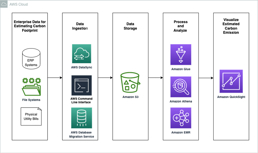

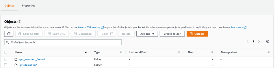
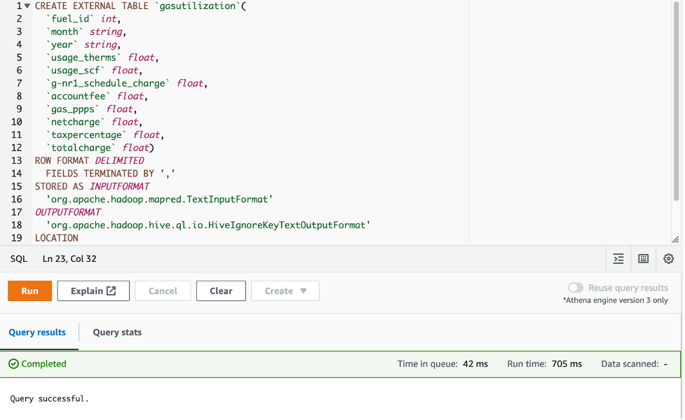
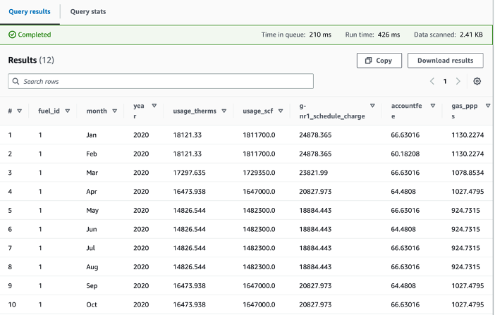
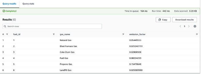
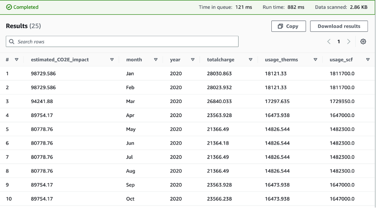
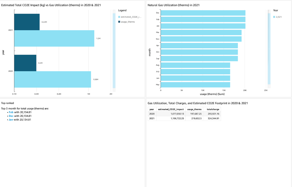
 Thomas Burns,
  Aileen Zheng is a Solutions Architect supporting US Federal Civilian Sciences customers at Amazon Web Services (AWS). She partners with customers to provide technical guidance on enterprise cloud adoption and strategy and helps with building well-architected solutions. She is also very passionate about data analytics and machine learning. In her free time, you’ll find Aileen doing pilates, taking her dog Mumu out for a hike, or hunting down another good spot for food! You’ll also see her contributing to projects to support diversity and women in technology.


 Nihar Sheth is a Senior Product Manager on the Amazon Kinesis Data Streams team at Amazon Web Services. He is passionate about developing intuitive product experiences that solve complex customer problems and enable customers to achieve their business goals.
 Pratik Patel is Sr. Technical Account Manager and streaming analytics specialist. He works with AWS customers and provides ongoing support and technical guidance to help plan and build solutions using best practices and proactively keep customers’ AWS environments operationally healthy.
 Nisha Dekhtawala is a Partner Solutions Architect and data analytics specialist. She works with global consulting partners as their trusted advisor, providing technical guidance and support in building Well-Architected innovative industry solutions.


 Mitesh Patel is a Principal Solutions Architect at AWS with specialization in data analytics and machine learning. He is passionate about helping customers building scalable, secure and cost effective cloud native solutions in AWS to drive the business growth. He lives in DC Metro area with his wife and two kids.
 Sumitha AP is a Sr. Solutions Architect at AWS. She works with customers and help them attain their business objectives by designing secure, scalable, reliable, and cost-effective solutions in the AWS Cloud. She has a focus on data and analytics and provides guidance on building analytics solutions on AWS.
 Deepti Venuturumilli is a Sr. Solutions Architect in AWS. She works with commercial segment customers and AWS partners to accelerate customers’ business outcomes by providing expertise in AWS services and modernize their workloads. She focuses on data analytics workloads and setting up modern data strategy on AWS.
 Deepthi Paruchuri is an AWS Solutions Architect based in NYC. She works closely with customers to build cloud adoption strategy and solve their business needs by designing secure, scalable, and cost-effective solutions in the AWS cloud.


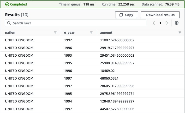
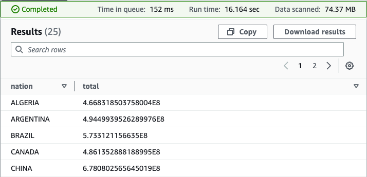
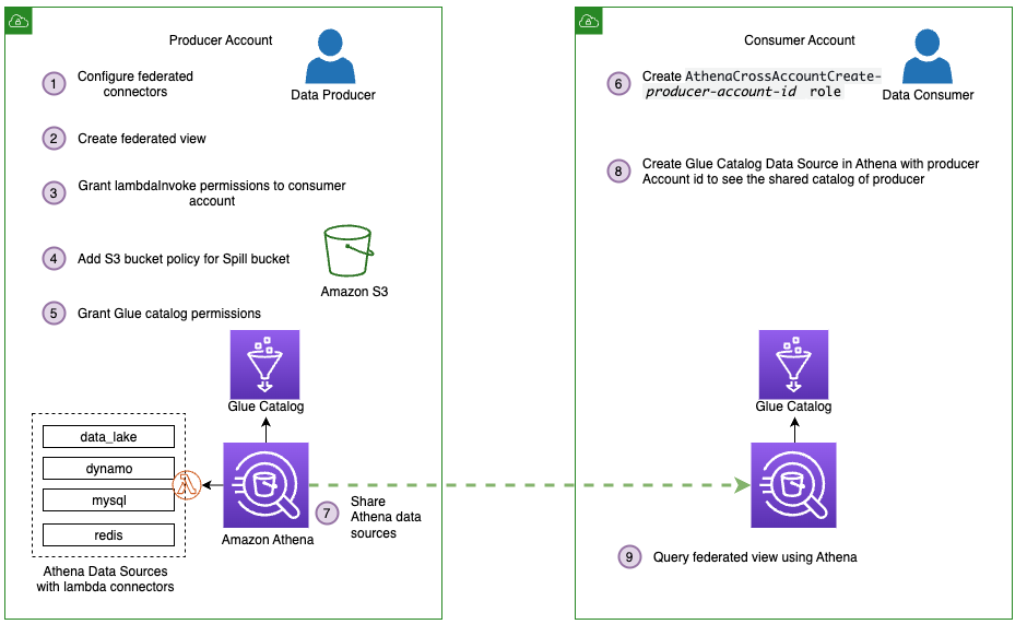
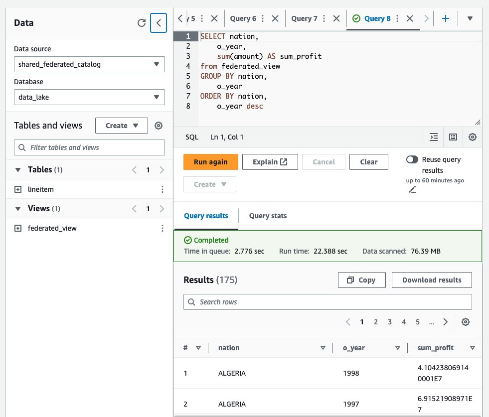

 Pathik Shah is a Sr. Big Data Architect on Amazon Athena. He joined AWS in 2015 and has been focusing in the big data analytics space since then, helping customers build scalable and robust solutions using AWS analytics services.


 Praveen Kumar is an Analytics Solution Architect at AWS with expertise in designing, building, and implementing modern data and analytics platforms using cloud-native services. His areas of interests are serverless technology, modern cloud data warehouses, streaming, and ML applications.
 Srividya Parthasarathy is a Senior Big Data Architect on the AWS Lake Formation team. She enjoys building data mesh solutions and sharing them with the community.
 Paul Villena is an Analytics Solutions Architect in AWS with expertise in building modern data and analytics solutions to drive business value. He works with customers to help them harness the power of the cloud. His areas of interests are infrastructure as code, serverless technologies, and coding in Python.
 Mostafa Safipour is a Solutions Architect at AWS based out of Sydney. He works with customers to realize business outcomes using technology and AWS. Over the past decade, he has helped many large organizations in the ANZ region build their data, digital, and enterprise workloads on AWS.


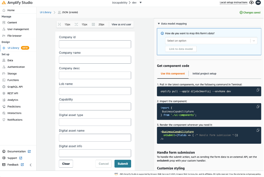

 Abdul Qadir is an AWS Solutions Architect based in New Jersey. He works with independent software vendors in the Northeast and provides customer guidance to build well-architected solutions on the AWS cloud platform.
 Sharon Li is a solutions architect at AWS, based in the Boston, MA area. She works with enterprise customers, helping them solve difficult problems and build on AWS. Outside of work, she likes to spend time with her family and explore local restaurants.


 Yash Bindlish is a Enterprise Support Manager at Amazon Web Services. He has more than 17 years of industry experience including roles in cloud architecture, systems engineering, and infrastructure. He works with Global Enterprise customers and help them build, scalable, modern and cost effective solutions on their growth journey with AWS. He loves solving complex problems with his solution-oriented approach.
 Shivani Reddy is a Technical Account Manager (TAM) at AWS with over 12 years of IT experience. She has worked in a variety of roles, including application support engineer, Linux systems engineer, and administrator. In her current role, she works with global customers to help them build sustainable software solutions. She loves the customer management aspect of her job and enjoys working with customers to solve problems and find solutions that meet their specific needs.


 Vivek Kansal works with the Amazon OpenSearch team. In his role as Principal Software Engineer, he uses his experience in the areas of security, policy engines, cloud-native solutions, and networking to help secure customer data in OpenSearch Service and OpenSearch Serverless in an evolving threat landscape.